proceedings of the fourth international workshop on

Proceedings of

the Fourth International Workshop onCooperative Distributed Vision

March 22–24, 2001

Kyoto, Japan

Sponsored by

Cooperative Distributed Vision ProjectJapan Society for the Promotion of Science

All rights reserved. Copyright c©2001 of each paper belongs to its author(s).

Copyright and Reprints Permissions: The papers in this book compromise the proceed-

ings of the workshop mentioned on the cover and this title page. The proceedings are not

intended for public distribution. Abstraction and copying are prohibited. Those who want

to have the proceedings should contact with [email protected]

Contents

1 Cooperative Behavior Acquisition by Learning and Evolution of Vision-

Motor Mapping for Mobile Robots

Minoru Asada, Eiji Uchibe, and Koh Hosoda 1

i

Cooperative Behavior Acquisition by Learning andEvolution of Vision-Motor Mapping for Mobile

Robots

Minoru Asada, Eiji Uchibe, and Koh HosodaDept. of Adaptive Machine Systems

Graduate School of Engineering

Osaka University

e-mail: [email protected]

http://www.er.ams.eng.osaka-u.ac.jp/

Abstract

This paper proposes a number of learning and evolutionary methods con-

tributed to realize cooperative behaviors among vision-based mobile robots

in a dynamically changing environment. There are three difficult problems:

partial observation, credit assignment, and synchronized learning. In order to

solve these problems, we propose the fundamental model called Local Predic-

tion Model, which can estimates the relationships between learner’s behaviors

and other agents’ ones through interactions. Based on this model, several

methods are constructed and integrated with the reinforcement learning and

evolutionary computation. All proposed methods are evaluated in the context

of RoboCup.

1 Introduction

Building a robot that learns to accomplish a task through visual information has been

acknowledged as one of the major challenges facing vision, robotics, and AI. In such an

agent, vision and action are tightly coupled and inseparable [1]. For instance, we, human

beings, cannot see anything without the eye movements, which may suggest that actions

significantly affect the vision processes and vice versa. There have been several approaches

which attempt to build an autonomous agent based on tight coupling of vision (and/or

other sensors) and actions [17, 18, 20]. They consider that vision is not an isolated process

but a component of the complicated system (physical agent) which interacts with its

environment [2, 8, 21]. This is a quite different view from the conventional CV approaches

that have not been paying attention to physical bodies. A typical example is the problem

of segmentation which has been one of the most difficult problems in computer vision

because of the historic lack of the criterion: how significant and useful the segmentation

results are. These issues would be difficult to be evaluated without any purposes. That is,

instinctively task oriented. However, the problem is not the straightforward design issue

1

2 Fourth Int. Workshop on Cooperative Distributed Vision

for the special purposes, but the approach based on physical agents capable of sensing and

acting. That is, segmentation and its organization correspond to the problem of building

the agent’s internal representation through the interactions between the agent and its

environment.

From a viewpoint of Cooperative Distributed Vision system, integration of vision, action,

and communication has been one of the central issues to realize autonomous cooperative

agents [14]. With respect to the role of communication among agents, the formulation

can be categorized into the following three patterns. Let xi and ui be a state vector and

an action vector of the robot Ri, respectively.

1. multiagent system with one central controller

Decision of all the robots are performed by one controller. In other words,

u = f(x1,x2, · · · , xn),

where uT = [uT1 uT

2 · · · uTn ]. In this case, communication among agents is realized

without any restriction. This formulation can be regarded as the one of the robot

with multiple degrees of freedom.

2. multiagent system with “explicit communication”

In this paper, “explicit communication” means that the robot can obtain the internal

states about other robots. However, each robot has its own policy function as

follows:

ui = f i(x1,x2, · · · , xn), (i = 1, · · · , n).

3. multiagent system with “implicit communication”

Because true internal states of other robots can not be observed, each robot has to

identify the internal states of other robots based on its own information.

ui = f i(x̂1, · · · , x̂i−1,xi, x̂i+1, · · · , x̂n), (i = 1, · · · , n),

where x̂ denotes the estimation of x.

In the second case, there are a number of research issues such as the realization of mu-

tual agreement among the robots, communication protocol, unreliable communication

(transmission reliability or bandwidth limits), and so on. Third is the most difficult situ-

ation. However, this includes interesting research issue [3]: How can the robots establish

non-verbal communication based on observation and action? Therefore, the aim of this

research is to develop a learning algorithm to obtain complicated behaviors under the

second or third situation. Generally, we have the following three difficult problems in

multiagent simultaneous learning:

Fourth Int. Workshop on Cooperative Distributed Vision 3

A Partial observation : Usual situated agents can only rely on an imperfect, local and

partial perception of their environment. Then, the global state of the system stays

unknown, which prevents classical reinforcement learning algorithms from finding

an optimal policy.

B Credit assignment : If the credit involves group evaluation only, one robot may accom-

plish a given task by itself and others do just actions irrelevant to the task as they

do not seem to interfere the one robot’s actions. Else, if only individual evaluation

is involved, robots may compete each other. This trade-off should be carefully dealt.

C Synchronized learning : If the multiple robots learn the behaviors simultaneously, the

learning process may be unstable, especially in the early stage of learning. If the one

robot obtains the behaviors much faster, the other could not improve its strategy

against the difficult environment.

To solve three problems, we develop several learning and evolutionary methods. All

methods are realized using no or a few explicit communication. They are listed as below:

Answer for the problem A

The problem A is called perceptual aliasing problem [7] in the context of Reinforcement

Learning (hereafter, RL). We propose the Local Prediction Model (hereafter, LPM) that

estimates the relationships between learner’s behaviors and other agents’ ones in the

environment through interactions using the method of system identification. Next, RL is

performed to obtain the optimal behavior. LPM is shown in section 2. In addition, we

accelerate the speed of learning based on the LPM. Since the expected learning time is

exponential in the size of the state space [31], it should be better to prepare the compact

state space. Based on this method, the agent gradually increase the size of the state space

according to the difficulties of the given task. This technique is explained in section 3.

Perceptual aliasing problem is also revealed when we integrate the RL and teaching

method. Because the state spaces of the learner and the teacher are different each other,

consistent instructions from the teacher are not always consistent from the viewpoint of

the learner. Therefore, we propose a method of state space construction based on the

clustering method in section 4. In this method, the learner finds taught data inconsistent

with learner’s state space, and modifies its state space so that it can successfully achieve

the goal by RL.

Answer for the problem B

One idea is to consider not only the individual evaluation functions but also the whole

ones including cooperative factors. The problem is how the agents should cope with the

multiple evaluation functions because there is usually tradeoff between individual and


team utilities. Simple implementation is a weighted summation. We propose a method

which modifies weights based on the change of the evaluation through the evolution. This

method is called adaptive fitness function, described in section 5. Another approach is

to extend the scalar evaluation function to the vector one. We formalize the multiple

reward function in section 6. This method can reconstruct the reward space so that RL

approximates the vector value function independently.

Another idea is to divide the multiple evaluation functions. That is, multiple agents take

partial charge of the multiple evaluation functions. The problem is an incompatibilities of

them. Therefore, we propose conflict resolution which can automatically allocate multiple

tasks to the multiple robots. This method is described in section 7.

Answer for the problem C

Learning schedule is proposed to make the learning process stable. At first, we select

one robot to make learn, and fix the policy of other robots. Other robots than the learning

one are stationary in the first period of behavior learning. After the learning robot finishes

learning, we select one of the other robots. We repeat this for the all robots to acquire

their purposive behaviors. This is explained in section 2.3.

Third approach is to use a co-evolutionary technique to realize synchronized learning.

The complexity of the problem can be explained twofold: co-evolution for cooperative

behaviors needs exact synchronization of mutual evolutions, and co-evolution requires

well-complicated environment setups that may gradually change from simpler to more

complicated situations. This technique is described in section 8.

All proposed methods are evaluated in the context of RoboCup [10] which is an increas-

ingly successful attempt to promote the full integration of AI and robotics research, and

many researchers around the world have been attacking a wide range of research issues.

2 LPM: Local Prediction Model

In a multiagent environment, the standard RL does not seem applicable because the envi-

ronment including the other learning agents seems to change randomly from a viewpoint

of the learning agent. Therefore, the learning agents in multiagent environments need

appropriate state representation in order for learning algorithms to converge safely.

What the learning agent can do is an acquisition of state representation taking account

of a trade-off between the number of parameters and the prediction error from the se-

quences of observation and learner’s action. In order to acquire such a model, we propose

Local Prediction Model (hereafter, LPM). About the details of LPM, one can find other

publications [6].


2.1 Acquisition of LPM from observation and action

2.1.1 State vector estimation

We utilize Canonical Variate Analysis (hereafter, CVA) [12] which is one of the subspace

state space identification methods. CVA is one of such algorithms, which uses canonical

correlation analysis to construct a state vector. Here, we give a brief explanation of CVA

method.

CVA uses a discrete time, linear, state space model as follows: Let be the input and

output generated by the unknown system

xt+1 = Axt + But,

yt = Cxt + Dut,(1)

where x ∈ <n, u ∈ <m and y ∈ <q denote state vector, action code vector, and obser-

vation vector, respectively. Further, A ∈ <n×n, B ∈ <n×m, C ∈ <q×n, and D ∈ <q×m

represent parameter matrices.

The state vector x is represented as a linear combination of the previous observation

and action sequences

xt = [In ]Mpt, (2)

where M ∈ <l(m+q)×l(m+q), and In denote the memory matrix, and the identity matrix

(n×n), respectively. Memory matrix M is calculated by CVA. Now, we follow the simple

explanation of the CVA method.

1. For {u(t), y(t)}, t = 1, · · ·N , construct new vectors

pt = [ut−1 · · · ut−l yt−1 · · · yt−l], and f t = [yt yt+1 · · · yt+l−1]. (3)

2. Compute estimated covariance matrices Σ̂pp, Σ̂pf and Σ̂ff .

3. Compute singular value decomposition

Σ̂−1/2

pp Σ̂pfΣ̂−1/2

ff = U auxSauxVTaux, (4)

where U auxUTaux = I l(m+q) and V auxV

Taux = I lq. Memory matrix M is defined as:

M := UTauxΣ̂

−1/2

pp .

4. Calculate the state vector by Eq.(2).

5. Estimate the parameter matrix applying least square method to Eq (1).

Strictly speaking, all the agents do in fact interact with each other, therefore the learning

agent should construct the local predictive model taking these interactions into account.

However, it is intractable to collect the adequate input-output sequences and estimate the

proper model because the dimension of state vector increases drastically. Therefore, the

learning (observing) agent applies the CVA method to each (observed) agent separately.


2.1.2 Determination of parameters in LPM

It is important to decide the dimension n of the state vector x and lag operator l that tells

how long the historical information is related in determining the size of the state vector

when we apply CVA to the classification of agents. Although the estimation is improved

if l is larger and larger, much more historical information is necessary. However, it is

desirable that l is as small as possible with respect to the memory size. For n, complex

behaviors of other agents can be captured by choosing the order n high enough.

In order to determine n, we apply Akaike’s Information Criterion (AIC) which is widely

used in the field of time series analysis. AIC is a method for balancing precision and

computation (the number of parameters). Let the prediction error be ε and covariance

matrix of error be

R̂ =1

N − 2l + 1

N−l+1∑

t=l+1

εtεTt .

Then AIC(n) is calculated by

AIC(n) = (N − 2l + 1) log ||R̂||+ 2λ, (5)

where λ is the number of the parameters. The optimal dimension n∗ is defined as n∗ =

arg min AIC(n). Detailed procedure is described as follows:

1. Memorize the q dimensional vector yt about the agent and m dimensional vector

ut as a motor command.

2. From l = 1 · · ·, identify the obtained data.

(a) If log ||R̂|| < a threshold, stop the procedure and determine n based on AIC(n),

(b) else, increment l until the condition (a) is satisfied or AIC(n) does not decrease.

2.2 Reinforcement learning

After obtaining LPM for each object, the agent begins to learn behaviors using RL which

is a kind of unsupervised learning, and improves its policy based on the delayed rein-

forcement without explicit state transition probabilities. The robot senses the current

state of the environment and selects an action. Based on the state and the action, the

environment makes a transition to a new state and generates a reward that is passed back

to the robot. Through these interactions, the robot learns a purposive behavior to achieve

a given goal.

Q learning [30] is a form of reinforcement learning based on stochastic dynamic program-

ming. It provides robots with the capability of learning to act optimally in a Markovian


environment. In Q learning, the action value function Q(x,u) is defined in terms of state

x and action u. Now we consider transitions from xt to xt+1 by executing u, and learn

the value Q(x,u). The action value function is updated by

Qt+1(xt,u) = Qt(xt, u) + α

[r + γ max

b∈UQt(xt+1, b)−Qt(xt,u)

], (6)

where α is a learning rate parameter and γ is a fixed discounting factor between 0 and

1. In section 2.1, appropriate dimension n of the state vector x is determined, and the

successive state is predicted. Therefore, we can regard an environment as Markovian.

2.3 Learning schedule for multiagent simultaneous learning

In a multiagent environment, there are uncertainties of state transition due to unknown

policies of other learning agent. If the multiple robots learn the behaviors simultaneously,

the learning process may be unstable, especially in the early stage of learning.

Therefore, we need a method which can stabilize the learning processes especially in

the early stage of learning. At first, the designer selects one learning agent at random

from multiple learning agents. Unselected agents do not update its own action value

function and move around based on the policy which is previously acquired. Therefore,

the selected agent is the only agent that can choose an action freely in the environment

at that time. After the selected agent has finished its learning, the designer changes the

next agent to be learned. We repeat this for robots to acquire the purposive behaviors.

2.4 Experiments

2.4.1 Task and assumptions

We have selected a simplified soccer game consisting of two mobile robots as a testbed.

RoboCup [10] has been increasingly attracting many researchers. Figure 1 (a) shows an

our mobile robot, a ball, and a goal. The environment consists of a ball, two goals, and

two robots. The sizes of the ball, the goals and the field are the same as those of the

middle-size real robot league of RoboCup Initiative. The robots have the same body

(power wheeled steering system) and the same sensor (on-board TV camera). As motor

commands, each mobile robot has two DOFs.

The output (observed) vectors are shown in Figure 1 (b). In case of the ball, the

center position, the radius, and the area of the ball image are used [6]. As a result, the

dimension of the observed vector about the ball, the goal, and the other robot are 4, 11,

and 5 respectively.


goalballother robot

(a) our mobile robot (b) image features

Figure 1: Our mobile robot and image features as observation vectors

2.4.2 Settings

At first, the shooter and the passer construct LPMs for the ball, the goal, and the other

robot in computer simulation. Next, the passer begins to learn the behaviors under the

condition that the shooter is stationary. After the passer has finished its learning, we fix

the policy of the passer. Then, the shooter starts to learn shooting behaviors. We assign

a reward value 1 when the shooter shoots a ball into the goal and the passer passes the

ball toward the shooter. Further, a negative reward value −0.3 is given to the robots

when a collision between two robots is happened. In these processes, the modular RL is

applied for shooter (passer) to learn shooting (passing) behaviors and avoiding collisions.

Next, we transfer the result of computer simulation to the real environments. In order

to construct LPMs in the real environment, the robot selects actions using the probability

based on the semi uniform undirected exploration. In other words, the robot executes

random actions with a fixed probability (20 %) and the optimal actions learned in com-

puter simulation (80 %). We performed 100 trials in real experiments. After LPMs are

updated, the robots improve the action value function again based on the obtained real

data. If LPM in the real environment increases the estimated order of the state vector,

the action value functions are initialized based on the action value functions in computer

simulation in order to accelerate the learning. Finally, we performed 50 trials to check

the result of learning in the real environment.

2.4.3 Experimental results

Table 1 shows the result of the estimated state vectors in computer simulation and real

experiments. In order to predict the successive situation, l = 1 is sufficient for the goal,

while the ball needs two steps. We suppose the reasons why the estimated orders of state


Table 1: Differences of the estimated dimension (simulation → simulation → real exper-

iments)

observer target estimated dimension (order) historical length

goal 2 → 2 → 3 1 → 1 → 1

shooter ball 4 → 4 → 4 2 → 2 → 4

passer 6 → 6 → 4 3 → 3 → 5

goal 3 → 3 → 3 2 → 2 → 2

passer ball 4 → 4 → 4 2 → 2 → 4

shooter 5 → 5 → 4 3 → 3 → 5

vectors are different between computer simulation and real experiments are :

• because of noise, the prediction error of real experiments is much larger than that

of computer simulation, and

• in order to collect the sequences of observation and action, the robots do not select

the random action but move based on the result of computer simulation. Therefore,

the experiences of passer and shooter are quite different from each other.

As a result, the historical length l of the real experiments is larger than that of the

computer simulation. On the other hand, the estimated order of state vector n for the

other robot of real experiments is smaller than that of computer simulation since the

components for higher and more complicated interactions can not be discriminated from

noise in the real environments.

Table 2 shows the comparison of performance between the simple transfer of the result

of computer simulation and the result of re-learning in real environments. We checked

what happened if we replace LPMs between the passer and the shooter. Eventually,

large prediction errors of both sides were observed. Therefore LPMs can not be replaced

between physical agents.

Table 2 shows the comparison of performance between the simple transfer of the result

of computer simulation and the result of re-learning in real environments. We checked

what happened if we replace LPMs between the passer and the shooter. Eventually,

large prediction errors of both sides were observed. Therefore LPMs can not be replaced

between physical agents.


Table 2: Performance result in real experiments

before learning after learning

success of shooting 57/100 32/50

success of passing 30/100 22/50

number of collisions 25/100 6/50

average steps 563 483

2.5 Discussion

We presents Local Prediction Model to apply RL to the environment including other

agents. Our method takes account of the trade-off among the precision of prediction,

the dimension of state vector and the length of steps to predict. Spatial quantization of

the image into objects has been easily solved by painting objects in single color different

from each other. Rather, the organization of the image features and their temporal

segmentation for the purpose of task accomplishment have been done simultaneously by

the method.

In the current LPM, we need a quantization procedure of the estimated state vectors.

Several segmentation methods such as Parti game algorithm [16] and Asada’s method

[5] might be promising. In addition, the current implementation of LPM is off-line.

Therefore, it seems difficult to apply our approach to dynamically changing environments.

It is possible to compute the state vector while we update the covariance matrices on-line.

In addition, singular value decomposition might be performed on-line by neural networks.

3 Acceleration of RL based on LPM

From a viewpoint of designing robots, there are two main issues to be considered: (1) the

design of the agent architecture by which a robot develop through interactions with its

environment to obtain the desired behaviors, and (2) the policy how to provide the agent

with tasks, situations, and environments so as to develop the robot. When the given

tasks are too difficult for the learner to accomplish them, the reward is seldom given to

the learner.

The former has revealed the importance of “having bodies” and eventually also a view

of the internal observer [23]. Asada [3] discussed how the physical agent can develop

through interactions with its environment according to the increase of the complexity of

its environment in the context of a vision-based mobile robot. In this chapter, we put


more emphasis on the second issue, that is, how to control the environmental complexity

so that the mobile robot can efficiently improve its behaviors.

Leaning from Easy Missions (LEM) paradigm was proposed [4] in which the learning

time of the exponential order in the size of the state space can be reduced to the linear

order. The basic idea of LEM paradigm can be extended to more complicated tasks, but

more fundamental issues to be considered are how to define complexity of the task and

the environment, and how to increase the complexity to develop robots. Since these issues

are too difficult to deal with as general ones, a case study on a vision-based mobile robot

is given in this section where the environmental complexity is defined in the context of

robot soccer playing and a method to control the environmental complexity is proposed

in which some periods are found and used to decide when to increase the complexity and

how much. About the details, one can find other publications [26].

3.1 An overview of the whole system

LPM outputs the state vector list in the order of the value of the estimated correlation

coefficient with estimation errors. These state vectors are used to construct the state space

for RL to be applied in multiagent environment. Here, we focus on how to accelerate the

Q-learning by appropriately increasing the environmental complexity.

One can use all the state vectors to make the robot learn, but it would take enormously

long time due to the large size of the state space. Instead of using the all vectors, one

can start with a small size of the state vector set first and increase the dimension of the

state space in the following stages. The action value function in the previous stage works

as a priori knowledge so as to accelerate the learning. In order to transfer the knowledge

smoothly, the state spaces in both the previous and current stages should be consistent

with each other. An algorithm to control the increase of the environmental complexity is

given in Figure 2.

1. Collect many sequences of data during action executions in the most complex task

environment.

2. Construct the local predictive model to the data and output the state vector lists with

estimation errors.

3. Set up the performance criterion.

4. Start with the minimum state vector set, say one or two dimensions for the lowest

complexity of the task environment.

5. Keep the complexity until the robot learns the desired behavior (reach the performance

criterion).

6. If the robot reaches the performance criterion, increase the complexity and return Step


desired behavior?

start learning with theminimal state vector set

for a while

behavior learning usingreinforcement learning

yes increase thedimension

no

performancecriterion

start

increase thecomplexity

Figure 2: A flowchart of environmental complexity control method

5. Else, increase the dimension of the state space (add a new axis) and return Step 5.

As a learning method, we use modular RL [25] based on Q learning with the state

space specified. Modular RL can coordinate multiple behaviors (in the following, shooting

behavior and avoiding one) taking account of a trade-off between the learning time and

the performance.

3.2 Experimental results

We apply the proposed method to a simplified soccer game including two agents [25]. One

is a learner to shoot a ball into a goal, and the other is a goal keeper of which speed is a

control parameter in the environment complexity.

At first, we demonstrate the experiments to control the complexity of the interactions

in case of the fixed dimension of the estimated state vector about the goal keeper. Figures

3 (a) and (b) show graphs of the performance data (success rates of shooting and collision

avoidance). The speed of the defender is increased when the robot achieves the pre-

specified success rate (80%) or no improvement can be seen. The arrows show the time

when the speed of the defender is changed (10 % speed increase of the maximum motion

speed vmax from 0 (stationary)). In spite of the number of dimensions, the best success

rate of shooting is about 80 %. However it takes much time for learning agent to acquire

the best performance when the dimension of the state space for the goal keeper increases.


0

20

40

60

80

100

0 20 40 60 80 100

perc

ent (

%)

trial (× 100)

shootcollision

0

20

40

60

80

100

0 100 200 300 400 500 600 700 800

perc

ent (

%)

trial (× 100)

shootcollision

0

20

40

60

80

100

0 50 100 150 200 250

perc

ent (

%)

trial (× 100)

shootcollision

threshold

(a) n = 1 (b) n = 4 (c) variable dimension

Figure 3: The success rate with the fixed dimension

Figure 3 (c) shows the result of the speed control for efficient learning. We set up 50%

performance criterion by which the timing of the speed increase of the defender is decided.

Compared with Figures 3 (a) and (b), we may conclude that the fewer dimensions of the

state space contribute to the reduction of the learning time but less performance and vice

versa.

Our proposed scheduling method can achieve the almost the same performance faster

than the case of learning by the maximum dimension of the state vector from the be-

ginning. We suppose that the reasons why our method can achieve the task faster are

as follows. First, the time needed to acquire an optimal behaviors mainly depends on

the size of the state space, which are determined by the dimension of the state vector

estimated by LPM. Second, since our proposed method utilizes the action value function

which is previously acquired as the initial value, it can reduce the learning time.

3.3 Discussion

We have shown the method of controlling the environmental complexity along with a

simplified soccer task. There are two main issues to be considered. First, the number

of control parameters is one in our experiments, but generally multiple, each of which

is related to each other. In such a case, since designer cannot completely understand

the relationships among them, it seems difficult to decide how to control the complexity

completely.

Then, the second issue is revealed. To cope with unknown complexity, the robot should

estimate the state vectors anytime when the task performance becomes worse. However,

this causes inconsistency in state vector sets between the current and next learning stages.

Therefore, the knowledge transfer is limited to the initial controller.


4 Integration of RL and teaching

Direct teaching seems an efficient method for a teacher to give an explicit instruction

to a learning robot so that it can achieve its goal. However, the teacher needs to have

more knowledge on the learner’s state and/or to give more frequent instructions for its

successful teaching to the robot that has less capabilities of instruction understanding and

self-learning.

We propose an active learning method by which the learner has capabilities of self-

learning and understanding the instructions by coping with cross perceptual aliasing prob-

lem. The learner asks the teacher to give an appropriate instruction when necessary to

reduce the instruction frequency. The instruction request is triggered by the decrease of

success rate or no change of action values in Q learning [30], both of which may happen

when the environment changes or the early stage of learning. Further, the learner find-

s such taught data inconsistent with learner’s state space, and modifies its state space

based on the clustering method C4.5 [19] so that it can successfully achieve the goal by

reinforcement learning. About the details, one can find other publications [15].

4.1 Active learning from cross perceptual aliasing

4.1.1 Teaching request

In order to reduce the teaching loads (to decide when and how often to give instructions),

the learner should send a teaching request to the teacher based on some criteria that can

be expected to realize the minimum instructions with the maximum learning efficiency.

Q values [30] and the success rate can be considered as such criteria because the fol-

lowing situations may correspond to the time to send a teaching request.

• If Q-values do not change for a specified period, then the learner assumes that it is

far from the rewards, and send a teaching request to lead itself somewhere near the

rewards.

• If the success rate decreases, then the learner assumes that the environment changes,

and send a teaching request to show a sequence of actions leading to the goal.

The whole procedure to send a teaching request is given as follows (see Figure 4 (a)).

1. Prepare the learner’s state space.

2. Learner: Apply reinforcement learning (one step Q-learning). Action selection is

done by the best policy, instructed action if any, or random.


action selection

Q mapmonitor

(Q values)

(success rate)

instructed datastorage

(s1, a1)(s2, a2)

:(sn, an)

request instructedactions

action state (s)

learner

teacher

environment

Axis of X

action a1

action a2

action a2

action a1

State Space of Teacher

State Space of Teacher

State Space of Learner

State Space of Learner

(a) integration of learning and teaching (b) aliasing between teacher and learner

Figure 4: An overview of the whole system

3. learner: If sumQ(t− T )− sumQ(t) < Crt, where t, T , and Crt denote the current

time step, the pre-specified time interval, and a constant for decision making, then

send a teaching request and goto 4. Else, goto 2.

4. (a) teacher Instruct the learner a sequence of actions to the goal from the (t−T )-th

step or from the beginning when just after the start of the trial.

(b) learner Execute the instructed actions and store the sequence of pairs { (s1, a1),

(s2, a2), · · ·, (sn, an) }. If teaching ends, then goto 2.

4.1.2 Learning from cross perceptual aliasing

As described above, the learner may not understand the instructed action by the teacher

due to cross perceptual aliasing. Since the internal representation of the world can differ

between the learner and the teacher, the instructions consistent with the teacher’s view

might be inconsistent with the learner’s view. Figure 4 (b) shows a typical example for

such a situation, where the instructed actions a1 and a2 are the most suitable ones in

states s1 and s2, respectively, but those states are not discriminated in the learner’s state

space, therefore, these actions can be regarded as inconsistent ones.

To cope with this problem, the leaner should modify its state space so that it can

represent the teacher’s state space. Then, a clustering method C4.5 [19] is applied to a

set of inconsistent actions with continuous sensory data and related information such as


historical ones near the inconsistent data. As a result of this clustering, new states are

added into the learner’s state space as shown at the bottom of Figure 4 (b).

The following procedures are included into the step 4(b) of the teaching described in

section 4.1.1.

1. The learner stores a sequence of triplet (s, a, X), where (s, a) is an instruction and

X = (x1, x2, .., xl) are attribute vector related to the instruction (s, a) such as other

sensory data or their historical ones.

2. After one teaching (a sequence of instructions): check the variance of instructions

including the past ones. If different actions for the same state were instructed, then

goto next (3). Else, skip the following and proceed the learning.

3. Check the success rate after executing the instructed actions with the current state

space. If the success rate is unsatisfactory, then goto 4. Else, skip the following and

proceed the learning.

4. Apply C4.5 to a data set (s, a, X) in terms of class a with attribute X. Clustered

regions are added to the state space as new states, and the instructed action a can

be unique in the new state space.

4.2 Task and assumptions

The task is to position itself just in front of the ball and the goal. The initial positions

are set in such a way that the robot is between the ball and the goal and orients at the

goal side.

A teacher has a global view by setting a TV camera above the field which captures the

image of the ball, the goal, and the learner together. This sensor space constructs the

teacher’s state space as it is, and the teacher sends the instructions to the leaner based

on the teacher’s current state regardless of the learner’s internal representation of the

environment.

The instruction data consist of the instructed action and related information X such as

the current sensory data and their historical ones in terms of physical clock time (30 [ms]).

Here, X includes the observed values of the centroid, the width (the radius), and the area

of the goal (ball) and the number of clocks after the robot encountered the current state.


In this task, perceptual aliasing within the learner is inherently included, that is, easily

losing the sight of the ball and/or the goal. Therefore, learning time is much longer than


Goal state ( Right lost) Ball state ( Small , Center )

new state 1

x_ball > 12 x_ball < 12

new state 2

Goal state ( Right lost ) Ball state ( Right lost )

new state 2 new state 1 new state 3

# of clock >25 # of clock < 25 image before 1step

(a) success rates with/ (b) example 1 (c) example 2

without teaching

Figure 5: Experimental results in positioning task

Figure 6: A sequence of the real experiment

the shooting task, and one block consists of 10000 trials. To avoid a trivial solution, we

limit the action set without backward motions, that is, the robot can take one of five

actions.

Figure 5 (b) and (c) shows new states in two cases. First one is the case that the state

of ball center is split into two states in order to play back the instructed actions more

precisely. The second is more complicated one including historical information in which

both-ball-and-goal-lost state is split into three new states: 1) still lost for longer than 25

clocks, 2) within 25 clocks, ball-lost-left and goal-large-right, and then lost, 3) within 25

clocks, ball-large-left and goal-lost-right, and then lost.

Figure 5 (a) shows the learning results with/without teaching request. Teaching seems

effective especially at the early stage of the learning. The learning without teaching could

not achieve any goals due to its perceptual aliasing. The arrow in the later stage indicates

the time step when the robot regarded the shift of initial position as the change of the


environment. The learned behavior seemed much robust than the instructed actions (see

Figure 6 for the real experiment).

5 Adaptive Fitness Function

In section 3, we discuss the environmental complexity. In this experiment, we found

that the robot did not obtain the good behavior if we set up the severe situation at the

beginning of learning.

In applying learning and/or evolutionary approaches to the robot, the evaluation func-

tion should be given in advance. There are two important issues when we attempt to

design the fitness function. First one is that the multiple fitness measures should be con-

sidered in order to evaluate the resultant performance. One simple realization is to create

the new scalar function based on the weighted summation of multiple fitness measures. In

this section, we propose Adaptive Fitness Function to modify the weights appropriately.

In order to obtain the policy, we select a Genetic Programming (hereafter GP) method

[11]. About the details, one can find other publications [29].

5.1 Adaptive fitness function

Suppose that n standardized fitness measures fi (i = 1, · · ·n, 0 ≤ fi ≤ 1) are given to

the robot. That is, the smaller is better. Then, we introduce a priority function pr, and

define the priority of fi as pr(fi) = i. Combined fitness function is computed by

fc =n∑

i=1

wifi, (7)

where wi denotes the weight for i-th evaluation. The robot updates wi through the

interaction with the environment.

We focus on the change of each fi and correlation matrix. Let the fitness measure of

the individual j at the generation t be fi(j, t), and we consider the change of the fitness

measures by

∆fi(t) =1

N

N∑

j=1

{fi(j, t)− fi(j, t− 1)} , (8)

where N is the number of population. In case of ∆fi > 0, i-th fitness measure is not

improved under the current fitness function. Therefore, the influence of the corresponding

weight wi should be changed. However, other fitness measures fj (j = i + 1, · · ·n) should

be also considered since they would be related to each other.


Let Ci be the set of fitness measures which is related to the i-th measure,

Ci = {j | |rij| > ε, j = i + 1, · · · , n}, (9)

where ε is a threshold between 0 and 1, and rij is a correlation between fi and fj. In

case of Ci = φ, wi can be modified independently because i-th fitness measure does not

correlate with other measures. Therefore, wi is increased so that the i-th fitness measure

would be emphasized.

In case of Ci 6= φ, wj∗ is updated, where j∗ is prior to other evaluation measures in Ci,

that is,

j∗ = arg maxj∈C i

pr(fi).

The reason why wi is not changed explicitly is that the weight of the upper fitness measure

would continue to be emphasized even if the corresponding fitness measure is saturated.

As a result, the lower fitness measure related to the upper one is emphasized directly.

The update value ∆wj∗(t) is computed by

∆wj∗(t) =

1 (rij∗ > ε)

−1 (rij∗ < −ε). (10)

It is possible for the weight corresponding to improved measures to change for the worse.

However, it would be rather unimportant measures because of the given priority.

5.2 Task, assumptions, and GP implementation

We have selected a simplified soccer game consisting of two mobile robots as a testbed.

Detailed setting is described in section 2.4.1. The task for the learner is to shoot a ball into

the opponent goal without collisions with an opponent. At the beginning, the behavior

is obtained in computer simulation, and we transfer the result of simulation to the real

robot.

Each individual has two GP trees, which control the left and right wheels, respectively.

GP learns to obtain mapping function from the image features to the motor command.

We select the terminals as the center position in the image plane. For example, in a case

of the ball, the current center position and the previous one are considered. As a result,

the number of the terminals is 4(objects) × 4(features) = 16. As a function set, we

prepare four operators such as +, −, × and /.


At first, we perform a simulation using a stationary opponent. This experiment can be

regarded as an easy situation. We compare the proposed method with the fixed weight


0

5

10

15

20

25

0 50 100 150 200

num

ber

of a

chie

ved

goal

s

number of generation

proposed method (average)proposed method (best result)

fixed weight

0

5

10

15

20

25

0 20 40 60 80 100

num

ber

of a

chie

ved

goal

s

number of generation

proposed method (average)fixed weight

(a) with the stationary opponent (b) with the moving opponent

Figure 7: Average of the number of achieved goals in the first experiment

method. Figure 7 (a) shows the result when the opponent is stationary. In a case of the

fixed weight method, the performance is not improved after the 50th generations. On the

other hand, the performance based on the proposed method is improved gradually.

Next, we show a simulation results using an active opponent. This experiment can be

regarded as a more difficult situation. As an initial population for this experiment, we

used the best population which was obtained based on the proposed method described

above. Figure 7 (b) shows a histories of fopp. In this experiment, although the opponent

just chases the ball, the speed can be controlled by the human designer. Its speed was

gradually increased at the 40th and 80th generations, respectively.

According to the increase of the speed of the opponent, the obtained scores fopp was

slightly decreased in a case of the fixed weight method. On the other hand, the robot

using the proposed method kept the performance same in spite of the increase of the

speed.

We transfer the obtained policy to the real robot. Figure 8 shows a preliminary result

of the experiments, that is, one sequence of images where the robot accomplished the

shooting behavior. This robot participated in the competition of RoboCup 99 which was

held in Stockholm.

6 Multiple Reward Criterion

In section 5, we presented one approach to cope with multiple evaluation functions. In

this section, we show alternative called Vectorized Value Function. A discounted matrix

is introduced to the value function. In this case, it is important to design it. About the


Figure 8: Typical shooting behavior in the real environment

details, one can find other publications [24].

The proposed architecture is implemented using actor-critic [22]. The critic is a vector-

ized state value function. After each action selection, the critic evaluates the new state

to determine whether it has become better or worse than expected.

6.1 Vectorized reinforcement learning

Considering the above mentioned issue, we extend scalar value function to a vectorized

value function. The discounted sum of the vectorized value function can be expressed by

vt(xt) =∞∑

n=0

Γ nrt+n, (11)

where Γ is N ×N matrix. We call Γ discounted matrix.

It is important to design Γ . We utilize the principal angles between two subspaces in

order to determine Γ . A merit of this method is reduction of the size of the reward space

if there is a bias when the rewards are given to the robot. Taking into account the reward

space, we can modify the state space appropriately while the state space is constructed

based on only the sequences of observation and action in LPM.

In order to calculate the principal angles, we have to compute the following singular

value decomposition

Σ̂−1/2

rr Σ̂rx = U 2S2VT2 , (12)


where U 2UT2 = IN and V 2V

T2 = In. This computation is the almost same as Eq.(4).

We set Γ as

Γ = S2 = diag [cos θ1, cos θ2, · · · , cos θN ] , (13)

where θ (θ1 ≤ θ2 ≤ · · · ≤ θN ≤ π/2) denotes the principal angle between two subspaces

(S(R) and S(X)). Furthermore, we modify the new reward and state spaces as follows:

r′ = UT2 Σ̂

−1/2

rr r and, x′ = V T2 x. (14)

The robot learns its behavior based on the new reward r′ and the new state vector x′.

Because the eigenvalues of Γ in Eq.(13) are less than one, the value expressed by Eq.(11)

converges.

6.2 Behavior learning

In order to acquire the policy, we utilize the actor-critic methods [22] which are TD ones

that have a separate memory structure explicitly. Let qt(x′,u) be a vector at time t for

the modifiable policy. The TD error can be used to evaluate the action u taken in the

state x′. Eventually, the learning algorithm is shown as follows.

1. Calculate the current state x′t by Eq.(2) and Eq.(14).

2. Execute an action based on the current policy. As a result, the environment makes a

state transition to the next state x′t+1 and generates the reward rt.

3. Calculate the TD error by

δt = r′t + Γvt(x′t+1)− vt(x

′t). (15)

and update the eligibility [22].

4. Update the value function and the policy function. For all x′t ∈ X ′ and ut ∈ U ,

vt+1(x′t) = vt(x

′t) + αδtet(x

′t), , and qt+1(x

′t,ut) = qt(x

′t,ut) + βδt, (16)

where α and β (0 < α, β < 1) are learning rate.

5. Return to 2.

The learning robot has to select several actions to explore the unknown situations.

Then, we use ε-greedy strategy [22], meaning that most of time the robot chooses an

optimal action, but with probability ε it instead selects an action at random. An optimal

action is determined as follows: Initialize rank(u) = 0 for all u ∈ U . For i = 1, · · ·N ,

1. Calculate the optimal action corresponding to each qi (qT = [q1, · · · , qN ]),

u∗i = arg maxu∈U

qi(x′,u). (17)


2. Increment rank(u∗i ) = rank(u∗i ) + 1.

3. Execute the optimal action,

u∗ = arg maxu∈U

rank(u). (18)

After all, since the all actions are ordered with respect to the Pareto optimality, the

learning robot can select the action which satisfy the optimal action as possible.


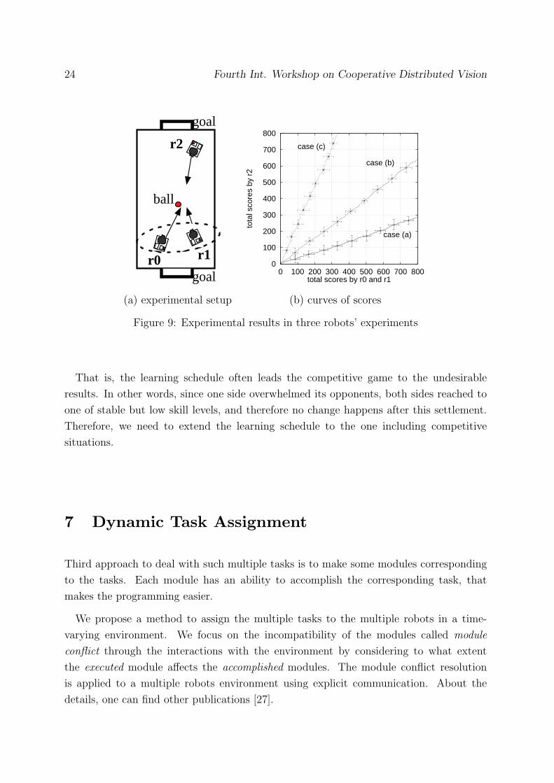
We perform three-robots’ experiments. This experiment involves both cooperative and

competitive tasks. r0 and r1 are teammates. We prepare six dimensional reward vector

is

r =

rc

rl

rm

rs

rp

rk

· · · -1 (collisions),

· · · -1 (losing scores),

· · · -1 (pass the ball to the opponent),

· · · 1 (earned scores),

· · · 1 (pass the ball to the teammate),

· · · 1 (kicking the ball).

The other parameters are set to λ = 0.4, α = 0.25 and β = 0.25, respectively.

We prepare the learning schedule to make learning stable in the early stage. We set up

the following three learning schedules,

• case (a) : r0 → r1 → r2

• case (b) : r0 → r2 → r1 → r2

• case (c) : r2 → r0 → r1

Each interval between change of learning robots is set to 2.5×104 trials. After each robot

learned the behaviors (all the robot was selected at once), we recorded the total scores in

each game.

6.4 Simplified soccer game among three robots

Figure 9 illustrates the histories of the game. As we can see from Figure 9, the result

depends on the order to learn. Although this game is two-to-one competition, r2 won

the game if we selected r2 as the first robot to learn (case (C)). Otherwise, a team of r0

and r1 defeated r2. This scheduling is a kind of teaching, help the agents to search the

feasible solutions from a viewpoint of the designer. However, the demerits of this method

is also revealed when we apply it to the competitive tasks.


r1

r2

r0

ball

goal

goal

0

100

200

300

400

500

600

700

800

0 100 200 300 400 500 600 700 800

tota

l sco

res

by r

2

total scores by r0 and r1

case (a)

case (b)

case (c)

(a) experimental setup (b) curves of scores

Figure 9: Experimental results in three robots’ experiments

That is, the learning schedule often leads the competitive game to the undesirable

results. In other words, since one side overwhelmed its opponents, both sides reached to

one of stable but low skill levels, and therefore no change happens after this settlement.

Therefore, we need to extend the learning schedule to the one including competitive

situations.

7 Dynamic Task Assignment

Third approach to deal with such multiple tasks is to make some modules corresponding

to the tasks. Each module has an ability to accomplish the corresponding task, that

makes the programming easier.

We propose a method to assign the multiple tasks to the multiple robots in a time-

varying environment. We focus on the incompatibility of the modules called module

conflict through the interactions with the environment by considering to what extent

the executed module affects the accomplished modules. The module conflict resolution

is applied to a multiple robots environment using explicit communication. About the

details, one can find other publications [27].


7.1 Module conflict resolution

For reader’s understanding, we introduce some important terms. A multitask is a com-

position of multiple tasks, where a task means transfer from the initial state to the desired

state by robot. A module consists of a policy (controller) and an evaluation function

which indicates to what extent the current task is accomplished.

Each module mk ∈M has two functions. One is a policy fk(x) which maps from a state

x to an action ok, and the other is an evaluation function vk(x). The module outputs

ok based on fk(x) in order to minimize the evaluation function vk(x). In addition, we

standardize vk(x) by

ak =

0 (vk,inf < vk(x))vk(x)− vk,inf

vk,sup − vk,inf

(vk,sup < vk(x) ≤ vk,inf)

1 (0 ≤ vk(x) < vk,sup)

, (19)

where vk,inf and vk,sup are thresholds. Hereafter, we call ak task accomplishment. Using

the task accomplishment, the subset of modules Ma is defined by Ma = {mi|ak = 1}. A

module m ∈Ma is no longer executed because it has been already accomplished.

Then, we define a new measure ei called task execution by

ei(t) = ρet(t− 1) +

(1− ρ) if mi is a selected module,

(1− ρ)ai(t) otherwise,(20)

where ρ is a forgetting factor between 0 and 1. A case of ei = 1 and ai 6= 0 means that the

robot can not minimize the evaluation function although the robot attempt to accomplish

the i-th task.

Although it is desirable for a robot to accomplish given multiple tasks, there would

be some modules incompatible to each other according to the situation. Therefore, it is

important for a robot to resolve such conflicts between the modules automatically. In

order to detect the conflict between the modules mi and mj, a correlation of ei and aj

is utilized. ∆r(ei, aj) is an index to measure how task execution of mi influences task

accomplishment of mj. The modules that are in conflict with the module mj ∈ Ma is

determined by

Mc = {mi|∆r(ei, aj) < 0, mj ∈Ma}.

In case of ∆r(ei, aj) ≥ 0, the robot can cope with both the execution of the module mi

and the accomplishment of the module mj. On the other hand, in case of ∆r(ei, aj) < 0,

the execution of the module mi prevents the accomplishment of the module mj.


The rest of the modules is determined as Mca = M−Ma −Mc. At the beginning,

Mca = M, Ma = φ, and Mc = φ. The robot selects the module by

ms = arg maxm′∈Mca

U(m′), (21)

where U is a priority which is given in advance. Ma, Mc and Mca are updated according

to the changes of the environment in order to accomplish the tasks as many as possible.

The robot follow the procedures every time step:

1. For the all modules, task accomplishment and task execution are computed using

equations (19) and (20).

2. Calculate subsets Ma, Mc, and Mca.

3. Select a module ms from Mca using equation (21).

4. Execute an action os based on the policy of the module ms.

7.2 Extension to a multiagent environment

We extend our method to a multiagent system by adding multiple robots that take charge

of Mc. We assume that (1) each robot has the same set of modules M and (2) each robot

can get the information about task accomplishment and task execution. This can be

implemented by a blackboard system. Each robot has its own parameters such as task

accomplishment, task execution, and module subsets (Ma, Mc, and Mca). Hereafter, “k”

denotes the parameter of the k-th robot kR. In order to measure how much the robot kR

works, the load kLj(t) is calculated by

kLj(t) =n∑

i=j

kaiU(mi), (22)

where U(mi) is the priority of module mi.

For the current module mj determined by Eq. (21), the robot kR judges whether mj

should be executed or not. A procedure is described as follows:

1. Check task accomplishment of mj. Go to step 4 if no robot has already accomplished

the task.

2. Check the remaining power of kR. If kL(t) < Lmax, go to step 4 (Lmax is a threshold).

3. Entrust the module mj to the other robot. Subtract mj from kMca, and add mj tokMe, where kMe denotes the subset of the modules that are accepted by other robots.

Then, return to step 1.

4. Check the module conflict. Go to step 5 if the modules mj and mi are compatible

each other. Otherwise, add mj to kMc. Then, go to step 1.


(a) Start (b) (c) (d)

(e) r1:450 (f) r0:400 (g) r1:600 (h) r0:500

(i) r1:800 (j) r0:t=600 (k) (l)

Figure 10: The result of real space experiment (robot ID:time)

5. Execute mj. If the robot Rk accomplished the module mj, transfer mj from kMc tokMa. Then, go to step 1. Otherwise, execute mj.


In this experiment, our mobile robot has an omnidirectional vision system to capture

the visual information whole around the robot. The omni-directional vision has a good

feature of higher resolution in direction from the robot to the object although the distance

resolution is poor.

We prepare four modules such as push the ball, attack, defense, and save the

goal. The policies of these modules are designed by a simple feedback controller. It is

possible to acquire them based on the our reinforcement learning algorithms described in

section 2 and 6.



Figure 10 shows an example sequence of the robots’ behaviors. For the sake of con-

venience, the robot colored in black (white) is called r0 (r1). In Figure 10 (a), r0 is the

robot in the right side. From these figures,

(a)∼(c) : Both robots moved to the own goal because the module m4 (stay at the own

goal) is the most important.

(d) : Since r0 accomplished the module m4, r1 neglected m4 and checked the task ac-

complishment of ai (i = 1, 2, 3).

(e)∼(f) : r0 stayed in front of the own goal while r1 attempted to clear the ball.

(g) : They swapped their roles.

(h), (i) : r0 attempted to push the ball by m1. In this case, m2 was also accomplished

by r0. On the other hand, r1 went to the own goal. However r1 failed to accomplish

m1 due to its poor policy.

(j)∼(l) : r0 moved to the own goal again because r1 could not reach the own goal. As a

result, r1 attempted to clear the ball again since r1 was not needed to stay at the

own goal any more.

7.5 Discussion

We have proposed a method to resolve the conflict between the given modules to handle

the multiple tasks in a multiagent environment. We have already checked the simulation

results in case of three robots.

As future work, we are developing the method to change the priority function U using

the value of evaluation function because the total performance depends on it in the current

system.

8 Co-evolution

We discuss how multiple robots can emerge cooperative and competitive behaviors through

co-evolutionary processes in this section. A genetic programming method is applied to

individual population corresponding to each robot so as to obtain cooperative and com-

petitive behaviors.

The complexity of the problem can be explained twofold: co-evolution for cooperative

behaviors needs exact synchronization of mutual evolutions, and three robot co-evolution

requires well-complicated environment setups that may gradually change from simpler to

more complicated situations. As an example task, several simplified soccer games are

selected to show the validity of the proposed methods. About the details, one can find

other publications [28].


8.1 Co-evolution in cooperative tasks

Co-evolution is one of potential solutions for the problem C described in section 1 by

seeking for better strategies in a wide range of searching area in parallel. Emerging

patterns by co-evolution can be categorized into three.

1. Cycles of switching fixed strategies : This pattern can be often observed in a

case of a prey and predator which often shift their strategies drastically to escape from

or to catch the opponent. The same strategies iterate many times and no improvements

on both sides seem to happen.

2. Trap to local maxima : This corresponds to the second problem stated above.

Since one side overwhelmed its opponents, both sides reached to one of stable but low

skill levels, and therefore no change happens after this settlement.

3. Mutual skill development : In certain conditions, every one can improve its strategy

against ever-changing environments owing to improved strategies by other agents. This

is real co-evolution by which all agents evolve effectively.

As a typical co-evolution example, a competitive task such as prey and predator has

been often argued [9] where heterogeneous agents often change their strategies to cope with

the current opponent. That is, the first pattern was observed. In a case of homogeneous

agents, Luke et al. [13] co-evolved teams consisting of eleven soccer players among which

cooperative behavior could be observed. However, co-evolving cooperative agents has

not been addressed as a design issue on fitness function for individual players since they

applied co-evolving technique to teams.

We believe that between one-to-one individual competition and team competition, there

could be other kinds of multiagent behaviors by co-evolutions than competition. Here,

we challenge to evaluate how the task complexity and fitness function affect co-evolution

processes in a case of multiagent simultaneous learning for not only competitive but also

cooperative tasks through a series of systematic experiments. First, we show the experi-

ments for a cooperative task, that is, shooting supported by passing between two robots

where unexpected cooperative behavior regarded as the second pattern was emerged.

Next, we introduce a stationary obstacle in front of the goal area into the first experimen-

tal set up, where the complexity is higher and an expected behavior was observed after

longer generation changes than the previous one. Finally, we exchange an active learning

opponent with the stationary obstacle to evaluate how both cooperative and competitive

behaviors are emerged.



The task is almost same as the one described in section 6.3. It is essential to design

the well-defined function and terminal sets for appropriate evolution processes. This can

be regarded as the same problem to construct the well-defined state space. As sets of

functions, we prepare a simple conditional branching function “IF a is b” that executes

its first branch if the condition “a is b” is true, otherwise executes its second branch,

where a is a kind of image features, and b is its category [28].

Terminals in our task are actions that have effects on the environment. A terminal set

consists of the following four behaviors based on the visual information: shoot, pass,

avoid, and search. These primitive behaviors have been obtained by the learning algo-

rithms described in section 2 in the real environment.

Another issue to apply an evolutionary algorithm is the design of fitness function which

leads robots to appropriate behaviors. We first consider the two parameters to evaluate

team behaviors: total number of obtained goals lost goals to which the robot belongs.

Then, we introduce the two individual evaluations to encourage robots to kick the ball

while minimizing the number of collisions. In addition, the toal number of steps is involved

to make robots achieve the goal earlier.


At first, we demonstrate the experiments to acquire cooperative behaviors between two

robots. Both robots belong to the same team, and they obtain the score if they succeed

in shooting a ball into the goal. The number of function sets is 28 (= 7 (ball) +2×7 (two

goals) +7 (teammate)). We call the robot expected to be a passer r0 while the robot

expected to be a shooter r1.

In computer simulation, r0 does not kick the ball by itself but shakes its body by

repeating the behaviors search and avoid. On the other hand, r1 approaches the ball

and passes the ball to r0. After r0 receives the ball, it executes a shoot behavior.

However, r1 approaches the ball faster than r0. As a result, r1 shoots the ball into

the goal while r0 avoids collisions with r0. We checked the case of the varying fitness

functions, and found that the resultant behaviors were similar to the behavior by the

fixed case. In this task, the best r0 does not kick the ball toward r1 at the end of the

generations.

We suppose that the reasons why they acquire such behaviors are as follows:

• In order for r0 to survive by passing the ball to r1, r1 has to shoot the ball which is

passed back from r0. This means that the development of both robots needs to be


Figure 11: Two robots succeed in shooting a ball into the goal

exactly synchronized. It seems very difficult for such a synchronization to be found.

• r1 may shoot the ball by itself whichever r0 kicks the ball or not. In other words,

r1 does not need the help by r0.

In this task, r0 and r1 do not have even complexities of the tasks. As a result, the

behavior of r1 dominates this task while r0 cannot not improve its own behavior.

We transfer the result of computer simulation to the real robots. Figure 11 shows an

example of obtained behaviors using two robots in the real environment. In this task, one

of the robots executed shoot behavior while the other stopped. Therefore, stopped robot

could not improve its own behavior.

Next, we add one robot called r2 as a statonary obstacle to the environment. The

number of function sets is 35 (= 7 (ball) +2 × 7 (two goals) +2 × 7 (teammate and

opponent)).

Although both learning robots are placed in the same way as in the previous exper-

iments, the acquired cooperative behaviors are quite different. We found the following

three patterns in a case of the fixed fitness function:

1. First pattern (ball rolling and accidental goal)

Because r0 is placed near the ball, r0 pushes the ball more frequently than r1.

Most of individuals of r0 kick the ball towards r1 owing to the initial placement.

However, some individuals push the ball towards r2 in the neighborhood of r0.

Consequently, the ball rolls towards the goal by accident.


Figure 12: Two robots succeed in shooting a ball into the goal against the defender

2. Second pattern (goal after dribbling along the wall)

Although both r0 and r1 kick the ball until generation 4, r0 begins to pass the ball

towards r1. However, r1 can not shoot the ball from r0 directly because r0 cannot

pass the ball to r1 precisely. Therefore, r1 kicks the ball to the wall and continues

to kick the ball to the opponent’s goal along the wall until generation 15. After

that, the rank of this pattern dropped down.

3. Third pattern (mutual skill development)

After a number of generations, both robots improve their own behaviors and acquire

cooperative behaviors at the end of generations, where r0 kicks the ball to the front

of r1, then r1 shoots the ball into the opponent’s goal shown. As a result, both

robots improve the cooperative behaviors synchronously. This is a kind of the

mutual development.

The individual of the third pattern obtained the high evaluation because it takes much

shorter time to shoot the ball than the first and second patterns.

We transfer the result of computer simulation to the real robots. Figure 12 shows an

example of obtained behaviors using two robots in the real environment.


9 Conclusion

In this paper, we propose a number of learning and evolution methods to realize cooper-

ative behaviors in a dynamically changing environment. Because our methods assume no

or a few communication among agents, it is important to construct the internal model of

other agents. In order to construct the model, we propose LPM. Furthermore, some learn-

ing and evolutionary methods are developed to realize the cooperative and competitive

behaviors based on LPM. All proposed methods are evaluated in the context of RoboCup.

Acknowledgement

We thank many people for valuable guidance and implementation of the algorithms. E-

specially, we wish to our gratitude to Yasutake Takahashi, Masateru Yanase, Chizuko

Mishima, Tatsunori Kato, and Masakazu Yanase.

References

[1] Y. Aloimonos. Introduction: Active Vision Revisited. In Y. Aloimonos, editor, Active

Perception, chapter 0, pages 1–18. Lawrence Erlbaum Associate, Publishers, 1993.

[2] Y. Aloimonos. Reply: What I have learned. CVGIP: Image Understanding, 60:1:74–

85, 1994.

[3] M. Asada. An Agent and an Environment: A View of “Having Bodies” – A Case

Study on Behavior Learning for Vision-Based Mobile Robot –. In Proc. of 1996 IROS

Workshop on Towards Real Autonomy, pages 19–24, 1996.

[4] M. Asada et al. Purposive Behavior Acquisition for a Real Robot by Vision-Based

Reinforcement Learning. Machine Learning, 23:279–303, 1996.

[5] M. Asada, S. Noda, and K. Hosoda. Action-Based Sensor Space Categorization for

Robot Learning. In Proc. of the IEEE/RSJ International Conference on Intelligent

Robots and Systems, 1996.

[6] M. Asada, E. Uchibe, and K. Hosoda. Cooperative behavior acquisition for mobile

robots in dynamically changing real worlds via vision-based reinforcement learning

and development. Artificial Intelligence, 110:275–292, 1999.


[7] L. Chrisman. Reinforcement Learning with Perceptual Aliasing: The Predictive

Distinctions Approach. In Proc. of the Tenth National Conference on Artificial In-

telligence, pages 183–188, San Jose, CA, 1992. AAAI Press.

[8] S. Edelman. Reply: Representation without Reconstruction. CVGIP: Image Under-

standing, 60:1:92–94, 1994.

[9] D. Floreano and S. Nolfi. Adaptive Behavior in Competeing Co-Evolving Species. In

Proc. of the Fourth European Conference on Artificial Life, pages 378–387, 1997.

[10] H. Kitano, ed. RoboCup-97 : Robot Soccer World Cup I. Springer Verlag, 1997.

[11] J. R. Koza. Genetic Programming I : On the Programming of Computers by Means

of Natural Selection. MIT Press, 1992.

[12] W. E. Larimore. Canonical Variate Analysis in Identification, Filtering, and Adaptive

Control. In Proc. 29th IEEE Conference on Decision and Control, pages 596–604,

Honolulu, Hawaii, December 1990.

[13] S. Luke, C. Hohn, J. Farris, G. Jackson, and J. Hendler. Co-Evolving Soccer Softbot

Team Coordination with Genetic Programming. In Proc. of the First RoboCup-97

Workshop at IJCAI’97, pages 115–118, 1997.

[14] T. Matsuyama. Cooperative Distributed Vision – Dynamic Integration of Visual Per-

ception, Action, and Communication –. In Proc. of Image Understanding Workshop,

Monterey CA, 11 1998.

[15] C. Mishima and M. Asada. Active Learning from Cross Perceptual Aliasing Caused

by Direct Teaching. In Proc. of the IEEE/RSJ International Conference on Intelli-

gent Robots and Systems, pages 1420–1425, 1999.

[16] A. W. Moore and C. G. Atkeson. The Parti-game Algorithm for Variable Resolu-

tion Reinforcement Learning in Multidimensional State-spaces. Machine Learning,

21:199–233, 1995.

[17] T. Nakamura and M. Asada. Motion Sketch: Acquisition of Visual Motion Guided

Behaviors. In Fourteenth International Joint Conference on Artificial Intelligence,

pages 126–132. Morgan Kaufmann, 1995.

[18] T. Nakamura and M. Asada. Stereo Sketch: Stereo Vision-Based Target Reaching

Behavior Acquisition with Occlusion Detection and Avoidance. In Proc. of the IEEE

International Conference on Robotics and Automation, pages 1314–1319, 1996.


[19] J. R. Quinlan. C4.5: Programs for Machine Learning. Morgan Kaufman, San Mateo,

CA, 1993.

[20] G. Sandini. Vision during action. In Y. Aloimonos, editor, Active Perception, chap-

ter 4, pages 151–190. Lawrence Erlbaum Associate, Publishers, 1993.

[21] G. Sandini and E. Grosso. Reply: Why Purposive Vision. CVGIP: Image Under-

standing, 60:1:109–112, 1994.

[22] R. S. Sutton and A. G. Barto. Reinforcement Learning. MIT Press/Bradford Books,

March 1998.

[23] J. Tani. Cognition of Robots from Dynamical Systems Perspective. In Proc. of 1996

IROS Workshop on Towards Real Autonomy, pages 51–59, 1996.

[24] E. Uchibe and M. Asada. Multiple reward criterion for cooperative behavior acqui-

sition in a multiagent environment. In Proc. of IEEE International Conference on

Systems, Man, and Cybernetics, 1999.

[25] E. Uchibe, M. Asada, and K. Hosoda. Behavior Coordination for a Mobile Robot

Using Modular Reinforcement Learning. In Proc. of the IEEE/RSJ International

Conference on Intelligent Robots and Systems, pages 1329–1336, 1996.

[26] E. Uchibe, M. Asada, and K. Hosoda. Environmental Complexity Control for Vision-

Based Learning Mobile Robot. In Proc. of the IEEE International Conference on

Robotics and Automation, pages 1865–1870, 1998.

[27] E. Uchibe, T. Kato, M. Asada, and K. Hosoda. Dynamic Task Assignment in a

Multiagent/Multitask Environment based on Module Conflict Resolution. In Proc.

of the IEEE International Conference on Robotics and Automation, 2001 (to appear).

[28] E. Uchibe, M. Nakamura, and M. Asada. Cooperative and Competitive Behavior

Acquisition for Mobile Robots through Co-evolution. In Proc. of the Genetic and

Evolutionary Computation Conference, pages 1406–1413, 1999.

[29] E. Uchibe, M. Yanase, and M. Asada. Behavior Generation for a Mobile Robot Based

on the Adaptive Fitness Function. In Proc. of Intelligent Autonomous Systems (IAS-

6), pages 3–10, 2000.

[30] C. J. C. H. Watkins and P. Dayan. Technical note: Q-learning. Machine Learning,

pages 279–292, 1992.


[31] S. D. Whitehead. Complexity and Coordination in Q-Learning. In Proc. of the Eighth

International Workshop on Machine Learning, pages 363–367, Evanston, Illinois,

1991. Morgan Kaufmann.

proceedings of the fourth international workshop on

Documents