proceedings of international ... - baliconference.usm.my · 7 glob aliz t ion nd susta nble dev...
TRANSCRIPT
Proceedings of Second International Conference
on Contemporary Economic Issues
“Integrating Humans, Societies and the Environment for a
Sustainable Future”
2 - 3 November 2016
Ramada Bintang Bali Resort Bali, Indonesia
Ee Shiang Lim
Chee Hong Law
Hooi Hooi Lean
ii
Disclaimer
The views and recommendations expressed by the authors are entirely their own and do
not necessarily reflect the views of the editors, the school or the university. While every
attempt has been made to ensure consistency of the format and the layout of the
proceedings, the editors are not responsible for the content of the papers appearing in the
proceedings.
Perpustakaan Negara Malaysia Cataloguing-in-Publication Data International Conference on Contemporary Economic Issues / Editors Ee Shiang Lim
Chee Hong Law and Hooi Hooi Lean
ISBN 978-967-11473-6-8
1. Economic Growth & Development 2. Financial Economics & Globalization
3. Quality of Life I. Ee Shiang Lim. II. Chee Hong Law. III. Hooi Hooi Lean.
All rights reserved.
© 2016 School of Social Sciences, USM

TABLE OF CONTENTS
NO TITLE AND AUTHOR(S) PAGE
1 Inflation Hedging Property of Housing Market in Malaysia
Geok Peng Yeap, Hooi Hooi Lean 1
2 The Effect of Public Debt on Energy-Growth Nexus: Threshold
Regression Analysis.
Sze Wei Yong, Hooi Hooi Lean, Jerome Kueh
9
3 Estimation of Malaysia Public Debt Threshold
Jerome Kueh, Venus Khim-Sen Liew, Sze-Wei Yong, Muhammad
Asraf Abdullah
17
4 Energy Subsidy and Economic Production: The Evidence from
Malaysia and Indonesia
Dzul Hadzwan Husaini, Hooi Hooi Lean, Jerome Kueh
24
5 The Relationship between Malaysia’s Residential Property Price
Index and Residential Properties Loan Supply
Chee-Hong Law, Ghee-Thean Lim
31
6 The Prevalence of Overemployment in Penang: A Preliminary
Analysis
Jacqueline Liza Fernandez, Ee Shiang Lim
39
7 Globalization and Sustainable Development: Evidence from Indonesia
Abdul Rahim Ridzuan, Nor Asmat Ismail, Abdul Fatah Che Hamat 47
8 A Seasonal Approach on Energy Consumption Demand Analysis in
Thailand
Sakkarin Nonthapot
56
9 Motives for Demand for Religion: A Confirmatory Factor Analysis
Sotheeswari Somasundram, Muzafar Shah Habibullah 64
10 Examining Behaviour of Staple Food Price Using Multivariate
BEKK- GRACH Model
Kumara Jati, Gamini Premaratne
72

iv
PREFACE
The 2nd
International Conference on Contemporary Economic Issues (ICCEI) was held on
2 - 3 November, 2016, at the Ramada Bintang Bali Resort in Bali, Indonesia. This
conference is under the umbrella of the 2016 Humanities, Social Sciences and Environment
Conference, jointly organized by the School of Social Sciences, School of Humanities and
School of Housing, Building and Planning, Universiti Sains Malaysia. The 2nd
ICCEI was
organized to bring together experts and academics to discuss issues in the field of social
sciences to help pave the way for the betterment of the society and the environment we live
in. This conference is also in line with Universiti Sains Malaysia’s ambition to become a
global university.
The 2nd
ICCEI attracted a total of thirty-three papers from various institutions and
organizations across the world. All the full papers were subjected to double-blind peer
review and in some cases a third reviewer was invited to review a paper. The quality of
these papers is attributed to the authors as well as the reviewers who gave their feedback
and comments. Ten selected papers were accepted to be included in the Proceedings of the
2nd
International Conference on Contemporary Economic Issues which will be submitted to
Thomson Reuters for the Conference Proceedings Citation Index. It is hoped that the
collection of these conference papers are a valuable source of information and knowledge
to conference participants, researchers, scholars, students and policy makers.
We would like to thank all the authors and paper presenters for their noteworthy
contribution and support. We also extend our sincere gratitude to all the reviewers for their
invaluable time and effort in reviewing the papers. We would especially like to thank our
editorial assistant, Mr. Kizito Uyi Ehigiamuso, who undertook the arduous task of assisting
the editorial team in editing the proceedings. Last but not least, the editors graciously
acknowledge the role played by the chair of the USM-Bali Conference, Associate Professor
Dr. Saidatulakmal Mohd, and all committee members, namely, Dr. Nor Asmat Ismail, Dr.
Razlini Mohd Ramli and Dr. Shariffah Suraya Syed Jamaludin. Together we were able to
make the USM Bali Conference 2016 and the 2nd
ICCEI a success.
We hope that all of you will enjoy reading this selection of articles.
Ee Shiang Lim
Chee Hong Law
Hooi Hooi Lean
Editors
Proceedings of 2nd
International Conference on Contemporary Economic Issues
December 2016

v
EDITORIAL BOARD
Editors
Ee Shiang Lim
Chee Hong Law
Hooi Hooi Lean
Editor Assistant
Kizito Uyi Ehigiamuso
Proceedings of 2nd International Conference on Contemporary Economic Issues 2016
1
Inflation hedging property of housing market in Malaysia
Geok Peng Yeap a,
*, Hooi Hooi Leanb
aEconomics Program, School of Social Sciences,
Universiti Sains Malaysia, Penang, Malaysia.
Email: [email protected]
bEconomics Program, School of Social Sciences,
Universiti Sains Malaysia, Penang, Malaysia.
Email: [email protected]
Abstract
This paper aims to examine the relationship between house prices and inflation to determine
the inflation hedging ability of housing in Malaysian. We examine the long-run and short-run
hedging ability of house prices against both consumer and energy inflation by using ARDL
approach. Consumer inflation will be calculated from consumer price index while energy
inflation is calculated from crude oil price. We find that, in the long-run, housing is a good
hedge against consumer inflation but a poor hedge against energy inflation. In the short-run,
housing is only partially hedge against energy inflation but not able to hedge against
consumer inflation. The results show that housing is not a good investment asset in Malaysia.
Keywords: House prices; consumer inflation; energy inflation; hedge; Malaysia.
1. Introduction
Housing is the most expensive human needs because a large amount of money is needed for
down-payment and a large proportion of income is spent on paying the instalment for housing
loan. It is considered as the largest form of saving or investment for households and its value
represents a person financial wea7lth. Besides serving as shelter, housing is considered as an
investment good because it provides an excellent return to the homeowners in terms of rent
and capital gains. Hence, housing is viewed as a good investment asset which can protect the
wealth of property investors from increasing general price level. Nevertheless, Shiller (2005)
disagrees that housing is a good investment because housing as consumption good needs
maintenance and its real value will depreciate over time.
Historically, people invest in real estate because of its attractive return and its ability to hedge
against inflation. Real estate market has lower volatility compare to equity market and the
cash flows from property operation provides return on investment that grows with economy
(Frankel and Lippmann, 2006). From the investment perspective, inflation risk is one of the
major concerns for most property investors. This is because we cannot predict inflation with
certainty. The presence of inflation could lower the real return of an investment, especially
for long-term investment which has greater exposure to uncertainty in the economy (Arnott
and Greer, 2006). Hence, to manage the risk of inflation, investors target assets that can
effectively hedge against inflation. However, the real returns that an investment can sustain
will change when inflation changes.
This study aims to examine the hedging ability of housing in Malaysia against both consumer
inflation and energy inflation. During the period from 2010 to 2014, investment returns in
housing surpassed the country’s inflation (Table 1). Investment in residential real estate is
seemed to offer greater return against the stable and low inflation rate in the country.
However, Malaysian market is highly responsive to several events such as fluctuations in
crude oil price and exchange rate. These events will cause unexpected changes in the general

Proceedings of 2nd International Conference on Contemporary Economic Issues 2016
2
price level and might have affected the real return of investment. For instance, oil price hikes
will cause supply side inflation as a result of higher production and transportation cost. On
the demand side, through the income effect, rising oil price leads to lower real disposable
income and diminishes households’ purchasing power (Kilian, 2008; Tsai, 2015;
Breitenfellner et al., 2015). During period of rising energy inflation, investors require higher
return as well to protect the purchasing power of savings.
Table 1: Annual growth in Malaysian house price index and consumer price index, 2010-
2014 Annual growth (%) 2010 2011 2012 2013 2014
MHPI 6.7 9.9 11.8 11.6 10.7
CPI 1.7 3.2 1.6 2.1 3.4
Source: Bank Negara Malaysia
This paper contributes to the literature in several ways. First, in addition to consumer
inflation, we also examine the hedging ability of housing against energy inflation.
Considering the potential influence of oil price fluctuations on the country’s general price
level, we directly examine the relation between house price and oil price. Second, we present
the study based on ARDL approach. Although the inflation hedging ability of Malaysian
residential property has been investigated by Lee (2014), this study is based on Fama and
Schwert (1977) framework to test the short-run hedging ability against expected and
unexpected inflation while the long-run linkages between house prices and inflation is
examined using dynamic OLS. The use of ARDL allows us to examine the long-run and
short-run relationship simultaneously. Third, while Lee (2014) and Le (2015) both employs
the sample period from 1999Q1 to 2012Q1 and from 1999Q1 to 2012Q3 respectively, we
extend the sample period from 1999Q1 to 2015Q4. The recent oil price drops and
depreciation of the Ringgit should have affected the general price level in the country and
hence affect the returns of investment. As declared by Arnold and Auer (2015), the inflation
is forecasted to increase in the near future resulting from the recent decrease in oil prices. In
view of this, it is needed to continue monitor and understand whether housing sector in
Malaysia is performing well against inflation over time.
The remainder of the paper is organized as follows. The next section provides literature
review on inflation and house prices and the relationship between housing and oil markets.
Section 3 discusses the data and methodology and Section 4 reports the empirical results. The
last section concludes the study.
2. Literature Review
2.1 The relationship between inflation and house prices
Fama and Schwert (1977) is the first study to investigate the expected and unexpected
inflation hedge of different assets such as residential real estate, bonds, treasury bills,
common stock and household income. The results show that residential real estate provides a
perfect hedge against both expected and unexpected inflation. Following Fama and Schwert
(1977) framework, other studies in the developed countries like the U.S. and the U.K. include
Rubens et al. (1989), Barkham et al. (1996), Bond and Seiler (1998), Stevenson (1999 &
2000), Anari and Kolari (2002). These studies find significant positive relationship between
real estate returns and both expected and unexpected inflation. As such, residential real estate
is found to be an effective inflation hedging asset in developed countries.
Besides the hedge against expected and unexpected inflation, some authors also examine the
hedge against inflation in the long-run and short-run. Barkham et al. (1996) suggest that
housing in the UK is hedge against inflation in the long-run based on Johansen cointegration
Proceedings of 2nd International Conference on Contemporary Economic Issues 2016
3
and standard VECM approach. They also find that inflation Granger causes property prices in
the U.K. Although Stevenson (1999) find no evidence of cointegration between residential
real estate and inflation in the U.K., Stevenson (2000) provide a substantial different results
where there is a strong evidence of cointegrating relationship between inflation and housing
market and house prices lead inflation. Furthermore, Anari and Kolari (2002) find that house
prices in the U.S. are a stable inflation hedge in the long-run using ARDL approach.
Similar studies in other countries have also reported varies results about the inflation hedging
of residential real estate. Ganesan and Chiang (1998) and Lee (2013) find that Hong Kong
residential real estate return is significantly related with both expected and unexpected
inflation which show the ability of housing to hedge against inflation. On the other hand,
Sing and Low (2000), Li and Ge (2008) and Amonhaemanon et al. (2013) show insignificant
relationship between real estate return with both expected and unexpected inflation. They
report the inability of housing to hedge against inflation in the respective countries.
In Malaysia, Lee (2014) examines the inflation hedging ability of residential real estate for
the period between 1999 and 2012. The results conclude that residential real estate is able to
hedge against expected inflation in the short-run and long-run but this is not for the
unexpected inflation. Ibrahim et al. (2009) only focus residential real estate in Selangor
between 2000 and 2006. They report residential real estate in Malaysia is a poor hedge
against actual, expected and unexpected inflation. These authors provide different results on
inflation hedging ability of Malaysian housing market which may due to different time period
examined. The results reported by Ibrahim et al. (2009) that focus on a single state i.e.
Selangor raise the concern of generalizability to the overall housing market in the country.
2.2 The relationship between oil and house prices
The study that directly examines the relationship between oil prices and house prices is
relatively less. In the study between house prices and macroeconomic fluctuations, Beltratti
and Monara (2010) find that oil price shocks have a statistically significant negative effect on
house prices. Besides that, Breitenfellner et al. (2015) examine the direct relationship
between energy inflation and house prices. Consistent with Beltratti and Monara (2010), they
find significant negative relationship between changes in energy inflation and house prices in
which they suggest that the increased price of crude oil in the past decade may be the reason
that cause housing market crash in the U.S. in 2008. Both of these studies have evidenced a
negative relationship between crude oil and house prices that show an increase in oil price
leads to a decrease in house price.
More recently, Le (2015) attempts the link between house and oil prices in Malaysia. As an
oil exporting country, Le (2015) explains that the increase in oil prices would increase the
demand for housing and increase the price of housing. Le (2015) evidences a positive relation
between oil and house prices in Malaysia for the period between March 1999 and September
2012. Although the author fail to find cointegration among oil price, inflation and labor force
with house prices based on Gregory and Hansen (1996) test, Toda-Yamamoto (1995) test
reveals that oil price and inflation lead the changes in house prices in Malaysia.
Overall, prior studies tend to find housing is as an effective hedge against consumer inflation
in the long-run. The long-run hedging ability of housing against energy inflation remains
unknown since none of the study attempted this question. Perhaps the significant negative
relationship between oil price and house prices (Beltratti and Monara, 2010; Breitenfellner et
al., 2015) would indicate the inability of housing to act as an effective hedge against energy
inflation. However, due to the argument of Le (2015) where Malaysia is assumed to be an oil-
Proceedings of 2nd International Conference on Contemporary Economic Issues 2016
4
exporting country, the positive relationship found could be an indication that housing is
hedge against energy inflation.
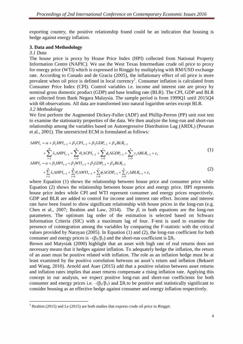
3. Data and Methodology
3.1 Data
The house price is proxy by House Price Index (HPI) collected from National Property
Information Centre (NAPIC). We use the West Texas Intermediate crude oil price to proxy
for energy price (WTI) which is expressed in Ringgit by multiplying with RM/USD exchange
rate. According to Cunado and de Gracia (2005), the inflationary effect of oil price is more
prevalent when oil price is defined in local currency1. Consumer inflation is calculated from
Consumer Price Index (CPI). Control variables i.e. income and interest rate are proxy by
nominal gross domestic product (GDP) and base lending rate (BLR). The CPI, GDP and BLR
are collected from Bank Negara Malaysia. The sample period is from 1999Q1 until 2015Q4
with 68 observations. All data are transformed into natural logarithm series except BLR.
3.2 Methodology
We first perform the Augmented Dickey-Fuller (ADF) and Phillip-Perron (PP) unit root test
to examine the stationarity properties of the data. We then analyze the long-run and short-run
relationship among the variables based on Autoregressive Distribution Lag (ARDL) (Pesaran
et al., 2001). The unrestricted ECM is formulated as follows:
t
s
i
ti
r
i
ti
q
i
ti
p
i
ti
ttttt
BLRGDPCPIHPI
BLRGDPCPIHPIHPI
0
1
0
1
0
1
1
1
14131211
(1)
t
s
iti
r
iti
q
iti
p
iti
ttttt
BLRGDPWTIHPI
BLRGDPWTIHPIHPI
01
01
01
11
14131211
(2)
where Equation (1) shows the relationship between house price and consumer price while
Equation (2) shows the relationship between house price and energy price. HPI represents
house price index while CPI and WTI represent consumer and energy prices respectively.
GDP and BLR are added to control for income and interest rate effect. Income and interest
rate have been found to show significant relationship with house prices in the long-run (e.g.
Chen et al., 2007; Ibrahim and Law, 2014). The βi in both equations are the long-run
parameters. The optimum lag order of the estimation is selected based on Schwarz
Information Criteria (SIC) with a maximum lag of four. F-test is used to examine the
presence of cointegration among the variables by comparing the F-statistic with the critical
values provided by Narayan (2005). In Equation (1) and (2), the long-run coefficient for both
consumer and energy prices is –(β2/β1) and the short-run coefficient is Σθi.
Brown and Matysiak (2000) highlight that an asset with high rate of real returns does not
necessary means that it hedges against inflation. To adequately hedge the inflation, the return
of an asset must be positive related with inflation. The role as an inflation hedge must be at
least examined by the positive correlation between an asset’s return and inflation (Bekaert
and Wang, 2010). Arnold and Auer (2015) add that a positive relation between asset returns
and inflation rates implies that asset returns compensate a rising inflation rate. Applying this
concept in our analysis, we expect positive long-run and short-run coefficients for both
consumer and energy prices i.e. –(β2/β1) and Σθi to be positive and statistically significant to
consider housing as an effective hedge against consumer and energy inflation respectively.
1 Ibrahim (2015) and Le (2015) are both studies that express crude oil price in Ringgit.
Proceedings of 2nd International Conference on Contemporary Economic Issues 2016
5
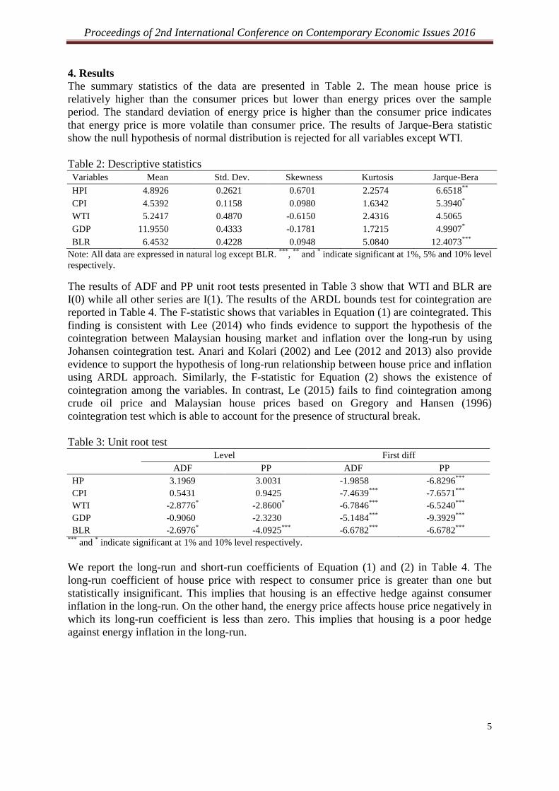
4. Results
The summary statistics of the data are presented in Table 2. The mean house price is
relatively higher than the consumer prices but lower than energy prices over the sample
period. The standard deviation of energy price is higher than the consumer price indicates
that energy price is more volatile than consumer price. The results of Jarque-Bera statistic
show the null hypothesis of normal distribution is rejected for all variables except WTI.
Table 2: Descriptive statistics Variables Mean Std. Dev. Skewness Kurtosis Jarque-Bera
HPI 4.8926 0.2621 0.6701 2.2574 6.6518**
CPI 4.5392 0.1158 0.0980 1.6342 5.3940*
WTI 5.2417 0.4870 -0.6150 2.4316 4.5065
GDP 11.9550 0.4333 -0.1781 1.7215 4.9907*
BLR 6.4532 0.4228 0.0948 5.0840 12.4073***
Note: All data are expressed in natural log except BLR. ***
, **
and * indicate significant at 1%, 5% and 10% level
respectively.
The results of ADF and PP unit root tests presented in Table 3 show that WTI and BLR are
I(0) while all other series are I(1). The results of the ARDL bounds test for cointegration are
reported in Table 4. The F-statistic shows that variables in Equation (1) are cointegrated. This
finding is consistent with Lee (2014) who finds evidence to support the hypothesis of the
cointegration between Malaysian housing market and inflation over the long-run by using
Johansen cointegration test. Anari and Kolari (2002) and Lee (2012 and 2013) also provide
evidence to support the hypothesis of long-run relationship between house price and inflation
using ARDL approach. Similarly, the F-statistic for Equation (2) shows the existence of
cointegration among the variables. In contrast, Le (2015) fails to find cointegration among
crude oil price and Malaysian house prices based on Gregory and Hansen (1996)
cointegration test which is able to account for the presence of structural break.
Table 3: Unit root test
Level First diff
ADF PP ADF PP
HP 3.1969 3.0031 -1.9858 -6.8296***
CPI 0.5431 0.9425 -7.4639***
-7.6571***
WTI -2.8776* -2.8600
* -6.7846
*** -6.5240
***
GDP -0.9060 -2.3230 -5.1484***
-9.3929***
BLR -2.6976* -4.0925
*** -6.6782
*** -6.6782
***
*** and
* indicate significant at 1% and 10% level respectively.
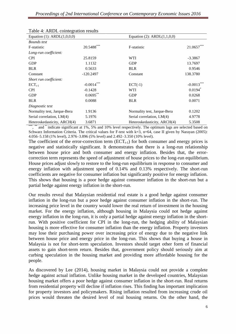
We report the long-run and short-run coefficients of Equation (1) and (2) in Table 4. The
long-run coefficient of house price with respect to consumer price is greater than one but
statistically insignificant. This implies that housing is an effective hedge against consumer
inflation in the long-run. On the other hand, the energy price affects house price negatively in
which its long-run coefficient is less than zero. This implies that housing is a poor hedge
against energy inflation in the long-run.
Proceedings of 2nd International Conference on Contemporary Economic Issues 2016
6
Table 4: ARDL cointegration results Equation (1): ARDL(1,0,0,0)
Equation (2): ARDL(1,1,0,0)
Bounds test
F-statistic 20.5488***
F-statistic 21.0657***
Long-run coefficient:
CPI 25.8159 WTI -3.3867
GDP 1.1132 GDP 13.7697
BLR 0.5633 BLR 0.9546
Constant -120.2497 Constant 138.3780
Short run coefficient:
ECTt-1 -0.0014***
ECT(-1) -0.0013***
CPI -0.1428 WTI 0.0194*
GDP 0.0695**
GDP 0.0268
BLR 0.0088 BLR 0.0071
Diagnostic test
Normality test, Jarque-Bera 1.9136 Normality test, Jarque-Bera 0.1202
Serial correlation, LM(4) 5.1976 Serial correlation, LM(4) 4.9778
Heteroskedasticity, ARCH(4) 3.6871 Heteroskedasticity, ARCH(4) 5.3508 ***
, **
and * indicate significant at 1%, 5% and 10% level respectively. The optimum lags are selected based on
Schwarz Information Criteria. The critical values for F-test with k=3, n=64, case II given by Narayan (2005):
4.056–5.158 (1% level), 2.976–3.896 (5% level) and 2.492–3.350 (10% level). The coefficient of the error-correction term (ECTt-1) for both consumer and energy prices is
negative and statistically significant. It demonstrates that there is a long-run relationship
between house price and both consumer and energy inflation. Besides that, the error-
correction term represents the speed of adjustment of house prices to the long-run equilibrium.
House prices adjust slowly to restore to the long-run equilibrium in response to consumer and
energy inflation with adjustment speed of 0.14% and 0.13% respectively. The short-run
coefficients are negative for consumer inflation but significantly positive for energy inflation.
This shows that housing is a poor hedge against consumer inflation in the short-run but a
partial hedge against energy inflation in the short-run.
Our results reveal that Malaysian residential real estate is a good hedge against consumer
inflation in the long-run but a poor hedge against consumer inflation in the short-run. The
increasing price level in the country would lower the real return of investment in the housing
market. For the energy inflation, although housing in Malaysia could not hedge against
energy inflation in the long-run, it is only a partial hedge against energy inflation in the short-
run. With positive coefficient for CPI in the long-run, the hedging ability of Malaysian
housing is more effective for consumer inflation than the energy inflation. Property investors
may lose their purchasing power over increasing price of energy due to the negative link
between house price and energy price in the long-run. This shows that buying a house in
Malaysia is not for short-term speculation. Investors should target other form of financial
assets to gain short-term return. Besides that, government policy should seriously aim at
curbing speculation in the housing market and providing more affordable housing for the
people.
As discovered by Lee (2014), housing market in Malaysia could not provide a complete
hedge against actual inflation. Unlike housing market in the developed countries, Malaysian
housing market offers a poor hedge against consumer inflation in the short-run. Real returns
from residential property will decline if inflation rises. This finding has important implication
for property investors and policymakers. Rising inflation resulted from increasing crude oil
prices would threaten the desired level of real housing returns. On the other hand, the
Proceedings of 2nd International Conference on Contemporary Economic Issues 2016
7
implementation of Goods and Services Tax (GST) could lead to higher consumer inflation in
the country and seriously impact on the housing returns. The real return from housing
investment may not be well sustained under these circumstances.
5. Conclusion
This study examines the inflation hedging ability of Malaysian residential property by
investigating the relationship between house prices and both consumer and energy prices. We
would like to determine whether residential property in Malaysia is a hedge against consumer
and energy inflation over 1999-2015 periods. From the ARDL results, we find that Malaysian
residential property provides a complete hedge against consumer inflation over the long-term
sample period. However, it is not hedge against energy inflation in the long-run. In the short-
run, housing is able to hedge against energy inflation partially but not the consumer inflation.
Investors should consider both consumer and energy inflation in their decision making
process. Inflation risk arises from increasing oil price could reduce the wealth of property
investors. Investors seeking inflation protection should be aware of the degree of hedging
ability against energy inflation. Malaysian residential property is not a good investment asset
that providing protection on investors’ wealth against energy inflation.
Acknowledgement: Research University Grant Scheme 1001/PSOSIAL/816302 by
Universiti Sains Malaysia is acknowledged.
References
Amonhaemanon, D., De Ceuster, M. J., Annaert, J. and Le Long, H., 2013. The inflation
hedging ability of real estate evidence in Thailand: 1987 - 2011. Procedia Economics and
Finance, 5, 40-49.
Anari, A. and Kolari, J., 2002. House prices and inflation. Real Estate Economics, 30(1), 67-
84.
Arnold, S. and Auer, B. R., 2015. What do scientists know about inflation hedging? North
American Journal of Economics and Finance, 34, 187-214.
Arnott, R. D. and Greer, R. J., 2006. Alternative asset allocation for real return. In R. J. Greer,
The Handbook of Inflation Hedging Investments (pp. 265-282). New York: McGraw-Hill.
Barkham, R. J., Ward, C. R. and Henry, O. T., 1996. The inflation-hedging characteristics of
UK property. Journal of Property Finance, 7(1), 62-76.
Bekaert, G. and Wang, X., 2010. Inflation risk and inflation risk premium. Economic Policy ,
25(64), 755-860.
Beltratti, A. and Morana, C., 2010. International house prices and macroeconomic
fluctuations. Journal of Banking & Finance, 34(3), 533-545.
Bond, M. T. and Seiler, M. J., 1998. Real estate returns and inflation: an added variable
approach. Journal of Real Estate Research, 15(3), 327-338.
Breitenfellner, A., Cuaresma, J. C. and Mayer, P., 2015. Energy inflation and house price
corrections. Energy Economics, 48, 109-116.
Brown, G. and Matysiak, G. A., 2000. Real Estate Investment A Capital Market Approach.
England: Pearson Education Limited.
Chen, M. C., Tsai, I. C. and Chang, C. O., 2007. House prices and household income: Do
they move apart? Evidence from Taiwan. Habitat International, 31, 243-256.
Cunado, J. and de Gracia, F. P., 2005. Oil prices, economic activity and inflation: evidence
for some Asian countries. The Quarterly Review of Economics and Finance, 45, 65-83.
Fama, E. F. and Schewert, G. W., 1977. Asset returns and inflation. Journal of Financial
Economics, 5, 115-146.

Proceedings of 2nd International Conference on Contemporary Economic Issues 2016
8
Frankel, M. S. and Lippmann, J. S., 2006. Real estate as an investment: overview of
alternative vehicles. In R. J. Greer, The Handbook of Inflation Hedging Investments (pp.
179-202). New York: Mc-Graw Hill.
Ganesan, S. and Chiang, Y. H., 1998. The inflation hedging characteristics of real and
financial assets in Hong Kong. Journal of Real Estate Portfolio Management, 4(1), 55-76.
Gregory, A. W. and Hansen, B. E., 1996. Residual-based tests for cointegration in models
with regime shifts. Journal of Econometrics, 70, 99-126.
Ibrahim,I., Sundarasen,S.D. and Ahmad Shayuti,A.F., 2009. Property investment and
inflation hedging in residential property:the case of district of Gombak, Selangor D.E.
The IUP Journal of Applied Finance,15(2), 38-45.
Ibrahim, M. H., 2015. Oil and food prices in Malaysia: a nonlinear ARDL
analysis. Agricultural and Food Economics, 3(1), 1-14.
Ibrahim, M. and Law, S. H., 2014. House prices and bank credits in Malaysia: An aggregate
and disaggregate analysis. Habitat International , 42, 111-120. Kilian, L., 2008. The economic effects of energy price shocks. Journal of Economic
Literature, 46(4), 871-909.
Le, T. H., 2015. Do soaring global oil prices heat up the housing market? Evidence from
Malaysia. Economics: The Open-Access, Open-Assessment E-Journal, 9 (2015-27), 1-30.
Lee, C. L., 2014. The inflation-hedging characteristics of Malaysian residential property.
International Journal of Housing Markets and Analysis, 7(1), 61-75.
Lee, K. N., 2013. A cointegration analysis of inflation and real estate returns. Journal of Real
Estate Portfolio Management, 19(3), 207-223.
Lee, K. N., 2012. Inflation and Residential Property Markets: A Bounds Testing Approach.
International Journal of Trade, Economics and Finance, 3(3), 183-186.
Li, L. H. and Ge, C. L., 2008. Inflation and housing market in Shanghai. Property
Management, 26(4), 273-288.
Narayan, P. K., 2005. The saving and investment nexus for China: evidence from
cointegration tests. Applied Economics, 37(17), 979-1990.
Pesaran, M. H., Shin, Y. and Smith, R. J., 2001. Bounds testing approaches to the analysis of
level relationships. Journal of Applied Econometrics, 16, 289-326.
Rubens, J. H., Bond, M. T. and Webb, J. R., 1989. The inflation-hedging effectiveness of real
estate. Journal of Real Estate Research, 4(2), 45-55.
Shiller, R. J., 2005. Irrational Exuberance (2nd ed.). Princeton University Press.
Sing, T. F. and Low, S. H. 2000. The inflation hedging characteristics of real estate and
financial assets in Singapore. Journal of Real Estate Portfolio Management, 6(4), 373-
385.
Stevenson, S., 2000. A long-term analysis of regional housing markets and inflation. Journal
of Housing Economics, 9, 24-39.
Stevenson, S., 1999. The performance and inflation hedging ability of regional housing
markets. Journal of Property Investment & Finance, 17(3), 239 - 260.
Toda, H. Y. and Yamamoto, T, 1995. Statistical inference in vector autoregressions with
possibly integrated processes. Journal of Econometrics, 66, 225-250.
Tsai, C. L., 2015. How do U.S. stock returns respond differently to oil price shocks pre-crisis,
within the financial crisis, and post-crisis? Energy Economics, 50, 47-62.

Proceedings of 2nd International Conference on Contemporary Economic Issues 2016
9
The Effect of Public Debt on Energy-Growth Nexus:
Threshold Regression Analysis
Sze Wei Yonga,
*, Hooi Hooi Leanb, Jerome Kueh
c
a Faculty of Business & Management, Universiti Teknologi MARA, Sarawak
Email: [email protected]
b School of Social Sciences, Universiti Sains Malaysia
c Faculty of Economics & Business, Universiti Malaysia Sarawak
Abstract
ASEAN countries are dealing with challenging external environment recently with the
deterioration of the global commodity price and the volatility of oil price. Most of the
developing countries rely heavily on the energy consumption for the economic development
purpose especially ASEAN countries which are the major energy exporter like Malaysia and
Indonesia. This study aims to examine the relationship between energy consumption and
economic growth from the perspective of public debt for Indonesia and Malaysia between
periods of 2000 - 2013 via the threshold regression analysis. Our empirical results indicate
that there are significant relationship between energy consumption and economic growth
from the public debt threshold perspective for both countries. The analysis of Indonesia
shows that higher level of public debt will lead to greater impact on energy consumption and
economic nexus. In contrast, the impact of the energy consumption on economic growth for
the case of Malaysia indicates a diminishing trend in the energy and economic growth nexus
when the public debt is above the threshold level. Important policy implication from this
study suggests that Indonesia and Malaysia should be more careful in formulating the energy
consumption related policy by considering different perspectives such as public debt level of
the nation. Moreover, both countries should consider reducing their dependence on the non-
renewable energy resources and shifting to renewable energy resources such as solar, hydro,
landfill gas for their economic development in the future.
Keywords: Energy consumption; economic growth; public debt; threshold regression
analysis.
JEL classification: Q43; O40; H63; C32
1. Introduction
Energy is key resources that contribute to the industrial and economic development in any
nation. The contribution of energy in economy of production can be viewed from demand
and supply perspectives. On the demand side, electricity consumption is one of the form of
energy that used by customer to satisfy their utility. Meanwhile, energy is viewed as vital
factor of production from the supply side to increase the national output and stimulate the
economic growth of a nation (Mathur et. al, 2016). High demand on energy which engaged
in the process of economic development is rising from year to year especially in developing
countries over the last 50 years (Omay et.al, 2015). Developing countries like Association of
Southeast East Asian Nations (ASEAN) member countries are playing essential roles to
influence the trends of world energy consumption. However, most of the ASEAN countries
are dealing with challenging external environment recently with the deterioration of the
global commodity price and the volatility of oil price. These countries rely heavily on the
energy consumption where the energy serves as one of the driver for growth in this region
Proceedings of 2nd International Conference on Contemporary Economic Issues 2016
10
especially those major fossil-fuel producer and exporter like Indonesia and Malaysia.
According to World Energy Outlook Special Report (2015), energy demand of ASEAN
member countries escalated over 50% between 2000-2013. Besides, this report revealed that
Indonesia is the largest energy consumer among the ASEAN member countries as well as the
world largest coal exporter and major liquefied natural gas (LNG). Meanwhile, Malaysia
ranks third largest energy consumer among the ASEAN countries and the world’s second
largest liquefied natural gas (LNG) in 2014 other than the oil exporter.
There are numerous studies on the energy consumption and economic growth nexus. Most of
them suggested that economic growth have significant relationship with energy consumption.
(Ang, 2008; Sharma, 2010; Loganathan et.al, 2010; Mathur, 2016). Nevertheless, there are
some researchers disagreed with this finding. In fact, they indicated that the impact of energy
consumption on economic growth is minimal. (Okonkwo and Gbadebo, 2009 and Noor et.al,
2010).The mixed findings of previous literatures failed to show consensus among the
researchers either on the relationship of energy consumption and economic growth in general
or the direction of causality for these two variables in specific. Most of the previous
literatures study on the short run and long run relation or the direction of causality between
energy consumption and economic growth nexus. There were very few studies examined the
energy consumption and economic growth nexus from other perspectives.
One of the elements that might influence energy consumption and economic growth nexus is
public debt. The swelling of public debt has become an emergence issues after the European
debt crisis. Public debt crises raise the awareness of policy makers on the public debt issue
such as dealing with the risk of credit slowdown and or bust that might affect the economic
growth. Public debt is an important instrument that used to measure the sustainability of the
country’s finances. It reflects the repayment ability of a country to their debtors. High level of
public debt will lead to the financial risk in term of outright default or capital flight.
Moreover, it will also crowd out domestic spending via the escalating of interest risk
premium and limit economic growth (Makin, 2005). Reinhart and Rogoff (2010) stated that
growth performance of country will be deteriorated when public debt surpasses 90% of GDP
threshold level. However, reasonable levels of public debt are likely to enhance its economic
growth by financing productive investment. Therefore, this study aims to investigate the
influence of threshold level of public debt on energy consumption and economic growth
nexus. This paper is differs from other literatures from two aspects. Firstly, this study focuses
on Indonesia and Malaysia through threshold regression model for the period of 2000-2013.
The sample period reflects up-to-date development for Indonesia and Malaysia in 2000s.
Secondly, this study is examining the energy consumption and economic growth nexus from
threshold level of public debt. As per our knowledge, there are hardly to find literatures that
review on the relationship between energy consumption and economic growth from public
debt perspectives. The findings of this paper will provide new insight to the current literatures
as well as to fulfill the existing gaps. The rest of this paper is organized as follows. Section 2
discusses on literature reviews. Section 3explain the data and methods. Section 4 presents the
empirical results and the last section provides conclusion and policy implication.
2. Literature Review
Energy consumption is an eminent issue that has been thoroughly discussed by scholars,
academician, researcher as well as government policy maker over the past decade. There
were numerous empirical literatures on the relationship between energy consumption and
economic growth. Most of the literatures on energy consumption and economic growth nexus
focus on developing countries especially ASEAN region. Ang (2008) examined the
relationship of energy and output of Malaysia for the period of 1971 to 1999 revealed that

Proceedings of 2nd International Conference on Contemporary Economic Issues 2016
11
energy consumption have positive relationship with economic growth in the long run.
Besides, the causality result indicates that economic growth has causal effect on energy
consumption for long run and short run in Malaysia. The case of Malaysia was further
investigated by Loganathan et.al (2010) who discovered the existence of bidirectional co-
integration effects between the total energy consumption and the economic growth of
Malaysia over the period of 1971 to 2008. They applied different methods such as Ordinary
Least Square Engel-Granger (OLS-EG), Dynamic Ordinary Least Square (DOLS),
Autoregressive Distributed Lag (ARDL) Bounds testing approach and Error Correction
Model (ECM) to examine the sustainability of energy consumption and economic
performance of Malaysia. Furthermore, their findings revealed that energy consumption was
on supportable perimeter with 57% speed of adjustment to achieve the long run equilibrium
due to the short run shock in economic growth of Malaysia. Besides the case of Malaysia,
Gross (2012) who study the non-causality between energy and economic growth in the US
for the period of 1970 to 2007 through Granger causality test for three sectors consists of
industry, commercial sector and transport sector. The empirical result shows that there is
unidirectional long run Granger causality in the commercial sector from growth to energy and
bi-directional long-run Granger causality in the transport sector.
On the other hand, some researchers investigated the relationship of energy consumption and
economic growth based on many countries at the same region or different regions such as
Sharma (2010), Apergis and Payne (2010), Razzaqi et. al (2011) and Omay et.al (2015).
Study of Sharma (2010) focus on the linkage between energy consumption and economic
growth for 66 countries across few regions such as Asia Pacific region, Europe and Central
Asian region, Latin America and Caribbean region and sub-Saharan, North Africa and
Middle Eastern region. Dynamic panel data models have been applied in the study and the
result stated that energy consumption (both electricity and non-electricity type energy
variables) has significant relationship with economic growth in Europe and Central Asian
region. Meanwhile, Apergis and Payne (2010) who study on the renewable energy
consumption and economic growth for 20 OECD countries over the period of 1985-2005
provide evidence to show that there are long run significant relationship between energy
consumption and economic growth through panel cointegration test. The Granger causality
test shows that there is bi-directional causality between energy consumption and economic
growth in short run as well as long run. Apparently, their funding was supported by Razzaqi
et. al (2011) who examined on the relationship between energy consumption and economic
growth for developing-8 (D8) countries (Bangladesh, Egypt, Indonesia, Iran, Malaysia,
Nigeria, Pakistan and Turkey) via Johansen’s cointergation test proved that the existence of
dynamic relationship between energy consumption and GDP occur in all D-8 countries.
Moreover, their research also provides the evidence of bi-directional long run causality
between energy consumption and economic growth exist through VECM and VAR causality
test for the case of Indonesia and Malaysia. Another study of Omay et.al (2015) on the
relationship of energy consumption and economic growth for eight developing countries from
Europe and Central Asia (Azerbaijan, Bulgaria, Kzakhstan, Latvia, Lithuania, Romania,
Russia Federation and Turkey) via the non-linear causality test suggested that the existence of
two way relationship running from economic growth to energy consumption. The causality
test revealed that one way causality running from economic growth to energy consumption
was found.
There is another strand of researchers who show their disagreement on the findings of causal
relationship exist between energy consumption and economic growth such as Chiou-Wei et.
al (2011) and Mathur (2016). Chiou Wei et.al (2011) conduct their research based on meta-
Proceedings of 2nd International Conference on Contemporary Economic Issues 2016
12
analysis on the energy consumption and economic growth nexus stated that not all the
developing countries shows the unidirectional causality from energy consumption to
economic growth as compare with developed countries. Their finding was supported by
Mathur (2016) who studied on the energy-growth nexus for 52 countries that consist of 18
developing countries, 16 transition ad 18 developed countries via various panel data
estimation methods such as panel data cointegration, panel causality, panel VECM, panel
VAR and panel data ARDL and SURE. Their result revealed that energy consumption has a
negative impact on the economic growth for developing countries and transitional economies.
In contrast, there are positive effect of energy consumption towards economic growth exists
for the case of developed countries.
3. Data and Medothology
Sample period used in this study covers from 2000:Q1-2013:Q4. Gross domestic product is
the dependent variable whereas energy consumption as independent variable. In addition, the
public debt expressed as percentage of GDP is the threshold variable. All the variables are
obtained from World Development Indicator (WDI).
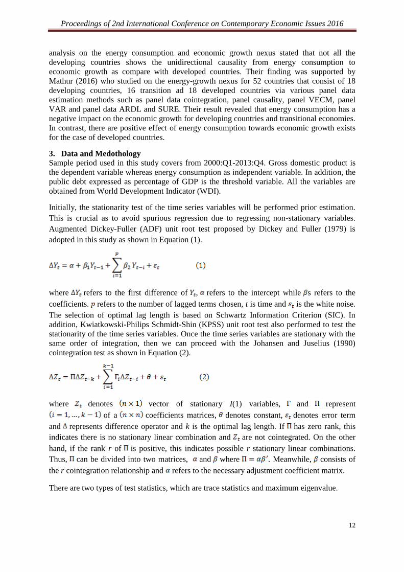
Initially, the stationarity test of the time series variables will be performed prior estimation.
This is crucial as to avoid spurious regression due to regressing non-stationary variables.
Augmented Dickey-Fuller (ADF) unit root test proposed by Dickey and Fuller (1979) is
adopted in this study as shown in Equation (1).
where refers to the first difference of , refers to the intercept while s refers to the
coefficients. refers to the number of lagged terms chosen, t is time and is the white noise.
The selection of optimal lag length is based on Schwartz Information Criterion (SIC). In
addition, Kwiatkowski-Philips Schmidt-Shin (KPSS) unit root test also performed to test the
stationarity of the time series variables. Once the time series variables are stationary with the
same order of integration, then we can proceed with the Johansen and Juselius (1990)
cointegration test as shown in Equation (2).
where denotes vector of stationary I(1) variables, and represent
of a coefficients matrices, denotes constant, denotes error term
and represents difference operator and k is the optimal lag length. If has zero rank, this
indicates there is no stationary linear combination and are not cointegrated. On the other
hand, if the rank r of is positive, this indicates possible r stationary linear combinations.
Thus, can be divided into two matrices, and where . Meanwhile, consists of
the r cointegration relationship and refers to the necessary adjustment coefficient matrix.
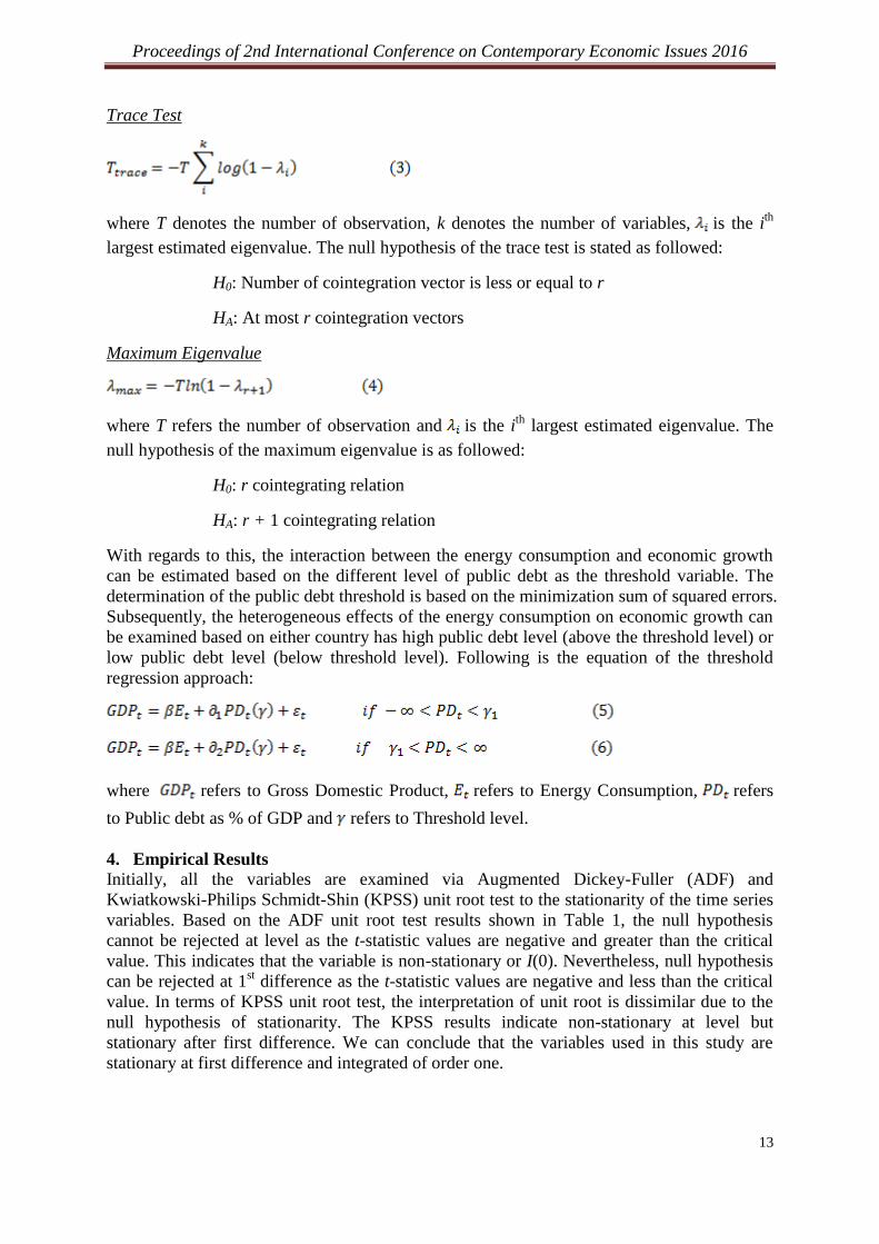
There are two types of test statistics, which are trace statistics and maximum eigenvalue.
Proceedings of 2nd International Conference on Contemporary Economic Issues 2016
13
Trace Test
where T denotes the number of observation, k denotes the number of variables, is the ith
largest estimated eigenvalue. The null hypothesis of the trace test is stated as followed:
H0: Number of cointegration vector is less or equal to r
HA: At most r cointegration vectors
Maximum Eigenvalue
where T refers the number of observation and is the ith
largest estimated eigenvalue. The
null hypothesis of the maximum eigenvalue is as followed:
H0: r cointegrating relation
HA: r + 1 cointegrating relation
With regards to this, the interaction between the energy consumption and economic growth
can be estimated based on the different level of public debt as the threshold variable. The
determination of the public debt threshold is based on the minimization sum of squared errors.
Subsequently, the heterogeneous effects of the energy consumption on economic growth can
be examined based on either country has high public debt level (above the threshold level) or
low public debt level (below threshold level). Following is the equation of the threshold
regression approach:
where refers to Gross Domestic Product, refers to Energy Consumption, refers
to Public debt as % of GDP and refers to Threshold level.
4. Empirical Results
Initially, all the variables are examined via Augmented Dickey-Fuller (ADF) and
Kwiatkowski-Philips Schmidt-Shin (KPSS) unit root test to the stationarity of the time series
variables. Based on the ADF unit root test results shown in Table 1, the null hypothesis
cannot be rejected at level as the t-statistic values are negative and greater than the critical
value. This indicates that the variable is non-stationary or I(0). Nevertheless, null hypothesis
can be rejected at 1st difference as the t-statistic values are negative and less than the critical
value. In terms of KPSS unit root test, the interpretation of unit root is dissimilar due to the
null hypothesis of stationarity. The KPSS results indicate non-stationary at level but
stationary after first difference. We can conclude that the variables used in this study are
stationary at first difference and integrated of order one.
Proceedings of 2nd International Conference on Contemporary Economic Issues 2016
14
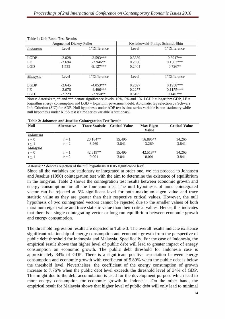
Table 1: Unit Roots Test Results
Augmented Dickey-Fuller Kwiatkowski-Philips Schmidt-Shin
Indonesia
Level 1stDifference Level 1
stDifference
LGDP -2.028 -3.593*** 0.3339 0.3917**
LE -2.694 -2.946** 0.2050 0.1503***
LGD 1.535 -9.127*** 0.2401 0.7267*
Malaysia
Level 1stDifference Level 1
stDifference
LGDP -2.645 -4.053*** 0.2697 0.1958***
LE -2.676 -4.496*** 0.2257 0.1155***
LGD -2.229 -2.950** 0.5105 0.1402**
Notes: Asterisks *, ** and *** denote significance levels: 10%, 5% and 1%. LGDP = logarithm GDP, LE =
logarithm energy consumption and LGD = logarithm government debt. Automatic lag selection by Schwarz
Info Criterion (SIC) for ADF. Null hypothesis under ADF test is time series variable is non-stationary while
null hypothesis under KPSS test is time series variable is stationary.
Table 2: Johansen and Juselius Cointegration Test Result
Null Alternative Trace Statistic Critical Value Max-Eigen
Value
Critical Value
Indonesia
r = 0 r = 1 20.164** 15.495 16.895** 14.265
r < 1 r = 2 3.269 3.841 3.269 3.841
Malaysia
r = 0 r = 1 42.519** 15.495 42.518** 14.265
r < 1 r = 2 0.001 3.841 0.001 3.841
Asterisk ** denotes rejection of the null hypothesis at 0.05 significance level.
Since all the variables are stationary or integrated at order one, we can proceed to Johansen
and Juselius (1990) cointegration test with the aim to determine the existence of equilibrium
in the long-run. Table 2 shows the cointegration test results between economic growth and
energy consumption for all the four countries. The null hypothesis of none cointegrated
vector can be rejected at 5% significant level for both maximum eigen value and trace
statistic value as they are greater than their respective critical values. However, the null
hypothesis of two cointegrated vectors cannot be rejected due to the smaller values of both
maximum eigen value and trace statistic value than their critical values. Hence, this indicates
that there is a single cointegrating vector or long-run equilibrium between economic growth
and energy consumption.
The threshold regression results are depicted in Table 3. The overall results indicate existence
significant relationship of energy consumption and economic growth from the perspective of
public debt threshold for Indonesia and Malaysia. Specifically, For the case of Indonesia, the
empirical result shows that higher level of public debt will lead to greater impact of energy
consumption on economic growth. The public debt threshold for Indonesia case is
approximately 34% of GDP. There is a significant positive association between energy
consumption and economic growth with coefficient of 5.89% when the public debt is below
the threshold level. Nevertheless, the coefficient of the energy consumption of growth
increase to 7.76% when the public debt level exceeds the threshold level of 34% of GDP.
This might due to the debt accumulation is used for the development purpose which lead to
more energy consumption for economic growth in Indonesia. On the other hand, the
empirical result for Malaysia shows that higher level of public debt will only lead to minimal
Proceedings of 2nd International Conference on Contemporary Economic Issues 2016
15
impact on the energy consumption and economic growth nexus. In the case of Malaysia, the
public debt threshold is approximately 52% of GDP. There is a declining effect from 2.89%
to 1.68% of energy consumption on growth when the public debt is above the threshold level.
This might due to not all public debt is used for the development purpose but used for debt
repayment. The empirical result shows the existence of significant relationship between
energy consumption and economic growth for the case of Indonesia and Malaysia is
consistent with the findings of Ang (2008), Loganathan et.al (2010) and Razzaqi et.al (2011).
This signified that public debt play certain roles in both countries to influence the energy
consumption and growth nexus especially Indonesia.
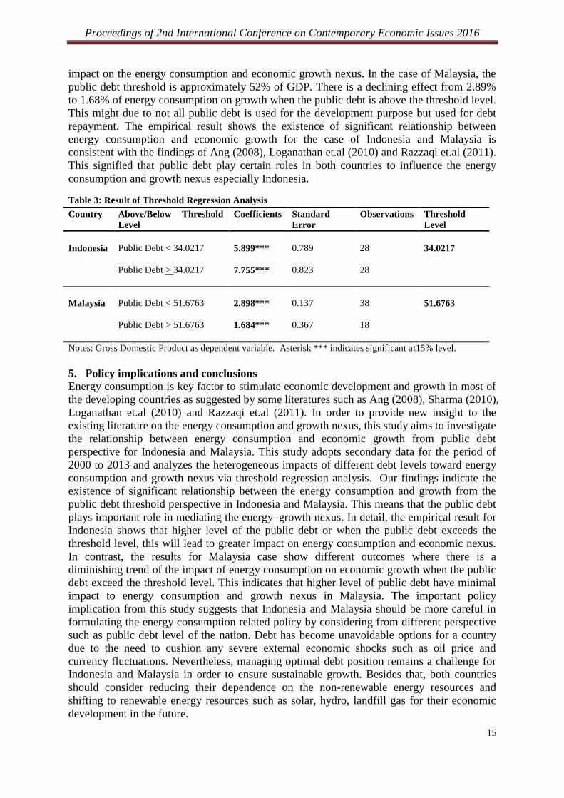
Table 3: Result of Threshold Regression Analysis
Country Above/Below Threshold
Level
Coefficients Standard
Error
Observations Threshold
Level
Indonesia
Public Debt < 34.0217
5.899***
0.789
28
34.0217
Public Debt > 34.0217 7.755***
0.823 28
Malaysia
Public Debt < 51.6763
2.898***
0.137
38
51.6763
Public Debt > 51.6763 1.684***
0.367 18
Notes: Gross Domestic Product as dependent variable. Asterisk *** indicates significant at15% level.
5. Policy implications and conclusions
Energy consumption is key factor to stimulate economic development and growth in most of
the developing countries as suggested by some literatures such as Ang (2008), Sharma (2010),
Loganathan et.al (2010) and Razzaqi et.al (2011). In order to provide new insight to the
existing literature on the energy consumption and growth nexus, this study aims to investigate
the relationship between energy consumption and economic growth from public debt
perspective for Indonesia and Malaysia. This study adopts secondary data for the period of
2000 to 2013 and analyzes the heterogeneous impacts of different debt levels toward energy
consumption and growth nexus via threshold regression analysis. Our findings indicate the
existence of significant relationship between the energy consumption and growth from the
public debt threshold perspective in Indonesia and Malaysia. This means that the public debt
plays important role in mediating the energy–growth nexus. In detail, the empirical result for
Indonesia shows that higher level of the public debt or when the public debt exceeds the
threshold level, this will lead to greater impact on energy consumption and economic nexus.
In contrast, the results for Malaysia case show different outcomes where there is a
diminishing trend of the impact of energy consumption on economic growth when the public
debt exceed the threshold level. This indicates that higher level of public debt have minimal
impact to energy consumption and growth nexus in Malaysia. The important policy
implication from this study suggests that Indonesia and Malaysia should be more careful in
formulating the energy consumption related policy by considering from different perspective
such as public debt level of the nation. Debt has become unavoidable options for a country
due to the need to cushion any severe external economic shocks such as oil price and
currency fluctuations. Nevertheless, managing optimal debt position remains a challenge for
Indonesia and Malaysia in order to ensure sustainable growth. Besides that, both countries
should consider reducing their dependence on the non-renewable energy resources and
shifting to renewable energy resources such as solar, hydro, landfill gas for their economic
development in the future.

Proceedings of 2nd International Conference on Contemporary Economic Issues 2016
16
References
Ang J.B., 2008. Economic Development, Pollutant Emissions and Energy Consumption in
Malaysia. Journal of Policy Modelling. 30, 271-8.
Apergis, N. and Payne, J.E., 2010. Renewable Energy Consumption and Economic Growth:
Evidence from a panel of OECD countries. Energy Policy. 38 (2010) 656-660.
Chiou Wei, S.Z. and Ko, C. C., 2011. A Meta-Analysis of the Relationships between Energy
Consumption and Economic Growth. Conference Proceeding Paper.528-545.
Dickey, D. and Fuller, W., 1979. Distribution of the Estimators for Autoregressive Time
Series with a Unit Root. Journal of American Statistical Association. 74, 427-431.
Gross, C., 2012. Explaining the (non-) causality between energy and economic growth in the
U.S.- A multivariate sectoral analysis. Energy Economics. 34, 489-499.
International Energy Agency & Economic Research Institute for ASEAN and East Asia.
2015. Southeast Asia Energy Outlook 2015. World Energy Outlook Special Report.
http://www.worldenergyoutlook.org. Assessed 31July 2016.
Johansen, S. and Juselius, K. 1990, Maximum Likelihood Estimation and Inference in
Cointegration with Applications for Demand for Money, Oxford Bulletin Economic
Statistics, 52, 169-210.
Loganathan, Nanthakumar and Subramaniam, T., 2010. Dynamic Cointegration Link
between Energy consumption and Economic Performance: Empirical Evidence from
Malaysia. International Journal of Trade. Economics and Finance 1:3.
Makin, A.J., 2005. Public debt Sustainability and Its Macroeconomic Implications in ASEAN
4. ASEAN Economic Bulletin, 22(3), 284-96.
Mathur, S.K., Sahu.S., Thorat I.G. and Aggarwal, 2016. Does Domestic Energy
Consumption affect GDP of a Country? A Panel Data Study. Global Economy Journal.
16(2): 229-273.
Noor, S. and Siddiqi, M.W., 2010. Energy Consumption and Economic Growth in South
Asian Countries: A Co-integrated Panel Analysis. International Journal of Human and
Social Sciences 5(14).
Okonkwo, C. and Gradebo, O. 2009. Does Energy Consumption Contribute to Economic
Performance? Empirical Evidence from Nigeria. Journal of Economics and Business.
12(2).
Omay, T., Apergis, N. and Ozcelebi, H., 2015. Energy Consumption and Growth: New
Evidence from a Non- Linear Panel and a sample of Developing Countries. The
Singapore Economic Review. 60(2). 155018-1-1550018-60.
Razzaqi, S., Bilquees, F. and Sherbaz, S., 2011. Dynamic relationship between Energy and
Economic Growth: Evidence from D8 Countries. The Pakistan Development Review.
50(4). 437-458.
Reinhart, C.M. and Rogoff, K.S., 2010. Growth in a Time of Debt, National Bureau of
Economic Research Working Paper Series.
Sharma, S.S., 2010. The relationship between energy and economic growth: Empirical
evidence from 66 countries. Applied Energy. 87, 3565-3574.

Proceedings of 2nd International Conference on Contemporary Economic Issues 2016
17
Estimation of Malaysia Public Debt Threshold
Jerome Kueh1, Venus Khim-Sen Liew
1, Sze-Wei Yong
2,
Muhammad Asraf Abdullah1
1Faculty of Economics and Business, Universiti Malaysia Sarawak, Sarawak, Malaysia
2Faculty of Business & Management, Universiti Teknologi MARA Sarawak, Sarawak,
Malaysia
Abstract
The objective of this study is to examine the implication of the public debt on the economic
growth of Malaysia from the perspective of different public debt levels threshold. Threshold
Regression method is utilized to identify the public debt threshold from 1991:Q1-2014:Q4
and examine the heterogeneous impacts of the public debt on growth based on certain
threshold levels. Empirical results indicate that there is a positive association between the
public debt and economic growth when the public debt is below 41% of GDP threshold level.
Furthermore, there is a marginal positive impact when the public debt level falls between
41%-53% of GDP threshold levels. However, there is a harmful impact on growth when
public debt is above 53% of GDP threshold level. As a result, managing the public debt
position and the quality of the debt are important to ensure sustainable economic growth.
Keywords: Public debt; threshold; growth
JEL Classification: H63, C24, O10
1. Introduction
Debt is unavoidable and is viewed as a tool to curtail the adverse impacts of economic shock.
In the inter-temporal perspective, a country may run into deficit and leads to accumulation of
debt in the circumstances of economic shock with the purpose to mitigate the negative
impacts of the shock. This is with the assumption that the country will experience surplus in
the future due to the recovering of the economy. Nevertheless, the debt level of most of the
countries are showing rising trend and can be harmful to the economic growth of the
countries. For instance, Reinhart and Rogoff (2010) indicate that the threshold of the public
debt is 90% of GDP where countries may experience positive economic growth when the
public debt level is below 90% of GDP threshold level. However, economic growth of the
countries may worsen when the public debt of the countries is beyond the 90% of GDP
threshold level. Therefore, this indicates that the implication of the debt on the economic
growth may diverge depending on the threshold levels.
Malaysia recorded remarkable gross domestic product (GDP) growth in the 1990s with
average 9.2% from 1990 until 1997 (World Economic Outlook, IMF). However, the
economic growth deteriorated drastically due to the Asian Financial crisis in 1997. The
economic growth of Malaysia preserves at the range 4-5% from 2011 to 2014 and recorded
around 4.9% in 2015 (World Economic Outlook, IMF) due to the prudent fiscal and monetary
policies in safeguarding rapid recovery of the economy.
Proceedings of 2nd International Conference on Contemporary Economic Issues 2016
18
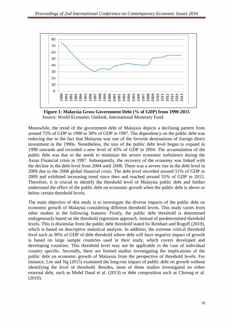
Figure 1: Malaysia Gross Government Debt (% of GDP) from 1990-2015
Source: World Economic Outlook, International Monetary Fund.
Meanwhile, the trend of the government debt of Malaysia depicts a declining pattern from
around 75% of GDP in 1990 to 30% of GDP in 1997. The dependency on the public debt was
reducing due to the fact that Malaysia was one of the favorite destinations of foreign direct
investment in the 1990s. Nonetheless, the size of the public debt level began to expand in
1998 onwards and recorded a new level of 43% of GDP in 2004. The accumulation of the
public debt was due to the needs to minimize the severe economic turbulence during the
Asian Financial crisis in 1997. Subsequently, the recovery of the economy was linked with
the decline in the debt level from 2004 until 2008. There was a severe rise in the debt level in
2009 due to the 2008 global financial crisis. The debt level recorded around 51% of GDP in
2009 and exhibited increasing trend since then and reached around 55% of GDP in 2015.
Therefore, it is crucial to identify the threshold level of Malaysia public debt and further
understand the effect of the public debt on economic growth when the public debt is above or
below certain threshold levels.
The main objective of this study is to investigate the diverse impacts of the public debt on
economic growth of Malaysia considering different threshold levels. This study varies from
other studies in the following features: Firstly, the public debt threshold is determined
endogenously based on the threshold regression approach, instead of predetermined threshold
levels. This is dissimilar from the public debt threshold stated by Reinhart and Rogoff (2010),
which is based on descriptive statistical analysis. In addition, the extreme critical threshold
level such as 90% of GDP of debt threshold where debt will have negative impact of growth
is based on large sample countries used in their study, which covers developed and
developing countries. This threshold level may not be applicable in the case of individual
country specific. Secondly, there are limited studies investigating the implications of the
public debt on economic growth of Malaysia from the perspective of threshold levels. For
instance, Lee and Ng (2015) examined the long-run impact of public debt on growth without
identifying the level of threshold. Besides, most of those studies investigated on either
external debt, such as Mohd Daud et al. (2013) or debt composition such as Choong et al.
(2010).
Proceedings of 2nd International Conference on Contemporary Economic Issues 2016
19
The remainder of the paper is organized as follows: section two provides literature review on
public debt and growth, followed by section three discussing the methodology, section four
provides empirical findings and discussion and last section is conclusion.
2. Literature Review
The impact of the debt on economic growth can be associated to debt overhang hypothesis.
This hypothesis states that there is no incentive for the government to implement
macroeconomic policies to stimulate the economy if a country has high level of debt. This is
due to the yields of successful policies will shift to finance the high level of debt, in terms of
debt interest payment (Clements et al., 2003). Subsequently, the empirical findings provide
mixed conclusion on the effect of debt on growth.
Choong et al. (2010) investigated the impact of various type of debt on economic growth of
Malaysia from 1970 to 2006 using cointegration test and Granger causality test. Empirical
findings indicated that existence of negative impact of the external debt on growth in the
long-run. Meanwhile, Mohd Daud et al. (2013) examined the association between external
debt and economic growth of Malaysia from 1991:Q1 to 2009:Q4 using Autoregressive
Distributed Lag (ARDL). They further estimate the threshold effect via Hansen (2000)
threshold method. The findings indicated that accumulation of external debt is link to
expansion in economic growth of Malaysia until level of RM170,757. This means that there
will be opposite association between external debt and growth when the external debt is
above the threshold level. Lee and Ng (2015) examined the effect of the public debt towards
economic growth of Malaysia for the sample period of 1991-2013. Their findings showed
that public debt has negative impact on the economic growth with coefficient of 1.17%.
In terms of non-linearity perspective, there are several studies emphasize on the turning point
of the debt effect on growth, particularly external debt. For instance, Pattilio et al. (2004)
examined 93 developing countries for a sample period of 1969-1998. Their findings indicated
that the impact of debt on growth become negative when debt level exceed 160-170% of
export and 35-40% of GDP. Meanwhile, Kumar and Woo (2010) investigated the debt effect
on growth for advanced and emerging economies from 1970-2007. Empirical results
indicated that there is an inverse between initial debts on growth with 0.2% point for
advanced countries and 0.15% point for emerging countries upon 10% point increase in
initial debts. Furthermore, there is also evidence of non-linearity where negative effect of
debt on growth when the public debt level is beyond 90% of GDP threshold level. Baum et al.
(2013) investigated the implication of the public debt and economic growth based on sample
countries of 12 Euro area countries from 1990 to 2010. Their empirical findings indicated
that debt contributed positively to the economic growth when the debt is below 67% of GDP
threshold level. Spilioti and Vamvoukus (2015) examined the relationship between debt and
economic growth for Greece from 1970 to 2010. They discovered that debt becomes
detrimental to economic growth when the debt is above 110% of GDP threshold level.
3. Methodology
The data used in this study comprises of gross domestic product per capita expressed in US
dollar and public debt expressed as % of GDP covering the sample period of 1991:Q1 to
2014:Q4. All the variables are obtained from World Economic Outlook, International
Monetary Fund. Initially, this study performs stationarity test on the variables to examine the
order of integration in order to avoid spurious regression. The Augmented Dickey-Fuller
(ADF) unit root test is applied to test the time series properties. Equation (1) shows the
equation for the ADF test.
Proceedings of 2nd International Conference on Contemporary Economic Issues 2016
20
where refers to variable of interest, refers to differencing operator, t refers to time trend
and refers to the error term. The non-rejection of the null hypothesis indicates that has
unit root or non-stationary. On the other hand, the rejection of the null hypothesis indicates
that is stationary.
Cointegration test can be performed if the time series variables are stationary and integrated
in the same order or I(1). The purpose of the cointegration test is to determine the existence
of the long-run equilibrium between the parameters of interest. The Johansen and Juselius
(1990) cointegration test is represented in Equation (2).
where is column vector of stationary I(1) variables, and denote coefficients matrices,
is constant, is error term and is difference operator and k is the optimal lag length. If
has zero rank, there is no stationary linear combination and this indicates that are not
cointegrated. In contrast, if the rank r of is greater than zero, there is possible r stationary
linear combinations. can be divided into two matrices, and where . In detail,
consists of the r cointegration relationship and denotes the necessary adjustment
coefficient matrix.
Johansen and Juselius (1990) introduced two types of test statistics, which are trace statistics
and maximum eigenvalue. In terms of trace statistic, the null hypothesis of r cointegrating
vector while the alternative hypothesis of k cointegrating vector for r = 0, 1, …, k – 1. The
trace statistic test is computed as in Equation (3).
where T denotes the number of observation, k denotes the number of variables, is the i
th
largest estimated eigenvalue.
The maximum eigenvalue statistic examines the null hypothesis of r cointegrating vector
against alternative hypothesis of r + 1 cointegrating vector. The maximum eigenvalue
statistic test is computed as in Equation (4).
where T refers the number of observation and is the i
th largest estimated eigenvalue.
The threshold regression model includes non-linear regression estimation and regime
switching with the aim to capture the interaction between parameters of interest when the
variables exceed certain unknown threshold level.
Following is the equation on the threshold regression approach:
where = Gross Domestic Product per capita, = Public debt as % of GDP, =
Threshold variable
Proceedings of 2nd International Conference on Contemporary Economic Issues 2016
21
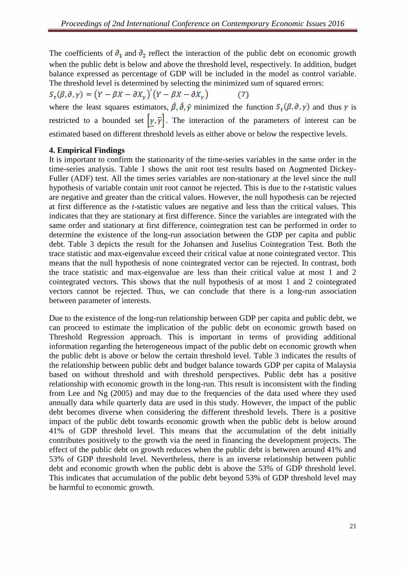
The coefficients of and reflect the interaction of the public debt on economic growth
when the public debt is below and above the threshold level, respectively. In addition, budget
balance expressed as percentage of GDP will be included in the model as control variable.
The threshold level is determined by selecting the minimized sum of squared errors:
where the least squares estimators, minimized the function and thus is
restricted to a bounded set . The interaction of the parameters of interest can be
estimated based on different threshold levels as either above or below the respective levels.
4. Empirical Findings
It is important to confirm the stationarity of the time-series variables in the same order in the
time-series analysis. Table 1 shows the unit root test results based on Augmented Dickey-
Fuller (ADF) test. All the times series variables are non-stationary at the level since the null
hypothesis of variable contain unit root cannot be rejected. This is due to the t-statistic values
are negative and greater than the critical values. However, the null hypothesis can be rejected
at first difference as the t-statistic values are negative and less than the critical values. This
indicates that they are stationary at first difference. Since the variables are integrated with the
same order and stationary at first difference, cointegration test can be performed in order to
determine the existence of the long-run association between the GDP per capita and public
debt. Table 3 depicts the result for the Johansen and Juselius Cointegration Test. Both the
trace statistic and max-eigenvalue exceed their critical value at none cointegrated vector. This
means that the null hypothesis of none cointegrated vector can be rejected. In contrast, both
the trace statistic and max-eigenvalue are less than their critical value at most 1 and 2
cointegrated vectors. This shows that the null hypothesis of at most 1 and 2 cointegrated
vectors cannot be rejected. Thus, we can conclude that there is a long-run association
between parameter of interests.
Due to the existence of the long-run relationship between GDP per capita and public debt, we
can proceed to estimate the implication of the public debt on economic growth based on
Threshold Regression approach. This is important in terms of providing additional
information regarding the heterogeneous impact of the public debt on economic growth when
the public debt is above or below the certain threshold level. Table 3 indicates the results of
the relationship between public debt and budget balance towards GDP per capita of Malaysia
based on without threshold and with threshold perspectives. Public debt has a positive
relationship with economic growth in the long-run. This result is inconsistent with the finding
from Lee and Ng (2005) and may due to the frequencies of the data used where they used
annually data while quarterly data are used in this study. However, the impact of the public
debt becomes diverse when considering the different threshold levels. There is a positive
impact of the public debt towards economic growth when the public debt is below around
41% of GDP threshold level. This means that the accumulation of the debt initially
contributes positively to the growth via the need in financing the development projects. The
effect of the public debt on growth reduces when the public debt is between around 41% and
53% of GDP threshold level. Nevertheless, there is an inverse relationship between public
debt and economic growth when the public debt is above the 53% of GDP threshold level.
This indicates that accumulation of the public debt beyond 53% of GDP threshold level may
be harmful to economic growth.
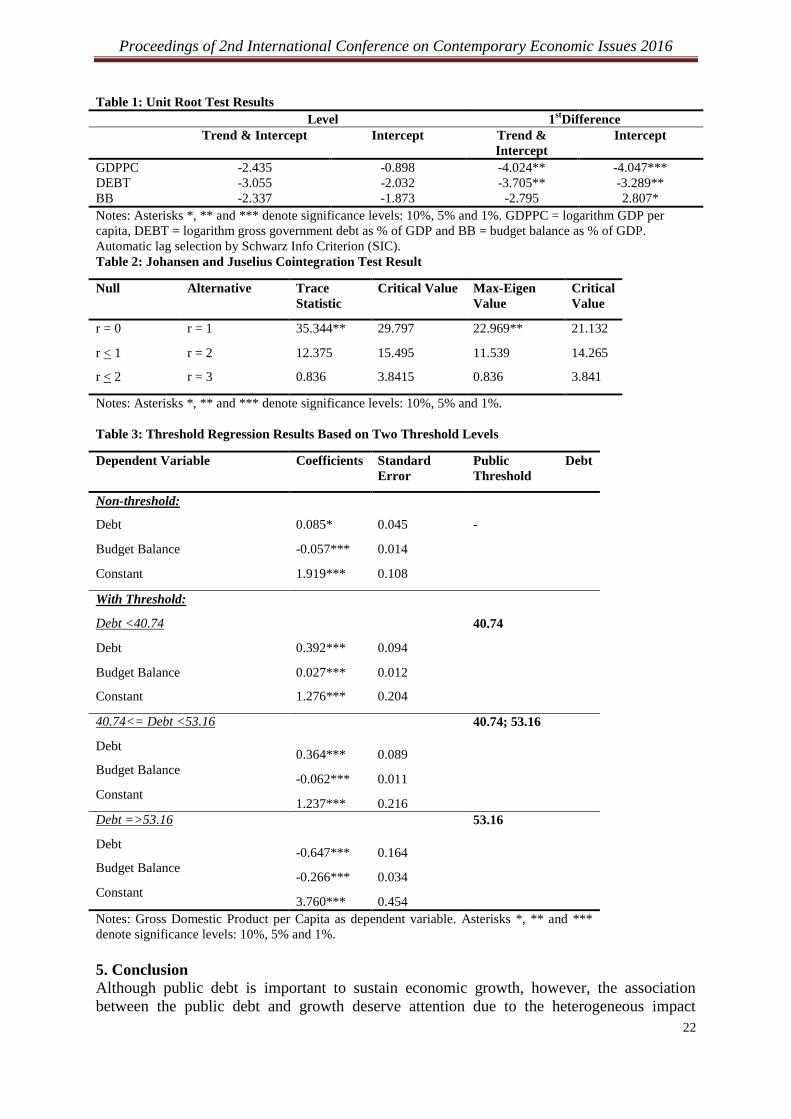
Proceedings of 2nd International Conference on Contemporary Economic Issues 2016
22
Table 1: Unit Root Test Results
Level 1stDifference
Trend & Intercept Intercept Trend &
Intercept
Intercept
GDPPC -2.435 -0.898 -4.024** -4.047***
DEBT -3.055 -2.032 -3.705** -3.289**
BB -2.337 -1.873 -2.795 2.807*
Notes: Asterisks *, ** and *** denote significance levels: 10%, 5% and 1%. GDPPC = logarithm GDP per
capita, DEBT = logarithm gross government debt as % of GDP and BB = budget balance as % of GDP.
Automatic lag selection by Schwarz Info Criterion (SIC).
Table 2: Johansen and Juselius Cointegration Test Result
Null Alternative Trace
Statistic
Critical Value Max-Eigen
Value
Critical
Value
r = 0 r = 1 35.344** 29.797 22.969** 21.132
r < 1 r = 2 12.375 15.495 11.539 14.265
r < 2 r = 3 0.836 3.8415 0.836 3.841
Notes: Asterisks *, ** and *** denote significance levels: 10%, 5% and 1%.
Table 3: Threshold Regression Results Based on Two Threshold Levels
Dependent Variable Coefficients Standard
Error
Public Debt
Threshold
Non-threshold:
Debt 0.085* 0.045 -
Budget Balance -0.057*** 0.014
Constant 1.919*** 0.108
With Threshold:
Debt <40.74 40.74
Debt 0.392*** 0.094
Budget Balance 0.027*** 0.012
Constant 1.276*** 0.204
40.74<= Debt <53.16 40.74; 53.16
Debt 0.364*** 0.089
Budget Balance -0.062*** 0.011
Constant 1.237*** 0.216
Debt =>53.16 53.16
Debt -0.647*** 0.164
Budget Balance -0.266*** 0.034
Constant 3.760*** 0.454
Notes: Gross Domestic Product per Capita as dependent variable. Asterisks *, ** and ***
denote significance levels: 10%, 5% and 1%.
5. Conclusion
Although public debt is important to sustain economic growth, however, the association
between the public debt and growth deserve attention due to the heterogeneous impact

Proceedings of 2nd International Conference on Contemporary Economic Issues 2016
23
depending on the different public debt threshold levels. In the case of Malaysia, there is
positive relationship between public debt and economic growth when the public debt is below
around 41% of GDP threshold level. In addition, the effects weaken when the public debt
level is around 41% to 53% of GDP threshold levels. In contrast, there is an inverse
association between public debt and economic growth when the public debt level exceeds
around 53% of GDP threshold level. This means that the preliminary accumulation of the
public debt leads to the growth of the economy. Nevertheless, additional debt will be harmful
to the economic growth when the debt reaches the optimum level. This is essential to the
policy maker in developing strategies as the impact of public debt on growth differ when the
public debt is above or below certain threshold level.
In terms of policy perspective, managing optimal debt position is crucial for Malaysia in
order to overcome the external economic uncertainties such as oil price fluctuation and
fluctuation in the exchange rate. Besides, the quality of the debt deserve serious attention as
the accumulation of the debt must be compensated with favorable yield in the future.
Therefore, policy developed should monitor closely the public debt level in order to ensure
optimal debt position and the quality of the debt.
Acknowledgement
Financial support from UNIMAS F01/SpGS/1415/16/16 is gratefully acknowledged. All
remaining flaws are the responsibility of the authors.
References
Baum, A., Checherita, C. and Rother, P., 2012. Debt and Growth: New Evidence for the Euro
Area, Journal of International Money and Finance, 32, pp.809-821.
Choong, C.K., E. Lau, K.S.V. Liew and Puah, C.H., 2010. Does Debts Foster Economic
Growth? The Experience of Malaysia, African Journal of Business Management, 8(4):
pp.1564-1575.
Dickey, D. and Fuller, W., 1979. Distribution of the Estimators for Autoregressive Time
Series with a Unit Root, Journal of American Statistical Association, 74, pp.427-431.
Hansen, B., 2000. Sample Splitting and Threshold Estimation, Econometrica, 68, 3, pp.575-
603.
Johansen, S. and Juselius, K., 1990. Maximum Likelihood Estimation and Inference on
Cointegration with Applications for Demand for Money, Oxford Bulletin Economic
Statistics, 52, pp.169-210.
Kumar, M. and Woo, J., 2010. Public Debt and Growth, IMF Working Paper 10/174.
Lee, S.P. and Ng, Y.L., 2015, Public Debt and Economic Growth in Malaysia, Asian
Economic and Financial Review, 5 (1), pp.119-126.
Mohd Daud, S.N., A.H. Ahmad and Azman-Saini, W.N.W., 2013. Does External Debt
Contribute to Malaysia Economic Growth? Economic Research, 26(2): pp.51-68.
Pattilo, C., Poirson, H. and Ricci, L., 2004. What are the Channels through which External
Debt Affects Growth? IMF Working Paper No. 04/15.
Reinhart, C.M. and Rogoff, K.S., 2010. Growth in a Time of Debt, National Bureau of
Economic Research Working Paper Series.
Spilioti, S. and Vamvoukus, G., 2015, The Impact of Government Debt on Economic Growth:
An Empirical Investigation of the Greek Market, The Journal of Economic Asymmetries,
12, pp.34-40.

Proceedings of 2nd International Conference on Contemporary Economic Issues 2016
24
Energy Subsidy and Economic Production: The Evidence from Malaysia
and Indonesia
¹Dzul Hadzwan Husaini a,
*, Hooi Hooi Leanb and Jerome Kueh
a
a Faculty of Economics and Business, Universiti Malaysia Sarawak
Email: [email protected]
b Economics Program, School of Social Sciences, Universiti Sains Malaysia
Abstract
Energy subsidy policy is one of the most favorable policies implemented by many oil
producer countries in improving their economic development. However, the economic
outcome is still debatable due to the implications on economic efficiency, fiscal policy and et
cetera. As two main oil producer countries in ASEAN 5, both Malaysia and Indonesia had
allocated 5% of energy subsidy (% of GDP) averagely throughout the period of 1990-2014.
This paper is intended to study the impact of energy subsidy on economic production in
Malaysia and Indonesia by employing a dynamic panel data analysis. Our finding suggests
that the energy subsidy affects the growth output positively in the long run. We conclude that
energy subsidy is significant to promote economic growth in both countries. The absence of
energy subsidy will bring harm to the economic growth. However, if a reduction of energy
subsidy is essential to improve efficiency and fiscal pressure, we suggest the policymaker to
implement some offsetting policies to cushion the economy from any shocks.
Keywords: Energy; subsidy; output; panel data analysis
1. Introduction
Malaysia and Indonesia are the net oil exporting countries in ASEAN 5. Accumulatively,
they have recorded -117 average value of net energy import throughout 2010-2013. As part
of the oil production countries in the world, Malaysia and Indonesia earned averagely 5.8%
and 2.4% of oil rent (% of GDP) throughout 2010-2014. Tellingly, their revenue was
contributed much by oil production. With the combination of GDP, they have contributed
about 52% share of GDP in ASEAN 5 economies for the year 2014. In addition, both
Malaysia and Indonesia have achieved the highest economic growth in ASEAN 5 economies
which is about 6% and 5% in the year 2014, respectively. Malaysia and Indonesia have
allocated a huge amount of subsidy, about 74% share of total subsidies in ASEAN 5
economies were contributed by Malaysia and Indonesia in 2014. Out of this value, 74% were
allocated for energy subsidy2. In general, as the oil producer countries in the world, it gives
them many advantages to invest much on energy subsidy to drive a good performance of their
macroeconomics and to increase the economic welfare.
There are many arguments on the role of subsidy in promoting economic growth recently. In
one side, it is believed that the subsidy can give a cost advantage to the producer and increase
the economic welfare of a society in the market (Van Beers and Van den Bergh, 2001).
Consequently, it forms a conducive economic environment to promote a rapid national
growth. On the other side, the subsidy program is believed not to form a conducive economic
environment derived from the existence of the death weight loss in the market and fiscal
pressure problem. Thus, it brings to a situation of where the economic system is unproductive
to encourage a rapid national growth (Isaak, 2015; Arzedel Granado et al, 2012). In respect to
2 All numbers and percentage quoted are retrieved from World Bank Development Indicator (WDI), Bank
Negara Malaysia and Bank Sentral Republik Indonesia.

Proceedings of 2nd International Conference on Contemporary Economic Issues 2016
25
this matter, the government has initiated to rationalize its subsidy policy to ensure that the
subsidy becomes a productive tool to promote growth and reduce its fiscal pressure,
concurrently. One aggressive action that has been taken is that to reduce significant amount
to be allocated for energy subsidy. To date, Indonesia had managed to reduce its subsidy
growth about -85% derived from its initiatives to reduce 148% growths for energy subsidy in
2015. Same as Malaysia, it managed to reduce 16% of its subsidy growth derived from a
reduction of 9% growth for energy subsidy in 2014. As both economies are highly dependent
on subsidy, specifically energy subsidy, this policy will definitely affect their economic
activity as a whole via various channels.
In regards to this matter, we argue that it is important for the current literature to discover the
impact of economic shock derives from the absence of energy subsidy in an economy toward
the sustainable growth of macroeconomic performance. Thus, this paper is intended to
explore the long run impact of energy subsidy on economic output by employing the dynamic
panel data analysis. The objective of this paper is to determine the long-run impact of energy
subsidy on economic output and its magnitude impact on economic output.
This paper is structured as follows. Next section is the literature review. Section 3 explains
the data and methodology employed in this study. The last two sections discuss the empirical
result, conclusion and policy implication.
2. Literature Review
Three main conclusions have been made by the previous studies related to the study of
energy subsidy and its impact on an economy. First, it has a strong evidence to support that
energy subsidy removal will eventually reflect adverse performance on the macro economy
and economic welfare (Jiang and Lin, 2014; Lin and Jiang, 2011; Liu and Li, 2011 and Plate,
2014; and Solaymani and Kari, 2014). Jiang and Lin (2014) and Lin and Jiang (2011) have
clearly documented their result which shows that the GDP is expected to decrease affected by
energy subsidy removal in China. It is also supported by Plate (2014) where it is expected to
have the same experience in the net oil importer and net oil exporter countries. Apart of that,
energy subsidy removal also reduces the employment rate (Jiang and Lin, 2014; Lin and
Jiang, 2011). Basically, an absent of energy subsidy will eventually increase the inflation as
the price level increase reflect the increase of production cost (The International Institute of
Sustainable Development, 2012). This hypothesis is supported by Manzoor et al, (2009),
Jiang and Tan (2013) and Solaymani and Kari (2014).
Second, it has a strong evidence to prove that the energy subsidy removal will eventually
improve economic efficiency and reduce fiscal pressure (Jiang and Tan, 2013; Jiang and Lin,
2014; Lin and Jiang, 2011). This evident is clearly stated in Jiang and Tan (2013), Jiang and
Lin and Solaymani and Kari (2014). In China, it is expected to increase national saving up to
30% and improve its energy intensity simultaneously due to the execution of energy subsidy
removal (Jiang and Lin , 2014; Jiang and Tan, 2013). This empirical result also supported by
Solaymani and Kari (2014) where the energy subsidy removal is expected to improve
Malaysian fiscal pressure and also economic efficiency.
Third, it has a positive impact on the environment as it is expected to reduce the carbon
emission by removing energy subsidy in an economy. Lin and Jiang (2011), Liu and Li
(2011), Solaymani and Kari (2014) and Jiang and Lin (2014) have empirically proved that the
energy subsidy removal is significant to reduce the carbon emission. It is because the energy
subsidy removal reflects a reduction in energy demand as the price of energy become
expensive.
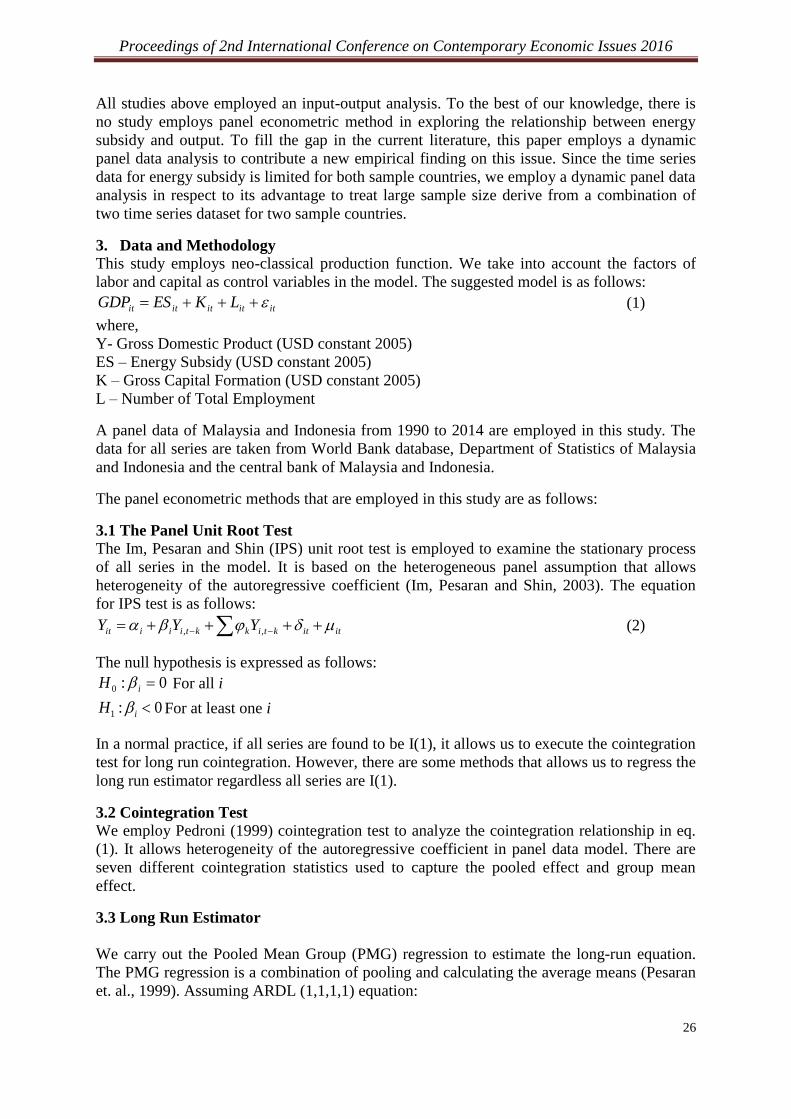
Proceedings of 2nd International Conference on Contemporary Economic Issues 2016
26
All studies above employed an input-output analysis. To the best of our knowledge, there is
no study employs panel econometric method in exploring the relationship between energy
subsidy and output. To fill the gap in the current literature, this paper employs a dynamic
panel data analysis to contribute a new empirical finding on this issue. Since the time series
data for energy subsidy is limited for both sample countries, we employ a dynamic panel data
analysis in respect to its advantage to treat large sample size derive from a combination of
two time series dataset for two sample countries.
3. Data and Methodology
This study employs neo-classical production function. We take into account the factors of
labor and capital as control variables in the model. The suggested model is as follows:
ititititit LKESGDP (1)
where,
Y- Gross Domestic Product (USD constant 2005)
ES – Energy Subsidy (USD constant 2005)
K – Gross Capital Formation (USD constant 2005)
L – Number of Total Employment
A panel data of Malaysia and Indonesia from 1990 to 2014 are employed in this study. The
data for all series are taken from World Bank database, Department of Statistics of Malaysia
and Indonesia and the central bank of Malaysia and Indonesia.
The panel econometric methods that are employed in this study are as follows:
3.1 The Panel Unit Root Test
The Im, Pesaran and Shin (IPS) unit root test is employed to examine the stationary process
of all series in the model. It is based on the heterogeneous panel assumption that allows
heterogeneity of the autoregressive coefficient (Im, Pesaran and Shin, 2003). The equation
for IPS test is as follows:
ititktikktiiiit YYY ,, (2)
The null hypothesis is expressed as follows:
0:0 iH For all i
1 : 0iH For at least one i
In a normal practice, if all series are found to be I(1), it allows us to execute the cointegration
test for long run cointegration. However, there are some methods that allows us to regress the
long run estimator regardless all series are I(1).
3.2 Cointegration Test
We employ Pedroni (1999) cointegration test to analyze the cointegration relationship in eq.
(1). It allows heterogeneity of the autoregressive coefficient in panel data model. There are
seven different cointegration statistics used to capture the pooled effect and group mean
effect.
3.3 Long Run Estimator
We carry out the Pooled Mean Group (PMG) regression to estimate the long-run equation.
The PMG regression is a combination of pooling and calculating the average means (Pesaran
et. al., 1999). Assuming ARDL (1,1,1,1) equation:
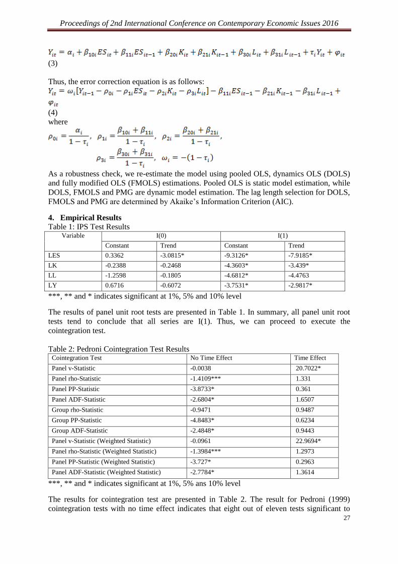
Proceedings of 2nd International Conference on Contemporary Economic Issues 2016
27
(3)
Thus, the error correction equation is as follows:
(4)
where
As a robustness check, we re-estimate the model using pooled OLS, dynamics OLS (DOLS)
and fully modified OLS (FMOLS) estimations. Pooled OLS is static model estimation, while
DOLS, FMOLS and PMG are dynamic model estimation. The lag length selection for DOLS,
FMOLS and PMG are determined by Akaike’s Information Criterion (AIC).
4. Empirical Results
Table 1: IPS Test Results Variable I(0) I(1)
Constant Trend Constant Trend
LES 0.3362 -3.0815* -9.3126* -7.9185*
LK -0.2388 -0.2468 -4.3603* -3.439*
LL -1.2598 -0.1805 -4.6812* -4.4763
LY 0.6716 -0.6072 -3.7531* -2.9817*
***, ** and * indicates significant at 1%, 5% and 10% level
The results of panel unit root tests are presented in Table 1. In summary, all panel unit root
tests tend to conclude that all series are I(1). Thus, we can proceed to execute the
cointegration test.
Table 2: Pedroni Cointegration Test Results Cointegration Test No Time Effect Time Effect
Panel v-Statistic -0.0038 20.7022*
Panel rho-Statistic -1.4109*** 1.331
Panel PP-Statistic -3.8733* 0.361
Panel ADF-Statistic -2.6804* 1.6507
Group rho-Statistic -0.9471 0.9487
Group PP-Statistic -4.8483* 0.6234
Group ADF-Statistic -2.4848* 0.9443
Panel v-Statistic (Weighted Statistic) -0.0961 22.9694*
Panel rho-Statistic (Weighted Statistic) -1.3984*** 1.2973
Panel PP-Statistic (Weighted Statistic) -3.727* 0.2963
Panel ADF-Statistic (Weighted Statistic) -2.7784* 1.3614
***, ** and * indicates significant at 1%, 5% ans 10% level
The results for cointegration test are presented in Table 2. The result for Pedroni (1999)
cointegration tests with no time effect indicates that eight out of eleven tests significant to

Proceedings of 2nd International Conference on Contemporary Economic Issues 2016
28
reject the null hypothesis. For the result of Pedroni (1999) cointegration tests with time effect,
two out of eleven tests significant to reject the null hypothesis. Thus, we can conclude that
our cointegration tests tend to support that all series are cointegrated in the long run.
Table 3: Long Run Estimator Variable Pooled OLS DOLS FMOLS PMG
ES 0.08175* 0.1151* 0.0981* 0.0897*
K 0.6778* 0.6022* 0.6412* 0.9326*
L -2.6239* -4.6808* -4.7661*** -1.8363*
***, ** and * indicates significant at 1%, 5% and 10% level
The result for long-run estimator is presented in Table 3. We use PMG estimator to interpret
the long-run coefficients. According to the ceteris paribus assumption, we can say that for
every 1% increase of ES leads to 0.09% increase on Y while other factors are constant. 1%
increases of K tend to increase 0.93% of Y while other factors are constant. 1% increases of
L leads to a decrease of Y about 1.83% while other factors are constant. All in all, ES has the
smallest magnitude change respect to a change of the exogenous variable of Y. In general,
our robustness checks (pooled OLS, DOLS and FMOLS) support our previous findings with
PMG estimation.
5. Conclusion and Policy Implication
In summary, this paper employs dynamic panel data analysis to explore the impact of energy
subsidy on economic production in Malaysia and Indonesia. Malaysia and Indonesia are oil
net exporter countries in ASEAN 5 while allocate a very high amount of energy subsidy in
their economy. We conclude that both countries are highly dependent on energy subsidy to
drive their economic growth. Our finding indicates that energy subsidy and capital have a
positive relationship with the output. Conversely, labor has a negative impact on output.
The finding that energy subsidy gives a positive impact on output is consistent with Jiang and
Lin (2014), Lin and Jiang (2011) and Plate (2014). The International Institute of Sustainable
Development (2012) reported that energy subsidy leads to the increase of income directly and
indirectly. Energy subsidy is directed to an increase of income when a private sector pays less
for energy; its consumer surplus is increased. On the other hand, energy subsidy is indirect
causes an increase of income when the price level is low from a cheaper energy cost that
reduces the cost of production. However, the cost of energy subsidy may transfer to the other
parties through the tax collection and deadweight loss. In the current development, Malaysia
and Indonesia are trying to rationalize their subsidy program subject to economic efficiency
improvement and to reduce their fiscal pressure. Octavian et al. (2005) and Rosli (2012)
suggested that the policymaker needs to introduce some effective offsetting policies to
cushion the adverse impact in respect to the absent of energy subsidy. Our empirical result
proved that the magnitude impact of energy subsidy is low compared to the other selected
factors.
Two types of policies with two different scenarios are recommended. First, the policymaker
could concentrate on offsetting policy if a reduction of subsidy is paramount for economic
sustainability. Optimizing an occupied labor as a wastage number of labor is expected to
increase energy wastage in the production as well. A part of that, a monetary regime needs to
be contemporary improved to accumulate enough capital to be invested in an economy to
support any progress of economic development. According to the fundamental of the neo-
classical production function, the energy input production is absorbed in both labor and
capital in the production to produce output (Alam, 2006). In a simple word, the more the
number of labor and capital are used in the production, the more the energy is consumed.

Proceedings of 2nd International Conference on Contemporary Economic Issues 2016
29
Second, if the policymaker would like to continue the energy subsidy program, we
recommend to rationalize the subsidy policy so that the subsidy becomes a productive tool to
improve economic development. International Institute of Sustainable Development (2013)
indicated that a direct energy subsidy distribution is not effective to increase the standard of
living of the targeted group. This is because a direct distribution of energy subsidy is enjoyed
much by the non-targeted group. The statistics show that 50% of high-income group enjoys
about 90% energy subsidy provided by the government in Indonesia (International Institute of
Sustainable Development, 2012). The same scenario was happened in Malaysia (The
International Institute of Sustainable Development, 2013). Hence, subsidy policy needs to be
rationalized to improve the energy subsidy distribution and become more effective to increase
the standard of living of a targeted group. Jiang and Lin (2014) suggested that selected
subsidy on energy resource or energy commodities should be removed based on its
magnitude impact in giving an adverse impact on an economy as a whole. The less the
magnitude impact of one subsidy of any energy resource or commodity, the more important it
is to be removed. The International Institute of Sustainable Development (2012) suggests the
policy maker should introduce an effective subsidy distribution which can exclude the non-
targeted group to excess to energy subsidy. Through that, it can be more effective to increase
the economic welfare as a whole as the targeted group will be benefited more.
Acknowledgement
We are thankful to the Ministry of Higher Education Malaysia for providing fund for this
study under RACE/e(2)/1249/2015(05). The second author would like to acknowledge
1001/PSOSIAL/AUPRM00536 from Universiti Sains Malaysia.
References
Alam, M. S., 2006. Economic Growth with Energy.MPRA Paper, No. 1260.
Arze Del Granado, J. Coady, D. and Gillingham, R., 2012. The unequal benefit of fuel
subsidies: are view of evidence for developing countries. World Development, 40(11),
p.2234-2248.
Im, K. S., Pesaran, M. H. and Shin, Y., 2003. Testing for Unit roots in heteroheneous panels.
Journal of Economic, 115, pp.53-74.
Isaak, D., 2015. Oil Security in ASIA and the Pacific. In Lee, M., Park, D. and Saunders, H.,
2015. Asia’s Energy Challenge: Key Issues and Policy Option, Routledge Taylor and
Francis Group, London and New York, pp.33-80.
Jiang, Z. and Lin, B., 2014. The perverse fossil fuel subsidies in china-the scale and effects.
Energy, 70, pp.411-419.
Jiang, Z. and Tan, J., 2013. How the removal of energy subsidy affects general price in china:
a study based on input-output model. Energy policy, 63(2013), pp.599-606.
Lin, B. and Jiang, Z., 2011. Estimates of energy subsidies in china and impact of energy
subsidy reform. Energy Economics, 33(2), pp.273-283.
Liu, W. and Li, H., 2011. Improving energy consumption structure: a comprehensive
assesment of fossil energy subsidies reform in china. Energy policy, 39(7), pp.4134-4143.
Manzoor, D., Shahmoradi, A. and Haqiqi, I., 2009. An analysis of energy price reform: A
CGE Approach. Mimeo, Imam Sadiq University and Ministry of Energy, Iran.
Octavian, R., Hakim, D. B., Sahara, H. and Siregar, S., 2005. The impact of Reducing Oil
Subsidy on Indonesian Macroeconomics Performance, Agrecultural Sector and Poverty
Incidences. MPIA Working Paper 2007-2008. Manila: Poverty and Econmic Policy (PEP)
Research Network.
Pedroni, P., 1999. Critical value for cointegration test in heteroheneous panels with multiple
regressors. Oxford Bulletin Statistics, 61, pp.653-670.

Proceedings of 2nd International Conference on Contemporary Economic Issues 2016
30
Pesaran, M. H., Shin, Y. and Smith, R. P., 1999. Pooled Mean Group Estimation of Dynamic
Heterogeneous Panels. Journal of the American Statistical Association, 94, pp.621-634.
Plate, M., 2014. The long-run macroeconomic impacts of fuel subsidies. Journal of
Development Economics, 107, pp.129-143.
Rosli, F., 2012. Malaysian Economy in 2012: Risks and Rewards? Institute of Strategic and
International Studies (ISIS) Malaysia, ISIS Praxis Seminar, No. 1/2012.
Solaymani, S. and Kari, F., 2014. Impacts of energy subsidy reform on the malaysian
economy and transportation sector. Energy Policy, 70 (2014), pp.115-125.
The International Institute for Sustainable Development, 2013. A Citizen’s Guide to Energy
Subsidies in Malaysia. Manitoba: International Institute for Sustainable Development.
The International Institute for Sustainable Development, 2012. A Citizen’s Guide to Energy
Subsidies in Indonesia. Manitoba: International Institute for Sustainable Development.
Van Beers, C., Van den Berch, J. C. J. M., 2011. Analysis perseverance of pervese subsidies
and their impact on trade and environment. Ecological Economics, 36(3), pp.475-486.

Proceedings of 2nd International Conference on Contemporary Economic Issues 2016
31
The relationship between Malaysia’s residential property price index and
residential properties loan supply
Chee-Hong Lawa,*
, Ghee-Thean Limb
a, b Economics program, School of Social Sciences, Universiti Sains Malaysia, Malaysia
aEmail: [email protected]
Abstract
This paper aims to examine the linkages between residential properties prices and residential
properties loans in Malaysia from 1999 to 2015, in addition to income level and the impact of
the economic crisis. Even though residential properties are a basic necessity, there is no
previous study that attempts to estimate the long-run and short-run relationship between loans
and price level in residential properties in Malaysia. It is believed that property price level
moves in the same direction as loan supply. The estimations are divided into two parts: the
detection of long run relationships and the estimation the long-run and short-run elasticities
from an ARDL model. The results support the hypothesis that the loan supply has a positive
impact on the residential price levels; the robustness test also supports this conclusion. This
implies the importance of closely monitoring the housing loan activities of banks to control
residential property prices.
Keywords: Residential properties price; residential property loan; Malaysia
1. Introduction
In recent decades, the increasing of housing prices in Malaysia attracted the attention of
researchers to investigate the determinants of housing prices. Among various types of
properties, residential properties are particularly important because housing is a basic need.
However, the residential price index of Malaysia increased almost two times from 1999 to
mid-2015. Concurrently, loans for residential properties also increased significantly. Many
researches have been conducted to determine the determinants of house prices in Malaysia
such as Ng (2006), Ahmad Faizal (2011), Dziauddin et al. (2013) and Tang and Tan (2015),
covering hedonic, bivariate and multivariate models. Besides, there are several papers test the
same issue using disaggregate data such as Ibrahim and Law (2014). These studies identify
several significant variables in their estimations. For instance, Ahmad Faizal (2011) and Tang
and Tan (2005) find cointegration relationships among house prices and interest rate. and the
Malaysia total and state-level house price index. Previous studies also tried to determine the
dynamic between housing prices with stock prices, covering national and state level data
(Lean, 2012; Lean and Smyth, 2014)
Nonetheless, to the best of my knowledge, only Ng (2006) and Ibrahim and Law (2014)
empirically analyse the impact of housing loans on the house price levels in Malaysia. Ng
(2006) focuses on investigating the determinants of the house prices using the Engle-Granger
estimation; he concludes that the long-run impact of loan supply on the properties prices is
positive. Nonetheless, his study has two weaknesses. First, the conclusion of cointegration
based on the unit roots test on the error terms in the Engle-Granger estimation are influenced
by dependent and independent variables; the impact is more obvious when more than two
variables are examined. Second, the Engle-Granger test involves two-step estimation. If the
error terms are erroneous in the first stage estimation, it will lead to a wrong conclusion. On
the other hand, the vector error correction model estimated by Ibrahim and Law (2014)
subject to the properties of the variables. In fact, they assume that a variable is differenced
stationary when there is a mixed conclusion from different unit root tests and exclude level
stationary variables. This paper attempts to fill the gap of knowledge by examining the
linkages between the residential price and residential loan. Additionally, the income level is
Proceedings of 2nd International Conference on Contemporary Economic Issues 2016
32
also examined. This paper applies an autoregressive distributed lag (ARDL) model to
illustrate the short-run and long-run relationships among the variables. The largest advantage
of the ARDL model is that we can determine the existence of long-run relationships among
variables without knowing the order of integration of the variables through Wald statistics.
The identification of order of integration is needed only when the Wald statistics fail to
confirm the variables are connected in the long-run (Narayan, 2004).
2. Data Descriptions
This paper includes two potential determinants of residential price levels, namely gross
domestic products (GDP) and loans for residential properties. This paper also includes
dummies that measure the impact of the subprime mortgage crisis in the US on Malaysia’s
residential market. According to Frankel and Saravelo (2012), the impact from the subprime
mortgage crisis was the most severe from the third quarter of 2008 to the first quarter of 2009.
Table 1 shows the indicator for each variable and the data sources. Quarterly data from the
first quarter of 1999 to the second quarter of 2015 are tested. All variables are seasonally
adjusted using the Census X-13 technique and are transformed into natural logarithm form.
Table 1: Variables Indicators and Data Sources Variables Indicators Data Sources
Residential properties prices Residential properties prices index
(base year=2010)
Bank for International Settlements
Loans for residential properties
prices
The loans disbursed for residential
properties
Monthly Statistical Bulletin, Bank
Negara Malaysia
Income level Gross domestic products (current
price)
Monthly Statistical Bulletin, Bank
Negara Malaysia
In particular, the residential properties prices cover all types of new and existing dwellings in
Malaysia. The loan for residential properties, on the other hand, refers to the loans for
residential properties from the Malaysian banking system. Gross domestic product (GDP) is a
common indicator of income level of a country in many previous studies. All estimations are
conducted using Eviews 9.
3. Methodology and Model Specification
Due to relatively small sample size and to preserve the degree of freedom, this paper limits
the examined variables into two potential determinants of housing prices, namely housing
loan and output level. The first estimation is to determine the existence of cointegration
among the variables by constructing an unrestricted error correction model that can be
illustrated by equation (1).
(1)
where denotes the first differenced of variables, 0 is the constant, LRP is the natural
logarithm of residential price index, LGDP is the natural logarithm of GDP, LLOAN is the
natural logarithm of residential loans and CRISIS are the dummies representing the subprime
mortgage crisis. The lag length is decided using the Hendry general to specific method. In
order to test the existence of long-run relationship, F-statistic or Wald test is applied to test
the null hypothesis of 0321 against the alternative hypothesis of 0321 .
The failure to reject the null hypothesis means there are no long-run relationships among the
variables in the model. However, the F-statistics do not have standard distribution and
therefore this study applies the critical values of F-statistic generated by Narayan (2005) that
are appropriate when the number of observations in a study range from 30 to 80. There are

Proceedings of 2nd International Conference on Contemporary Economic Issues 2016
33
two bounds of critical values: the upper bound where all variables are I(1) and the lower
bound where all variables are I(0). There is evidence that the variables have long-run
relationships if the F-statistic value is higher than the critical values. The opposite conclusion
is arrived if the F-statistic value is below the critical value. Nonetheless, the outputs are
inconclusive when the F-statistic value falls between the bounds. As mentioned in the
introduction, we can skip the unit root tests if there are long-run relationships among the
variables.
If the cointegrated relationship is confirmed, the next step is to construct a long-run
relationship from an ARDL (p, p1, p2) model, as showed below:
(2)
The model is estimated using OLS estimation procedure and the number of lag in equation (2)
is determined by Akaike information criterion (AIC); the model with the lowest AIC will be
selected. There are two important outputs from the ARDL equation: long-run and short-run
elasticities. The long-run equation has the following general form.
(3)
We apply the following formulae to measure the long-run elasticity of residential properties
loan ( 1 ), GDP ( 2 ) and crisis ( 3 ), respectively.
On the other hand, the short-run equations can be illustrated as below:
(4)
where 1t is the error correction terms (ECT) and are derived from equation (2). Its
coefficient represents the speed-of-adjustment. Hendry general to specific method is applied
to determine the appropriate lag length. The error terms should be statistically significant and
have a negative sign; this is important because it means any deviation from the long-run
equilibrium in the short term will be eliminated. The following diagnostic tests are conducted
to ensure the fitness of the model: Jarque-Bera normality test, Breusch-Godfrey serial
correlation LM test and Breusch-Pagan-Godfrey serial heteroskedasticity test. In addition, the
stability of the error correction model is also tested by observing the roots of the equation.
Eviews 9 is applied for all estimations in this paper.

Proceedings of 2nd International Conference on Contemporary Economic Issues 2016
34
4. Results Discussion
The results discussion begins with the construction of unrestricted error correction model.
Table 2 illustrates the F-statistics and the relevant critical values at 1%, 5% and 10%
significance levels. The result indicates that the null hypothesis is rejected at the 5%
significance level. Hence, there is cointegration in the model. Following this, an ARDL (p, p1
and p2) model is constructed and the optimal lag length is decided by using the AIC. Figure 1
shows that the optimal model of ARDL model is found when the ARDL (4,0,4) that has four
lags is included for LRP and LLOAN. Table 3 contains the estimation outputs of the ARDL
(4,0,4) model.
Table 2: F-statistic Output
F-statistic 4.4015
Critical Value
1% I(0)= 4.068 I(1)=5.250
5% I(0)= 2.962 I(1)=3.910
10% I(0)= 2.496 I(1)=3.346
Note: Restricted intercept and no trend (k=3, n=60), available from Narayan (2005)
-6.56
-6.52
-6.48
-6.44
-6.40
-6.36
ARDL(4
, 0, 4)
ARDL(4
, 1, 4)
ARDL(4
, 2, 4)
ARDL(3
, 0, 4)
ARDL(1
, 0, 4)
ARDL(
4, 3, 4)
ARDL(3
, 1, 4)
ARDL(1
, 1, 4)
ARDL(2
, 0, 4)
ARDL(4
, 4, 4)
ARDL(3
, 2, 4)
ARDL(1
, 2, 4)
ARDL(2
, 1, 4)
ARDL(3
, 3, 4)
ARDL(1
, 3, 4)
ARDL(2
, 2, 4)
ARDL(3
, 4, 4)
ARDL(1
, 4, 4)
ARDL(2
, 3, 4)
ARDL(3
, 0, 0)
Akaike Information Criteria (top 20 models)
Figure 1 : The top 20 models based on AIC
From the outputs in Table 3, the long-run elasticities of the independent variables are
generated and presented in the Table 4. The results show that only the residential properties
loans and the global financial crisis have statistically significant impact on the residential
price at the 1% and 10% significance level, respectively. In particular, one percent increases
in the residential properties loan rises the residential price by 0.99%. On the other hand, the
global financial negatively affects the residential price by decreasing it by 0.42%. Particularly,
an increase in the loan supply could raise the ability to own a property through bank
borrowing, which subsequently pushes up the residential price level if the house supply is
inelastic. This is also in accordance to the demand-pull inflation contributed by credit supply.
The occurrence of economic crisis is expected to arouse negative sentiment among the
properties buyers and investors. This inevitably reduces their appetite for the properties,
including residential dwellings, which is in accordance with the risk aversion hypothesis.
Finally, the error correction terms (ECT) term indicates the adjustment of deviation back to
long-run relationship is small (3.9%).
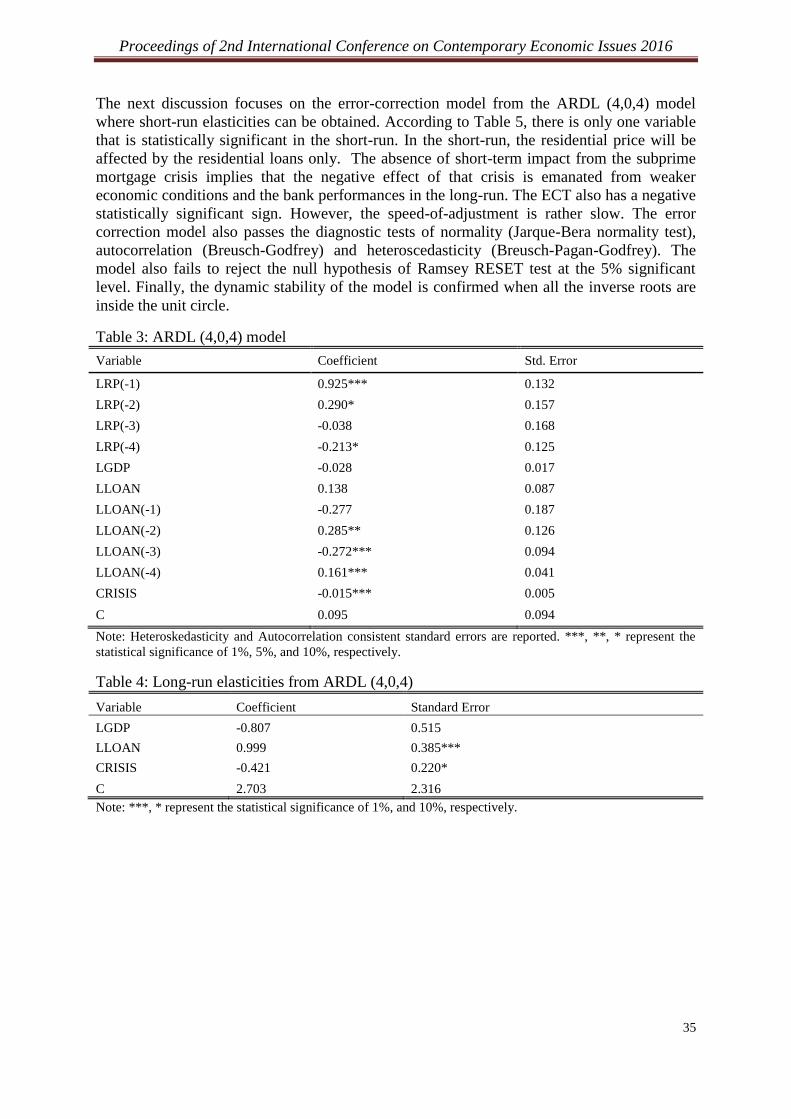
Proceedings of 2nd International Conference on Contemporary Economic Issues 2016
35
The next discussion focuses on the error-correction model from the ARDL (4,0,4) model
where short-run elasticities can be obtained. According to Table 5, there is only one variable
that is statistically significant in the short-run. In the short-run, the residential price will be
affected by the residential loans only. The absence of short-term impact from the subprime
mortgage crisis implies that the negative effect of that crisis is emanated from weaker
economic conditions and the bank performances in the long-run. The ECT also has a negative
statistically significant sign. However, the speed-of-adjustment is rather slow. The error
correction model also passes the diagnostic tests of normality (Jarque-Bera normality test),
autocorrelation (Breusch-Godfrey) and heteroscedasticity (Breusch-Pagan-Godfrey). The
model also fails to reject the null hypothesis of Ramsey RESET test at the 5% significant
level. Finally, the dynamic stability of the model is confirmed when all the inverse roots are
inside the unit circle.
Table 3: ARDL (4,0,4) model
Variable Coefficient Std. Error
LRP(-1) 0.925*** 0.132
LRP(-2) 0.290* 0.157
LRP(-3) -0.038 0.168
LRP(-4) -0.213* 0.125
LGDP -0.028 0.017
LLOAN 0.138 0.087
LLOAN(-1) -0.277 0.187
LLOAN(-2) 0.285** 0.126
LLOAN(-3) -0.272*** 0.094
LLOAN(-4) 0.161*** 0.041
CRISIS -0.015*** 0.005
C 0.095 0.094
Note: Heteroskedasticity and Autocorrelation consistent standard errors are reported. ***, **, * represent the
statistical significance of 1%, 5%, and 10%, respectively.
Table 4: Long-run elasticities from ARDL (4,0,4)
Variable Coefficient Standard Error
LGDP -0.807 0.515
LLOAN 0.999 0.385***
CRISIS -0.421 0.220*
C 2.703 2.316
Note: ***, * represent the statistical significance of 1%, and 10%, respectively.
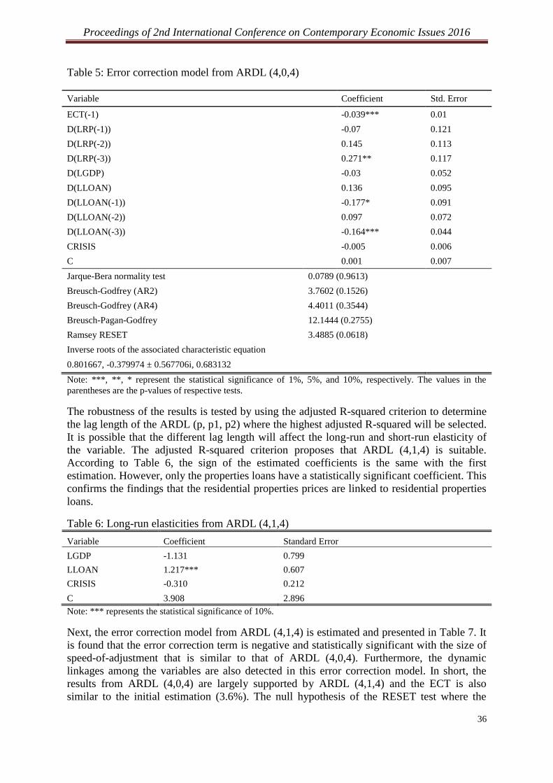
Proceedings of 2nd International Conference on Contemporary Economic Issues 2016
36
Table 5: Error correction model from ARDL (4,0,4)
Variable Coefficient Std. Error
ECT(-1) -0.039*** 0.01
D(LRP(-1)) -0.07 0.121
D(LRP(-2)) 0.145 0.113
D(LRP(-3)) 0.271** 0.117
D(LGDP) -0.03 0.052
D(LLOAN) 0.136 0.095
D(LLOAN(-1)) -0.177* 0.091
D(LLOAN(-2)) 0.097 0.072
D(LLOAN(-3)) -0.164*** 0.044
CRISIS -0.005 0.006
C 0.001 0.007
Jarque-Bera normality test 0.0789 (0.9613)
Breusch-Godfrey (AR2) 3.7602 (0.1526)
Breusch-Godfrey (AR4) 4.4011 (0.3544)
Breusch-Pagan-Godfrey 12.1444 (0.2755)
Ramsey RESET 3.4885 (0.0618)
Inverse roots of the associated characteristic equation
0.801667, -0.379974 ± 0.567706i, 0.683132
Note: ***, **, * represent the statistical significance of 1%, 5%, and 10%, respectively. The values in the
parentheses are the p-values of respective tests.
The robustness of the results is tested by using the adjusted R-squared criterion to determine
the lag length of the ARDL (p, p1, p2) where the highest adjusted R-squared will be selected.
It is possible that the different lag length will affect the long-run and short-run elasticity of
the variable. The adjusted R-squared criterion proposes that ARDL (4,1,4) is suitable.
According to Table 6, the sign of the estimated coefficients is the same with the first
estimation. However, only the properties loans have a statistically significant coefficient. This
confirms the findings that the residential properties prices are linked to residential properties
loans.
Table 6: Long-run elasticities from ARDL (4,1,4)
Variable Coefficient Standard Error
LGDP -1.131 0.799
LLOAN 1.217*** 0.607
CRISIS -0.310 0.212
C 3.908 2.896
Note: *** represents the statistical significance of 10%.
Next, the error correction model from ARDL (4,1,4) is estimated and presented in Table 7. It
is found that the error correction term is negative and statistically significant with the size of
speed-of-adjustment that is similar to that of ARDL (4,0,4). Furthermore, the dynamic
linkages among the variables are also detected in this error correction model. In short, the
results from ARDL (4,0,4) are largely supported by ARDL (4,1,4) and the ECT is also
similar to the initial estimation (3.6%). The null hypothesis of the RESET test where the
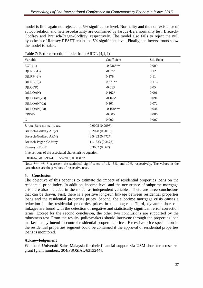
Proceedings of 2nd International Conference on Contemporary Economic Issues 2016
37
model is fit is again not rejected at 5% significance level. Normality and the non-existence of
autocorrelation and heteroscedasticity are confirmed by Jarque-Bera normality test, Breusch-
Godfrey and Breusch-Pagan-Godfrey, respectively. The model also fails to reject the null
hypothesis of Ramsey RESET test at the 5% significant level. Finally, the inverse roots show
the model is stable.
Table 7: Error correction model from ARDL (4,1,4)
Variable Coefficient Std. Error
ECT (-1) -0.036*** 0.009
D(LRP(-1)) -0.072 0.12
D(LRP(-2)) 0.179 0.11
D(LRP(-3)) 0.271** 0.116
D(LGDP) -0.013 0.05
D(LLOAN) 0.162* 0.096
D(LLOAN(-1)) -0.165* 0.091
D(LLOAN(-2)) 0.101 0.072
D(LLOAN(-3)) -0.168*** 0.044
CRISIS -0.005 0.006
C 0.002 0.007
Jarque-Bera normality test 0.0005 (0.9998)
Breusch-Godfrey AR(2) 3.2028 (0.2016)
Breusch-Godfrey AR(4) 3.5432 (0.4727)
Breusch-Pagan-Godfrey 11.1333 (0.3472)
Ramsey RESET 3.3632 (0.067)
Inverse roots of the associated characteristic equation
0.801667, -0.379974 ± 0.567706i, 0.683132
Note: ***, **, * represent the statistical significance of 1%, 5%, and 10%, respectively. The values in the
parentheses are the p-values of respective tests.
5. Conclusion
The objective of this paper is to estimate the impact of residential properties loans on the
residential price index. In addition, income level and the occurrence of subprime mortgage
crisis are also included in the model as independent variables. There are three conclusions
that can be drawn. First, there is a positive long-run linkage between residential properties
loans and the residential properties prices. Second, the subprime mortgage crisis causes a
reduction in the residential properties prices in the long-run. Third, dynamic short-run
linkages are found with the detection of negative and statistically significant error correction
terms. Except for the second conclusion, the other two conclusions are supported by the
robustness test. From the results, policymakers should intervene through the properties loan
market if they intend to control residential properties prices. Excessive price speculation in
the residential properties segment could be contained if the approval of residential properties
loans is monitored.
Acknowledgement
We thank Universiti Sains Malaysia for their financial support via USM short-term research
grant [grant numbers: 304/PSOSIAL/6313244].
Proceedings of 2nd International Conference on Contemporary Economic Issues 2016
38
References
Ahmad Faizal, A.Z., 2011. Causality of residential properties price movement in Malaysia.
Available at: < https://mpra.ub.uni-muenchen.de/47682/3/> [Accessed 25 May 2016].
Dziauddin, M.F., Alvanides, S. and Powe, N., 2013. Estimating the Effects of Light Rail
Transit (LRT) System on the Property. Jurnal Teknologi, 61, pp.35–47.
Frankel, J. and Saravelos, G., 2012. Can leading indicators access country vulnerability?
Evidence from the 2008-2009 global financial crisis. Journal of International Economics,
87, pp.216-231.
Ibrahim, M.H. and Law, S.H., 2014. House prices and bank credits in Malaysia: An aggregate
and disaggregate analysis. Habitat International, 42, pp.111–120.
Lean, H.H., 2012. Wealth effect or credit-price effect? Evidence from Malaysia. Procedia
Economics and Finance, 1, pp.259-268.
Lean, H.H. and Smyth R., 2014. Dynamic interaction between house prices and stock prices
in Malaysia. International Journal of Strategic Property Management, 18, pp.163-177.
Narayan, K.P., 2004. Reformulating critical values for bound F-statistics approach to
cointegration: An application to the tourism demand model for Fiji. Monash University
Department of Economics Discussion Papers no. 02/04. Melbourne: Department of
Economics.
Narayan, K.P., 2005. The saving and investment nexus for China: evidence from
cointegration tests. Applied Economics, 37, pp.1979-1990.
Ng, A., 2006. Housing and mortgage market in Malaysia. In B. Kusmiarso, ed. 2006.
Housing and mortgage markets in the SEACEN countries. Kuala Lumpur: SEACEN
centre. pp. 128-129
Tang, T.C. and Tan, P.P., 2015. Real interest rate and house prices in Malaysia: An empirical
study. Economics Bulletin, 35, pp.270-275.
Proceedings of 2nd International Conference on Contemporary Economic Issues 2016
39
The Prevalence of Overemployment in Penang: A Preliminary Analysis
Jacqueline Liza Fernandeza,*
and Ee Shiang Limb
a,b School of Social Sciences, Universiti Sains Malaysia, Malaysia
aEmail : [email protected]
bEmail : [email protected]
Abstract
Nowadays, workers tend to face the problem of overemployment where desired working
hours are less than their actual working hours. Some overemployed workers desire to work
less hours although there may be a concomitant decline in earnings. This research is
conducted to study the factors that are related to the employment status of workers in Penang
with regard to being overemployed or otherwise. This research uses primary data that was
collected in a survey that was done in one particular state in Malaysia, namely Penang. The
questionnaires were distributed to workers in different areas in Penang. A total of 525
respondents were surveyed in this study. This paper reports the preliminary findings of the
study by presenting the bivariate relationship between the employment status of workers and
various demographic, socio-economic and work-related variables. The initial findings of this
study provide the basis for some general conclusions and policy implications on the issue of
overemployment in Penang.
Keywords: Overemployment; hours mismatch; actual hours of work; preferred hours of
work.
1. Introduction
One important aspect of working conditions is working time. In industrialised countries, 22
percent of the workforce surveyed worked more than 48 hours a week, which the
International Labour Organisation defines as excessive (Lee, McCann and Messenger, 2007).
In Malaysia, the Malaysian Employment Act defines the standard work week as 48 hours,
with a maximum of 8 working hours per day and 6 working days per week. However, in a
survey that was done by an online recruitment firm involving 954 employees across various
industries in Malaysia, it was revealed that 70 percent of the workers worked 2-5 extra hours
daily due to unreasonable deadlines and work overload. It was also reported that 63 percent
of workers felt that they were not spending enough time with their families due to long
working hours (JobStreet, 2013).
Although there are statutory regulations on working time in most countries, the problem of
hour mismatches still persists. Hour mismatches arise when workers actual hours of work
differ from their desired or preferred hours of work. There are two types of hour mismatches;
the first is overemployment which occurs when actual hours of work exceeds desired hours of
work and the second is underemployment which occurs when actual hours of work falls short
of desired hours of work. The focus of this paper is overemployment. The issue of
overemployment merits attention because of its negative consequences on work-life balance,
workers well-being and their job performance. The main objective of this paper is to identify
empirically the factors associated with overemployment.
* Corresponding author

Proceedings of 2nd International Conference on Contemporary Economic Issues 2016
40
2. Literature Review
Overemployment is often related to demographic, socio-economic and work-related factors.
The first group of factors is demographic variables which include age and gender; the second
set of factors is socio-economic factors which encompasses income, presence of full-time
homemaker and childcare responsibilities. The last category of factors is work-related factors
such as hours of work, job satisfaction and occupation.
Most studies take into account the relationship between overemployment and two key
demographic variables, which are age and gender. Age may influence desired work hours as
younger workers who are just entering the workforce are likely to have very different work
preferences than those who are older and nearing retirement. Previous studies (e.g. Golden
and Gebreselassie, 2007; Angrave and Charlwood, 2015) show a clear pattern by age, with
overemployment low among young workers but rising with age. Another demographic
variable that is of interest is gender. Women tend to do a greater share of household work
than men; in addition, gender inequalities in the work place tend to reduce women’s job
commitment and tendency to make labour market work their central priority (Reynolds,
2005). As a result, women tend to desire fewer hours of work. Empirical evidence (e.g.
Sousa-Poza and Henneberger’s (2002) study which covers twenty one countries; Golden and
Gebreselassie’s (2007) research in the United States) indicates that women are more likely to
be overemployed than men.
The second group of factors that is linked to overemployment is socio-economic factors. One
of these factors is income. Theoretically, an increase in wage income induces an increase in
the allocation of time for leisure (due to the income effect), thus decreasing the likelihood of
overemployment. On the other hand, an increase in wages increases the opportunity cost of
leisure; therefore a higher wage may encourage workers to sacrifice leisure for wages/work
(due to the substitution effect), thus increasing the likelihood of overemployment. The net
effect of an increase in wage income on overemployment is theoretically indeterminate. In
the United States, employees who have higher wage incomes do more work than their lower
paid peers but they do not have a stronger passion for work (Reynolds and Aletraris, 2007). It
is argued that higher paid employees seem to be working more hours reluctantly because
employers have packaged their high incomes with long workweeks (Clarkberg and Moen,
2001).
The other socio-economic variables are family characteristics such as the presence of a full-
time homemaker and childcare duties. All workers have to allocate time for labour market
work and their personal life. The time squeeze may be more pronounced in the absence of a
full-time homemaker (e.g. in the case of single working parents and dual-earner couples with
children) and this can give rise to an unmet desire for fewer working hours (Jacobs and
Gerson, 2001). In contrast, breadwinners (particularly men) can work many hours because
they have spouses who perform unpaid domestic work (Reynolds, 2014). Furthermore, these
men may feel responsible for the economic well-being of their families (Kaufman &
Uhlenberg 2000), and this would increase their desire for additional work hours and reduce
the likelihood of overemployment. Another important family characteristic is childcare duties,
which is proxied by number of children in the household and age of the youngest child. The
difficulty of integrating paid work and childcare increases the probability of individuals
wanting less working hours in order to spend more time with their children. This occurs
among women workers (Van der Lippe, 2001) as well as men workers (Abendroth, Pausch
and Bohm, 2014).
Proceedings of 2nd International Conference on Contemporary Economic Issues 2016
41
The last category of factors is work-related factors such as hours of work, job satisfaction and
occupation. The link between hours of work and overemployment can be understood in the
context of the work-leisure model of time allocation. The hour mismatch problem arises
when an individual has not attained his/her optimum position. Workers who spend many
hours at work often want to reduce their working hours. According to Sousa-Poza and
Henneberger (2002), the percentage of workers who desire fewer hours of work rises as
working hours increase. Empirical studies show that overemployment is significantly related
to hours of work (Reynolds, 2003; 2004; 2005). Golden and Gebreselassie’s (2007) study
shows that full-time workers have a progressively higher probability of being overemployed
corresponding to the length of their usual weekly hours, relative to those working 35-39
hours. Another work-related variable is job satisfaction. Satisfaction with paid labour is
expected to decrease the likelihood that individuals encounter hour mismatches. The negative
impact of job satisfaction on hour mismatches is documented in the literature (e.g. Bloch and
Taylor, 2012; Reynolds and Aletraris, 2007). The last factor is type of occupation. Some jobs
require more working hours. Golden and Gebreselassie (2007) opine that overemployment is
more likely to occur in occupations for which there are no legally required overtime pay
premia for increasing hours as well as occupations that tend to be paid by salary rather than
hourly wages. These job characteristics are more common among white-collar workers.
According to Reynolds (2003), professionals are more likely to desire fewer hours of work in
comparison to blue-collar workers. Golden’s (2004) study also found that white-collar
workers in managerial and professional groups have significantly higher levels of
overemployment while blue-collar workers are less likely to experience overemployment.
3. Data and Methodology
Primary data is used in this study. The survey data was collected using a structured
questionnaire that was distributed to workers in Penang, a northern state in Malaysia. A total
of 525 respondents were surveyed comprising 207 (39.4 percent) Malays, 239 (45.5 percent)
Chinese and 79 (15 percent) Indians and others. This is similar to the ethnic composition of
Penang’s population which is 40.9 percent Malays, 41.5 percent Chinese and 17.6 percent
Indian and others. The sample comprises 253 (48.2 percent) males and 272 (51.8 percent)
females which also reflects the state’s gender composition of 50.01 percent males and 49.99
percent females.
An analysis of overemployment in Penang is presented in the next section based on cross
tabulations in order to examine the association between overemployment and demographic,
socio-economic and work-related variables. The Chi-square statistic is used to examine
whether the relationship between overemployment and the variable in question is significant
or not. The employment status of workers is divided into two categories that is overemployed
and not overemployed. In this study, overemployed workers refer to individuals who desire to
work fewer hours for less pay. Workers who are not overemployed are those who either
prefer to maintain current working hours for the same pay or prefer to work more hours for
more pay.

Proceedings of 2nd International Conference on Contemporary Economic Issues 2016
42
4. Empirical Results
The sample in this study consists of 525 workers, of which 114 individuals (21.71 percent)
are overemployed and the remaining 411 individuals (78.29 percent) are not overemployed.
Table 1 provides a snap shot of the employment status of respondents who are categorised
into different groups based on selected demographic, socio-economic and work-related
factors, and the chi-square statistics.
The sample of 525 workers used in this study comprises 253 males (48.2 percent) and 272
females (51.8 percent). Among the 114 workers who are overemployed, 51 (44.7 percent) are
males and 63 (55.3 percent) are females. Table 1 shows that the incidence of
overemployment is slightly higher for women than for men, that is 23.2 percent of women
and 20.2 percent of men prefer fewer working hours. However, the Chi-square test shows that
gender is not significantly related to overemployment. This may be due to the influence of
countervailing forces of other factors (which are linked to overemployment and gender) that
are not held constant in this tabular analysis, which obliterates the relationship between the
two variables.
The majority of the respondents (70 percent) are relatively young workers, below the age of
35. By comparing the percentage of workers who are overemployed in each age group, it can
be seen that the incidence of overemployment tends to increase with age; less than 20 percent
of workers below the age of 30 are overemployed; the corresponding figure is between 20 –
30 percent in the 31 – 50 age bracket and it is greater than 40 percent for older workers above
the age of 50. This result is similar to the findings of previous studies (Golden and
Gebreselassie, 2007; Angrave and Charlwood, 2015) which show that the incidence of
overemployment is positively related with age. It is speculated that the higher prevalence of
overemployment (the desire to work fewer hours for less pay) among older workers may be
due to health reasons, greater financial stability and the preference for flexible working
options prior to retirement.
Next, we turn to the socio-economic variables which include income and family
characteristics. There is a positive relationship between income and the incidence of
overemployment. The incidence of overemployment is positively related to the level of wage
income; it is lowest (18.9 percent) in the low wage income group and highest (40 percent) in
the high wage income group. The positive relationship between income and overemployment
suggests that as income rises, there is an increase the percentage of workers who desire fewer
hours of work and are willing to forgo some portion of their earnings for reduced hours of
work. This implies that higher income affords workers this choice since they are well off
economically and have strong financial footing as argued by Reynolds (2003).
Family characteristics include factors such as presence of full-time homemaker (proxied by
spouse’s working status) and childcare responsibilities. There are 175 dual earner families
without a full-time homemaker (166 respondents with spouses who are working full-time and
9 with spouses working part-time). There are 350 respondents who are either single or with
spouses who are not employed. The data shows that slightly over 30 percent of respondents
with a working spouse desire fewer hours of work. In the case of those with a non-working
spouse or are single, only 17.1 percent are overemployed. In short, the incidence of
overemployment is greater for those who have a working spouse; this is possibly because of
the time squeeze that both partners encounter in dividing their time for labour market work
and household duties.
Childcare responsibilities are reflected by the number of children and age of youngest child.
The incidence of overemployment varies by the number of children in the household. Table 1
shows that 44 percent of respondents with 4 children or more are overemployed; the

Proceedings of 2nd International Conference on Contemporary Economic Issues 2016
43
corresponding figure is about 30 percent for those with 2 or 3 children, 23 percent for those
with 1 child and only 16.4 percent for those with no children. This shows that the incidence
of overemployment increases as the number of children increases. The incidence of
overemployment also varies by the age of the youngest child in the household. The data
shows that 50 percent of workers with youngest child more than 17 years old desire to reduce
their working hours; the corresponding figure is between 23-26 percent for workers whose
youngest child is below 17 years and it is 16.5 percent for those with no children. The results
suggest that overemployment is highest for workers with older children (above 17 years) in
comparison to those with younger children. There are at least two possible reasons why
workers whose youngest child is above 17 years old are overemployed. Firstly, these workers
are likely to be in the older age group and more likely to face overemployment given that the
desire for few hours is positively related to age. Secondly, workers whose youngest child is
above 17 years old probably have older children who are working and providing financial
support to the family and this gives these workers the option to reduce hours of work and
earn a lesser salary. But the incidence of overemployment does not vary greatly for those
with pre-school children (below 6 years), primary level children (6-12 years) and secondary
level children (13-17 years). This may be because workers with pre-school or school-age
children can rely on unpaid / paid caregivers to provide childcare and so the desire for fewer
hours of work is not markedly different for those with children in these age groups.
In this study, almost 70 percent of workers work less than 48 hours per week, while 23
percent work more than 48 hours per week and 7.8 percent work exactly 48 hours per week.
The high proportion of workers working less than 48 hours per week could probably be
because there are a number of organisations that operate five days per week. The incidence of
overemployment tends to increase with working hours. The incidence of overemployment is
highest among workers working more than 48 working hours (31.7 percent), followed by
those working exactly 48 hours per week (26.8 percent) and lowest for those working less
than 48 hours per week (17.9 percent). The low incidence of overemployment among
workers with less than 48 hours per week is not surprising since this group would include
part-time workers who work short hours. The result of the chi square test indicates that the
relationship between working hours and employment status is significant at 1%.
Workers’ job satisfaction is measured by a 5-point Likert scale ranging from 1 (lowest job
satisfaction) to 5 (highest job satisfaction). Job satisfaction of workers is classified as low if
the score is 1 or 2, medium if the score is 3 and high if the score is 4 or 5. Among the 525
respondents, more than three-fifths of them have high job satisfaction, and followed by 27.6
percent with medium job satisfaction and 9.1 percent with low job satisfaction.
Overemployment appears to be inversely related to the level of job satisfaction. The
incidence of overemployment among workers with high job satisfaction (19.6 percent) is
lower than those with medium job satisfaction (23.4 percent). Similarly, the incidence of
overemployment for workers with medium job satisfaction is lower than those with low job
satisfaction (31.2 percent). Workers with low job satisfaction tend to have the greatest desire
to reduce their working hours. Nevertheless, the result of the chi square test indicates that
there is no significant relationship between employment status and job satisfaction at 1 %
level.
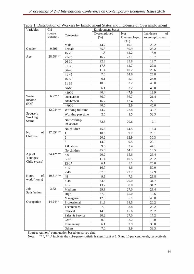
Proceedings of 2nd International Conference on Contemporary Economic Issues 2016
44
Table 1: Distribution of Workers by Employment Status and Incidence of Overemployment Variables Chi-
square
statistics Categories
Employment Status
Overemployed
(%)
Not
Overemployed
(% )
Incidence of
overemployment
Gender
0.696
Male 44.7 49.1 20.2
Female 55.3 50.9 23.2
Age
28.68*** 15-20 1.8 12.2 3.9
21-25 16.7 23.1 16.7
26-30 22.8 25.8 19.7
31-35 17.5 12.7 27.8
36-40 11.4 10.2 23.6
41-45 7.0 54.6 25.8
46-50 6.1 5.1 25.0
51-55 10.5 3.2 48.0
56-60 6.1 2.2 43.8
Wage
Income
(RM)
6.27** <2000 40.4 47.9 18.9
2001-4000 36.0 36.7 21.4
4001-7000 16.7 12.4 27.1
>7000 40.0 2.9 40.0
Spouse’s
Working
Status
12.94*** Working full time 44.7 22.8 30.7
Working part time 2.6 1.5 33.3
Not working/
no spouse 52.6 70.6 17.1
No of
Children
17.65*** No children 45.6 64.5 16.4
1 10.5 9.7 23.1
2 20.2 12.9 30.3
3 14.0 9.5 29.1
4 & above 9.6 3.4 44.1
Age of
Youngest
Child (years)
24.42*** No children 45.6 64.2 16.5
< 6 20.2 15.6 26.4
6-12 11.4 10.5 23.2
13-17 6.1 5.1 25.0
> 17 16.7 4.6 50.0
Hours of
work (hours)
10.81*** < 48 57.0 72.7 17.9
48 9.6 7.3 26.8
> 48 33.3 20.0 31.7
Job
Satisfaction
3.72 Low 13.2 8.0 31.2
Medium 29.8 27.0 23.4
High 57.0 65.0 19.6
Occupation
14.24** Managerial 12.3 5.1 40.0
Professional 31.6 34.5 20.2
Technicians 7.9 8.8 20.2
Clerical 14.0 15.6 20.2
Sales & Service 20.2 27.0 17.2
Craft 0.9 2.2 10.0
Elementary 6.1 2.9 36.8
Others 7.0 3.9 33.3
Source: Authors’ computation based on survey data.
Note: ***, ** ,* indicate the chi-square statistic is significant at 1, 5 and 10 per cent levels, respectively.

Proceedings of 2nd International Conference on Contemporary Economic Issues 2016
45
This study uses the Department of Statistics’ classification of occupations. The sample
comprises 35 managerial workers (6.7 percent), 178 professional workers (33.9 percent), 45
technicians (8.6 percent), 80 clerical workers (15.2 percent), 134 sales and service workers
(25.5 percent), 10 craft/related trade workers (1.9 percent), 19 elementary workers (3.6
percent), and 24 in other occupations (4.6 percent). The highest incidence of overemployment
is among managerial workers (40 percent). The high incidence of overemployment in the
managerial group is noted in other studies e.g. Golden (2004), Golden and Gebreselassie
(2007). Another group with a high incidence of overemployment is elementary workers (36.8
percent). The chi square test shows that the relationship between occupations and
employment status is significant at 5%.
5. Conclusions and Policy Implications
The incidence of overemployment tends to be higher for the following groups: older workers,
high-income workers, individuals with a working spouse, more children and older children,
workers who clock in more than 48 hours as well as managerial and elementary workers.
The above findings are used to discuss tentative policy implications. The high incidence of
overemployment among older workers suggests a need to offer them part-time jobs or job-
sharing options. This will enable firms to retain senior and experienced employees. Another
key finding is the positive relationship between overemployment and number of children.
This implies the need for family-friendly policies (e.g. parental leave) to reduce
overemployment. Providing childcare facilities in or near the workplace is another possible
solution.
The results show that overemployment is prevalent among workers who work more than 48
hours per week. The move to reconfigure working time policies and limit overtime work is a
step in the right direction to reduce overemployment. The five dimensions of decent working
time propagated by ILO - healthy working time, “family-friendly” working time, gender
equality through working time, productive working time and choice and influence regarding
working time – provide a framework for policies which can advance the goal of decent
working time. The prevalence of overemployment also increases with earnings. It is
suggested that high income workers be given the option of working remotely (if the nature of
their work permits it) in order to reduce overemployment. Finally, there is a prevalence of
overemployment among managerial and elementary workers. Mitigating overemployment in
the latter group is seen as a matter of greater urgency because this group is relatively more
vulnerable. Labour laws should ensure that these workers are not subject to exploitation in
terms of their hours of work.
Acknowledgement
This research is funded by the Short Term Grant (No: 304/PSOSIAL/6313119) provided by
Universiti Sains Malaysia, Penang.
References
Abendroth, A.J., Pausch, S. and Bohm, S., 2014. German Fathers and Their Preference to
Reduce Working Hours to Care for Their Children. SFB 882 Working Paper Series. Vol
41. Bielefeld: DFG Research Center (SFB) 882 from Heterogeneities to Inequalities
Angrave D and Charlwood A., 2015. What is the Relationship between Long Working Hours,
Over-employment, Under-employment and the Subjective Well-being of Workers.
Longitudinal Evidence from the UK. Human Relations, 68(9), pp.1491-1515.
Bloch, K. and Taylor, T., 2012. Overworked and Underworked? Examining Hour
Mismatches for Women and Men in the United States. Sociological Spectrum, 32(1),

Proceedings of 2nd International Conference on Contemporary Economic Issues 2016
46
pp.37-60.
Clarkberg, M. and Moen, P., 2011. Understanding the Time-Squeeze: Married Couples
Preferred and Actual Work-Hour Strategies. American Behavioral Scientist, 44, pp.1115-
1136.
Golden, L. and Gebreselassie, T., 2007. Overemployment Mismatches: The Preference for
Fewer Work Hours. Monthly Labor Review, 130(4), pp.18-37.
Golden, L., 2004. Overemployed Workers in the U.S. Labor Market. IRRA 56th
Annual
Proceedings. Retrieved from
http://50.87.169.168/OJS/ojs2.4.41/index.php/LERAMR/article/download/1379/1364.
Jacobs, J.A. and Gerson, K., 2001. Overworked Individuals or Overworked Families?
Explaining the Trends in Work, Leisure and Family Time. Work and Occupations, 28,
pp.40-63.
JobStreet.com, 2013. Malaysian Workers Aren’t Getting Enough Time with Their Families.
Available at http://www.jobstreet.com.my/career-resources/Malaysian-workers-arent-
getting-enough-time-families#.V0xvdDV971V.
Kaufman, G. and Uhlenberg, P., 2000. The influence of Parenthood on the Work Effort of
Married Men and Women. Social Forces, 78, pp.931-949.
Lee S., McCann D. and Messenger, J. C., 2007. Working Time around the World. Geneva:
International Labour Organisation.
Reynolds J., 2005. In the Face of Conflict: Work-Life Conflict and Desired Work Hour
Adjustments. Journal of Marriage and Family, 67(5), pp.1313-1331.
Reynolds, J. and Aletraris, L., 2007. For Love or Money? Extrinsic Rewards, Intrinsic
Rewards, Work-Life Issues, and Hour Mismatches. Research in Sociology of Work, 17,
pp.285-311.
Reynolds, J., 2014. Prevailing Preferences: Actual Work Hours and Work-Hour Preferences
of Partners. Industrial & Labor Relations Review, 67(3), pp.1017-1041.
Reynolds, J., 2004. When Too Much Is Not Enough: Actual and Preferred Work Hours in the
United States and Abroad. Sociological Forum, 19(1), pp.89-120.
Reynolds, J., 2003. You Can’t Always Get the Hours You Want: Mismatches between Actual
and Preferred Work Hours in the U.S. Social Forces, 81(4), pp.1171-1199.
Sousa-Poza A. and Henneberger F., 2002. An Empirical Analysis of Working-Hours
Constraints in Twenty-one Countries. Review of Social Economy, 60(2), pp.209-242.
Van der Lippe, T., 2001. The Effect of Individual and Institutional Constraints on Hours of
Paid Work of Women. An International Comparison. In: T. Van der Lippe and L. Van
Dijk, Eds. 2001. Women’s Employment in a Comparative Perspective. New York: Adline
de Gruyter, pp.221-243.
Proceedings of 2nd International Conference on Contemporary Economic Issues 2016
47
Globalization and Sustainable Development: Evidence from Indonesia
Abdul Rahim Ridzuana4
, Nor Asmat Ismailb, Abdul Fatah Che Hamat
c
aFaculty of Business Management, Universiti Teknologi MARA, Malaysia
Email: [email protected]
b,c
School of Social Science, Universiti Sains Malaysia, Penang, Malaysia
Email: [email protected], [email protected]
Abstract
In this study, we analyze the impact of globalization which are characterized by higher
foreign direct investment (FDI) inflows, increase in openness to trade (TO), and deepening in
financial development (FD) on the three main pillars of sustainable development (SD)
consisting of model of growth, model of income distribution and model of environmental
quality for Indonesia. The results based on Autoregressive Distributed Lag Model (ARDL)
estimation showed that FDI inflows have led towards higher growth, lower income inequality
and better environmental quality in Indonesia. Meanwhile, the study found that TO has led
towards higher economic growth, worsening environmental quality, but no significant effect
on income distribution. As for FD, it was found that it has a positive impact on growth and
income equality but leads to negative impact on environmental quality. The outcome of this
study reveals that only FDI has the potential to be the driver for SD in Indonesia while the
other two variables, TO and FD have appropriately influenced at least one out of three pillars
of SD. Thus, it is important for the policy makers to improve their existing policies to attract
more FDIs in order to ensure that the country’s SD goal is attainable.
Keywords: Sustainable development; economic growth; income distribution; environmental
quality; globalization; trade openness and financial development.
1. Introduction
As one of the founders of the Association of South East Asian Nation (ASEAN) group,
Indonesia has always been considered as one of the most promising developing economies in
the Southeast Asian region especially in the early 1990s. With the overall average growth of
6%, this country has experienced a steady growth which resulted in more job opportunities
and higher trading activities in the country. Besides, the reformation of the financial sector
has increased the confidence of foreign investors to invest in Indonesia. Throughout 2009
until 2011, Indonesian economy has grown steadily as a result of strong demand for her
major export commodities (rubber, palm oil and minerals). The increase in trade value and
FDI inflows, as well as the deepening of the financial sector, had initially indicated the
characteristics of globalization that has widely influenced Indonesia and her neighboring
region. However, in 2013, due to world economic slowdown, Indonesia, which relied heavily
on consumer spending and exports of raw commodities had faced some serious challenges on
its economic growth. Both FDI and international trade for Indonesia have recorded a
declining amount in that year. Despite all these challenges, the country’s goal to achieve SD
was never forgotten.
The Brundtland committee report produced by World Commission on Environment and
Development (1987) defined SD as development that meets the needs of the present without
4 Corressponding author
Proceedings of 2nd International Conference on Contemporary Economic Issues 2016
48
compromising the ability to meet the needs of future generations. The concept of SD has
become one of the mainstream on development in Indonesia and stated in the National
Medium Term Development Plan (RPJMN) in 2010-2014. Among the objective of this
national plan is to adopt the economic, social and environmental into planning and
implementation of development in various sectors and regions. In other words, SD can be
achieved through its three main pillars, namely, economic growth, income distribution and
environmental quality. Among the characteristics of globalization, TO and FDI have been
suggested by world organizations such as United Nations Conference on Trade and
Development (UNCTAD) as drivers for SD. However, besides growth, recent studies have
shown that more scholars are increasingly interested in studying the impact of financial
development (FD) on income distribution (Basu and Guariglia, 2007) as well as on
environmental quality (Shahbaz et al. 2013). Thus, FD can be treated as another potential
driver for SD. Although globalization can bring about economic growth to the country, it can
also come with enormous costs such rising income disparities and massive environmental
destructions which can hinder the country from achieving SD. Given the scenario described
above, this research paper aims to analyze the impact of globalization (FDI, TO, and FD) on
the three pillars of SD (growth, income distribution and environmental quality) for Indonesia.
This objective was set in order for us to assess how far this country has prepared itself
towards achieving the SD mission as set under the ASEAN Vision 2025. The rest of the
paper is structured as follows: Section 2 presents literature review. Section 3 describes the
methodology, while Section 4 will focus on empirical analysis. Section 5 concludes the paper
with some policy recommendations.
2. Literature review
Given that the scope of this research is quite broad as it involved three different economic
aspects (economic, social and environment), the review of the literature was limited to
previous studies that included at least two out of three characteristics of globalization,
namely, FDI, TO and FD in a singular framework. Klasra (2011) investigated the relationship
between FDI and TO on economic growth for Pakistan and Turkey using ARDL estimation
over the period of 1975 to 2004. The long run estimation results showed that exports and TO
are both positive and have significant impact on Pakistan’s economic growth while FDI is
found to be insignificant at any levels. As for Turkey, the only significant determinant is
export where it has a positive relationship with growth and thus confirming export-led growth
hypothesis in this country. Similar studies were performed by Solarin and Shahbaz (2015)
who incorporated a new variable, natural gas consumption into the growth model of
Malaysia, beside capital, FDI and TO for the period from 1971 to 2012. The outcome of the
estimation shows that natural gas consumption, FDI, capital and TO have a positive
relationship with economic growth for Malaysia during the period of the study. Based on
model of income distribution, Lee (2006) has tested the impact of globalization proxied by
FDI and TO on income inequality for eight Asian countries for the period of 1970 until 2002.
The estimation revealed that TO has a positive relationship with income distribution proxied
by GINI while FDI, does not have any significant relationship with GINI. This mean that the
increase in openness to trade in the countries has widen the income gap in the country.
Mushtaq et al. (2014), on the other hand, studied the impact of inward FDI on income
distribution in five SAARC countries, namely, Bangladesh, India, Nepal, Pakistan, and Sri
Lanka using panel data from 1980 to 2011. FDI inflow and inflation have improved the
income distribution. Higher inflation tends to increase investment, and hence more
production in the future, while an increase in production will create more jobs and thus the
demand for labor may result in better income distribution. The increase of TO and per capita
GDP, on the other hand, has worsened the income distribution in these countries. Based on
Proceedings of 2nd International Conference on Contemporary Economic Issues 2016
49
the environmental quality model, Shahbaz et al. (2013) have incorporated all important
variables such as income, energy consumption, TO, FDI and FD for Malaysia over the period
from 1971 to 2011. The model was tested by using the ARDL estimation technique. The
empirical evidence indicated that FD reduces CO2 emissions. This means that FD can play a
positive and significant role in combating environmental degradation in the country as greater
FD can facilitate more financing at lower costs including financing of investments in
environment-friendly projects. Meanwhile, energy consumption, FDI, and economic growth
have worsened the air quality. Based on the above studies, it can be seen that most existing
studies have adopted both FDI and TO in the singular framework. According to Mah (2003),
these two determinants can be taken to represent globalization. However, there is a lack of
studies on FDI and TO that include FD together in a single framwork. To the best of writer’s
knowledge, there was no previous study detected to find the impacts of globalization
experienced by Indonesia on SD. Thus, it is the aim of this paper to fill the gap and contribute
more new findings on the above issue.
3. Methodology
The formulation of the three econometric models representing the three pillars of SD is
explained briefly in this section. All variables were transformed into log-linear form to
translate the result into long run elasticities.
Model of Growth
)1...(6543210t
tttttttt LNFDLNTOLNHCLNFDILNDILNLABLNGDP
where GDP is real gross domestic product per capita (constant 2005 US$), LAB is total labor
force, DI is domestic investment proxied by fixed capital formation to GDP, FDI is foreign
direct investment inflows to GDP, HC is human capital proxied by secondary school
enrollment rate, TO is trade openness measured by sum of export and import to GDP and
lastly FD is financial development proxied by money supply, M2 to GDP. The derivation of
the model of growth was based on the Cobb-Douglas production function that was extended
to include other relevant variables as introduced in this study to avoid omitted variables
problem. All coefficients (α1, α2, α3, α4, α5 and α6) are expected to be positive, indicating a
positive relationship between variables and the country’s GDP.
Model of Income Distribution
Following the model introduced by Mah (2003), we expanded the model as follows:
)2...(543210 ttttt LNFDLNTOLNFDILNDILNGDPLNGINI
where GINI is Gini coefficient representing income distribution. The rest of the variables in
this model are similar to the variables in our previous growth model. β1 is expected to be
positive while a mix of expected signs (either positive or negative) is expected for other
coefficients, β2, β3, β4, and β5.
Model of Environmental Quality
Next, based on the model introduced by Lee (2013), we expanded his model as follows:
)3...(2 543210 ttttt LNTOLNENLNFDLNFDILNGDPLNCO
where CO2 is carbon dioxide in metric ton per capita representing environmental quality
while EN is energy consumption. The remaining variables comprising GDP, FDI, FD and TO
are similar to the variables that we used in the above two models. In summary, γ1 and γ4 are
expected to have a positive sign while other coefficients (γ2, γ3, γ5) are expected to have a
mix expected signs indicating positive or negative effects of the variables on CO2 emissions.
The time series analysis begins with the testing of the stationarity of the variables using ADF
test and Phillips–Perron (PP) test. To proceed with ARDL test, the variables must be
stationary either at I(0) or I(1) or a mix between I(0) and I(1). Next, the ARDL cointegration

Proceedings of 2nd International Conference on Contemporary Economic Issues 2016
50
test is applied to test the existence of a long run relationship between variables in the model.
This bound test is mainly based on the joint F-statistic whose asymptotic distribution is non-
standard under the null hypothesis of no cointegration. The null hypothesis of no
cointegration is rejected when the value of the test statistic exceeds the upper critical bounds
value, and it is not rejected if the F-statistic is lower than the lower bounds value. Otherwise,
the cointegration test is inconclusive. The ARDL model based on Unrestricted Error
Correction Model (UECM) are listed below:
)4...(0
000001
161514131211100
tit
v
i
it
it
u
i
itit
t
i
itit
s
i
itit
r
i
iit
q
i
i
p
i
iti
tttttttt
FDLN
LNTOLNHCLNFDILNDILNLABLNGDP
LNFDLNTOLNHCLNFDILNDILNLABLNGDPLNGDP
)5...(00000
1
1514131211100
tit
u
i
itit
t
i
itit
s
i
itit
r
i
iit
q
i
i
p
i
itittttttt
LNFDLNTOLNFDILNDILNGDP
LNGINILNFDLNTOLNFDILNDILNGDPLNGINILNGINI
)6...(
222
00000
1
1514131211100
tit
u
i
itit
t
i
itit
s
i
itit
r
i
iit
q
i
i
p
i
itittttttt
LNTOLNENLNFDFDILNGDP
LNCOLNTOLNENLNFDLNFDILNGDPLNCOLNCO
where ∆ is the first difference operator and ut is the white-noise disturbance term. Residuals
for the UECM should be serially uncorrelated and the models should be stable. This study
used annual data starting from 1970 up to 2013 comprising 44 years of observations.
Summary of the data and its sources is shown in Table 1 below:
Table 1: Sources of data Variables Description Sources
CO2 CO2 emission metric tonne per capita WDI and EDGAR
DI Gross Fixed Capital Formation as % of GDP WDI
EN Energy consumption kg of oil equivalent WDI
FD Money supply, M2 as % of GDP WDI
FDI FDI inflows as % of GDP WDI
GDP Real GDP per capita, constant (2005) WDI
GINI Gini coefficient GCIP and UTIP
HC Secondary school enrollment rate Barro and Lee (2011)
LAB Total labor force ILO and WDI
TO Sum of export and import divided by GDP WDI
Note: WDI stands for World Development Indicator 2015, EDGAR stands for Emissions Database for
Global Atmospheric Research, GCIP stands for Global Consumption Income Project, and ILO stands
for International Labor Organization.
4. Empirical testing
The results of the two unit root tests in Table 2 reveals a mix of stationarities at I(0) and I(1)
for the variables used in each model. Given such results, we can proceed to estimate our
models using ARDL’s estimation technique.

Proceedings of 2nd International Conference on Contemporary Economic Issues 2016
51
Table 2: Results of Unit Root Tests Model Variable ADF test statistic PP test statistic
Intercept Trend and
intercept
Intercept Trend and
intercept
Model of Growth
Level LNGDP -1.28 (0) -2.22 (1) -1.20 (1) -1.92 (2)
LNLAB -0.81 (0) -2.54 (0) -1.81 (16) -2.49 (2)
LNDI -2.28 (1) -2.52 (1) -1.78 (1) -1.96 (1)
LNFDI -2.41 (0) -2.34 (0) -2.61 (3)* -2.45 (2)
LNHC -1.42 (0) -2.00 (0) -1.41 (4) -2.03 (2)
LNTO -2.66 (0)* -2.65 (0) -2.84 (4)* -2.83 (4)
LNFD -1.51 (1) -0.57 (1) -2.63 (3)* -0.90 (2)
First difference LNGDP -4.73 (0)*** -4.76 (0)*** -4.73 (0)*** -4.76 (0)***
LNLAB -7.44 (0)*** -7.45 (0)*** -8.00 (8)*** -8.57 (9)***
LNDI -4.48 (0)*** -4.45 (0)*** -4.42 (5)*** -4.39 (5)***
LNFDI -7.06 (0)*** -7.09 (0)*** -7.04 (2)*** -7.09 (1)***
LNHC -6.23 (0)*** -6.35 (0)*** -6.23 (1)*** -6.34 (1)***
LNTO -8.17 (0)*** -8.07 (0)*** -8.29 (2)*** -8.18 (2)***
LNFD -4.74 (0)*** -4.92 (0)*** -4.73 (2)*** -4.93 (1)***
Model of Income
Distribution
Level LNGINI -1.48 (4) -1.92 (4) -1.74 (3) -1.88 (3)
LNGDP -1.28 (0) -2.22 (1) -1.20 (1) -1.92 (2)
LNDI -2.28 (1) -2.52 (1) -1.78 (1) -1.96 (1)
LNFDI -2.41 (0) -2.34 (0) -2.61 (3)* -2.45 (2)
LNTO -2.66 (0)* -2.65 (0) -2.84 (4)* -2.83 (4)
LNFD -1.51 (1) -0.57 (1) -2.63 (3)* -0.90 (2)
First difference LNGINI -2.82 (3)* -2.88 (3) -4.15 (41)*** -4.16 (41)**
LNGDP -4.73 (0)*** -4.76 (0)*** -4.73 (0)*** -4.76 (0)***
LNDI -4.48 (0)*** -4.45 (0)*** -4.42 (5)*** -4.39 (5)***
LNFDI -7.06 (0)*** -7.09 (0)*** -7.04 (2)*** -7.09 (1)***
LNTO -8.17 (0)*** -8.07 (0)*** -8.29 (2)*** -8.18 (2)***
LNFD -4.74 (0)*** -4.92 (0)*** -4.73 (2)*** -4.93 (1)***
Model of
Environmental
Quality
Level LNCO2 -1.55 (0) -2.97 (0) -2.08 (11) -2.77 (6)
LNGDP -0.86 (0) -2.50 (1) -0.85 (2) -2.28 (3)
LNFDI -2.41 (0) -2.34 (0) -2.61 (3)* -2.45 (2)
LNFD -1.51 (1) -0.57 (1) -2.63 (3)* -0.90 (2)
LNEN -0.91 (0) -1.39 (0) -0.93 (3) -1.41 (1)
LNTO -2.66 (0)* -2.65 (0) -2.84 (4)* -2.83 (4)
First difference LNCO2 -5.96 (0)*** -5.99 (0)*** -6.29 (9)*** -7.17 (11)***
LNGDP -4.95 (0)*** -4.90 (0)*** -4.92 (2)*** -4.91 (1)***
LNFDI -7.06 (0)*** -7.09 (0)*** -7.04 (2)*** -7.09 (1)***
LNFD -4.74 (0)*** -4.92 (0)*** -4.73 (2)*** -4.93 (1)***
LNEN -6.18 (0)*** -6.18 (0)*** -6.18 (2)*** -6.19 (3)***
LNTO -8.17 (0)*** -8.07 (0)*** -8.29 (2)*** -8.18 (2)***
Note: 1. *, **, and *** represent 10%, 5% and 1% levels of significance, respectively. 2. The optimal lag is
selected using the Akaike information criteria for ADF test and the bandwidth had been selected by using the
Newey–West method for the PP test.
Table 3 shows the results of ARDL cointegration tests. The maximum lag of 4 was imposed
in each model using Akaike Information criterion (AIC). The model of growth followed
critical value where k is equivalent to 6 while the model of income distribution and the model
of environmental quality followed the second set of critical value table given that the number
of variables, k is equivalent to 5. The F-statistics for each model (9.793, 4.067 and 4.029) is
higher than the upper I(1) critical value table (for k =6 and 5) and significant at 1 percent and
5 percent levels, thus confirming the existence of long run relationship.
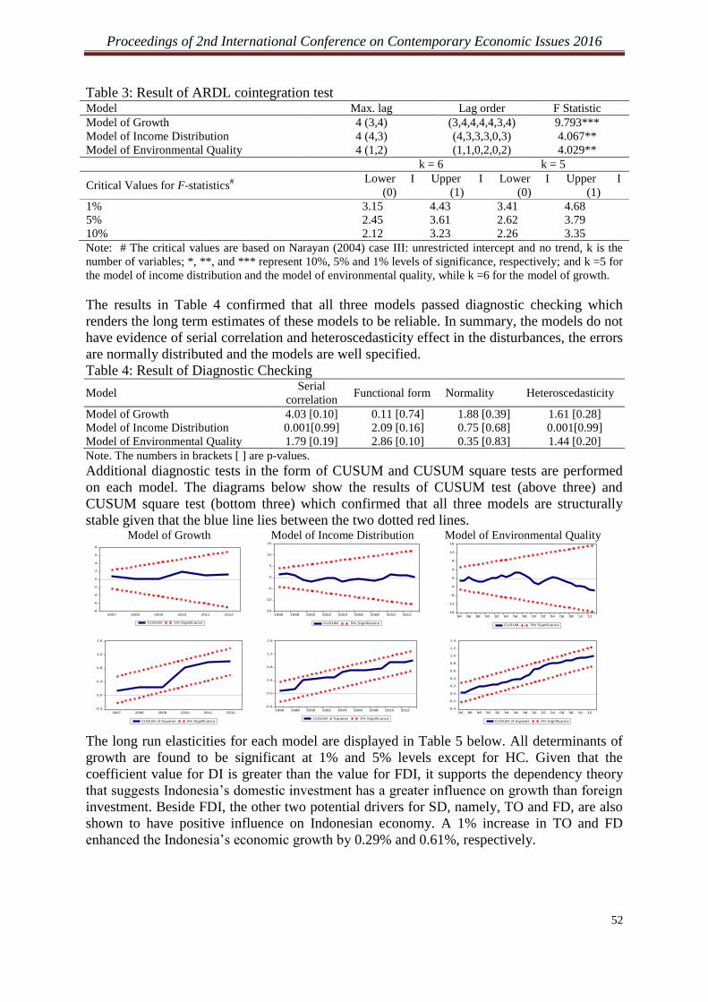
Proceedings of 2nd International Conference on Contemporary Economic Issues 2016
52
Table 3: Result of ARDL cointegration test Model Max. lag Lag order F Statistic
Model of Growth 4 (3,4) (3,4,4,4,4,3,4) 9.793***
Model of Income Distribution 4 (4,3) (4,3,3,3,0,3) 4.067**
Model of Environmental Quality 4 (1,2) (1,1,0,2,0,2) 4.029**
k = 6 k = 5
Critical Values for F-statistics#
Lower I
(0)
Upper I
(1)
Lower I
(0)
Upper I
(1)
1% 3.15 4.43 3.41 4.68
5% 2.45 3.61 2.62 3.79
10% 2.12 3.23 2.26 3.35
Note: # The critical values are based on Narayan (2004) case III: unrestricted intercept and no trend, k is the
number of variables; *, **, and *** represent 10%, 5% and 1% levels of significance, respectively; and k =5 for
the model of income distribution and the model of environmental quality, while k =6 for the model of growth.
The results in Table 4 confirmed that all three models passed diagnostic checking which
renders the long term estimates of these models to be reliable. In summary, the models do not
have evidence of serial correlation and heteroscedasticity effect in the disturbances, the errors
are normally distributed and the models are well specified.
Table 4: Result of Diagnostic Checking
Model Serial
correlation Functional form Normality Heteroscedasticity
Model of Growth 4.03 [0.10] 0.11 [0.74] 1.88 [0.39] 1.61 [0.28]
Model of Income Distribution 0.001[0.99] 2.09 [0.16] 0.75 [0.68] 0.001[0.99]
Model of Environmental Quality 1.79 [0.19] 2.86 [0.10] 0.35 [0.83] 1.44 [0.20]
Note. The numbers in brackets [ ] are p-values.
Additional diagnostic tests in the form of CUSUM and CUSUM square tests are performed
on each model. The diagrams below show the results of CUSUM test (above three) and
CUSUM square test (bottom three) which confirmed that all three models are structurally
stable given that the blue line lies between the two dotted red lines. Model of Growth Model of Income Distribution Model of Environmental Quality
-15
-10
-5
0
5
10
15
1996 1998 2000 2002 2004 2006 2008 2010 2012
CUSUM 5% Significance -16
-12
-8
-4
0
4
8
12
16
84 86 88 90 92 94 96 98 00 02 04 06 08 10 12
CUSUM 5% Significance
-0.4
0.0
0.4
0.8
1.2
1.6
2007 2008 2009 2010 2011 2012
CUSUM of Squares 5% Significance
-0.4
0.0
0.4
0.8
1.2
1.6
1996 1998 2000 2002 2004 2006 2008 2010 2012
CUSUM of Squares 5% Significance -0.4
-0.2
0.0
0.2
0.4
0.6
0.8
1.0
1.2
1.4
84 86 88 90 92 94 96 98 00 02 04 06 08 10 12
CUSUM of Squares 5% Significance
The long run elasticities for each model are displayed in Table 5 below. All determinants of
growth are found to be significant at 1% and 5% levels except for HC. Given that the
coefficient value for DI is greater than the value for FDI, it supports the dependency theory
that suggests Indonesia’s domestic investment has a greater influence on growth than foreign
investment. Beside FDI, the other two potential drivers for SD, namely, TO and FD, are also
shown to have positive influence on Indonesian economy. A 1% increase in TO and FD
enhanced the Indonesia’s economic growth by 0.29% and 0.61%, respectively.
-8
-6
-4
-2
0
2
4
6
8
2007 2008 2009 2010 2011 2012
CUSUM 5% Significance

Proceedings of 2nd International Conference on Contemporary Economic Issues 2016
53
Table 5: Estimation of Long-Run Elasticities Model of Growth Model of Income Distribution Model of Environmental Quality
Variables Coefficient Variables Coefficient Variables Coefficient
LNLAB 0.809*** LNGDP 1.129*** LNGDP 0.670*
LNDI 0.446*** LNDI -1.744** LNFDI -0.121**
LNFDI 0.077** LNFDI -0.155* LNFD 0.351***
LNHC 0.005 LNTO 0.432 LNEN 0.141
LNTO 0.610*** LNFD -0.415*** LNTO 0.444*
LNFD 0.293*** C -3.394*** C -9.285***
C -7.191***
Note: (*), (**), (***) indicate significant at 10%,5% and 1% significance level respectively.
According to Levine (1997), a more developed financial system in the country will give
fertile ground for better allocation of resources, better monitoring, more information
symmetry, and higher economic growth. Next, based on the model of income distribution, it
confirmed that DI, FDI, and FD could improve the income equality while higher GDP could
worsen the income equality in the country. TO, on the hand, failed to show any significant
impact on the model. Given that FDI has a negative and significant relationship with GINI, it
thus confirmed the validity of Mundell hypothesis which stated that increasing existing
amount of capital in the host country will lead to a rise in the marginal physical product of
labor and this in turn, will lead to a rise in wages. According to Arora (2012), the contribution
of FD can be the result of the financial sector’s ability to provide loans at a cheaper cost to
farmers to promote rural economy that lowers income inequality and hence reduce poverty.
Based on the model of environmental quality, it is shown that higher FDI inflows could
reduce the environmental degradation at 5% level of significance. FDI may have a negative
effect on CO2 emission when FDI facilitated the adoption of modern technologies during the
production process and ensure best environmental practices that lead towards higher energy
efficiency, better knowledge transfer, improved labor training, more skill acquisition and the
introduction of alternative management practices (Prakash and Potoski, 2007). FD and TO,
on the other hand, may worsen the environmental quality in Indonesia. TO may increase the
pollution levels because pollution is generated by the production of goods to fulfill the
consumption of another country through international trade. Surprisingly, there is no
relationship detected between EN and CO2 emission in this country.
Lastly, Table 6 reveals the outcome for short-run elasticities. Based on lag 0, for a model of
growth, FDI is found to positively influence the Indonesia’s economic growth. TO on the
other hand, has negatively influenced the growth. Based on the model of income distribution,
an increase in GDP, TO, and FD could worsen the income distribution in Indonesia, while DI
and FDI have managed to improve the country’s income distribution. Lastly, based on the
model of environmental quality, higher FDI inflow has successfully reduced the release of
CO2 emission. The long run relationship was supported by the negative and significant value
of error correction term (ECT) for each model. ECT reflects the speed of adjustment for each
model and the negative value means that the variables in each model will converge in the
long run. The highest speed of adjustment is detected for a model of growth (-0.90), followed
by a model of environmental quality (-0.51) and model of income distribution (-0.33).
Approximately, 90 percent, 51 percent and 33 percent disequilibria from the previous year’s
shock converge back to the long run equilibrium in the current year. Overall, the R-square
values for all three models suggest that almost 99 percent and 96 percent of the variables in
equations for Indonesia explains the dependent variables (GDP, GINI, and CO2).

Proceedings of 2nd International Conference on Contemporary Economic Issues 2016
54
Table 6: Estimation of Short Run Restricted Error Correction Model (ECM) Model of Growth Model of Income Distribution Model of Environmental Quality
Variables Coefficient Variables Coefficient Variables Coefficient
ΔLNGDPt-1 -0.021 Δ LNGINIt-1 0.513*** ΔLNGDPt 1.235***
ΔLNGDPt-2 -0.510** Δ LNGINI t-2 0.467** ΔLNFDIt -0.062**
ΔLNLABt -0.097 Δ LNGINIt-3 -0.381** ΔLNFDt 0.179
ΔLNLABt-1 0.160 Δ LNGDPt 0.760*** ΔLNFDt-1 -0.310**
ΔLNLABt-2 -0.685** Δ LNGDPt-1 -0.444 ΔLNENt 0.073
ΔLNLABt-3 -0.319 Δ LNGDPt-2 0.720*** ΔLNTOt 0.179
ΔLNDIt 0.131 Δ LNDIt -0.402*** ΔLNTOt-1 0.128
ΔLNDIt-1 -0.029 Δ LNDIt-1 -0.160 ECTt-1 -0.513***
ΔLNDIt-2 0.075 Δ LNDIt-2 0.343**
ΔLNDIt-3 -0.396* Δ LNFDIt -0.063**
ΔLNFDIt 0.112*** Δ LNFDIt-1 0.002
ΔLNFDIt-1 0.008 Δ LNFDIt-2 -0.033**
ΔLNFDIt-2 0.056** Δ LNTOt 0.146*
ΔLNFDIt-3 0.040** Δ LNFDt 0.377**
ΔLNHCt 0.020 Δ LNFDt-1 0.212
ΔLNHCt-1 -0.047 Δ LNFDt-2 0.205*
ΔLNHCt-2 0.078* ECTt-1 -0.339**
ΔLNHCt-3 -0.096**
ΔLNTOt -0.138**
ΔLNTOt-1 -0.171**
ΔLNTOt-2 -0.343***
ΔLNFDt -0.040
ΔLNFDt-1 -0.398**
ΔLNFDt-2 -0.069
ΔLNFDt-3 0.112
ECTt-1 -0.909***
R square 0.99 R square 0.96 R square 0.99
Ad.R square 0.99 Ad.R square 0.92 Ad.R square 0.99
Note: (*), (**), (***) indicate significance at 10%, 5% and 1% levels, respectively. Ad.R refers to adjusted R-
square.
5. Conclusion and Policy Recommendation
The impact of globalization on SD in Indonesia has been examined in this research. Among
the three characteristics of globalization, FDI inflows are seen as the most suitable candidate
to qualify as potential driver for SD in Indonesia as it has led to higher growth, reduced
income inequality and improved environmental quality based on the sample studied. FD, on
the other hand, only brings about positive impact on two out of the three pillars of SD,
namely, growth and income distribution. Meanwhile, TO is found to only bring positive
impact on growth, but has caused harm to the environmental quality, just like FD. As for
policy recommendation, considering “green economy” initiatives in trade liberalization
polices, it is perhaps most crucial for the government to pursue policies that work towards
reducing the country’s pollution. Towards that end, the government should give more
incentives in the form of tax exemptions for banks that provide loans to firms which get
involved in environmentally friendly investment projects in Indonesia.
Acknowledgement:
We wish to extend our gratitude to the School of Social Science, Universiti Sains Malaysia
for sponsoring the conference fees for this paper.
References
Arora, R.U., 2012. Finance and inequality: a study of Indian states. Applied Economics, 44,
pp.4527–4538.

Proceedings of 2nd International Conference on Contemporary Economic Issues 2016
55
Basu, P., and Guariglia, A., 2007. Foreign direct investment, inequality, and growth. Journal
of Macroeconomics, 29, pp.824–839.
Barro, R., and Lee, J.W., 2011. Educational attainment dataset. Available
at:<http://www.barrolee.com> Accessed 4 Jan 2016]
CO2 time series 1990-2014 per region/country dataset, 2015. Emissions Database for Global
Atmospheric Research [online] Available
at:<http://edgar.jrc.ec.europa.eu/overview.php?v=CO2ts1990-2014> [Accessed 2 Jan
2016].
Estimated Household Income Inequality dataset, 2008. University of Texas Income
Inequality Project [online]Available at:< http://utip.gov.utexas.edu/data.html> [Accessed
17 May 2015].
Income Inequality dataset, 2015. Global Consumption and Income Project [online] Available
at:< http://gcip.info/graphs/download> [Accessed 12 February 2016].
International Labor dataset, 2015. International Labor Organization. [online] Available at:<
http://www.ilo.org/global/statistics-and-databases/lang--en/index.htm>[Accessed 26
February 2016]
Klasra, M.A., 2011. Foreign direct investment, trade openness and economic growth in
Pakistan and Turkey: an investigation using bounds test. Quality and Quantity, 45,
pp.223–231.
Lee, J.E., 2006. Does globalization matter to income distribution in Asia? Applied
Economics Letter. 13, pp.851-855.
Lee, W.J., 2013. The contribution of foreign direct investment to clean energy use, carbon
emission and economic growth. Energy Policy. 55, pp.483-489.
Levine, R., 1997. Financial development and economic growth: views and agenda. Journal of
Economic Literature, 35, pp.688–726.
Mah, J.S., 2003. A note on globalization and income distribution - the case of Korea. Journal
of Asian Economics, 14(1), pp.161–168.
Mushtaq, M., Ahmad, K., Ahmed, S., and Nadeem, M., 2014. Impact of FDI on income
distribution in selected SAARC countries. Journal of Applied Environmental and
Biological Science, 4, pp.1–10.
Narayan, P.K., 2004. Reformulating critical values for the bound F- statistic: approach to
cointegration: an application to the tourism demand model for Fiji., Discussion Paper,
Monash University, Australia
Prakash, A., and Potoski, M., 2007. Investing up: FDI and the cross-country diffusion of ISO
14001management systems. International Studies Quarterly, 51(3), 723–744.
Shahbaz, M., Hye, Q.M.A., Tiwari, A. K., and Leitão, N.C., 2013. Economic growth, energy
consumption, financial development, international trade and CO2 emissions in Indonesia.
Renewable and Sustainable Energy Reviews, 25, pp.109–121.
Solarin, S.A., and Shahbaz, M., 2015. Natural gas consumption and economic growth: the
role of foreign direct investment, capital formation and trade openness in Malaysia.
Renewable Sustainable Energy Review, 42, pp.835–845.
World Bank. 2015. World Development Indicators. [online] Available at:
<http://databank.worldbank.org/data/download/archive/WDI_excel_2015_04.zip>
[Accessed 2 April 2015].
World Commission on Environment and Development. 1987. Our Common Future (The
Brundtland Report), Oxford University Press, Oxford.

Proceedings of 2nd International Conference on Contemporary Economic Issues 2016
56
A Seasonal Approach on Energy Consumption
Demand Analysis in Thailand
Sakkarin Nonthapot
Economics Program, Faculty of Integrated Social Sciences,
Khon Kaen University, Nong Khai Campus, Thailand
Email: [email protected]
Abstract
This study investigates the energy consumption demand in Thailand by using seasonal factors
in the analysis. The quarterly data from 2000-2014 which are analyzed by employing the
Seasonal Unit Root test, the Cointegration test and the Dynamic Ordinary Least Squares
(DOLS) procedures. The results show that all variables are stationary as in the same order
integration at I(1, 0, 0). The model is cointegrated. The income factor is positively related to
the energy consumption demand in Thailand in both the short run and the long run. Seasonal
factors affect the energy consumption demand in only the short run. Therefore, energy
consumption in Thailand depends on the income level. Energy policymakers should maintain
energy prices at a stable level, develop renewable energy and implement efficient green
energy for the upper middle income group to be an alternative energy policy in Thailand.
Keywords: Energy; energy consumption; seasonal unit root; demand of energy.
1. Introduction At present, billions of people depend on having access to reliable energy and water sources,
but due to rising energy costs and limited funds (World Energy Outlook. 2004), there are
many countries in the world that have difficulty meeting their energy needs without falling
into debt. Energy services are a basic human need and also contribute to economic
development in many sectors.
With rising costs of energy, many developing countries are also facing inefficiencies in the
energy management of the limited supply because energy management has limited experience
with energy conservation, and poor maintenance in energy provision. Hence, each developing
country needs to import raw energy and renewable energy. In particular, Thailand is a
developing country that needs to address these energy consumption issues. Because Thailand
has experienced a period of economic growth since the 1980’s, the country has become more
industrialized, and the demand for electricity and the consumption of energy have both risen.
Thailand is a small developing country located in Southeast Asia. Thailand has been
characterized by a high import/GDP ratio; accompanied by a weak productive sector and a
relatively stagnant export sector. In addition to this, during the last few years, the
development process in Thailand has been constrained by increased foreign debt servicing
and declining foreign exchange reserves because of the decline in the inflow of Southeast
Asia aid and worker remittances.
The energy consumption of Thailand is consumed by many sectors such as socio-economic
activities, households, industries and the improvement of infrastructure. Especially, electric
energy was a significance of economic driving in Thailand (Kandananond, 2011). These
continuously contribute to increase energy demand. It should be noted that energy imports
amounted to approximately 1,380.89 billion baht in 2013 while the total import value average

Proceedings of 2nd International Conference on Contemporary Economic Issues 2016
57
was 6,087.11 billion baht during 2006-2013 (see Table 1). Therefore, this sharp increase in
energy imports is linked to demand for energy consumption.
Table 1: Volume of Imports in Goods & Services and Energy Years Import Goods & Services Energy
2006 4,942.92 4,021.72 921.2
2007 4,870.19 3,988.17 882.01
2008 5,962.48 4,787.25 1,175.23
2009 4,601.98 3,825.08 776.91
2010 5,856.59 4,906.29 950.3
2011 6,982.72 5,761.38 1,221.34
2012 7,813.06 6,391.08 1,421.98
2013 7,666.93 6,286.04 1,380.89
Average 6,087.11 4,995.88 1,091.23
Note: Unit, billion baths
Source: Energy Policy and Planning Office (2014)
Generally, econometric models of energy demand are widely employed to provide income
and price elasticities because time series data are appropriate for such investigation as a result
of the nature of the samples from which the data is obtained. Pindyck (1980) and Bohi (1981)
previously studied the demand for energy in industrialized countries, whereas more recent
work has addressed the same problems by using primarily error correction methods. Few
studies have been directed towards investigating the demand for energy in developing
countries such as Dahl (1994), Balabanoff (1994) and Eltony and Al-Mutairi (1995). Previous
studies in energy consumption demand have not focused on seasonality especially in
Thailand. It is because Thailand is a developing country with a high level of energy
consumption (Pongthanaisawan, Sorapipatana, and Limmeechokchai, 2007) and the volume
of Thailand's using energy is gradually increasing (Ueasin, et al., 2015). In addition, Thailand
is located in a tropical zone so it may consume more energy in the summer than in other
seasons.
Hence, the purpose of this study is to investigate an advanced long run model or cointegrated
relationship by including seasonal factors in the demand for energy consumption in Thailand.
The findings of the research will present an alternative energy consumption demand model
and can be a planning guideline for policymakers. This study has been divided into four
sections. Section two contains the theoretical model and econometric methodologies. The
data and empirical results are discussed in Section three. Finally, this paper presents
conclusions and policy implications.
2. Data This study uses data that are related to the period 2000 to 2014 and were obtained from
various sources. Quarterly data on aggregate energy consumption (barrels), diesel and
liquefied petroleum gas (LPG) prices (billion baths) were collected from statistical reported
by the Energy Forecast and Information Technology Center of Thailand. Real Gross
Domestic product (Real GDP) (billion baths) data were collected from the Office of the
National Economic and Social Development Board of Thailand.
3. Methodology
3.1. Model A log linear specification is employed to represent the long-run demand for the energy
consumption model. Own price, income level and substitute price factors are included in the
Proceedings of 2nd International Conference on Contemporary Economic Issues 2016
58
independent variables, which follows demand theory. Generally, energy consumption demand
model is presented in a natural logarithm model as follows:
ttttt εPGlnβYlnβPDlnβαQln 321 (1)
where
tQ is aggregate energy consumption at time t
tPD is the real price of diesel per litter at time t
tY is real income (real Gross Domestic Products at the base year 2005) at time t
tPG is the real price of liquefied petroleum gas per kg. at time t α is a constant term
31 βtoβ are total energy demand elasticities.
tε is white noise term at time t
In equation (1), the parameter coefficients may be interpreted as elasticities which have to be
estimated with an estimating procedure under ideal conditions (i.e., tu is assumed to be an
identically and independently distributed (i.i.d.) white noise series. The expected signs of the
parameters are assumed to be 01 β , 2β and 03 β .
The sample period of the study corresponds to the quarterly data sets of the first quarter of
2000 to the fourth quarter of 2014, which adequately covers the turning point periods over 15
years (60 quarters). However, equation (1) lacks seasonal factors in the quarterly energy
consumption of each season. We assume a multiplicative seasonal form Eq. (1) which can
simply be transformed by being extended to capture the seasonal effects to come up with Eq.
(2).
tttttttt εDθDθDθPGlnβYlnβPDlnβαQln 332211321 (2)
For equation 2, the seasonal dummy variables 1ijD when the t period is the quarter ith
( 3,2,1i ) zero otherwise, and i represents the differential seasonal effect of the quarter
ith
relative to the fourth quarter, which in this model is the base quarter. Without this
extension, a certain form of omitted variable bias will occur if there truly is seasonality in the
quarterly energy consumption of Thailand, whereby estimates of the elasticity parameters will
be suspect.
3.2. Seasonal Unit Root Test The most important features in the time series data used in a research are the estimation and
inference procedures with a spurious regression problem. This problem is often found when
we use non-stationary data in the analysis. In this study, all of the variables used are known
(or at least suspected) to be non-stationary, particularly the dependent variable (energy
consumption) which is expected to exhibit significant seasonal tendencies.
The way to counter the spurious regression problem is the cointegration process.
Cointegration is the property of a group of time series data which are attached in one or more
long run equilibrium relationship. When the group of time series are cointegrated, although
the series is non-stationary, we can explain the series in both the short and long run together.
Normally, most series are said to be “integrated of order 1 or I(1) since a great majority of
available historical time series data have only one unit root, that are I(1). I(0) is the series that
is stationary. Hence, when the model has cointegration, it can be captured by undertaking an
error correction analysis which presents the speed adjustment of the estimated result from the
short run relationship to the long run relationship.

Proceedings of 2nd International Conference on Contemporary Economic Issues 2016
59
Seasonal variables should be considered as they are an integral part of the data. The usual
way for the cointegration procedure is to address the presence of seasonality in the data.
Hylleberg, Engle, and Granger (1990) developed an empirical procedure known as the HEGY
test. A seasonal time series has distinct peaks and troughs at seasonal frequencies. The type
of seasonal unit root implies that the seasonal pattern is changing and has to be captured for
the model to be reflective of the available information.
For a quarterly time series, say tx , a simple univariate model reflects its integration in all
seasonal and long run frequencies and is represented by the following equation: ttxL 41 (3)
where t is white noise for all t in the sample period. L is the lag operator. The series tx will
be integrated if seasonal unit roots are present in the transformed series suggested by equation
(3).The seasonal differencing operator 41 L can be factored mathematically as
4(1 ) (1 )(1 )(1 )(1 ) (1 ) ( )L L L iL iL L B (4)
The roots of the above equations can be ascertained at 1, -1 and a pair of complex roots
which correspond to a root at zero frequency, half- annual frequency and annual frequency,
respectively.
The term 1 L is used to isolate the unit roots at zero frequency and the lag polynomial
( )L is used to remove the seasonal unit roots. The HEGY test assumes that the series is
generated by a stochastic process 4( ) (1 )t t tL x L x (5)
From equation (5), for quarterly time series tx the HEGY auxiliary regression model to test
for the presence of seasonal unit roots is presented as:
*
4 1 1 1 2 2 1 3 3 2 4 3 1( ) t t t t t tL y y y y y (6)
where, 2 3
1 (1 )t ty L L L x , which maintains unit root at zero frequency and removes
seasonal roots; 2 3
2 (1 )t ty L L L x , which maintains bi-annual unit root and removes all other
roots; 2
3 (1 )t ty L x , which preserves the complex conjugates at annual
frequency; 4
4 (1 )t ty L x = 4t tx x , which is the quarterly different original series.
Empirical estimation of Equation (6) requires the augmentation of lagged 4ty to whiten the
stochastic error term t for the OLS procedure to be appropriate. If all 's are different
from zero, tx is stationary at all frequencies. The test for the presence of unit root at zero
frequency will be a t-test on the null of 1 0 . A t-test on the null 2 0 will determine the
presence of semi-annual unit root. A Wald type F-test on the joint hypothesis 3 4 0
will determine the annual cycle roots. If both of the last two tests are significant, seasonal unit
roots are not present. Hylleberg, Engle, and Granger (1990) developed the critical values for
the aforementioned tests whose sampling distributions differ from the usual t and F statistics.

Proceedings of 2nd International Conference on Contemporary Economic Issues 2016
60
Four different auxiliary forms of Equation (6) are to be established in the implementation of
the HEGY test – (1) with intercept (2) with intercept and trend (3) with intercept and seasonal
dummies, and (4) with intercept, seasonal trend and seasonal dummies. In addition, the
HEGY produces reliable results when the four forms of the auxiliary model are consistent in
their results.
3.3. Cointegration Test This study employs the cointegration test of Saikkonen and Lütkepohl (2000a; 2000b) or SL
test. Thus, Equations 2 are tested by employing a co-integration test which is based on the
general model. Saikkonen and Lütkepohl (2000a; 2000b) explained that SL test shows the
critical values remain valid of a shift dummy variable included in the model and it also
excludes the trend term from the model. This is because the SL procedure is adopted with any
number of (linearly independent) dummies in the model this method is suitable for seasonal
dummy variables model (Nonthapot and Ueasin, 2014).
3.4. The Stock Watson Dynamic OLS (DOLS) Approach An alternative approach, which has certain advantages over both the OLS and the maximum
likelihood procedures, is the Dynamic Ordinary Least Squares (DOLS) approach by Stock
and Watson (Stock and Watson, 1993). Their method improves on OLS by coping with small
samples and dynamic sources of bias. Moreover, the Johansen (1991) method is uncovered
with parameter estimates in a single equation that are affected by any misspecifications in
other equations. Hence the DOLS is more appropriate than the Johansen method when we
employ a single model.Furthermore, the DOLS estimated result has accuracy and robustness
with an endogeneity problem of regression by the inclusion of leads and lags of the first
differences of the regressors as well as serially correlated errors by a Generalized Least
Squares (GLS) procedure. In addition, it has the same asymptotic optimality properties as the
Johansen distribution. Therefore, this study appliesthe DOLS method for the estimation of
dynamic energy consumption demand model.
4. Results
4.1 Seasonal Unit Root Before the specified structural models can be implemented to undertake both long run and
short run analyses of energy consumption demand in Thailand, the statistical properties of the
different variables will have to be investigated. Instead of undertaking the usual unit root tests
on the variables of the study to ascertain departures from stationarity, a seasonal unit root test
via the HEGY framework is undertaken on both the dependent variable and the regressors.
This analysis is necessitated by the quarterly data.
Table 2 presents the results of the HEGY Seasonal Unit Root tests of the different variables.
It is seen in the table that the presence of unit root in the zero frequency, or in the level value
of the variables in logarithmic form is empirically validated by the tests. This result indicates
that all variables are non-stationary with a single unit root in the zero frequency for all
auxiliary regression scenarios which means there are non-seasonal unit roots in the series.
The second hypothesis is rejected which implies that all variables are stationary at the semi-
annual frequency. Finally, the third hypothesis is rejected as all variables are stationary at the
annual frequency. Therefore, the first null hypothesis is not rejected whereas the second and
third null hypotheses are rejected, which means a quarterly time series may have a non-
seasonal unit root but there are not semi-annual and annual unit roots. The order of
integration of all variables are shown in Table 3 and are in the same order as I(1, 0, 0).
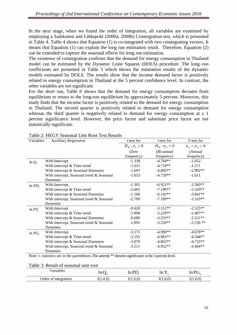
Proceedings of 2nd International Conference on Contemporary Economic Issues 2016
61
In the next stage, when we found the order of integration, all variables are examined by
employing a Saikkonen and Lütkepohl (2000a; 2000b) Cointegration test, which is presented
in Table 4. Table 4 shows that Equation (1) is co-integrated with two cointegrating vectors. It
means that Equation (1) can explain the long run estimation result. Therefore, Equation (2)
can be extended to capture the seasonal effects for long run estimation.
The existence of cointegration confirms that the demand for energy consumption in Thailand
model can be estimated by the Dynamic Least Squares (DOLS) procedure. The long–run
coefficients are presented in Table 5 which shows the estimation results of the dynamic
models estimated by DOLS. The results show that the income demand factor is positively
related to energy consumption in Thailand at the 5 percent confidence level. In contrast, the
other variables are not significant.
For the short run, Table 6 shows that the demand for energy consumption deviates from
equilibrium to return to the long-run equilibrium by approximately 5 percent. Moreover, this
study finds that the income factor is positively related to the demand for energy consumption
in Thailand. The second quarter is positively related to demand for energy consumption
whereas the third quarter is negatively related to demand for energy consumption at a 1
percent significance level. However, the price factor and substitute price factor are not
statistically significant.
Table 2: HEGY Seasonal Unit Root Test Results Variables Auxiliary Regression t-test for t-test for F-test for
0: 10 H
(Zero
frequency)
0: 20 H
(Bi-annual
frequency)
043
(Annual
frequency)
tQln With Intercept -1.338 -4.704** -1.652
With intercept & Time trend -1.651 -4.719** -1.571
With intercept & Seasonal Dummies -1.697 -4.885** -2.992**
With intercept, Seasonal trend & Seasonal
Dummies
-1.653 -4.729** -1.611
tPDln With Intercept -1.301 -6.921** -3.560**
With intercept & Time trend -2.601 -7.190** -3.320**
With intercept & Seasonal Dummies -1.160 -6.143** -3.841**
With intercept, Seasonal trend & Seasonal
Dummies
-2.709 -7.189** -3.319**
tPYln With Intercept -0.620 -3.151** -2.525**
With intercept & Time trend -1.890 -3.220** -2.487**
With intercept & Seasonal Dummies -0.680 -3.333** -2.521**
With intercept, Seasonal trend & Seasonal
Dummies
-1.891 -3.220** -2.536 **
tPGln With Intercept -3.171 -4.990** -4.678**
With intercept & Time trend -3.191 -4.981** -4.544**
With intercept & Seasonal Dummies -3.070 -4.862** -4.725**
With intercept, Seasonal trend & Seasonal
Dummies
-3.211 -4.952** -4.464**
Note: t- statistics are in the parentheses.The asterisk ** denotes significance at the 5 percent level.
Table 3: Result of seasonal unit root Variables
tQln tPDln tYln tPGln
Order of integration I(1,0,0) I(1,0,0) I(1,0,0) I(1,0,0)
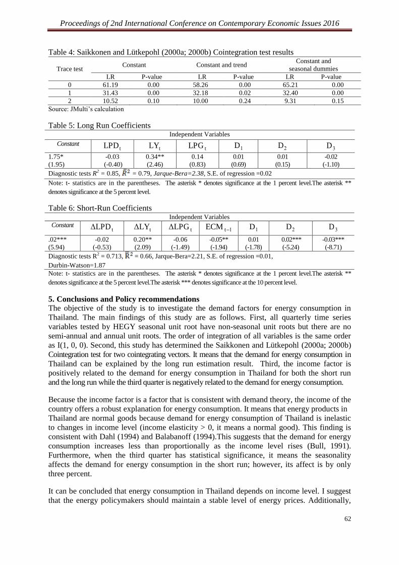
Proceedings of 2nd International Conference on Contemporary Economic Issues 2016
62
Table 4: Saikkonen and Lütkepohl (2000a; 2000b) Cointegration test results
Trace test Constant Constant and trend
Constant and
seasonal dummies
LR P-value LR P-value LR P-value
0 61.19 0.00 58.26 0.00 65.21 0.00
1 31.43 0.00 32.18 0.02 32.40 0.00
2 10.52 0.10 10.00 0.24 9.31 0.15
Source: JMulti’s calculation
Table 5: Long Run Coefficients Independent Variables
Constant tLPD tLY tLPG 1D 2D 3D
1.75*
(1.95)
-0.03
(-0.40)
0.34**
(2.46)
0.14
(0.83)
0.01
(0.69)
0.01
(0.15)
-0.02
(-1.10)
Diagnostic tests R2 = 0.85, = 0.79, Jarque-Bera=2.38, S.E. of regression =0.02
Note: t- statistics are in the parentheses. The asterisk * denotes significance at the 1 percent level.The asterisk **
denotes significance at the 5 percent level.
Table 6: Short-Run Coefficients Independent Variables
Constant tLPDΔ tLYΔ tLPGΔ 1tECM 1D 2D 3D
.02***
(5.94)
-0.02
(-0.53)
0.20**
(2.09)
-0.06
(-1.49)
-0.05**
(-1.94)
0.01
(-1.78)
0.02***
(-5.24)
-0.03***
(-8.71)
Diagnostic tests R2 = 0.713, = 0.66, Jarque-Bera=2.21, S.E. of regression =0.01,
Durbin-Watson=1.87
Note: t- statistics are in the parentheses. The asterisk * denotes significance at the 1 percent level.The asterisk **
denotes significance at the 5 percent level.The asterisk *** denotes significance at the 10 percent level.
5. Conclusions and Policy recommendations The objective of the study is to investigate the demand factors for energy consumption in
Thailand. The main findings of this study are as follows. First, all quarterly time series
variables tested by HEGY seasonal unit root have non-seasonal unit roots but there are no
semi-annual and annual unit roots. The order of integration of all variables is the same order
as I(1, 0, 0). Second, this study has determined the Saikkonen and Lütkepohl (2000a; 2000b)
Cointegration test for two cointegrating vectors. It means that the demand for energy consumption in
Thailand can be explained by the long run estimation result. Third, the income factor is
positively related to the demand for energy consumption in Thailand for both the short run
and the long run while the third quarter is negatively related to the demand for energy consumption.
Because the income factor is a factor that is consistent with demand theory, the income of the
country offers a robust explanation for energy consumption. It means that energy products in
Thailand are normal goods because demand for energy consumption of Thailand is inelastic
to changes in income level (income elasticity > 0, it means a normal good). This finding is
consistent with Dahl (1994) and Balabanoff (1994).This suggests that the demand for energy
consumption increases less than proportionally as the income level rises (Bull, 1991).
Furthermore, when the third quarter has statistical significance, it means the seasonality
affects the demand for energy consumption in the short run; however, its affect is by only
three percent.
It can be concluded that energy consumption in Thailand depends on income level. I suggest
that the energy policymakers should maintain a stable level of energy prices. Additionally,

Proceedings of 2nd International Conference on Contemporary Economic Issues 2016
63
they should develop renewable energy and offer green energy for the upper middle-income
group as alternative energy policy in Thailand.
References Balabanoff, S., 1994. The dynamics of energy demand in Latin America, OPEC Review, 18,
476-488.
Bohi, R. D., 1981. Analysing demand behaviour, a study of energy elasticity, resources for
the future, Baltimore: John Hopkin University Press.
Bull, A., 1991. The economics of Travel and Tourism. (2nd ed). Melbourne: Addison
Wesley Longman.
Dahl, C, 1994. A survey of Energy Demand Elasticities for the Developing World, The
Journal of Energy and Development, 18, 1-47.
Eltony, M and Al-Mutairi, N., 1995. Demand for gasoline in Kuwait an empirical analysis
using Cointegration techniques, Energy economics. 7(3), 249-253.
Energy Policy and Planning Office. 2014. Energy statistics. [online]. Available at:
<http://www.eppo.go.th/info/index-statistics.html> [Accessed on 20 May 2015]
Hylleberg, S., Engle, R. and Granger, C.W., 1990. Seasonal Integration and Cointegration.
Journal of Econometrics, 44, 215-238.
Johansen, S., 1991. Estimating and hypothesis testing of cointegrating vectors autoregressive
models. Econometrica, 59. 1551-1589.
Kandananond, K., 2011. Forecasting electricity demand in Thailand with an artificial neutral
network approach. Energies. 4, 1246-1257.
Nonthapot, S. and Ueasin, N., 2014.The impact of Thai tourism on the economic growth of
tourism in Lao PDR: A hierarchical approach. TOURISMOS: An International
Multidisciplinary Journal of Tourism, 9(2), 67-82.
Pindyck, R.S., 1980.The structure of world energy demand. Cambridge: MIT press.
Pongthanaisawan, J., Sorapipatana, C. and Limmeechokchai, B. 2007. Road transport energy
demand analysis and energy saving potentials in Thailand, Asian Journal on Energy and
Environment, 8 (1-2), 49-72.
Saikkonen, P. and Lütkepohl, H., 2000a. Testing for the cointegrating rank of a VAR
process with an intercept. Econometric Theory, 16, 373-406.
Saikkonen, P. and Lütkepohl, H., 2000b. Testing for the cointegrating rank of a VAR process
with structural shifts. Journal of Business & Economic Statistics, 18, 451-464.
Stock, J. and Watson, M. W., 1993. A simple estimator of cointegrating vectors in higher
order integrated systems. Econometrica, 61(4), 783-820.
Ueasin, N., Wongchai, A. and Nonthapot, S., 2015. Performance Assessment and
optimization of Biomass Steam Turbine Power Plants by Data Envelopment Analysis.
International Journal of Energy Economics and Policy, 5(3), 668-672.
World Energy Outlook, 2004. Energy and Development. International Energy Agency,
[online] February Available at: http://www.worldenergyoutlook.org/database
electricity/WEO2004-haper%2010.pdf> [Accessed on 6 Oct 2015].
Proceedings of 2nd International Conference on Contemporary Economic Issues 2016
64
Motives for Demand for Religion: A Confirmatory Factor Analysis
Sotheeswari Somasundrama,
*, Muzafar Shah Habibullahb
aTaylor’s University, Malaysia
Email: [email protected]
bUniversiti Putra Malaysia, Malaysia
Abstract
This study investigates the motivation for religious demand among Christians using the
International Social Survey Program (ISSP) data on Religion for 2008. This study using both
exploratory and confirmatory factor analysis identified two motives, afterlife motive and the
current life motive that influences demand for religion. The afterlife motive, aligned to the
Christian doctrine of belief in afterlife, heaven and hell, was one of the dimensions of
motives for religious demand. For gains in the current life, although the various studies
highlight two construct of personal gains and social gains, however, for this study, all items
loaded onto only one construct, which is broadly termed as current life motives where
religion is said to provide solace, inner peace; as well as social support and networking
opportunities.
Keywords: Religion; economics; demand; afterlife; current life.
1. Introduction
The interdisciplinary studies of economics and religion was initially explored by Adam Smith
in the Wealth of Nations (Smith 1976), where economic principles such as demand and
supply theories5 were applied to explain the participation of rational individuals in the
religious market. Following the work of Adam Smith, the subsequent publication was the
study of allocation of time between consumption products and afterlife products using the
household production model by Azzi & Ehrenberg (1975). The first and second publication
had a gap of almost two centuries (Iannaccone 1998). The paper by Azzi & Ehrenberg (1975)
is considered as the seminal paper which was instrumental in creating a renewed interest in
this subfield of economics.
Smith (1976) in the Wealth of Nations deliberated on the economic incentives accruing to
religious practitioners adhering to the moral code of conduct propagated by religious
doctrines. Religious belief is seen as an “internal moral enforcement mechanism”(Anderson
1988, p.1069) which reinforces the need to abide by moral strictures and practice self-
restraint. According to Smith (1976) it is important to adhere to strict moral obligations if an
individual wants to gain the respect of society. The question is how does the reinforcement of
self-restraint arising from religious belief provides economic incentives to religious
practitioners. Anderson (1988) in expounding Adam Smith’s proposition highlights that
moral reputation is an indication of the human capital worth of an individual. Someone
5 In the Wealth of nation, Adam Smith explored both demand and supply side of religion, where for demand
side the participation in religion was seen as contributing to human capital (Anderson 1988). Iannaccone (1990)
adopted this concept and incorporated the human capital analysis in the demand model. For the supply side
analysis, Adam Smith described the behavior of suppliers of religious services such as churches from an
economic perspective, where the churches were seen as monopolies with rent seeking activities by clergies
(Anderson 1988).
Proceedings of 2nd International Conference on Contemporary Economic Issues 2016
65
abiding to moral strictures as ordained by religious doctrines would be perceived as a highly
moral person which enhances his/her human capital worth. Thus, the economic incentive for
demand for religion is a higher capital value of an individual resulting from high moral
reputation. The aim of this study is to examine the motives for demand for religion in relation
to economic incentives. Given that economic incentives are key drivers of religious demand,
the proposition of this study is that a better understanding of motives for demand will not
only complement existing literatures but also provide an opportunity to identify other
possible economic incentives.
2. Literature Review
Both demand for religion and demand for secular products share many similarities. In the
case of secular products quantity demanded of a product is identified as a measure, while
demand for religion is expressed as the level of religious participation (Iannaccone et. al,
1997). One of the key motives for demand for religion is afterlife rewards. Azzi & Ehrenberg
(1975) used church attendance to represent demand for religion and concluded that afterlife
rewards influences the allocation of time between afterlife consumption and secular
consumption. Hrung (2004) replaced Azzi & Ehrenberg’s dependent variable of church
attendance with monetary contribution and concurred with Azzi & Ehrenberg that afterlife
rewards influence demand for religion. The motives for demand for religion are not
exclusively focused in the afterlife gains, as studies have highlighted that individuals seek
benefits in the current life as well. For current life gains, studies have focused on two aspects,
one is personal and the other social. For personal motives, studies have identified factors such
as extrinsic motivations such as providing “security and solace, sociability and distraction,
status and self-justification” (Allport & Ross 1967, p.434). Religion is seen among others as a
coping mechanism where it provides solace during times of sorrow (Harris et al., 2010;
Pargament, 2002) and providing assurance of better health, better financial position, or
generally to attain a better quality of life (Baker, 2008; Maltby, Lewis, & Day, 1999). For the
motive of social gains, religious participation is seen as creating a sense of belonging as well
as allowing individuals to establish a strong social network which provides both formal and
informal support (Ellison & George, 1994; Scheitle & Adamczyk, 2009) and allowing better
integration among the communities (Hurh & Kim 1990; Peifer 2010). In summary, the
existing studies highlight a number of afterlife and current life gains that motivates demand
for religion. Motives for afterlife demand are the perceived benefits that an individual expects
to gain in their afterlife. Demand for religion in the current life is motivated by personal gains
as well as social gains. Personal gains include among others the sense of security that
religion provides an individual during times of tribulation; or the reassurance of a better
quality of life in terms of better health or even a superior financial position. For social gains,
studies have highlighted community bonding, maintaining a social network, social integration
as a motivating factor for demand for religion.
3. Method
The data used in this study is from the International Social Survey Program (ISSP) 2008, an
international collaborative survey on religion (ISSP Research Group 2012). The survey
questioned respondents on their attitude towards religious practices. One of the challenges in
using the ISSP dataset is fitting the survey questions to the framework of the present study. In
order to align the survey questions to the concepts highlighted in the literature, the present
study will focus on operationalizing the motives by identifying items applied in existing
literatures which are similar to the questions covered in ISSP survey. For afterlife motive,
reference is made to the study by McCleary & Barro (2006) on salvific merits “which
connects the perceived probability of salvation to a person’s lifetime activities” (p.51).
Proceedings of 2nd International Conference on Contemporary Economic Issues 2016
66
Salvific merits which is the concept of afterlife rewards or punishments in accordance to an
individual’s behaviour in his/her lifetime is aligned to afterlife motive of the present study.
McCleary & Barro (2006) and Mccleary (2007) in exploring the salvific merits of Christians
included measures such as belief in heaven, belief in hell and belief in afterlife in their study.
These questions were included in the ISSP survey.
As shown in Table 1, the sequence of questions is as follows: Do you believe in… (a) Life
after death, (b) Heaven, and (c) Hell. The questions are Likert-scale items coded 1-5 with the
value of 1 representing a strong agreement of ‘yes definitely’. For the current life gains, the
present study refers to the Religious Orientation Scale (ROS) developed by Allport & Ross
(1967) and modified by Darvyri et al. (2014). The ROS focuses on intrinsic and extrinsic
orientations. For intrinsic orientation the practitioner internalize the teaching in an attempt to
live his/her life as what the religion preaches (Allport & Ross 1967). Extrinsic orientation is
focused towards non-religious outcomes where those with a high degree of extrinsic
orientation use religion as a means “to provide security and solace, sociability and distraction,
status and self-justification” (Allport & Ross 1967, p.434). The extrinsic orientation is
aligned to the current life motive proposed by the present study. In order to capture the
extrinsic motives, Darvyri et al. (2014) applied a revised ROS which included questions such
as “I go to church because it helps me to make friends”; “I go to church mostly to spend time
with my friends”, “I go to church mainly because I enjoy seeing people I know there” and
“What religion offers me most is comfort in times of trouble and sorrow”. In order to identify
questions which were aligned to the extrinsic orientation, the present study refers to questions
categorized as the “attitudes towards the profits of practicing a religion” (GESIS n.d.) in the
ISSP questionnaire. There were four questions in the ISSP questionnaire which were aligned
to the extrinsic orientation. As shown in Table 1, the sequence of questions were as follows:
Do you agree or disagree that practicing a religion helps people to… (a) find inner peace and
happiness, (b) make friends, (c) gain comfort in times of trouble or sorrow, and (d) meet the
right kind of people. The questions are Likert-scale items and are coded 1 -5 with the value of
1 representing a strong agreement of ‘strongly agree’.
According to ISSP Research Group (2012) the dataset captures the religious beliefs and
practices of Muslims, Christians, Buddhists, Jews, Hindus, eastern religions, Asian religions
and other religions. The present study is only focusing on the motives for demand for religion
among Christian, as such only relevant data will be extracted from the dataset. The data will
be divided into two groups. The responses of 1252 Christian respondents were extracted from
ISSP 2008 dataset which was divided into two groups, the first group is for exploratory factor
analysis and the second group is for confirmatory factor analysis. The respondents are from
Australia, Austria, Belgium, Chile, Croatia, Denmark, Finland, France, Ireland, Philippines,
United Kingdom and United States. The first group has 618 respondents (age range = 15 to
92, M = 49.76, SD = 17.03), 251 males and 367 females. Married respondents are 52%, 28%
are single and the remaining 20% are either divorced, widowed or separated. To gauge the
demand for religion, the question on frequency of prayer indicates that 30.2% prayed on a
daily basis, 23.8% prayed on a weekly basis, 9.9% prayed on a monthly basis, 21.5% prayed
once or twice in a year and 14.3% never pray. The second group has 634 respondents (age
range = 15 to 88, M = 48.43, SD = 17.5), 269 males and 365 females. Married respondents
are 53.1%, 29.7% are single and the remaining are either divorced, widowed or separated.
For the second group, 31.7% prayed on a daily basis, 23.7% prayed on a weekly basis, 8%
prayed on a monthly basis, 20.5% prayed once or twice in a year and 16.1% never pray.
Proceedings of 2nd International Conference on Contemporary Economic Issues 2016
67
4. Results
The study carried out both exploratory and confirmatory factor analysis. The seven items
were factored using principal component factor analysis with varimax rotation. Two criteria
were used to identify the number of factors and factor loadings for each item: an eigenvalue
greater than 1.0 and a factor loading greater than 0.5 (Chen & Tsai 2007; Schommer 1990) on
any one factor. Two constructs were identified: one is the afterlife motive and the other
current life motives. Table 2 on factor loadings indicates that all the items had factor loadings
greater than 0.7. The first factor explained 51.9% of the variance in the items (eigenvalue =
3.634). Items loading on the first factor are whether religion helps people find inner peace,
make friends, provide comfort and meet right kind of people. Although both Confirmatory
Factor Analysis (CFA) and EFA apply factor loadings as an analytical tool but conceptually
there are significant difference between the two approaches. For CFA, the number of
constructs and the items that are likely to load onto the construct need to be theoretically
supported. The present study, looked at existing literatures in proposing the hypothesis, and
then carried out an EFA to identify the constructs. The factor loading using CFA produced
similar results as EFA analysis where, the items loaded onto two constructs, current life
motives and afterlife motives. The factor loading is taken as one of the measures of reliability.
The criteria for acceptance is for four or more loadings of at least 0.6 regardless of sample
size. (Guadagnoli & Velicer 1988), but studies have applied factor loadings of above 0.5
(Chen & Tsai 2007; Schommer 1990). Table 3 shows the factor loadings are above 0.6 which
indicates that all seven items are adequate in their reliability individually.
In carrying out confirmatory factor analysis, it is important to determine if the factors exhibit
convergent and discriminant validity as well as reliability. If there are convergent validity
problem, this indicates that the items are unable to explain the latent variable, while for
discriminant validity it indicates that there are high correlation between items in of one
construct with another construct rather than within the same construct (Hair et al., 2010). The
threshold measures for validity and reliability as highlighted by Hair et al., (2010) are that the
composite reliability value (CR) must be greater than 0.7; to ensure convergent validity, the
average variance extracted (AVE) must be above 0.5; and for discriminant validity both
maximum shared variance (MSV), and average shared variance (ASV) must be less than
AVE. In addition, the square root of AVE must be greater than inter-construct correlations,
where constructs meeting these criteria are said to exhibit both validity and reliability. For
this study the CR, AVE, MSV and ASV values shows that both factors demonstrate
reliability as the CR value is greater than 0.7 for both constructs. The factors also exhibit
convergent validity where the AVE for both constructs are more than 0.5. In the case of
discriminant validity, the MSV and ASV values for both constructs are less than the AVE
value. The third measure for discriminant validity, which is square root of AVE must be
greater than correlation value, where the threshold is met for afterlife motive as AVE value is
above the correlation value. The construct for current life motive indicates that the AVE
value is equals to the squared root of correlation value. In this case, as three out of four
threshold values have been met and the AVE value is equals to squared root correlation value,
it is taken that the current life motive construct demonstrates discriminant validity.
5. Discussion
The proposition of this study is that there are two key motives for demand for religion. The
afterlife motive is where religious consumers seek a desired outcome exclusive to what is
prescribed by individual religions. This outcome is closely linked to the concept of a
salvation motive proposed by Azzi & Ehrenberg (1975) and the compensator idea proposed

Proceedings of 2nd International Conference on Contemporary Economic Issues 2016
68
by Bainbridge & Stark (1979). Individuals acknowledging that they believe in an after-life,
heaven or hell, outcomes are deemed to be expressing a desire to achieve the after-life
rewards promised by the Christian doctrines. The empirical findings of the present study is in
line with earlier studies that one of the motives for demand for religion is the perceived gains
in afterlife. For current life, religious consumers are motivated by benefits such as getting
solace or inner peace or materialistic gains such as better social status or better networking
opportunities. The case where individuals practice religion with the hope of receiving solace
or comfort in times of trouble or sorrow to “help cope with fear and to pass through crisis
situations”(Hubert 2015, p.39) is when individuals are seeking favourable outcome in
personal, family or work life. Individuals turn to religion to seek peace and happiness or to
obtain solace during times of sorrow, seeking strength and reassurance during period of
illness; they seek the reassurance of faith as a promise of better times during hardship and so
on. The empirical findings support the proposition of this study that one of the motives for
demand for religion is for peace and solace. The other items that loaded into the current life
motives are religion helps people make friends and religion helps people meet the right kind
of people which is linked to social support and networking opportunities. These items are
aligned to Azzi & Ehrenberg’s (1975) social pressure motives and Allport & Ross’s (1967)
extrinsic motivation. Religious consumers are subscribing and adhering to religious
requirements with the intention of gaining a favourable position with their congregation.
6. Conclusion
The focus of this study was to investigate the motives of demand for religion in relations to
the proposition of economic incentives proposed by Adam Smith in the Wealth of Nations
(Smith 1976). The findings of the present study are aligned to Adam Smith’s human capital
model. Adam Smith’s proposition is that individuals would adhere to strict moral strictures to
enhance their human capital worth which is supported by the current life motive proposition
of the present study. An individual deemed to be adhering and practicing in accordance to
religious doctrines would experience a better social standing within his/her religious circle.
The capital value of an individual is enhanced through his/her prominent presence in society.
This enhancement in capital worth would provide returns in the form of better engagements
and networking opportunities leading to material and professional gains. In addition to the
current life motive, this study has identified afterlife gains as a motive for demanding religion.
However, it is not within the scope of the present study to explore the economic incentives of
afterlife motives. Nevertheless, there is an opportunity for future research to study the
relationship between afterlife motives and economic incentives.
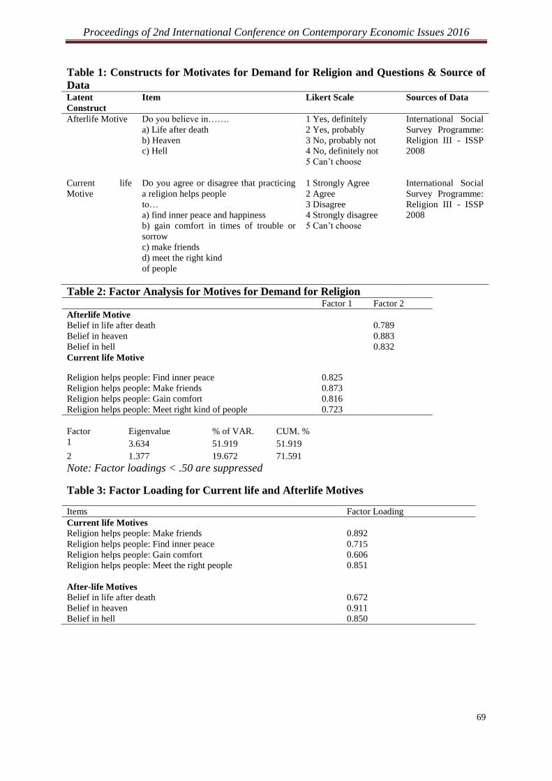
Proceedings of 2nd International Conference on Contemporary Economic Issues 2016
69
Table 1: Constructs for Motivates for Demand for Religion and Questions & Source of
Data Latent
Construct
Item Likert Scale Sources of Data
Afterlife Motive Do you believe in…….
a) Life after death
b) Heaven
c) Hell
1 Yes, definitely
2 Yes, probably
3 No, probably not
4 No, definitely not
5 Can’t choose
International Social
Survey Programme:
Religion III - ISSP
2008
Current life
Motive
Do you agree or disagree that practicing
a religion helps people
to…
a) find inner peace and happiness
b) gain comfort in times of trouble or
sorrow
c) make friends
d) meet the right kind
of people
1 Strongly Agree
2 Agree
3 Disagree
4 Strongly disagree
5 Can’t choose
International Social
Survey Programme:
Religion III - ISSP
2008
Table 2: Factor Analysis for Motives for Demand for Religion Factor 1 Factor 2
Afterlife Motive
Belief in life after death 0.789
Belief in heaven 0.883
Belief in hell 0.832
Current life Motive
Religion helps people: Find inner peace 0.825
Religion helps people: Make friends 0.873
Religion helps people: Gain comfort 0.816
Religion helps people: Meet right kind of people 0.723
Factor
Eigenvalue
% of VAR.
CUM. %
1 3.634 51.919 51.919
2 1.377 19.672 71.591
Note: Factor loadings < .50 are suppressed
Table 3: Factor Loading for Current life and Afterlife Motives
Items Factor Loading
Current life Motives
Religion helps people: Make friends 0.892
Religion helps people: Find inner peace 0.715
Religion helps people: Gain comfort 0.606
Religion helps people: Meet the right people 0.851
After-life Motives
Belief in life after death 0.672
Belief in heaven 0.911
Belief in hell 0.850
Proceedings of 2nd International Conference on Contemporary Economic Issues 2016
70
References
Allport, G.W. and Ross, J.M., 1967. Personal religious orientation and prejudice. Journal of
personality and social psychology, 5(4), pp.432–443. Available at:
http://doi.apa.org/getdoi.cfm?doi=10.1037/h0021212 [Accessed April 11, 2016].
Anderson, G.M., 1988. Mr. Smith and the Preachers: The Economics of Religion in the
Wealth of Nations. Journal of Political Economy, 96(5), pp.1066–1088. Available at:
http://www.jstor.org/stable/1837247 [Accessed April 11, 2016].
Azzi, C. and Ehrenberg, R., 1975. Household Allocation of Time and Church Attendance.
Journal of Political Economy, 83(1), pp.27–56. Available at:
http://www.jstor.org/stable/1833272 [Accessed April 11, 2016].
Bainbridge, W. and Stark, R., 1979. Cult formation: Three compatible models. Sociology of
Religion, 40(4), pp.285–295. Available at:
http://socrel.oxfordjournals.org/content/40/4/283.short [Accessed April 10, 2016].
Baker, J.O., 2008. An Investigation of the Sociological Patterns of Prayer Frequency and
Content. Sociology of Religion, 69(2), pp.169–185. Available at:
http://www.jstor.org/stable/20453213 [Accessed April 24, 2016].
Chen, C.-F. and Tsai, D., 2007. How destination image and evaluative factors affect
behavioral intentions? Tourism Management, 28(4), pp.1115–1122. Available at:
http://linkinghub.elsevier.com/retrieve/pii/S0261517706001397 [Accessed June 19, 2016].
Darvyri, P. et al., 2014. The Revised Intrinsic/Extrinsic Religious Orientation Scale in a
Sample of Attica’s Inhabitants. Psychology, 5(13), pp.1557–1567. Available at:
http://www.scirp.org/journal/psych [Accessed August 10, 2016].
Ellison, C.G. and George, L.K., 1994. Religious Involvement, Social Ties, and Social
Support in a Southeastern Community. Journal for the Scientific Study of Religion, 33(1),
pp.46–61. Available at: http://www.jstor.org/stable/1386636 [Accessed April 27, 2016].
GESIS, ZA4950: International Social Survey Programme 2008: Religion III (ISSP 2008).
Leibniz Institute for the Social Sciences. Available at:
http://zacat.gesis.org/webview/index.jsp?object=http://zacat.gesis.org/obj/fStudy/ZA4950
[Accessed December 24, 2016].
Guadagnoli, E. and Velicer, W.F., 1988. Relation to sample size to the stability of component
patterns. Psychological Bulletin, 103(2), pp.265–275. Available at:
http://doi.apa.org/getdoi.cfm?doi=10.1037/0033-2909.103.2.265.
Hair, J. et al., 2010. Multivariate Data Analysis 7th ed., Upper Saddle River, NJ, USA.:
Prentice-Hall, Inc.
Harris, J.I. et al., 2010. Coping Functions of Prayer and Posttraumatic Growth. International
Journal for the Psychology of Religion, 20(1), pp.26–38. Available at:
http://www.tandfonline.com/doi/abs/10.1080/10508610903418103 [Accessed April 27,
2016].
Hrung, W.B., 2004. After-Life Consumption and Charitable Giving. The American Journal of
Economics and Sociology, 63(3). Available at: http://www.jstor.org/stable/3488151
[Accessed April 24, 2016].
Hubert, S., 2015. Religion and Religiosity. In The Impact of Religiosity on Fertility.
Wiesbaden: Springer Fachmedien Wiesbaden, pp. 37–68. Available at:
http://link.springer.com/10.1007/978-3-658-07008-3_3 [Accessed April 21, 2016].
Hurh, W.M. and Kim, K.C., 1990. Religious Participation of Korean Immigrants in the
United States. Journal for the Scientific Study of Religion, 29(1), pp.19–34. Available at:
http://www.jstor.org/stable/1387028?origin=crossref [Accessed April 27, 2016].
Iannaccone, L., 1998. Introduction to the Economics of Religion. Journal of Economic
Literature, XXXVI, pp.1465–1496.
Proceedings of 2nd International Conference on Contemporary Economic Issues 2016
71
Iannaccone, L., 1990. Religious Practice: A Human Capital Approach. Journal of the
Scientific Study of Religion, 29(3), pp.297–314.
Iannaccone, L., Finke, R. and Stark, R., 1997. Deregulating Religion: The Economics of
Church and State. Economic Inquiry, 35(2), pp.350–364. Available at:
http://doi.wiley.com/10.1111/j.1465-7295.1997.tb01915.x.
ISSP Research Group, 2012. International Social Survey Programme: Religion III - ISSP
2008.
Maltby, J., Lewis, C.A. and Day, L., 1999. Religious orientation and psychological well-
being: The role of the frequency of personal prayer. British Journal of Health Psychology,
4(4), pp.363–378. Available at: http://doi.wiley.com/10.1348/135910799168704
[Accessed April 11, 2016].
Mccleary, R.M., 2007. Salvation, Damnation, and Economic Incentives. Journal of
Contemporary Religion, 22(1), pp.49–74. Available at:
http://www.tandfonline.com/doi/abs/10.1080/13537900601114503.
McCleary, R.M. and Barro, R.J., 2006. Religion and Economy. Journal of Economic
Perspectives, 20(2), pp.49–72. Available at:
http://pubs.aeaweb.org/doi/abs/10.1257/jep.20.2.49.
McIntosh, W.A. and Alston, J.P., 1982. Lenski Revisited: The Linkage Role of Religion in
Primary and Secondary Groups. American Journal of Sociology, 87(4), pp.852–882.
Available at: http://www.jstor.org/stable/2778781 [Accessed April 27, 2016].
Pargament, K.I., 2002. Is Religion Nothing But ...? Explaining Religion Versus Explaining
Religion Away. Psychological Inquiry Copyright ?), 13(3), pp.239–244.
Pargament, K.I. et al., 1988. Religion and the Problem-Solving Process: Three Styles of
Coping. Source Journal for the Scientific Study of Religion, 27(1), pp.90–104. Available
at: http://www.jstor.org/stable/1387404 [Accessed April 21, 2016].
Peifer, J.L., 2010. The Economics and Sociology of Religious Giving: Instrumental
Rationality or Communal Bonding? Social Forces, 88(4), pp.1569–1594. Available at:
http://www.jstor.org/stable/40645950 [Accessed April 24, 2016].
Poloma, M.M. and Pendleton, B.F., 1989. Exploring Types of Prayer and Quality of Life: A
Research Note. Review of Religious Research, 31(1), pp.46–53.
Scheitle, C.P. and Adamczyk, A., 2009. It Takes Two: The Interplay of Individual and Group
Theology on Social Embeddedness. Journal for the Scientific Study of Religion, 48(1),
pp.16–29. Available at: http://www.jstor.org/stable/20486978 [Accessed April 27, 2016].
Schommer, M., 1990. Effects of beliefs about the nature of knowledge on comprehension.
Journal of Educational Psychology, 82(3), pp.498–504. Available at:
http://doi.apa.org/getdoi.cfm?doi=10.1037/0022-0663.82.3.498 [Accessed June 19, 2016].
Smith, A., 1976. Adam Smith. An Inquiry into the Nature and Causes of the Wealth of
Nations. The Glasgow Edition of theWorks and Correspondence of Adam Smith, vol. II R.
H. Campbell & A. S. Skinner., eds., Oxford University Press. Available at:
http://eet.pixel-online.org/files/etranslation/original/The Wealth of Nations.pdf.
Taylor, R.J. and Chatters, L.M., 1988. Church Members as a Source of Informal Social
Support. Review of Religious Research, 30(2), pp.193–203.

Proceedings of 2nd International Conference on Contemporary Economic Issues 2016
72
Examining Behaviour of Staple Food Price using Multivariate BEKK-
GARCH Model
Kumara Jatia,b
, Gamini Premaratnea
aSchool of Business and Economics, Universiti Brunei Darussalam
bTrade Policy Analysis and Development Agency, Ministry of Trade of Republic of
Indonesia
Email: [email protected]
Abstract
Understanding of staple food price behaviour is important for determining the
unpredictability of staple food market. In this research, we examine the volatility spillover of
commodity prices of sugar, rice, soybean and wheat using BEKK-GARCH model. The
empirical results show that the own-volatility spillover are relatively significant for all food
prices. However, only in wheat market, the price volatility increases during food crisis more
than it does when there is stable condition.
Keywords: Staple food price; multivariate BEKK-GARCH; volatility; food crisis.
JEL Classification: C32, E31, G17, Q17
1. Introduction The food crisis in 2008 took place mainly due to the factors such as biofuel production,
income and population growth, rising energy prices and weather disruption (Braun, 2008).
When food crisis occurred several problems such as higher food prices, sustainability of
certain financial institutions and uncertainty of future nutritional emergencies may arise
(Apergis and Rezitis, 2011). Moreover, the food price volatility also creates market risks
which enhanced uncertainty about the prices.
Price behaviour of staple food is very critical to people who live in poverty. These poor
people are vulnerable to the increase in staple food price as they spent most of their
disposable income on food (Naylor and Falcon, 2010). According to FAO (2011) during food
crisis, not only price of food increase, but also undernourished people (0.1% in ASIA and 8%
in Africa). There were 642 million people suffered from chronic hunger in Asia Pacific and
265 million people also live undernourished in sub-Saharan Africa (Mahon, 2012). Therefore,
the relevant authorities should make policy to control food prices, which helps to decrease the
number of poor people in the country. The increase in staple food price is strongly relevant to
the food policy. Developing countries are concentrated only on commodities that are
vulnerable to price fluctuations. International prices can be used as important reference price
to stakeholder so we can see the “big picture” of food market condition and volatility. The
reference price can be selected on the basis of fit and prediction (Briesch et al., 1997). This
paper attempts to analyse the behaviour of staple food prices in the multivariate GARCH
framework to find out volatility structure of food prices during food crisis. Volatility structure
refers to time varying volatility structure which means that the variance decomposition are no
longer constant over the sample, but can change at each point in time as a result of changes in
the conditional variance (IMF, 2008). This study also focuses on the effect of own-volatility
spillover effect on food prices.
2. Literature Review There are two basic things that can change the behaviour of staple food, which are supply and

Proceedings of 2nd International Conference on Contemporary Economic Issues 2016
73
demand. The supply side is ability and willingness to produce staple food. It is important to
ensure staple food availability to everyone, although more important to the global poor
(Zhang, et al. 2010).
Wu and Li (2013) study volatility spillovers of staple food in China. They used univariate and
multivariate GARCH models to examine crude oil, corn and fuel ethanol markets of China’s
weekly price data. The researcher found that there were unidirectional spillover effects from
crude oil market to the corn and fuel ethanol markets. On the other hand, there are no
spillover effects from corn and fuel ethanol to the crude oil market.
In addition, Lahiani et al. (2014) study about return and volatility spillovers of wheat, cotton,
sugar and corn using VAR-GARCH. The results show that these commodities have different
degrees of sensitivity to past own shock and volatility. Although there is significant return
and volatility transmission across commodities. Then, Serra et al. (2011) analyse the
volatility interactions between crude oil, ethanol and sugar prices in Brazil using a standard
BEKK-GARCH model in the year 2000-2008. They found that corn prices have become
more connected to the crude oil prices. Based on these literature reviews, there are few
researchers that analysed behaviour of staple food price using BEKK-GARCH model,
especially for sugar, rice, soybean and wheat.
3. Methodology
There were several formulations of ht for a model of multivariate GARCH, for example
BEKK GARCH. Bollerslev (1986), introduced that ht is a linear function of the lagged
squared errors and cross products of errors and lagged values of the elements of ht. Then,
Engle and Kroner (1995) introduced a new model called BEKK model with new
parameterization for Ht to solve the problems that cannot be solved by Bollerslev (1986) with
VECH (1,1) model that cannot guarantee Ht variable is positive definite. The multivariate
BEKK (Baba, Engle, Kraft and Kroner) GARCH (1,1) model is:
BHBAACCH tttt 1
''
11
''
(1)
Where Ht is multivariate BEKK-GARCH, C is equal N x N upper triangular matrix of
constants, Ai and Bi are N x N matrices of parameters, εt-1 is residual for period t-1. In the case
of Bivariate BEKK-GARCH (1,1) the model can be written as follows:
2212
2111
1,221,21
1,121,11
2221
1211
2212
2111
2
1,21,21,1
1,21,1
2
1,1
2221
1211
2212
11
22
1211
,22,21
,12,11 0
0
bb
bb
hh
hh
bb
bb
aa
aa
aa
aa
cc
c
c
cc
hh
hh
tt
tt
ttt
ttt
tt
tt
(2)
According to Worthington and Higgs (2004), there are matrix B and matrix A. Matrix B is
related to GARCH effects, the elements of bij in matrix B shows the persistence in conditional
volatility between market i and j. On the other hand, matrix A is related to ARCH effects, the
elements of aij in matrix A shows the degree of innovation from market i to j.
The covariance specification used to analyse the volatility spillover in sugar price compare to
other food price. The model to explain the volatility spillover is a multivariate BEKK model.
The BEKK model (Engle and Kroner, 1995) addresses the difficulty with multivariate VECH
of ensuring H matrix is positive definite. Assume that the price at time t denoted by Pt and
time t+1 by Pt+1. Moreover, yt can be defined as yt=log(Pt+1/Pt), a return series that follows
an ARMA model given in (3).
1111 ttttt ycy (3)
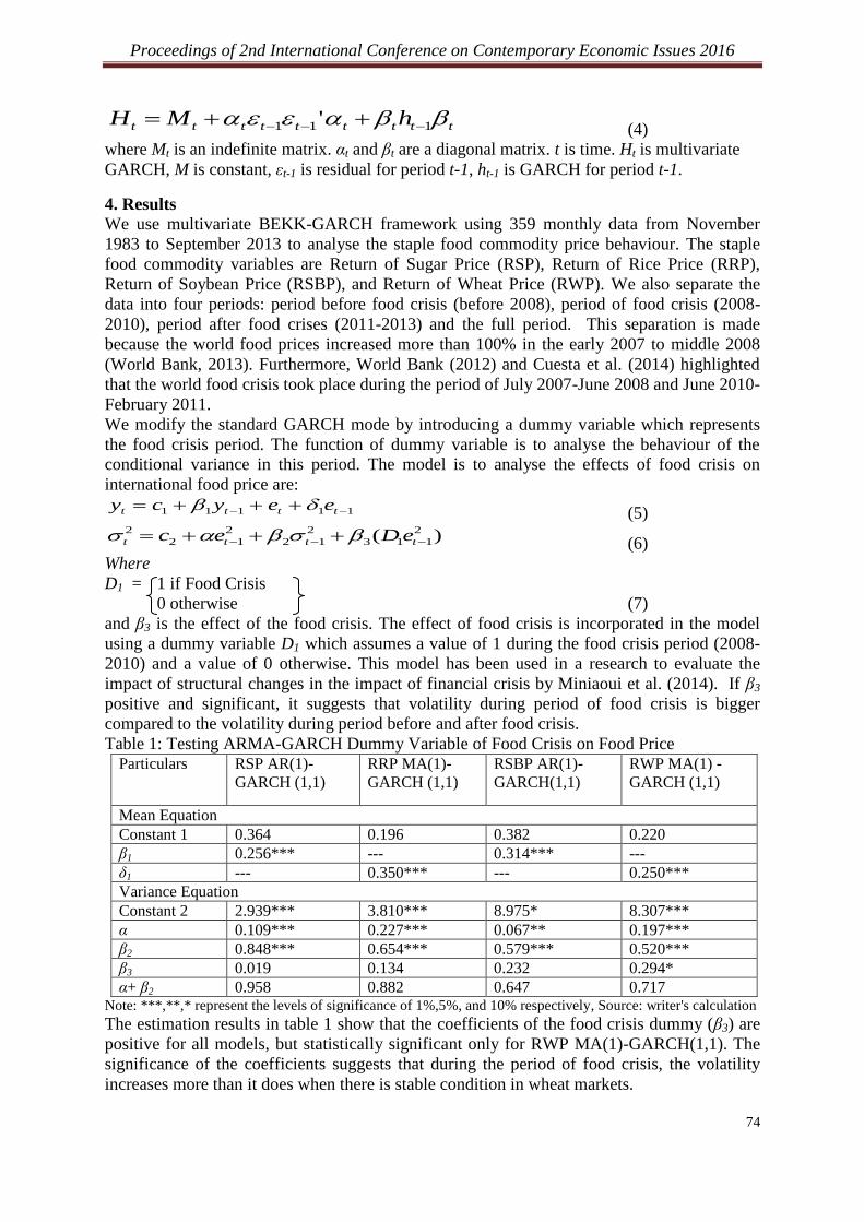
Proceedings of 2nd International Conference on Contemporary Economic Issues 2016
74
ttttttttt hMH 111 ' (4)
where Mt is an indefinite matrix. αt and βt are a diagonal matrix. t is time. Ht is multivariate
GARCH, M is constant, εt-1 is residual for period t-1, ht-1 is GARCH for period t-1.
4. Results
We use multivariate BEKK-GARCH framework using 359 monthly data from November
1983 to September 2013 to analyse the staple food commodity price behaviour. The staple
food commodity variables are Return of Sugar Price (RSP), Return of Rice Price (RRP),
Return of Soybean Price (RSBP), and Return of Wheat Price (RWP). We also separate the
data into four periods: period before food crisis (before 2008), period of food crisis (2008-
2010), period after food crises (2011-2013) and the full period. This separation is made
because the world food prices increased more than 100% in the early 2007 to middle 2008
(World Bank, 2013). Furthermore, World Bank (2012) and Cuesta et al. (2014) highlighted
that the world food crisis took place during the period of July 2007-June 2008 and June 2010-
February 2011.
We modify the standard GARCH mode by introducing a dummy variable which represents
the food crisis period. The function of dummy variable is to analyse the behaviour of the
conditional variance in this period. The model is to analyse the effects of food crisis on
international food price are:
11111 tttt eeycy (5)
)( 2
113
2
12
2
12
2
tttt eDec (6)
Where
D1 = 1 if Food Crisis
0 otherwise (7)
and β3 is the effect of the food crisis. The effect of food crisis is incorporated in the model
using a dummy variable D1 which assumes a value of 1 during the food crisis period (2008-
2010) and a value of 0 otherwise. This model has been used in a research to evaluate the
impact of structural changes in the impact of financial crisis by Miniaoui et al. (2014). If β3
positive and significant, it suggests that volatility during period of food crisis is bigger
compared to the volatility during period before and after food crisis.
Table 1: Testing ARMA-GARCH Dummy Variable of Food Crisis on Food Price Particulars RSP AR(1)-
GARCH (1,1)
RRP MA(1)-
GARCH (1,1)
RSBP AR(1)-
GARCH(1,1)
RWP MA(1) -
GARCH (1,1)
Mean Equation
Constant 1 0.364 0.196 0.382 0.220
β1 0.256*** --- 0.314*** ---
δ1 --- 0.350*** --- 0.250***
Variance Equation
Constant 2 2.939*** 3.810*** 8.975* 8.307***
α 0.109*** 0.227*** 0.067** 0.197***
β2 0.848*** 0.654*** 0.579*** 0.520***
β3 0.019 0.134 0.232 0.294*
α+ β2 0.958 0.882 0.647 0.717 Note: ***,**,* represent the levels of significance of 1%,5%, and 10% respectively, Source: writer's calculation
The estimation results in table 1 show that the coefficients of the food crisis dummy (β3) are
positive for all models, but statistically significant only for RWP MA(1)-GARCH(1,1). The
significance of the coefficients suggests that during the period of food crisis, the volatility
increases more than it does when there is stable condition in wheat markets.

Proceedings of 2nd International Conference on Contemporary Economic Issues 2016
75
We extend the univariate framework to multivariate GARCH model in analysing the own and
cross volatility spillovers between Sugar, Rice, Soybean, and Wheat Prices. We also focused
on the simple model of order (1,1). This order was chosen because it is easier to be
generalized to higher order. The estimated coefficients in this section are assigned as follows:
if the coefficient is βij, for i,j=1,2,3,4, then Return of Sugar Price (RSP) =1, Return of Rice
Price (RRP) =2, Return of Soybean Price (RSBP) = 3, and Return of Wheat Price (RWP) = 4.
Moreover, this part estimates the result for the variance-covariance parameters. The volatility
spillover (transmissions) across international food markets is an interesting topic for investors,
portfolio managers and international traders. If stakeholder can explain the volatility spillover,
then they can make successful hedging and trading strategies (Hernández et al., 2011).
The important contribution in this analysis is that it examines Sugar, Rice, Soybean, and
Wheat Prices simultaneously. The argument is that these four commodities markets are in the
same food basket. According to Schnepf (2013), this food price tends to move together. The
researchers seldom analysed the four markets together.
The multivariate diagonal BEKK-GARCH parameter estimations are summarized in the table
2 for the period before food crisis. The parameters show the impact of αt and βt. In the period
before food crisis, α(1,1), α(2,2), α(3,3) and α(4,4) parameters are significant in all ARMA-
GARCH(1,1) model. α(2,2). β(2,2) and β(4,4) parameters are also significant in all ARMA-
GARCH(1,1) model. β(1,1) parameter is significant in AR(1)-GARCH(1,1) and MA(1)-
GARCH(1,1). β(3,3) is significant in MA(1)-GARCH(1,1) model.
Table 2: Estimated Coefficients for Multivariate Diagonal BEKK- GARCH(1,1)
for RSP, RRP, RSBP, and RWP Period Before Food Crisis Period Parameter ARMA(0,0)
GARCH(1,1)
AR(1)
GARCH(1,1)
MA(1)
GARCH(1,1)
ARMA(1,1)
GARCH(1,1)
Coefficient Coefficient Coefficient Coefficient
Before
Food
Crisis
M(1,1) 7.587*** 6.114*** 6.222*** 7.193***
M(1,2) -0.129 0.097 0.119 0.034
M(1,3) 0.463 0.641* 0.557 0.620
M(1,4) 0.890*** 1.488** 1.434*** 0.974
M(2,2) 0.877* 0.755 0.721 0.716
M(2,3) 1.241 0.463 0.647 0.650
M(2,4) 0.325 0.441 0.582 0.564
M(3,3) 4.554*** 4.435*** 4.149*** 4.334***
M(3,4) 1.879*** 2.438*** 2.705*** 2.652***
M(4,4) 1.824*** 0.002 0.00002 0.000
α(1,1) 0.518*** 0.513*** 0.496*** 0.538**
α(2,2) 0.383*** 0.326*** 0.319*** 0.317***
α(3,3) 0.493*** -0.254** -0.231** -0.240**
α(4,4) 0.415*** -0.253** -0.247** -0.239**
β(1,1) 0.000 0.473*** 0.464*** 0.000
β(2,2) -0.918*** 0.937*** 0.940*** -0.941***
β(3,3) 0.070 0.381 0.496** -0.421
β(4,4) -0.753*** -0.785*** -0.752*** 0.790***
Note: ***,**,* represent the levels of significance of 1%, 5%, and 10% respectively.
1=RSP,2=RRSP, 3=RSBP, 4=RWP, Source: writer's calculation
The own-volatility spillover effect for sugar price is bigger compare to other staple food price.
This condition can be caused by ratoon management harvesting method in sugar cane. Most
of the sugar cane harvest is using ratooning method which leaves the roots, the lower parts of
sugar cane uncut and can be harvested again more than ten times (Latief et al., 2010). This
method is not applied in other staple food except for a relatively small amount of rice. The
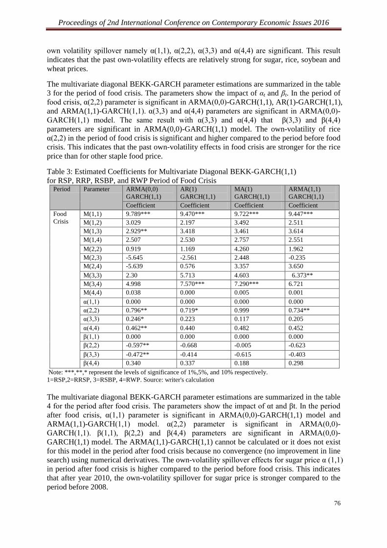
Proceedings of 2nd International Conference on Contemporary Economic Issues 2016
76
own volatility spillover namely α(1,1), α(2,2), α(3,3) and α(4,4) are significant. This result
indicates that the past own-volatility effects are relatively strong for sugar, rice, soybean and
wheat prices.
The multivariate diagonal BEKK-GARCH parameter estimations are summarized in the table
3 for the period of food crisis. The parameters show the impact of αt and βt. In the period of
food crisis, α(2,2) parameter is significant in ARMA(0,0)-GARCH(1,1), AR(1)-GARCH(1,1),
and ARMA(1,1)-GARCH(1,1). α(3,3) and α(4,4) parameters are significant in ARMA(0,0)-
GARCH(1,1) model. The same result with α(3,3) and α(4,4) that β(3,3) and β(4,4)
parameters are significant in ARMA(0,0)-GARCH(1,1) model. The own-volatility of rice
α(2,2) in the period of food crisis is significant and higher compared to the period before food
crisis. This indicates that the past own-volatility effects in food crisis are stronger for the rice
price than for other staple food price.
Table 3: Estimated Coefficients for Multivariate Diagonal BEKK-GARCH(1,1)
for RSP, RRP, RSBP, and RWP Period of Food Crisis Period Parameter ARMA(0,0)
GARCH(1,1)
AR(1)
GARCH(1,1)
MA(1)
GARCH(1,1)
ARMA(1,1)
GARCH(1,1)
Coefficient Coefficient Coefficient Coefficient
Food
Crisis
M(1,1) 9.789*** 9.470*** 9.722*** 9.447***
M(1,2) 3.029 2.197 3.492 2.511
M(1,3) 2.929** 3.418 3.461 3.614
M(1,4) 2.507 2.530 2.757 2.551
M(2,2) 0.919 1.169 4.260 1.962
M(2,3) -5.645 -2.561 2.448 -0.235
M(2,4) -5.639 0.576 3.357 3.650
M(3,3) 2.30 5.713 4.603 6.373**
M(3,4) 4.998 7.570*** 7.290*** 6.721
M(4,4) 0.038 0.000 0.005 0.001
α(1,1) 0.000 0.000 0.000 0.000
α(2,2) 0.796** 0.719* 0.999 0.734**
α(3,3) 0.246* 0.223 0.117 0.205
α(4,4) 0.462** 0.440 0.482 0.452
β(1,1) 0.000 0.000 0.000 0.000
β(2,2) -0.597** -0.668 -0.005 -0.623
β(3,3) -0.472** -0.414 -0.615 -0.403
β(4,4) 0.340 0.337 0.188 0.298
Note: ***,**,* represent the levels of significance of 1%,5%, and 10% respectively.
1=RSP,2=RRSP, 3=RSBP, 4=RWP. Source: writer's calculation
The multivariate diagonal BEKK-GARCH parameter estimations are summarized in the table
4 for the period after food crisis. The parameters show the impact of αt and βt. In the period
after food crisis, α(1,1) parameter is significant in ARMA(0,0)-GARCH(1,1) model and
ARMA(1,1)-GARCH(1,1) model. α(2,2) parameter is significant in ARMA(0,0)-
GARCH(1,1). β(1,1), β(2,2) and β(4,4) parameters are significant in ARMA(0,0)-
GARCH(1,1) model. The ARMA(1,1)-GARCH(1,1) cannot be calculated or it does not exist
for this model in the period after food crisis because no convergence (no improvement in line
search) using numerical derivatives. The own-volatility spillover effects for sugar price α (1,1)
in period after food crisis is higher compared to the period before food crisis. This indicates
that after year 2010, the own-volatility spillover for sugar price is stronger compared to the
period before 2008.
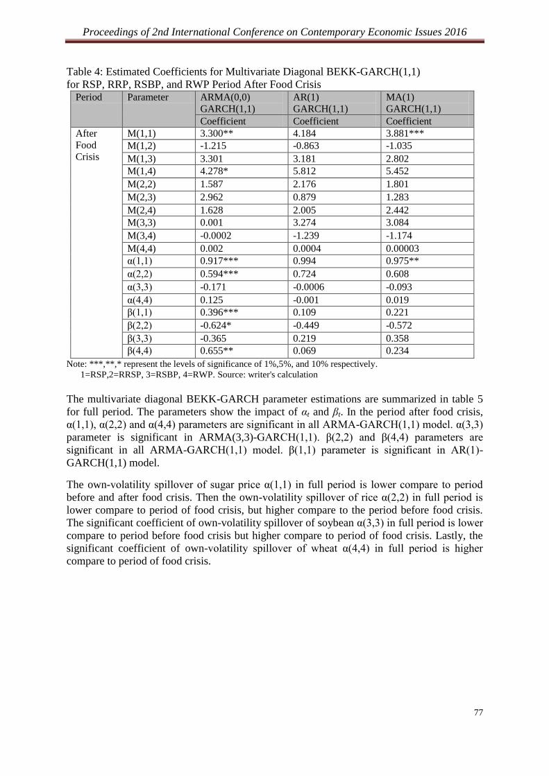
Proceedings of 2nd International Conference on Contemporary Economic Issues 2016
77
Table 4: Estimated Coefficients for Multivariate Diagonal BEKK-GARCH(1,1)
for RSP, RRP, RSBP, and RWP Period After Food Crisis Period Parameter ARMA(0,0)
GARCH(1,1)
AR(1)
GARCH(1,1)
MA(1)
GARCH(1,1)
Coefficient Coefficient Coefficient
After
Food
Crisis
M(1,1) 3.300** 4.184 3.881***
M(1,2) -1.215 -0.863 -1.035
M(1,3) 3.301 3.181 2.802
M(1,4) 4.278* 5.812 5.452
M(2,2) 1.587 2.176 1.801
M(2,3) 2.962 0.879 1.283
M(2,4) 1.628 2.005 2.442
M(3,3) 0.001 3.274 3.084
M(3,4) -0.0002 -1.239 -1.174
M(4,4) 0.002 0.0004 0.00003
α(1,1) 0.917*** 0.994 0.975**
α(2,2) 0.594*** 0.724 0.608
α(3,3) -0.171 -0.0006 -0.093
α(4,4) 0.125 -0.001 0.019
β(1,1) 0.396*** 0.109 0.221
β(2,2) -0.624* -0.449 -0.572
β(3,3) -0.365 0.219 0.358
β(4,4) 0.655** 0.069 0.234
Note: ***,**,* represent the levels of significance of 1%,5%, and 10% respectively.
1=RSP,2=RRSP, 3=RSBP, 4=RWP. Source: writer's calculation
The multivariate diagonal BEKK-GARCH parameter estimations are summarized in table 5
for full period. The parameters show the impact of αt and βt. In the period after food crisis,
α(1,1), α(2,2) and α(4,4) parameters are significant in all ARMA-GARCH(1,1) model. α(3,3)
parameter is significant in ARMA(3,3)-GARCH(1,1). β(2,2) and β(4,4) parameters are
significant in all ARMA-GARCH(1,1) model. β(1,1) parameter is significant in AR(1)-
GARCH(1,1) model.
The own-volatility spillover of sugar price α(1,1) in full period is lower compare to period
before and after food crisis. Then the own-volatility spillover of rice α(2,2) in full period is
lower compare to period of food crisis, but higher compare to the period before food crisis.
The significant coefficient of own-volatility spillover of soybean α(3,3) in full period is lower
compare to period before food crisis but higher compare to period of food crisis. Lastly, the
significant coefficient of own-volatility spillover of wheat α(4,4) in full period is higher
compare to period of food crisis.
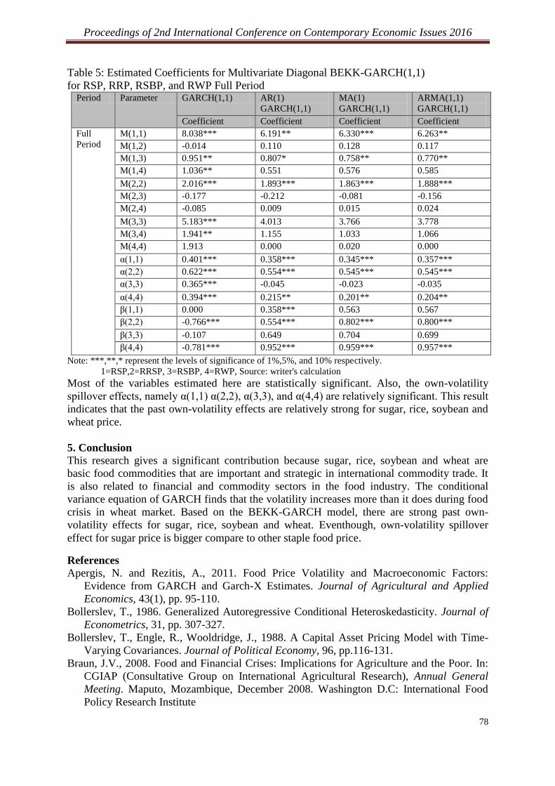
Proceedings of 2nd International Conference on Contemporary Economic Issues 2016
78
Table 5: Estimated Coefficients for Multivariate Diagonal BEKK-GARCH(1,1)
for RSP, RRP, RSBP, and RWP Full Period Period Parameter GARCH(1,1) AR(1)
GARCH(1,1)
MA(1)
GARCH(1,1)
ARMA(1,1)
GARCH(1,1)
Coefficient Coefficient Coefficient Coefficient
Full
Period
M(1,1) 8.038*** 6.191** 6.330*** 6.263**
M(1,2) -0.014 0.110 0.128 0.117
M(1,3) 0.951** 0.807* 0.758** 0.770**
M(1,4) 1.036** 0.551 0.576 0.585
M(2,2) 2.016*** 1.893*** 1.863*** 1.888***
M(2,3) -0.177 -0.212 -0.081 -0.156
M(2,4) -0.085 0.009 0.015 0.024
M(3,3) 5.183*** 4.013 3.766 3.778
M(3,4) 1.941** 1.155 1.033 1.066
M(4,4) 1.913 0.000 0.020 0.000
α(1,1) 0.401*** 0.358*** 0.345*** 0.357***
α(2,2) 0.622*** 0.554*** 0.545*** 0.545***
α(3,3) 0.365*** -0.045 -0.023 -0.035
α(4,4) 0.394*** 0.215** 0.201** 0.204**
β(1,1) 0.000 0.358*** 0.563 0.567
β(2,2) -0.766*** 0.554*** 0.802*** 0.800***
β(3,3) -0.107 0.649 0.704 0.699
β(4,4) -0.781*** 0.952*** 0.959*** 0.957***
Note: ***,**,* represent the levels of significance of 1%,5%, and 10% respectively.
1=RSP,2=RRSP, 3=RSBP, 4=RWP, Source: writer's calculation
Most of the variables estimated here are statistically significant. Also, the own-volatility
spillover effects, namely α(1,1) α(2,2), α(3,3), and α(4,4) are relatively significant. This result
indicates that the past own-volatility effects are relatively strong for sugar, rice, soybean and
wheat price.
5. Conclusion
This research gives a significant contribution because sugar, rice, soybean and wheat are
basic food commodities that are important and strategic in international commodity trade. It
is also related to financial and commodity sectors in the food industry. The conditional
variance equation of GARCH finds that the volatility increases more than it does during food
crisis in wheat market. Based on the BEKK-GARCH model, there are strong past own-
volatility effects for sugar, rice, soybean and wheat. Eventhough, own-volatility spillover
effect for sugar price is bigger compare to other staple food price.
References
Apergis, N. and Rezitis, A., 2011. Food Price Volatility and Macroeconomic Factors:
Evidence from GARCH and Garch-X Estimates. Journal of Agricultural and Applied
Economics, 43(1), pp. 95-110.
Bollerslev, T., 1986. Generalized Autoregressive Conditional Heteroskedasticity. Journal of
Econometrics, 31, pp. 307-327.
Bollerslev, T., Engle, R., Wooldridge, J., 1988. A Capital Asset Pricing Model with Time-
Varying Covariances. Journal of Political Economy, 96, pp.116-131.
Braun, J.V., 2008. Food and Financial Crises: Implications for Agriculture and the Poor. In:
CGIAP (Consultative Group on International Agricultural Research), Annual General
Meeting. Maputo, Mozambique, December 2008. Washington D.C: International Food
Policy Research Institute
Proceedings of 2nd International Conference on Contemporary Economic Issues 2016
79
Briesch, R.A., Krishnamurthi, L, Mazumdar, T. and Raj, S.P., 1997. A Comparative Analysis
of Reference Price Models. Journal of Consumer Research, 24, September.
Cuesta, J., Htenas, A. and Tiwari, S., 2014. Monitoring Global and National Food Price
Crisis. Food Policy, 49, pp. 84-94.
Engle, R. and Kroner, K., 1995. Multivariate Simultaneous GARCH. Econometric Theory 11,
pp. 122-150.
FAO, 2011. The State of Food Insecurity in the World. Rome: Food and Agriculture
Organization of the United Nations.
Hernández, M.A., Ibarra-Ramírez, R. and Trupkin, D.R., 2011. How Far Do Shocks Move
Across Borders? Examining Volatility Transmission in Major Agricultural Futures
Markets. Banco de México Working Paper N 2011-15. Mexico: Banco de México
IMF, 2008. Financial Stress and Deleveraging Macrofinancial Implications and Policy.
Washington D.C: International Monetary Fund.
Lahiani, A., Nguyen, D. K. and Vo, T., 2014. Understanding Return and Volatility Spillovers
among Major Agricultural Commodities. Institut de Préparation à l'Administration et à la
Gestion Business School Working Paper 2014-243. Paris: IPAG.
Latief, A. S., Syarief, R., Pramudya, B. and Muhadiono, 2010. Productivity of Sugarcane
Plants of Ratooning with Fertilizing Treatment. Nusantara Bioscience, 2 (1), pp.43-47.
Mahon, C., 2012. The Right to Food: A Right for Everyone. In C. Rosin, P. Stock and H.
Campbell (eds), Food Systems Failure: The Global Food Crisis and The Future of
Agriculture. London: Oxon.
Miniaoui, H., Sayani, H. and Chaibi, A., 2014. The Impact of Financial Crisis on Islamic and
Conventional Indices of the GCC Countries. Institut de Préparation à l'Administration et à
la Gestion Business School Working Paper 2014-401. Paris: IPAG.
Naylor, R.L. and Falcon, W.P., 2010. Food Security in an Era of Economic Volatility.
Population and Development Review, 36 (4), pp. 693-723.
Schnepf, R., 2013. Consumers and Food Price Inflation. Washington D.C: Congressional
Research Service.
Serra, T., Zilberman, D., Gil, J.M., and Goodwin, B.K., 2011. Nonlinearities in the US Corn-
Ethanol-Oil-Gasoline Price System. Agricultural Economics, 42 (1), pp. 35-45.
World Bank, 2012. The Food Price Crisis Monitor. Report of World Bank. [online] Available
through: <http://www.worldbank.org/content/dam/Worldbank/
document/Poverty%20documents/Introduction%20
Guide%20for%20the%20Crisis%20Monitor.pdf>. [Accessed 25 November 2014].
World Bank, 2013. The World Bank Group and the Global Food Crisis: An Evaluation of the
World Bank Group Response, Report. Wassington D.C: World Bank Group.
Worthington, A. and Higgs, H., 2004. Transmission of Equity Returns and Volatility in Asian
Developed and Emerging Markets: A Multivariate GARCH Analysis. International
Journal of Finance and Economics, 9 (1), pp.71-80.
Wu, H. and Li, S., 2013. Volatility Spillovers in China’s Crude Oil, Corn and Fuel Ethanol
Markets. Energy Policy, 62, pp. 878-886.
Zhang, Z. Lohr, L., Escalante, C. and Wetzstein, M., 2010. Food Versus Fuel: What Do Price
Tell US? Energy Policy, 38, pp. 445-451.

Proceedings of 2nd International Conference on Contemporary Economic Issues 2016
80
LIST OF AUTHORS
Abdul Fatah Che Hamat
Abdul Rahim Ridzuan
Chee-Hong Law
Dzul Hadzwan Husaini
Ee Shiang Lim
Geok Peng Yeap
Ghee-Thean Lim
Hooi Hooi Lean
Jacqueline Liza Fernandez
Jerome Kueh
Kumara Jati Gamini Premaratne
Muhammad Asraf Abdullah
Muzafar Shah Habibullah
Nor Asmat Ismail
Sakkarin Nonthapot
Sotheeswari Somasundram
Sze-Wei Yong
Venus Khim-Sen Liew

Proceedings of 2nd International Conference on Contemporary Economic Issues 2016
81
LIST OF REVIEWERS
Andrew K.G. Tan
Chee-Hong Law
Chee Lip Tee
Chor Foon Tang
Ee Shiang Lim
Ghee-Thean Lim
Kar Yee Ng
Mohd Taufik bin Mohammad
Nor Asmat Ismail
Nurul Huda Mohd Satar
Parthiban S.Gopal
Premalatha Karupiah
Radin Firdaus Radin Badaruddin
Radziah Adam
Selamah Maamor
Siti Aisyah Baharudin
Siti Rahyla Rahmat
Soo Yean Chua
Pei Sung Toh
Tze-Haw Chan
Tze San Ong
Yiing Jia Loke