proceedings - 情報科学研究科 | naist...

Proceedings

International Workshop on

Empirical Software Engineering in Practice 2010

(IWESEP 2010)

Nara, Japan, December 7-8, 2010

Sponsored by StagE Project, MEXT Japan

Foundation for Nara Institute of Science and Technology Microsoft Research Osaka University

Nara Institute of Science and Technology (NAIST)

In cooperation with SIG Software Science, Information and Systems Society, IEICE

SIG Software Engineering, IPSJ

Table of Contents Preface ............................................................................................................................ ivOrganization .................................................................................................................. vi

Keynote Address Empirical Software Engineering and Measurement at Microsoft ..................................... 3

Thomas Zimmermann

Project Management Process Fragment Based Process Complexity with Workflow Management Tables ........ 7

Masaki Obana, Noriko Hanakawa, Norihiro Yoshida and Hajimu Iida

Applying Outlier Deletion to Analogy Based Cost Estimation ....................................... 13 Masateru Tsunoda, Akito Monden, Mizuho Watanabe,

Takeshi Kakimoto and Ken-ichi Matsumoto

A Survey of Public Datasets for Comparative Effort Prediction Studies ........................ 19 Sousuke Amasaki and Tomoyuki Yokogawa

Faults and Verification Reconstructing Fine-Grained Versioning Repositories with Git for Method-Level Bug Prediction ............................................................................. 27 Hideaki Hata, Osamu Mizuno and Tohru Kikuno

Reachability Analysis of Probabilistic Timed Automata Based on an Abstraction Refinement Technique ............................................................ 33 Takeshi Nagaoka, Akihiko Ito, Toshiaki Tanaka, Kozo Okano and Shinji Kusumoto

Fault-prone Module Prediction Using Contents of Comment Lines ............................... 39 Osamu Mizuno and Yukinao Hirata

ii

Process Analysis A Preliminary Study on Impact of Software Licenses on Copy-and-Paste Reuse .......... 47 Yu Kashima, Yasuhiro Hayase, Norihiro Yoshida, Yuki Manabe and Katsuro Inoue

Using Program Slicing Metrics for the Analysis of Code Change Processes ................. 53 Raula Gaikovina Kula, Kyohei Fushida, Norihiro Yoshida and Hajimu Iida

Flexibly Highlighting in Replaying Operation History ................................................... 59 Takayuki Omori and Katsuhisa Maruyama

iii

Preface

It is our great pleasure to welcome everyone to the International Workshop on Empirical Software Engineering in Practice 2010 (IWESEP 2010). Our workshop is to foster the development of the area by providing a forum where young researchers and practitioners can report on and discuss their new research results and applications in the area of empirical software engineering. The workshop encourages the exchange of ideas within the international community so as to be able to understand, from an empirical viewpoint, strengths and weaknesses of technology in use and new technologies, with the expectation of furthering the more generic field of software engineering.

IWESEP has received 13 submission including 12 regular papers and 1 tool demonstration proposal. After the careful evaluations of the program committee, 8 regular papers and 1 tool demonstration have been accepted to be presented at the workshop. The papers cover a variety of topics, including project management, fault prediction, formal verification and analysis of software development process. In addition, the program includes a keynote speech by Dr. Thomas Zimmermann. We hope that these proceedings will serve as a valuable reference for researchers and developers.

In addition, we hold the MSR School in Asia as the tutorial at IWESEP 2010. The MSR School in Asia provides an overview of the Mining Software Repositories (MSR) filed and an opportunity to learn the techniques used in this field. MSR is a rapidly growing field that holds an annual tutorial and a co-located working conference at the International Conference on Software Engineering (ICSE) every year. We have invited some of the top researchers, Dr. Ahmed Hassan, Dr. Sunghun Kim, and Dr. Thomas Zimmermann, in the MSR field to give the tutorial.

Finally, on behalf of the program committee and the organizing committee, we thank you for attending IWESEP 2010 and hope that you will we enjoy the workshop. We would like to take this opportunity to thank the organizers who spend considerable time reviewing publications and preparations for this workshop.

iv

We hope you will have a great time and an unforgettable experience at the IWESEP2010.

Akinori Ihara, Nara Institute of Science and Technology, Japan IWESEP 2010 General Chair

Takashi Ishio, Osaka University, Japan IWESEP2010 Program Chair

v

Organization

General Chair Akinori Ihara (Nara Institute of Science and Technology, Japan)

Program Chair Takashi Ishio (Osaka University, Japan)

Publication Chair Kyohei Fushida (Nara Institute of Science and Technology, Japan)

Publicity Co-Chair Sunghun Kim (Hong Kong University of Science and Technology, China) Masataka Nagura (Hitachi, Ltd., Japan) Emad Shihab (Queen’s University, Canada)

Registration Chair Masateru Tsunoda (Nara Institute of Science and Technology, Japan)

Local Arrangements Chair Norihiro Yoshida (Nara Institute of Science and Technology, Japan)

vi

Program Committee Bram Adams (Queen’s University, Canada) Sousuke Amasaki (Okayama Prefectural University, Japan) Christian Bird (Microsoft Research, USA) Ahmed E. Hassan (Queen’s University, Canada) Hideaki Hata (Osaka University, Japan) Shinpei Hayashi (Tokyo Institute of Technology, Japan) Israel Herraiz (University Alfonso X el Sabio, Spain) Yasutaka Kamei (Queen’s University, Canada) Masa Katahira (JAXA, Japan) Shinji Kawaguchi (JAMSS, Japan) Jacky Keung (NICTA, Australia) Hua Jie Lee (University of Melbourne, Australia) Shinsuke Matsumoto (Kobe University, Japan) Koji Toda (Nara Institute of Science and Technology, Japan) Hidetake Uwano (Nara National College of Technology, Japan) Rodrigo Vivanco (University of Manitoba, Canada) Thomas Zimmermann (Microsoft Research, USA)

vii

Keynote Address

1

Keynote AddressEmpirical Software Engineering and Measurement at Microsoft

Thomas Zimmermann (Microsoft Research / University of Calgary)

Abstract:Software engineering is an data rich activity: changes to source code are recorded in version archives, bugs are reported to issue tracking systems, and communications are archived in e-mails and newsgroups. The Empirical Software Engineering and Measurement (ESM) group at Microsoft Research analyzes such data to better understand various software development issues from an empirical perspective. In this talk, I will highlight our research themes and activities using examples from our research on socio technical congruence, bug reporting and triaging, and data-driven software engineering. I will highlight our unique ability to leverage industrial data and developers and the ability to make near term impact on Microsoft via the results of our studies. The work presented in this talk has been done by Chris Bird, Brendan Murphy, Nachi Nagappan, myself, and many others who have visited our group over the past years.

3

Project Management

5

Process Fragment Based Process Complexity with Workflow Management Tables

Masaki Obana1 , Noriko Hanakawa2 , Norihiro Yoshida1 , Hajimu Iida1 1Nara Institute Science and Technology

2Hannan University

[email protected], [email protected], [email protected], [email protected]

ABSTRACT The actual software development processes deviate from initial model planned at early stage. One of the reasons is that additional processes get triggered by urgent changes of software specifications. Such additional processes increase the complexity of the whole development process, and possibly decrease the product quality. In this paper, we propose a novel complexity measure of software process, which based on the number of process fragments, the number of simultaneous process fragments, and the number of developers’ groups. Proposed process complexity is applied to two industrial projects in order to show the usefulness of this measure. As a result, we found that the higher value of process complexity indicates higher risk of products' faults.

Categories and Subject Descriptors D.2.9 [Software Engineering]: Management: software process models

General Terms Management, Measurement.

Keywords Process complexity, risk management, a workflow management table, change of customers’ demand.

1. Introduction In software development projects, large gaps between planned development processes and actual executed development processes exist. Even if a development team has originally selected the waterfall model unplanned small processes are often triggered as shown in the following examples.

i. One activity of waterfall-based process is changed into new iterative process because of urgent specification changes.

ii. Developers design GUI using a new prototype development process at design phase.

iii. In an incremental development process, developers correct defects in the previous release while developers are implementing new functions in current release.

That is, the waterfall-based process at planning time is often gradually transformed into the combination of the original waterfall-based process and several unplanned small processes (hereinafter referred to as process fragments). In consequence, actual development processes are more complicated than planned one (see also Figure 1).

In this paper, we firstly assume that complicated process decreases product quality, and then propose a new metric for

process complexity based on the number of unplanned process fragments, the number of simultaneous execution processes, and the number of developers' groups. It can be used to visualize how process complexity increases as actual development process proceeds.

An aim of measuring process complexity is to prevent software from becoming low quality product. A process complexity is derived from a base process and process fragments. A base process means an original process that was planned at the beginning of a project. Process fragments mean additional and piecemeal processes that are added to the base process on the way of a project. Process fragment occurs by urgent changes of customers’ requirement, or sudden occurrence of debugging faults. Process fragments can be extracted from actual workflow management tables which are popular in Japanese industrial projects. We especially focus on simultaneous execution of multiple processes to model the process complexity. Simultaneous execution of multiple processes is caused by adding process fragments on the way of a project. Finally, we perform an industrial case study in order to show the usefulness of process complexity. In this case study, we found that process complexity indicated the degree of risk of post-release faults.

Section 2 shows related work about process metrics, and risk management. The process complexity is proposed in section 3. Section 3 also describes how the proposed complexity would be used in industrial projects. Case studies of two projects are shown in section 4. In section 5, we discuss a way of risk management using the process complexity. Summary and future works are described in Section 6.

2. Related Work Many software development process measurement techniques have been proposed. CMM [1] is a process maturity model by Humphrey. Five maturity levels of organizations have been proposed in CMM. When a maturity level is determined, various values of parameters (faults rate in total test, test density, review density) are collected. In addition, Sakamoto et al. proposed a metrics for measuring process improvement levels [2]. The metrics were applied to a project based on a waterfall process model. Theses process measurement metrics’ parameters include the number of times of review execution and the number of faults in the reviewed documents. The aim of these process measurement techniques is improvement of process maturity of an organization, while our research aims to measure process complexity of a project, not organization. Especially, changes of process complexity in a project clearly are presented by our process complexity.

7

Many researches of process modeling techniques have been ever proposed. Cugola et al. proposed a process modeling language that describes easily additional tasks [3]. Extra tasks are easily added to a normal development process model using the modeling language. Fuggetta et al. proposed investigated problems about software development environments and tools oriented on various process models [4]. These process modeling techniques are useful to simulate process models in order to manage projects. However, these process modeling techniques make no mention of process complexity in a project.

In a field of industrial practices, Rational Unified Process (RUP) has been proposed [5]. The RUP has evolved in integrating several practical development processes. The RUP includes Spiral process model, use-case oriented process model, and risk oriented process model. Moreover, the RUP can correspond to the latest development techniques such as agile software development, and .NET framework development. Although problems of management and scalability exist, the RUP is an efficient integrated process for practical fields. The concept of the various processes integration is similar to our process fragments integration, while the RUP is a pre-planned integration processes. The concept of our process complexity is based on more flexible model considering changes of development processes during a project execution. Our process complexity focuses on changes of an original development process by process fragments, and regarded as a development processes change.

Garcia et al. evaluated maintainability and modifiability of process models using new metrics based on GQM [6]. They focus on additional task as modifiability. The focus of additional task is similar to our concept of process complexity. Although their research target is theoretical process models, and our research target is practical development processes. In this way , there was no studies for measuring complexity of process during a project as long as we examined it. Therefore, the originality of our proposed complexity may be high.

3. Proposed Metrics Based on Process fragment 3.1 Process fragment In software development, a manager makes a plan of a single development process like a waterfall process model at the beginning of a project. However, the planned single process usually continues to change until the end of the project. For example, at the beginning of a project, a manager makes a plan based on a waterfall process model. However the original process is changed to an incremental process model because several functions’ development is shifted to next version’s development. Moreover, at the requirement analysis phase, prototyping process may be added to an original process in order to satisfy customers’ demands. If multiple releases like an incremental process model exist, developers have to implement new functions while developers correct detects that were caused in the previous version’s development. In this paper, we call the original process “a base process”, we call the additional process “a process fragment”. While original process is a process that was planned at the beginning of a project, a process fragment is a process that is added to the original process on the way of a project. �Fragment” means piecemeal process. Process fragments are simultaneously executed with a base process. Process fragment

does not mean simple refinement of a base process, but rather may separately executes from a base process execution.

Figure1 shows an example of process fragment. At the planning phase, it is a simple development process that consists of analysis activity, design activity, implementation activity, and testing activity. In many cases, because of insufficient information, a manager often makes a rough simple process (macro process) rather than a detailed process (micro process) [7]. However, information about software increases as a project progresses, and the original simple process changes to more complicated processes. In the case of Figure 1, at the analysis phase, an unplanned prototype process was added to the original process because of customers’ requests. As a result of analysis phase, implementations of some functions were shifted to next version development because of constraints of resources such as time, cost, and human. The process fragments were shown at the Figure1 as small black boxes. In the design phase, because customers detected miss-definitions of system specifications that were determined in the previous analysis phase, a process for reworking of requirement analysis was added to the development process. Moreover, the manager shifted the development of a combination function with the outside system when the outside system was completed. During the implementation phase, several reworks of designs occurred. In the test phase, reworks of designs occurred because of low performance of several functions.

Analysis Design Implement Test A base Process

A part of function is next version.

Process fragments

The re-design, the re-implement, and the re-test are executed for the performance improvement.

A part of function is developed by the prototype.

A fragment process

Re-design by requirement definition mistake.

A coordinated design with other systems is executed. later.

Process fragments

Analysis Design Implement Test



Process fragments

Figure 1 A concept of process fragments

Plan phase

Analysis phase

Design phase

Implement

phase

A part of function to the next version for the delivery date.


A part of function is re-designed and re-implemented by the requirement definition mistake.

Process fragments

Test phase

8

Process fragments are caused by urgent customers’ requests, design errors, combination with outside systems on the way of development. Various sizes of process fragments exist. A small process fragment includes only an action such as document revision. A large process fragment may include more activities for example, a series of developing activities; design activity, implementation activity, and test activity.

3.2 Calculation of process complexity 3.2.1 Extracting process fragments Process complexity is calculated based on process fragments. Process fragments are identified from a series of workflow management table. That is a continuator revised along the project. Figure 2 shows two versions of a workflow management table. Each column means a date, each row means an activity. A series of A, B, C activities is a base process. D, E, F activities are added to the base process on May 1. Therefore, D, E, F activities are process fragments. On Jun. 1, the base process and three process fragments are simultaneously executed. In this way, process fragments can be identified from configuration management of a workflow management table. Difference between current version and previous version of a workflow management table means process fragments. Of course, the proposed complexity is available in various development processes such as an agile process as long as managers manage process fragments in various management charts.

3.2.2 Definition of process complexity Process complexity is defined by the following equation.

��

��)(

1)()()()( )_(

tN

iitititt termLdevNumPC

…..(1) PC(t): process complexity on time t N(t): the total number of process on time t Num_dev(t)i: the number of group of developers of the i-th process

fragment on time t L(t)i: the number of simultaneous processes of the i-th process fragment

on time t. But the i-th fragment is eliminated from these multiplications in L(t).

term(t)i: ratio of an executing period of the i-th process fragment for the whole period of the project on time t, that is, if term(t)i is near 1, a executing period of the process fragment is near the whole period of the project.

Basically, proposed process complexity is the accumulation of all process fragments including finished processes. The reason of the accumulation is that the proposed complexity’s target is a whole project, not a spot timing of a project. For example, many process fragments occur at the first half of a project. Even if the process

fragments have finished, the fragments’ executions may harmfully influence products and process at the latter half of the project. Therefore, the proposed complexity is accumulation of all process fragments.

The process complexity basically depends on three elements; the number of group of the i-th process fragment on time t: Num_dev(t)i, the number of simultaneous processes of the i-th process fragment on time t: L(t)i, and ratio of an executing period of the i-th process fragment for the whole period of project time t: term(t)i. Granularity of group of developer(Num_dev(t)i) depends on the scale of process fragments. If a process fragment is in detail of every hour, a group simply correspond to a person. If process fragment is large such as design phase, a group unit will be an organization such as SE group and programmer group. The group of developers will be carefully discussed in future research. The ratio of an executing period of the i-th process fragment for the whole period of project time t (term(t)i) means impact scale of a process fragment. If a process fragment is very large, for example an executing period of the process fragment is almost same as the whole period of a project, the process fragment will influence largely the project. In contrast, if a process fragment is very small, for example an executing period is only one day, the process fragment will not influence a project so much.

In short, when more and larger scale process fragments are simultaneously executed, a value of process complexity becomes larger. When fewer and smaller scale process fragments simultaneously are executed, a value of process complexity becomes smaller. Values of the parameters of equation� (1) are easily extracted from configuration management data of a workflow management table.

3.3 Setting a base process and extracting process fragments At the beginning of a project, a base process is determined. If a planned schedule is based on a typical waterfall process model such as the base process in Figure 1, the parameters’ values of process complexity are t=0, N(�)=1, Num_dev (�)=3 (SE group developer group, customer group), L(� )=1, and term (� )=1. Therefore the value of process complexity PC(0) =3.

As a project progresses, unplanned process fragments are occasionally added to the base process at time t1. A manager registers the process fragments as new activities to the workflow management table. The manager also assigns developers to the new activities. Here, we assume that the planned period of a base process is 180 days. A manager adds two activities to the workflow management table. The period of each additional activity is planned as 10 days. Therefore the total number of process N (t1) = 3, and the process complexity is calculated as follows; (1) for i = 1 (a base process)

� Num_dev(t1) = 3 � L(t1)1 = 3 � term(t1)1 = 180/180 = 1.0

(2) for i = 2 (the first process fragment ) � Num_dev(t1)2 = 1 � L(t1)2= 3 � term(t1)2 = 10/180 = 0.056

(3) for i = 3 (the second process fragment ) � Num_dev(t1)3 = 1 � L(t1)3 = 3 � term(t1)3= 10/180 = 0.056

A

B

C

D

E

F

current

Activity Apr.1 May 1 Jun.1 Jul.1

A

B

C

current

A table on Apr. 1 A table on Jun. 1

Added on May 1

Figure 2 Extracting process fragments from configuration of a workflow management table

Base process

Activity Apr.1 May 1 Jun.1 Jul.1

9

Finally, a value of process complexity at t=t1 can be calculated as PC(t1) = 9.000 +0.168+ 0.168 = 9.336.

In this way, the value of PC(t) at any value of time t can be calculated based on workflow management table.

4. Application to Two Industrial Projects The process complexity has been applied to two practical projects.

4.1 The HInT project The first project’s name is HInT (Hannan Internet communication Tool). The HInT project developed a web-based educational portal system. The development began from October 2007, the release of the HInT was April 2008. Because the workflow management table was updated every week, 20 versions of the workflow management table are obtained. At the beginning of the project, the number of activities in the workflow table was 20. At the end of the project, the number of activities reached to 123. Each activity had a planned schedule and a practice result of execution. Figure 3 shows a rough variation of development process of the project. At the beginning of the project, the shape of the development process was completely a waterfall process. However, at the UI design phase, a prototype process was added to the waterfall process. In the prototype process, four trial versions were presented to customers. At the combination test phase, developers and customers found significant errors of specifications and two process fragments were added to the development process in haste. Reworks such as re-design, re-implement, and re-test for the specification errors continued until the operation test phase. At the system test phase, an error of a function connecting with an outside system occurred and a new process fragment was introduced to the development process. The introduced process fragment consists of various activities such as investigating network environments, investigating specification of the outside system, and revising the programs. These activities continued until the delivery timing. Figure 4 shows process complexity of the HInT project. At the beginning of the project, the value of process complexity was very low while the value of the process complexity increased as the project progresses. In particular, after the system test phase, four processes were simultaneously executed. Then process complexity increased to 44.167.

4.2 The p-HInT project The p-HInT is a lecture support system for large-scale lectures with mobile terminals [8][9]. A base process of the p-HInT project was an incremental development process. We released the p-HInT product four times from April 2008 through April 2010. A development process of the each release included analysis phase, design phase, implement phase, and test phase. At the first version development, basic functions and infrastructure implementation were planned in detail. However, the manager determined only rough design of next versions’ functions. At the second version development, new four functions were developed while the developers fixed defects that had been introduced at the previous version’s development. Of course, the debugging works were not planned in the original schedule. At the third version development, product refactoring was executed because the design of the product became too complicated for introduction of new functions and also for debugging works. At the fourth version development, customers requested new functions that were not discussed at the requirement analysis phase. The customers said that the requested new functions were more important than the functions that were originally planned at the beginning of the project. At same time, performance improvement work for some functions in the previous releases was made at the fourth version development.

Kick off Requirement analysis UI design Programming Combination test System test Operations test Process1

Process1 November

PrototypeProcess2 Four functions are made by the prototype.

Analysis Design Programming Test Process3

Process4Two functions were redeveloped.

Process5The connect functions redeveloped.

Time

Kick off Requirement analysis UI design Programming

Process1 PrototypeProcess2


Analysis Design Programming Test

January

Analysis Design Programming Test Process3

Process4

Process1 PrototypeProcess2



February


Figure 3 A variation of development process of the HInT project

October

Combination test System test Operations test



Figure 4 Process complexity of the HInT project

��

�

�

��

��

��

��

��

��

��

��

��

��

��

��

��

��

��

��

Prototype process at the design phase

Two functions were reworked at the combination test phase.

The connect function was revised at the system test phase.

10

The process complexity of the p-HInT project was measured until June 2009. The number of items listed in the workflow table was 31. The items were divided into activities that were executable on each week. Figure 5 shows a result of the measurement of process complexity. At the begging of the project, the value of process complexity was low (3.0) because the original development process is a simple incremental process. At November 2007, because the original process was divided into each process for each function, the value of the process complexity increases to about 45.0. At the release time of the first version, the value was 63.48. In the second version development, processes of improving performance for the released functions were added to the original process. That is, developers had to revise the released functions while the developers had to implement new functions as originally planned at the beginning of the project. The value of the process complexity increased to 127.56. At the test phase of the second version, some specification errors came to light. For fixing the specification errors, several process fragments were added and the value of process complexity increased again. On the first half of the third version development, the value of process complexity did not increase because of a product refactoring activity. Developers concentrated to the product refactoring work. However, on the latter half of the third version, problems such as low performance of the released functions and miss data connection with outside systems occurred. Because process fragments for fixing the problems were added, the value of process complexity increased to 182.26.

5. Discussion We discuss usefulness of process complexity. Process complexity has a role of capturing dynamic processes as a project progresses. If the values of process complexity for the beginning of a project and the end of a project don’t differ so much, we can interpret that the project was a stable because the project may have been executed smoothly without large changes. In contrast, if a value of process complexity largely increased, we can interpret that the project was unstable due to large changes. Figure 6 shows changes of the values of process complexity of the two projects. We regard each version of the p-HInT as one project. The fourth version development of the p-HInT is excluded because all data extracting the workflow management table was not prepared. It became clear change of process complexity of each project in Figure 6. Projects with large increase of process complexity are version 1 and version 2 of the p-HInT project, and the HInT project. Each increase value is 63.48, 47.28, and 41.17. In contrast,

in the version 3 of the p-HInT, the value of process complexity was 35.10. In addition, each project has a feature of a process complexity growth pattern. Figure 7 shows the patterns of the projects. A maximum value of process complexity of each project is set to 100%. The value of process complexity of the version 1 of the p-HInT increased suddenly on the first half of the project. In version 2 of the p-HInT, the value of complexity largely increased at two timings; at the first half of the project, and at the end of the project. In addition, in version 3 of the p-HInT, the value of complexity gradually increased. The value of complexity of the HInT project increased at the latter half of the project. We call these patterns as "growth patter on early stage type", "growth patter on early and late stage type, "growth patter smoothly type", and "growth patter on late stage type". The "growth patter on early stage type" often occurs when a concept of development and development methods are changed on the first half of a project. In the version 2 of the p-HInT, debugging activities for the previous version’s faults were set to highest priority activities on the first half of the project. The process of the version 2 largely changed. Moreover, the unreasonable executions of the debugging activities caused occurrences of new faults on the latter half of the project. Therefore, addition of the debugging activities for the new faults caused the increase of the value of process complexity on the latter half of the project. On the other hand, in the HInT project, developers presented the product demonstration to customers at the system test phase. As a result, several specification errors and customers’ demand changes were clarified. Therefore, many activities such as re-design, re-implement, re-test were added to the development process. The process fragments such as the re-work activities caused the increase of process complexity on the latter half of the project. Therefore, we propose a way of evaluating project risk using the changes of process complexity. The project risk is as follows;

VariationRankRisk �� ………..(2) Risk: Project Risk Rank: growth patter patterns of process complexity:

"growth patter smoothly type": 1, "growth patter on early stage type" : 2, "growth patter on late stage type" : 3, "growth patter on early and late stage type” : 4.

Variation: gap of values of process complexity between at the beginning of a project and at the end of a project.

If a value of Risk is large, we can judge the project high risk. Rank shows growth patter patterns of process complexity. The pattern of "growth patter smoothly type" is most stable. The pattern of "growth patter on early stage type" is relatively stable. The reason is that developers can cope with the process changes on the first half of a project. Because the changes occur on the early stage,

Figure 5� Process complexity of the p-HInT project

��

�

��

��

��

��

��

��

��

��

��

��

��

��

��

��

��

��

��

��

��

��

��

��

��

��

��

��

��

��

��

�

�

��

��

��

��

��

��

� � � � � � � � � ��

�� !��

�� !��

�

��

��

��

��

��

��

�� !��

�� !��

��

Figure 6� Process complexities of the four project

Time

Process complexity �

Figure 7 Patterns of growth of process complexity

Week

Process complexity

11

developers have time for arranging their works. In contrast, changes on the latter half of a project such as "growth patter on late stage type" have high risk. Because developers have little time for arranging their works, developers are confused in simultaneous executions of processes for the changes and an original process. The pattern of "growth patter on early and late stage type” is worst. Because the additional works on the first half of a project influence the works on the latter half of a project. Managers may add the additional works in unplanned on the first half of a project. In addition, Variation means a gap value of process complexity between at the beginning of a project and at the end of a project. Of course, a small value of Variation is better. In this way, by calculating a value of Risk, we evaluate whether a project is complicated or not. A detailed way of determining a value of Rank will be discussed in future. Figure 8 shows results of project risks of the four projects. The project risk of the version 2 of the p-HInT is highest. The version�3 of the p-HInT has lowest risk. Figure 9 shows specific gravity of failures occurred after release. The specific gravity failure is calculated by the number of failure and importance level of failure. The importance level means strength of impact on a product. As Table 1, we classified the failures into five important levels; SS, S, A, B, C. SS means most strong impact like system-down. C means weakest impact like GUI’s improvement. The specific gravity of the failures is a value that multiplied the number of failures and the importance level. In the calculation, we set up that a constant of SS is 5, a constant of S is 4, a constant of A is 3, a constant of B is 2, and a constant of C is 1. For example, a value of specific gravity of the p-HInT version 1 is calculated by “5*2 + 4*3 + 3*19 +2*1 + 1*1”. The value is 82. In the same way, the specific gravity of failure of the p-HInT version 2 is 88, one of p-HInT version 3 is 37, and one of HInT is 156. Comparing Figure 8 with Figure 9, Spearman rank correlation coefficient is 0.4. Therefore, we confirmed a weak relationship between the values of project risk and the value of specific gravity of failures. The version 3 of the p-HInT is not only lowest risk but also lowest specific gravity of failure. In addition, if a value of the project risk is high, the specific gravity of failure will be high. That is, possibility of occurrence of strong impact failures becomes high as a value of project risk is more. In the HInT project, because customers suddenly requested new functions, many process fragments were added to the process on the latter half of the project. A value of the project risk increased at the latter half of the project. As a result, many significant failures with SS rank occurred after release. In this way, by the project risk we can predict possibility of failure occurrences after release. A most useful feature of the project risk is early prediction before start of executions of processes. The prediction is possible when a workflow management table is revised by adding process fragments. The possibility of the early prediction in the project risk is most different from product metrics. Product metrics is calculated by the already complicated product. However, the project risk can prevent a project from becoming high risk. It is useful for managers to judge whether new process fragments are added.

6. Summary We proposed process complexity model for risk management in software development. The process complexity is calculated by process fragments derived from a workflow management table. In addition, project risk metric has been also proposed. The project risk is calculated by changes of process complexity during a project. We applied the process complexity and the project risk metrics to two industrial projects. As a result, the project risk values have a weak relation with specific gravity of failures. Therefore, managers can predict the quality of released product when the workflow management table is revised. In future, we will apply the process complexity and the project risk metrics to many industrial projects. We will clarify the relationships between project risk and specific gravity of failures. Then, we will determine value of thresholds of the project risk.

7. REFERENCES [1] Humphrey Watts S.1989. Managing the software process.

Addison-Wesley Professional, USA. [2] Sakamoto, K., Tanaka, T., Kusumoto, S., Matsumoto, K.,

and Kikuno T. 2000. An Improvement of Software Process Based on Benefit Estimation. IEICE Trans. Inf. & Syst.(in Japanese ), J83-D-I(7), pp.740-748.

[3] Cugola, G. 1998. Tolerating Deviations in Process Support Systems via Flexible Enactment of Process Models, IEEE Transaction of Software Engineering, Vol. 24, No. 11, pp.982-1001.

[4] Fuggetta, A. and Ghezzi, C. 1994. State of the art and open issues in process-centered software engineering environments, Journal of Systems and Software, Vol. 26, No. 1, pp.53-60.

[5] Kruchten, R. 2000. The Rational Unified Process, Addison-Wesley Professional, USA.

[6] Garcia, F., Ruiz, F., Piattini, M. 2004. Definition and empirical validation of metrics for software process models, Proceedings of the 5th International Conference Product Focused Software Process Improvement (PROFES'2004), pp.146-158.

[7] Obana, M., Hanakawa, N., Iida, H. 2010. Process complexity metrics based on fragment process on workflow management tables, Proceeding of the Software Engineering Symposium �SES2010� (in Japanese), pp.89-96.

[8] Hanakawa, N., Yamamoto, G., Tashiro, K., Tagami, H., Hamada, S. 2008. p-HInT: Interactive Educational environment for improving large-scale lecture with mobile game terminals, Proceedings of the16th International Conference on Computers in Education (ICCE'2008), pp.629-634.

[9] Hanakawa, N., Obana, M. 2010. Mobile game terminal based interactive education environment for large-scale lectures, Proceeding of the Eighth IASTED International Conference on Web-based Education (WBE2010)

Figure 9 Specific gravity of failures of the four projects

Figure 8 Project risks of the four projects

��"��

��" �

��"

��"�

�

��

��

��

��

�� !� �� !�� !��

��

��

��

�

��

��

��

��

�� !� �� !�� !��

Specific gravity of failures Risk

Table 1� Failures after releases of the four projects## # $ % �

�� !�� !�� !��

��

12

��

��

�� !

"�#��

$��%��&��&'#

()��

�� !

"�#��

�)��$%��&��&'#

��*��+��,��

�� !

"�#��

$�*��&-��,��%��&��&'#

�)��)�$��-��

��..��)��)�$��

��-�/��0�.0"�#��

)�)�$��%�&)��-��&��&'#

��$��

�� !

"�#��

$��$��%��&��&'#

�� !�� "��!��#�� $�� %�� $�� $�� $�� &��'��(�#��)*�+,��

�� -�)�.� /�� :;�"�� <�� =�>�?� /��:;�@�$�� @��"�� <��

� �� "�� "�� (�� (��

!"�� $��

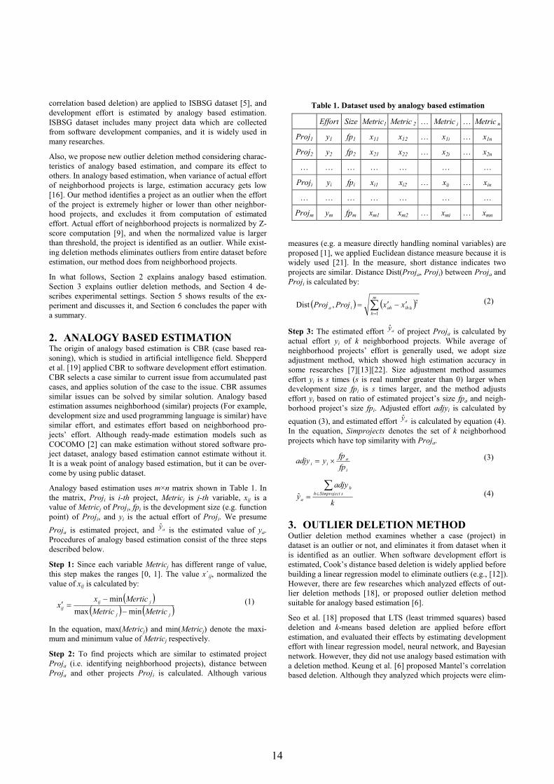
#$ %&��'�(��%'&�A�� $�� B�� /):/?C:/)*:�� '�� /?.:� �� />:/C:/?D:/)?:/)):�� E�� $�� ?� @��&"�F�� G��

��$��#��$�� $�� $��!� ��%�� $�� /)): � �� $�� E�� $��!�� $��!��H��$��

@��$��$��/?+:��I�� $�� $��E�� A��$�� J�� $�� $��(�� I�� #��

A�� $��%�� $��!��!�� K ��#� �� $��!�� !�� !�� />:/?+:� �� J��

�� A�� !�� "��!��

13

��#��H&HL��/M: �� H&HL� �� $��

E�� $�� /?>:��%��$�� $�� $�� E��$��K��N�� /.: � �� K�� $�� $��

�� H�� )� �� H�� D� �� H�� O� �� H�� M� �� H��>��

)$ �&�*' +��%��%'&�A�� &'� �� # ��H��/?.:��&'��&'�� &'�� E�� #��$��I�� K��#�� $��!� �� E�� %�%"%�/):�� $��

E��P��A��?�� $�� K��#� �� $�� Q �� @��

�� #,�H�� /* � ?:��A�� R�� K�� ;�

� ��

��

��

��

��

�� ?#�

�� B�� #� ��#� ��

�� ),� A�� $�� $�� $��# � �� $�� E��

��#��/?: ��(�� /)?:�� $��-��-�� #�� ;�

� � � ��

��

��

?

) -�� )#�

�� -,�A�� Q ��$�� $�� $��!� �� K��$�� /C:/?D:/)):�� H�K� ��$�� *#� �� K� �� $�� $��!�� K� �� $��!�� K� �� E�$�� B��D# �� Q ��B��O#�� B�� $��

�

��

�� D#�

�

��

�

��Q � � � � �O#�

-$ '(�*%��*��%'&��.'��%�� $��#� �� !�� /?):#��J�� K�� /?+: � �� />:��

H�� /?+:�� GAH� �� B��#� �� &�� J�� =��/>:��"��!��E��K��$��

��#$��"��"��

� �� S� �� S��

�� S� �� S� ��

�� S� � �� S� � ��

S� S� S� S� S� � S� � S�

�� S� �� S� ��

S� S� S� S� S� � S� � S�

�� S� �� S� ��

14

�� %��

-$# ��/0�� !�� !�� G�� !�� E� �� !�� O� T�� #�� E�� !��

-$) ��0�� "��!�� !� �� !��A�� E��U� �� />:� �� E��U��?#�� )#� �� $�� D#� �� O#� �� $��#�� M#��D#��

�� @��!�� "��!�� #��"��!��#�� $�� K�� #� ��A�� "��!�� (�� (��

"��!��

?� I��$�� "��!�� $��

)� E�� # ��#��

D� G��!�� $�� B��;�

��!� �� M#�

O� !�� #��O ��$��

-$- &��1�� 1��0�� %�� !�� $��$��E��) ��K��?# �� $�� )# � ��

��D#��$��) ��/?>:��I�� )��E�� !� ��#� �� $�� !��#��%��$��$�� $��A�� $��$��!��J�� $��!�� $��!��H��N�� /.:� �� K� �� !�� $�� V�� $��!�� K��$�� K��$��?� E�� #��#��

��)� H��K�� "�� B��

��N��#;�

��

��

�� >#�

D� E� ��$�� "�� #��V��$�� $�� (��

�Q �� B��;�

��

�� !�� Q � � � �C#�

��B�� !�� $�� $�� ?�>M��M,��#��

H��K� T��#� ��$�� K� ��$�� /C:/?D:��%��K��$��K��$�� $��$�� I��B��D# � ��$��!�� K� �� T� ��$�� K��#�� $�� A�� %�� $�� %��

15

2$ �34��%��&��2$# ��A�� H&HL� �� /M: ��H��&�� H��L�� H&HL#�� $�� )*� �� $�� ?.+.��)**O��

��$��H� �� ..�� A��/??:��$�� #�� -��

�H&HL� �� B�� $�� -�� B��#��H��$�� /??:� �-��B�� E��& �� IW@L�� #��E�� $�� E�� M.D��$��

2$) �5�� A�� #�� E�� (�# � �� "�� '��(�#�/O: ��"��(��'��#�/+: ��&��'��(�#�/?O:��

�� Q �� B��;�

��#� Q�� +#�

��

��Q�

� � � � � � �.#�

��

��QQ�

� � � � � � �?*#�

�

�

�

�

�

��

��

�*Q

QQ

*Q QQ

��

��

�� ??#�

G�� J�� /D:/?*:��"�� ?� �� I�� ?***� �� *� �� ?#�� H�� ?��H�� /?M:�� @��)M#� /O:�� @��)M#��

2$- �� 4 �� (��;�

?� -��B��%�� I��$��# � �� $��#��

)� %��

D� A��K�� ?��)*��E�� B��B��#� ��/?*:#�� B��

O� (��D��

M� (��

>� H��?� ��M� �� ?*� �� E�� ?*�� #��

(��;�

?� -��B��%��

)� (�� ?��)*�� E�� B�� B��

D� (�� )��

O� (��

M� H��?��O��?*��

6$ ��(*��&��%��(��%'&�(�� A��)� ��A�� D��A��)�� -�� $��T��$�� $��T��K��A�� ?*� �� A�� D� �� V��A��D�� A��#��H��M, ��K��

�� E�� #� � �� #� � �� #�� (�� )*�+,��M�D,��"��

16

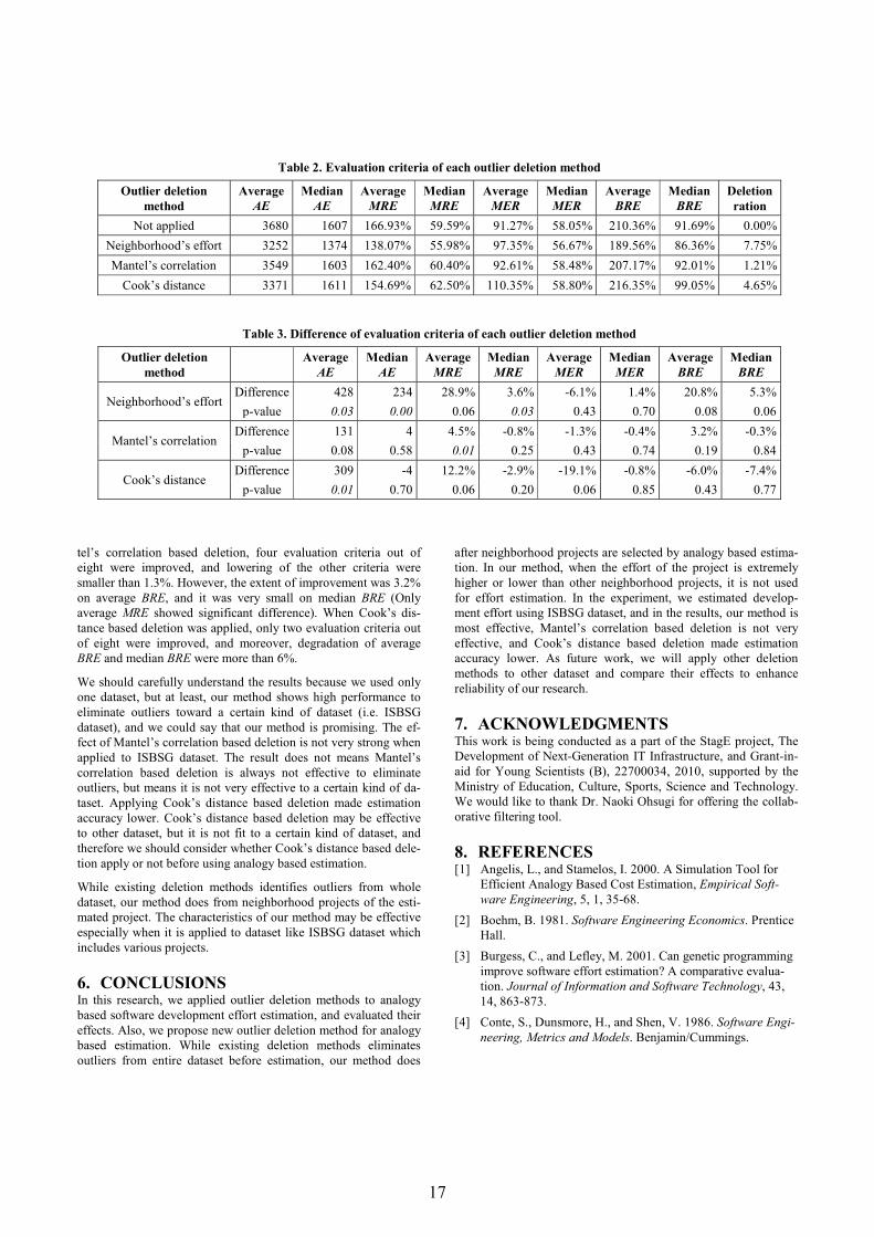
��!�� ?�D,��J�� D�),�� %�� #�� !�� >,��

�� H&HL��# ��A��"��!�� H&HL� �� A�� "��!�� E�� !�� !�� !��

�� $��$��A�� H&HL��$��

7$ �'&�*(�%'&�� E��

��$�� $�� $�� H&HL�� "��!�� !�� E��

8$ ��!&'9*�� &��A�� H��(��$�� A��-��V��L��A�� L�� X��H�� &# � ))C***DO �)*?* � �� "��(�� H�� H��A�� -��V�� %��

:$ ��;��&��/?: E�� G� ��H�� )***��E�H��A��

(��E��&��(�� !��$ �� M �? �DM�>+��

/): &�� &��?.+?��$ ��@��J��

/D: &�� G�� "��)**?��Y�E��%�&�� !��'�� $ �(��!�� OD �?O �+>D�+CD��

/O: �� H� �-�� J� ��H�� Z��?.+>��$ ��)�� !��&�$��T��

��)$��5�� 1�� 1��

'�� 1��

�5 ��

��

�5 ��

��

�5 ��

��

�5 ��

��

��

V�� D>+*�� ?>*C�� ?>>�.D,� M.�M.,� .?�)C,� M+�*M,� )?*�D>,� .?�>.,� *�**,�V��!�� D)M)�� ?DCO�� ?D+�*C,� MM�.+,� .C�DM,� M>�>C,� ?+.�M>,� +>�D>,� C�CM,�"��!�� DMO.�� ?>*D�� ?>)�O*,� >*�O*,� .)�>?,� M+�O+,� )*C�?C,� .)�*?,� ?�)?,�� !�� DDC?�� ?>??�� ?MO�>.,� >)�M*,� ??*�DM,� M+�+*,� )?>�DM,� ..�*M,� O�>M,�

��

��-$�� 5�� 1�� 1��

'�� 1��

� �5 ��

��

�5 ��

��

�5 ��

��

�5 ��

��

V��!��-�� O)+�� )DO�� )+�.,� D�>,� �>�?,� ?�O,� )*�+,� M�D,�� *+*, *+** *�*>�� *+*, *�OD�� *�C*�� *�*+�� *�*>��

"��!��-�� ?D?�� O�� O�M,� �*�+,� �?�D,� �*�O,� D�),� �*�D,�� *�*+�� *�M+�� *+*� *�)M�� *�OD�� *�CO�� *�?.�� *�+O��

�� !��-�� D*.�� O�� ?)�),� �)�.,� �?.�?,� �*�+,� �>�*,� �C�O,�� *+*� *�C*�� *�*>�� *�)*�� *�*>�� *�+M�� *�OD�� *�CC��

�

17

/M: ��H��&�� H��L��H&HL#��)**O��H&HL�(��;�&�� H&HL��

/>: =�� F� �=�� &� ��F�� '��)**+��E��U;�@��H��E��&��H��(��'��(� ��+��$ ��DO �O �OC?�O+O��

/C: =�� "�� (� �@��$ �'� ��H�� "��)**D��E��(��E��G��E��A��B��&��@��+��'�� !�� A�� V�� F��)**D �)D?�)OM��

/+: =�� &� �"��-�� H� �@�� G� ��H�� "��)**?��E��H��'��"��+��'��$ � �?O+ �D �+?�+M��

/.: G�� '� ��"�� "��)***��#�'��&�� !�� '��#��!�� @��J��

/?*:G� �� )**M��H��X��%��K��&��(��"��Y ��+��'�� !��$ ��&�-��(�'��. �� H��)**M �DO��

/??:G� �� "�� (��)**>��H&HL�-��;�� +��'�� !��&�� !��$ ��-'��. �'��F�� &�K�� H��)**> �CM�+O��

/?):"�� (� �"�� H� �I�� I� ��L�� )**+��A� �� ;�E��(�%�&�� !�� $ � �+? �M �>CD�>.*��

/?D:"�� (� �"�� V� �� H��)**D��E�'��E��W��E��'��(��+��'�� !��&�� !��$ ��-'��. �'�� H��)**D �?**�?*.��

/?O:"��K� � �X� �A� �� "� �%K� � �=� ��V�K� � �J��?..O��'��'��-��H��(��"��%�&�� !�� $ � �)C �? �D�?>��

/?M:"[�� \�� =� ��F[�� "��)**M��E��H��@�$��%��I��HB��-��"�� '��(� ��+��$ ��D? �. �CMO�C>>��

/?>:%�� V� �"�� E� �=� �� V� �&� �"� �A�� "� �=� �� A� ��"�� =��)**C��A��(��'��Y��'��J��E��(��'��+��'�� !��&�� !��$ �� &��-��. �"�� H�� H��)**C �D+O�D.)��

/?C:H�� '� ��@�� E��?.++ �G��;��'��(� ��+��$ ��?O �?) �COD�CMC��

/?+:�H� �X� �X�� =� ��&� �-��)**+��E��(��E��H��(��(��%��(��+�� !$��!��$ ��-��/�'��. �G��K�� L�� "��)**+ �)M�D)��

/?.:H�� "� ��H�� ?..C��(��$��'��(� ��+��$ ��)D �?) �CD>�COD��

/)*:H�� =� ��I�� -��?..M��"��G��E��(��H��-��(��'��(� ��+��$ ��)? �) �?)>�?DC��

/)?:A�� E� �A�� &� ��&� �E��)**.��I��$��#��!�� D> �C �?*D)M�?*DDD��

/)):�� I� ��'��F��?...��E��(��H��E��H��(��(�� !��$ �� O �) �?DM�?M+�

18

A Survey of Public Datasets for Comparative EffortPrediction Studies

Sousuke AmasakiOkayama Prefectural University

111 Kuboki, SojaOkayama, Japan

[email protected]

Tomoyuki YokogawaOkayama Prefectural University

111 Kuboki, SojaOkayama, Japan

[email protected]

ABSTRACTBackground: In the past survey, available public datasets for ef-fort prediction study were listed up. In addition, using sufficientnumber of datasets and statistical tests was recommended for validcomparative effort prediction study. Aim: This paper aims to iden-tify a set of useful public datasets in terms of comparative effortprediction study. Method: We sieved 38 public datasets listed inthe past study and PROMISE repository with respect to their avail-ability, variety of features, and applicability of statistical practice.Results: Only 12 public datasets were found to be available anduseful for simple models. For complex models 8 of 12 datasetswere specified. Among 8 datasets, only 3 datasets could keep orig-inal sample size and feature scale. This is because newly proposedeffort prediction methods usually try to improve performance byusing a multiple predictors and many datasets included categoricalfeatures with a level which was not found frequently. To obtainmore datasets, it was needed to adapt remained 5 datasets by casereduction, feature reduction, or numeric conversion. Conclusions:It is difficult to compare multiple effort prediction methods with alarge number of public datasets along with good statistical practice.However, selected datasets must be used for valid study at least.

Categories and Subject DescriptorsD.29 [Software Engineering]: Cost Estimation

General TermsEconomics

1. INTRODUCTIONSoftware cost estimation is still popular and important researcharea. To evaluate performance of a proposed software estimationmodel construction method, datasets from real projects are used inan experiment.

Although it is usually difficult to obtain a dataset from real projects,we can find public datasets in the past study. There are many publicdatasets available to researchers for model evaluation. PROMISErepository[3] now serves 18 downloadable datasets. In [14], the

authors identified 31 datasets freely available to researchers frompublications.

One of criticisms for cost estimation papers is the small number ofdatasets used for evaluation. In [11], it is thus recommended to usemore public datasets shown in [14] and [3]. However, examinationof that listing is needed because comparative effort prediction studywas not considered in [14] and [3]. For example, existence of size-related metric such as lines of code(LOC), Function Points(FP),and effort record was not checked while those are essential infor-mation for models.

In this paper, we thus examined datasets listed in PROMISE repos-itory[3] and [14] in order to specify common datasets available anduseful for comparative effort prediction study. As a result of exami-nation, 12 datasets were found to be available and useful for simplemodels. For complex models 8 of 12 datasets were specified. Forvalid study, these datasets must be used at least.

2. COMPARATIVE STUDY DESIGNIn comparative study, the followings must be considered.

• Simple and Complex models

• Benchmark

• Evaluation procedure

Most of newly proposed software estimation model constructionmethods utilized predictors in order to improve predictive perfor-mance. For example, feature weighting method[1] for Estimationby Analogy(EbA)[18] was proposed to improve EbA by weighingeffects of predictors differently. We called models with multiplefeatures complex models in this paper. On the other hand, simplemodels including only effort and size-related metric are also pop-ular because it is easy to evaluate new methods and to use in caseof small sample size. Both types of models are important but theirrequirements for dataset are different. We thus selected datasets forsimple and complex models differently.

Benchmark is important for comparative study to evaluate howwell performance of a newly proposed model is. For this purpose,conventional models such as linear regression and EbA are oftenused. In fact, most comparative study used one of these methodsas benchmark. Kitchenham recommended to confirm whether anew proposed model outperformed linear regression at least[11].Both models can be used for simple and complex models. In this

19

study, we thus supported that linear regression and EbA are used asbenchmarks.

In comparative study, two types of cross-validation[7] were of-ten used as evaluation procedure: leave-one-out and K-fold cross-validation (CV). Leave-one-out CV can be used for smaller datasetsand it is preferable to K-fold CV in terms of variety of datasets. Itwas also recommended in [11] because of its deterministic prop-erty.

On the other hand, K-fold CV is preferable to leave-one-out CVin terms of evaluation reliability because an estimate obtained us-ing leave-one-out CV has high variance, leading unreliable esti-mates[5]. Furthermore, some performance measures for effort es-timation study cannot be differentiated when leave-one-out CV isadopted. In each round of leave-one-out CV, one test case is usedfor calculating performance measures. That is, MMRE and MdMRE[17] of each test set always have identical value. In case of K-foldCV, MMRE and MdMRE have different values if each test set hasmore than 2 cases.

In [11], bootstrapping[6] was also recommended for performancecomparison based on statistical tests. On the other hand, Kohavirecommended 10-fold CV after comparing to bootstrap[13]. Fur-thermore, property of resampling with replacement used in boot-strapping seems unsuitable for EbA. When a replicated project isplaced in both training and test sets, identical project is always se-lected as the nearest neighbor in EbA. If the number of neighborsis set to 1 for EbA, EbA can estimate exact effort for replicatedprojects.

In this study, we considered 10 × 10-fold CV followed with t-testas evaluation procedure in order to avoid inflated Type I error[4].

3. DATASETSIn this study, we examined published datasets served on PROMISErepository[3] at November 2010 or listed in [14]. PROMISE repos-itory serves datasets as readable text file which can include com-ments. From this repository, we selected datasets which contain acomment regarding information of projects or a citation they wereused. Datasets from [14] were collected from three journals: Trans-actions on Software Engineering, Information & Software Tech-nology, and Journal of Systems & Software. After removing du-plicates, we prepared an initial set of 38 datasets shown in Table1.

We then checked these datasets in terms of availability. First andsecond columns of Table 1 show whether a dataset can be obtainedactually from referenced papers in [14] or PROMISE repository. Ifboth columns of a dataset were marked as ‘N’, this dataset is noteasily available.

We found that 7 datasets were not easily obtained from referencedpapers and PROMISE repository. ID 3, 4, and 30 were not shownin an original paper[2] cited in [14] and this paper said that an oldbook published in 1986 contains these datasets. We assessed ID12 as unavailable though it was registered in PROMISE reposi-tory. This is because the number of features in this dataset was veryfewer than that described in a referenced paper[18]. The number offeatures was 29 according to [18] while dataset held on PROMISErepository included only 6 features (excluding logarithm of effortand size.) Referenced papers of the others did not have a dataset,a pointer to a paper, nor a book which may include corresponding

datasets.

In the following sections, remained 31 datasets were examined.

4. SELECTION FOR SIMPLE MODELSSimple models usually estimate effort from single size-related met-ric such as KSLOC(kilo source LOC) and FP. Thus, size-relatedmetric must be included in a dataset. Sample size is also importantfor evaluation procedure and reliability of results.

Datasets were selected by evaluation criteria related to these points.

4.1 Effort and Size RecordsThird and fourth columns of Table 1 show whether a dataset in-cludes effort and size records. Here, unavailable 7 datasets in theprevious section were ignored and blanks were placed.

We found that 6 datasets did not include effort or size metric. ID25, 26, and 27 did not include effort records. These datasets onlyincluded KSLOC and size related-metrics such as the number ofscreens and were used to construct sizing models[15]. ID 5 in-cluded 3 features: actual effort, expert estimates, and company la-bels. ID 18 and 19 only included actual effort and experts estimates.These datasets were not suitable for comparative effort estimationstudy because an expert estimate was rarely used as the only pre-dictor in a software estimation model.

4.2 Sample SizeIn many situations, a fitted regression model is likely to be reliablewhen the number of predictors p (the number of candidate predic-tors if using variable selection) is less than m/10 or m/20, wherem is total sample size[7]. Following this rule, at least, a dataset hasto include more than 10 projects in case of simple models. Further-more, the size of training subsets becomes smaller when the sizeof training set in evaluation procedure is considered. In case of 10-fold CV, sample size N must be N > 12 because 9/10 · N > 10must be held.

To make performance measures such as MMRE and PRED(25)[17]reliable, the size of test set must be larger as described in Section 2.If the size of test set must be always equal or larger than 3, thoughperformance measure based on 3 results is still less precise and lessfine-grained, sample size must be equal or larger than 30 because1/10 ·N ≥ 3 must be held.

Fifth column of Table 1 shows whether a dataset has the sufficientnumber of projects. Here, we marked as ‘Y’ if a dataset had 30or more projects; otherwise we marked as ‘N’ with its size. Thiscolumn indicated that 13 datasets were too small to be used in com-parative effort prediction study.

Finally, 12 public datasets were remained for comparative effortprediction study of simple models.

5. SELECTION FOR COMPLEX MODELSComplex models assume multiple predictors. For instance, CARTselects and combines predictors so that a software effort estimationmodel achieves higher prediction accuracy. Sample size is moreimportant for reliable evaluation of complex models. Furthermore,types of candidate predictors are also important. If there is discretevariables, using k-fold CV may be difficult.

20

Table 1: Public datasets from [14] and [3]ID Name Paper PROMISE Effort Size Sample Size Multiple Features Categorical

1 Abran-Robillard Y N Y Y N(21)2 Albrecht-Gaffney Y Y Y Y N(24)3 Bailey-Basili N N4 Belady-Lehmann N N5 Shepperd-Cartwright Y N Y N6 BT-software-houses Y N Y Y N(10)7 BT-systemX Y N Y Y N(10)8 COCOMO N Y Y Y Y Y(16) Y(16)9 CSC Y N Y Y Y Y(2) Y(2)

10 Desharnais N Y Y Y Y Y(7) Y(1)11 Dolado Y N Y Y N(24)12 Finnish N N13 Hastings-Sajeev Y N Y Y N(8)14 Heiat-Heiat Y N Y Y Y Y(1) N15 ICL Y N Y Y N(10)16 Jørgensen97-A Y N Y Y N(16)17 Jørgensen97-B Y N Y Y N(20)18 Jørgensen04-X Y N Y N19 Jørgensen04-Y Y N Y N20 Kemerer Y Y Y Y N(15)21 MERMAID1 N N22 MERMAID2 Y N Y Y Y Y(1) Y(1)23 Misic-Tesic Y N Y Y N(7)24 Miyazaki et al.1 Y Y Y Y Y Y(7) Y(1)25 Miyazaki et al.2 Y N N Y26 Miyazaki et al.3 Y N N Y27 Miyazaki et al.5 Y N N Y28 Moser-etal Y N Y Y Y Y(1) Y(1)29 Telecom Y Y Y Y N(18)30 Wingfield N N31 WSD1 N N32 WSD2 N N33 cocomonasa_v1 Y Y Y Y Y(15) Y(15)34 cocomo_sdr Y Y Y N(12)35 Maxwell Y Y Y Y Y(22) Y(22)36 NASA93 Y Y Y Y Y(20) Y(20)37 usp05 Y Y Y Y Y(14) Y(14)38 usp05ft Y Y Y Y Y(12) Y(12)

We evaluated 12 datasets selected in the previous section by criteriarelated to these points.

5.1 Multiple FeaturesComplex models utilize multiple features. Therefore datasets mustinclude multiple features for comparative effort prediction study.

Seventh column of Table 1 shows whether a dataset includes atleast one feature other than KSLOC and FP-variants. The num-ber following ’Y’ indicates the number of features. For example,Desharnais (ID 10) has 7 features because unadjusted and adjustedFP were ignored and elements such as Transactions were counted.Inappropriate features such as duration were also ignored.

As a result, all 12 datasets were remained.

5.2 Sample SizeUsually the size of datasets for complex models must be larger thanthat for simple models. For instance, if linear regression models

using size-metric and one feature as predictors are considered asbenchmark, a dataset must include more than 23 projects accordingto the rule described in subsection 4.2.

Here, we left all 12 public datasets because they all have equalor more than 30 projects and complex models based on linear re-gression with two predictors can be constructed at least. Althoughadditional samples might be needed for other models, we did notconsider that case here.

5.3 Categorical FeaturesTen-fold CV can be applied to a dataset with categorical features ifeach training subset includes all levels of each categorical featureincluded in corresponding testing subset. To satisfy this condition,each level of a categorical feature must be found in more than N/10records. If there is categorical feature with a level which was foundless than N/10 times, case reduction, feature reduction, or numericconversion is needed.

21

Eighth column in Table 1 shows whether a dataset includes categor-ical feature(s) and the number of them. Datasets having categoricalfeatures can be classified into two groups:

• a few categorical variable(s) are included(5 datasets) and

• many categorical variables are included(6 datasets).

In the first group, Desharnais(ID 10) and MERMAID2(ID 22) haveone categorical feature which satisfies the condition for levels. Acategorical feature of Desharnais dataset has three levels each ofwhich was found in more than one-eighths of records. A categoricalfeature of MERMAID2 dataset also has two levels each of whichwas found in at least one-thirds of records. Thus, they can be usedfor comparative study as is.

CSC(ID 9), Miyazaki1(ID 24), and Moser-etal(ID 28) datasets haveone or two categorical features with a level which was found lessthan N/10 times. These categorical features were not used as pre-dictor in original papers[12, 15, 16].

Miyazaki1 has one categorical feature representing companies. Forthis dataset, case reduction is useless because there is no level withmore than N/10 records. Concatenation of levels or numeric con-version cannot be applied because this feature is nominal scale andthere is no knowledge of relations among companies. Thus, weconcluded that feature reduction is the best way for comparativestudy. We think that this feature has too many levels for samplesize and is useless for estimation.

Moser-etal has one categorical feature representing project charac-teristics. If case reduction is applied, the size of this dataset be-comes lower than 30. Concatenation of levels or numeric conver-sion cannot be applied because it is nominal scale. Feature reduc-tion makes this dataset inappropriate for complex models becauseit has only one feature.

CSC has two categorical features representing clients and projecttypes. Case reduction decreased the size of this dataset to 106. Italso reduced the numbers of client types and project types to 1 and2, respectively. Thus, one categorical feature of project types wasremained. In [12], the authors considered simple models and usedseveral types of partitioning based on categorical features. On theother hand, we considered complex models and thus case reductionwas prefer to feature reduction.

In the second group, all datasets have multiple categorical featureswith a level which was found less than N/10 times. It is difficultto adapt these datasets to comparative study by case reduction. Be-cause there are many categorical features and case reduction basedon a categorical feature may influence on the other features. Fur-thermore, large portion of cases may be reduced for satisfying equalto or more than N/10 cases for all levels. Concatenation and fea-ture reduction are also difficult because there is no general way forall possible effort estimation models. Thus, numeric conversionwas first considered for this group.

Most of categorical features in COCOMO(ID 8), cocomonasa_v1(ID 33), and NASA93(ID 36) were COCOMO or COCOMO II at-tributes. For these attributes, adjustment factors were often used inthe past study. With adjustment factors, 10-fold CV can be appliedto COCOMO and cocomonasa_v1.

NASA93(ID 36) dataset included some nominal scale features hav-ing a level which was found less than N/10 times. For develop-ment mode among these features, case reduction is helpful becausethis feature can satisfy N/10 rule by removing one level with 3projects. Other nominal features were looked as less important forsoftware estimation models. In fact, they were not used in the paststudy. Thus, we concluded that NASA93 dataset can be used afternumeric conversion, small case reduction, and feature reduction areapplied.

Maxwell(ID 35) dataset contains ordinal features and nominal fea-tures. Numeric conversion can be applied to ordinal features. Fourout of 7 nominal features have a level which was found less thanN/10 times. All of them were looked important and feature reduc-tion was not preferable to case reduction. Case reduction based onthese features reduced the size of this dataset from 62 to 46. Threenominal features were also removed because they have only onelevel in this reduced dataset.

Many features in usp05 and usp05ft datasets(ID 37 and 38) werecategorical with many levels and it is difficult to determine the wayfor adapting it to comparative study. Thus, we concluded that 10-fold CV cannot be applied for these datasets.

As a result, 9 datasets were remained.

5.4 Detailed ExaminationDesharnais, Heiat-Heiat, MERMAID2, and Miyazaki1 are prefer-able to the other datasets. Because they could keep original samplesize and feature scale. Here, we examined 4 datasets selected interms of usefulness and reliability. Since Desharnais has alreadybeen examined in [11], we examined other 3 datasets.

5.4.1 Heiat-Heiat dataset[8]This dataset came from projects completed for private and publicorganizations in Billings, Montana. There was no missing value.These projects were selected on the basis of 6 attributes so that thedataset consists of homogeneous projects.

Figure 1 shows a scatterplot of FP and Effort for all 35 projects.There are no apparent skewness, no heteroscedacity, and no outlier.

●

●

●

●

●

●

●

●

●

●

●

●

●

●

●

●

●

●

●

●

●

●

●

●

●

●

●

●

●

●●

●

● ●

●

50 100 150 200 250 300

150

200

250

300

350

FP

Effo

rt

Figure 1: Heiat-Heiat dataset

This dataset included a feature representing the sum of total num-ber of corrected relationships at data stores and total number of

22

data flows which connect the system to external entities. Heiat etal. proposed this metric, called REIO, as alternative measure ofsize such as LOC[8]. In fact, REIO and LOC were highly corre-lated (Spearman’s ρ is 0.93.) These facts imply that the differencebetween simple and complex models will be subtle.

Thus, we concluded that this dataset was inappropriate for compar-ative effort prediction study in terms of variety of features.

5.4.2 Miyazaki1 dataset[15]This dataset came from 48 projects in 20 companies. There is nomissing value. All systems were newly developed except for oneproject, in which more than half of its code was adapted from anexisting system[15].

●●

●● ●●

●●●

●●●

●

●

●●

●● ● ●●●

●● ●●

●

●

●

●

●

●

●● ●●●

● ●● ●●

●

●● ● ●●

0 100 200 300 400

050

010

0015

00

KLOC

Effo

rt

Figure 2: Miyazaki1 dataset

Figure 2 shows a scatterplot of KLOC and Effort. There is oneoutlier. There is skewness and small heteroscedacity. It looks as ifall projects except for the outlier have similar relationships betweensize and effort.

Six continuous features in this dataset can be classified into threepairs with respect to their semantic similarity. Features of each pairwere also highly correlated. Even if a half of features were droppedby a software estimation model construction method, the others stillremain.

In this study, we concluded that the dataset may be useful for com-parative effort prediction study because there is room for modelselection and optimization.

5.4.3 MERMAID2 dataset[10]This dataset has one categorical feature representing new projectsand enhancement projects. Here, dividing the dataset into twoproject types is not appropriate approach because the number ofnew projects is less than 10.

There is two missing values on a categorical value. If raw FP isused instead of adjusted FP, other 2 projects must also be removedbecause of missing values. Figure 3 shows a scatterplot of adjustedFP and Effort of 28 projects. The dataset has two outliers[10].There is skewness and heteroscedacity.

EEEEEEE N NE NEE

NE

N

N

E N

E

E

NEE E

EEE

0 500 1000 1500

010

000

3000

050

000

AdjFP

Effo

rt

Figure 3: Mermaid2 dataset (N = New projects, E = Enhance-ment Projects)

From these characteristics, we concluded this dataset was some-times inappropriate for comparative effort prediction study. Be-cause this dataset is too small to perform 10-fold CV when missingvalues must be removed. We determined to leave this dataset.

Table 2 shows remained 8 datasets. Size and the number of fea-tures are from reduced datasets. Marks ‘FR’, ‘CR’, and ‘NC’ in-dicate feature reduction, case reduction, and numeric conversion,respectively.

As a result of examination, available 38 public datasets were de-creased to 12 datasets for simple models and to 8 datasets for com-plex models.

6. DISCUSSIONIn subsection 5.3, several types of preprocessing was applied todatasets in order to adapt them to comparative effort predictionstudy. These preprocessing have drawbacks.

The problems of case reduction are decreasing of size and changeof population. In this study all selected datasets have sufficientnumber of projects and the size was not problem. Case reductionin this study was based on categorical feature having a level whichwas found less than N/10 times. Thus, population was changed butit becomes more homogeneous. Homogeneity of dataset is consid-ered as important property for effort estimation.

Most of reduced features in this study were due to case reduction.Thus, dropped features seemed less important at least for reducedhomogeneous datasets.

Although using adjustment factors is like a calibration, not con-struction of software estimation model, it was popular method fordealing COCOMO drivers. Numeric conversion of ordinal scaleswas also popular though this conversion implicitly assumes linearrelationship among levels. To manage these problems, feature sub-set selection may be useful. When all selected categorical featuressatisfy N/10 rule, these features can be used as is.

This study did not use technique concatenating levels though usingit instead of case reduction may also be useful. Because it is dif-ficult to automate concatenation process because human decision

23

Table 2: Selected Datasets for Complex ModelsNo. Name Size Features FR CR NC

8 COCOMO 63 16 X9 CSC 106 1 X X

10 Desharnais 77 722 MERMAID2 30 124 Miyazaki1 48 6 X33 cocomonasa_v1 60 15 X35 Maxwell 46 19 X X X36 NASA93 90 16 X X X

plays an important role as shown in [9].

7. CONCLUSIONIn this paper, we examined the list of public datasets in [14] andPROMISE repository. As a result, we found 12 of 38 datasets wereonly appropriate for comparative effort prediction study of simplemodels. For complex models, this number was decreased to 8.Among 8 datasets, only 3 datasets could keep original sample sizeand feature scale. We thus concluded that using one or two publicdatasets is insufficient but there is not so many datasets suitable forcomparative study.

To make effort prediction study of complex models more compa-rable, we recommend to use those 3 datasets at first. In practicalview, CSC and MERMAID2 has too few features to evaluate com-plex models such as CART though. In this case, it is recommendedto consider remained 5 datasets next to Desharnais. The fact thatmany datasets need to be changed for use implies that repositorieslike PROMISE should provide detailed and recommend prepro-cessing sequence for removing heterogeneity among comparativestudies.

8. REFERENCES[1] M. Auer and S. Biffl. Increasing the accuracy and reliability

of analogy-based cost estimation with extensive projectfeature dimension weighting. In Proc. of the 2004International Symposium on Empirical Software Engineering(ISESE’04), pages 147–155, 2004.

[2] R. D. Banker, H. Chang, and C. F. Kemerer. Evidence oneconomies of scale in software development. Informationand Software Technology, 36:275–282, 1994.

[3] G. Boetticher, T. Menzies, and T. Ostrand. PROMISErepository of empirical software engineering data.http://promisedata.org/repository, WestVirginia University, Department of Computer Science, 2007.

[4] R. R. Bouckaert. Choosing between two learning algorithmsbased on calibrated tests. In Proc. of 20th InternationalConference on Machine Learning, pages 51–58, 2003.

[5] B. Efron. Estimating the error rate of a prediction rule:Improvement of cross-validation. Journal of the AmericanStatistical Association, 78:316–330, 1983.

[6] B. Efron and R. J. Tibshirani. An Introduction to theBootstrap. Chapman & Hall, 1993.

[7] F. E. Harrel. Regression Modeling Strategies. Springer, 2001.[8] A. Heiat and N. Heiat. A model for estimating efforts

required for developing small-scale business applications.Journal of Systems and Software, 39:7–14, 1997.

[9] B. Kitchenham. A procedure for analyzing unbalanced

datasets. IEEE Trans. on Software Engineering,24(4):278–301, 1998.

[10] B. Kitchenham. The question of scale economies in software— why cannot researchers agree? Information and SoftwareTechnology, 44(1):13–24, 2002.

[11] B. Kitchenham and E. Mendes. Why comparative effortprediction studies may be invalid. In Proc. of PROMISEWorkshop 2009, 2009.

[12] B. Kitchenham, S. Pfleeger, B. McColl, and S. Eagan. Anempirical study of maintenance and development estimationaccuracy. Journal of Systems and Software, 64:57–77, 2002.

[13] R. Kohavi. A study of cross-validation and bootstrap foraccuracy estimation and model selection. In Proc. ofInternational Joint Conference on AI, pages 1137–1145,1995.

[14] C. Mair, M. Shepperd, and M. Jørgensen. An analysis of datasets used to train and validate cost. In Proc. of 1stInternational Workshop on Predictor Models in SoftwareEngineering(PROMISE’05), 2005.

[15] Y. Miyazaki and M. Terakado. Robust regression fordeveloping software estimation models. Journal of Systemsand Software, 27(1):3–16, 1994.

[16] S. Moser, B. Henderson-Sellers, and V. B. Mišic. Costestimation based on business models. Journal of Systems andSoftware, 49:33–42, 1999.

[17] D. Port and M. Korte. Comparative studies of the modelevaluation criterions MMRE and PRED in software costestimation research. In Proc. of 2nd InternationalSymposium on Empirical Software Engineering andMeasurement (ESEM’08), 2008.

[18] M. Shepperd and C. Schofield. Estimating software projecteffort using analogies. IEEE Trans. on Software Engineering,23(11):736–743, 1997.

24

Faults and Verification

25

Reconstructing Fine-Grained Versioning Repositories withGit for Method-Level Bug Prediction

Hideaki HataDept.of Information Systems

EngineeringOsaka University

Osaka, [email protected]

Osamu MizunoDept. of Information ScienceKyoto Institute of Technology

Kyoto, [email protected]

Tohru KikunoDept.of Information Systems

EngineeringOsaka University

Osaka, [email protected]

ABSTRACTChange metrics derived from software repositories are known tobe effective for bug prediction. However, bug prediction basedon change metrics is limited to file-level because existing SCMrepositories stores file histories. To tackle fine-grained (method-level) bug prediction, we try to establish fine-grained versioning forrepositories. This paper presents an automatic technique construct-ing software repositories that can manage method histories. We uti-lize Git, one software configuration management (SCM) systems,and reconstruct fine-grained versioning repositories from existingrepositories. We utilize these method-level versioning repositoriesfor method-level bug prediction with one eclipse related project.The result shows that method-level change metrics are effective formethod-level bug prediction.

Categories and Subject DescriptorsD.2.7 [Software Engineering]: Distribution, Maintenance, andEnhancement—Version control; D.2.8 [Software Engineering]: Met-rics; D.2.9 [Software Engineering]: Management—Software con-figuration management

General TermsManagement

Keywordsfine-grained versioning, software repository, bug prediction, method-level, Git, software evolution

1. INTRODUCTIONSoftware configuration management (SCM) repositories have beenwidely targeted for many research areas because of their rich prod-uct and process related data. Bug prediction is one of those researchareas. Many studies reported that change metrics derived from soft-ware repositories are effective for bug prediction [9, 11, 13, 20, 23,25].

SCM systems can track the history of files and record, for ex-ample, existence periods, previous operations, and the reasons ofthe changes. Therefore, change metrics, such as age, number ofchanges, bug fixes are easily available from software repositories.Previous studies conducted file-level bug prediction based on filehistories. In this paper, we tackle method-level bug predictionbased on method histories because we think it is easy to localizebugs if the size of predicted modules is smaller.

From existing software repositories, seeing method histories is notso easy. It is reported that though there are lots of refactorings,which include the file relocations and method signature changes,developers do not always leave in commit logs enough informationdescribing the changes they did in commit logs [21]. Since gen-eral repositories do not control method histories explicitly, we can-not obtain rich information for methods as for files. In this paper,we prepare method-level version control repositories before miningchange metrics.

The concept of fine-grained version control can be seen in Or-well [27] as method-level version control in object-oriented pro-gramming. Though several tools have been proposed to supportfine-grained versioning, no such a tool has been actually integratedwithin widely used SCM systems [6]. Since existing repositoriesremain file-level versioning, what we have to do is converting exist-ing repositories into fine-grained versioning repositories. Thoughthere are some studies tackling extraction of method histories fromrepositories, we try not only to extract method histories but alsoto controlling method histories. For the purpose of converting, weutilize Git, one SCM system.

Herraiz et al. presented software repository evolution from CVS,Subversion to Git, and insisted that those improvements made repos-itories research friendly [16]. Bird et al. studied both promiseand peril of Git [3]. Though Git is known for the decentraliza-tion of source code management, we found that Git architectureis also useful for our purpose. “Directed acyclic graph (DAG),”“origin analysis,” and “revisionist history,” which are Git featuresexplained by Bird et al. [3], are also desirable for our purpose. Inaddition, “snapshots” is also an important feature.

The rest of the paper is structured as follows. Section 2 introducesfour Git features, which is important for our purpose of reconstruc-tion. Then, Section 3 presents a technique of reconstructing reposi-tories from existing repositories based on Git. Section 4 shows use-fulness of our fine-grained versioning repositories with a case studywith an open source project. In addition, we utilize fine-grainedversioning for method-level bug prediction. Section 5 introduces

27

(a) Difference-based storing (Subversion)

(b) Storing snapshots (Git)

Figure 1: Differences in storing version data

Figure 2: A subgraph of the Git DAG of commits leading up to2.1 release 1 of Android

related work. Finally, we concluded this paper in Section 6.

2. GIT FEATURESRecently Git attracted the attention of some researchers [3, 14, 16].Though decentralization is one of the main characteristics com-pared to Subversion, there are some other distinctions. In this sec-tion, we introduce four Git features that are desirable for recon-structing fine-grained versioning repositories.

2.1 SnapshotsOne of the major differences between Git and Subversion (or CVS)is the way it stores version data. Figure 1 shows an example ofversion control of three files. The file A is changed in version 2and version 3, the file B is changed in version 3 and 4, and the fileC is changed in version 2. Subversion stores a set of files and thechanges made to each file over time, as illustrated in Figure 1 (a).Figure 1 (b) shows how Git stores data. Git stores each snapshotof what all files look like at each commit. To be efficient, if fileshave not changed, Git does not store the files but stores links to theprevious files that have been already stored. What is import is thateach file is stored without begin connected to files in the previousversion.

2.2 DAGAs explained in [3], parent-child relation in commits is representedas a graph in Git. A commit have more than or equal to one par-ent except for the initial commit. Since no commit cannot be its

Figure 3: Retaking snapshots without changing commit DAG

own ancestor, the graph is a directed acyclic graph (DAG). Figure2 shows an example of commit DAG. As shown in the example,merging commits have more than one parent commit. As seen inFigure 1 (b), each version of one file is stored in each snapshot sep-arately. Each commit knows its snapshot. The orders or relationsof file versions are kept as DAG of commits relation.

2.3 Origin analysisAs explained by Bird et al., Git tracks the file content history [3].Therefore, files with the same content but different names or loca-tions in the parent and child commits are found as a renamed ormoved file. This origin analysis is not limited to identical contentbut also similar content. When file paths are changed, often filescontent are also modified. Even in such cases, Git is able to de-tect relationships between changes if the file contents are similarenough. Origin analysis is conducted by checking that the amountof deletion of the original content and insertion of new content islarger than the threshold, which is set to 50% of the size of smallerfiles (original or modified). Therefore, if deletion or insertion isless than 50%, two files in parent and child commits are detectedas moving or renaming. The threshold value can be changed. Withthis feature, developer can recognize the renaming and moving.

2.4 Rewriting historiesBird et al. introduced rewritable Git histories from the aspect ofDAG changing [3]. Git allows a repository owner to rearrange DAGretaining each snapshot. This rewriting is commonly conducted tosimplify commit relation. In addition to that rewriting, it is alsopossible to change snapshots by calling filter-branch command1.As shown in Figure 3, each snapshot can be changed retaining itsDAG. One of the uses of this rewriting is getting rid of a subset ofunnecessary files.

3. REPOSITORY RECONSTRUCTIONAs seen in Section 2, there are some features in Git different fromSubversion. We found that these features are desirable for our pur-pose of reconstructing fine-grained versioning repositories. In thisSection, first we show the fundamental idea of our approach, andthen we explain our technique and its implementation.

3.1 IdeaFor fine-grained (method-level) version control, what we have to dois making each method controllable in repositories. Since reposito-ries are able to control file histories, it is possible to control method

1This command is not limited to changing snapshots retainingDAG. It is also possible to change DAG.

28

Figure 4: Retaking a snapshot for method storing

Figure 5: File structure

histories if each method is stored as a file. As explained in Section2.1, Git stores existing files at each commit as a snapshot. In ad-dition, it is possible to retake snapshots without changing commithistory relation as stated in Section 2.4.

Figure 4 shows a concept of our approach. We retake each snap-shot and replace it with a snapshot that includes additional methodfiles. This replacement enables us to control method histories liketraditional file histories. In original snapshot S, there exist originalfiles F ,G, andH . To retake snapshot S′, methods exist in each fileare copied and stored as files. Each snapshot is retaken separatelywithout retaining file-level and method-level relations. Relationsbetween methods will be detected by Git origin analysis. If meth-ods are moved or renamed, the corresponding methods should bedetected automatically, and method histories are managed by Git.

3.2 TechniqueTo retake the snapshots, we have to obtain the list of Java files thatexist in the original snapshots. From each Java file, exiting methodsare extracted and copied to individual files.

For storing method files, file structures are designed as Figure 5.Here, we explain the case of Java language. Each java file is savedas it is (file-name.java in Figure 5); if there are methods in the file,a directory named as the file’s name (file-name) is created; files ofmethods are saved in the directory; these files are named by theirmethod signatures. For simplicity, we limited to methods in top-level classes in this paper. Methods in inner classes or anonymousclasses are ignored. In addition, abstract methods are not stored.Directories and files in gray space of Figure 5 are newly preparedfor new snapshots.

Changes of method signatures correspond to file name changes and

moving of methods correspond to moving files. If a method isdeleted in a commit and reappear in later commit, Git can outputits history including disappearing periods. As described in Section2.3, the origin analysis is conducted based on file content similarity.Based on the threshold of content similarity, corresponding meth-ods are identified. If two methods are highly similar, it is rationalto detect them as corresponding methods. However, they mightbe corresponding methods in spite of not high similarity. In Sec-tion 4.1, we manually investigate whether found method origins arecorrect or not.

3.3 ImplementationThough existing repositories are not in Git system, it is possibleto convert them to Git repositories for most SCM systems, as ex-plained as ninth promise of Git in [3]. Therefore we can concen-trate on reconstruction of Git repositories. In this paper, we targetrepositories of software written in Java language. As stated in Sec-tion 2.4, filter-branch command can be used for our purpose with a–tree-filter option. With this option, each snapshot appears in work-ing directory and we can retake a snapshot after conducting someprocedure. For our purpose, we copy the methods before retakingthe snapshots. For locating the methods in Java files, we used thesource code analysis tool MASU2, which is an open source tool. Itutilizes ANTLR for parsing source code [1].

4. ANALYSISIn this Section, we investigate the usefulness of fine-grained ver-sioning repositories. First, we examine whether Git origin analy-sis is useful for method-level origin analysis. Next, we conductedmethod-level bug prediction based onmethod-level changemetrics.We targeted the WTP incubator project in Eclipse3 for the analysis.This project is written in Java and is maintained with Git4. Wecloned the Git repository on the 15th November, 2010.

4.1 Origin analysis evaluationGit detects origins of methods after changing names or location ofthe methods. When contents of methods are modified, detectionof corresponding methods is conducted by calculating similarityof potential method pairs. If similarity is greater than or equal tothreshold, the potential method pairs are detected as renamed meth-ods as stated in Section 2.3. Users can change the threshold.

In this Section, we classify the method pairs according to similarityvalues to see the impact of the threshold and investigate whetherdetected method pairs seem to be correct or not. To knowwhether itis correct matching or not, we investigate every matching methodsbased on their method signatures and method paths. Since it isdifficult to distinguish correct matches from mismatches perfectly,we count the number of obvious mismatches.

As shown in Figure 6, the found method matches are classifiedbased on similarity values from 0% to 100% at 10% intervals. Tosee the impact of the text size for the similarity calculation, theresult is summarized separately, (a) different lines (deletion lines+ insertion lines) is less than 10, and (b) the others. Dark graybars represent the numbers of detected obvious mismatches, andthe numbers of other matches are represented as light gray bars.

2http://sourceforge.net/projects/masu/3http://www.eclipse.org/webtools/incubator/4http://git.eclipse.org/c/webtools/org.eclipse.webtools.incubator.git/

29

(a) different lines < 10

(b) different lines >= 10

Figure 6: Method matches based on a threshold

After checking manually, we found that automatic method match-ing based on Git works relatively well. There is a large number ofmethod pairs whose similarity value is 100%, which means thesemethods have been renamed without being modified. There are fewobvious mismatches if the similarity is greater than 20% whetherthe number of different lines is less than 10 or not.

Though the results of origin analysis evaluation may depend onprojects or applications, line-based matching works relatively wellas shown by Kim [19]. We think this is because there should befew cases where a newly created method is similar in content toa deleted method when the created and the deleted methods areindependent of each other. We think that developers tend to commitsimple changes, that is, the number of matching candidates is smallandmatching pairs are easy to find, not to confuse module histories.

4.2 Bug Prediction Based on Method HistoryTable 1 shows metrics we collected in this paper. The threshold oforigin analysis is the default value (50%). This means that methodsare regarded as newly created if most lines (>50%) are changedwhen names or locations of the methods are changed. In this paper,file-level bug prediction is also conducted to evaluate method-levelbug prediction. For file-level bug prediction, the same metrics inTable 1 are collected except for NCHG_SIG.

Whether modules are faulty or not is decided by using the SZZalgorithm [26]. We obtained bug reports from the bug databases(Bugzilla) under the following conditions. The type of these faultsis “bugs”; therefore, these faults do not include any enhancementsor functional patches. The status of faults is either “resolved”, “ver-ified”, or “closed”, and the resolution of faults is “fixed”. This

Table 1: Change metrics collected in this paperMetrics DescriptionNCHG Number of individual changesNFIX Number of bug fixesNAUTH Number of authorsAGE Existing periodITVAL_{MAX, MIN} Period of {maximum, minimum}

interval between commitsLOC_{ADD, DEL} Some of {added, deleted} lines of

code between first and last revisionsNCHG_BUG_INTRO Number of changes that is in

commits that include bug-introducingchanges to other methods

NCHG_BUG_COPL Number of changes that is incommits that include changes to othermethods (change coupling)

NCHG_SIG Number of method signature changesNCHG_FILE Number of file name changesNCHG_PCK Number of package changesIS_FAULTY Faulty or not. Dependent variable in

prediction models

Table 2: Results of the 10-fold cross validation(a) Method-level

Model Recall Precision F1

Naive Bayes 0.704 0.030 0.057Logistic regression 0.556 0.750 0.638J48 0.593 1 0.744

(b) File-levelModel Recall Precision F1

Naive Bayes 0.778 0.073 0.134Logistic regression 0.111 0.286 0.160J48 0.389 0.875 0.538

means that the collected faults have already been fixed and havebeen resolved, and thus fixed revisions should be included in theentire repository. The severity of the faults is either “BLOCKER”,“CRITICAL”, or “MAJOR” in order to remove trivial bugs. Her-raiz categorized these severity categories as important and the oth-ers without ENHANCEMENT as non-important [15].

We conducted a 10-fold cross validation on a snapshot with the tag,v20090510. There are 4, 733 methods including 27 faulty meth-ods, and there exist 698 files including 18 faulty files in this snap-shot. We adopted the WEKA data mining toolkit [29] for buildingbug prediction models. We built the following three models: naiveBayes, logistic regression, and J48. For the evaluation of the exper-iment, we use three measures: Recall( TP

TP+FN), Precision( TP

TP+FP), and F1( 2×recall×precision

recall+precision)5.

Table 2 shows the method-level and file-level results. The precisionvalues of naive Bayes are low because of lots of false positive. Asa result, F1 values of naive Bayes are low. Though the ratio offaulty modules per entire modules in method-level is lower thanfile-level, F1 values in method-level are superior to file-level fromlogistic regression and J48 models. Those two models achievedmore than 0.63 F1 values. Though bug prediction is conducted ononly one project, it seems that method-level change metrics may beeffective for method-level bug prediction.

5. RELATEDWORK5TP (true positive), TN (true negative), FP (false positive), FN(false negative)

30

Table 3: Comparison of method history analysisMethod/Tool/Authors Objective Relationship analysis target StoringJDiff [2] detection of structural changes name -C-REX [12] assessment of change propagation tools calls, tokens XMLOrigin analysis [8] detection of merging & splitting name, code metrics, calls BEAGLE repository

(relational database)S. Kim et al. [19] detection of renaming name, code metrics, calls, text -UMLDiff [31] detection of structural changes name, structure -RefactoringCrawler [7] detection of refactorings tokens, structure XMLWeißgerber and Diel [28] detection of refactorings name, structure, text -SemDiff [5] recommending adaptive changes name, calls, structure -LSdiff [17] detection & representation of systematic changes name, calls, structure -AURA [30] detection of structural changes calls, text -This paper fine-grained versioning text Git

Bug prediction based on change metrics. Graves et al.have studied software change history and found that if moduleswere changed many times, the modules tended to contain faults [9].In addition, they found that if modules had not changed for oneyear, the rate of the modules containing faults would be low. Na-gappan and Ball examined code churn, which is a measure of theamount of code change, and showed that relative code churn ishighly predictive of defect density [22]. Ostrand et al. showedthat fault and modification history of the file from previous releasecould be predictive of faults in the next release of a system [23].Schröter et al. have studied the correlation with past failure com-ponent history and failure-prone components [25]. They analyzedSCM repositories and bug-tracking systems to extract the failurecomponent’s usage pattern, and applied some prediction models tocompare the results. Hassan and Holt computed the ten most fault-prone modules after evaluating four heuristics: most frequentlymodified, most recently modified, most frequently fixed, and mostrecently fixed [11]. Kim et al. have tried to predict the fault densityof entities using previous faults localities based on the observationthat most faults do not occur uniformly [20]. Ratzinger et al. in-vestigated the interrelationship between previous refactoring andfuture software defects [24]. Hassan predicted faults using the en-tropy of code changes [10].

Method history analysis. Table 3 shows the related work aboutmethod history analysis. JDiff is a tool of identifying differencesof Java structure between changes [2]. In method level, it identifiesinsertion and deletions. C-REX is a tool for C [12]. Its architectureis similar to Git-base system in the point of origin analysis timing.Method origins are found between snapshots. Merging and split-ting are detected by origin analysis [8]. Detection of renames istackled in [19, 31]. Refactorings are detected in [7, 28]. SemDiffdetects adaptations to client programs [5]. LSdiff detects methodrelations and infers change rules [17]. AURA can detect one-to-many and many-to-one change rules [30].

The main objective of the proposed system is not the identificationof method histories but the controlling the method histories. We in-tend to make the system a research platform like BEAGLE in originanalysis [8]. Our Git-based system has the following advantages:

• Method histories can be seen as SCM logs since data arestored in Git repositories.

• Incremental reconstruction is possible. Additional new com-mits can be stored in reconstructed repositories.

• Relations betweenmethods are not stored explicitly. Git doesnot store relations between files, but stores snapshots andcommit DAGs. This enables us to see necessary method his-tories when we need. If we do not trace method histories be-yond renames, Git show us the method histories before andafter renaming separately. This is important for a researchplatform because there should not be an unique relation be-tween methods in two sequential commit. A method, whichis identified as merged method by origin analysis, may beidentified as many-to-one changed method by AURA, andmight be a clone of other methods. Though this paper eval-uate the performance of Git origin analysis, it is possibleto identify different relations by different technique if wereplace Git origin analysis with them. Consequently, codeclone genealogies [18] and documenting program changes[4], for example, can be conducted on the system.

6. CONCLUSIONLots of studies examined and investigated the power of change met-rics mined from software repositories. File-level changemetrics arewidely studied and those effectiveness is shown so far. To proceedto method-level bug prediction, we choose to enrich repositories byconverting them to fine-grained versioning repositories. This papercontributes to the following:

• A technique of reconstructing method-level version controlrepositories from existing repositories is presented.

• Method-level change metrics are collected and used for bugprediction on a real software project.

Since lots of SCM repositories can be converted to Git reposito-ries, lots of existing repositories can be converted to fine-grainedversioning repositories. Since reconstructed repositories are alsoGit repositories, there is no additional labor to mine change met-rics compared to natural Git repositories.

With reconstructed repositories, method-level change metrics canbe easily collected. In addition, bug location using the SZZ al-gorithm can be conducted on method-level. As a result, we canrealize method-level bug prediction. The result of one real soft-ware project shows that method-level change metrics are effectivefor method-level bug prediction.

7. REFERENCES[1] Antlr. http://www.antlr.org/.

31

[2] T. Apiwattanapong, A. Orso, and M. J. Harrold. Adifferencing algorithm for object-oriented programs. In Proc.of 19th IEEE International Conference on Automated Softw.Engg., pages 2–13, Washington, DC, USA, 2004. IEEEComputer Society.

[3] C. Bird, P. C. Rigby, E. T. Barr, D. J. Hamilton, D. M.German, and P. Devanbu. The promises and perils of mininggit. In Proc. of 6th International workshop on Miningsoftware repositories, pages 1–10, Washington, DC, USA,2009. IEEE Computer Society.

[4] R. P. Buse and W. R. Weimer. Automatically documentingprogram changes. In Proc. of 25th IEEE/ACM InternationalConference on Automated Softw. Engg., ASE ’10, pages33–42, New York, NY, USA, 2010. ACM.

[5] B. Dagenais and M. P. Robillard. Recommending adaptivechanges for framework evolution. In Proc. of 30thInternational Conference on Softw. Engg., pages 481–490,New York, NY, USA, 2008. ACM.

[6] A. De Lucia, F. Fasano, R. Oliveto, and D. Santonicola.Improving context awareness in subversion throughfine-grained versioning of java code. In Proc. of 9thinternational workshop on Principles of software evolution,pages 110–113, New York, NY, USA, 2007. ACM.

[7] D. Dig, C. Comertoglu, D. Marinov, and R. Johnson.Automated detection of refactorings in evolving components.In Proc. of 20th European Conference on Object-OrientedProgramming, pages 404–428. Springer, 2006.

[8] M. W. Godfrey and L. Zou. Using origin analysis to detectmerging and splitting of source code entities. IEEE Trans.Softw. Eng., 31(2):166–181, 2005.

[9] T. L. Graves, A. F. Karr, J. Marron, and H. Siy. Predictingfault incidence using software change history. IEEE Trans.Softw. Eng., 26(7):653–661, 2000.

[10] A. E. Hassan. Predicting faults using the complexity of codechanges. In Proc. of 31st International Conference on Softw.Engg., pages 78–88, Washington, DC, USA, 2009. IEEEComputer Society.

[11] A. E. Hassan and R. C. Holt. The top ten list: Dynamic faultprediction. In Proc. of 21st International Conference onSoftw. Maintenance, pages 263–272, Washington, DC, USA,2005. IEEE Computer Society.

[12] A. E. Hassan and R. C. Holt. Replaying development historyto assess the effectiveness of change propagation tools.Empirical Softw. Engg., 11:335–367, September 2006.

[13] H. Hata, O. Mizuno, and T. Kikuno. Fault-prone moduledetection using large-scale text features based on spamfiltering. Empirical Softw. Engg., 15(2):147–165, 2010.

[14] L. Hattori and M. Lanza. Mining the history of synchronouschanges to refine code ownership. In Proc. of 6thInternational workshop on Mining software repositories,pages 141–150, Washington, DC, USA, 2009. IEEEComputer Society.

[15] I. Herraiz, D. M. German, J. M. Gonzalez-Barahona, andG. Robles. Towards a simplification of the bug report form ineclipse. In Proc. of 5th International workshop on Miningsoftware repositories, pages 145–148. ACM, 2008.

[16] I. Herraiz, G. Robles, and J. M. Gonzalez-Barahona.Research friendly software repositories. In Proc. of the jointinternational and annual ERCIM workshops on Principles ofsoftware evolution (IWPSE) and software evolution (Evol)workshops, pages 19–24, New York, NY, USA, 2009. ACM.

[17] M. Kim and D. Notkin. Discovering and representing

systematic code changes. In Proc. of 31st InternationalConference on Softw. Engg., pages 309–319, Washington,DC, USA, 2009. IEEE Computer Society.

[18] M. Kim, V. Sazawal, D. Notkin, and G. Murphy. Anempirical study of code clone genealogies. In Proc. of the10th European software engineering conference held jointlywith 13th ACM SIGSOFT international symposium onFoundations of software engineering, pages 187–196, NewYork, NY, USA, 2005. ACM.

[19] S. Kim, K. Pan, and E. J. Whitehead, Jr. When functionschange their names: Automatic detection of originrelationships. In Proc. of 12th Working Conference onReverse Engineering, pages 143–152, Washington, DC,USA, 2005. IEEE Computer Society.

[20] S. Kim, T. Zimmermann, E. J. Whitehead Jr., and A. Zeller.Predicting faults from cached history. In Proc. of 29thInternational Conference on Softw. Engg., pages 489–498,Washington, DC, USA, 2007. IEEE Computer Society.

[21] E. Murphy-Hill, C. Parnin, and A. P. Black. How we refactor,and how we know it. In Proc. of 31st InternationalConference on Softw. Engg., pages 287–297, 2009.

[22] N. Nagappan and T. Ball. Use of relative code churnmeasures to predict system defect density. In Proc. of 27thInternational Conference on Softw. Engg., pages 284–292,2005.

[23] T. J. Ostrand, E. J. Weyuker, and R. M. Bell. Predicting thelocation and number of faults in large software systems.IEEE Trans. Softw. Eng., 31(4):340–355, 2005.

[24] J. Ratzinger, T. Sigmund, and H. Gall. On the relation ofrefactorings and software defect prediction. In Proc. of 5thInternational workshop on Mining software repositories,pages 35–38. ACM New York, NY, USA, 2008.

[25] A. Schröter, T. Zimmermann, and A. Zeller. Predictingcomponent failures at design time. In Proc. of ACM/IEEEinternational symposium on Empirical software engineering,pages 18–27, New York, NY, USA, 2006. ACM.

[26] J. Sliwerski, T. Zimmermann, and A. Zeller. When dochanges induce fixes? (on Fridays.). In Proc. of 2ndInternational workshop on Mining software repositories,pages 24–28, 2005.

[27] D. Thomas and K. Johnson. Orwell: A configurationmanagement system for team programming. In Proc. of 3rdconference on object oriented programming languages andapplications, pages 135–141. ACM, 1988.

[28] P. Weißgerber and S. Diehl. Identifying refactorings fromsource-code changes. In Proc. of 21st IEEE/ACMInternational Conference on Automated Softw. Engg., pages231–240, Washington, DC, USA, 2006. IEEE ComputerSociety.

[29] I. H. Witten and E. Frank. Data Mining: Practical MachineLearning Tools and Techniques. Morgan Kaufmann, 2edition, 2005.

[30] W. Wu, Y.-g. Guéhéneuc, G. Antoniol, and M. Kim. AURA:A hybrid approach to identify framework evolution. In Proc.of 32nd International Conference on Softw. Engg., 2010.

[31] Z. Xing and E. Stroulia. UMLDiff: an algorithm forobject-oriented design differencing. In Proc. of 20thIEEE/ACM International Conference on Automated Softw.Engg., pages 54–65, New York, NY, USA, 2005. ACM.

32

Reachability Analysis of Probabilistic Timed AutomataBased on an Abstraction Refinement Technique

Takeshi Nagaoka, Akihiko Ito, Toshiaki Tanaka, Kozo Okano, Shinji KusumotoGraduate School of Information Science and Technology, Osaka University{t-nagaok,a-ito,tstanaka,okano,kusumoto}@ist.osaka-u.ac.jp

ABSTRACTModel checking techniques are considered as promising techniquesfor verification of information systems due to their ability of ex-haustive checking. Well-known state explosion, however, mightoccur in model checking of large systems. In order to avoid it, sev-eral abstraction techniques have been proposed. Some of them arebased on CounterExample-Guided Abstraction Refinement (CE-GAR) technique proposed by E. Clarke et al.. This paper proposesa reachability analysis technique for probabilistic timed automata.In the technique, we abstract time attributes of probabilistic timedautomata by our abstraction technique proposed in our previouswork. Then, we apply probabilistic model checking to the gener-ated abstract model which is just a markov decision process (MDP)with no time attributes. Also, our technique can produce a counterexample as a set of paths when a given model does not satisfy aspecification. The paper also provides some experimental resultson applying our method to IEEE 1394, FireWire protocol. Experi-mental results show our algorithm can reduce the number of statesand total execution time dramatically compared to one of existingapproaches.

KeywordsProbabilistic Timed Automaton, CEGAR, Model Checking, Real-time System, Formal Verification

1. INTRODUCTIONModel checking[1] techniques are considered as promising tech-niques for verification of information systems due to their abilityof exhaustive checking. For verification of real-time systems suchas embedded systems, timed automata are often used. On the otherhand, probabilistic model checking[2, 3, 4] can evaluate perfor-mance, dependability and stability of information processing sys-tems with random behaviors. In recent years, probabilistic mod-els with real-time behaviors, called probabilistic timed automata(PTA) attract attentions. As well as traditional model checkingtechniques, however, state explosion is thought to be a major hurdlefor verification of probabilistic timed automata.

Clarke et al. proposed an abstraction technique called CEGAR(CounterExample-Guided Abstraction Refinement)[5]. In the CE-GAR technique, we use a counter example (CE) produced by amodel checker as a guide to refine abstracted models. In [6], wehave proposed an abstraction algorithm for timed automata basedon CEGAR. In this algorithm, we generate finite transition systemsas abstract models where all time attributes are removed. The re-finement modifies the transition relations of the abstract model sothat the model behaves correctly even if we don’t consider the clockconstraints.

This paper proposes a reachability analysis technique for prob-abilistic timed automata. In the technique, we abstract time at-tributes of probabilistic timed automata by applying our abstrac-tion technique for timed automata proposed in [6]. Then, we applyprobabilistic model checking to the generated abstract model whichis just a markov decision process (MDP) with no time attributes.The probabilistic model checking algorithm calculates summationof occurrence probability of all paths which reach to a target statefor reachability analysis. For probabilistic timed automata, how-ever, we have to consider required clock constraints for such paths,and choose the paths whose required constraints are compatible.Since our abstract model does not consider the clock constraints,we add a new flow where we check whether all paths used for prob-ability calculation are compatible. Also, if they are not compatible,we transform the model so that we do not accept such incompatiblepaths simultaneously.

This paper also provides some experimental results on applyingour method to some examples. Experimental results show our al-gorithm can reduce the number of states and total execution timedramatically compared to one of existing approaches.

Several papers including Paper [2, 3, 4] have proposed probabilisticmodel checking algorithms. These algorithms, however, don’t pro-vide CEs when properties are not satisfied. Our proposed methodprovides a CE as a set of paths based on k-shortest paths search.This is a major contribution of our method. The proposed methodalso performs model checking considering compatibility problem.Few approaches resolve the compatibility problem. Our approachalso shows the efficiency via performing experiments.

The organization of the rest paper is as follows. Sec.2 providessome definitions and lemmas as preliminaries. Sec.3 describes ourproposed abstraction technique for the probabilistic timed automa-ton. Sec.4 gives some experimental results. Finally, Sec.5 con-cludes the paper and gives future works.

33

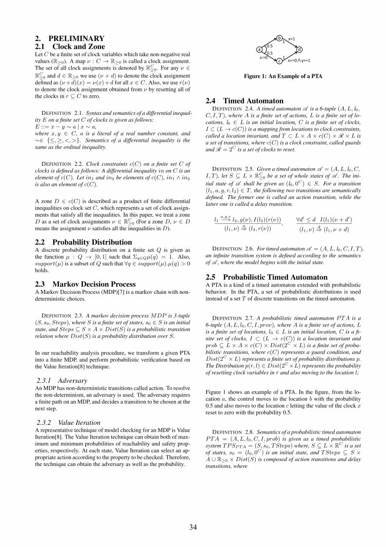
2. PRELIMINARY2.1 Clock and ZoneLet C be a finite set of clock variables which take non-negative realvalues (R≥0). A map ν : C → R≥0 is called a clock assignment.The set of all clock assignments is denoted by R

C≥0. For any ν ∈

RC≥0 and d ∈ R≥0 we use (ν + d) to denote the clock assignment

defined as (ν+d)(x) = ν(x)+d for all x ∈ C. Also, we use r(ν)to denote the clock assignment obtained from ν by resetting all ofthe clocks in r ⊆ C to zero.

DEFINITION 2.1. Syntax and semantics of a differential inequal-ity E on a finite set C of clocks is given as follows:E ::= x− y ∼ a | x ∼ a,where x, y ∈ C, a is a literal of a real number constant, and∼∈ {≤,≥, <,>}. Semantics of a differential inequality is thesame as the ordinal inequality.

DEFINITION 2.2. Clock constraints c(C) on a finite set C ofclocks is defined as follows: A differential inequality in on C is anelement of c(C). Let in1 and in2 be elements of c(C), in1 ∧ in2

is also an element of c(C).

A zone D ∈ c(C) is described as a product of finite differentialinequalities on clock set C, which represents a set of clock assign-ments that satisfy all the inequalities. In this paper, we treat a zoneD as a set of clock assignments ν ∈ R

C≥0 (For a zone D, ν ∈ D

means the assignment ν satisfies all the inequalities in D).

2.2 Probability DistributionA discrete probability distribution on a finite set Q is given asthe function μ : Q → [0, 1] such that Σq∈Qμ(q) = 1. Also,support(μ) is a subset of Q such that ∀q ∈ support(μ).μ(q) > 0holds.

2.3 Markov Decision ProcessA Markov Decision Process (MDP)[7] is a markov chain with non-deterministic choices.

DEFINITION 2.3. A markov decision process MDP is 3-tuple(S, s0, Steps), where S is a finite set of states, s0 ∈ S is an initialstate, and Steps ⊆ S ×A×Dist(S) is a probabilistic transitionrelation where Dist(S) is a probability distribution over S.

In our reachability analysis procedure, we transform a given PTAinto a finite MDP, and perform probabilistic verification based onthe Value Iteration[8] technique.

2.3.1 AdversaryAn MDP has non-deterministic transitions called action. To resolvethe non-determinism, an adversary is used. The adversary requiresa finite path on an MDP, and decides a transition to be chosen at thenext step.

2.3.2 Value IterationA representative technique of model checking for an MDP is ValueIteration[8]. The Value Iteration technique can obtain both of max-imum and minimum probabilities of reachability and safety prop-erties, respectively. At each state, Value Iteration can select an ap-propriate action according to the property to be checked. Therefore,the technique can obtain the adversary as well as the probability.

�

�

�

��

��

��

��

�

Figure 1: An Example of a PTA

2.4 Timed AutomatonDEFINITION 2.4. A timed automaton A is a 6-tuple (A,L, l0,

C, I, T ), where A is a finite set of actions, L is a finite set of lo-cations, l0 ∈ L is an initial location, C is a finite set of clocks,I ⊂ (L → c(C)) is a mapping from locations to clock constraints,called a location invariant, and T ⊂ L × A × c(C) × R × L isa set of transitions, where c(C) is a clock constraint, called guardsand R = 2C is a set of clocks to reset.

DEFINITION 2.5. Given a timed automaton A = (A,L, l0, C,I, T ), let S ⊆ L × R

C≥0 be a set of whole states of A . The ini-

tial state of A shall be given as (l0, 0C) ∈ S. For a transition

(l1, a, g, r, l2) ∈ T , the following two transitions are semanticallydefined. The former one is called an action transition, while thelatter one is called a delay transition.

l1a,g,r−→ l2, g(ν), I(l2)(r(ν))

(l1, ν)a⇒ (l2, r(ν))

,∀d′ ≤ d I(l1)(ν + d′)

(l1, ν)d⇒ (l1, ν + d)

DEFINITION 2.6. For timed automaton A = (A,L, l0, C, I, T ),an infinite transition system is defined according to the semanticsof A , where the model begins with the initial state.

2.5 Probabilistic Timed AutomatonA PTA is a kind of a timed automaton extended with probabilisticbehavior. In the PTA, a set of probabilistic distributions is usedinstead of a set T of discrete transitions on the timed automaton.

DEFINITION 2.7. A probabilistic timed automaton PTA is a6-tuple (A,L, l0, C, I, prov), where A is a finite set of actions, Lis a finite set of locations, l0 ∈ L is an initial location, C is a fi-nite set of clocks, I ⊂ (L → c(C)) is a location invariant andprob ⊆ L × A × c(C) × Dist(2C × L) is a finite set of proba-bilistic transitions, where c(C) represents a guard condition, andDist(2C × L) represents a finite set of probability distributions p.The Distribution p(r, l) ∈ Dist(2C×L) represents the probabilityof resetting clock variables in r and also moving to the location l;

Figure 1 shows an example of a PTA. In the figure, from the lo-cation a, the control moves to the location b with the probability0.5 and also moves to the location c letting the value of the clock xreset to zero with the probability 0.5.

DEFINITION 2.8. Semantics of a probabilistic timed automatonPTA = (A,L, l0, C, I, prob) is given as a timed probabilisticsystem TPSPTA = (S, s0, TSteps) where, S ⊆ L× R

C is a setof states, s0 = (l0, 0

C) is an initial state, and TSteps ⊆ S ×A ∪ R≥0 × Dist(S) is composed of action transitions and delaytransitions, where

34

a) action transitionif a ∈ A and there exists (l, a, g, p) ∈ prob such that g(ν)and I(l′)(r(ν)) for all (r, l′) ∈ support(p), ((l, ν), a, μ) ∈TSteps where for all (l′, ν′) ∈ S

μ(l′, ν′) =∑

r⊆C∧ν′=r(ν)

p(r, l′).

b) delay transitionif d ∈ R≥0, and for all d′ ≤ d, I(l)(ν + d′), ((l, ν), d, μ) ∈TSteps where μ(l, ν + d) = 1.

In this paper, using a location l and a zone D, we describe a set ofsemantic states as (l, D) = {(l, ν) | ν ∈ D}.

DEFINITION 2.9. A path ω with length of n on a timed proba-bilistic system TPSPTA = (S, s0, TSteps, L

′) is denoted as fol-lows.

ω = (l0, ν0)d0,μ0−→ (l1, ν1)

d1,μ1−→ . . .dn−1,μn−1−→ (ln, νn)

, where (li, νi) ∈ S for 0 ≤ i ≤ n and ((li, νi), di, μ) ∈ TSteps∧((li, νi + di), 0, μi) ∈ TSteps ∧ (li+1, νi+1) ∈ support(μi) for0 ≤ i ≤ n− 1.

For model checking of a probabilistic timed automaton, we extracta number of paths and calculate a summation of their occurrenceprobabilities in order to check the probability of satisfying a givenproperty. The important point is that we have to choose a set ofpaths which are compatible with respect to time elapsing.

LEMMA 2.1. If a set Ω of paths on a timed probabilistic systemTPSPTA satisfies the following predicate isCompatible, then allof the paths over Ω are said to be compatible.

isCompatible(Ω) =⎧⎪⎪⎪⎪⎪⎪⎪⎪⎪⎪⎪⎪⎪⎪⎪⎨⎪⎪⎪⎪⎪⎪⎪⎪⎪⎪⎪⎪⎪⎪⎪⎩

true, if ∀i ≤ min(Ω)∧

ωα,ωβ∈Ω

∧ωα �=ωβ

(lαi = lβi ∧ dαi = dβi )

or there exists i ≤ min(Ω) such that∧ωα,ωβ∈Ω

∧ωα �=ωβ

(lαi = lβi ∧ dαi = dβi ∧∧j≤i

(lαj = lβj ∧ dαj= dβj )),

and also∧

Ω′∈2Ω∧Ω′ �=Ω∧|Ω′|≤2

isCompatible(Ω′)

false, otherwise.

In Lemma2.1, we give the predicate isCompatible for a set Ω ofpaths on a timed probabilistic system. In the lemma, we let pathsin Ω be compatible if there is no contradiction with respect to timeelapsing at the branching point of all the paths in Ω, and also ifthe compatibility is kept for every subset of Ω which contains morethan two paths.

2.6 CounterExample-Guided Abstraction Re-finement

2.6.1 General CEGAR TechniqueSince model abstraction sometimes over-approximates an originalmodel, we may obtain spurious CEs which are infeasible on the

��

��

��

��

��

��

��

��

Figure 2: A General CEGAR Technique

��

��

��

��

��

��

��

��

��

��

Figure 3: Our CEGAR Technique for Reachability Analysis ofa Probabilistic Timed Automaton

original model. Paper[5] gives an abstraction refinement frame-work called CEGAR (CounterExample-Guided Abstraction Refine-ment) (Fig.2).

In the algorithm, at the first step (called Initial Abstraction), it gen-erates an initial abstract model. Next, it performs model checkingon the abstract model. In this step, if the model checker reports thatthe model satisfies a given specification, we can conclude that theoriginal model also satisfies the specification, because the abstractmodel is an over-approximation of the original model. If the modelchecker reports that the model does not satisfy the specification,however, we have to check whether the CE detected is spurious ornot in the next step (called Simulation). In the Simulation step, ifwe find that the CE is valid, we stop the loop. Otherwise, we haveto refine the abstract model to eliminate the spurious CE, and repeatthese steps until valid output is obtained.

2.6.2 CEGAR Technique for a Timed AutomatonIn [6], we have proposed the abstraction refinement technique fora timed automaton based on the framework of CEGAR. In this ap-proach, we remove all the clock attributes from a timed automa-ton. If a spurious CE is detected by model checking on an abstractmodel, we transform the transition relation on the abstract model sothat the model behaves correctly even if we don’t consider the clockconstraints. Such transformation obviously represents the differ-ence of behavior caused by the clock attributes. Therefore, the fi-nite number of application of the refinement algorithm enables usto check the given property without the clock attributes. Since ourapproach does not restore the clock attributes at the refinement step,the abstract model is always a finite transition system without theclock attributes.

3. PROPOSED APPROACHIn this section, we will present our abstraction refinement techniquefor a probabilistic timed automaton. In the technique, we use theabstraction refinement technique for a timed automaton proposed

35

�

�

�

��

��

�

��

Figure 4: An Initial Abstract Model

in [6]. In addition, we resolve the compatibility problem shown inSec.2.5 by performing a backward simulation technique and gen-erating additional location to distinguish the required condition forevery incompatible path. Figure 3 shows our abstraction refinementframework. As shown in the figure, we add another flow where weresolve the compatibility problem.

Our abstraction requires a probabilistic timed automaton PTA anda property to be checked as its inputs. The property is limited by thePCTL formula P<p[true U err]. The formula represents a propertythat the probability of reaching to states where err (which meansan error condition in general) is satisfied, is less than p.

3.1 Initial AbstractionThe initial abstraction removes all the clock attributes from a givenprobabilistic timed automaton as well as the technique in The gen-erated abstract model over-approximates the original probabilistictimed automaton.

DEFINITION 3.1. For a given probabilistic timed automatonPTA = (A,L, l0, C, I, prob), a markov decision process

ˆMDPPTA = (S, s0, ˆSteps) is produced as its abstract model,where S = L, s0 = l0, and ˆSteps = { (s, a, p) | (s, a, g, p) ∈prob }

Figure 4 shows an initial abstract model for the PTA shown in Fig.1As shown in the figure, the abstract model is just an MDP where allof the clock constraints are removed though we keep a set of clockreset as a label of transitions.

3.2 Model CheckingIn model checking, we apply Value Iteration[8] into the markovdecision process obtained by abstraction and calculate a maximumreachability probability. Also, it decides an action to be chosen atevery state as an adversary. If the obtained probability is less than p,we can terminate the CEGAR loop and conclude that the propertyis satisfied.

Although Value Iteration can calculate a maximum reachabilityprobability, it cannot produce concrete paths used for the proba-bility calculation. To obtain the concrete paths, we use an approachproposed in [9] which can produce CE paths for PCTL formulas.The approach translates a probabilistic automaton into a weighteddigraph. And we can obtain at most k paths by performing k-shortest paths search on the graph.

DEFINITION 3.2. A path ω on an abstract model ˆMDPPTA =(S, s0, ˆSteps) for PTA = (A,L, l0, C, I, prob) is given as fol-lows,

ω = s0a0,p0,r0−→ s1

a1,p1,r1−→ . . .an−1,pn−1,rn−1−→ sn

� � �

��

��

��

��

�� !�

��"��#��$��%$��"��

��

� � ��

� � ��

�� !��

� ��

��

��

��

��

��

��

��

��

��& ��

��"��#��$��%$��"��

Figure 5: Products of zones obtained by Forward and Back-ward Simulation

, where si ∈ S for 0 ≤ i ≤ n and (si, ai, pi) ∈ ˆSteps ∧(ri, si+1) ∈ support(pi) for 0 ≤ i ≤ n− 1.

As defined in Def. 3.2, we associate a set r of clock reset with apath on an abstract model in order to show the difference of r overthe probabilistic distribution p.

For the abstract model shown in Fig.4, Value Iteration outputs 1.0as the probability that it reaches to the state d from the state a. Onthe other hand, k-shortest paths search (k ≥ 2) detects two paths

ωα = aτ,0.5,{}−→ b

τ,1.0,{}−→ d and ωβ = aτ,0.5,{x:=0}−→ c

τ,1.0,{}−→ d,where τ represents a label for transitions with no label in the figure.

3.3 SimulationSimulation checks whether all the paths obtained by k-shortest pathssearch are feasible or not on the original probabilistic timed au-tomaton. We use the simulation algorithm proposed in [6] If thereis at least one path which is infeasible on the original PTA, we pro-ceed to the abstraction refinement step.

3.4 Abstraction RefinementIn this step, we refine the abstract model so that the given spuri-ous CE also becomes infeasible on the refined abstract model. Wecan use the algorithm proposed in [6]. Since the algorithm of [6]performs some operations on transitions of a timed automaton, wereplace such operations by those on probability distributions of aprobabilistic timed automaton.

3.5 Compatibility CheckingWhen all the paths obtained by k-shortest paths search are feasibleand a summation of occurrence probabilities of them is greater thanp, we also have to check whether all the paths are compatible or not.In this compatibility checking step, at each location of the paths, wehave to obtain a condition (zone) which is reachable from the initialstate and also reachable to the last state along with the path. Next,we check the compatibility of such conditions among all paths. Toobtain such conditions, we have to perform both forward simulationshown in Sec. 3.3 and backward simulation for each path, andmerge the results. For the result of forward simulation, we canreuse the result obtained in the Simulation step. Then we check thecompatibility based on Lemma 2.1. Paper[10] shows the algorithmof compatibility checking in detail. In the algorithm, we check thecompatibility of such products of zones at every location of thepaths.

Figure 5 shows the products of zones obtained by both forward andbackward simulation for two paths ωα and ωβ in Sec.3.2. For thepath ωα, the product zone at a is given as Dωα

c,0 = (x == y ∧ x <

36

Table 1: Experimental ResultDigital Clocks[3] Proposed Approach

D(μs) p Result T ime(s) State MEM(MB) Result T ime(s) Loop State Heap(MB)

51.09×10−1 false 20.90 297,232 10.2 false 4.19 10 37 8.0

3.28×10−1 true 20.89 297,232 10.2 true 3.60 9 36 8.0

101.26×10−2 false 54.80 685,232 21.7 false 8.16 19 134 8.0

3.79×10−2 true 54.82 685,232 21.7 true 6.57 15 115 8.0

201.85×10−4 false 176.93 1,461,232 41.0 false 1186.08 47 477 64.0

5.56×10−4 true 177.46 1,461,232 41.0 true 31.32 32 435 8.0

� ��

��

�'

�'

�(

�(

��

��&��

��

�& ��

�)��*��) ��*

�)��&��*��)�& ��*

��

��

��

�

�

��

��

��

��

��

��

��

Figure 6: A Transformed PTA

1), which means a zone which is reachable from the initial stateand also can move to d. Similarly, for the path ωβ , the product

zone is given as Dωβ

c,0 = (x == y ∧ y > 1). Since Dωα

c,0 and Dωβ

c,0

contradict each other, we can conclude that the paths ωα and ωβ

are incompatible each other.

3.6 Model TransformationWhen the compatibility check procedure decides a given set Ω ofpaths is incompatible at i-th location, our proposed algorithm re-solves the incompatibility by refining behaviors from the i-th lo-cation. Our algorithm uses Dω

c which is a product of results offorward and backward simulation for a path ω ∈ Ω. It duplicateslocations which are reachable from the zone Dω

c,i by an action as-sociated with the i-th distribution pi. Also it constructs transitionrelations so that the transformation becomes equivalent transfor-mation. For example, transition relations from a duplicated loca-tion are duplicated if the relations are executable from the invari-ant associated with the duplicated location. Detailed Algorithms totransform the model are given in [10].

Figure 6 shows the transformed PTA by applying the model trans-formation procedure for the paths ωα and ωβ . The locations b1

and c1 are duplicated locations based on the path ωα and the zone

Dωβ

c,0 = (x == y ∧ x < 1) on the location a. We associate invari-

ants to b1 and c1 based on zones which are reachable from Dωβ

c,0

through transitions from a to b, and from a to c, respectively. Also,we duplicate a transition from b to d as the transition from b1 to dbecause the transition is feasible from the invariant of b1. On theother hand, we do not duplicate a transition from c to d because thetransition is not feasible from the invariant of c1. Similarly, loca-tions b2 and c2 are duplicated locations based on the path ωβ and

the zone Dωβ

c,0 . Locations b3 and c3 are generated as complementsof the invariant associated with each duplicated location in order topreserve the equivalence.

By transforming the original PTA in such a way, if we remove allclock constraints from the model in Fig.6, Value Iteration on its

abstract model outputs 0.5 as the maximum probability.

4. EXPERIMENTSWe have implemented a prototype of our proposed approach withJava, and performed some experiments. Though the prototype cancheck the compatibility of a given set of paths, currently it cannotdeal with the model transformation.

The prototype performs k-shortest paths search and simulation con-currently in order to reduce execution time. By implementing thealgorithms concurrently, we have not to wait until all of k paths aredetected, i.e. if a path is detected by the k-shortest paths searchalgorithm, we can immediately apply simulation and (if needed)abstraction refinement procedures. Also, our prototype continuesthe k-shortest search algorithm when a spurious CE is detected andthe refinement algorithm is applied. If other paths which do notoverlap with the previous spurious CEs, are detected, we can ap-ply simulation and refinement algorithms to it again. This helps usreduce the number of CEGAR loop.

4.1 Goal of the ExperimentsThe goal of this experiment is to check that our approach, whichalso searches a CE, is performed within realistic time. In this ex-periment, we evaluated the performance of our proposed approachwith regard to execution time, memory consumption, and quali-ties of obtained results. As a target for comparison, we chose theapproach of Digital Clocks[3], which is considered as a basic ap-proach, where they approximate clock evaluations of a PTA by in-teger values.

4.2 ExampleWe used a case study of the FireWire Root Contention Protocol[11]as an example for this experiment. This case study concerns theTree Identify Protocol of the IEEE 1394 High Performance SerialBus (called “FireWire”) which takes place when a node is addedor removed from the network. In the experiment, we checked theprobability that a leader is not selected within a given deadline. Theprobabilistic timed automaton for the example is composed of twoclock variables, 11 locations, and 24 transitions.

4.3 Procedure of the ExperimentsIn this experiment, we checked the property that “the probabilitythat a leader cannot be elected within a given deadline is less thanp.” We considered three scenarios where the parameter deadlineis 5, 10, 20 μs, respectively. Also, for each scenario, we conductedtwo experiments where the value of p is 1.5 times as an approximatevalue of the maximum probability obtained by the Digital Clocksapproach[3] and a half of it, respectively. In the proposed approach,we searched at most 5000 paths by letting the parameter k of the k-shortest paths search algorithm be 5000. For evaluation of existingapproach, we used the probabilistic model checker PRISM[12].

37

Table 2: Analysis of Counter Example PathsD(μs) p Path Probability CC(ms)

5 1.0938×10−1 7 1.2500×10−1 0.7

10 1.2635×10−2 43 1.2695×10−2 5.9

20 1.8500×10−4 2534 1.8501×10−4 296.9

The experiments were performed under Intel Core2 Duo 2.33 GHz,2GB RAM, and Fedora 12 (64bit).

4.4 Results of the ExperimentsThe results are shown in Table 1. The column of D means the valueof deadline. For each approach, columns of Results, T ime,and States show the results of model checking, execution time ofwhole process, and the number of states constructed, respectively.The column MEM in the columns of the Digital Clocks shows thememory consumption of PRISM. The columns Loop and Heap inthe columns of the proposed approach show the number of CEGARloops executed and the maximum heap size of the Java Virtual Ma-chine (JVM) which executes our prototype, respectively.

Table 1 shows that for all cases we can dramatically reduce thenumber of states and obtain correct results. Moreover, we can re-duce the execution time more than 80 percent except for the casewhen deadline = 20μs and p = 1.85 × 10−4. In this case, how-ever, the execution time drastically increases.

Table 2 shows the results of analysis of CE paths obtained whenthe results of model checking are false. The columns of Path,Probability and CC show the number of CE paths, the summationof occurrence probability of them, and execution time for compati-bility checking, respectively. For this example, the obtained sets ofCE paths are compatible in every case.

4.5 DiscussionFrom the results shown in Table 1, we can see that our proposedapproach is efficient with regard to both execution time and thenumber of states. Especially, the number of states decrease dramat-ically. The execution time is also decreased even though we per-form model checking several times shown in the column of Loop.

On the other hand, in the case when deadline = 20μs and p =1.85 × 10−4, the execution time increases drastically. We thinkthat as shown in Table 2 we have to search 2534 paths and thiscauses the increase of execution time especially for k-shortest pathssearch. A more detailed analysis shows that the execution time fork-shortest paths search accounts for 1123 seconds of total execu-tion time of 1186 seconds. Also, the results shows that the JVMneeds 64MB as its heap size in this case. This is because com-patibility checking for 2534 of paths needs a large amount of thememory. From the results, we have to resolve a problem of thescalability when the number of candidate paths for a CE becomeslarge.

5. CONCLUSIONThis paper proposed the abstraction refinement technique for a prob-abilistic timed automaton by extending the existing abstraction re-finement technique for a timed automaton. The main contributionof this work is generation of a CE. Also, the experimental resultsshow the efficiency of our technique compared to one of existingapproaches.

Future work includes completion of implementation. General DBMdoes not support not operator[13]; so we have to investigate effi-cient algorithms for the not operator.

AcknowledgmentsThis work is being conducted as a part of Stage Project, the Devel-opment of Next Generation IT Infrastructure, supported by Min-istry of Education, Culture, Sports, Science and Technology, aswell as Grant-in-Aid for Scientific Research C(21500036), as wellas grant from The Telecommunications Advancement Foundation.

6. REFERENCES[1] E. M. Clarke, O. Grumberg, and D. A. Peled, editors. Model

checking. MIT Press, 1999.

[2] M. Kwiatkowska, G. Norman, J. Sproston, and F. Wang.Symbolic model checking for probabilistic timed automata.Information and Computation, 205(7):1027–1077, 7 2007.

[3] M. Kwiatkowska, G. Norman, and J. Sproston. Performanceanalysis of probabilistic timed automata using digital clocks.Int. Journal on Formal Methods in System Design,29(1):33–78, 7 2006.

[4] M. Kwiatkowska, G. Norman, and D. Parker. Stochasticgames for verification of probabilistic timed automata. InProc. of the 7th Int. Conf. on Formal Modeling and Analysisof Timed Systems (FORMATS’09), volume 5813 of LNCS,pages 212–227, 9 2009.

[5] E. M. Clarke, O. Grumberg, S. Jha, Y. Lu, and V. Helmut.Counterexample-guided abstraction refinement for symbolicmodel checking. Journal of the ACM, 50(5):752–794, 2003.

[6] T. Nagaoka, K. Okano, and S. Kusumoto. An abstractionrefinement technique for timed automata based oncounterexample-guided abstraction refinement loop. IEICETransactions on Information and Systems,E93-D(5):994–1005, 5 2010.

[7] C. Derman, editor. Finite-State Markovian DecisionProcesses. New York: Academic Press, 1970.

[8] D. P. Bertsekas. Dynamic programming and optimal control.Athena Scientific, 1995.

[9] H. Aljazzar and S. Leue. Directed explicit state-space searchin the generation of counterexamples for stochastic modelchecking. IEEE Transactions on Software Engineering,36(1):37–60, 1 2010.

[10] A. Ito, T. Nagaoka, K. Okano, and S. Kusumoto.Reachability analysis for probabilistic timed system based ontimed abstraction refinement technique (in japanese). InIEICE Technical Report, volume 109, pages 85–90, 3 2010.

[11] M. Kwiatkowska, G. Norman, and J. Sproston. Probabilisticmodel checking of deadline properties in the ieee1394firewire root contention protocol. Formal Aspects ofComputing, 14(3):295–318, 4 2003.

[12] A. Hinton, M. Kwiatkowska, G. Norman, and D. Parker:.PRISM: A tool for automatic verification of probabilisticsystems. In Proc. of the 12th Int. Conf. on Tools andAlgorithms for the Construction and Analysis of Systems(TACAS’06), volume 3920, pages 441–444, 2006.

[13] A. David, J. Hakansson, K G. Larsen, and P. pettersson.Model checking timed automata with priorities using dbmsubtraction. In Proc. of the 4th Int. Conf. on FormalModelling and Analysis of Timed Systems, pages 128–142,2006.

38

Fault-prone Module Prediction Using Contents ofComment Lines

Osamu MizunoKyoto Institute of Technology

Matsugasaki Goshokaido-cho, Sakyo-kuKyoto 606-8585, [email protected]

Yukinao HirataKyoto Institute of Technology

Matsugasaki Goshokaido-cho, Sakyo-kuKyoto 606-8585, Japan

[email protected]

ABSTRACTComment lines in the software source code include descriptionsof codes, usage of codes, copyrights, unused codes, comments,and so on. From the viewpoint of fault-prone module prediction,comment lines may have useful information for faulty modules aswell as in code lines. In fault-proneness filtering approach, whichwe have been proposed based on text filtering technique, commentlines and code lines in a source code modules are regarded as textwithout any distinction. For better prediction results of fault-pronemodules, the effects of the comment lines on prediction should beinvestigated. This study conducts experiments using Eclipse datasets to reveal the effects of comment lines on the fault-pronenessfiltering. The result of experiments was somehow unexpected: pre-diction using comment lines shows better recall and precision thanthat of code lines.

Categories and Subject DescriptorsD.2.5 [Software Engineering]: Testing and Debugging; D.2.7 [SoftwareEngineering]: Distribution, Maintenance, and Enhancement; D.2.9[Software Engineering]: Management

General TermsMeasurement

1. INTRODUCTIONFault-prone prediction is one of the most mature areas of soft-ware engineering. The prediction of faulty software modules isimportant for both the reduction of development cost and the as-surance of software quality. Much research has been conductedso far [1, 3, 4, 6–13, 16]. Most research used some kind of soft-ware metrics, such as program complexity, size of modules, object-oriented metrics, etc., and constructed mathematical models to cal-culate fault-proneness. This approach is usually based on a hy-pothesis that the more complex module the more bugs. However,such a hypothesis is not always true. For example, although manyif-sentences increase program complexity,

We thus tried to break through the conventional fault-prone predic-

tion by introducing a text-mining technique. This paper introducesa new idea for fault-prone module detection. The idea is inspiredfrom a spam e-mail filtering technique. Spam filters are usually im-plemented as a generic text discriminator. We thus tried to apply ageneric text discriminator to the fault-prone detection. We call ourapproach “fault-prone filtering.” In fault-prone filtering, we con-sider a software module as an e-mail message, and assume that allof the software modules belong to either fault-prone(FP) modulesor not-fault-prone(NFP) modules. After learning of existing FP andNFP modules, we can classify a new module into either FP or NFPby applying a spam filter. One advantage of such a statistical ap-proach is that we do not have to investigate source code modules indetail. We do not measure any metrics explicitly, but implicitly ourapproach measures only one metric: frequency of tokens found inthe source code.

Although we have confirmed usefulness of our approach, there areseveral remaining issues. One issue is effect of comment lines.Previous implementation of fault-prone filtering did not distinguishthe comment lines and code lines. This is because the source codemodule is passed into text filter without any modification. How-ever, since code lines and comment lines have different roles insource code modules, we need to consider such difference in thefault-prone filtering. We expect to improve the prediction accuracyof fault-prone filtering by using information obtained from com-ment lines.

To do so, we conducted an experiment to confirm the effect of com-ment lines in the source code modules to the fault-prone filtering.The result of experiment showed that comment lines have almostthe same capability as code lines to predict fault-prone modules.

2. OBJECTIVE2.1 Fault-prone module filteringThe basic idea of fault-prone filtering is inspired by spam mail fil-tering. In spam e-mail filtering, the spam filter first trains both spamand ham e-mail messages from the training data set. Then, an in-coming e-mail is classified into either ham or spam by the spamfilter.

This framework is based on the fact that spam e-mail usually in-cludes particular patterns of words or sentences. From the view-point of source code, a similar situation usually occurs in faultysoftware modules. That is, similar faults may occur in similar con-texts. We thus guessed that similar to spam e-mail messages, faultysoftware modules have similar patterns of words or sentences. Toobtain such features, we adopted a spam filter in fault-prone mod-ule prediction.

39

Intuitively speaking, we try to introduce a new metric as a fault-prone predictor. The metric is “frequency of particular words”. Indetail, we do not treat a single word, but use combinations of wordsfor the prediction. Thus, the frequency of a certain length of wordsis the only metric used in our approach.

We then try to apply a spam filter to identification of fault-pronemodules. We named this approach as “fault-prone filtering”. Thatis, a learner first trains both faulty and non-faulty modules. Then,a new module can be classified into fault-prone or not-fault-proneusing a classifier.

In this study, we define a software module as a Java class file.

2.2 Effect of comment linesIn this paper, we call “comments” in the source code module ascomment lines, and call other lines as “code lines”.

Code lines describe a list of operations that developers would liketo realize on computers. Comment lines include descriptions ofcode lines, usage of methods or modules. Code lines are written ina specific programming language, but comment lines are written ina free form.

Previous implementation of fault-prone filtering did not distinguishthe comment lines and code lines. This is because the source codemodule is passed into text filter without any modification. How-ever, since code lines and comment lines have different roles insource code modules, we need to consider such difference in thefault-prone filtering.

For example, comments are usually placed near the difficult codes.Therefore, learning the contents of comment lines may be useful toidentify the bug-related part in modules. We expect to improve theprediction accuracy of fault-prone filtering by using comment lineseffectively.

3. IMPLEMENTATION OF FAULT-PRONEFILTER

In the previous studies [14,15], we used a ready-made open-sourcetext classifier, CRM114 [19]. However, use of ready-made softwarehides essential information in experiments. We thus implement atext classifier from scratch for this experiment.

3.1 TokenizationFirst of all, inputs of fault-prone filter must be tokenized. Codelines are tokenized by the Java syntax scanner as follows:

1. Strings with alphabets, numeric characters, and period

2. Operators in Java language

3. Strings with single quotations

4. Strings with double quotations

Other characters, spaces, commas, braces, colons, semicolons, andso on, are used as a separator to make tokens.

As for the comment lines, tokenization is done by similar mannerwith the case of code lines. However, since it is difficult to deter-mine the end of quoted strings in comment lines, we treat single

Comment lines in faulty modules

Faulty

Comment lines in non-faulty

modules

Non-faulty

Faulty commentcorpus

Non-faulty commentcorpus

Tokenize and learn

Tokenize and learn

Mftcom Mnf

com

Figure 1: Learning procedure

and double quotations as a separator in the comment lines. Con-sequently, a code piece output("Hello, world!"); is to-kenized into 2 tokens, “output” and “"Hello, world"”, incode lines, but is tokenized into 3 tokens, “output”, “Hello”,and “world” in comment lines.

3.2 Learning algorithmThe algorithm of learning and classification is the same as that of[5].

Step 1 Tokens are extracted from faulty and non-faulty modules.The number of occurrence for each token in faulty and non-faulty modules are counted. For a given token t, the follow-ing two hash functions can be defined:

• nonfaulty(t): The occurrence of token t in all non-faulty modules.

• faulty(t): The occurrence of token t in all faulty mod-ules.

Step 2 We construct a hash table to obtain the probability, Pft|t,by equation (1) that a module that includes the token t isfaulty. Here, Nnf denotes the number of non-faulty modulesand Nft denotes the number of faulty modules. We call thishash table as a corpus.

rnf = min

„1,

2× nonfaulty(t)

Nnf

«

rft = min

„1,

faulty(t)

Nft

«

Pft|t = max

„0.01, min

„0.99,

rft

rnf + rft

««(1)

3.3 Classification algorithmThe classification process is also based on Graham’s algorithm [5].

40

A newJava source code

module

Comment lines in a module

Code linesin a module

Classification Classification

Faulty commentcorpus

Non-faulty commentcorpus

Faulty codecorpus

Non-faulty code

corpus

Probability to faulty

Probability to faulty

Mcom Mcode

M

Figure 2: Classification procedure

Step 1 For a new module, distinct tokens are extracted. In thisstudy, we use all extracted tokens. Here, we count the num-ber of tokens, n, for the next step1.

Step 2 According to the equation (2), the probability Pft is calcu-lated. We determine whether a module is fault-prone or not.If Pft ≥ 0.9, the module is determined as fault-prone.

Pft =

Qni=1 Pft|tiQn

i=1 Pft|ti+

Qni=1(1− Pft|ti

)(2)

To both comment lines and code lines, we separately apply thisclassification algorithm. Intuitive description of the classificationprocedure is shown in Figure 2.

4. EXPERIMENT4.1 Target projectIn order to conduct experiments, we prepare a data set obtainedfrom Eclipse project by Zimmermann [2,20], which is called promise-2.0a data set. In the data set, 31 complexity metrics as well as thenumber of pre- and post-release faults are defined and collected.Although promise-2.0a includes metrics collected from both filesand packages, we used the metrics from files for this study. One ofadvantages to use promise-2.0a from Eclipse is that it is publicly

1We can use a limited number of tokens here. To do so, amongthose extracted tokens, most characteristic n tokens, t1 · · · tn aredetermined. In more detail, Cx = abs(0.5 − Pft|tx) is calculatedfor each token tx, and we select n tokens with the largest Cxs bydescending order. For calculation of Cx, if a token t is a never seenone, we assume that Pft|t = 0.4. Based on the pre-experiment, wefound that the prediction performance does not differ if we use, forexample, 20 characteristic tokens. But for simplicity, we used alltokens in this experiment.

Table 1: Target projectsProject Eclipse

Version 2.0 2.1 3.0

Number of modules 6,729 7,888 10,593

Number of faulty 975 854 1,568modules (14.5%) (10.8%) (14.8%)

Number of non- 5,754 7,034 9,025faulty modules (85.5%) (89.2%) (85.2%)

Total lines of code 1,267,350 1,564,872 2,098,034

Comment lines 475,486 577,033 788,055(37.5%) (36.9%) (37.6%)

Code lines 791,864 987,839 1,309.979(62.5%) (63.1%) (62.4%)

Table 2: Classification result matrixClassified

non-fault-prone fault-prone

Actual non-faulty True negative (TN) False positive (FP)faulty False negative (FN) True positive (TP)

available on the Web. Many researchers can use the same data setand compare their approaches. The data set includes the values ofsoftware complexity metrics shown and fault data collected by theSZZ algorithm [18] for each class file, that is, software modules.The data is obtained from Eclipse version 2.0, 2.1, and 3.0. Thenumber of modules in Eclipse 2.0, 2.1 and 3.0 are 6,729, 7,888 and10,593, respectively.

4.2 Evaluation measuresTable 2 shows a classification result matrix. True negative (TN)shows the number of modules that are classified as non-fault-prone,and are actually non-faulty. False positive (FP) shows the numberof modules that are classified as fault-prone, but are actually non-faulty. On the contrary, false negative shows the number of mod-ules that are classified as non-fault-prone, but are actually faulty.Finally, true positive shows the number of modules that are classi-fied as fault-prone which are actually faulty.

In order to evaluate the results, we prepare two measures: recall,precision. Recall is the ratio of modules correctly classified asfault-prone to the number of entire faulty modules Recall is definedby equation (3).

Recall =TP

TP + FN(3)

Precision is the ratio of modules correctly classified as fault-proneto the number of entire modules classified fault-prone. Precision isdefined by equation (4).

Precision =TP

TP + FP(4)

Accuracy is the ratio of correctly classified modules to the entiremodules. Accuracy is defined by equation (5).

Accuracy =TP + TN

TN + TP + FP + FN(5)

Since recall and precision are in the trade-off, F1-measure is usedto combine recall and precision. F1-measure is defined by equation

41

Java source codemodules

FaultyJava source code

modules

FaultyNon-faulty

Java source codemodules

Non-faulty

Comment lines in faulty modules

Faulty

Code linesin faulty modules

Faulty

Comment lines in non-faulty

modules

Non-faulty

Code linesin non-faulty

modules

Non-faulty

M

Mft Mnf

Mnfcom Mnf

codeMft

codeMftcom

Figure 3: Getting modules

(6).

F1 =2× recall× precision

recall + precision(6)

In this definition, recall and precision are evenly weighed.

4.3 Application to EclipseIn this section, we describe a procedure of experiments.

We obtained the source code modules from tar archives of corre-sponding Eclipse versions. We can define faulty and non-faultysource code modules by the metric “post-release failure (post)” inpromise-2.0a. If post > 0, a module is faulty; otherwise non-faulty. Based on the faulty/non-faulty information, we divide sourcecode modules into “faulty” and “non-faulty”, represented ft andnf , respectively. Moreover, we separate a module into code andcomment lines for each source code module. This procedure isshown in Figure 3.

Here, let Mcode and Mcom be code lines and comment lines ex-tracted from a module M , respectively. In the classification withcode lines, we use only Mcode as training and test data. Similarly,we use only Mcom in the classification with comment lines.

The following procedure was conducted in this experiment:

1. For the learning step, we first pick up a version of Eclipseproject as a training data set. We then divide the trainingdata set into faulty and non-faulty. For each faulty module,Mft

code is extracted and conducted learning for a faulty code

corpus. Similarly, Mftcom is extracted and learnt in a faulty

comment corpus. For non-faulty modules, the same proce-dure for Mnf

code and Mnfcom is performed.

2. For the classification step, we pick up the other version ofEclipse project as a testing data set. The, the testing dataset is applied to the classification procedure. For each mod-ule in the testing data set, Mcode and Mcom are extracted.

Table 3: Result of prediction: (comment, 2.0, 2.1)Prediction


Actual not faulty 5,952 1,082faulty 508 346

Table 4: Result of prediction: (code, 2.0, 2.1)Prediction









By using code and comment corpuses, Mcode and Mcom areclassified.

In this experiment, we use versions 2.0 and 2.1 for training and ver-sions 2.1 and 3.0 for testing, since it is natural to use older versionfor training and newer version for testing. These training pairs areused for different targets: code lines or comment lines. We thusprepare six experiment 3-tuples denoted by (target, training, test-ing): (code, 2.0, 2.1), (comment, 2.0, 2.1), (code, 2.0, 3.0), (com-ment, 2.0, 3.0), (code, 2.1, 3.0), and (comment, 2.1, 3.0).

The results of six prediction experiments are shown in Tables 3 –8.

4.4 Result of experimentA summary of experimental results are shown in Table 9. Boldfigures show the best result. We can find following three findingsfrom Table 9:

1. Predicted results with comment lines have better F1’s thanthat of code lines.






Actual not faulty 7,883 1,142faulty 1,133 435

42

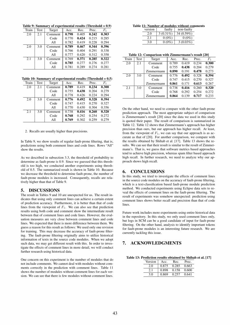
Table 9: Summary of experimental results (Threshold = 0.9)Train Test Target Acc. Rec. Prec. F1

2.0 2.1 Comment 0.798 0.405 0.242 0.303Code 0.770 0.424 0.215 0.285All 0.782 0.419 0.228 0.294

2.0 3.0 Comment 0.789 0.467 0.344 0.396Code 0.766 0.404 0.291 0.338All 0.777 0.420 0.312 0.358

2.1 3.0 Comment 0.769 0.371 0.285 0.322Code 0.785 0.277 0.276 0.277All 0.781 0.289 0.274 0.281

Table 10: Summary of experimental results (Threshold = 0.5)Train Test Target Acc. Rec. Prec. F1

2.0 2.1 Comment 0.789 0.419 0.234 0.300Code 0.755 0.438 0.204 0.279All 0.778 0.426 0.224 0.294

2.0 3.0 Comment 0.776 0.492 0.328 0.394Code 0.747 0.415 0.270 0.327All 0.770 0.430 0.304 0.356

2.1 3.0 Comment 0.738 0.416 0.260 0.320Code 0.768 0.292 0.254 0.272All 0.769 0.302 0.259 0.279

2. Recalls are usually higher than precisions.

In Table 9, we show results of regular fault-prone filtering, that is,predictions using both comment lines and code lines. Rows “All”show the results.

As we described in subsection 3.3, the threshold of probability todetermine as fault-prone is 0.9. Since we guessed that this thresh-old is too high, we conducted another experiments using thresh-old of 0.5. The summarized result is shown in Table 10. Becausewe decrease the threshold to determine fault-prone, the number offault-prone modules is increased. Consequently, recalls are rela-tively higher than that of Table 9.

5. DISCUSSIONSThe result in Tables 9 and 10 are unexpected for us. The result in-dicates that using only comment lines can achieve a certain extentof prediction accuracy. Furthermore, it is better than that of codelines from the viewpoint of F1. We can also see that predictionresults using both code and comment show the intermediate resultbetween that of comment lines and code lines. However, the eval-uation measures are very close between comment lines and codelines. We expected that there is more difference between them. Weguess a reason for this result as follows: We used only one revisionfor training. This may decrease the accuracy of fault-prone filter-ing. The fault-prone filtering originally aims to utilize historicalinformation of texts in the source code modules. When we adoptsuch data, we may get different result with this. In order to inves-tigate the effects of comment lines in more detail, we will conductfurther research using historical data.

One concern on this experiment is the number of modules that donot include comments. We cannot deal with modules without com-ments correctly in the prediction with comment lines. Table 11shows the number of modules without comment lines for each ver-sion. We can see that there is few modules without comment lines.

Table 11: Number of modules without commentsversion faulty non-faulty

2.0 3 (0.31%) 34 (0.59%)

2.1 0 (0%) 0 (0%)

3.0 0 (0%) 3 (0.03%)

Table 12: Comparison with Zimmermann’s result [20]Train Test Target Acc. Rec. Prec. F1

2.0 2.1 Comment 0.789 0.419 0.234 0.300Code 0.755 0.438 0.204 0.279

Zimmermann 0.890 0.191 0.478 0.273

2.0 3.0 Comment 0.776 0.492 0.328 0.394Code 0.747 0.415 0.270 0.327

Zimmermann 0.861 0.171 0.613 0.267

2.1 3.0 Comment 0.738 0.416 0.260 0.320Code 0.768 0.292 0.254 0.272

Zimmermann 0.864 0.139 0.717 0.233

On the other hand, we need to compare with the other fault-proneprediction approach. The most appropriate subject of comparisonis Zimmermann’s result [20] since the data we used in this studyis quoted their paper. The result of comparison is summarized inTable 12. Table 12 shows that Zimmermann’s approach has higherprecision than ours, but our approach has higher recall. At least,from the viewpoint of F1, we can say that our approach is as ac-curate as that of [20]. For another comparison, we compare withthe results obtained by Shihab et al. [17]. Table 13 shows the re-sults. We can see that their result is similar to the result of Zimmer-mann’s. That is, we guess that software metrics based approachestend to achieve high precision, whereas spam filter based approachhigh recall. In further research, we need to analyze why our ap-proach shows high recall.

6. CONCLUSIONSIn this study, we tried to investigate the effects of comment linesin the source code modules on the accuracy of fault-prone filtering,which is a text-classification based fault-prone module predictionmethod. We conducted experiments using Eclipse data sets to re-veal the effects of comment lines on the fault-prone filtering. Theresult of experiments was somehow unexpected: prediction usingcomment lines shows better recall and precision than that of codelines.

Future work includes more experiments using entire historical datain the repository. In this study, we only used comment lines only,but logs in SCM can be a good candidate of input for fault-pronefiltering. On the other hand, analysis to identify important tokensfor fault-prone modules is an interesting future research. We arecurrently tackling this issue.

7. ACKNOWLEDGMENTS

Table 13: Prediction results obtained by Shihab et al. [17]Version Acc. Rec. Prec.

2.0 0.875 0.285 0.663

2.1 0.898 0.158 0.600

3.0 0.869 0.257 0.641

43

This research is partially supported by the Japan Ministry of Edu-cation, Science, Sports and Culture, Grant-in-Aid for Young Scien-tists (B), 20700025, 2008–2010.

8. REFERENCES[1] P. Bellini, I. Bruno, P. Nesi, and D. Rogai. Comparing

fault-proneness estimation models. In Proc. of 10th IEEEInternational Conference on Engineering of ComplexComputer Systems, pages 205–214, 2005.

[2] G. Boetticher, T. Menzies, and T. Ostrand. PROMISERepository of empirical software engineering datarepository. http://promisedata.org/, West Virginia University,Department of Computer Science, 2007.

[3] L. C. Briand, W. L. Melo, and J. Wust. Assessing theapplicability of fault-proneness models acrossobject-oriented software projects. IEEE Trans. on SoftwareEngineering, 28(7):706–720, 2002.

[4] G. Denaro and M. Pezze. An empirical evaluation offault-proneness models. In Proc. of 24th InternationalConference on Software Engineering, pages 241–251, 2002.

[5] P. Graham. Hackers and Painters: Big Ideas from theComputer Age, chapter 8, pages 121–129. O’Reilly Media,2004.

[6] L. Guo, B. Cukic, and H. Singh. Predicting fault pronemodules by the dempster-shafer belief networks. In Proc. of18st International Conference on Automated SoftwareEngineering, pages 249–252, 2003.

[7] T. M. Khoshgoftaar and E. B. Allen. Logistic regressionmodeling of software quality. International Journal ofReliability, Quality and Safety Engineering, 6(4):303–317,1999.

[8] T. M. Khoshgoftaar and E. B. Allen. Controlling overfittingin classification tree models of software quality. EmpiricalSoftware Engineering, 6(1):59–79, 2001.

[9] T. M. Khoshgoftaar, E. B. Allen, and J. Deng. Usingregressin trees to classify fault-prone software modules.IEEE Trans. on Reliability, 51(4):455–462, 2002.

[10] T. M. Khoshgoftaar and N. Seliya. Software qualityclassification modeling using SPRINT decision treealgorithm. In Proc. of 14th International Conference onTools with Artificial Intelligence, pages 365–374, 2002.

[11] T. M. Khoshgoftaar and N. Seliya. Comparative assessmentof software quality classification techniques: An empiricalstudy. Empirical Software Engineering, 9:229–257, 2004.

[12] T. M. Khoshgoftaar, R. Shan, and E. B. Allen. Usingproduct, process, and execution metrics to predict fault-pronesoftware modules with classification trees. In Proc. of 5thIEEE International Symposium on High Assurance SystemsEngineering, pages 301–310, 2000.

[13] T. Menzies, J. Greenwald, and A. Frank. Data mining staticcode attributes to learn defect predictors. IEEE Trans. onSoftware Engineering, 33(1):2–13, January 2007.

[14] O. Mizuno and T. Kikuno. Training on errors experiment todetect fault-prone software modules by spam filter. In Proc.of 6th joint meeting of the European software engineeringconference and the ACM SIGSOFT symposium on thefoundations of software engineering, pages 405–414, 2007.

[15] O. Mizuno and T. Kikuno. Prediction of fault-prone softwaremodules using a generic text discriminator. IEICE Trans. onInformation and Systems, E91-D(4):888–896, 2008.

[16] N. Seliya, T. M. Khoshgoftaar, and S. Zhong. Analyzing

software quality with limited fault-proneness defect data. InProc. of 9th IEEE International Symposium onHigh-Assurance Systems Engineering, pages 89–98, 2005.

[17] E. Shihab, Z. M. Jiang, W. M. Ibrahim, B. Adams, and A. E.Hassan. Understanding the impact of code and processmetrics on post-release defects: a case study on the eclipseproject. In Proceedings of the 2010 ACM-IEEE InternationalSymposium on Empirical Software Engineering andMeasurement, ESEM ’10, pages 4:1–4:10, New York, NY,USA, 2010. ACM.

[18] J. Sliwerski, T. Zimmermann, and A. Zeller. When dochanges induce fixes? (on Fridays.). In Proc. of 2ndInternational workshop on Mining software repositories,pages 24–28, 2005.

[19] W. S. Yerazunis. CRM114 – the Controllable RegexMutilator. http://crm114.sourceforge.net/.

[20] T. Zimmermann, R. Premrai, and A. Zeller. Predictingdefects for eclipse. In Proc. of 3rd International Workshopon Predictor models in Software Engineering, 2007.

44

Process Analysis

45

A Preliminary Study on Impact of Software Licenses onCopy-and-Paste Reuse

Yu KashimaGraduate School of

Information Science andTechnology, Osaka University

[email protected]

Yasuhiro HayaseFaculty of Information

Sciences and Arts, ToyoUniversity

[email protected]

Norihiro YoshidaGraduate School of

Information Science, NaraInstitute of Science and

[email protected]

Yuki ManabeGraduate School of

Information Science andTechnology, Osaka University

[email protected]

Katsuro InoueGraduate School of

Information Science andTechnology, Osaka [email protected]

ABSTRACTSource code of open-source software is permitted to be reusedwhen and only when the conditions of its license are satis-fied. There are many different conditions for reusing, sincevarious open-source licenses are used. Therefore, the licenseof the source code may affect the frequency of reusing orthe property of the software for which the source is reused.To identify the relationship between software license andreusing, we are planning to classify copy-and-pasted codefragments based on the license of the fragments. This pa-per presents a preliminary and manual investigation on asmall source file set. The result indicates that the licenseof a fragment affects the quantity and the license of copiedfragments.

Categories and Subject DescriptorsK.5.1 [LEGAL ASPECTS OF COMPUTING]: Hard-ware / Software Protection—Licensing; K.6.3 [MANAGEMENT OF COMPUTING AND

INFORMATION SYSTEMS]: Software Management—Software Selection

General TermsLegal Aspects, Experimentation

KeywordsSoftware License, Open Source Software, Reuse, Copy andPaste

1. INTRODUCTION

Source code of open source software (i.e. OSS) is avail-able for anyone to modify or redistribute. According to thegrowth of OSS development [16], software developers canreuse huge amount of OSS source code nowadays.

Everyone has to adhere to the license of a software productwhen he/she obtains or uses the product. The license ofa product expresses the intent of the right holder; SeveralOSS licenses require the derivative works to apply the samelicense of the original product, i.e. copyleft1. Since differentright holders have different intents, many OSS licenses areused.

Software reuse is recognized as a practice for reducing the de-velopment cost and improving the product quality. Softwarereuse happens at several levels of granularity; from simplecopy and paste of code snippet, to whole the inclusion, tosubsystem reuse.

Software reuse must adhere the license of the reused product.Furthermore, developers must pay attention not to violatethe licenses of the product they are developing by reusingother software.

OSS licenses have different attitudes toward reuse.[14] Forexample, the GNU General Public Licenses (GPL)[5] re-quires derivative works, including a product that contains acode fragment copied from a GPL product, to be distributedunder the GPL. On the other hand, the BSD license[13] onlyrequires that the copyright notice, the license text and thedisclaimer are retained. Thus, the reused product must becarefully selected to not conflict with the license of a productunder development.

Consequently, software license may affect the frequency ofcode reuse or the variety of the derived products. For in-stance, the source code distributed under a copyleft licensemay be reused less frequently and reused in narrow a vari-ety of software products, compared to non-copyleft license

1http://www.gnu.org/copyleft/ (accessed Oct 2010)

47

source code. To the knowledge of the available, there is noquantitative study of CnP reuses from the point of view ofsoftware license.

This paper presents a preliminary study on the impact ofthe software licenses on CnP reuse on a small data set.The preliminary experiment intends to assess the processof evaluating CnP source code based on the software li-cense. The target of the experiment is Java source codedistributed in Debian GNU/Linux lenny[3]. We investigatedcopy-and-pasted code fragments that are distributed underthree major licenses; the 3-clause BSD license (BSD3), theGPL Version 2 or later (GPLv2+) and the Apache License2.0 (Apachev2)[1]. To detect copy-and-pasted code frag-ments, CCFinder[10] and LNR filtering criterion are used.

Result of the experiment shows that source code distributedunder the BSD3 or the Apachev2 is more frequently reusedthan the GPLv2 code. On the other hand, Apachev2 andGPL code has a trend to be reused in code distributed un-der specific licenses. Through the preliminary experiment,we confirmed that the process of evaluation is effective andapplicable for large data set.

The rest of this paper is organized as follows. Section 2 ex-plains background of this study. Section 3 illustrates designand result of the experiment, and Section 4 interprets theresult of the experiment. Section 5 discusses about the valid-ity of the experiment, finally, Section 6 shows the conclusionand future remarks.

2. SOFTWARE LICENSE AND REUSINGNowadays, many open-source licenses are used; for instance,the Open Source Initiative officially approves 67 licenses 2.This section illustrates three of most major licenses, 3-clauseBSD license (BSD3), Apache License 2.0 (Apachev2) andGNU General Public License version 2 (GPLv2) from theperspective of a developer who makes a derivation product.From the point of view of a developer, different licenses meandifferent restrictions.

When a developer makes a derivative work from a BSD3product, the former should retain the copyright notice andthe full text of the license.

If a developer makes a derivative work from an Apachev2product, all copyrights, patents, trademarks, and attribu-tion notices should be retained in the new product. More-over, changed file also should have notices of the modifica-tion.

When a developer makes a derivation from a GPLv2 prod-uct, the whole derivation must be distributed under theGPLv2 and, changed file should have notices of the mod-ification.

2.1 OSS License and ReuseSoftware reuse is recognized as a practical method for devel-oping high quality software with low cost. A developer can

2http://www.opensource.org/licenses (accessed Oct2010)

��

� ��

�

Figure 1: Reusing source code in a different license

product

reuse source code of OSS products since the source code iseasily available.

Copy-and-paste (CnP) is one of the most frequently per-formed methods of reuse. In CnP reuse, source code iscopied, modified if needed, and finally, used as a part ofnew product.[11, 14]

When reusing existing software, both the license of the prod-uct being reused and of the developing product must besatisfied. In case the two licenses are incompatible, bothcannot be satisfied simultaneously. For example, Apachev2products cannot be incorporated into the GPLv2 products,since several requirements in the Apachev2 conflict with aclause in GPLv2.3

Furthermore, even if the licenses do not conflict, an OSSproduct cannot be reused if license of the developing prod-uct cannot be changed. For example, GPLv2 source codecannot be incorporated into a BSD3 product. In contrast,BSD3 source code can be incorporated into a GPLv2 prod-uct because the restrictions of the BSD3 are included in theGPLv2. (Figure 1)

2.2 Impact of Software License on Copy andPaste Reuse

As described above, the license of the reused product is themain concern to software reuse. If a license of source codedoesn’t match a developing product, the source code cannotbe reused in the developing product unless the license of thedeveloping product is changed. Therefore, it is clear that thereusability of software depends on not only functionality orquality, but also license of the software.

Whether reusing source code by CnP is allowed or not de-pends on its license. As previously explained, when a de-veloper reuses source code, the developer must observe thesource codes license. Licenses with very restrictive terms(i.e. GPL) might make it difficult to satisfy their condition,while licenses with more relaxed conditions have easier tomeet requirements.

We make the following assumptions:

• source code with a relaxed license is reused under var-ious licenses.

3http://www.gnu.org/licenses/license-list.html (ac-cessed Oct 2010)

48

Table 1: kept packages and excluded packages

kept packages excluded packages

antlr3 antlrasm3 asm, asm2db4.6 db4.2, db4.3junit4 junittomcat6 tomcat5.5

• source code with a relaxed license is reused more fre-quently than source code under a strict license.

3. EXPERIMENTThe goal of this study is an investigation of the impact of li-censes on CnP reuse in OSS. To achieve the goal, we need toanalyze actual OSS to identify the relationship between li-censes and CnP reuse. In this paper, we analyzed the sourcefiles of OSS in order to validate our method.

This study focused only source code reuse across applica-tions. We believe that the impact of license on source codereuse within an application is small. Because, even thoughthere are CnP between files under different license, a licenseproblem occurred by these files must be resolved.

3.1 Analysed CodeWe selected a part of the source files of Debian/GNU Linuxas our analysis target for the following reasons:

• Various licenses are used by it.

• It includes different type of software.

First, we downloaded the packages contained in the mainsection of Debian/GNU Linux; second, we extracted the con-tent of the “.tar.gz” files; finally, we selected the source codewritten in Java(.java) the target of our analysis. Conse-quently, the analysis target consisted of 77452 files (8530896LOC) from 452 packages.

Note that we kept one of several packages having differentversions respectively and excluded the others in the analysistarget. For example, between asm, asm2 and asm3, we keptasm3 and excluded asm and asm2 from the analysis target.Table 1 shows the kept packages and the excluded packages.

3.2 Experiment MethodFigure 2 shows an overview of the method of this experi-ment.

Step 1 We identified the licenses of each file by analyz-ing the description specifying its licenses in the file.We used Ninka[7] to identify the licenses. Ninka is atool which analyzes descriptions specifying licenses ina source file and identifies specified licenses. The rea-son why Ninka was used in this step is that Ninka is astate-of-art license identification tool and more precisethan other existing license identification tools such asFOSSology[8]. Note that not only a source file but also

Table 2: Distribution of licenses in all files of the

analysis target

License Name #File

Apachev2 16350 �

GPLv2+ 8160 �

LesserGPLv2.1+ 6534GPLnoVersion,GPLv2+,LinkException 5887GPLv2 3222BSD3 2181 �

GPLv2,ClassPathException 1498No description specifying license in the file 15813Fail to analyze the description 6862SeeFile 2786

a package can have a license. According to the DebianPolicy[4], Each package has a ’copyright’ file specifyingthe license of the package. However, this step didn’tuse this ’copyright’ file because the license of sourcefiles in the package does not always correspond to thelicense of the package[6, 8].

Step 2 We extracted the clone sets[10] created by copy-and-paste. A clone set is an equivalence class of theclone-relation. The clone-relation is defined as an equiv-alence relation. The clone-relation holds between twocode portions if (and only if) they are the same se-quence. A code fragment which is similar to anotheris called code-clone. We give a detailed description ofthe method for extracting clone sets in Section 3.3.

Step 3 We extracted clone sets including a code fragmentunder specific license A, and we classified and countedthe code fragments in these clone set based on theirlicense. Since the source of the CnP cannot be re-trieved from code clones, the direction of CnP was notconsidered in this experiment.

Due to time limitation, we investigated only some licensesthat are widely used and differ from each other in the con-dition on CnP reuse. Table 2 shows the abbreviated namesof the licenses ranked in descending order by the number offiles under it in the analysis target. Licenses marked with acheck are the ones we investigated. Table 3 shows the fullnames of the licenses in Table 2. When we show a versionof license, “v<number>” follows. In addition, if users canchoose this version or any later, “+” follows. Furthermore, ifuser can choose several licenses, usable license names followafter “,”.

We analyzed Apachev2, GPLv2+ and BSD3 as Table 2 shows.Apachev2 is used by the largest number of files in the anal-ysis target; GPLv2+ and GPL derivatives are counted inthe second. BSD3 is used by the largest number of filesexcept files under Apachev2 or licenses which conditionslike GPLv2+ such as “LesserGPLv2.1+”, “GPLnoVersion,GPLv2+, LinkException”, “GPLv2+”.

3.3 CnP DetectionWe used CCFinder[10] for detecting code fragments createdby CnP. CCFinder is a code-clone detection tool. We can

49

��

��

��

��

��

��

��

��

��

��

��

��

��

��

� ��

� �

��

��

��

Figure 2: Overview of evaluation method

Table 3: License name abbreviationsAbbreviation Name

Apache Apache Public LicenseBSD3 Original BSD minus advertisement clauseClassPathException GNU Classpath LicenseCPL Common Public LicenseGPL General Public LicenseLesserGPL Lesser General Public LicenseLibraryGPL Library General Public LicenseLinkException GPL linking exceptionMITX11noNotice MIT License/X11LicenseMPL Mozilla Public LicenseMX4jLicense MX4J LicensepublicDomain Public DomainSeeFile File Points to another where the its license issubversion Subversion License

extract code fragments copied and pasted by detecting code-clones.

In this experiment, when we detect CnP from the analysistarget, we detected code-clone ignoring the identifier names,because we wanted to detect code fragments in which iden-tifier names changed after the CnP.

Additionally, we used LNR to filter clone set involving codefragment created by CnP from extracted clone set. LNR isthe number of tokens of non repeated elements in a codefragment. A code fragment which LNR is small might in-cludes only variable declarations, assignments or getter/setterdeclarations. These code fragments are called language spe-cific clones. By contrast, if the LNR of a code fragmentis large, the code fragment has higher classes to be createdby CnP. Therefore, in this experiment, we presumed that aclone set is created by CnP if the average of LNR of codefragments is over some specific value. This value was set at50, because our experience shown that 50 is an appropriatevalue to exclude language specific clones.

3.4 ResultsTable 4 shows the number of code fragments under eachlicense; Table 5 shows the case of Apachev2; Table 6 showsthe case of GPLv2+.

Table 7 shows the number of code fragments, files and theratio of code fragments to files of BSD3, Apachev2 andGPLv2+. We can see from Table 7 that the order arrangedin descending order of number of code fragments comparedto number of files is BSD3, Apachev2, GPLv2+.

Table 4: Distribution of code fragments having

clone-relation to files under BSD3License Name #Fragments

BSD3 613GPLv2+ 20Apachev2 16LibraryGPLv2+ 14GPLv2,ClassPathException 1LesserGPLv2.1+ 1


clone-relation to files under Apachev2

License Name #Fragments

Apachev2 1533Apachev1.1 316LesserGPLv2.1+ 42MPLv1 1 33BSD3 29MX4JLicensev1 16GPLv2+ 4LibraryGPLv2+ 3MPLv1 0 2MITX11noNotice 2publicDomain 1subversion+ 1EPLv1 1

We found that CnP fragments tend to have the same li-cense. In the case of BSD3, code fragments under BSD3account for 92% of all code fragments. Similarly, in the caseof Apachev2, code fragments under Apachev2 account for77% of all. In the case of GPLv2+, code fragments underGPLv2+ account for 48% of all.

In the case of Apachev2, code fragments under Apachev1.1account for 16% of all. Similarly, in the result of GPLv2+,“GPLnoVersion, GPLv2+, LinkException” account for 41%of all.

If we evaluate the results from the point of view of the num-ber of licenses, Apachev2 has CnP relationship to the largestnumber of licenses. Apachev2 has CnP relationship to 13 li-censes. BSD3 and also GPLv2+ have CnP relationship to 6licenses.

50


clone-relation to files under GPLv2+

License Name #Fragments

GPLv2+ 268GPLnoVersion,GPLv2+,LinkException 225BSD3 28LibraryGPLv2+ 20Apachev2 4LesserGPLv2.1+ 4

Table 7: Number of code fragments and files

#Fragments #File #Fragments/#File

BSD3 665 2181 0.304906Apachev2 1983 16350 0.121284GPLv2+ 549 8160 0.067279

4. DISCUSSIONIn the result of Apachev2, there is large number of codefragments having CnP relationship to code fragments underApachev1.1. We believe that Apachev1.1 has been changingto Apachev2 currently because Apachev1.1 is an old versionof Apachev2.

GPLv2+ has the smallest number of #Fragments/#File intable 7. This result shows that GPLv2+ is reused less fre-quently than BSD3 and Apachev2. We believe that codefragments under other licenses are copied into code underGPLv2+, however, there is little case that a code fragmentunder GPLv2+ is copied into code under another license notin the GPL family. We believe the reasons are:

• Copy-and-Pasting a code fragment under GPLv2+ tocode under another license except GPLv2+ and GPLv3violates the condition of GPLv2+.

• Copy-and-Pasting a code fragment under Apachev2 orBSD3 in code under GPLv2+ is permitted.

• Copy-and-Pasting a code fragment under GPL fam-ily such as LesserGPL or “GPLnoVersion, GPLv2+,LinkException” and changing their license to GPL ispermitted.

Code fragments under BSD3 or Apachev2 are reused morefrequently than code fragments under GPLv2+. We believethat it is easier to satisfy the conditions of the BSD3 or theApachev2 than these of the GPLv2+. In fact, code frag-ments under the Apachev2 have CnP relationship to codefragments under more licenses than code fragments underthe GPLv2+. Therefore, we suggest that code fragmentsunder Apachev2 are copy-and-pasted frequently into codeunder another license.

In section 3.4, we shown that all licenses share the commoncharacteristic that code fragments under each of the ownlicense have the highest proportion in each result of inves-tigations. We suggest that there are many cases that codefragments are copy-and-pasted to code fragments created bya developer in same development organization.

There are many open source licenses as described in Section2, the developers of the OSS have to select a license fromthe many available. The result of the investigation may becontributory to license selection.

This experiment is a preliminary study. Therefore, we planto perform an experiment on a larger analysis target. It ispossible to detect CnP in larger source code because we cansplit a set of source code to decrease their size as possibleas to analyze by CCFinder, and merge these results. Onthe other hand, identifying license of code fragment in largeobject is also possible. Because Ninka analyzes files one byone.

5. THREAT TO VALIDITYIt is possible that the result of the experiment dependson the CnP detection capability of code clone detectiontool CCFinder[10]. We are motivated to use CCFinder inthe experiment because one of main application of codeclone detection tool is CnP detection, and the usefulnessof CCFinder is shown in Bellon’s benchmark[2]. As futurework, comparative experiments with other available codeclone detection tools (e.g., CP-Miner[12]) should be per-formed.

The result of the experiment also depends on the charac-teristic of metric LNR and its threshold value. We use themetric LNR to exclude language-dependent clones (e.g., re-peated setter/getter invocations in Java programs). As fu-ture work, we should perform the experiments to show theeffect of threshold values of metric LNR. RNR[9] is anothermetric to exclude language-dependent clones. Currently, weare planning to perform the comparative experiment withLNR and RNR.

Ninka is employed to identify the licenses of source files. Webelieve that using Ninka is valid because the accuracy ofNinka is good; In [7], recall was 82% and the precision was96%.

However, Ninka cannot detect a license if a source file con-tains no description about license. In addition, Ninka alsocannot detect a license if the license is not registered inthe database. In this experiment, source files that Ninkacouldn’t detect their license are removed from the target ofdetecting CnP. Hence, source files which were not detectedtheir license didn’t influence results.

The analysis target is a small portion of source files in De-bian GNU/Linux. Therefore, this result may include a lotof sampling error. For this reason, we believe that applyingthis result to general OSS is not acceptable.

6. CONCLUSION AND FUTURE WORKThis paper performed a preliminary study on impact of soft-ware licenses on CnP reuse. Open-source Java source codein Debian/GNU Linux was analyzed and classified basedon their license. In particular, copied code fragments thatrelate to the source files distributed under 3-clause BSD li-cense, Apache License version 2.0 or GPL version2 or latorwere analyzed.

The result of the experiment shows that most of the code

51

fragments are copied to files distributed under same licenseor relative licenses that is designed by same organization.On the other hand, comparing to BSD3 and GPLv2+, Apachev2code fragments are copied into files that are distributed un-der a various licenses. By contrast, almost all GPLv2+ codeare copied between the files distributed under the GPL fam-ily licenses.

We are planning a large scale experiment. Especially, the allsource code and licenses in OSS products in Debian GNU/Linuxis a target of the experiment.

This paper focused on clone sets created by CnP. Thus, thedirection of copying is not identified. To clarify the trueimpact of the license to copy-and-pasting, origin analysis isrequired to know the direction.

To identify the developing organization or the developer whocopied a fragment is also important to clarify the impact.

In this experiment, we didn’t discriminate between codeclone generated by copy-and-pasted and code clone gener-ated by including library in source form. Discriminatingthese code clone, it will be clear that difference of an impactof license on their cases. Therefore, we plan to retrieve codeclone generated by including library’s source code using withFCFinder[15].

7. ACKNOWLEDGMENTSThis work has been supported by Ministry of Education, Sci-ence, Sports and Culture, Grant-in-Aid for Young Scientists(B) (No.21700031), and Grant-in-Aid for Research Activitystart-up (No.22800040).

8. REFERENCES[1] Apache Software Foundation. Apache license, version

2.0. http://www.apache.org/licenses/LICENSE-2.0Accessed Oct 2010.

[2] S. Bellon, R. Koschke, G. Antoniol, J. Krinke, andE. Merlo. Comparison and evaluation of clonedetection tools. IEEE Trans. Softw. Eng., 33(9):577–591, Sept. 2007.

[3] Debian Project. Debian gnu/linux.http://www.debian.org/ Accessed Oct 2010.

[4] Debian Project. Debian policy manual.http://www.debian.org/doc/debian-policy/

Accessed Oct 2010.

[5] Free Software Foundation. GNU general public license.http://www.gnu.org/licenses/gpl.html AccessedOct 2010.

[6] D. M. German, M. Di Penta, and J. Davies.Understanding and auditing the licensing of opensource software distributions. ICPC ’10, pages 84–93,2010.

[7] D. M. German, Y. Manabe, and K. Inoue. Asentence-matching method for automatic licenseidentification of source code files. In ASE 2010, pages437–446, 2010.

[8] R. Gobeille. The fossology project. In Proceedings ofthe 2008 international working conference on Miningsoftware repositories, MSR ’08, pages 47–50, NewYork, NY, USA, 2008. ACM.

[9] Y. Higo, T. Kamiya, S. Kusumoto, and K. Inoue.Method and implementation for investigating codeclones in a software system. Information & SoftwareTechnology, 49(9-10):985–998, 2007.

[10] T. Kamiya, S. Kusumoto, and K. Inoue. CCFinder: Amultilinguistic token-based code clone detectionsystem for large scale source code. IEEE Transactionson Software Engineering, 28:654–670, 2002.

[11] J. Li, R. Conradi, C. Bunse, M. Torchiano, O. P. N.Slyngstad, and M. Morisio. Development withoff-the-shelf components: 10 facts. IEEE Software,26:80–87, 2009.

[12] Z. Li, S. Lu, S. Myagmar, and Y. Zhou. Cp-miner:finding copy-paste and related bugs in large-scalesoftware code. IEEE Trans. Soft. Eng., 32(3):176 –192, March 2006.

[13] Open Source Initiative. The BSD license. http://www.opensource.org/licenses/bsd-license.php

Accessed Oct 2010.

[14] M. Ruffin and C. Ebert. Using open source software inproduct development: A primer. IEEE Software,21(1):82–86, 2004.

[15] Y. Sasaki, T. Yamamoto, Y. Hayase, and K. Inoue.Finding file clones in freebsd ports collection. InMining Software Repositories (MSR), 2010 7th IEEEWorking Conference on, pages 102 –105, 2010.

[16] W. Scacchi. Free/open source software development:recent research results and emerging opportunities. InESEC/FSE 2007, pages 459–468, 2007.

52

Using Program Slicing Metrics for the

Analysis of Code Change Processes Raula Gaikovina Kula, Kyohei Fushida, Norihiro Yoshida, and Hajimu Iida

Graduate School of Information Science, Nara Institute of Science and Technology Takayamacho 8916-5, Ikoma, Nara 630-0101, JAPAN

{raula-k,kyohei-f,yoshida}@is.naist.jp, [email protected]

ABSTRACTSoftware Process Improvement is increasingly becoming a major activity for most software development organizations due to the benefits seen in the cost and business value. Software process assessments, however, can be tedious, complicated and costly. This research explores alternative assessments by analysis of fine-grained processes with its related source code characteristics.

This approach attempts to propose program slicing metrics for code changes in a software project. Using the wxWidgets software project as the case study, through project artifacts such as issue tracking system and change logs, this research explored relationships between code characteristics and its fined grained processes.

This research contributes to the development of assessment tools to assist with Software Process Improvement. It opens possibilities for assessment tools for fine-grained software processes.

Categories and Subject DescriptorsD.2.8 [Software Engineering]

General TermsExperimentation

KeywordsProgram Slicing, Code Change Process, Micro Process Analysis

1. INTRODUCTION1.1 Background and Related Works

The related works are divided into two parts 1) Software Process Assessment and 2) Program Slicing.

Improvement of software processes in software development is seen as a major activity for larger software organizations as benefits are seen in the cost and business value of improvement efforts, as well as the yearly improvement in productivity of development, early defect detection and maintenance, and faster time to market [1].

A number of studies have outlined issues relating common software process improvement assessment methodologies such as CMMI[2] and ISO 9000 [3] [4] [5] [6]. Much of the issues relate to cost of assessment and implementation, especially for small software organizations [7]. In addition, these generic processes assessments are sometimes tedious and not specifically tailored. Other demotivators are higher management support, training, awareness, allocation of resources, staff involvement, experienced staff and defined software improvement process implementation methodology is critical for software process improvement [8]. There has been several related work into trying to make the models easier and better to use. Yoo [9] suggests a model that combines CMMI and ISO methods. Amburst [10] takes a different approach by treating software as manufacturing product lines, therefore making the processes systematic and generic. An alternative measure of software processes can be done through the inspection of process execution histories. Performed at the developer’s level, these measures are referred to as fine-grained processes ‘micro processes’. Related research has been done by Morisaki el al [11]. This approach analyzes the quality of fine grained processes by studying the process execution histories such as change logs. This is called Micro Process Analysis (MPA). Quality of the process is measured by the execution sequence and occurrences of missing or invalid sequences.

Program Slicing is a concept first described by Weiser [12] as a method to study the behavior of source code through the flow dependency and control dependency relationship among statements. Program slicing metrics can be utilized various applications such as software inspection, which can be used to reduce defects at a fine-grained level [13]. Other related works have used program slicing metrics to classify bugs. Pan et. al. [14] showed that program slicing metrics work as well as conventional bug classification methodologies. This research proposes program slicing based metrics to describe code changes.

Combining both fields, our research aims better understand fine-grained software process by studying MPA and their code change characteristics using program slicing techniques. Our previous research with MPA and program slicing techniques [15] had focused particularly on the bug fixing process and analyses of the program slicing metrics were performed at file level. The research indicated that there is indeed a relationship between how the micro processes are executed and code-based characteristics such as McCabe’s Cyclomatic Complexity (CC) [16] and lines of code (LoC).

53

1.2 Research Objective Our motivation is to present a simple alternative model for software process improvement at the micro level. Current models of process assessment are at the software life cycle level and require complicated assessments with highly trained assessors. More specifically, this research is part of a proof of concept towards a prediction model based on source code properties.

Building from our previous works [16][18], this paper explores program slicing metrics specifically at function level, with the aim to improve from our work by only including functions edited during a code change. Also previous works focused on bug fixes and the bug fixing process, however, it was found that bug fixes, enhancements and patches are not clearly categorized. Therefore this research we broadened our scope to all code changes and the micro processes that they follow.

Based on our objective and considering code characteristics are the properties of a program slice, we formulated and tested the following research questions:

� RQ1: Do Code changes with similar micro process execution have similar code characteristics?

� RQ2: Are Program slicing metrics useful when finding a relationship between code change processes and code characteristics?

Section 2 presents the methodology as well as the proposed approach. Section 3 then explains the experiment using the approach and tools to carry out the experiments. Section 3 also presents the results of the experiments. Section 4 is a discussion and analysis of the results as well as future work. Finally, section 5 outlines the conclusion.

2. METHODOLOGY2.1 Code Change Processes This research focuses on the day to day processes performed in the development of software. This paper limits its data collection of code change information from the following two repositories:

1) Issue Tracking Repository Typically a software development team uses a system to manage bugs and patches in a medium to large scale project. Trac is a wiki and issue tracking system Trac is used to track progress of any type of changes to the source code. This research utilized the Trac Management System1 to help track all the code changes in a software project.

2)Source Code Repository The source code repository refers the system manages changes to source code in a software project. The two main system used is the Subversion (SVN) and Concurrent Versioning System (CVS). For this research, both SVN and CVS repositories were used to gather data on bug characteristics.

To understand the micro processes behind code fixes we inspected the workflows of how fixes and changes are implemented in a software project. Inspecting the workflow of the bugs and patches in the tracking system we can be able to group and categorize code changes. Since each project has its own tailored workflow, we used workflows tailored to the project.

2.2 Characterization of Code Changes using Program Slicing Metrics. To assess the bug characteristics, program slicing metrics are used in this approach to describe code change characteristics. This research looks to use program slicing as measure of the code changes.

In this research we refer to editedfunction as functions that are edited during a code change. This is the criterion of the program slice. Back slice functions of a program slice as functions that the edited function is dependent on. For forward slice functions werefer to functions that the edited function has an effect on. This is illustrated in Figure 1 below.

Edited+Function

Function Function

Function

Function Function

Function

Code�Change�Analysis

Edited+functions+during+a+Code+Change

Source+Code

BackSlice

ForwardSlice

Figure 1. Example of BackSlice and ForwardSlice for a program slice

2.3 Code Change Extraction and Analysis The analysis of the code change process includes 3 steps: 1) micro process extraction and analysis and 2) code based metrics extraction and analysis, and 3) grouping and comparing data. Details of each step are described as follows:

1) Micro process extraction and analysis: This step involves data mining and extraction of code chance related attributes from both the source code repository and the issue tracking system. From the source code repository for each fix, the functions that were edited were extracted along with the date of edit. During the extraction, the exact affected functions are retrieved by comparing the fixed change set revision against the previous revision.

2) Code Based Metrics: This step involves analysis of the code using the program slicing metrics. The following explains in detail how each metric was used to for bug classification. Our previous work [17] used

1 http://trac.edgewall.org/

54

Cyclomatic Complexity (CC) and Lines of code (LoC) as bug characteristic metrics. These two metrics were originally chosen as CC would be an attempt to measure the complexity of the function and LoC to measure the size of the change. In this research we use CC, however, we replaced LoC with counting the number of functions as a similar measure of size. Also we have some non-program slicing metrics to compare effectiveness.

The follow metrics were proposed and used:

� Edited Function CC: This is a non-program slicing metric.If editedfunction is defined as a set of functions that were edited during a code change and CC(f) is the Cyclomatice Complexity (CC) of a function, EditedFuncCC metric is defined as:

(1)

� Back and Forward CC slice functions:

Equations 2 and 3 show the calculation of how a backSliceCC and fwdSlice is calculated. As explained in Figure 1, BackSlice and forwardSlice results of when each editedfunction is sliced to find its depending and dependant functions. The CC for all associated functions for all editedfunctions are combined to give the resultant CC for the code change.

(2)

(3)� Number of Edited Functions:

(4)

Equation 4 states that NumEditFunc is the total number of edited functions. This metric is used to count how many functions are edited in a code change. This is non program slicing metric.

� Number of Back and Forward Slice functions:

(5)

(6)

Equations 5 and 6 illustrate that by taking the cardinality of the backSlice and forwardSlice in relation to the editedfunction, we can count how many functions were associated with the code change. This metric is used to count the functions that are either depend and are dependent on a code change.

3) Groupings and comparing data: After grouping the code changes based on their micro process execution we applied the metrics formulated in the previous step. We then analyze to find trends and relationships between micro process execution and the metrics.

3. CASE STUDY: WXWIDGETS

Figure 2. The micro process workflow of code change in wxWidgets ( http://trac.wxWidgets.org/wiki/wxTracWorkflow).

�backslicef

fountBackSliceC�

�

�ceforwardSlif

ficeCountFunctionSl�

�

CCEditedFunc �tioneditedfuncf

fCC�

� )(

To test the methodology we conducted our case study using the Open Source Software wxWidgets2 WxWidgets is a C++ library that lets developers create applications for Windows, OS X, Linux and UNIX on 32-bit and 64-bit architectures, as well as several mobile phones platforms including Windows Mobile, iPhone SDK and embedded GTK+.

�backSlicef

fCCCBackSliceC�

� ( )

)�ceforwardSlif

fCCFwdSliceCC�

� (

The program slicing tool CodeSurfer [18] was used to generate the program slices. Our java based extraction tool acted as a web spider searching and parsing the online data repositories. Data

tioneditedfunccNumEditFun �2 http://www.wxWidgets.org/

55

was extracted from the wxWidgets Trac system and source code repository.3

follow the trend as code changes with more than three changes have lower BackSliceCC edited. As seen, there is a trend that as the number of status changes increases with CC.

3.1 Findings

3.1.1 Data Extraction and Selection 04/16/2010) which

ts

3.1.2 Micro Processes of Code Changes

Figure 2 illustrates the workflow used by wxWidget developers

3.1.3 Grouping and comparing Code Changes e 3, we

Figure 4 shows the proposed metrics used to compare and

We analyzed wxWidgets version 2.8.11 (as ofhad a size of 620389 lines of code containing 23203 functions.

Using our data extraction tool we analyzed 660662 change se(Revision changesets 1 – 64005). The criteria for change set selection was based on the following factors 1)The code fix was linked to the wxWidgets Trac, therefore having a issue identification number and 2).The code fix contained functions that existed in the wxWidgets version that was sliced. 507 change sets passed this criteria and therefore used for analysis.

when dealing with a code change, this is regardless of being a bug or a patch or an enhancement model. Using this model we can see the states of the process of implementing a new code change. The change states are: new, confirmed, closed, reopened, info_needed, port needed and new info_needed new. As shown in Figure 3 using our extraction tool we were able to for each fix, find the number of status changes.

Using the grouping of the status counts as outlined in Figurthen applied our proposed program slicing metrics. The results are illustrated in both Figures 4 and 5.

measure the sum of the CC of the functions affected. Starting from the left, the first graph shows the sum of the CC of the functions. However, when looking at the other two graphs, the program slice metrics for BackSliceCC in particular does not

Figure 5 also suggests the correlation between the change status

would be the accuracy of the

Another threat is that the data analyzed are related to the software

Finally code changing workflows are tailored specific therefore

workflow of wxWidgets in Figure 2, the

Another interesting discussion point is the determination of the

When applying the proposed metrics to the code changes based

investigate

count and the number of functions edited. Similar to the CC metrics, it seems the number of functions increase as the number of times a status changes increase. Furthermore, with the program slicing based metrics BackSliceCount and ForwardSliceCountalso support the trend.

4. DISCUSSION

4.1 Threats to Validity Firstly the main threats to validitydata extracted as well as statistical analysis of the groupings. Still as a proof of concept, we are more interested in a correlation between program slicing metrics and micro processes. It is envisioned that once a reliable set of metrics is found, further methods of statistical tests can be applied to prove the validity of the data. We also hope to test across more different software projects.

3 http://trac.wxWidgets.org/ and http://svn.wxWidgets.org/viewvc/wx/wxWidgets/

release version analyzed. In addition, CodeSurfer does not handle interface related code. When performing the data extraction, we only realized that out 660662 change sets, only 500 code sets were related to the version that we are analyzing. This is probably due to disappearance of functions or files or interface related code changes.

the status counts and complexity of micro processes will differ from organization to organization.

4.2 EvaluationWhen looking at the

4%

50%22%

11%

13%

Code�Change�Status�Countno+changes One Two Three Four+or+More

Figure 3. Status change for code change

workflow seems to be tedious it can be assumed that since 50% just use one state change, it does contradict the need for such a complex workflow.

complexity of a code change based on its code changes. According to normal micro process analysis (MPA) [11] a normal change entails the following sequence: 1) reporting and confirmation of an issue, 2) assignment to developers, 3) Testing and applying code changes 4) closing of the issue. Findings however, suggest maybe the steps maybe be skipped. Causes could be single developer assignment and working on code change, being a simple fix or such events are not reported into the system. Further work will involve further investigation of the exact type of status change and to identify what are the ‘normal’ state change for a typical code change.

on their status counts we found an interesting correlation. Although not statistically proven, the number of functions increases as the change status increases. This was even evident in non-program slicing metrics of sum CC of edited functions and number of edited functions. Again further work is proposed to

56

01020304050607080

no changes

one two three four and more

CC

number of status change

Code Change editedfunction CC

0

5

10

15

20

25

30

no changes


CC

Number of change status

Code Change BackSlice

050

100150200250300

no changes


CC


Code Change FowardSlice

Figure 4. Graphs showing the CC of edited and program sliced functions grouped by status count of code change

0102030405060708090

100

nochanges


fun

ctio

ns

number of change status

Code Change editedfunction Count

0102030405060708090

100

no changes


fun

ctio

ns

number of change status

Code Change BackSlice Count

0

50

100

150

200

250

no changes


func

tions


Code Change ForwardSlice Count

Figure 5. Graphs showing the number of edited and program sliced functions grouped by status count of code change

is further. However this correlation is not consistent with the

rrect

gards to the objective, this research contributes to the

showing promise as it agrees with previous work that there is a correlation between code-based characteristics and MPA.

Further investigation will be performed to find out the exact state

projects can be used as case studies.

een a code change d processes are executed. The results ation between how much of the

es at the micro level.

part of the StagE project, The Development of Next-Generation IT Infrastructure, supported by the Ministry of Education, Culture,

thCC metrics as seen with ForwardSliceCC. Again further case studies and other metrics may be proposed to better evaluate these trends.

changes. Moreover, formulating and testing additional program slicing metrics. Once usable metrics are established, other software

4.3 Testing Hypothesis and Future WorkWhen referring to the research questions RQ1 was proven co

5. CONCLUSIONThe main objective of the research is to provide a proof of concept that there is indeed a relationship betwas we see a relationship between the complexity of the micro

processes and the program slicing metrics of the affected code. Results showed that for RQ2, more current results have mixed results as BackSliceCC did not follow a relationship. However it may be due to being a bad metric as other program slicing metrics showed the trend. Therefore RQ2 still is not fully proven to be true.

In re

attributes and how its relatesuggest there is a correlcomplexity of the micro process and its program slicing metrics. Further work is proposed to refine the metrics as well as test on other similar software projects.It is envisioned that the research will contribute to a better understanding and classification of code changes based on the nature of code, therefore using the nature of the code to suggest improvement of software process

feasibility of the relationship of micro processes of code changes and their code based characteristics. This can be implemented by a framework that will help assist developers identify code changes that have a high likelyhood of having complicated micro processes. This work is

ACKNOWLEDGMENTSSpecial thanks to Shinji Kawaguchi for his contribution to this research in MPA. This work is being conducted as a

57

Sports, Science and Technology. supported by Japan Society for the Pr

This research was also omotion of Science, Grant-

Pa.:Software Engineering Institute, Carnegie Mellon University,

[3]. C. H. Schmauch, "ISO 9000 for Software Developers", 2nd.

[4].software companies: an empirical

analysis", Empirical Software Engineering, v.8, pp. 7-42,

[5]. N. Baddoo and T. Hall, "De-Motivators of software process

[6]. azi, M. A. Babar, "De-motivators for software process improvement: an analysis of Vietnamese practitioners' views",

[7]. J.G. Brodman and D.L. Johnson, "What small businesses and

[8]. A. Rainer and T. Hall, "Key success factors for implementing

[9]. C. Wu, "A unified model for the implementation of both ISO

[10 .Nakao, and A. O. Campo, "Scoping software process lines",

[11] e Process Analysis to Ongoing Distributed Software Development", 1st

[12] eedings of the 5th International Conference on Software Engineering. (ICSE).

[13]Support for Fine-Grained Software Inspection," IEEE

[14] , "Bug Classification Using Program Slicing Metrics", Source Code Analysis and

[15�Analysis of Bug Fixing Processes Using Program Slicing

[16] ingmethodology using the cyclomatic complexity metric",

[17] for the Analysis of Bug Fixing Processes,'' Master thesis, Institute of

[18] urfer Software Understanding Platform", Proceedings of the 13th

in-Aid for Scientific Research (No.22500027), and Grant-in-Aid for Research Activity start-up (No.22800040 and 22800043).

REFERENCES[1]. J. Herbsleb, A. Carleton, J. Rozum, J. Siegel and D. Zubrow,

"Benefits of CMM-Based Software Process Improvement: Initial Results", (CMU/SEI-94-TR-13). Pittsburgh,

1994.

[2]. K. K. Margaret and J. A. Kent, "Interpreting the CMMI: A Process Improvement Approach", Auerbach Publications, (CSUE Body of Knowledge area: Software Quality Management), 2003.

ASQ Quality Press, 1995.

S. Beecham, T. Hall and A. Rainer, "Software process problems in twelve

2003.

improvement: an analysis of practitioner's views", Journal of Systems and Software, v.66, n.1, pp. 23-33, 2003.

M. Ni

in Product Focused Software Process Improvement PROFES 2007, LNCS, v.4589, pp. 118-131, 2007.

small organizations say about the CMMI", In Proceedings of the 16th International Conference on Software Engineering (ICSE), IEEE Computer Society, pp. 331 – 340, 1994

software process improvement: a maturity-based analysis", Journal of Systems and Software v.62, n.2, pp.71-84, 2002.

C. Yoo, J. Yoon, B. Lee, C. Lee, J. Lee, S. Hyun and

9001:2000 and CMMI by ISO-certified organizations", The Journal of Systems and Software 79, n.7, pp. 954-961, 2006.

]. O. Armbrust, M. Katahira, Y. Miyamoto, J. Münch, H

Softw. Process , v.14, n.3, pp.181-197, May, 2009.

. S. Morisaki and H. Iida, "Fine-Grained Softwar

Workshop on Measurement-based Cockpits for Distributed Software and Systems Engineering Projects (SOFTPIT 2007), pp.26-30, Munich, Germany, Aug., 2007.

M. Weiser, "Program slicing", In Proc

IEEE Press, Piscataway, NJ, pp.439-449, Mar. 09 - 12, 1981

. P. Anderson, T. Reps, T. Teitelbaum, M. Zarins, "Tool

Software, pp. 42-50, July/August, 2003

. K. Pan, S. Kim, E. J. Whitehead, Jr.

Manipulation, IEEE International Workshop, pp.31-42, 2006

]. R. G. Kula, K. Fushida, S. Kawaguchi, and H. Iida,

Metrics,'' in Product-Focused Software Process Improvement PROFES 2010, vol. LNCS 6156, pp. 032-046, June 2010.

. A. Watson and T. McCabe, "Structured testing: A test

National Institute of Standards and Technology, Gaithersburg, MD, (NIST) Special Publication, pp.500-235, 1996.

. R. G. Kula, ``Using Program Slicing Metrics

Science and Technology, Nara, Japan, 2010.

. P. Anderson , M. Zarins, "The CodeS

International Workshop on Program Comprehension, pp.147-148, May 15-16, 2005

58

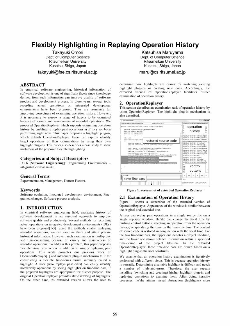
Flexibly Highlighting in Replaying Operation History Takayuki Omori

Dept. of Computer Science Ritsumeikan University Kusatsu, Shiga, Japan

[email protected]

Katsuhisa Maruyama Dept. of Computer Science

Ritsumeikan University Kusatsu, Shiga, Japan

[email protected]

ABSTRACT In empirical software engineering, historical information of software development is one of significant facets since knowledge derived from such information can improve quality of software product and development process. In these years, several tools recording actual operations on integrated development environments have been proposed. They are promising for improving correctness of examining operation history. However, it is necessary to narrow a range of targets to be examined because of variety and massiveness of recorded operations. We proposed OperationReplayer which supports examining operation history by enabling to replay past operations as if they are been performing right now. This paper proposes a highlight plug-in, which extends OperationReplayer. Users can rapidly identify target operations of their examinations by using their own highlight plug-ins. This paper also describes a case study to show usefulness of the proposed flexible highlighting.

Categories and Subject Descriptors D.2.6 [Software Engineering]: Programming Environments – integrated environments.

General Terms Experimentation, Management, Human Factors.

Keywords Software evolution, Integrated development environment, Fine-grained changes, Software process analysis.

1. INTRODUCTION In empirical software engineering field, analyzing history of software development is an essential approach to improve software quality and productivity. Several methods for recording actual operations on integrated development environments (IDEs) have been proposed[1-3]. Since the methods enable replaying recorded operations, we can examine them and attain precise historical information. However, such examination is fault-prone and time-consuming because of variety and massiveness of recorded operations. To address this problem, this paper proposes flexible visual abstraction in addition to simply replaying past operations. This work promotes our previous work of OperationReplayer[1] and introduces plug-in mechanism to it for constructing a flexible time-series visual summary called a highlight. A user (who replays past edits) can easily identify noteworthy operations by seeing highlights on time-line bars, if the prepared highlights are appropriate for his/her purpose. The original OperationReplayer provides static drawing of highlights. On the other hand, its extended version allows the user to

determine how highlights are drawn by switching existing highlight plug-ins or creating new ones. Accordingly, the extended version of OperationReplayer facilitates his/her examination of operation history.

2. OperationReplayer This section describes an examination task of operation history by using OperationReplayer. The highlight plug-in mechanism is also described.

restored+source+code

operationhistory

control+buttons

time&line+bars

Figure 1. Screenshot of extended OperationReplayer

2.1 Examination of Operation History Figure 1 shows a screenshot of the extended version of OperationReplayer. Appearance of the window is similar between the original and extended one. A user can replay past operations in a single source file on a single replayer window. He/she can change the focal time by pushing control buttons, selecting an operation from the operation history, or specifying the time on the time-line bars. The content of source code is restored in conjunction with the focal time. For the two time-line bars, the upper one denotes a project life-time, and the lower one shows detailed information within a specified time-period of the project life-time. In the extended OperationReplayer, these time-line bars are drawn based on a highlight plug-in the user constructs. We assume that an operation-history examination is iteratively performed with different views. This is because operation history is versatile. Determining a suitable highlight is difficult and needs a number of trials-and-errors. Therefore, the user repeats installing (switching and creating) his/her highlight plug-in and replaying operations to examine them. After doing iterative processes, he/she attains visual abstraction (highlights) more

59

suitable for his/her purpose. Thus, flexible highlighting is essential for the examination of the operation history.

2.2 Highlight Plug-in A highlight plug-in is implemented as an extension for highlightPoint extension point of OperationReplayer. Using APIs provided by OperationReplayer, the plug-in can access various kinds of information on recorded operations, such as the time when the operation was performed, the name of the developer who performed the operation, the deleted/inserted string, and the offset where the operation was performed. Moreover, OperationReplayer provides APIs for accessing any snapshot of source code in the past and its syntactical information. To display highlights on the time-line bars, the plug-in instantiates SpotHighlight and/or RangeHighlight. These instances are responsible for drawing lines and rectangles corresponding to times and time-periods specified on the time-line bars.

3. Case Study To show usefulness of flexible highlighting proposed here, we have created a highlight plug-in and used it to examine actual operation history. In this case study, the purpose of this examination is to distinguish periods for intensive refactoring from ones for other modifications. We checked if the created highlight plug-in has been improved in three trials. 1st trial: In the operation history, all refactoring operations invoked by Eclipse's menu items are held as instances of TriggeredOperations. The initial plug-in simply creates SpotHighlight instances corresponding to the operations, which are colored with blue (blue highlights). In addition, all operations that delete any character (the length of the deleted text is not zero) are colored with cyan (cyan highlights). The highlight plug-in has 49 lines of source code. We applied this highlight plug-in to all operations recorded in real software development. As a result, the plug-in created a large number of highlights including noises shown on the window. The noises obscured true refactorings. Figure 2(a) shows a part of the time-line bar resulting from this trial. 2nd trial: To reduce the noise, we removed the cyan highlights (a single line of source code was deleted). Instead, to detect move operations of fields and methods which are frequently done in refactorings, cut and paste operations are colored with red and orange, respectively (six lines of source code were inserted). We applied this new version of the plug-in to the same recorded operations. The result was better than one in the 1st trial; however it still includes many noises. By replaying operations around several blue highlights, we found some of the highlights involve "organize/add imports" operations that do not seem to be refactorings.

3rd trial: To further reduce noisy highlights, we improved the algorithm related to blue highlights. Finally, the plug-in detects operations of which labels are same as Eclipse's "Refactor" submenu items and colors them with blue (ten lines of source code were inserted). Applying this plug-in, we detected a possible refactoring period with intensive blue (deeply colored) lines shown in Figure 2(b). Each of these lines indicates a "rename" refactoring operation.

too+many+highlights+(in+40+min.)

(a) Highlights including many noises (1st trial)

six+refactorings (blue+highlights)

(b) Detecting intensive refactoring operations (3rd trial) Figure 2. Case study

To assess that the highlight plug-in is truly improved through this experiment, we manually examined operations around intensive highlights reported by the highlight plug-ins in 2nd and 3rd trials. Actually, we intuitively extracted several time-periods based on our understanding for the reported highlights, and then checked if each period involves true refactorings. We did not examine highlights reported in the 1st trial since it created too many worthless highlights. As a result, in the 2nd and 3rd trials, the highlight plug-in totally detected 66 and 47 refactoring periods, respectively. In both the trials, 16 true refactoring periods were detected among them. Besides, 50 and 31 faulty periods were respectively reported. The precision rates are 24% (16/66) and 34% (16/47), respectively. From these experimental results, the precision was improved with little effort (inserting and deleting source code) although the experiment is quite limited. Here, we were supposed to count the total number of periods for real refactorings within the development and show recall rates in this experiment. However, we could not precisely count it due to vast numbers of recorded operations.

4. Conclusion This paper proposed an operation replayer with a mechanism supporting flexible highlighting. It allows users to flexibly change visual abstraction of operation history on a window of OperationReplayer. We are planning to extend it to effectively treat histories of multiple source files and developers. Enhancing flexibility and scalability of visualization is also future work.

5. REFERENCES [1] Omori, T. and Maruyama, K. 2009. Identifying Stagnation

Periods in Software Evolution by Replaying Editing Operations. In Proceedings of 16th Asia-Pacific Software Engineering Conference, 389-396.

[2] Robbes, R. and Lanza, M. 2007. A Change-based Approach to Software Evolution. Electronic Notes in Theoretical Computer Science (ENTCS), 166:93-109.

[3] Hattori, L., Lungu, M., and Lanza, M. 2010. Replaying Past Changes in Multi-developer Projects. In Proceedings of IWPSE-EVOL 2010, 13-22.

60

proceedings - 情報科学研究科 | naist...

Documents