problems differential equations

Universidad San Pablo - CEU

Dynamic Systems in Biomedical Engineering

Problems

Author:

Second Year Biomedical

Engineering

Supervisor:

Carlos Oscar S. Sorzano

February 10, 2015

1 Chapter 1

Kreyszig, 1.1.2Carlos Oscar Sorzano, Aug. 31st, 2014

Solve the ODE

y′ + xe−x2

2 = 0

Solution:

y′ =dy

dx= −xe− x

2

2

By separating variables

dy = −xe− x2

2 dx

and integrating ∫dy =

∫−xe− x

2

2 dx

y = e−x2

2 + C


Solve the ODEy′ = 4e−x cos(x)

Solution:

y′ =dy

dx= 4e−x cos(x)

By separating variablesdy = 4e−x cos(x)dx

and integrating ∫dy =

∫4e−x cos(x)dx

Let's integrate by parts:

I1 =∫e−x cos(x)dx [u = e−x, dv = cos(x)dx]

= e−x sin(x)−∫

sin(x)(−e−xdx)= e−x sin(x) +

∫sin(x)e−xdx [u = e−x, dv = sin(x)dx]

= e−x sin(x) + e−x(− cos(x))−∫

(− cos(x))(−e−xdx)= e−x sin(x)− e−x cos(x)−

∫cos(x)e−xdx

= e−x sin(x)− e−x cos(x)− I1 ⇒2I1 = e−x sin(x)− e−x cos(x)⇒I1 = e−x sin(x)−cos(x)

2

Finally

y = 4I1 + C = 2(sin(x)− cos(x))e−x + C

Kreyszig, 1.1.6

1

Carlos Oscar Sorzano, Aug. 31st, 2014

Solve the ODEy′′ = −y

Solution: Let us try a particular solution of the form

y = eλx

y′ = λeλx

y′′ = λ2eλx

Then, substituting these functions in the ODE

λ2eλx = −eλx

λ2 = −1⇒ λ = ±i

So the two functionsy1 = eix

andy2 = e−ix

are solutions of the ODE. Actually, any function of the form

y = c1y1 + c2y2 = c1eix + c2e

−ix

is also a solution. In fact, it is the general solution of the ODE. Let us checkthis statement

y′ = ic1eix − ic2e−ix

y′′ = −c1eix − c2e−ix

Substituting in the ODEy′′ = −y

−c1eix − c2e−ix = −(c1eix + c2e

−ix)

As can be easily seen the function

y = c1eix + c2e

−ix + C

with C 6= 0 is not a solution of the ODE

−c1eix − c2e−ix 6= −(c1eix + c2e

−ix + C)


Solve the ODEy′ = cosh(5.13x)

Solution: To solve the proposed ODE we rewrite it as

dy

dx= cosh(5.13x)

2

Consequentlydy = cosh(5.13x)dx

Integrating ∫dy =

∫cosh(5.13x)dx

y =1

5.13sinh(5.13x) + C


Solve the ODEy′′′ = e−0.2x

Solution: Let us de�ney1 = y′

y2 = y′1 = y′′

Then the ODE can be rewritten as

y′2 = e−0.2x

whose solution isdy2 = e−0.2xdx

y2 =1

−0.2e−0.2x + c1 = −5e−0.2x + c1

Now we solve the equation

y′1 = y2 = −5e−0.2x + c1

dy1 = (−5e−0.2x + c1)dx

y1 = 25e−0.2x + c1x+ c2

And, �nally, the equation

y′ = y1 = 25e−0.2x + c1x+ c2

dy = (25e−0.2x + c1x+ c2)dx

y = −125e−0.2x +c12x2 + c2x+ c3

Since c1 is an arbitrary constant, we can absorb the 12 factor into c1, so that the

general solution is

y = −125e−0.2x + c1x2 + c2x+ c3


3

1. Verify that y = ce−2.5x2

is a solution of the ODE

y′ + 5xy = 0

2. Determine from y the particular solution of the ODE that satis�es theinitial condition y(0) = π.

3. Graph the solution of the IVP.

Solution:

1. Let us calculate y′ and substitute it into the ODE

y′ = −5cxe−2.5x2(−5cxe−2.5x2

)+ 5x

(ce−2.5x2

)= 0

−5cxe−2.5x2

+ 5cxe−2.5x2

= 00 = 0

So y is actually a solution of the ODE.

2. To satisfy the initial condition we need

y(0) = π = ce−2.5(0)2 = ce0 = c

that is, we need c = π. The particular solution ful�lling the initial condi-tion is

yp = πe−2.5x2

3. In MATLAB:

x=[-3:0.001:3]; plot(x,pi*exp(-2.5*x.�2)); xlabel('x');

−3 −2 −1 0 1 2 30

0.5

1

1.5

2

2.5

3

3.5

x


4

1. Verify that y2 − 4x2 = C is a solution of the ODE

yy′ = 4x

2. Determine from y the particular solution of the ODE that satis�es theinitial condition y(1) = 4.

3. Graph the solution of the IVP.

Solution:

1. Let us di�erentiate the equation de�ning the implicit function

Dx(y2 − 4x2 = C)2yy′ − 8x = 0yy′ = 4x

that is exactly the ODE, so the implicit function de�ned by y2− 4x2 = Cis actually a solution of the proposed ODE.

2. To satisfy the initial condition y(1) = 4 we need

y2 − 4x2 = C

(4)2 − 4(1)2 = C

C = 16− 4 = 12

So the particular solution satisfying the given initial condition is

y2p − 4x2 = 12

3. In MATLAB:

h=ezplot('y.�2-4*x.�2-12',[-3 3 -10 10]);

set(h,'Color','b')

x

y

y2−4 x2−12 = 0

−3 −2 −1 0 1 2 3−10

−8

−6

−4

−2

0

2

4

6

8

10

5


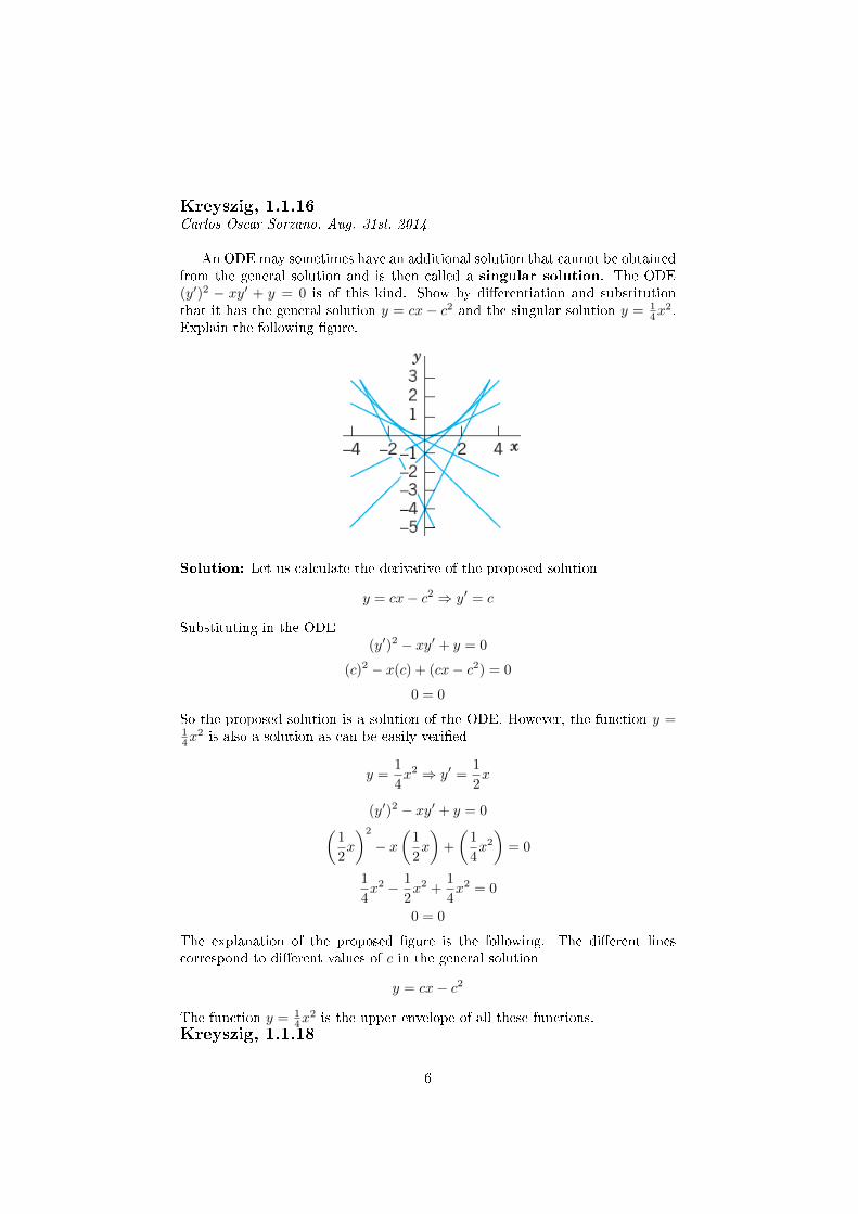
An ODE may sometimes have an additional solution that cannot be obtainedfrom the general solution and is then called a singular solution. The ODE(y′)2 − xy′ + y = 0 is of this kind. Show by di�erentiation and substitutionthat it has the general solution y = cx− c2 and the singular solution y = 1

4x2.

Explain the following �gure.

Solution: Let us calculate the derivative of the proposed solution

y = cx− c2 ⇒ y′ = c

Substituting in the ODE(y′)2 − xy′ + y = 0

(c)2 − x(c) + (cx− c2) = 0

0 = 0

So the proposed solution is a solution of the ODE. However, the function y =14x

2 is also a solution as can be easily veri�ed

y =1

4x2 ⇒ y′ =

1

2x

(y′)2 − xy′ + y = 0(1

2x

)2

− x(

1

2x

)+

(1

4x2

)= 0

1

4x2 − 1

2x2 +

1

4x2 = 0

0 = 0

The explanation of the proposed �gure is the following. The di�erent linescorrespond to di�erent values of c in the general solution

y = cx− c2

The function y = 14x

2 is the upper envelope of all these functions.Kreyszig, 1.1.18

6


Radium 22888 Ra has a half-life of about 3.6 days.

1. Given 1 gram, how much will still be present after 1 day?

2. After 1 year?

Solution: Radioactive desintegration responds to the linear ODE

dA

dt= −Kt

whose general solution is

A(t) = A(0)e−Kt t > 0

Note that the units of K are [time−1]. We can also write the general solutionas

A(t) = A(0)e−tτ t > 0

where the units of τ are now [time].A half-life of 3.6 days implies that

A(3.6) =A(0)

2= A(0)e−

3.6τ

− log(2) = −3.6

τ

τ =3.6

log(2)= 5.1937[days]

At this point we can answer the two questions:

1. After 1 day there is: A(1) = A(0)e−1τ = 1e−

15.1937 = 0.8249[g].

2. After 1 year there is: A(365) = A(0)e−365τ = 1e−

3655.1937 = 3 · 10−31[g].


In dropping a stone or an iron ball, air resistance is practically negligible.Experiments show that the acceleration of the motion is constant (equal tog = 9.80[m/s2], called the acceleration of gravity). Model this as an ODE fory(t), the distance fallen as a function of time t. If the motion starts at timet = 0 from rest (i.e., with velocity v = y′ = 0), show that you obtain the familiarlaw of free fall

y =1

2gt2

Solution: Let us understand the physical meaning of each of the variablesinvolved:

• y(t) is the distance fallen at time t

• y′(t) is the speed of the object at time t

7

• y′′(t) is its acceleration at time t

The fact that acceleration is constant along the fall implies

y′′ = g

Let us de�ne the variablev = y′

Then, the free fall ODE can be written as

v′ = g

dv = gdt

v = gt+ c

But the object is at rest at t = 0, that is

v(0) = 0 = g(0) + c⇒ c = 0

Now we solve the equationv = y′

for ydy = vdt = gtdt

y =1

2gt2 + c

At time t = 0 the object had not moved, that is

y(0) = 0 =1

2g(0)2 + c⇒ c = 0

Finally, the solution of the falling ODE is

y =1

2gt2


Graph a direction �eld (by a CAS or by hand) for the ODE

y′ = 2y − y2

In the �eld graph several solution curves by hand, particularly those passingthrough the points (0, 0), (0, 1), (0, 2), (0, 3).Solution: In MATLAB

[x,y]=meshgrid(-1:0.25:5,-2:0.25:4);

f = @(x,y) 2*y-y.�2;

dy=feval(f,x,y);

dx=ones(size(dy));

quiver(x,y,dx,dy);

axis([-1 5 -2 4])

8

xlabel('x')

ylabel('y')

hold on

% (0,0)

[xa,ya] = ode45(f,[0,5],0);

[xb,yb] = ode45(f,[0,-1],0);

plot(xa,ya,'b','LineWidth',2)

plot(xb,yb,'b','LineWidth',2)

% (0,1)

[xa,ya] = ode45(f,[0,5],1);

[xb,yb] = ode45(f,[0,-1],1);

plot(xa,ya,'r','LineWidth',2)

plot(xb,yb,'r','LineWidth',2)

% (0,2)

[xa,ya] = ode45(f,[0,5],2);

[xb,yb] = ode45(f,[0,-1],2);

plot(xa,ya,'k','LineWidth',2)

plot(xb,yb,'k','LineWidth',2)

% (0,3)

[xa,ya] = ode45(f,[0,5],3);

[xb,yb] = ode45(f,[0,-1],3);

plot(xa,ya,'g','LineWidth',2)

plot(xb,yb,'g','LineWidth',2)

−1 0 1 2 3 4 5−2

−1

0

1

2

3

4

x

y


9

Graph a direction �eld (by a CAS or by hand) for the ODE

y′ = x− 1

y

In the �eld graph several solution curves by hand, particularly that one passingthrough the point (1, 1

2 ).Solution: In MATLAB

[x,y]=meshgrid(-2:0.15:2,0.15:0.15:2);

f = @(x,y) x-1./y;

dy=feval(f,x,y);

dx=ones(size(dy));

quiver(x,y,dx,dy);

axis([-2 2 0.15 2])

xlabel('x')

ylabel('y')

hold on

% (1,0.5) [xa,ya] = ode45(f,[1,1.2],0.5);

[xb,yb] = ode45(f,[1,-2],0.5);

plot(xa,ya,'r','LineWidth',2)

plot(xb,yb,'r','LineWidth',2)

−2 −1.5 −1 −0.5 0 0.5 1 1.5 2

0.2

0.4

0.6

0.8

1

1.2

1.4

1.6

1.8

2

x

y


An ODE is autonomous if it does not show x (the independent variable)explicitly in f

y′ = f(x, y)

For instance,y′ = sin2(y)

10

y′ = −5y12

What will the level curves f(x, y) = const (also called isoclines, of equal incli-nation) of an autonomous ODE look like? Give reason.Solution: They are lines parallel to the x axis, since all points with the same xhave the same inclination (slope of the tangent). For example, for the equation

y′ = sin2(y)

we would have in MATLAB

[x,y]=meshgrid(-pi:0.25:pi,-pi:0.25:pi);

f = @(x,y) (sin(y)).�2;

dy=feval(f,x,y);

dx=ones(size(dy));

quiver(x,y,dx,dy);

axis([-pi pi -pi pi])

xlabel('x')

ylabel('y')

hold on

% Isoclines

contour(x,y,dy./dx,0.25,'r','LineWidth',2)

contour(x,y,dy./dx,0.75,'g','LineWidth',2)

−3 −2 −1 0 1 2 3−3

−2

−1

0

1

2

3

x

y


Two forces act on a parachutist, the attraction by the earth mg (m is themass of person plus equipment, g = 9.8[m/s2] the acceleration of gravity) andthe air resistance, assumed to be proportional to the square of the velocity v(t).Using Newton's second law of motion (mass × acceleration = resultant of the

11

forces), set up a model (an ODE for v(t)). Graph a direction �eld (choosingm and the constant of proportionality equal to 1). Assume that the parachuteopens when v = 10[m/s]. Graph the corresponding solution in the �eld. What isthe limiting velocity? Would the parachute still be su�cient if the air resistancewere only proportional to v(t)?Solution: The following equation for the velocity v re�ects the physical knowl-edge of the problem

mv′ = mg − νv2

With m = 1[kg] and ν = 1[Ns2/kg], we have

v′ = g − v2

If the parachute opens at v = 10[m/s] it means

v(0) = 10

we would have in MATLAB (see red curve)

[x,v]=meshgrid(0:0.1:2,0:0.5:10);

f = @(x,v) 9.8-v.�2;

dv=feval(f,x,v);

dx=ones(size(dv));

quiver(x,v,dx,dv);

axis([0 2 0 10])

xlabel('t')

ylabel('v')

hold on

% Solution

[t10,v10]=ode45(f,[0 2],10);

plot(t10,v10,'r','LineWidth',2)

If the air resistance were proportional to v(t), then (see black curve)

v′ = g − v

It can be seen that the decrease of speed is much slower:

12

0 0.5 1 1.5 2

3

4

5

6

7

8

9

10

t

v

Kreyszig, 1.2.17Álvaro Martín Ramos, Dec. 25th, 2014

Apply Euler's method to the ODE

y′ = y

with h = 0.1 and y(0) = 1.Solution: The method applied to this case would give

y0 = y(0) = 1y1 = y0 + hf(x0, y0) = 1 + 0.1(y0) = 1 + 0.1(1) = 1.1y2 = y1 + hf(x1, y1) = 1.1 + 0.1(y1) = 1.1 + 0.1(1.1) = 1.21y3 = y2 + hf(x2, y2) = 1.11 + 0.1(y2) = 1.21 + 0.1(1.21) = 1.331...


Apply Euler's method to the ODE

y′ = −5x4y2 y(0) = 1

with h = 0.2. The true solution is

y =1

(1 + x)5

Solution: The method applied to this case would give

y0 = y(0) = 1y1 = y0 + hf(x0, y0) = 1 + 0.2(−5x4

0y20) = 1 + 0.2(−5(0)4(1)2) = 1

y2 = y1 + hf(x1, y1) = 1 + 0.2(−5x41y

21) = 1 + 0.2(−5(0.2)4(1)2) = 0.9984

y3 = 0.9729y4 = 0.8502...

13

In MATLAB

f = @(x,y) -5*x.�4.*y.�2;

% Euler

y=zeros(10,1);

x=zeros(10,1);

x(1)=0; y(1)=1; % y(0)=1

h=0.2;

for k=1:length(y)-1

y(k+1)=y(k)+h*f(x(k),y(k));

x(k+1)=x(k)+h;

end

% ODE45

[xRK,yRK]=ode45(f,[0,1.8],1);

% True solution

xt=0:0.01:1.8;

yt=1./((xt+1).�5);

plot(x,y,xRK,yRK,xt,yt)

legend('Euler solution','Runge-Kutta 45','True solution')

xlabel('x')

ylabel('y')

0 0.2 0.4 0.6 0.8 1 1.2 1.4 1.6 1.80

0.1

0.2

0.3

0.4

0.5

0.6

0.7

0.8

0.9

1

x

y

Euler solution h=0.2Runge−Kutta 45True solution


Solvey3 + y′ + x3 = 0

14

Solution: We can rearrange the equation as

y′ = −x3

y3= −

(x

y

)3

We see that the equation has the form

y′ = f(yx

)so that it can be reduced to a separable form by making the change of variables

u =y

x⇒ y = xu⇒ y′ = u′x+ u

Substituting in the ODE

u′x+ u = − 1

u3

u′x = −(u+

1

u3

)= −u

4 + 1

u3

Separating variablesu3

u4 + 1du = − 1

xdx

Integrating ∫u3

u4 + 1du = −

∫1

xdx

1

4

∫4u3

u4 + 1du = − log |x|+ C

Solving for u1

4log |u4 + 1| = − log |x|+ C

log |u4 + 1| 14 = − log |x|+ C

|u4 + 1| 14 =C

x

u4 + 1 =C

x4

And undoing the change of variable(yx

)4

+ 1 =C

x4

y4 + x4 = C

Kreyszig, 1.3.7Carlos Oscar Sorzano, Nov. 2nd, 2014

Solvexy′ = y + 2x3 sin2

(yx

)

15

by making the change of variables yx = u

Solution: The change of variables yx = u implies

y = ux

y′ = u′x+ u

Substituting in the di�erential equation we get

x(u′x+ u) = ux+ 2x3 sin2(u)

x2u′ = 2x3 sin2(u)

u′

sin2(u)= 2x

du

sin2(u)= 2xdx

Integrating we get

− 1

tan(u)= x2 + C

tan(u) =1

C − x2

u = arctan1

C − x2

Undoing the change of variable

y = ux = x arctan1

C − x2


Solvey′ = (y + 4x)2

by making the change of variables y + 4x = vSolution:

y + 4x = v ⇒ y′ + 4 = v′ ⇒ y′ = v′ − 4

Substituting in the ODEv′ − 4 = v2

v′ = v2 + 4

v′

v2 + 4= 1

Separating variablesdv

v2 + 4= dx

Integrating ∫dv

v2 + 4=

∫dx

16

∫1

4

dv

( v2 )2 + 1= x+ C

1

2

∫ 12dv

( v2 )2 + 1= x+ C

1

2atan

v

2= x+ C

Solving for vv = 2 tan(2x+ C)

Undoing the change of variables

y + 4x = 2 tan(2x+ C)

y = −4x+ 2 tan(2x+ C)


If the growth rate of the number of bacteria at any time t is proportionalto the number present at t and doubles in 1 week, how many bacteria can beexpected after 2 weeks? After 4 weeks?Solution: The growth rate of the number of bacteria is A′(t). If it is propor-tional to the number of bacteria, we have

A′ = µA

whose solution can be obtained by separating variables

dA = µAdt

dA

A= µdt

Integratinglog |A| = µt+ C

Solving for AA = Ceµt

If the number of bacteria doubles every week, we have

A(t+ 7) = 2A(t)

Ceµ(t+7) = 2Ceµt

eµ7 = 2⇒ µ =log(2)

7= 0.0990

After 2 weeks we will have

A(t+ 14) = Ceµ(t+14) = Ceµteµ14 = A(t)elog(2)

7 14 = A(t)e2 log(2) = A(t)(elog(2))2 = A(t)22 = 4A(t)

Similarly, after 4 weeks, we will have

A(t+ 28) = A(t)elog(2)

7 28 = A(t)e4 log(2) = A(t)(elog(2))4 = A(t)24 = 16A(t)

17


1. If the birth rate and death rate of the number of bacteria are proportionalto the number of bacteria present, what is the population as a function oftime.

2. What is the limiting situation for increasing time? Interpret it.

Solution:

1. The following model describes the situation

A′ = µbA− µdA = (µb − µd)A

Similarly to Problem 1.3.19, its solution is

A = Ce(µb−µd)t = A(0)e(µb−µd)t

2. If µb = µd, the number of bacteria stays stable from t = 0. If µb > µd,the number of bacteria grows exponentially. On the contrary, if µb < µd,the number of bacteria exponentially decreases to 0.


Boyle�Mariotte's law for ideal gases. Experiments show for a gas atlow pressure P (and constant temperature) the rate of change of the volumeV (P ) equals −VP . Solve the model.Solution: The following ODE models the system

V ′ = −VP

V ′

V= − 1

P

Separating variablesdV

V= −dP

P

Integrating

log |V | = − log |P |+ C = log

∣∣∣∣CP∣∣∣∣

V =C

P


18

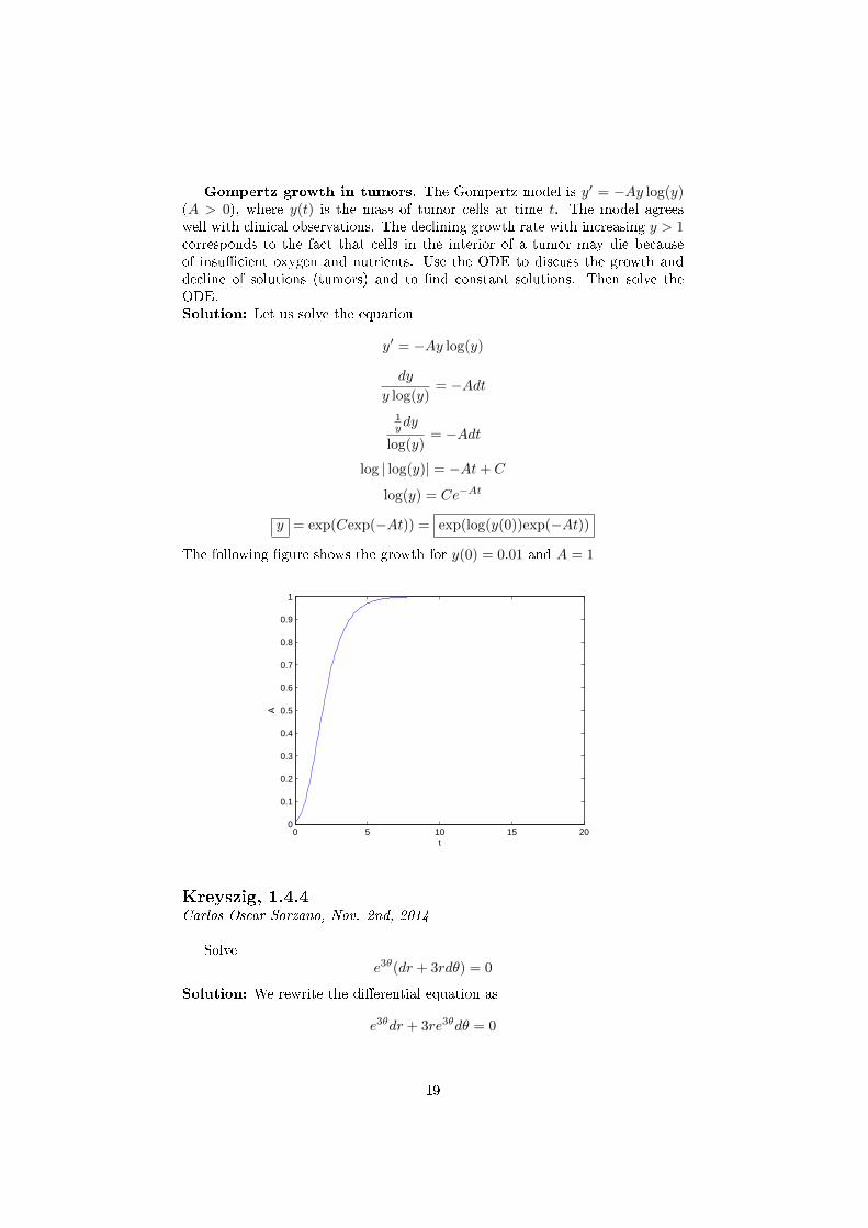
Gompertz growth in tumors. The Gompertz model is y′ = −Ay log(y)(A > 0), where y(t) is the mass of tumor cells at time t. The model agreeswell with clinical observations. The declining growth rate with increasing y > 1corresponds to the fact that cells in the interior of a tumor may die becauseof insu�cient oxygen and nutrients. Use the ODE to discuss the growth anddecline of solutions (tumors) and to �nd constant solutions. Then solve theODE.Solution: Let us solve the equation

y′ = −Ay log(y)

dy

y log(y)= −Adt

1ydy

log(y)= −Adt

log | log(y)| = −At+ C

log(y) = Ce−At

y = exp(Cexp(−At)) = exp(log(y(0))exp(−At))

The following �gure shows the growth for y(0) = 0.01 and A = 1

0 5 10 15 200

0.1

0.2

0.3

0.4

0.5

0.6

0.7

0.8

0.9

1

t

A


Solvee3θ(dr + 3rdθ) = 0

Solution: We rewrite the di�erential equation as

e3θdr + 3re3θdθ = 0

19

which is of the formPdr +Qdθ = 0

To check if it is an exact equation we calculate

∂P

∂θ= 3e3θ

∂Q

∂r= 3e3θ

Since both partial derivatives are equal, the equation is exact and we look for asolution of the form

U =

∫Pdr + C(θ) =

∫e3θdr + C(θ) = e3θr + C(θ)

To determine the constant C(θ) we di�erentiate this function with respect to θ

∂U

∂θ= 3re3θ + C ′(θ)

and compare it to Q3re3θ + C ′(θ) = Q

3re3θ + C ′(θ) = 3re3θ

C ′(θ) = 0

Integrating with respect to θC(θ) = C

Finally, the implicit solution of the di�erential equation is

e3θr + C = 0

or explicitlyr = −Ce−3θ


Solve the ODEex(cos(y)dx− sin(y)dy) = 0

Solution: We may rewrite the ODE as

ex cos(y)dx− ex sin(y)dy = 0

That is of the formP (x, y)dx+Q(x, y)dy = 0

To see if it is exact we calculate

∂P

∂y= ex(− sin(y))

20

∂Q

∂x= −ex sin(y)

Since ∂P∂y = ∂Q

∂x , the ODE is exact. To �nd the solution, u that satis�es

∂u

∂x= P

∂u

∂y= Q

we integrate P with respect to x

u(x, y) =∫ex cos(y)dx = cos(y)ex + C(y)

If we now di�erentiate u with respect to y we should obtain Q

∂u

∂y= ex(− sin(x)) + C ′(y) = −ex sin(y)⇒ C ′(y) = 0⇒ C(y) = C

So the solution to the problem are all functions of the form

u(x, y) = C = cos(y)ex ⇒ y = acos(Ce−x)


Solve the ODEe2x(2 cos(y)dx− sin(y)dy) = 0


e2x2 cos(y)dx− e2x sin(y)dy) = 0



∂P

∂y= −2e2x sin(y)

∂Q

∂x= −2e2x sin(y)

Since∂Q

∂x=∂P

∂y

the ODE is exact. To �nd the solution, u, that satis�es

∂u

∂x= P

∂u

∂y= Q

we integrate P with respect to x

u(x, y) =

∫e2x2 cos(y)dx = cos(y)e2x + C(y)

21

If we now di�erentiate u with respect to y we should obtain Q

∂u

∂y= − sin(y)e2x + C ′(y) = −e2x sin(y)⇒ C ′(y) = 0⇒ C(y) = C

So the solution to the problem are all functions of the form

u(x, y) = C = cos(y)e2x ⇒ y = acos(Ce−2x)

Kreyszig, 1.4.10Carlos Oscar Sorzano, Jan. 13th, 2015

Solve the di�erential equation

ydx+ (y + tan(x+ y))dy = 0

knowing that cos(x+ y) is an integrating factor.Solution: Let us multiply the whole equation by cos(x+ y)

y cos(x+ y)dx+ (y cos(x+ y) + sin(x+ y))dy = 0

which is of the formP (x, y)dx+Q(x, y)dy = 0

Let us check if this is an exact equation:

Py =∂P (x, y)

∂y= cos(x+ y)− y sin(x+ y)

Qx =∂Q(x, y)

∂x= −y sin(x+ y) + cos(x+ y)

Since Py = Qx, the equation is exact. We can solve it by integrating withrespect to one of the variables

U(x, y) =

∫P (x, y)dx =

∫y cos(x+ y)dx = y sin(x+ y) + C(y)

We now di�erentiate U with respect to y

Q(x, y) =∂U(x, y)

∂y

y cos(x+ y) + sin(x+ y) = sin(x+ y) + y cos(x+ y) + C ′(y)

C ′(y) = 0

C(y) = C

Finally, the implicit solution of the di�erential equation is

U(x, y) = 0

y sin(x+ y) + C = 0

22


Solve the ODE

2 cosh(x) cos(y)dx = sinh(x) sin(y)dy


2 cosh(x) cos(y)dx− sinh(x) sin(y)dy = 0



∂P

∂y= 2 cosh(x)(− sin(y))

∂Q

∂x= − cosh(x) sin(y)

Since ∂P∂y 6=

∂Q∂x , the ODE is not exact. For �nding an integrating factor, we

start by calculating

Py −Qx = 2 cosh(x)(− sin(y))− (− cosh(x) sin(y)) = − cosh(x) sin(y)

We note thatQx − Py

P=

cosh(x) sin(y)

2 cosh(x) cos(y)=

1

2tan(y)

is a function of y, f(y). The integrating factor comes

F = exp

(∫1

2tan(y)dy

)= exp

(−1

2log(cos(y))

)=

1√cos(y)

We now multiply the ODE by the integrating factor

1√cos(y)

(2 cosh(x) cos(y)dx− sinh(x) sin(y)dy) = 0

2 cosh(x)√

cos(y)dx− sinh(x)sin(y)√cos(y)

dy = 0

At this point, the ODE is exact. We �nd its solution by integrating P withrespect to x

u(x, y) =

∫2 cosh(x)

√cos(y)dx = 2 sinh(x)

√cos(y) + C(y)

Di�erentiating with respect to y we should obtain FQ

∂u

∂y= − sinh(x)

sin(y)√cos(y)

+ C ′(y) = − sinh(x)sin(y)√cos(y)

⇒ C ′(y) = 0

23

So the solutions of the ODE are of the form

u(x, y) = C = 2 sinh(x)√

cos(y)


Solve the ODExy′ = 2y + x3ex


y′ − 2

xy = x2ex

That is of the formy′ + p(x)y = r(x)

This is a linear, non-homogeneous equation, whose solution is given by

yh = e−h(

∫ehrdx+ C)

whereh =

∫pdx = −

∫2xdx = −2 log |x|

e−h = e2 log |x| = x2∫ehrdx =

∫(x−2)(x2ex)dx = ex

Finally

y = x2(ex + C)


Solve the ODEy′ = 6(y − 2.5)tanh(1.5x)


y′ − 6tanh(1.5x)y = −15tanh(1.5x)

That is of the formy′ + p(x)y = r(x)

This is a linear, non-homogeneous equation, whose solution is given by

yh = e−h(

∫ehrdx+ C)

where

h =∫pdx = −6

∫tanh(1.5x)dx = −6 log(cosh(1.5x))

1.5 = −4 log(cosh(1.5x))

e−h = e4 log(cosh(1.5x)) = cosh4(1.5x)∫ehrdx =

∫(cosh−4(1.5x))(−15tanh(1.5x))dx = 2.5

cosh4(1.5x)

24

Finally

y = cosh4(1.5x)

(2.5

cosh4(1.5x)+ C

)= 2.5 + C cosh4(1.5x)


Let H be the homogeneous problem

y′ + p(x)y = 0

and NH be the non-homogeneous problem

y′ + p(x)y = r(x)

Show that the sum of two solutions and of the homogeneous equation (H) is asolution of (H), and so is a scalar multiple for any constant a. These propertiesare not true for the non-homogeneous problem (NH).Solution: Let y1 and y2 be two solutions of the homogeneous problem so that

y′1 + p(x)y1 = 0

y′2 + p(x)y2 = 0

Adding both equations we have

y′1 + y′2 + p(x)y1 + p(x)y2 = 0

(y1 + y2)′ + p(x)(y1 + y2) = 0

This last equation proves that y1 + y2 is also a solution of the homogeneousproblem. Similarly if we multiply the �rst equation by a we have

a(y′1 + p(x)y1) = 0

ay′1 + ap(x)y1 = 0

(ay1)′ + p(x)(ay1) = 0

which proves that ay1 is also a solution of the homogeneous problem.However, this is not true for the non-homogeneous problem. Let us assume

that y1 and y2 are solutions of the non-homogeneous problem

y′1 + p(x)y1 = r(x)

y′2 + p(x)y2 = r(x)

Let us check if y1 + y2 is also a solution. For doing so, we substitute y1 + y2

into the ODE

(y1 + y2)′ + p(x)(y1 + y2) = (y′1 + p(x)y1) + (y′2 + p(x)y2) = 2r(x) 6= r(x)

The same happens with ay1

(ay1)′ + p(x)(ay1) = a(y′1 + p(x)y1) = ar(x) 6= r(x)

25


Show that the sum of a solution of the non-homogeneous problem and asolution of the homogeneous one is a solution of the non-homogeneous problem.Solution: Let yp be a solution of the non-homogeneous problem

y′p + p(x)yp = r(x)

and yh be a solution of the homogeneous problem

y′h + p(x)yh = 0

Let us check if yp + yh is a solution of the non-homogeneous problem

(yp + yh)′ + p(x)(yp + yh) = (y′p + p(x)yp) + (y′h + p(x)yh) = r(x) + 0 = r(x)

That is, yp + yh is indeed a solution of the non-homogeneous problem.Kreyszig, 1.5.18Carlos Oscar Sorzano, Aug. 31st, 2014

Show that the di�erence of two solutions of the non-homogeneous problemis a solution of the homogeneous problem.Solution: Let yp1 and yp2 be two solutions of the non-homogeneous problem

y′p1 + p(x)yp1 = r(x)

y′p2 + p(x)yp2 = r(x)

Let us check if yp1 − yp2 is a solution of the homogeneous problem

(yp1−yp2)′+p(x)(yp1−yp2) = (y′p1 +p(x)yp1)−(y′p2 +p(x)yp2) = r(x)−r(x) = 0

That is, yp1 − yp2 is indeed a solution of the homogeneous problem.Kreyszig, 1.5.21Carlos Oscar Sorzano, Aug. 31st, 2014

Variation of parameter. Another method of obtaining the solution y =e−h(

∫ehrdx+ C) of a non-homogeneous problem

y′ + p(x)y = r(x)

results from the following idea. Write the solution of the homogeneous problemas

y = Ce−∫pdx = Ce−h = Cy∗

where y∗ is the exponential function, which is a solution of the homogeneouslinear ODE

(y∗)′ + p(x)y∗ = 0

Replace the arbitrary constant C in the homogeneous solution with a functionu to be determined so that the resulting function y = uy∗ is a solution of thenonhomogeneous linear ODE.

26

Solution: Let us introduce the function uy∗ into the non-homogeneous ODEto see the requirements that u must meet

(uy∗)′ + p(uy∗) = u′y∗ + u(y∗)′ + puy∗

= u′y∗ + u((y∗)′ + py∗)= u′y∗ + u0= u′y∗

= r

That is, we need

u′y∗ = r ⇒ u′ = re−h

= reh ⇒ u =∫rehdx+ C

So the solution of the non-homogeneous problem is

y = uy∗ =

(∫rehdx+ C

)e−h


Solve y′ + y = −xySolution: This is a Bernouilli equation of the form

y′ + p(x)y = g(x)ya

with p(x) = 1, g(x) = −x and a = −1. We do the change of variable

u = y1−a = y1−(−1) = y2

Di�erentiating

u′ = 2yy′ = 2y(−y − xy−1) = −2y2 − 2x = −2u− 2x

u′ + 2u = −2x

This is now a linear, non-homogeneous equation system of the form

u′ + pu = r

whose solution is given by

h =

∫pdx =

∫2dx = 2x

u = e−h(∫ehrdx+ C) = e−2x

(∫e2x(−2x)dx+ C

)= e−2x

(xe2x − 1

2e2x + C

)= x− 1

2 + Ce2x

Now we undo the change of variable

y2 =

√x− 1

2+ Ce2x

27


Solvey′ = 3.2y − 10y2


y′ − 3.2y = −10y2

This is a Bernouilli equation of the form


with p(x) = −3.2, g(x) = −10 and a = 2. We do the change of variable

u = y1−a = y1−2 = y−1

Di�erentiating

u′ = (y−1)′ = − 1

y2y′ = − 1

y2(3.2y − 10y2) = −3.2y−1 + 10 = −3.2u+ 10

u′ + 3.2u = 10


u′ + pu = r


h =

∫pdx =

∫(−3.2)dx = −3.2x

u = e−h(∫ehrdx+ C) = e3.2x(

∫e−3.2x10dx+ C)

= e3.2x( 10e−3.2x

−3.2 + C) = − 103.2 + Ce3.2x


y =1

u=

1

− 103.2 + Ce3.2x


Solve 2xyy′ + (x− 1)y2 = x2ex. Hint: set z = y2

Solution: If we do the change of variable

z = y2 ⇒ z′ = 2yy′

then the ODE is transformed to

xz′ + (x− 1)z = x2ex

28

z′ +x− 1

xz = xex


z′ + pz = r


h =

∫pdx =

∫x− 1

xdx = x− log |x|

z = e−h(∫ehrdx+ C) = e−x+log |x| (∫ ex−log |x|(xex)dx+ C

)= e−xx

(∫e2xdx+ C

)= e−xx

(12e

2x + C)

= x2 ex + Ce−x


y2 =

√x

2ex + Ce−x


Find and solve the model for drug injection into the bloodstream if, begin-ning at t = 0 a constant amount A[g/min] is injected and the drug is simul-taneously removed at a rate proportional to the amount of the drug present attime t.Solution: The ODE

A′ = Kin −KoutA A(0) = 0

models the system. This can be rewritten as

A′ +KoutA = Kin

which is a linear, non-homogeneous ODE whose solution is

h =∫Koutdt = Koutt

A = e−h(∫ehrdt+ C

)= e−Koutx

(∫eKouttKindt+ C

)= e−Koutt

(Kin

1Kout

eKoutt+ C)

= KinKout

+ Ce−Koutt

Now we impose the initial condition

A(0) = 0 =Kin

Kout+ C ⇒ C = − Kin

Kout

Finally, the solution is

A(t) =Kin

Kout(1− e−Koutt) (t > 0)

Kreyszig, 1.5.34

29


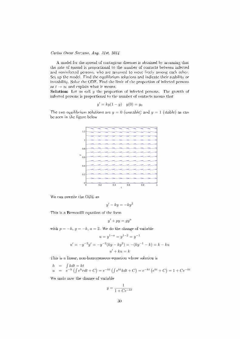
A model for the spread of contagious diseases is obtained by assuming thatthe rate of spread is proportional to the number of contacts between infectedand noninfected persons, who are assumed to move freely among each other.Set up the model. Find the equilibrium solutions and indicate their stability orinstability. Solve the ODE. Find the limit of the proportion of infected personsas t→∞ and explain what it means.Solution: Let us call y the proportion of infected persons. The growth ofinfected persons is proportional to the number of contacts means that

y′ = ky(1− y) y(0) = y0

The two equilibrium solutions are y = 0 (unstable) and y = 1 (stable) as canbe seen in the �gure below

0 0.2 0.4 0.6 0.8 10

0.2

0.4

0.6

0.8

1

1.2

t

y

We can rewrite the ODE as

y′ − ky = −ky2

This is a Bernouilli equation of the form

y′ + py = gya

with p = −k, g = −k, a = 2. We do the change of variable

u = y1−a = y1−2 = y−1

u′ = −y−2y′ = −y−2(ky − ky2) = −(ky−1 − k) = k − kuu′ + ku = k

This is a linear, non-homogeneous equation whose solution is

h =∫kdt = kt

u = e−h(∫ehrdt+ C

)= e−kt

(∫ektkdt+ C

)= e−kt

(ekt + C

)= 1 + Ce−kt

We undo now the change of variable

y =1

1 + Ce−kt

30

Imposing the initial condition

y0 =1

1 + C⇒ C =

1

y0− 1 =

1− y0

y0

Finally

y =1

1 + 1−y0y0

e−kt=

y0

y0 + (1− y0)e−kt

The following �gure shows the curve for y0 = 0.1, k = 0.8.

0 2 4 6 8 100

0.1

0.2

0.3

0.4

0.5

0.6

0.7

0.8

0.9

1

t

y


Which is the set of orthogonal trajectories to the curve family

y = ce−x2

Solution: To �nd the orthogonal trajectories, we di�erentiate the set of curves

y′ = −2xce−x2

That we may rewrite asy′ = −2xy = f(x, y)

The set of orthogonal curves must ful�ll

y′ = − 1

f(x, y)=

1

−2xy

yy′ = − 1

2x

ydy = − 1

2xdx

Which is a separable di�erential equation that can be directly integrated

1

2y2 = −1

2log(x) + C

31

y2 = − log(x) + C

ey2

=C

x

Finally, the curve family can be rewritten as

x = Ce−y2


Electric �eld. The lines of electric force of two opposite charges of thesame strength at (−1, 0) and (1, 0) are the circles through (−1, 0) and (1, 0).Show that these circles are given by

x2 + (y − c)2 = 1 + c2.

Show that the equipotential lines (which are orthogonal trajectories of thosecircles) are the circles given by

(x+ c∗)2 + y2 = (c∗)2 − 1

(dashed in the following �gure).

Solution: The curvex2 + (y − c)2 = 1 + c2

is the family of all circles pasing by (−1, 0) and (1, 0). To show this statementwe show that (−1, 0) and (1, 0) ful�ll this equation

(−1)2 + (0− c)2 = 1 + c2

(1)2 + (0− c)2 = 1 + c2

Obviously this family is a set of circles.To �nd the orthogonal trajectories, we di�erentiate the curve

2x+ 2(y − c)y′ = 0

x+ (y − c)y′ = 0

32

This curve contains the parameter c which should not be there. To eliminateit, we manipulate the original set of curves to get

x2 + y2 + c2 − 2yc = 1 + c2

x2 + y2 − 2yc = 1

c =x2 + y2 − 1

2y

So the di�erential equation becomes

x+

(y − x2 + y2 − 1

2y

)y′ = 0

2yx+(2y2 − (x2 + y2 − 1)

)y′ = 0

2yx+(y2 − x2 + 1

)y′ = 0

y′ = − 2yx

y2 − x2 + 1= f(x, y)

The set of orthogonal curves must ful�ll

y′ = − 1

f(x, y)=y2 − x2 + 1

2yx=

1

2xy +

1

2

1− x2

xy−1

y′ − 1

2xy =

1

2

1− x2

xy−1

This ODE is a Bernouilli equation of the form


with a = −1. So we make the change of variable

u = y1−a = y1−(−1) = y2 ⇒ u′ = 2yy′

u′ = 2y

(1

2xy +

1

2

1− x2

xy−1

)u′ =

1

xy2 +

1− x2

x

u′ =1

xu+

1− x2

x

u′ − 1

xu =

1− x2

x

This is a linear equation whose solution is

h =∫− 1xdx = − log |x|

eh = e− log |x| = 1x

u = e−h(∫ehrdx+ c∗

)= x

(∫1x

1−x2

x dx+ c∗)

= x(−x

2+1x + c∗

)= −x2 − 1 + c∗x

33


y2 = −x2 − 1 + c∗x

y2 + x2 − c∗x = −1

y2 + x2 − c∗x+

(c∗

2

)2

= −1 +

(c∗

2

)2

y2 +

(x− c∗

2

)2

= −1 +

(c∗

2

)2

y2 + (x− c∗)2= −1 + (c∗)2

(x+ c∗)2

+ y2 = (c∗)2 − 1


Temperature �eld. Let the isotherms (curves of constant temperature) ina body in the upper half-plane y > 0 be given by

4x2 + 9y2 = c.

. Find the orthogonal trajectories (the curves along which heat will �ow inregions �lled with heat-conducting material and free of heat sources or heatsinks).Solution: Let us analyze �rst the curves

4x2 + 9y2 = c

4

cx2 +

9

cy2 = 1(

x√c

2

)2

+

(y√c

3

)2

= 1

So they are ellipses of semiaxes√c

2 and√c

3 .Their orthogonal trajectories can be determined by di�erentiating the family

of curves:8x+ 18yy′ = 0

4x+ 9yy′ = 0

y′ = −4x

9y= f(x, y)

The orthogonal trajectories ful�ll the di�erential equation

y′ = − 1

f(x, y)=

9y

4x

dy

9y=dx

4x

34

1

9log |y| = 1

4log |x|+K

log |y| = 9

4log |x|+K

y = Kx94 = Kx2.25

In MATLAB:

close all

h=ezplot('y-x�2.25',[-2 2 0 4])

set(h,'Color','red')

hold on

h=ezplot('y-2*x�2.25',[-2 2 0 4])


h=ezplot('y-0.5*x�2.25',[-2 2 0 4])


h=ezplot('4*x�2+9*y�2=1',[-2 2 0 4])

set(h,'Color','blue')

h=ezplot('4*x�2+9*y�2=8',[-2 2 0 4])


h=ezplot('4*x�2+9*y�2=20',[-2 2 0 4])


axis square

title �

x

y

−2 −1 0 1 20

0.5

1

1.5

2

2.5

3

3.5

4

ProblemaCarlos Oscar Sorzano, Nov. 4th, 2014

It starts snowing in the morning and continues steadily throughout the day.A snowplow that removes snow at a constant rate starts plowing at noon. Itplows 2 km in the �rst hour, and 1 km in the second. What time did it startsnowing?

35

Solution: Let us assume that the snowplow removes snow at a constant rateα[cm3/h] and the snow falls at a �xed rate k[cm3/h]. Assume that the width ofthe snowplow is equal to the road width w[cm]. Assume that it starts to snowat t = −t0. Then, the height of the snow in the road must ful�ll the di�erentialequation

1[cm]w[cm]dh

dt[cm/h] = k h(−t0) = 0

whose solution is

dh =k

wdt

h = C +k

wt

The constant C is obtained by the initial condition

h(−t0) = 0

C − k

wt0 = 0⇒ C =

kt0w

So the height becomes

h =k

w(t+ t0)[cm]

Let us call x(t) the distance that the snowplow has gone since t = 0. The speedof the snowplow depends on the amount of snow that it can remove by unit oftime

w[cm]h[cm]dx

dt[cm/h] = α[cm3/h]

dx

dt=

α

wh=

α

wk(t+ t0)

dx =α

wk

dt

t+ t0

x =α

wklog |t+ t0|+ C

We have the initial condition x(0) = 0 from which

0 =α

wklog |t0|+ C ⇒ C = − α

wklog |t0|

Consequently, the distance gone by the snowplow is

x(t) =α

wk(log |t+ t0| − log |t0|) =

α

wklog

∣∣∣∣ tt0 + 1

∣∣∣∣From the problem statement we know that x(1) = 2000 and x(2) = 3000, thatis

x(2) = 3000 = αwk log

∣∣∣ 2t0

+ 1∣∣∣

x(1) = 2000 = αwk log

∣∣∣ 1t0

+ 1∣∣∣

Dividing both equations

3

2=

log∣∣∣ 2t0

+ 1∣∣∣

log∣∣∣ 1t0

+ 1∣∣∣

36

3 log

∣∣∣∣ 1

t0+ 1

∣∣∣∣ = 2 log

∣∣∣∣ 2

t0+ 1

∣∣∣∣log

∣∣∣∣∣(

1

t0+ 1

)3∣∣∣∣∣ = log

∣∣∣∣∣(

2

t0+ 1

)2∣∣∣∣∣(

1

t0+ 1

)3

=

(2

t0+ 1

)2

(1 + t0)3

t30=

(2 + t0)2

t20

(1 + t0)3 = t0(2 + t0)2

t30 + 3t20 + 3t0 + 1 = t30 + 4t20 + 4t0

t20 + t0 − 1 = 0⇒ t0 =

{−1−

√5

2√5−12

The only valid solution is

t0 =

√5− 1

2= 0.618[h] = 37[min]

So it started snowing at 11h 23' AM.

2 Chapter 2


Show thatF (x, y′, y′′) = 0

can be reduced to a �rst-order equation in z = y′.Solution: If we do the change of variable

z = y′ ⇒ z′ = y′′

Substituting in the original ODE, we have

F (x, z, z′) = 0

that is a �rst-order equation.For example,

y′′ +1

xy′ = cosh(x)

can be transformed into

z′ +1

xz = cosh(x)

Kreyszig, 2.1.2

37


Show thatF (y, y′, y′′) = 0

can be reduced to a �rst-order equation in z = y′.Solution: If we do the change of variable

z = y′ ⇒ z′ =dy′

dy

dy

dx=dz

dyz = zyz


F (y, z, zyz) = 0

that is a �rst-order equation.For example,

y′′ +1

yy′ + y2 = 0

can be transformed into

zyz +1

yz = −y2


Solve2xy′′ = 3y′

Solution: We make the change of variable

z = y′

z′ = y′′

The di�erential equation becomes

2xz′ = 3z

z′

z=

3

2x

dz

z=

3dx

2x

Integrating

log |z| = 3

2log |x|+ C1

log |z| = log |x 32 |+ C1

z = C1x32


y′ = C1x32

38

y = C1

∫x

32 dx+ C2

y =2

5C1x

52 + C2

After absorbing constants, the general solution can be rewritten as

y = C1x52 + C2


Solve yy′′ = 3(y′)2

Solution: If we do the change of variable

z = y′ ⇒ z′ =dy′

dy

dy

dx=dz

dyz = zyz


y(zyz) = 3z2

zyy = 3z

dz

z=

3dy

y

log |z| = 3 log |y|+ C1

z = C1y3

Now we solvey′ = C1y

3

y−3dy = C1dx

− 1

2y2= C1x+ C2

C1xy2 + C2y

2 = 1


Hanging cable. It can be shown that the curve y(x) of an inextensible�exible homogeneous cable hanging between two �xed points is obtained bysolving

y′′ = k√

1 + (y′)2

where the constant k depends on the weight. This curve is called catenary (fromLatin catena = the chain). Find and graph y(x), assuming that and those �xedpoints are (−1, 0) and (1, 0) in a vertical xy-plane.Solution: If we do the change of variable

z = y′ ⇒ z′ = y′′

39


z′ = k√

1 + z2

dz√1 + z2

= kdx

asinh(z) = kx+ c1

z = y′ = sinh(kx+ c1)

Since the catenary is symmetric with respect to the middle point, at this pointwe have no slope, that is

y′(0) = 0 = sinh(c1)⇒ c1 = 0

Now we solve the ODEy′ = sinh(kx)

y =

∫sinh(kx)dx =

1

kcosh(kx) + c2

Imposing the boundary condition

y(−1) = 0 =1

kcosh(−k) + c2 ⇒ c2 = −1

kcosh(−k) = −1

kcosh(k)

So the �nal curve is

y =1

kcosh(kx)− 1

kcosh(k)

−1 −0.5 0 0.5 1−0.7

−0.6

−0.5

−0.4

−0.3

−0.2

−0.1

0

x

y


Motion. If, in the motion of a small body on a straight line, the sum ofvelocity and acceleration equals a positive constant, how will the distance y(t)depend on the initial velocity and position?

40

Solution: If the sum of velocity and acceleration equals a positive constant,then

y′ + y′′ = k

We make the change of variable

z = y′ ⇒ z′ = y′′

Then the ODE becomesz + z′ = k


h =∫

1dx = tz = e−h(

∫ehrdt+ c1) = e−t(

∫etkdt+ c1) = e−t(ket + c1) = k + c1e

−t

Now we solvez = y′ = k + c1e

−t

y = kt− c1e−t + c2

We now impose the initial conditions

y(0) = y0 = −c1 + c2

y′(0) = v0 = k + c1 ⇒ c1 = v0 − kc2 = y0 + c1 = y0 + v0 − k

So the �nal dependence of motion on the initial conditions is

y = kt+ (k − v0)e−t + y0 + v0 − k = y0 + kt+ (k − v0)(e−t − 1)


Verify that the functions x32 and x−

12 are a basis of solutions of the ODE

4x2y′′ − 3y = 0

Find the particular solution satisfying y(1) = −3, y′(1) = 0.Solution: Let us calculate the derivatives of the two given functions

y1 = x32

y′1 = 32x

12

y′′1 = 32

12x− 1

2 = 34x− 1

2

y2 = x−12

y′2 = − 12x− 3

2

y′′2 = (− 12 )(− 3

2 )x−52 = 3

4x− 5

2

We now substitute these two functions in the ODE to verify if they are solutionsof it

4x2y′′1 − 3y1 = 4x2( 34x− 1

2 )− 3x32 = 3x

32 − 3x

32 = 0

4x2y′′2 − 3y2 = 4x2( 34x− 5

2 )− 3x−12 = 3x−

12 − 3x−

12 = 0

41

So they are two independent (one is not a multiple of the other) solutions ofa second-order ODE, consequently, they are a basis of solutions. The generalsolution can be written as

y = c1y1 + c2y2 = c1x32 + c2x

− 12

The solution satisfying the initial values must ful�ll

yp(1) = −3 = c1 + c2y′p(1) = 0 = 3

2c1 −12c2

}⇒ c1 = −3

4, c2 = −9

4

So

yp = −3

4x

32 − 9

4x−

12

0.5 1 1.5−3.45

−3.4

−3.35

−3.3

−3.25

−3.2

−3.15

−3.1

−3.05

−3

−2.95

x

y


Verify that the functions

e−x cos(x), e−x sin(x)

are a basis of the ODEy′′ + 2y′ + 2y = 0

Find the particular solution satisfying y(0)=0, y'(0)=15.Solution: Let us calculate the derivatives of the two given functions

y1 = e−x cos(x)y′1 = −e−x cos(x)− e−x sin(x)y′′1 = [e−x cos(x) + e−x sin(x)]− [−e−x sin(x) + e−x cos(x)]

= 2e−x sin(x)y2 = e−x sin(x)y′2 = −e−x sin(x) + e−x cos(x)y′′2 = [e−x sin(x)− e−x cos(x)] + [−e−x cos(x)− e−x sin(x)]

= −2e−x cos(x)

We now substitute these two functions in the ODE to verify if they are solutionsof it

y′′1 + 2y′1 + 2y1 = 0

42

2e−x sin(x) + 2[−e−x cos(x)− e−x sin(x)] + 2[e−x cos(x)] = 0

0 = 0

Similarlyy′′2 + 2y′2 + 2y2 = 0

−2e−x cos(x) + 2[−e−x sin(x) + e−x cos(x)] + 2[e−x sin(x)]

0 = 0

So they are two independent(one is not multiple of the other) solutions ofa second-order ODE, consequently, they are a basis of solutions. The generalsolution can be written as

y = c1y1 + c2y2 = c1e−x cos(x) + c2e

−x sin(x)

The solution satisfying the initial values must ful�ll

y(0) = 0 = c1

y′(0) = 15 = c1[−e0 cos(0)− e0 sin(0)] + c2[−e0 sin(0) + e0 cos(0)] = −c1 + c2

−c1 + c2 = 15⇒ c2 = 15

Soyp = 15e−x sin(x)


Solve the ODEy′′ − 4y′ − 3y = 0

Solution: The characteristic equation is

4λ2 − 4λ− 3 = 0

whose solutions are

λ =4±√

16 + 48

8=

4± 8

8⇒ λ1 =

3

2, λ2 = −1

2

The general solution is

y = c1e32x + c2e

(− 12 )x


Find an ODE whose basis of solutions are e2.6x and e−4.3x.Solution: We look for an ODE of the form

y′′ + ay′ + by = 0

If the exponential eλx is to be a solution of the ODE, it must ful�ll

P (λ) = λ2 + aλ+ b = 0

43

But we already know that λ = 2.6 and λ = −4.3 are two solutions, so thecharacteristic polynomial can be factorized as

P (λ) = (λ− 2.6)(λ+ 4.3) = λ2 + 1.7λ− 11.18

The corresponding ODE is

y′′ + 1.7y′ − 11.18y = 0


Find an ODE whose basis of solutions are e√

5x and xe√

5x.Solution: As in the Problem 2.2.16, we know that the characteristic polynomialcan be factorized as

P (λ) = (λ−√

5)2 = λ2 − 2√

5λ+ 5

The corresponding ODE is

y′′ − 2√

5y′ + 5y = 0


Find an ODE whose basis of solutions are e(−2+i)x and e(−2−i)x.Solution: We look for an ODE of the form

y′′ + ay′ + by = 0

If those are solutions of the ODE, it must ful�ll

P (λ) = λ2 + aλ+ b = 0

We can solve it

λ1 =1

2(−a+

√a2 − 4b) = −a

2+ i

w

2

λ2 =1

2(−a−

√a2 − 4b) = −a

2− iw

2

Wherew =

√a2 − 4b

We now that the generic solutions of the di�erential equation are of the form

y1 = e(− a2 +iw2 )x

y2 = e(− a2−iw2 )x

Our solutions aree(−2+i)x, e(−2−i)x

So−2 = −a

2⇒ a = 4

44

Andw

2= 1⇒

√16− 4b = 2⇒ b = 3

Therefore the corresponding ODE is

y′′ + 4y′ + 3y = 0


Are the functions ekx and xekx linearly independent on any interval?Solution: Let us call

y1 = ekx

y2 = xekx

The two functions are linearly dependent if we can �nd two constants, not allof them zero, such that

c1y1 + c2y2 = 0

If c1 is di�erent from 0, theny1

y2= −c2

c1

If c2 is di�erent from 0, theny2

y1= −c1

c2

That is if they are linearly dependent, one function must be a multiple of theother or 0. The ratio

y2

y1=xekx

ekx= x

is not constant, and consequently, the two functions are linearly independent.Kreyszig, 2.2.33Álvaro Martín Ramos, Dec. 27th, 2014

Are the functions x2 and x2ln(x) linearly independent on the interval x > 1?Solution: The ratio

x2

x2ln(x)=

1

ln(x)

is a function of x and not a constant, consequently, the two functions are linearlyindependent. If they were linearly dependent, their ratio would be constant.


Are the functions log(x) and log(x3) linearly independent on the intervalx > 1?Solution: The ratio

log(x3)

log(x)=

3 log(x)

log(x)= 3

45

is constant, and consequently, the two functions are linearly dependent (one isa multiple of the other).Kreyszig, 2.2.35Carlos Oscar Sorzano, Aug. 31st, 2014

Are the functions sin(2x) and cos(x) sin(x) linearly independent on the in-terval x < 0?Solution: The ratio

sin(2x)

cos(x) sin(x)=

2 cos(x) sin(x)

cos(x) sin(x)= 2

is constant, and consequently, the two functions are linearly dependent (one isa multiple of the other).Kreyszig, 2.3.14Carlos Oscar Sorzano, Aug. 31st, 2014

If L = D2 + aD + bI has distinct roots µ and λ, show that a particularsolution is

y =eµx − eλx

µ− λObtain from this a solution xeλx by letting µ→ λ and applying L'Hôpital rule.Solution: Since µ and λ are roots of the polynomial s2 + as+ b and we knowthat

(D2 + aD + bI)eµx = 0

(D2 + aD + bI)eλx = 0

Let us check whether the function y = eµx−eλxµ−λ is a solution of the ODE

Ly = 0

(D2 + aD + bI)(eµx−eλxµ−λ

)= 1

µ−λ (D2 + aD + bI)eµx − 1µ−λ (D2 + aD + bI)eλx

= 1µ−λ0− 1

µ−λ0

= 0

So y is a solution.Let us study the behaviour of y as µ→ λ

limµ→λ

eµx−eλxµ−λ = lim

µ→λ

(e(µ−λ)x−1)eλx

µ−λ

= eλx limµ→λ

e(µ−λ)x−1µ−λ

= eλx limµ→λ

1+(µ−λ)x−1µ−λ

= eλx limµ→λ

(µ−λ)xµ−λ

= xeλx


How does the frequency of the harmonic oscillation change if we (i) doublethe mass, (ii) take a spring of twice the modulus?

46

Solution: By the Newton's second law and Hooke's law we know that

−ky = my′′

y′′ +k

my = 0

We can solve its characteristic equation

λ2 +k

m= 0⇒ λ = ±i

√k

m= ±iω0

(i) If we double the mass

λ2 +k

2m= 0⇒ λ = ±i

√k

2m= ±i 1√

2

√k

m= ±i 1√

2ω0

So the frequency will be lower by a factor 1√2.

(ii) If we take a spring of twice the modulus

λ2 + 2k

my = 0⇒ λ = ±i

√2k

m= ±i

√2

√k

m= ±i

√2w0

So the frequency will be higher by a factor√

2.Kreyszig, 2.4.5Carlos Oscar Sorzano, Aug. 31st, 2014

Springs in parallel. What are the frequencies of vibration of a body ofmass m = 5[kg] (i) on a spring of modulus k1 = 20[N/m], (ii) on a spring ofmodulus k2 = 45[N/m], (iii) on the two springs in parallel?Solution: For the cases (i) and (ii), with a single spring, the di�erential equa-tion governing the system is

F = −ky = my′′ ⇒ y′′ +k

my = 0

The frequency of vibration comes from the analysis of the characteristic poly-nomial of the ODE

λ2 +k

m= 0⇒ λ = ±iω0 = ±i

√k

m

In the �rst case it is

ω01 =

√k1

m=

√20[N/m]

5[Kg]= 2[s−1]

In the second case

ω02 =

√k2

m=

√45[N/m]

5[Kg]= 3[s−1]

If we put the springs in parallel, the system would be described by

F1 + F2 = −k1y − k2y = my′′ ⇒ y′′ +k1 + k2

my = 0

47

ω03 =

√k1 + k2

m=

√65[N/m]

5[Kg]= 3.6[s−1]


Springs in series. What is the frequency of vibration if the two springsare in series instead of in parallel?Solution: The force applied on the mass must ful�ll

F = −ky = −k(y1 + y2)

On another side,F = −k1y1 = −k2y2

Then we can writey = y1 + y2

−Fk

= − Fk1− F

k2

1

k=

1

k1+

1

k2⇒ k =

k1k2

k1 + k2

Then, we can calculate the frequency of oscillation as

ω0 =

√k

m=

√k1k2

(k1 + k2)m=

√45 · 20

(45 + 20)5= 1.66[s−1]


Pendulum. Find the frequency of oscillation of a pendulum of length L,neglecting air resistance and the weight of the rod, and assuming θ to be sosmall that sin(θ) practically equals θ.Solution: The movement of the pendulum is along an arch whose length is LΘ.The acceleration is the second derivative of this variable (LΘ)′′, and Newton'ssecond law of motion states

F = ma

−mg sin(θ) = m(Lθ)′′

−g sin(θ) = (Lθ)′′

For a small angle sin(θ) ≈ θ−gθ = (Lθ)′′

θ′′ +g

Lθ = 0

The characteristic polynomial is

λ2 +g

L= 0

48

λ = ±iω0 = ±i√g

L


Archimedian principle. This principle states that the buoyancy forceequals the weight of the water displaced by the body (partly or totally sub-merged). The cylindrical buoy of diameter 60 cm in the following �gure is�oating in water with its axis vertical. When depressed downward in the waterand released, it vibrates with period 2 sec. What is its weight?

Solution: Let y be the height of the cylinder that has been submerged. Theforce that the buoy experiences is

F = ρ(πr2)y

where ρ is the speci�c weight of water (ρ = 980[(cm/s2)(g/cm3)] = 980[g/(cm2s2)])and r is the radius of the cylinder (60 cm). By Newton's law:

my′′ = −ρ(πr2)y

my′′ + ρ(πr2)y = 0

The oscillation frequency comes from the roots of the characteristic equation

mλ2 + ρ(πr2) = 0

λ = ±ir√ρπ

m= ±iω0 =

2π

T

where T is the oscillation period. Solving for T we have

T =2π

ω0=

2π

r√

ρπm

=2

r

√πm

ρ

Finally, the weight of the cylinder is

m =ρr2T 2

4π

In this particular case

m =ρr2T 2

4π=

980[g/(cm2s2)]302[cm2]22[s2]

4π= 280.75[kg]

49


Shock absorber. What is the smallest value of the damping constant of ashock absorber in the suspension of a wheel of a car (consisting of a spring andan absorber) that will provide (theoretically) an oscillation free ride if the massof the car is 2000 [Kg] and the spring constant equals 4500 [Kg/s2]?Solution: The equation de�ning motion is

my′′ = −ky − cy′

whose characteristic polynomial is

mλ2 = −k − cλ

mλ2 + cλ+ k = 0

λ =−c±

√c2 − 4km

2m

Critical damping is attained if

c2 − 4km = 0⇒ c = 2√km =

√4500[Kg/s2]2000[Kg] = 3000[Kg/s]

If c ≥ 3000[Kg/s], there are no oscillations in the car.Kreyszig, 2.4.18Carlos Oscar Sorzano, Aug. 31st, 2014

Logarithmic decrement. Show that the ratio of two consecutive maxi-mum amplitudes of a damped oscillation

y(t) = Ce−at cos(ω0t− δ)

is constant, and the natural logarithm of this ratio called the logarithmic decre-ment, equals

∆ =2πa

ω0.

Find ∆ for the solutions of y′′ + 2y′ + 5 = 0. .Solution: Let us calculate the maxima of the oscillation curve

dydt = 0 = C (−ae−at cos(ω0t− δ)− e−atω0 sin(ω0t− δ))

which implies that

a cos(ω0t− δ) + ω0 sin(ω0t− δ) = 0

tan(ω0t− δ) = − a

ω0

ω0t− δ = atan

(− a

ω0

)+ πk

t =1

ω0

(δ − atan

(a

ω0

)+ πk

)

50

Let t1 denote the time of a maximum and t2 the time of the next maximum

t1 = 1ω0

(δ − atan

(aω0

)+ πk1

)t2 = 1

ω0

(δ − atan

(aω0

)+ π(k1 + 2)

)= t1 + 2π

ω0

Let us evaluate the oscillation curve at these two time points

y(t1) = Ce−at1 cos (ω0t1 − δ)= Ce−at1 cos

(ω0

1ω0

(δ − atan

(aω0

)+ πk1

)− δ)

= Ce−at1 cos(−atan

(aω0

)+ πk1

)y(t2) = Ce−at2 cos (ω0t2 − δ)

= Ce−a(t1+

2πω0

)cos(ω0(t1 + 2π

ω0)− δ

)= Ce

−a(t1+

2πω0

)cos (ω0t1 − δ + 2π)

= Ce−a(t1+

2πω0

)cos (ω0t1 − δ)

Let us calculate now the ratio

y(t1)y(t2) = Ce−at1 cos(ω0t1−δ)

Ce−a

(t1+

2πω0

)cos(ω0t1−δ)

= e2πaω0

The logarithm of this quantity is the logarithmic decrement

∆ = logy(t1)

y(t2)=

2πa

ω0

The characteristic polynomial of the ODE

y′′ + 2y′ + 5 = 0

isλ2 + 2λ+ 5 = 0⇒ λ = −1± 2i = −a± iω0

Consequently,

∆ =2π(1)

2= π

So, from one maximum to the next, there is a factor

e−∆ = 0.043

51

0 2 4 6 8 10−0.4

−0.2

0

0.2

0.4

0.6

0.8

1

x

y


Solve the ODE(x2D2 − 3xD + 10I)y = 0


x2y′′ − 3xy′ + 10y = 0

Which is an equation of the form

x2y′′ + axy′ + by = 0

The ODE is an Euler-Cauchy equation, so we try with a solution of the form

y = xm

whose derivatives arey′ = mxm−1

y′′ = m(m− 1)xm−2

Substituting into the ODE we get

x2(m(m− 1)xm−2)− 3x(mxm−1) + 10xm = 0

m(m− 1)− 3m+ 10 = 0

m2 − 4m+ 10 = 0⇒ m1, ,2 = 2± i√

6

y = x2(c1 cos(√

6 log(x))

+ c2 sin(√

6 log(x))


52

Show that the functions x2 and x3 are linearly independent calculating theirratio and their Wronskian.Solution: The functions

y1 = x2

y2 = x3

are linearly independent because their ratio

y1

y2=x2

x3=

1

x

is not constant. This independence is con�rmed because their Wronskian∣∣∣∣ y1 y2

y′1 y′2

∣∣∣∣ =

∣∣∣∣ x2 x3

2x 3x2

∣∣∣∣ = 3x4 − 2x4 = x4 6= 0

is not 0 for all x 6= 0.Kreyszig, 2.6.12Carlos Oscar Sorzano, Aug. 31st, 2014

Find the ODE whose basis of solutions are the functions x2 and x2 log(x).Show the linear independence of the two functions and solve the initial valueproblem that satis�es y(1) = 4 and y′(1) = 6.Solution: This basis is the basis of solutions of the Euler-Cauchy ODE with adouble root at m = 2. So the Euler-Cauchy auxiliary equation

m2 + (a− 1)m+ b = 0

must be equal to(m− 2)2 = 0 = m2 − 4m+ 4

So a = −3 and b = 4. The corresponding ODE is

x2y′′ − 3xy′ + 4y = 0

To show that the two functions are independent, we calculate their Wron-skian ∣∣∣∣ x2 x2 log(x)

2x 2x log(x) + x

∣∣∣∣ = x3

∣∣∣∣ 1 log(x)2 2 log(x) + 1

∣∣∣∣ = x3

The solution of the Initial Value Problem must be of the form

yp = c1x2 + c2x

2 log(x)

yp(1) = 4 = c1

y′p = 2c1x+ 2c2x log(x) + c2x

y′p(1) = 6 = 2c1 + c2 = 8 + c2 ⇒ c2 = −2

So the solution sought is

yp = x2(4− 2 log(x))

Kreyszig, 2.7.6

53


Find the real general solution of

y′′ + y′ + (π2 + 14 )y = e−

x2 sin(πx)

Solution: The solution of the homogeneous problem is given by the character-istic polynomial

λ2 + λ+ π2 + 14 = 0⇒ λ =

−1±√

1− 4π2 − 1

2= −1

2± iπ

The real general solution of the homogeneous problem is

yh = Ae−x2 cos(πx) +Be−

x2 sin(πx)

Since the excitation signal e−x2 sin(πx) corresponds to one of the basis, we try

a particular function of the form

yp = K1xe−x2 cos(πx) +K2xe

−x2 sin(πx)

y′p = 12e−x2 [cos(πx)(2πK2x−K1(x− 2))− sin(πx)(2πK1x+K2(x− 2))]

y′′p = 14e−x2[sin(πx)

(4πK1(x− 2) +K2(−4π2x+ x− 4)

)+

cos(πx)(K1(−4π2x+ x− 4)− 4πK2(x− 2)

)]We now substitute in the original equation

y′′ + y′ + (π2 + 14 )y = 2πe−

x2 (K2 cos(πx)−K1 sin(πx))

= e−x2 sin(πx)

From whereK2 = 0

−2πK1 = 1⇒ K1 = − 1

2π

So the particular solution is of the form

yp = − 1

2πxe−

x2 cos(πx)

And the general solution

y = yp + yh = e−x2

((A− x

2π

)cos(πx) +B sin(πx)

)Kreyszig, 2.7.13Carlos Oscar Sorzano, Jan. 15th, 2015

Find the real general solution of

8y′′ − 6y′ + y = 6 cosh(x) y(0) = 0.2, y′(0) = 0.05

54

Solution: The solution of the homogeneous problem is given by the character-istic polynomial

8λ2 − 6λ+ 1 = 0 = 8

(λ− 1

4

)(λ− 1

2

)⇒ λ =

1

4,

1

2

The real general solution of the homogeneous problem is

yh = c1ex2 + c2e

x4

The excitation function 6 cosh(x) does not belong to the space function of thehomogeneous equation. We try a solution of the form

yp = A cosh(x) +B sinh(x)y′p = A sinh(x) +B cosh(x)y′′p = A cosh(x) +B sinh(x)

Substituting into the di�erential equation

8(A cosh(x)+B sinh(x))−6(A sinh(x)+B cosh(x))+A cosh(x)+B sinh(x) = 6 sinh(x)

(9A−6B) cosh(x)+(9B−6A) sinh(x) = 6 sinh(x)⇒{

9A− 6B = 09B − 6A = 6

⇒ A =4

5, B =

6

5

The general solution is of the form

y = c1ex2 + c2e

x4 +

4

5cosh(x) +

6

5sinh(x)

We need now to determine c1 and c2 using the initial values

y(0) = 0.2 = c1 + c2 + 45

y′(0) = 0.05 = 12c1 + 1

4c2 + 65

}⇒ c1 = −4, c2 =

17

5

Finally, the solution of the IVP is

y = −4ex2 +

17

5ex4 +

4

5cosh(x) +

6

5sinh(x)


Find the transient motion of the mass-spring system modeled by the ODE

(D2 + I)y = cos(ωt) ω 6= 1

Solution: The characteristic equation associated to this ODE is

λ2 + 1 = 0⇒ λ = ±i

So, the homogeneous response is of the form

yh = A cos(t) +B sin(t)

55

Note that the external excitation does not have the same frequency as theinternal natural frequency. For that reason, for the particular response to theexternal excitation we look a solution of the form

yp = K1 cos(ωt) +K2 sin(ωt)

y′p = −K1ω sin(ωt) +K2ω cos(ωt)

y′′p = −K1ω2 cos(ωt)−K2ω

2 sin(ωt)

The ODE becomes

K1(1− ω2) cos(ωt) +K2(1− ω2) sin(ωt) = cos(ωt)⇒ K1 =1

1− ω2,K2 = 0

So the general solution is

y = yh + yp = A cos(t) +B sin(t) +1

1− ω2cos(ωt)

The graph below shows this function for ω = 1.5, A = B = 1

0 5 10 15 20 25 30−3

−2

−1

0

1

2

3

x

y


Gun barrel. Solvey′′ + y = F (t)

where F (t) =

{1− t2

π2 0 ≤ t ≤ π0 otherwise

and y(0) = 0, y′(0) = 0. This models an

undamped system on which a force F acts during some interval of time (see�gure below), for instance, the force on a gun barrel when a shell is �red, thebarrel being braked by heavy springs (and then damped by a dashpot, whichwe disregard for simplicity). Hint: At π both y and y′ must be continuous.

56

Solution: The general solution of the homogeneous equation is given by theroots of the characteristic equation

λ2 + 1 = 0⇒ λ = ±i

yh = c1 cos(t) + c2 sin(t)

In the interval 0 ≤ t ≤ π we look for a particular solution of the form

yp = A+Bt+ Ct2

y′p = B + 2Cty′′p = 2C

Substituting into the ODE

2C + (A+Bt+ Ct2) = 1− t2

π2

(2C +A) +Bt+ Ct2 = 1− 1

π2t2

2C +A = 1B = 0C = − 1

π2

⇒ A = 1 +2

π2, B = 0, C = − 1

π2

The general solution in this interval is of the form

y = c1 cos(t) + c2 sin(t) + 1 +2

π2− t2

π2

To determine c1 and c2 we impose the initial conditions

y(0) = 0 = c1 + 1 + 2π2 ⇒ c1 = −

(1 + 2

π2

)y′(0) = 0 = c2

Finally, the solution in this interval is

y =

(1 +

2

π2

)(1− cos(t))− t2

π2

Note that at t = π we have

y(π) =(1 + 2

π2

)(1− cos(π))− π2

π2 = 1 + 4π2

y′(π) =(1 + 2

π2

)sin(π)− 2π

π2 = − 2π

In the interval t > 0 there is no external force, so the solution is given only bythe homogeneous solution. At t = π the solution, and its derivative, must becontinuous, so we have the solution

y = c1 cos(t) + c2 sin(t)

with the initial values

y(π) = 1 + 4π2 = c1 cos(π) + c2 sin(π)⇒ c1 = −

(1 + 4

π2

)y′(π) = − 2

π = −c1 sin(π) + c2 cos(π)⇒ c2 = 2π

57

That is the solution in this interval is

y = −(

1 +4

π2

)cos(t) +

2

πsin(t)

Note that this solution is oscillatory and never vanishes because we have disre-garded damping.

Finally we can write the solution to the initial problem as

y(t) =

{ (1 + 2

π2

)(1− cos(t))− t2

π2 0 ≤ t ≤ π−(1 + 4

π2

)cos(t) + 2

π sin(t) otherwise


Model the RC circuit of the �gure below. Find the current due to a constantE

Solution: To model the circuit we sum the drops of voltage along the RC loop

E(t)− iR− 1

CQ = 0

E(t)− iR− 1

C

t∫−∞

i(τ)dτ = 0

Di�erentiating

E′ − i′R− 1

Ci = 0

i′ +1

RCi = E′

If is constant, E = E0, then E′ = 0 and the solution is given by the homogeneous

equation whose characteristic equation is

λ+1

RC= 0⇒ λ = − 1

RC

i(t) = Ae−tRC

If at t = 0 we have i(0), theni(0) = A

58

Finally,

i(t) = i(0)e−tRC


Solve

(D2 + 6D + 9I)y = 16e−3x

x2 + 1

by variation of parameters.Solution: Let us �nd �rst the solution to the homogeneous problem. We needthe roots of the characteristic equation

λ2 + 6λ+ 9 = 0⇒ λ = −3,−3

So the homogeneous solution is

yh = c1y1 + c2y2 = c1e−3x + c2xe

−3x

The Wronskian of the y1 and y2 functions is

W =

∣∣∣∣ e−3x xe−3x

−3e−3x −3xe−3x + e−3x

∣∣∣∣ =(e−3x

)2 ∣∣∣∣ 1 x−3 −3x+ 1

∣∣∣∣ = e−6x

So the particular solution to the non-homogeneous problem is given by

yp = −y1

∫y2rW dx+ y2

∫y1rW dx

= −e−3x∫ xe−3x16 e

−3x

x2+1

e−6x dx+ xe−3x∫ e−3x16 e

−3x

x2+1

e−6x dx= −16e−3x

∫x

x2+1dx+ 16xe−3x∫

1x2+1dx

= −8e−3x log(x2 + 1) + 16xe−3xatan(x2 + 1)

The general solution is

y = yh + yp = (c1 − 8 log(x2 + 1))e−3x + (c2 + 16atan(x2 + 1))xe−3x

3 Chapter 3


Show that the functions 1, x, x2, x3 are solutions of

yiv = 0

and form a basis on any interval.Solution: Let us calculate the fourth derivative of all these functions

59

yi 1 x x2 x3

y′i 0 1 2x 3x2

y′′i 0 0 2 6xy′′′i 0 0 0 6yivi 0 0 0 0

So, the proposed functions are solutions of the ODE. To see if they are linearlyindependent, we calculate their Wronskian

W =

∣∣∣∣∣∣∣∣1 x x2 x3

0 1 2x 3x2

0 0 2 6x0 0 0 6

∣∣∣∣∣∣∣∣ = 12

Since they are 4 independent solutions of a 4th order ODE, they are a basis ofsolutions.Kreyszig, 3.1.5Carlos Oscar Sorzano, Aug. 31st, 2014

Show that the functions 1, e−x cos(2x), e−x sin(2x) are solutions of

y′′′ + 2y′′ + 5y′ = 0

and form a basis on any interval.Solution: Let us write the ODE as

(D3 + 2D2 + 5D)y = 0

D(D2 + 2D + 5)y = 0

D((D + 1)2 + 22)y = 0

The function y1 = 1 is a solution of the �rst factor

Dy = 0

while the functions y2 = e−x cos(2x) and y3 = e−x sin(2x) are solutions of thesecond

((D + 1)2 + 22)y = 0

So, the proposed functions are solutions of the ODE. To see if they arelinearly independent, we calculate their Wronskian

W =

∣∣∣∣∣∣1 e−x cos(2x) e−x sin(2x)0 −e−x(cos(x) + sin(x)) e−x(cos(x)− sin(x))0 2e−x sin(x) −2e−x cos(x)

∣∣∣∣∣∣ = 2e−2x


Are the functions e2x, xe2x and x2e2x linearly dependent or independent inthe interval x ≥ 0?

60

Solution: Let us call f1(x) = e2x, f2(x) = xe2x and f3(x) = x2e2x. Forchecking the linear dependence or not of the three functions we calculate theWronskian of the three functions

W (x) =

∣∣∣∣∣∣∣f1(x) f2(x) f3(x)df1(x)dx

df2(x)dx

df3(x)dx

d2f1(x)dx2

d2f2(x)dx2

d2f3(x)dx2

∣∣∣∣∣∣∣ =

∣∣∣∣∣∣e2x xe2x x2e2x

2e2x (1 + 2x)e2x 2(1 + x)xe2x

4e2x 4(1 + x)e2x 2(2x2 + 4x+ 1)e2x

∣∣∣∣∣∣= e6x

∣∣∣∣∣∣1 x x2

2 1 + 2x 2(1 + x)x4 4(1 + x) 2(2x2 + 4x+ 1)

∣∣∣∣∣∣ = 2e6x

Since W (x) > 0 for x ≥ 0, then the three functions f1, f2 and f3 are linearlyindependent in this interval. Kreyszig, 3.2.5Álvaro Martín Ramos, Jan. 4th, 2015

Solve(D4 + 10D2 + 9I)y = 0

Solution: The characteristic polynomial of the ODE is

λ4 + 10λ2 + 9 = 0 = (λ2)2 + (10λ2) + 9

λ = ±i3,±i

So the general solution is

y = A cos(x) +B sin(x) + C cos(3x) +D sin(3x)

Kreyszig, 3.2.6Carlos Oscar Sorzano, Nov. 14th, 2014

Solve the di�erential equation

(D5 + 8D3 + 16D)y = 0

Solution: Let us factorize the di�erential operator

(D5 + 8D3 + 16D) = D(D4 + 8D2 + 16) = D(D2 + 4)2

The characteristic equation is

λ(λ2 + 4)2 = 0

λ(λ− 2i)2(λ+ 2i)2 = 0

The general solution of the di�erential equation is

y = c1 + (c2 + c3x) cos(2x) + (c4 + c5x) sin(2x)

Kreyszig, 3.2.7Carlos Oscar Sorzano, Nov. 14th, 2014

61

Solve the IVP

y′′′ + 3.2y′′ + 4.81y′ = 0 y(0) = 3.4, y′(0) = −4.6, y′′(0) = 9.91

Solution: The characteristic equation is

λ3 + 3.2λ2 + 4.81λ = 0

λ(λ2 + 3.2λ+ 4.81) = 0

λ = 0,−1.6± 1.5i

The general solution of the di�erential equation is

y = c1 + e−1.6x(c2 cos(1.5x) + c3 sin(1.5x))

Let us calculate the �rst and second derivatives of the solution we have

y′ = e−1.6x((−1.5c2 − 1.6c3) sin(1.5x) + (1.5c3 − 1.6c2) cos(1.5x))

y′′ = e−1.6x((4.8c2 + 0.31c3) sin(1.5x) + (0.31c2 − 4.8c3) cos(1.5x))

Particularizing at x = 0

y(0) = 3.4 = c1 + c2y′(0) = −4.6 = 1.5c3 − 1.6c2y′′(0) = 9.91 = 0.31c2 − 4.8c3

⇒ c1 = 2.4, c2 = 1, c3 = −2

So the particular solution is

y = 2.4 + e−1.6x(cos(1.5x)− 2 sin(1.5x))

0 1 2 3 4 5 6 71.8

2

2.2

2.4

2.6

2.8

3

3.2

3.4

3.6

x

y


Reduction of order. If a solution of a linear, constant-coe�cient ODE isknown, y1, we can reduce its order by assuming that

y = uy1

62

1. Extend the method to a variable-coe�cient ODE

y′′′ + p2(x)y′′ + p1(x)y′ + p0(x)y = 0

Assuming a solution y1 to be known, show that another solution is

y2 = uy1

with

u =

∫z(x)dx

and z obtained by solving

y1z′′ + (3y′1 + p2y1)z′ + (3y′′1 + 2p2y

′1 + p1y1)z = 0

2. Reducex3y′′′ − 3x2y′′ + (6− x2)xy′ − (6− x2)y = 0

using y1 = x (perhaps obtainable by inspection).

Solution:

1. Let us assume thaty = uy1

theny′ = u′y1 + uy′1y′′ = u′′y1 + u′y′1 + u′y′1 + uy′′1

= u′′y1 + 2u′y′1 + uy′′1y′′′ = u′′′y1 + u′′y′1 + 2u′′y′1 + 2u′y′′1 + u′y′′1 + uy′′′1

= u′′′y1 + 3u′′y′1 + 3u′y′′1 + uy′′′1


y′′′ + p2y′′ + p1y

′ + p0y = 0

(u′′′y1 + 3u′′y′1 + 3u′y′′1 + uy′′′1 )+p2 (u′′y1 + 2u′y′1 + uy′′1 )+p1(u′y1+uy′1)+p0uy1 = 0

(uy′′′1 ) + p2 (uy′′1 ) + p1(u′y1 + uy′1) + p0uy1 = 0

y1u′′′+(3y′1+p2y1)u′′+(3y′′1 +2p2y

′1+p1y1)u′+(y′′′1 +p2y

′′1 +p1y

′1+p0y1)u = 0

Since y1 is a solution of the ODE, we have

y′′′1 + p2y′′1 + p1y

′1 + p0y1 = 0

De�ningz = u′

we can write the ODE as

y1z′′ + (3y′1 + p2y1)z′ + (3y′′1 + 2p2y

′1 + p1y1)z = 0

as required by the problem.

63

2. Let us divide by x3

y′′′ − 3

xy′′ +

(6

x2− 1

)y′ −

(6

x3− 1

x

)y = 0

We can now apply the formula derived in this exercise, in particular

(x)z′′+

(3(1) +

(− 3

x

)x

)z′+

(3(0) + 2

(− 3

x

)(1) +

(6

x2− 1

)x

)z = 0

xz′′ − xz = 0

z′′ − z = 0

whose characteristic polynomial is

λ2 − 1 = 0⇒ λ = ±1

So the solution isz = c1e

x + c2e−x

u =

∫zdx =

∫(c1e

x + c2e−x)dx = c1e

x + c2e−x

and the solution sought

y = uy1 = (c1ex + c2e

−x)x = c1xex + c2xe

−x

Finally, the general solution is

y = c1xex + c2xe

−x + c3x

Kreyszig, 3.3.5Álvaro Martín Ramos, Jan. 4th, 2015

Solve(x3D3 + x2D2 − 2xD + 2I)y = x−2

Solution: We can rewrite the ODE as

x3y′′′ + x2y′′ − 2xy′ + 2y = x−2

The homogeneous ODE is an Euler-Cauchy equation, so we try a solution ofthe form

y = xm

y′ = mxm−1

y′′ = m(m− 1)xm−2

y′′′ = m(m− 2)(m− 1)xm−3

Substituting in the equation

x3m(m− 2)(m− 1)xm−3 + x2m(m− 1)xm−2 − 2xmxm−1 + 2xm = 0

(m(m− 2)(m− 1) +m(m− 1)− 2m+ 2)xm = 0

m3 − 2m2 −m+ 2 = 0 = (m− 2)(m− 1)(m+ 1)

64

So m = 2, 1,−1 are the roots of the characteristic polynomial. The generalsolution of the homogeneous problem is

yh = c1x+ c2x−1 + c3x

2

For �nding a particular solution of the non-homogeneous problem we use themethod of variation parameters whose solution is

yp =

3∑k=1

yk

∫Wk

Wrdx

Where yk are the 3 homogeneous solutions and W and Wk are the followingmatrices

W =

x x−1 x2

1 −x−2 2x0 2x−3 2

= 2x2−8x

W1 =

0 x−1 x2

0 −x−2 2x1 2x−3 2

= 3

W2 =

x 0 x2

1 0 2x0 1 2

= x2 − 2x2

W3 =

x x−1 01 −x−2 00 2x−3 1

= −2x

We write the ODE in the standard form

x3y′′′ + x2y′′ − 2xy′ + 2y = x−2 ⇒ y′′′ +1

xy′′ − 2

x2y′ +

2

x3y = x−5

We now calculate the integrals∫W1

Wrdx =

∫3x

2x2 − 8x−5dx =

−3x3 tanh−1(x2 ) + 6x2 + 8

64x3∫W2

Wrdx =

∫x2 − 2x2

2x2 − 8x−5dx =

x tanh−1(x2 − 2)

16x∫W3

Wrdx =

∫−2

2x2 − 8x−5dx =

−1

16− 1

32x2− 1

128log(x2 − 4) +

log(x)

64

Finally, the particular solution is

yp = x−3x3 tanh−1( x2 )+6x2+8

64x3 + x−1 x tanh−1( x2−2)

16x + x2(−116 −

132x2 − 1

128 log(x2 − 4) + log(x)64 )

= − 112x2

Finally, the general solution is of the form

y = c1x+ c2x−1 + c3x

2 − 1

12x2

Kreyszig, 3.3.6

65


Solve (D3 + 4D)y = sin(x).Solution: The homogeneous problem has a characteristic polynomial

λ3 + 4λ = 0 = λ(λ2 + 4)⇒ λ = 0,±2i

So the homogeneous solution is given by

yh = c1 + c2 cos(2x) + c3 sin(2x)

To �nd a particular solution for non-homogeneous problem we try a function ofthe form

yp = K1 cos(x) +K2 sin(x)

y′p = −K1 sin(x) +K2 cos(x)

y′′p = −K1 cos(x)−K2 sin(x)

y′′′p = K1 sin(x)−K2 cos(x)


(K1 sin(x)−K2 cos(x)) + 4(−K1 sin(x) +K2 cos(x)) = sin(x)

−3K1 sin(x) + 3K2 cos(x) = sin(x)

K1 = −1

3,K2 = 0


y = c1 + c2 cos(2x) + c3 sin(2x)− 1

3sin(x)


Solve(D3 − 9D2 + 27D − 27I)y = 27 sin(3x)

Solution: The homogeneous problem has a characteristic equation

λ3 − 9λ2 + 27λ− 27 = 0 = (λ− 3)3 = 0⇒ λ = 3(3 times)

So the homogeneous solution is given by

yh = (c1 + c2x+ c3x2)e3x

To �nd a particular solution for non-homogeneous problem we try a function ofthe form

yp = K cos(3x) +M sin(3x)y′p = −3K sin(3x) + 3M cos(3x)y′′p = −9K cos(3x)− 9M sin(3x)y′′′p = 27K sin(3x)− 27M cos(3x)

66


(27K sin(3x)− 27M cos(3x))− 9(−9K cos(3x)− 9M sin(3x)) + 27(−3K sin(3x)

+3M cos(3x))− 27(K cos(3x) +M sin(3x)) = 27 sin(3x)

27K sin(3x)− 27M cos(3x) + 81K cos(3x) + 81M sin(3x)− 81K sin(3x)

+81M cos(3x)− 27K cos(3x)− 27M sin(3x) = 27 sin(3x)

Dividing the equation by 27

K sin(3x)−M cos(3x) + 3K cos(3x) + 3M sin(3x)− 3K sin(3x) + 3M cos(3x)

−K cos(3x)−M sin(3x) = sin(3x)

(−2K + 4M) sin(3x) + (2M + 2K) cos(3x) = sin(3x)

−2K + 4M = 1

2M + 2K = 0

M =1

4,K = −1

4


y = (c1 + c2x+ c3x2)e3x − 1

4(cos(3x)− sin(3x))


Solve

x3y′′′ + xy′ − y = x2 y(1) = 1, y′(1) = 3, y′′(1) = 14

Solution: The homogeneous ODE is an Euler-Cauchy equation, so we try witha solution of the form

y = xm

y′ = mxm−1

y′′ = m(m− 1)xm−2

y′′′ = m(m− 1)(m− 2)xm−3

Substituting in the equation

x3(m(m− 1)(m− 2)xm−3) + x(mxm−1)− xm = 0

m(m− 1)(m− 2) +m− 1 = 0

(m− 1)(m(m− 2) + 1) = 0

(m− 1)(m− 1)2 = 0

So m = 1 is a triple root of the characteristic polynomial. The general solutionof the homogeneous problem is

yh = c1x+ c2x log(x) + c3x log2(x)

67

For �nding a particular solution of the non-homogeneous problem we usethe method of variation of parameters whose solution is

yp =

3∑k=1

yk

∫Wk

Wrdx

where yk are the 3 homogeneous solutions and W and Wk are the followingmatrices

W =

∣∣∣∣∣∣x x log(x) x log2(x)

1 1 + log(x) 2 log(x) + log2(x)0 1

x2x + 2

x log(x)

∣∣∣∣∣∣ = 2

W1 =

∣∣∣∣∣∣0 x log(x) x log2(x)

0 1 + log(x) 2 log(x) + log2(x)1 1

x2x + 2

x log(x)

∣∣∣∣∣∣ = x log2(x)

W2 =

∣∣∣∣∣∣x 0 x log2(x)

1 0 2 log(x) + log2(x)0 1 2

x + 2x log(x)

∣∣∣∣∣∣ = −2x log(x)

W3 =

∣∣∣∣∣∣x x log(x) 01 1 + log(x) 00 1

x 1

∣∣∣∣∣∣ = x

We write the ODE in the standard form

x3y′′′ + xy′ − y = x2 ⇒ y′′′ +1

x2y′ − 1

x3y =

1

x

We now calculate the integrals (with r = 1x )∫

W1

W rdx =∫ x log2(x)

21xdx = x(log2(x)−2 log(x)+2)

2∫W2

W rdx =∫ −2x log(x)

21xdx = −x(log(x)− 1)∫

W3

W rdx =∫x2

1xdx = x

2

Finally, the particular solution is

yp = y1

∫W1

W rdx+ y2

∫W2

W rdx+ y3

∫W3

W rdx

= xx(log2(x)−2 log(x)+2)2 + x log(x) (−x(log(x)− 1)) + x log2(x)x2

= x2

The general solution is of the form

y = c1x+ c2x log(x) + c3x log2(x) + x2

Imposing the initial conditions

y(x) = c1x+ c2x log(x) + c3x log2(x) + x2 ⇒ y(1) = 1 = c1 + 1⇒ c1 = 0

y′(x) = c1 + c2(1 + log(x)) + c3(2 log(x) + log2(x)) + 2x⇒ y′(1) = 3 = c2y′′(x) = c2

1x + c3

(2x + 2

x log(x))

+ 2⇒ y′(1) = 14 = c2 + 2c3 ⇒ c3 = 112

So the particular solution sought is

y = 3x log(x) +11

2x log2(x) + x2

68

4 Chapter 4


Find out, without calculation, whether doubling the �ow rate in the followingexample has the same e�ect as hal�ng the tank sizes.

Solution: Original case:

y′1 = in�ow-out�ow =y2

100

[lb

gal

]2

[gal

min

]− y1

100

[lb

gal

]2

[gal

min

]


100

[lb

gal

]2

[gal

min

]− y2

100

[lb

gal

]2

[gal

min

]y′1 = −0.02y1 + 0.02y2

y′2 = 0.02y1 − 0.02y2

}⇒(y′1y′2

)=

(−0.02 0.020.02 −0.02

)(y1

y2

)⇒ y′ = Ay

Doubling the �ow rate:


100

[lb

gal

]4

[gal

min

]− y1

100

[lb

gal

]4

[gal

min

]


100

[lb

gal

]4

[gal

min

]− y2

100

[lb

gal

]4

[gal

min

]y′1 = −0.04y1 + 0.04y2

y′2 = 0.04y1 − 0.04y2

}⇒(y′1y′2

)=

(−0.04 0.040.04 −0.04

)(y1

y2

)⇒ y′ = A1y

Hal�ng the tank sizes:


50

[lb

gal

]2

[gal

min

]− y1

50

[lb

gal

]2

[gal

min

]


50

[lb

gal

]2

[gal

min

]− y2

50

[lb

gal

]2

[gal

min

]y′1 = −0.04y1 + 0.04y2

y′2 = 0.04y1 − 0.04y2

}⇒(y′1y′2

)=

(−0.04 0.040.04 −0.04

)(y1

y2

)⇒ y′ = A2y

Since A1 = A2, the e�ect on the amount of salt in both tanks is the same if wedouble the �ow rate or halve the tank size. Kreyszig, 4.1.11Álvaro Martín Ramos, Jan. 4th, 2015

69

Solve4y′′ − 15y′ − 4y = 0

Solution: To convert the ODE into an ODE system we do the following changesof variables

y = y1

y′1 = y2

So that the original ODE can be written as

4y′2 − 15y2 − 4y1 = 0⇒ y′2 =15

4y2 + y1

Together the system ODE is(y′1y′2

)=

(0 11 15

4

)(y1

y2

)That is of the form

y′ = Ay

The eigenvalues and eigenvectors of A are:

λ1 = 4,v1 = (1, 4)T

λ2 = − 14 ,v2 =

(1,− 1

4

)TThe general solution of the ODe system is

y = c1v1eλ1x + c2v2e

λ2x = c1

(14

)e4x + c2

(1− 1

4

)e−

x4


Solvey′′′ + 2y′′ − y′ − 2y = 0

by solving it directly and by reducing it to an ODE system.Solution: The characteristic equation of the ODE is

λ3 + 2λ2 − λ+ 2 = 0⇒ λ = −2,−1, 1

So that the general solution is

y = c1e−2x + c2e

−x + c3ex

To convert the ODE into an ODE system we do the following changes of variables

y1 = yy2 = y′1 = y′

y3 = y′2 = y′′

So that the original ODE can be written as

y′3 + 2y3 − y2 − 2y1 = 0

70

y′3 = −2y3 + y2 + 2y1

Altogether the ODE system isy′1y′2y′3

=

0 1 00 0 12 1 −2

y1

y2

y3

y′ = Ay

The eigenvalues and eigenvectors of A are

λ1 = −2 v1 = (1,−2, 4)T

λ2 = −1 v2 = (1,−1, 1)T

λ3 = 1 v3 = (1, 1, 1)T

The general solution of the ODE system is


λ2x + c3v3eλ3x

= c1

1−24

e−2x + c2

1−11

e−x + c3

111

ex

=

c1e−2x + c2e

−x + c3ex

−2c1e−2x − c2e−x + c3e

x

4c1e−2x + c2e

−x + c3ex

Finally, remind that y = y1, so we are mostly interested in its �rst componentthat is

y = c1e−2x + c2e

−x + c3ex

That is, the same result as we obtained by the direct method.Kreyszig, 4.3.1Carlos Oscar Sorzano, Nov. 14th, 2014

Give the general solution of the equation system

y′1 = y1 + y2

y′2 = 3y1 − y2

Solution: Let us write the equation system as(y′1y′2

)=

(1 13 −1

)(y1

y2

)The characteristic polynomial of the system matrix is∣∣∣∣ 1− λ 1

3 −1− λ

∣∣∣∣ = (1− λ)(−1− λ)− 3 = (λ− 2)(λ+ 2) = 0

The eigenvector of λ1 = 2 comes from the equation system

(A− 2I)x = 0(−1 1 03 −3 0

)∼(−1 1 00 0 0

)

71

whose eigenvector is x1 = (1, 1).The eigenvector of λ2 = −2 comes from

(A+ 2I)x = 0(3 1 03 1 0

)∼(

3 1 00 0 0

)whose eigenvector is x2 = (−1, 3).

Finally, the solution of the di�erential equation system is

y = c1x1eλ1t + c2x2e

λ2t = c1

(11

)e2t + c2

(−13

)e−2t =

(c1e

2t − c2e−2t

c1e2t + 3c2e

−2t

)


Find a general solution of the ODE system

y′1 = 2y1 − 2y2

y′2 = 2y1 + 2y2

Solution: We can write the ODE system as(y′1y′2

)=

(2 −22 2

)(y1

y2

)y′ = Ay


λ1 = 2 + 2i v1 = (i, 1)T

λ2 = 2− 2i v2 = (−i, 1)T



λ2x

= c1

(i1

)e(2+2i)x + c2

(−i1

)e(2−2i)x

If we want the solution to be real, we must perform a change of basis. Insteadof the basis functions

y1 =

(i1

)e(2+2i)x

y2 =

(−i1

)e(2−2i)x = y∗1

we de�ne the functions

y1 = y1+y2

2 = Re{y1} = Re

{(ie(2+2i)x

e(2+2i)x

)}=

(−e2x sin(2x)e2x cos(2x)

)y2 = y1−y2

2i = Im{y1} =

(e2x cos(2x)e2x sin(2x)

)

72

The general solution can be written as

y = c1y1+c2y2 = c1

(−e2x sin(2x)e2x cos(2x)

)+c2

(e2x cos(2x)e2x sin(2x)

)= e2x

(−c1 sin(2x) + c2 cos(2x)c1 cos(2x) + c2 sin(2x)

)


Find a general solution of the ODE system

y′1 = y2

y′2 = −y1 + y3

y′3 = −y2

Solution: We can write the ODE system asy′1y′2y′3

=

0 1 0−1 0 10 −1 0

(y1

y2

)

y′ = Ay


λ1 = 0 v1 = (1, 0, 1)T

λ2 =√

2i v2 = (−i,√

2, i)T

λ3 = −√

2i v2 = (i,√

2,−i)T



λ2x + c3v3eλ3x

= c1

101

+ c2

−i√2i

ei√

2x + c3

i√2−i

e−i√

2x

If we want the solution to be real, we must perform a change of basis. Insteadof the basis functions

y2 =

−i√2i

ei√

2x

y3 =

i√2−i

e−i√

2x = y∗2

we de�ne the functions

y2 = y2+y3

2 = Re{y2} = Re

−i√2

i

ei√

2x

=

sin(√

2x)√2 cos(

√2x)

− sin(√

2x)

y3 = y2−y3

2i = Im{y2} =

− cos(√

2x)√2 sin(

√2x)

cos(√

2x)

73

The general solution can be written as

y = c1y1 + c2y2 + c3y3

= c1

101

+ c2

sin(√

2x)√2 cos(

√2x)

− sin(√

2x)

+ c3

− cos(√

2x)√2 sin(

√2x)

cos(√

2x)

=

c1 + c2 sin(√

2x)− c3 cos(√

2x)

c2√

2 cos(√

2x) + c3√

2 sin(√

2x)

c1 − c2 sin(√

2x) + c3 cos(√

2x)


Each of the two tanks contains 200 gal of water, in which initially 100 lb(Tank T1) and 200 lb (Tank T2) of fertilizer are dissolved. The in�ow, circula-tion, and out�ow are shown in the �gure below. The mixture is kept uniformby stirring. Find the fertilizer contents y1(t) in T1 and y2(t) in T2.

Solution: We can model the system with the following di�erential equations:

y′1 = − y120016 + y2

2004 + 0 · 12y′2 = y1

20016− y2200 (4 + 12)

Equivalently (y′1y′2

)=

(− 16

2004

20016200 − 16

200

)(y1

y2

)The eigenvalues and eigenvectors of this matrix are

λ1 = − 325 , v1 = (− 1

2 , 1)T

λ2 = − 125 , v2 = ( 1

2 , 1)T


y = c1v1eλ1t + c2v2e

λ2t = c1

(− 1

21

)e−

325 t + c2

(121

)e−

125 t

As stated in the problem at t = 0 we have

y(0) =

(100200

)= c1

(− 1

21

)+ c2

(121

)⇒ c1 = 0, c2 = 200

So the solution sought is

y = 200

(121

)e−

t25

74


Determine the type and stability of the critical point of

y′1 = y1

y′2 = 2y2

Then �nd a real general solution.Solution: The proposed ODE system is equivalent to(

y′1y′2

)=

(1 00 2

)(y1

y2

)The eigenvalues of the matrix are given by

det

(1− λ 0

0 2− λ

)= λ2 − 3λ+ 2 = 0

p = 3, (> 0)

q = 2(> 0)

∆ = p2 − 4q = 1(> 0)

So it is an unstable improper node. The general solution is

y1 = c1et, y2 = c2e

2t



y′1 = y2

y′2 = −9y1

Then �nd a real general solution and sketch or graph some of the trajectoriesin the phase plane.Solution: The proposed ODE system is equivalent to(

y′1y′2

)=

(0 1−9 0

)(y1

y2

)Critical points are points at which y′ = 0, in this case the only critical point is

y = 0

whose eigenvalues and eigenvectors are

λ1 = 3i, v1 = (− 13 i, 1)

λ2 = −3i, v2 = ( 13 i, 1)

This corresponds to a center as can be clearly seen in the �gure below

75

−2 −1.5 −1 −0.5 0 0.5 1 1.5 2

−2

−1.5

−1

−0.5

0

0.5

1

1.5

2

y1

y 2

To �nd a real solution we construct the functions

y1 = v1eλ1x =

(− 1

3 i1

)ei3x

y2 = v2eλ2x =

(13 i1

)e−i3x

y1 = y1+y2

2 = Re{y1} =

(13 sin(3x)cos(3x)

)y2 = y1−y2

2i = Im{y1} =

(− 1

3 cos(3x)sin(3x)

)The general real solution is given by

y = c1y1 + c2y2 =

(c1

13 sin(3x)− c2 1

3 cos(3x)c1 cos(3x) + c2 sin(3x)

)Kreyszig, 4.4.7

Álvaro Martín Ramos, Jan. 4th, 2015


y′1 = y1 + 2y2

y′2 = 2y1 + y2

Then �nd a real general solution.Solution: The proposed ODE system is equivalent to(

y′1y′2

)=

(1 22 1

)(y1

y2

)The characteristic equation of the matrix is

λ2 − 2λ− 3 = 0

p = 2, (> 0)

q = −3(< 0)

76

So it is a saddle point, always unstable. The eigenvalues and eigenvectors of thesystem matrix are

λ1 = 3,v1 = (1, 1)T

λ2 = −1,v2 = (1,−1)T

The general solution is given by


λ2x = c1

(11

)e3x + c2

(1−1

)e−x


Transformation of parameters. What happens to the critical point of

y′1 = y1

y′2 = 2y2

if you introduce τ = −t as the new independent variable? trajectories in thephase plane.Solution: (

y′1y′2

)=

(1 00 2

)(y1

y2

)Its critical point is y = 0 and the eigenvalues of the matrix used to calculate thederivative are 1 and 2, that is, it is an unstable node (because p = λ1 + λ2 > 0.

If we do the change of variable τ = −t, then

dyidτ

=dyidt

dt

dτ= −dyi

dt

So the equation system becomes(dy1dτdy2dτ

)=

(−1 00 −2

)(y1

y2

)That is the direction of motion changes, and the two eigenvalues become nega-tive. Then we have p = λ1 + λ2 < 0 and q = λ1λ2 > 0, consequently a stablenode.Kreyszig, 4.4.17Carlos Oscar Sorzano, Aug. 31st, 2014

Perturbation. The system

y′ =

(0 1−4 0

)y

has a center as its critical point. Replace each aij by aij + b. Find values ofb such that you get (a) a saddle point, (b) a stable and attractive node, (c) astable and attractive spiral, (d) an unstable spiral, (e) an unstable node.Solution: The perturbed system is

y′ =

(b 1 + b

−4 + b b

)y

77

The characteristic polynomial is

|A− λI| = (b− λ)2 − (1 + b)(−4 + b) = λ2 − 2bλ+ 4 + 3b

This polynomial is of the form

λ2 − pλ+ q

sop = 2b

q = 4 + 3b

Saddle point: to get a saddle point we need

q < 0⇒ 4 + 3b < 0⇒ b < −4

3

Stable and attractive node: to get a stable and attractive node we need

p < 0, q = 0 (stable and attractive) and q > 0,∆ = p2 − 4q ≥ 0 (node)

2b < 0, 4 + 3b = 0⇒ −4

3= b

(2b)2 − 4(4 + 3b) ≥ 0⇒ b2 − 3b− 4 ≥ 0⇒ b ∈ (−∞,−1] ∩ [4,∞)

The intersection of both sets gives b = − 43 .

Stable and attractive spiral: to get a stable and attractive spiral we need

p < 0, q = 0 (stable and attractive) and ∆ = p2 − 4q < 0, p 6= 0 (spiral)

2b < 0, 4 + 3b = 0, 2b 6= 0⇒ −4

3= b

(2b)2 − 4(4 + 3b) < 0⇒ b2 − 3b− 4 < 0⇒ −1 < b < 4

Since {− 43} ∩ (−1, 4) = ∅, there is no b satisfying all conditions.

Unstable spiral: to get an unstable spiral we need

p > 0 or q < 0 (unstable) and ∆ = p2 − 4q < 0, p 6= 0 (spiral)

2b > 0 or 4 + 3b < 0⇒ b ∈ (0,∞) ∪ (−∞,− 43 ) = (−∞,− 4

3 ) ∪ (0,∞)

(2b)2 − 4(4 + 3b) < 0⇒ b2 − 3b− 4 < 0⇒ −1 < b < 4

Finally, ((−∞,− 4

3 ) ∪ (0,∞))∩ (−1, 4) = (0, 4)

Unstable node: to get an unstable node we need

p > 0 or q < 0 (unstable) and q > 0,∆ = p2 − 4q ≥ 0 (node)

2b > 0 or 4 + 3b < 0⇒ b ∈ (0,∞) ∪ (−∞,− 43 ) = (−∞,− 4

3 ) ∪ (0,∞)

4+3b > 0, p2−4q ≥ 0⇒ b ∈ (− 43 ,∞)∩ ((−∞,−1]∪ [4,∞)) = (− 4

3 ,−1]∪ [4,∞)

Finally ((−∞,− 4

3 ) ∪ (0,∞))∩((− 4

3 ,−1] ∪ [4,∞))

= [4,∞)

78


Find the location and all critical points by linearization of the ODE

y′1 = y2

y′2 = −y1 + 12y

21

Solution: The ODE system can be rewritten as

y′ =

(y2

−y1 + 12y

21

)Critical points are solutions of the equation system(

y2

−y1 + 12y

21

)= 0⇒ y1 = 0, 2; y2 = 0

Case (y1, y2) = (0, 0):If we linearize around the point (0, 0) we get

A =

(∂f1∂y1

∂f1∂y2

∂f2∂y1

∂f2∂y2

)∣∣∣∣∣y=0

=

(0 1

−1 + y1 0

)∣∣∣∣y=0

=

(0 1−1 0

)And the equation system behaves in the vicinity of (0, 0) as

y′ = Ay

The charactertistic polynomial of A is

|A− λI| =∣∣∣∣ −λ 1−1 −λ

∣∣∣∣ = λ2 + 1 = 0

So, p = 0, q = 1 and ∆ = p2 − 4q = −4. Consequently, (0, 0) is a stable(p ≤ 0, q > 0) center (p = 0,∆ < 0).

Case (y1, y2) = (2, 0):Let us make the change of variables(

y1

y2

)=

(y1 − 2y2

)Then

y′ =

(y2

−(y1 + 2) + 12 (y1 + 2)2

)=

(y2

y1 + 12 y

21

)We now linearize around the point (y1, y2) = (0, 0)

A =

(∂f1∂y1

∂f1∂y2

∂f2∂y1

∂f2∂y2

)∣∣∣∣∣y=0

=

(0 1

1 + y1 0

)∣∣∣∣y=0

=

(0 11 0

)Now, the characteristic polynomial is

|A− λI| =∣∣∣∣ −λ 1

1 −λ

∣∣∣∣ = λ2 − 1 = 0

79

So, p = 0, q = −1 and ∆ = p2 − 4q = 4. Consequently, (2, 0) is an unstable(q < 0) saddle point (q < 0).Kreyszig, 4.5.9Carlos Oscar Sorzano, Jan. 15th, 2015

Find the location and type of all critical points by �rst converting the ODEto a system and then linearizing it.

y′′ − 9y + y3 = 0

Solution: Let us de�ney1 = yy2 = y′1

Then we may rewrite the ODE as

y′2 − 9y1 + y31 = 0

or the ODE system

y′1 = y2

y′2 = 9y1 − y31 = y1(3− y1)(3 + y1)

There are three critical points at y = y1 = 0, 3,−3, y2 = 0. Let us linearizethe ODE at the three points. For doing so, let us rewrite the ODE system as avector di�erential equation:

y′ = F(y)

Case y = 0:

y′ =

(∂F1

∂y1∂F1

∂y2∂F2

∂y1∂F2

∂y2

)∣∣∣∣∣y1=0,y2=0

y =

(0 1

9− 3y21 0

)∣∣∣∣y1=0,y2=0

y =

(0 19 0

)y

The eigenvalues of A =

(0 19 0

)are λ1 = 3 and λ2 = −3. Since the two

eigenvalues are real and of opposite sign, the critical point is a saddle point.Case y = 3:

y′ =

(0 1

9− 3y21 0

)∣∣∣∣y1=3,y2=0

y =

(0 1−18 0

)y

whose eigenvalues are λ1 =√

18i and λ2 = −√

18i. Since the two eigenvaluesare pure imaginary, the critical point is a center.

Case y = −3:

y′ =

(0 1

9− 3y21 0

)∣∣∣∣y1=−3,y2=0

y =

(0 1−18 0

)y

Again, the critical point is a center. Kreyszig, 4.6.3Álvaro Martín Ramos, Jan. 4th, 2015

Find a general solution of

y′1 = y2 + e3t

80

y′2 = y1 − 3e3t

Solution: Let us write the ODE system as(y′1y′2

)=

(0 11 0

)(y1

y2

)+

(1−3

)e3t

The eigenvalues and eigenvectors of the system matrix are

λ1 = 1,v1 = (1,−1)T

λ2 = −1,v2 = (1, 1)T

So the general solution of the homogeneous problem is

yh = c1

(1−1

)et + c2

(11

)e−t =

(et e−t

−et e−t

)(c1c2

)= Y c

For the particular solution we now that

yp = Y u

Whereu′ = Y −1g

So

Y −1 =1

2

(e−t −e−tet et

)u′ =

1

2

(e−t −e−tet et

)(e3t

−3e3t

)=

(−e2t

2e4t

)

u =

∫ (−e2t

2e4t

)dt =

(−e2t

2e4t

2

)

yp = Y u =

(et e−t

−et e−t

)(−e2t2e4t

2

)=

(0e3t

)Finally,

y = yh + yp = c1

(1−1

)et + c2

(11

)e−t +

(0e3t

)Kreyszig, 4.6.5Carlos Oscar Sorzano, Aug. 31st, 2014

Find a general solution of

y′1 = 4y1 + y2 + 0.6ty′2 = 2y1 + 3y2 − 2.5t

Solution: Let us write the ODE system as

y′ =

(4 12 3

)y +

(0.6t−2.5t

)

81

The eigenvalues and eigenvectors of the system matrix are

λ1 = 5,v1 = (1, 1)T

λ2 = 2,v2 = (−1, 2)T

So the general solution of the homogeneous problem is

yh = c1

(11

)e5t + c2

(−12

)e2t

For the particular solution, we try a solution of the type

y = k0 + k1t


k1 =

(4 12 3

)(k0 + k1t) +

(0.6−2.5

)t

From where (4 12 3

)k1 +

(0.6−2.5

)= 0⇒ k1 =

(−0.431.12

)and

k1 =

(4 12 3

)k0 ⇒ k0 =

(−0.2410.534

)So, the general solution is

y = c1

(11

)e5t + c2

(−12

)e2t +

(−0.2410.534

)+

(−0.431.12

)t

5 Chapter 5


Solve the ODEy′ = −2xy

using the power series method.Solution: Let us expand the solution of the ODE as

y =

∞∑m=0

amxm = a0 + a1x+ a2x

2 + a3x3 + ...

Then

y′ =

∞∑m=1

ammxm−1 = a1 + 2a2x+ 3a3x

2 + ...

Let us write the ODE asy′ + 2xy = 0

82

and substitute the two series( ∞∑m=1

ammxm−1

)+ 2x

( ∞∑m=0

amxm

)= 0

(a1 + 2a2x+

∞∑m=3

ammxm−1

)+ 2a0x+

( ∞∑m=1

2amxm+1

)= 0

Let us do the change of variable m′ = m− 2 in the �rst sum(a1 + 2a2x+

∞∑m′=1

am′+2(m′ + 2)xm′+1

)+ 2a0x+

( ∞∑m=1

2amxm+1

)= 0

a1 + 2(a0 + a2)x+

∞∑m′=1

am′+2(m′ + 2)xm′+1 +

∞∑m=1

2amxm+1 = 0

a1 + 2(a0 + a2)x+

∞∑m=1

((m+ 2)am+2 + 2am)xm+1 = 0

Since the whole series is 0, all its terms must be 0

a1 = 0

a0 + a2 = 0⇒ a2 = −a0

Let us analyze now the odd terms

m = 1⇒ 3a3 + 2a1 = 0⇒ a3 = 0

m = 3⇒ 5a5 + 2a3 = 0⇒ a5 = 0

...

So all odd terms are null. Let us analyze now the even terms

m = 2⇒ 4a4 + 2a2 = 0⇒ a4 = −2

4a2 =

1

2a0

m = 4⇒ 6a6 + 2a4 = 0⇒ a6 = −2

6a4 = −1

3

1

2a0

m = 6⇒ 8a8 + 2a6 = 0⇒ a8 = −2

8a6 =

1

4

1

3

1

2a0

...

And in general, for m even, we have

am = (−1)m2

1m2 !a0

The general solution is then

y = a0

(1− x2 +

1

2!x4 − 1

3!x6 +

1

4!x8 − ...

)

83

It can be easily checked that this is the Taylor expansion of

y = a0e−x2


Solve the ODEy′′ − y′ − x2y = 0

using the power series methodSolution: Let us expand the solution of the ODE as

y =

∞∑m=0

amxm

Then

y′ =∞∑m=1

ammxm−1

y′′ =∞∑m=2

amm(m− 1)xm−2

Substituting the series in the ODE( ∞∑m=2

amm(m− 1)xm−2

)−

( ∞∑m=1

ammxm−1

)+ x2

( ∞∑m=0

amxm

)= 0

Let us do the change of variable m′ = m+ 1 in the second sum and m′ = m+ 4in the third sum

∞∑m=2

amm(m− 1)xm−2 −∞∑

m′=2

am′−1(m′ − 1)xm′−2 +

∞∑m′=4

am′−4xm−2 = 0

2a2 +6a3x− (a1 +2a2x)+

∞∑m=4

((m− 1)mam − (m− 1)am−1 + am−4)xm−2 = 0

The whole series is 0, all terms must be 0

2a2 − a1 = 0⇒ a2 =a1

2

6a3 − 2a2 = 0⇒ a3 =a2

3=a1

3!

When m=4

12a4 − 3a3 + a0 = 0⇒ a4 =3a3 − a0

12=a1

4!− a0

12

When m=5

20a5 − 4a4 + a1 = 0⇒ a5 =4a4 − a1

20=a4

5− a1

20=

=a1

5!− a0

60− a1

20= −a0

60+a1

5!− 6a1

5!= −a0

60− 5a1

5!= −a0

60− a1

4!

84

The general solution is then

y = a0(1− 1

12x4 − 1

60x5...) + a1(x+

1

2!x2 +

1

3!x3 +

1

4!x4 − 1

5!x5...)


In numerics we use partial sums of power series. To get a feel for the accuracyfor various x, experiment with sin(x). Graph partial sums of the Maclaurinseries of an increasing number of terms, describing qualitatively the �breakawaypoints� of these graphs from the graph of sin(x).Solution: We know that the MacLaurin series of sin(x) is

sin(x) =

∞∑m=0

(−1)m

(2m+ 1)!x2m+1 = x− x3

3!+x5

5!− ...

We may program this in MATLAB as follows x=[-2*pi:0.001:2*pi]

M=5;

yp=zeros(M+1,length(x));

for m=0:M

yp(m+1,:)=(-1)�m/factorial(2*m+1)*x.�(2*m+1);

if m>0

yp(m+1,:)=yp(m+1,:)+yp(m,:);

end

end

plot(x,sin(x),'LineWidth',2)

axis([-2*pi 2*pi -2 2])

hold on

plot(x,yp)

legend('sin(x)','m=0','m=1','m=2','m=3','m=4','m=5')

−6 −4 −2 0 2 4 6−2

−1.5

−1

−0.5

0

0.5

1

1.5

2

sin(x)m=0m=1m=2m=3m=4m=5

85


Show that

y2 = x− (n− 1)(n+ 2)

3!x3 +

(n− 3)(n− 1)(n+ 2)(n+ 4)

5!x5 − ...

with n = 1 becomesy2 = P1 = x

and

y1 = 1− n(n+ 1)

2!x2 +

(n− 2)n(n+ 1)(n+ 3)

4!x4 − ...

with n = 1 becomes

y1 = 1− x2 − 1

3x4 − 1

5x6 − ... = 1− 1

2x log(x)

Solution: Let's start �rst with y2. For a general n, y2 is

y2 = x− (n− 1)(n+ 2)

3!x3 +

(n− 3)(n− 1)(n+ 2)(n+ 4)

5!x5 − ...

In particular for n = 1, it becomes

y2 = x− (0)(3)

3!x3 +

(−2)(0)(3)(5)

5!x5 − ... = x = P1(x)

as stated by the problem.y1 is for any n

y1 = 1− n(n+ 1)

2!x2 +

(n− 2)n(n+ 1)(n+ 3)

4!x4 − ...

that can be written as

y1 = a0 + a2x2 + a4x

4 + ...

In general, we have the recursion

am+2 = − (n−m)(n+m+ 1)

(m+ 2)(m+ 1)am

which for n = 1 becomes

am+2 = − (1−m)(m+ 2)

(m+ 2)(m+ 1)am =

(m− 1)

(m+ 1)am

In this way, we note that

a0 = 1a2 = −1

1 a0 = −1a4 = 1

3a2 = − 13

a6 = 35a4 = − 3

513 = − 1

5a8 = 5

7a6 = − 57

15 = − 1

7

86

and, in general,

am = − 1

m− 1a0

Then, we can wwrite y1 as

y1 = 1− x2 − 1

3x4 − 1

5x6 − 1

7x8 − ...

We know that the McLaurin series of 12 log 1+x

1−x in the interval −1 < x < 1 is

1

2log

1 + x

1− x= x+

x3

3+x5

5+x7

7+ ...

If we now calculate

1− 12x log 1+x

1−x = 1− x(x+ x3

3 + x5

5 + x7

7 + ...)

= 1− x2 − x4

3 −x6

5 −x8

7 − ...

which is equal to y1 as stated by the problem.Kreyszig, 5.2.11Carlos Oscar Sorzano, Dec. 19th, 2014

Find a solution of

(a2 − x2)y′′ − 2xy′ + n(n+ 1)y = 0

by reduction to a Legendre equation.Solution: Let us perform the change of variable

u =x

a

dy

dx=dy

du

du

dx=dy

du

1

a

d2y

dx2=

d

du

(dy

du

1

a

)du

dx=d2y

du2

1

a2

Substituting into the di�erential equation, we get

(a2 − a2u2)d2y

du2

1

a2− 2(au)

dy

du

1

a+ n(n+ 1)y = 0

(1− u2)d2y

du2− 2u

dy

du+ n(n+ 1)y = 0

whose general solution is

y(u) = c1y1(u) + c2y2(u)

or what is the samey(x) = c1y1

(xa

)+ c2y2

(xa

)Kreyszig, 5.3.2

87

Carlos Oscar Sorzano, Dec. 19th, 2014

Solve(x+ 2)2y′′ + (x+ 2)y′ − y = 0

by the Frobenius method.Solution: We can make the change of variable z = x + 2. Under this changethe equation can be written as

z2y + zy − y = 0

y +1

zy − 1

z2y = 0

We can apply the Frobenius method to this problem because it is of the form

y +b(z)

zy +

c(z)

z2y = 0

being b(z) = 1 and c(z) = −1 analytical functions at z = 0. We look for asolution of the form

y = zr∞∑m=0

amzm

Its derivatives are

y = dydz = zr−1

∞∑m=0

(m+ r)amzm

y = d2ydz2 = zr−2

∞∑m=0

(m+ r)(m+ r − 1)amzm

Substituting into the di�erential equation:

z2

(zr−2

∞∑m=0

(m+ r)(m+ r − 1)amzm

)+z

(zr−1

∞∑m=0

(m+ r)amzm

)−

(zr∞∑m=0

amzm

)= 0

∞∑m=0

(m+ r)(m+ r − 1)amzm+r +

∞∑m=0

(m+ r)amzm+r −

∞∑m=0

amzm+r = 0

∞∑m=0

((m+ r)(m+ r − 1) + (m+ r)− 1)amzm+r = 0

∞∑m=0

(m+ r + 1)(m+ r − 1)amzm+r = 0

The indicial equation comes from the coe�cient of lowest degree, i.e., m = 0

(r + 1)(r − 1) = 0

whose solutions arer1 = 1, r2 = −1

Case r1 = 1Substituting r = 1 in the di�erential equation we get

∞∑m=0

(m+ 2)mamzm+1 = 0 = 2 · 1a1z

2 + 3 · 2a2z3 + 4 · 3a3z

4 + ...

88

which implies a1 = a2 = a3 = ... = 0. So, any function of the form

y = zr1∞∑m=0

amzm = z(a0)

is a solution of the di�erential equation. In particular, we may choose anyconstant a0, for instance, a0 = 1, to obtain a basis function

y1 = z

Case r2 = −1Since the di�erence between r2 and r1 is an integer value

r2 − r1 = −1− 1 = −2

we must look for a solution of the form

y2 = ky1 log(x) + zr2∞∑m=0

amzm

= kz log(z) + z−1∞∑m=0

amzm

Let us �rst calculate

y2 = k(log(z) + 1) + z−2∞∑m=0

(m− 1)amzm

y2 = kz−1 + z−3∞∑m=0

(m− 1)(m− 2)amzm

We now substitute into the di�erential equation

z2

(kz−1 + z−3

∞∑m=0

(m− 1)(m− 2)amzm

)+ z

(k(log(z) + 1) + z−2

∞∑m=0

(m− 1)amzm

)−(kz log(z) + z−1

∞∑m=0

amzm

)= 0(

kz +∞∑m=0

(m− 1)(m− 2)amzm−1

)+

(kz log(z) + kz +

∞∑m=0

(m− 1)amzm−1

)−(kz log(z) +

∞∑m=0

amzm−1

)= 0

2kz +∞∑m=0

[(m− 1)(m− 2) + (m− 1)− 1] amzm−1 = 0

2kz +∞∑m=0

m(m− 2)amzm−1 = 0

(−1)a1 + 2kz +∞∑m=3

m(m− 2)amzm−1 = 0

So, a1 = k = a3 = a4 = a5 = ... = 0. a0 and a2 are free so any solution of thekind

y2 = z−1(a0 + a2z2) = a0z

−1 + a2z

is a solution of the di�erential equation. Actually, we already knew that z wasa solution, so the only novelty brought by this solution is (with a0 = 1).

y2 = z−1

89

Any solution of the di�erential equation is of the form

y = c1y1 + c2y2 = c1z +c2z

= c1(x+ 2) +c2

x+ 2


Solve

xy′′ + y′ +1

4y = 0

by making the change of variable z =√x.

Solution: If z =√x, then

z′ = 12√x

= 12z−1

y′ = dydz z′ = dy

dz12z−1

y′′ = dy′

dzdzdx = 1

2

(−z−2 dy

dz + z−1 d2ydz2

)12z−1

= 14

(z−2 d

2ydz2 − z

−3 dydz

)With these, we can rewrite the ODE as

z2 1

4

(z−2 d

2y

dz2− z−3 dy

dz

)+

1

2z−1 dy

dz+

1

4y = 0

1

4

d2y

dz2− 1

4z−1 dy

dz+

1

2z−1 dy

dz+

1

4y = 0

1

4

d2y

dz2+

1

4z−1 dy

dz+

1

4y = 0

Multiplying by 4z2, we get

z2 d2y

dz2+ z

dy

dz+ z2y = 0

which is Bessel's equation with ν = 0. Since ν is an integer, there is no solutionof form

y = c1Jν(z) + c2J−ν(z)

Its general solution needs Bessel's functions of the second kind (that will be seenin next section). However, for the sake of completeness we already point outthat the general solution is

y = c1J0(z) + c2Y0(z) = c1J0(√x) + c2Y0(

√x)

Kreyszig, 5.4.5Carlos Oscar Sorzano, Dec. 19th, 2014

Solvex2y′′ + xy′ + (λ2x2 − ν2)y = 0

by making the change of variables λx = z.

90

Solution: Let us write the di�erent elements we need from the change of vari-ables

dzdx = λ

y′ = dydx = dy

dzdzdx = yλ

y′′ = d2ydx2 = d

dz (yλ) dzdx = (λy)λ = λ2y

Substituting in the di�erential equation

z2

λ2(λ2y) +

z

λ(λy) + (z2 − ν2)y = 0

z2y + zy + (z2 − ν2)y = 0

which is a Bessel's equation of parameter ν. Its general solution is (ν /∈ Z)

y = c1Jν(z) + c2J−ν(z) = c1Jν(λx) + c2J−ν(λx)


Solvex2y′′ + 1

4 (x+ 34 )y = 0

by making the change of variable y = u√x, z =

√x.

Solution: If z =√x, then

z′ = 12√x

= 12z−1

On the other side

y = u√x = uz

y′ = dydz

dzdx =

(dudz z + u

)12z−1

y′′ = dy′

dzdzdx

= 12

[z−1

(d2udz2 z + du

dz + dudz

)+ (−z−2)

(dudz z + u

)]12z−1

= 14z−2(d2udz2 z + 2dudz

)− 1

4z−3(dudz z + u

)= 1

4z−1 d2u

dz2 + 12z−2 du

dz −14z−2 du

dz −14z−3u

= 14z−1 d2u

dz2 + 14z−2 du

dz −14z−3u

So, we can rewrite the ODE as

z4

(14z−1 d

2u

dz2+ 1

4z−2 du

dz− 1

4z−3u

)+ 1

4 (z2 + 34 )uz = 0

14z

3 d2u

dz2+ 1

4z2 du

dz− 1

4zu+ 14z

3u+ 316uz = 0

14z

3 d2u

dz2+ 1

4z2 du

dz+ 1

4z3u− 1

16uz = 0

Multiplying the whole equation by 4z−1, we get

z2 d2u

dz2+ z

du

dz+ z2u− 1

4u = 0

91

z2 d2u

dz2+ z

du

dz+(z2 − 1

4

)u = 0

That is Bessel's equation with ν = 12 . Since ν is not an integer value, its general

solution can be written as

u = c1J 12

(z) + c2J− 12

(z) = c1J 12

(√x) + c2J− 1

2(√x)

Finally, we undo the change of variable

y = uz =

(c1J 1

2(√x) + c2J− 1

2(√x)

)√x


Solvex2y′′ + (1− 2ν)xy′ + ν2(x2ν + 1− ν2)y = 0

by making the change of variables z = xν .Solution: Let us perform the change of variables in two steps. We �rst makethe change of variable

z = xν ⇒ x = z1ν

dzdx = νxν−1 = νz

ν−1ν

y′ = dydx = dy

dzdzdx = y(νz

ν−1ν )

y′′ = d2ydx2 = d

dz

(y(νz

ν−1ν ))dzdx

= ν[yz

ν−1ν + y ν−1

ν z−1ν

](νz

ν−1ν )

= yν2z2ν−2ν + yν(ν − 1)z

ν−2ν


z2ν (yν2z

2ν−2ν + yν(ν − 1)z

ν−2ν ) + (1− 2ν)z

1ν (yνz

ν−1ν ) + ν2(z2 + 1− ν2)y = 0

(yν2z2 + yν(ν − 1)z) + (1− 2ν)(yνz) + ν2(z2 + 1− ν2)y = 0

yν2z2 + yν2z + ν2(z2 + 1− ν2)y = 0

z2y + zy + (z2 − (ν2 − 1))y = 0

This is Bessel's equation if ν2 − 1 > 0, in that case the general solution is given(if ν2 /∈ R2) by

y = c1J√ν2−1(z) + c2J−√ν2−1(z) = c1J√ν2−1(xν) + c2J−

√ν2−1(xν)


Solvex2y′′ + xy′ + (x2 − 16)y = 0

92

Solution: This is Bessel's equation with ν = 4. Since ν is an integer value,we have to write the general solution making use of Bessel's functions of secondkind:

y = c1J4(x) + c2Y4(x)


Solvexy′′ + 5y′ + xy = 0

by making the change of variable y = ux2 .

Solution: If y = ux−2, then

y′ = dudxx−2 + u(−2x−3)

y′′ = d2udx2 x

−2 + dudx (−2x−3) + du

dx (−2x−3) + u(6x−4)

= x−2 d2udx2 − 4x−3 du

dx + 6x−4u

Substituting in the ODE we get

x

(x−2 d

2u

dx2− 4x−3 du

dx+ 6x−4u

)+ 5

(du

dxx−2 + u(−2x−3)

)+ xux−2 = 0

x−1 d2u

dx2− 4x−2 du

dx+ 6x−3u+ 5x−2 du

dx− 10x−3u+ x−1u = 0

x−1 d2u

dx2+ x−2 du

dx+ (x−1 − 4x−3)u = 0

Multiplying the equation by x3

x2 d2u

dx2+ x

du

dx+ (x2 − 4)u = 0

which is Bessel's equation with ν = 2. Since ν is an integer value, the generalsolution is given by

u = c1J2(x) + c2Y2(x)


y = ux−2 = c1x−2J2(x) + c2x

−2Y2(x)

6 Chapter 6


Find the Laplace transform of cos2(ωt).

93

Solution:

L{cos2(ωt)} =∞∫0

cos2(ωt)e−stdt

=∞∫0

1+cos(2ωt)2 e−stdt

= 12

∞∫0

e−stdt+ 12

∞∫0

cos(2ωt)e−stdt

= 12

[1−se−st]∞

0+ 1

2

∞∫0

cos(2ωt)e−stdt

= 12

1s + 1

2

∞∫0

cos(2ωt)e−stdt [Re{s} < 0]

Now we make use of the Laplace transform

L{cos(ωt)} =s

s2 + ω2

to get

L{cos2(ωt)} =1

2s+

1

2

s

s2 + (2ω)2[Re{s} < 0]


Non-existence. Show that a function like et2

does not ful�ll the condition∣∣∣et2∣∣∣ ≤Mekt

Solution: For t > 0 we have et2

> 0 so that∣∣∣et2∣∣∣ = et

2

. Let us show that for

any M and k, we can �nd t such that

et2

> Mekt = elog(M)ekt

Taking logarithmst2 > log(M) + kt

t2 − kt− log(M) > 0

Let us �nd the point at which the curve crosses 0

t2 − kt− log(M) = 0⇒ t =k ±

√k2 + 4 log(M)

2

That is for t >k+√k2+4 log(M)

2 we have that

et2

> Mekt


94

Show that

L{

1√t

}=

√π

s

Conclude from this that the conditions for existence are su�cient but not nec-essary for the existence of the Laplace transform.Solution:

L{

1√t

}=

∞∫0

1√te−st =

∞∫0

t−12 e−stdt

Let us make the change of variable

τ = st⇒ t =τ

s, dt =

dτ

s

L{

1√t

}=

∞∫0

(τs

)− 12 e−τ dτs =

∞∫0

τ−12 s

12 e−τs−1dτ

= s−12

∞∫0

τ−12 e−τdτ = s−

12 Γ(

12

)= s−

12√π =

√πs

So, there exists the Laplace transform of 1√talthough it is not well de�ned at

t = 0.Kreyszig, 6.1.26Carlos Oscar Sorzano, Aug. 31st, 2014

Find the inverse Laplace transform of 5s+1s2−25

Solution:

L−1{

5s+1s2−25

}= 5L−1

{s

s2−25

}+ L−1

{1

s2−25

}= 5 cosh(5t) + 1

5 sinh(5t)

where we have made used of the Laplace transforms

L{

ss2−a2

}= cosh(at)

L{

as2−a2

}= sinh(at)


Find the inverse Laplace transform of

12

s4− 228

s6

Solution:

L−1{12

s4− 228

s6} = 2L−1{ 3!

s4} − 228

5!L−1{ 5!

s6} = 2t3 − 1.9t5



4s+ 32

s2 − 16

95

Solution:

L−1{4s+ 32

s2 − 16} = 4L−1{ s

s2 − 16}+ 8L−1{ 4

s2 − 16} = 4 cosh(4t) + 8 sinh(4t)


Find the Laplace transform of t2e−3t

Solution: We know that

L{t2}

= 2!s3

L{eatf(t)} = F (s− a)

Both together we have that

L{t2e−3t

}= 2!

(s+3)3


Find the inverse Laplace transform of 21(s+√

2)4


L{tn} = n!sn+1

L{eatf(t)} = F (s− a)

Then we have the inverse Laplace transform

L−1{

21s4

}= 21

3!L−1{

3!s4

}= 7

2 t3

andL−1

{21

(s+√

2)4

}= 7

2 t3e−√

2t


Solve the Initial Value Problem

y′′ − y′ − 6y = 0 y(0) = 11, y′(0) = 28


L{y} = YL{y′} = sY − y(0)L{y′′} = s2Y − sy(0)− y′(0)

Then, we can write the ODE as

(s2Y − 11s− 28)− (sY − 11)− 6Y = 0

(s2 − s− 6)Y − 11s− 17 = 0

96

Y =11s+ 17

s2 − s− 6=

11s+ 17

(s− 3)(s+ 2)=

1

s+ 2+

10

s− 3

Its inverse Laplace transform is

y = e−2t + 10e3t

which is the particular solution of the IVP satisfying the initial conditions.Kreyszig, 6.2.12Carlos Oscar Sorzano, Aug. 31st, 2014


y′′ − 2y′ − 3y = 0 y(4) = −3, y′(4) = 17

Solution: Let us de�ne

y(t) = y(t+ 4)⇔ y(t) = y(t− 4)

Note that the relationship between the two time variables is

t = t− 4

Theny′(t) = y′(t)y′′(t) = y′′(t)

Then we can rewrite the IVP as

y′′ − 2y′ − 3y = 0 y(0) = −3, y′(0) = 17

We know thatL{y} = Y

L{y′} = sY − y(0)

L{y′′} = s2Y − sy(0)− y′(0)

Then, we can write the ODE as

(s2Y + 3s− 17)− 2(sY + 3)− 3Y = 0

(s2 − 2s− 3)Y + 3s− 23 = 0

Y =−3s+ 23

s2 − 2s− 3=

−3s+ 23

(s− 3)(s+ 1)=

7

2

1

s− 3− 13

2

1

s+ 1


y(t) =7

2e3t − 13

2e−t

which is the particular solution of the IVP satisfying the initial conditions. Ifwe undo now the time shift, we get

y(t) = y(t− 4) =7

2e3(t−4) − 13

2e−(t−4)

97



y′′ + 3y′ − 4y = 6e2t−3 y(1.5) = 4, y′(1.5) = 5

Solution: We make a change of variable

t = t− 1.5⇒ t = t+ 1.5

Theny′(t) = y′(t)

y′′(t) = y′′(t)

Then, we can rewrite the IVP as

y′′(t) + 3y′(t)− 4y(t) = 6e2t y(0) = 4, y′(0) = 5

Making the Laplace transform of both sides we get

(s2Y − 4s− 5) + 3(sY − 4)− 4Y =6

s− 2

(s2 + 3s− 4)Y − 4s− 17 =6

s− 2

(s+ 4)(s− 1)Y =6

s− 2+ 4s+ 17

Y =3

s− 1+

1

s− 2


y(t) = 3et + e2t

which is the particular solution of the IVP satisfying the initial conditions. Ifwe undo now the time shift,we get

y(t) = y(t− 1.5) = 3et−1.5 + e2(t−1.5)


Find the Laplace transform of t cos(4t)Solution: Let us de�ne f = t cos(at) Let us di�erentiate f

f ′ = cos(at)− at sin(at)f ′′ = −a sin(at)− a sin(at)− a2t cos(at) = −2a sin(at)− a2t cos(at)

If we now take the Laplace transform of f ′′ we get

L{f ′′} = −2aa

s2 + a2− a2L{t cos(at)} = − 2a2

s2 + a2− a2F

98

On the other side we know that

L{f ′′} = s2F − sf(0)− f ′(0)

Substituting f(0) = 0, f ′(0) = 1 we get

L{f ′′} = s2F − 1

Equating both expressions for L{f ′′} we get

− 2a2

s2 + a2− a2F = s2F − 1

Solving for F

F =s2 − a2

(s2 + a2)2

In particular, for a = 4 (as in the problem statement, we get

L{t cos(4t)} =s2 − 42

(s2 + 42)2


Find the inverse Laplace transform of 20s3−2πs2

Solution: We may factorize F as

F =1

s2

20

s− 2π

The inverse Laplace transform of 20s−2π is 20e2πt. The factor 1

s2 translates intoa double time integral. Let's do it one by one:

L−1

{1

s

20

s− 2π

}=

t∫0

20e2πτdτ = 20e2πt − 1

2π

L−1

{1

s2

20

s− 2π

}=

t∫0

20

2π(e2πτ − 1)dτ =

20

2π

(−t+

e2πt − 1

2π

)Kreyszig, 6.3.3


Find the Laplace transform of

t− 2(t > 2)

Solution: Let us write the function to transform as

f(t) = (t− 2)u(t− 2)

99

L{(t− 2)u(t− 2)} = e−2sL{t} =e−2s

s2


Find the Laplace transform of et(0 < t < π

2

)Solution: Let us write the function to transform as

f(t) = et(u(t)− u

(t− π

2

))= etu(t)− etu

(t− π

2

)Let us transform each term separately

L{etu(t)} =1

s− 1

L{etu(t− π

2

)}= L

{et−

π2 e

π2 u(t− π

2

)}= e

π2 L{et−

π2 u(t− π

2

)}= e

π2 e−

π2 s

1

s− 1

Altogether

L{f} =1

s− 1− e

π2 e−

π2 s

1

s− 1=

1

s− 1

(1− e−

π2 (s−1)

)Kreyszig, 6.3.8Carlos Oscar Sorzano, Aug. 31st, 2014

Find the Laplace transform of t2 (1 < t < 2)Solution: We can rewrite the function to be transformed as

f = t2(u(t− 1)− u(t− 2)) = t2u(t− 1)− t2u(t− 2)

Now, we transform each term separately

L{t2u(t− 1)} = e−sL{(t+ 1)2} = e−sL{t2 + 2t+ 1} = e−s(

2

s3+

2

s2+

1

s

)

L{t2u(t− 2)} = e−2sL{(t+ 2)2} = e−2sL{t2 + 4t+ 4} = e−2s

(2

s3+

4

s2+

4

s

)The Laplace transform of f is

L{f} = e−s(

2

s3+

2

s2+

1

s

)− e−2s

(2

s3+

4

s2+

4

s

)Kreyszig, 6.3.13



6(1− e−πs)s2 + 9

100

Solution:

L−1{

6(1−e−πs)s2+9

}= L−1

{6

s2+9

}− L−1

{6e−πs

s2+9

}= 2 sin(3t)− 2 sin(3(t− π))


Find the inverse Laplace transform of (1 + e−2π(s+1)) s+1(s+1)2+1

Solution: Let us �nd �rst the inverse Laplace transform of the function

G(s) = (1 + e−2πs)s

s2 + 1=

s

s2 + 1+

s

s2 + 1e−2πs

The inverse Laplace transform of this function is

g(t) = cos(t)u(t)+cos(t−2π)u(t−2π) = cos(t)u(t)+cos(t)u(t−2π) = cos(t)(u(t)−u(t−2π))

However, we are interested in

F (s) = G(s+ 1)

whose inverse Laplace transform is

f(t) = g(t)e−t = e−t cos(t)(u(t)− u(t− 2π))



y′′ + 6y′ + 8y = (e−3t − e−5t)u(t) y(0) = 0, y′(0) = 0

Solution: Let us take the Laplace transform of the whole equation. Sincey(0) = 0 and y′(0) = 0, we have

L{y′} = sY

L{y′′} = s2Y

Then the ODE becomes

s2Y + 6sY + 8Y =1

s+ 3− 1

s+ 5

(s2 + 6s+ 8)Y =s+ 5− (s+ 3)

(s+ 3)(s+ 5)

(s+ 4)(s+ 2)Y =2

(s+ 3)(s+ 5)

Y =2

(s+ 2)(s+ 3)(s+ 4)(s+ 5)

101

Y =13

s+ 2− 1

s+ 3+

1

s+ 4−

13

s+ 5


y(t) =

(1

3e−2t − e−3t + e−4t − 1

3e−5t

)u(t)


Sketch the solution of the IVP

y′′ + 4y = δ(t− π) y(0) = 8, y′(0) = 0

Solution: Let us take the Laplace transform of the di�erential equation

(s2Y (s)− sy(0)− y′(0)) + 4Y (s) = e−sπ

(s2 + 4)Y (s) = 8s+ e−sπ

Y (s) =8s

s2 + 4+

1

s2 + 4e−sπ

Y (s) =8s

s2 + 4+

1

2

2

s2 + 4e−sπ

Now we take the inverse Laplace transform

y(t) = 8 cos(2t) +1

2sin(2(t− π))u(t− π)

0 1 2 3 4 5 6 7−10

−8

−6

−4

−2

0

2

4

6

8

10

t

8cos(2t)y(t)

Kreyszig, 6.5.6

102


Find the convolution of eat ? ebt with a 6= bSolution: Let us de�ne f(t) = eat and g(t) = ebt. Their convolution can becalculated thanks to the Laplace transform as

L{f(t) ? g(t)} = F (s)G(s)= 1

s−a1s−b

= 1a−b

1s−a + 1

b−a1s−b

= 1a−b

(1s−a −

1s−b

)The inverse Laplace transform of this expression is

f(t) ? g(t) =1

a− b(eat − ebt)


Solve the integral equation

y(t) +

t∫0

y(τ) cosh(t− τ)dτ = t+ et

Solution: If we take the Laplace transform of this equation we get

Y + Ys

s2 − 1=

1

s2+

1

s− 1

Y

(1 +

s

s2 − 1

)=

1

s2+

1

s− 1

Y =1s2 + 1

s−1

1 + ss2−1

Y =

s−1+s2

s2(s−1)

s2−1+ss2−1

Y =s+ 1

s2

Now, we have the following inverse Laplace transforms

L{s+ 1} = e−t

L{s+1s

}=

t∫0

e−τdτ = 1− e−t

L{s+1s2

}=

t∫0

(1− e−τ )dτ = t+ e−t − 1 = t− sinh(t) + cosh(t)− 1

Finally,

y = t+ e−t − 1

103


Find the inverse Laplace transform of 1(s−a)2

Solution: Let us write

F =1

s− a1

s− aSo its inverse transform is

f(t) = e−at ? e−at

Let us calculate the convolution

e−at ? e−at =t∫

0

e−aτe−a(t−τ)dτ

= e−att∫

0

dτ = te−at

Finally

L−1

{1

(s− a)2

}= te−at


Find the Laplace transform of 3t sinh(4t)Solution: We know the Laplace transform

L{3 sinh(4t)} = 34

s2 − 42= F (s)

Then, the required Laplace transform can be calculated as

L{3t sinh(4t)} = −F ′(s) = − d

ds

(3

4

s2 − 42

)= 3

8s

(s2 − 42)2


Find the Laplace transform of

1

2te−3t

Solution: We know the Laplace transform of

L{e−3t} =1

s+ 3

Then, the required Laplace transform can be calculated as

L{1

2te−3t} =

1

2L{te−3t} =

1

2(−F ′(s)) = −1

2

d

ds

(1

s+ 3

)=

1

2(s+ 3)2

104


Find the inverse Laplace transform of log s+as+b

Solution: Let us de�ne

F (s) = logs+ a

s+ b= log(s+ a)− log(s+ b)

Let us calculate its derivative

G(s) = F ′(s) =1

s+ a− 1

s+ b


g(t) = e−at − e−bt

But we know thatg(t) = L−1{F ′(s)} = tf(t)

From which

f(t) =g(t)

t=

e−at − e−bt

t


Solve the ODE system

y′1 + y2 = 0y1 + y′2 = 2 cos(t)

with y1(0) = 1, y2(0) = 0.Solution: If we take the Laplace transform of both equations, we get

(sY1 − y1(0)) + Y2 = 0Y1 + (sY2 − y2(0)) = 2 s

s2+1

Taking into account the initial values

sY1 − 1 + Y2 = 0Y1 + sY2 = 2 s

s2+1

which can be rewritten as (s 11 s

)(Y1

Y2

)=

(1

2 ss2+1

)(Y1

Y2

)=

(s 11 s

)−1(1

2 ss2+1

)= 1

s2−1

(s −1−1 s

)(−1

2 ss2+1

)=

( ss2+1

1s2+1

)

105

Taking the inverse Laplace transform(y1

y2

)=

(cos(t)sin(t)

)Kreyszig, 6.7.3Carlos Oscar Sorzano, Dec. 19th, 2014

Solve the ODE systemy′1 = −y1 + 4y2

y′2 = 3y1 − 4y2

with y1(0) = 3, y2(0) = 4.Solution: If we take the Laplace transform of both equations, we get

sY1 − y1(0) = −Y1 + 4Y2

sY2 − y2(0) = 3Y1 − 4Y2

Substituting the initial values

sY1 − 3 = −Y1 + 4Y2

sY2 − 4 = 3Y1 − 4Y2

which can be rewritten as(s+ 1 −4−3 s+ 4

)(Y1

Y2

)=

(34

)

Y1 =

∣∣∣∣ 3 −44 s+ 4

∣∣∣∣∣∣∣∣ s+ 1 −43 s+ 4

∣∣∣∣ =3s+ 28

s2 + 5s+ 16=

3s+ 28(s+ 5

2

)2+ 39

4

Y2 =

∣∣∣∣ s+ 1 3−3 4

∣∣∣∣∣∣∣∣ s+ 1 −43 s+ 4

∣∣∣∣ =4s+ 13

s2 + 5s+ 16=

4s+ 13(s+ 5

2

)2+ 39

4

Their inverse Laplace transforms are

y1(t) = L−1

{3s+28

(s+ 52 )

2+ 39

4

}= L−1

{3s

(s+ 52 )

2+ 39

4

}+ L−1

{28

(s+ 52 )

2+ 39

4

}= 3L−1

{s

(s+ 52 )

2+ 39

4

}+ 28 2√

39L−1

{ √392

(s+ 52 )

2+ 39

4

}= 3 cos

(√392 t)

+ 56√39

sin(√

392 t)

y2(t) = L−1

{4s+13

(s+ 52 )

2+ 39

4

}= L−1

{4s

(s+ 52 )

2+ 39

4

}+ L−1

{13

(s+ 52 )

2+ 39

4

}= 4L−1

{s

(s+ 52 )

2+ 39

4

}+ 13 2√

39L−1

{ √392

(s+ 52 )

2+ 39

4

}= 4 cos

(√392 t)

+√

263 sin

(√392 t)

106

7 Chapter 11


Find the Fourier series of the function x2 (between −π < x < π) which isassumed to be periodic outside with period 2πSolution: Since x2 is an even function in the domain −π < x < π, we onlyneed to compute the a0 and an terms, since the bn terms will all be 0.

a0 = 12π

π∫−π

x2dx = 12π

x3

3

∣∣∣π−π

= π2

3

an = 1π

π∫−π

x2 cos(nx)dx = 1π

(n2x2−2) sin(nx)+2nx cos(nx)n3

∣∣∣π−π

= 4n2 cos(πn) = (−1)n 4

n2

Finally, the Fourier series of x2 between −π < x < π is

x2 =π2

3+

∞∑n=1

(−1)n4

n2cos(nx)


Find the Fourier series of the function x2 (between 0 < x < 2π) which isassumed to be periodic outside with period 2πSolution: x2 is not an even or odd function in the domain 0 < x < 2π, so weneed to compute all the terms of the Fourier series

a0 = 12π

2π∫0

x2dx = 12π

x3

3

∣∣∣2π0

= 8π2

3

an = 1π

2π∫0

x2 cos(nx)dx = 1π

(n2x2−2) sin(nx)+2nx cos(nx)n3

∣∣∣2π0

= 4n2

bn = 1π

2π∫0

x2 sin(nx)dx = 1π

(2−n2x2) cos(nx)+2nx sin(nx)n3

∣∣∣2π0

= − 4πn

Finally, the Fourier series of x2 between 0 < x < 2π is

x2 =π2

3+

∞∑n=1

(−1)n4

n2cos(nx)−

∞∑n=1

4π

nsin(nx)


Calculate the Fourier series of period p = 1 of the function below

107

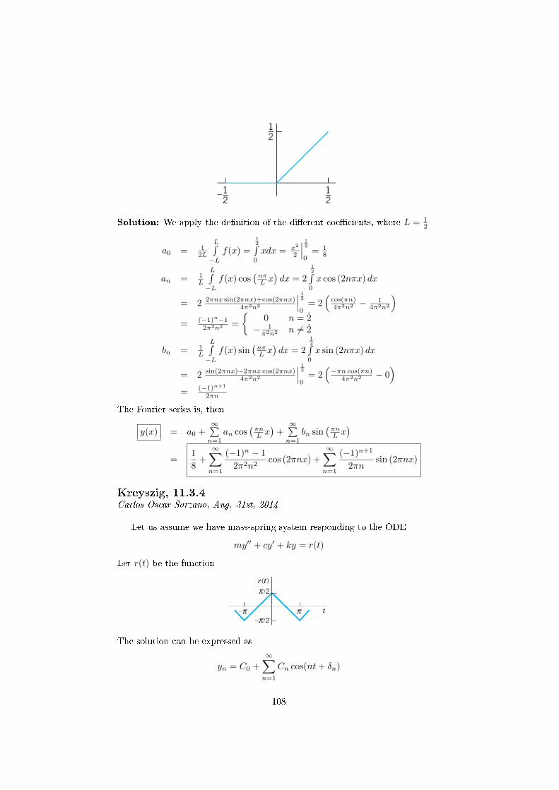
Solution: We apply the de�nition of the di�erent coe�cients, where L = 12

a0 = 12L

L∫−L

f(x) =

12∫0

xdx = x2

2

∣∣∣ 120

= 18

an = 1L

L∫−L

f(x) cos(nπL x)dx = 2

12∫0

x cos (2nπx) dx

= 2 2πnx sin(2πnx)+cos(2πnx)4π2n2

∣∣∣ 120

= 2(

cos(πn)4π2n2 − 1

4π2n2

)= (−1)n−1

2π2n2 =

{0 n = 2

− 1π2n2 n 6= 2

bn = 1L

L∫−L

f(x) sin(nπL x)dx = 2

12∫0

x sin (2nπx) dx

= 2 sin(2πnx)−2πnx cos(2πnx)4π2n2

∣∣∣ 120

= 2(−πn cos(πn)

4π2n2 − 0)

= (−1)n+1

2πn

The Fourier series is, then

y(x) = a0 +∞∑n=1

an cos(πnL x)

+∞∑n=1

bn sin(πnL x)

=1

8+

∞∑n=1

(−1)n − 1

2π2n2cos (2πnx) +

∞∑n=1

(−1)n+1

2πnsin (2πnx)


Let us assume we have mass-spring system responding to the ODE

my′′ + cy′ + ky = r(t)

Let r(t) be the function

The solution can be expressed as

yn = C0 +

∞∑n=1

Cn cos(nt+ δn)

108

What happens if we replace r(t) with its derivative, the rectangular wave?What is the ratio of the new Cn to the old ones?Solution: Let us consider the Fourier series of the input function r(t)

r(t) = c0 +

∞∑n=1

cn cos(nt+ θn)

Its derivative, assuming the series is convergent, can be calculated as

r′(t) =

∞∑n=1

(−cnn sin(nt+ θn)) =

∞∑n=1

cnn cos(nt+ θn + π2 )

Since the parameters m, c and k are constant, then the system is linear. For thisreason, for the input r(t), each harmonic of the input excites the correspondingharmonic of the output, that is

cn → Cn

If now the amplitude of the input is ncn, then amplitude of the output is nCn

ncn → nCn


Find a general solution of the ODE

y′′ + ω2y = sin(αt) + sin(βt)

with ω2 6= α2, β2.Solution: The general solution of the homogeneous equation is

yh = c1 cos(ωt) + c2 sin(ωt)

For the particular solution, we look for a solution of the form

yp = a sin(αt) + b cos(αt) +A sin(βt) +B cos(βt)

y′p = aα cos(αt)− bα sin(αt) +Aβ cos(βt)−Bβ sin(βt)

y′′p = −aα2 sin(αt)− bα2 cos(αt)−Aβ2 sin(βt)−Bβ2 cos(βt)

Substituting into the di�erential equation, we get

[−aα2 sin(αt)− bα2 cos(αt)−Aβ2 sin(βt)−Bβ2 cos(βt)]+ω2[a sin(αt) + b cos(αt) +A sin(βt) +B cos(βt)] =

sin(αt) + sin(βt)

or what is the same

a(ω2 − α2) sin(αt) + b(ω2 − α2) cos(αt)++A(ω2 − β2) sin(βt) +B(ω2 − β2) cos(βt) =

sin(αt) + sin(βt)

109

Equating coe�cients we �nd that

b = B = 0

a =1

ω2 − α2

A =1

ω2 − β2

The general solution of the equation is

y = c1 cos(ωt) + c2 sin(ωt) +1

ω2 − α2sin(αt) +

1

ω2 − β2sin(βt)


Tranformation to Sturm�Liouville form. Show that

y′′ + fy′ + (g + λh)y = 0

takes the form(p(x)y′)′ + (q(x) + λr(x))y = 0

if you set p = exp(∫fdx), q = pg and r = hp. Why would you do such a

transformation?Solution: Let us substitute the proposed functions into the Sturm-Liouvilleform

(py′)′ + (pg + λhp)y = 0

p′y′ + py′′ + (pg + λhp)y = 0

Note that

p′ = f exp

(∫fdx

)= fp

Thenfpy′ + py′′ + (pg + λhp)y = 0

Note that p is never 0, then dividing by p

fy′ + y′′ + (g + λh)y = 0

y′′ + fy′ + (g + λh)y = 0

that is the original ODE.Kreyszig, 11.5.9Carlos Oscar Sorzano, Aug. 31st, 2014

Find the eigenvalues and eigenfunctions of the following Sturm-Liouvilleproblem:

y′′ + λy = 0 y(0) = 0, y′(L) = 0

Solution: We can rewrite the ODE as

(y′)′ + λy = 0

110

with the constraints1y(0) + 0y′(0) = 0

0y(L) + 1y′(L) = 0

That is, this is a Sturm-Liouville problem.If λ < 0, λ = −ν2, then the general solution is

y = c1eνx + c2e

−νx

Imposing the two boundary conditions

y(0) = 0 = c1 + c2y′(L) = 0 = c1νe

νL − c2νe−νL

Its unique solution is c1 = c2 = 0.If λ = 0, then the general solution is

y = c1 + c2x


y(0) = 0 = c1y′(L) = 0 = c2

If λ > 0, λ = ν2, then the general solution is

y = c1 cos(νx) + c2 sin(νx)


y(0) = 0 = c1y′(L) = 0 = −c1 sin(νL) + c2ν cos(νL) = c2ν cos(νL)⇒ νL = π

2 + πk ⇒ ν = π+2πk2L

That is the functions

yν = sin(νx) ν = π+2πk2L

are the eigenfunctions of the Sturm-Liouville problem and their eigenvalues areλ = ν2.Kreyszig, 11.5.11Carlos Oscar Sorzano, Aug. 31st, 2014

Find the eigenvalues and eigenfunctions of the following Sturm-Liouvilleproblem: (

y′

x

)′+ (λ+ 1)

y

x3= 0 y(1) = 0, y(eπ) = 0

(Set x = et).Solution: If we make the change of variable x = et ⇒ t = log(x), then

y′ = dydx = dy

dtdtdx = dy

dt1x = dy

dt e−t

y′′ = dy′

dx = dy′

dtdtdx = d

dt

(dydt e−t)

1x =

(d2ydt2 e

−t − dydt e−t)e−t = d2y

dt2 e−2t − dy

dt e−2t

111

We note that(y′

x

)′=y′′x− y′

x2=

(d2ydt2 e

−2t − dydt e−2t)et − dy

dt e−t

e2t=d2y

dt2e−3t − 2

dy

dte−3t

Then we can rewrite the problem as a function of y(t)(d2y

dt2e−3t − 2

dy

dte−3t

)+ (λ+ 1)ye−3t = 0 y(0) = 0, y(π) = 0

d2y

dt2− 2

dy

dt+ (λ+ 1)y = 0 y(0) = 0, y(π) = 0

We now check if the problem is a Sturm-Liouville problems using Kreyszig 11.5.6with f = −2, g = 1, h = 1. We calculate

p = e∫

(−2)dt = e−2t

q = pg = e−2t

h = hp = e−2t

So, in the Sturm-Liouville form the problem becomes

d

dt

(e−2t dy

dt

)+ (e−2t + λe−2t)y = 0

We go back to the problem

d2y

dt2− 2

dy

dt+ (λ+ 1)y = 0

and look for solutions of the form y = est

s2 − 2s+ (λ+ 1) = 0⇒ s = 1±√−λ

If λ < 0, λ = −ν2, then the general solution is of the form

y = c1es1t + c2e

s2t

with s1 = 1 + ν and s2 = 1− ν. Imposing the two boundary conditions

y(0) = 0 = c1 + c2y(π) = 0 = c1e

s1π + c2es2π

whose unique solution is c1 = c2 = 0.If λ = 0, then the general solution is of the form

y = c1et + c2te

t


y(0) = 0 = c1y(π) = 0 = c1e

π + c2πeπ

whose unique solution is c1 = c2 = 0.

112

If λ > 0, λ = ν2, then the general solution is of the form

y = c1et cos(νt) + c2e

t sin(νt)


y(0) = 0 = c1y(π) = 0 = c2e

π sin(νπ)⇒ ν = k

So, all the functions of the form

y = et sin(kt) = elog x sin(k log(x)) = x sin(k log(x)) k ∈ Z

are eigenfunctions of the Sturm-Liouville problem, and their associated eigen-value is λ = k2.Kreyszig, 11.6.2Carlos Oscar Sorzano, Aug. 31st, 2014

Find the Fourier-Legendre series of the polynomial (x+ 1)2

Solution: The Fourier-Legendre series of the function f is a series expansionof the form

f =

∞∑m=0

〈f, Pm〉‖Pm‖2

Pm(x)

where

‖Pm‖2 =2

2m+ 1

and the Legendre polynomials are given by

P0(x) = 1P1(x) = x

(n+ 1)Pn+1(x) = (2n+ 1)xPn(x)− nPn−1(x)

In particularP2(x) = 1

2 (3x2 − 1)P3(x) = 1

2 (5x3 − 3x)

To perform the Fourier-Legendre expansion, let us perform the followingcalculations ⟨

(x+ 1)2, P0(x)⟩

=1∫−1

(x+ 1)2dx = 83

‖P0‖2 = 22·0+1 = 2⟨

(x+ 1)2, P1(x)⟩

=1∫−1

(x+ 1)2xdx = 43

‖P1‖2 = 22·1+1 = 2

3⟨(x+ 1)2, P2(x)

⟩=

1∫−1

(x+ 1)2 12 (3x2 − 1)dx = 4

15

‖P2‖2 = 22·2+1 = 2

5⟨(x+ 1)2, P3(x)

⟩=

1∫−1

(x+ 1)2 12 (5x3 − 3x)dx = 0

‖P3‖2 = 22·3+1 = 2

7

113

Actually, since f is a polynomial of degree 2, and Legendre polynomials area basis of polynomials in the domain [−1, 1], we have that all coe�cients form ≥ 3 are 0 (

⟨(x+ 1)2, Pm(x)

⟩= 0).

Finally, the Fourier-Legendre expansion is

(x+ 1)2 =〈(x+1)2,P0(x)〉

‖P0‖2 P0 +〈(x+1)2,P1(x)〉

‖P1‖2 P1 +〈(x+1)2,P2(x)〉

‖P2‖2 P2

=83

2 +4323

x+41525

12 (3x2 − 1)

=4

3+ 2x+

2

3

1

2(3x2 − 1)

Kreyszig, 11.9.6Carlos Oscar Sorzano, Dec. 19th, 2014

Find the Fourier transform of f(x) = e−|x| (−∞ < x <∞) by integration.Solution: The de�nition of the Fourier transform is

f(ω) =1√2π

∞∫−∞

f(x)e−iωxdx

Substituting in this formula the value of f , we have

f(ω) = 1√2π

∞∫−∞

f(x)e−iωxdx

= 1√2π

∞∫−∞

e−|x|e−iωxdx

= 2√2π

∞∫0

e−xe−iωxdx

= 2√2π

∞∫0

e−(1+iω)xdx

= 2√2π

e−(1+iω)x

−(1+iω)

∣∣∣∞0

=√

2π

11+iω

8 Chapter 12


Verify that the functionu = x2 + t2

is a solution of the wave equation

utt = c2uxx

for a suitable c.

114

Solution: Let us calculate the di�erent partial derivatives needed to substitutein the wave equation

ut = 2tutt = 2ux = 2xuxx = 2

The wave equation states2 = c22

which is true for c = 1. In Matlab:[x,t]=meshgrid(-2:0.15:2,0:0.15:2);

u=x.�2+t.�2;

surfc(x,t,u)

xlabel('x'); ylabel('t'); zlabel('u')

−2−1

01

2

0

0.5

1

1.5

20

2

4

6

8

xt

u


Verify that the function

u = sin(at) sin(bx)

is a solution of the wave equation

utt = c2uxx

for a suitable c.Solution: Let us calculate the di�erent partial derivatives needed to substitutein the wave equation

ut = a cos(at) sin(bx)utt = −a2 sin(at) sin(bx)ux = b sin(at) cos(bx)uxx = −b2 sin(at) sin(bx)

115

The wave equation states

−a2 sin(at) sin(bx) = c2(−b2 sin(at) sin(bx))

which is true for c = a2

b2 . In Matlab:[x,t]=meshgrid(-3*pi:0.1:3*pi,0:0.1:3*pi);

u=sin(t).*sin(x);

surfc(x,t,u)

xlabel('x'); ylabel('t'); zlabel('u')

−10−5

05

10

0

5

10−1

−0.5

0

0.5

1

xt

u


Solveuy + y2u = 0

Solution: Since the PDE is only depending on y, we can treat x as if it werea parameter, then we can solve the PDE as if it were an ODE on y

uy = −y2u

du

u= −y2

log |u| = −y3

3+ C(x)

u = C(x)exp

(−y

3

3

)Kreyszig, 12.4.11

116


Find the type, transform to normal form and solve

uxx + 2uxy + uyy = 0

Solution: The prototypical equation for the method of characteristics is of theform

Auxx + 2Buxy + Cuyy = F (x, y, u, ux, uy)

which corresponds to the equation in the problem with

A = B = C = 1

Consequently,AC −B2 = (1)(1)− 12 = 0

that is, the PDE is a parabolic PDE. Its characteristic equation is

A(y′)2 − 2By′ + C = 0

(y′)2 − 2y′ + 1 = 0

(y′ − 1)2 = 0

whose solution isy = c1 + x⇒ Ψ(x, y) = y − x = c1

We now do the change of variables

v = x

w = y − x

The standard form of a parabolic PDE is

uww = 0

Integrating in w we haveuw = φ(w)

Integrating again in w

u =

∫φ(w)dw + ψ(w) = ζ(w) + ψ(w) = η(w)


u = η(y − x)

being η any function.Kreyszig, 12.4.19Carlos Oscar Sorzano, Aug. 31st, 2014

Longitudinal Vibrations of an Elastic Bar or Rod. These vibrationsin the direction of the x-axis are modeled by the wave equation

utt = c2uxx

117

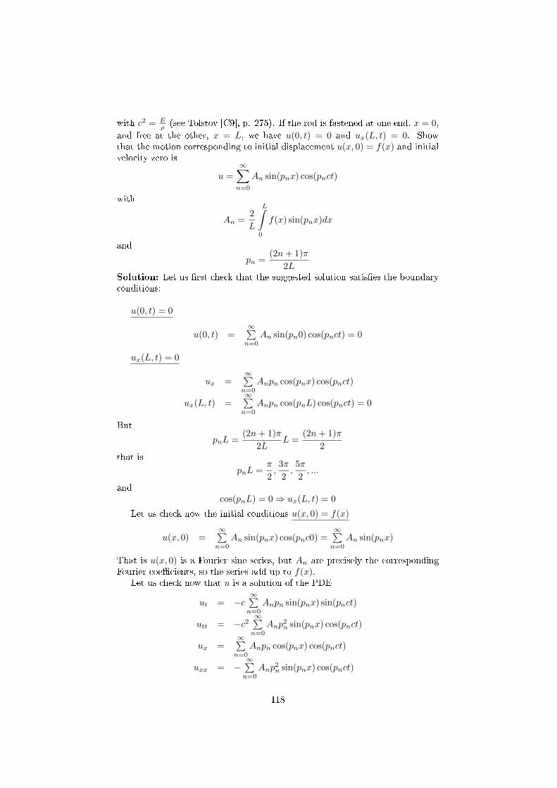
with c2 = Eρ (see Tolstov [C9], p. 275). If the rod is fastened at one end, x = 0,

and free at the other, x = L, we have u(0, t) = 0 and ux(L, t) = 0. Showthat the motion corresponding to initial displacement u(x, 0) = f(x) and initialvelocity zero is

u =

∞∑n=0

An sin(pnx) cos(pnct)

with

An =2

L

L∫0

f(x) sin(pnx)dx

and

pn =(2n+ 1)π

2LSolution: Let us �rst check that the suggested solution satis�es the boundaryconditions:

u(0, t) = 0

u(0, t) =∞∑n=0

An sin(pn0) cos(pnct) = 0

ux(L, t) = 0

ux =∞∑n=0

Anpn cos(pnx) cos(pnct)

ux(L, t) =∞∑n=0

Anpn cos(pnL) cos(pnct) = 0

But

pnL =(2n+ 1)π

2LL =

(2n+ 1)π

2that is

pnL =π

2,

3π

2,

5π

2, ...

andcos(pnL) = 0⇒ ux(L, t) = 0

Let us check now the initial conditions u(x, 0) = f(x)

u(x, 0) =∞∑n=0

An sin(pnx) cos(pnc0) =∞∑n=0

An sin(pnx)

That is u(x, 0) is a Fourier sine series, but An are precisely the correspondingFourier coe�cients, so the series add up to f(x).

Let us check now that u is a solution of the PDE

ut = −c∞∑n=0

Anpn sin(pnx) sin(pnct)

utt = −c2∞∑n=0

Anp2n sin(pnx) cos(pnct)

ux =∞∑n=0

Anpn cos(pnx) cos(pnct)

uxx = −∞∑n=0


118

The PDE statesutt = c2uxx

−c2∞∑n=0

Anp2n sin(pnx) cos(pnct) = c2

(−∞∑n=0


)The equation above is obviously true, so the proposed function is a solution ofthe PDE and it sati�es the boundary conditions.Kreyszig, 12.6.11Carlos Oscar Sorzano, Aug. 31st, 2014

Show that for the completely insulated bar, ux(0, t) = 0, ux(L, t) = 0 andu(x, 0) = f(x) and separation of variables the solution of the heat equation

ut = c2uxx

gives the solution

u(x, t) = A0 +

∞∑n=1

An cos(nπxL

)e−( cnπL )

2t

with

A0 =1

L

L∫0

f(x)dx

An =2

L

L∫0

f(x) cos(nπxL

)dx

Solution: Let us �rst check that the suggested solution satis�es the boundaryconditions:

ux(0, t) = 0

ux = −∞∑n=1

AnnπL sin

(nπxL

)e−( cnπL )

2t

ux(0, t) = −∞∑n=1

AnnπL sin

(nπ0L

)e−( cnπL )

2t = 0

ux(L, t) = 0

ux(L, t) = −∞∑n=1

AnnπL sin

(nπLL

)e−( cnπL )

2t = 0

because

sin

(nπL

L

)= sin(nπ) = 0

Let us check now the initial conditions u(x, 0) = f(x)

u(x, 0) = A0 +∞∑n=1

An cos(nπxL

)e−( cnπL )

20

= A0 +∞∑n=1

An cos(nπxL

)119

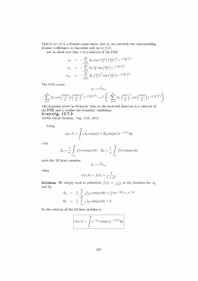
That is u(x, 0) is a Fourier cosine series, but An are precisely the correspondingFourier coe�cients, so the series add up to f(x).

Let us check now that u is a solution of the PDE

ut = −∞∑n=1

An cos(nπxL

) (cnπL

)2e−( cnπL )

2t

ux = −∞∑n=1

AnnπL sin

(nπxL

)e−( cnπL )

2t

uxx = −∞∑n=1

An(nπL

)2cos(nπxL

)e−( cnπL )

2t

The PDE statesut = c2uxx

−∞∑n=1

An cos(nπxL

)(cnπL

)2

e−( cnπL )2t = c2

(−∞∑n=1

An

(nπL

)2

cos(nπxL

)e−( cnπL )

2t

)The equation above is obviously true, so the proposed function is a solution ofthe PDE and it sati�es the boundary conditions.Kreyszig, 12.7.3Carlos Oscar Sorzano, Aug. 31st, 2014

Using

u(x, t) =

∞∫0

(Ap cos(px) +Bp sin(px))e−c2p2tdp

with

Ap =1

π

∞∫−∞

f(v) cos(pv)dv Bp =1

π

∞∫−∞

f(v) sin(pv)dv

solve the 1D heat equationut = c2uxx

when

u(x, 0) = f(x) =1

1 + x2

Solution: We simply need to substitute f(x) = 11+x2 in the formulas for Ap

and Bp

Ap = 1π

∞∫−∞

11+v2 cos(pv)dv = 1

π (πe−|p|) = e−|p|

Bp = 1π

∞∫−∞

11+v2 sin(pv)dv = 0

So the solution of the 1D heat problem is

u(x, t) =

∞∫0

e−|p| cos(px)e−c2p2tdp

120

problems differential equations

Documents

ex sinx ex cosxcosxexdx

ex sinx ex cosxi1

ex sinxcosx2finallyy

ex sinxsinxexdx

ex cosxdxand

ex cosxby

ex cosxdxlets

ex cosxsolution