problem whose solutions can be 'ranked'yfwang/courses/cs130b/notes/greedy.pdf · select:...

Greedy Methods

Data Structures and Algorithms II

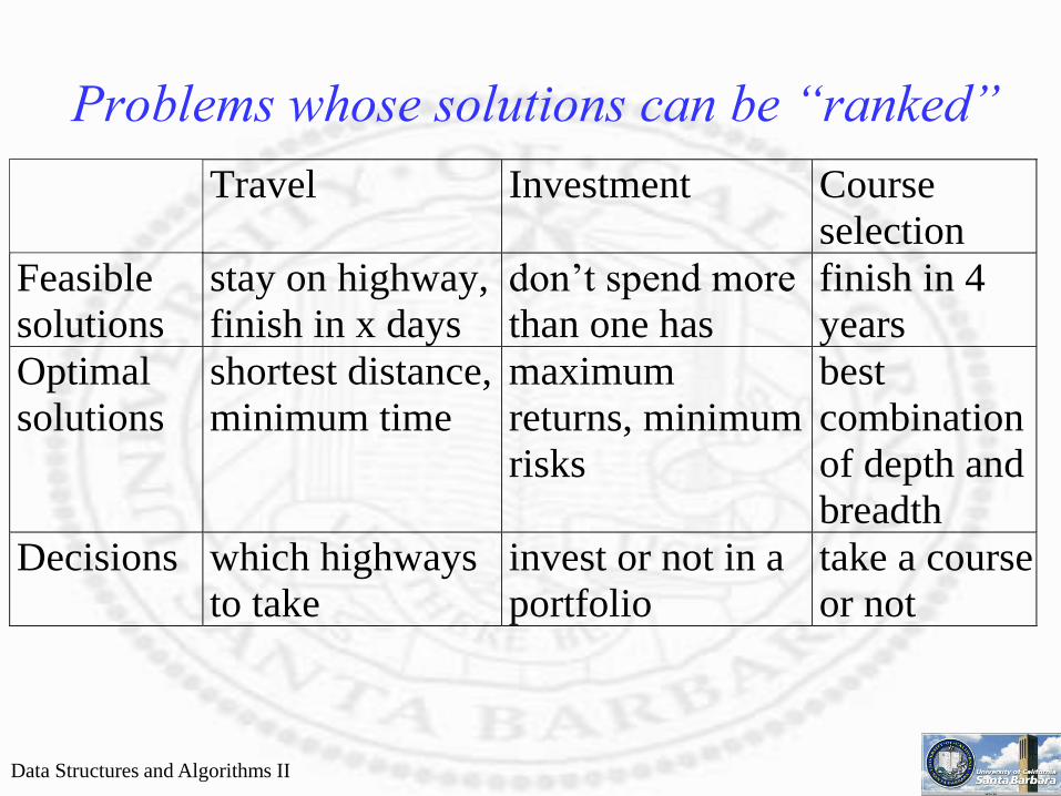
Problems whose solutions can be “ranked”

Travel Investment Course

selection

Feasible

solutions

stay on highway,

finish in x days

don’t spend more

than one has

finish in 4

years

Optimal

solutions

shortest distance,

minimum time

maximum

returns, minimum

risks

best

combination

of depth and

breadth

Decisions which highways

to take

invest or not in a

portfolio

take a course

or not


Decisions can be made

one at a time, without backtracking

Greedy method

Which decisions to make next?

How to guarantee optimality?

Try many (all) possible combinations and

choose one which is the best

Dynamic programming

How to test multiple solutions efficiently?


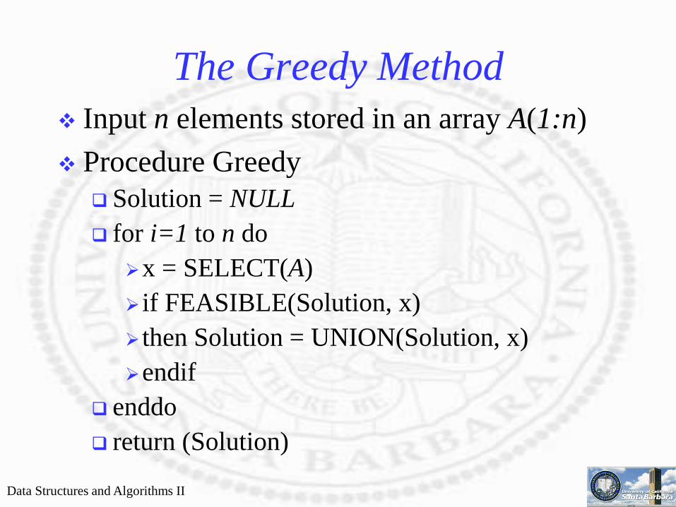
The Greedy Method

Input n elements stored in an array A(1:n)

Procedure Greedy

Solution = NULL

for i=1 to n do

x = SELECT(A)

if FEASIBLE(Solution, x)

then Solution = UNION(Solution, x)

endif

enddo

return (Solution)


A sequence of n decisions w.r.t n inputs

SELECT: select one of the remaining

decisions to make according to some

optimization measure

once a decision is made, it will not become

invalid at a later time

optimization should be based on the partial

solutions built so far

FEASIBLE: whether the partial solution

satisfies some preset constraints


Strategy: construct feasible solutions one

step at a time which optimize (minimize or

maximize) a certain objective function

Make the obvious decisions first!

Then try to show it is indeed optimal!


Knapsack problem

Input:

a set of n objects

a knapsack of capacity M

Output: fill the knapsack to maximize the

total profit earned

Feasibility constraint:

Objective function:

( , ) ,...,P W i ni i 1

W X Mi ii

n

1

max P X Xi ii

n

i

1

0 1


Example

n M

P P P

W W W

X X X W X P Xi i

i

n

i i

i

n

3 20

25 24 15

18 1510

12

150 20 28 2

02

31 20 31

0 11

220 315

1 2 3

1 2 3

1 2 3

1 1

,

( , , ) ( , , )

( , , ) ( , , )

( , , )

( , , ) .

( , , )

( , , ) .

largest increase in profit

smallest increase in weight

largest increase in profit to

weight ratio

( , , ) ( . , . , .P

W

P

W

P

W

1

1

2

2

3

3

139 16 15)


For all three algorithms

decisions are made one object at a time

the ordering is determined by some

optimization measure

Largest increase in profit

Include the remaining object of the largest profit

Smallest increase in weight

Include the remaining object of the smallest weight

Largest increase in profit/weight

Include the remaining object of the largest profit/weight

never backtrack

all greedy algorithms

not all guarantee optimal


Proposition: Greedy selection based on

maximizing profit to weight ratio gives the

optimal result

General proof strategy:

Assume that the greedy solution is

Assume that the optimal solution is

Then they better be different

Transform Y into X without decreasing the

profit of Y

X X X Xn ( , ,..., )1 2

Y Y Y Yn ( , ,..., )1 2


Proof:

Assume P

W

P

W

P

W

n

n

1

1

2

2

...

1 1 …. 1 0 0 0 …. 0 01 Greedy (X)

Optimal (Y)

0 1 X j

– Let k be the first index where X and Y differ

( ) &

( )

( ) & & ,

i k j X Y X Y X

ii k j if Y X then WY M Y X

iii k j X Y X Y WY M not possible

k k k k k

k k i i k k

k k k k i i

1

0 0


New optimal (Z)

Optimal (Y)

Y Xk k

n

i

ii

n

ki k

kiiikkk

n

i

ii

n

ki

i

i

iiik

k

kkk

n

i

ii

n

ki

iiikkk

n

i

ii

n

i

ii

PY

W

PWZYWYZPY

WW

PZYW

W

PYZPY

PZYPYZPYPZ

1

11

11

111

in weight decreasein weight increase

})(){(

)()(

profit of decreaseprofit of increaseY ofprofit

)()(


Z is also an optimal solution

Either Z=X (Done)

Or not (Repeat the above procedure until Z=X)


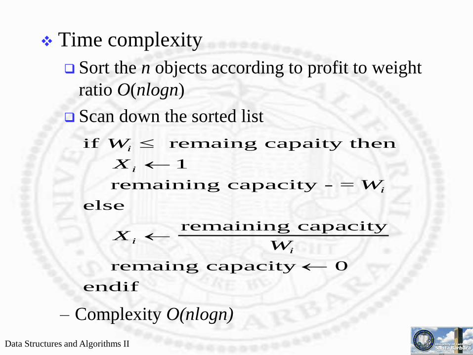
Time complexity

Sort the n objects according to profit to weight

ratio O(nlogn)

Scan down the sorted list

if remaing capaity then

remaining capacity - =

else

remaining capacity

remaing capacity 0

endif

W

X

W

XW

i

i

i

i

i

1

– Complexity O(nlogn)


Optimal Storage on Tape

Input:

A set of n programs of different length

A computer tape of length L

Output:

A storage pattern which minimizes the total

retrieval time (TRT)

before each retrieval, head is repositioned at the front

TRT l I i i iik jj n

nk

111 2, ,...


Objective function: minimize TRT


Example

l Lik n

k1

n l l l L

ordering

i i iTRT

3 510 3 20

1 2 3 5 5 10 5 10 3 38

1 3 2 5 5 3 5 3 10 31

2 1 3 10 10 5 10 5 3 43

2 31 10 10 3 10 3 5 41

31 2 3 3 5 3 5 10 29

3 2 1 3 3 10 3 10 5 34

1 2 3

1 2 3

,( , , ) ( , , ),

( )

, ,

, ,

, ,

, ,

, ,

, ,

, ,


SELECT: Select the program to store next

which minimizes the increase in TRT

TRT l

TRT l TRT l

TRT TRT l l l

old ik jj r

new i old ik rk jj r

new old ik r

ik r

r

k

k k

k k

11

1 111 1

1 1 11

i1 i2 ir ir1

fixed Currently shortest

program

Proof strategy

follow the same principle as in knapsack

problem

there is a greedy solution

there is an optimal solution

they are different

line them up and they better differ in some storage

locations

then make them the same (by swapping)

prove that the swapping does not reduce the

optimality


Front

Optimal

Greedy

i1 i2 ir

siir

sr ii

si

Swap ir and is in the optimal solution


Intuitively

a b

Front

• For programs stored in

– retrieval does not scan through either a or b

– ordering of a and b not important


– retrieval scans through both a and b

– ordering of a and b not important


– retrieval scans through a but not b

– ordering of a and b is important


Proposition: The storage pattern with

nondecreasing length order produces the

smallest TRT

l l

l l

l l l

l l l l

l n l n l l

n k l

i

k jj n

i

i i

i i i

i i i i

i i i i

i

k n

k

n

n

k

11

1

1

1 2

1 2 3

1 2 3

1 2 31 2

1

... ... ...

...

( ) ( ) ...

( )

= n


If prog. a and prog. b are out of order, then

swap them should reduce the TRT

TRT n k l n a l n b l

TRT n k l n a l n b l

TRT TRT n a l l n b l l

b a l l

old i ikk ak b

i

new i ikk ak b

i

old new i i i i

i i

k a b

k b a

a b b a

a b

( ) ( ) ( )

( ) ( ) ( )

( )( ) ( )( )

( )( )

1 1 1

1 1 1

1 1

0

• Time complexity: O(nlogn) for sorting


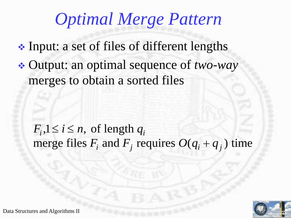
Optimal Merge Pattern

Input: a set of files of different lengths

Output: an optimal sequence of two-way

merges to obtain a sorted files

F i n q

F F O q qi i

i j i j

, ,

( )

1

of length

merge files and requires time


Examplen q q q

ordering

3 30 20 101 2 3,( , , ) ( , , )

cost

1,2,3 50 + 60 = 110

1,3,2 40 + 60 = 100

2,1,3 50 + 60 = 110

2,3,1 30 + 60 = 90

3,1,2 40 + 60 = 100

3,2,1 30 + 60 = 90

• Programs (files) stored on a tape (already merged together)

may affect the access times (the merge times) of new

programs (files) to be stored (merged)

• SELECT: At each step, merge two smallest files

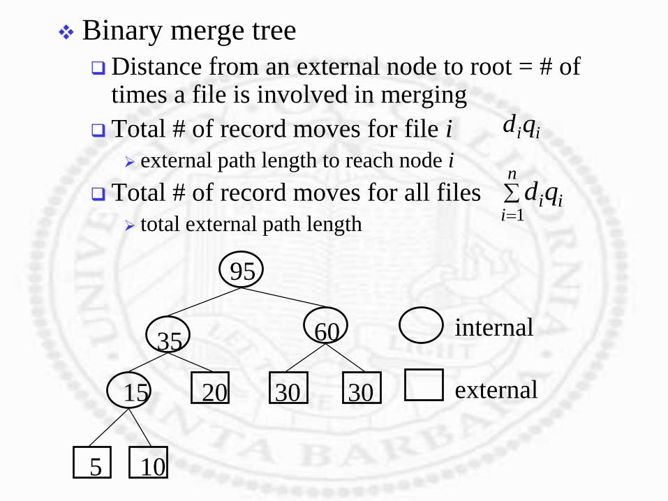
Binary merge tree

Distance from an external node to root = # of times a file is involved in merging

Total # of record moves for file i

external path length to reach node i

Total # of record moves for all files

total external path length

5 10

20 30 3015

35 60

95

internal

external

d qi ii

n

1

d qi i


Huffman Code

For data compression to save storage space

and transmission bandwidth

ASCII code uses fixed-length 8

bits/character code words, O(8n) for storage

and transmission

Huffman codes uses variable-length code

words depending on the frequency of

occurrence


Example

a b c d e f

Frequency

(thousands)

45 13 12 16 9 5

Fixed-length 000 001 010 011 100 101

Variable-length 0 101 100 111 1101 1100

bits000,2244000,54000,93000,16

3000,123000,131000,45length-variable

bits000,300300

0,100lengthfixed


Prefix codes

no codeword is a prefix of some other

codeword

1010

1010001

… 110 …. 1010 …

codeword a

codeword b

codeword a?

or beginning of codeword b?


a:45d:16 b:13c:12e:9f:5

a:45

e:9f:5

14

10

a:45

e:9f:5

14

10

d:16 b:13c:12

d:16

b:13c:12

25

10


a:45

e:9f:5

14

10

d:16

b:13c:12

25

10

30

10

a:45

e:9f:5

14

10

d:16

b:13c:12

25

10

30

10

0

1

55


a:45

e:9f:5

141 0

d:16

b:13c:12

251

0

301

0

0

1

55

0

1

100

Huffman code

Distance from an external node to root = # of bits in the code word

Total effort of sending i

external path length to reach node i

Total effort of sending all alphabets

total external path length

d qi ii

n

1

d qi i

a:45

e:9f:5

141 0

d:16

b:13c:12

251

0

301

0

01

55

0

1

100

An Important Fact

Using Huffman-tree rules, nodes that are

merged first must have a longer path to the

root than nodes that are merged later

2,,21 jipppp ji

lmax

No node can be merged more than once

before p1+p2 is involved again

An Important Fact (cont.)

An iteration:

Between two successive merges involve p1

In an iteration

No node can be involved in more than one

merge

No node can increase in path length more than

p1

Hence, p1 must have the longest path length


Proposition: Huffman construction

minimizes the expected codeword length p l

p

l

i ii

n

i

i

1

probability of occurance

codeword length

• Proof:

Optimal prefix-code tree Huffman prefix-code tree

transform without increasing

expected codeword length

Assume that p p pn1 2 ...

Optimal prefix-code tree

pip j

p1

p2

pi

p j

p1 p2

l1

l2

lmax

2211maxmax

,,2,11

plplplpl

lplp

ji

jik

kk

n

k

kk

ji

jik

kk

n

k

kk

plplplpl

lplp

212max1max

,,2,11

'

0))(())((

'

22max11max

212max1max2211maxmax

11

ppllppll

plplplplplplplpl

lplp

ji

jiji

n

k

kk

n

k

kk

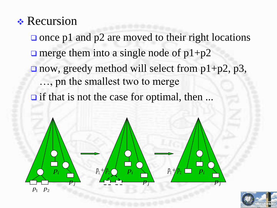
Recursion

once p1 and p2 are moved to their right locations

merge them into a single node of p1+p2

now, greedy method will select from p1+p2, p3,

…, pn the smallest two to merge

if that is not the case for optimal, then ...

pi

p j

p1 p2

pi

p j

21 pp pi

p j

21 pp


Time complexity

with n alphabets to code, exactly n-1 merges

are needed

for each merge

find an least-frequently-used alphabet

find the next least-frequently-used alphabet

merge

put merged subtrees back into the list of subtrees

priority queue (heap) is ideal for this operation

O(n) steps of detelemin and insert (O(logn))

O(nlogn)


Minimum-Cost Spanning Tree

Input: G=(V,E), an undirected, labeled

graph

Output: T=(V,E’), a subgraph of G

includes all the vertices

is a tree

the sum of labels (costs) of all tree branches is

minimum among all spanning trees

}(Spanning tree)


Objective function:

Feasibility constraint: a tree containing all

vertices

Example

cos ( )t eii SP

16

5

6

10

18

1911

21

33 14

16

5

6

18

11

16

10

18

21

33

cos ( )t eii SP

56

cos ( )t eii SP

98


SELECT: At each step, choose an edge with

minimum cost (optimality) such that

(feasibility):

the partial solution is always a tree (Prim)

the partial solution has potential of becoming a

tree (no cycles, but not necessarily connected)

(Kruskal)


Prim’s algorithm

First step: select a minimum cost edge,

include it in the solution

Other steps: select an edge (u,v), u in U and

v in V-U, until all vertices are counted for

UV-U

Select one

Example

A

B C

D E

F

G

611

14

2

2

1

22

4

A

B C

D E

F

G

11

2

1

2 1

2

A

B C

D E

F

G

61

2

A

B C

D E

F

G

611

2 2

A

B C

D E

F

G

611

42

A

B C

D E

F

G

611

42 2

1

2

4

4 4

: set U


2

A

B C

D E

F

G

611

42

1

4

2

A

B C

D E

F

G

611

2

1

2 1

A

B C

D E

F

G

11

2

1

2 1

: set U


A B C D E F G

A A A A A A

B B B A A

B B A A

D D A

D A

E

( , ) ( , ) ( , ) ( , ) ( , ) ( , )

( , ) ( , ) ( , ) ( , ) ( , )

( , ) ( , ) ( , ) ( , )

( , ) ( , ) ( , )

( , ) ( , )

( , )

1 2 6

1 2 4 2 6

2 4 2 6

2 1 6

2 6

1

Cost Cost Cost new i

Closest Cost Cost new i new Closet

i i

i i i

min( , ( , ))

( ( , ))? :

Step

1

2

3

4

5

6

Cost update

Nearest neighbor update


Proposition: Prim’s algorithm finds MCST

Proof:

U V-U

e

e’

– Again, there are two solutions, PRIM and MCST

– They better differ, and MCST has a lower cost

– In the construction of PRIM, if an edge e is considered

– It is in MCST, ok, continue (cannot be forever)

– If it is not in MCST, then ….


Proposition: Prim’s algorithm finds MCST

Proof: U V-U

e

e’

– Let U be the subgraph (tree) considered so far

– Let V-U be the remaining part, then

– There must be at least one edge (e’) chosen between U

and V-U in MCST

• Prim’s algorithm selects the minimum cost one (e)

• e’ can be replaced by e in the MCST


No cycle U has no cycle

V-U has no cycle

Between U and V-U cannot has cycle w. a single path e

Still connected U is connected

V-U is connected

U and V-U connected through either e or e’

The same number of edges => it is a spanning tree

A tree of a smaller cost

U

e

e’

V-U


Time complexity

Totally n vertices have to be connected

Each time an edge is added, one additional vertex

is accounted for

Loop through n-1 times

Through each loop

Select the edge of a minimum cost from U to V-U

Update the nearest vertex and cost for vertices in V-U’

O(n-i)

O(n-i)

( ) ( )n i O ni

n

1

1

2


Kruskal’s algorithm

B C

D E

F

G

611

14

2

2

1

22

4

A

B

1A

B C

11

A

B C

11

A

D

F

1

Edge Cost

AB

BC

DF

EG

AF

BD

DE

EF

BE

CE

AG

1

1

1

1

2

2

2

2

4

4

6

( )

( )

( )

( )

( )

B C

11

A

D

F

1

E

G

1

B C

11

A

D

F

1

E

G

12

B C

11

A

D

F

1

E

G

12 2

Edge Cost

AB

BC

DF

EG

AF

BD

DE

EF

BE

CE

AG

1

1

1

1

2

2

2

2

4

4

6

( )

( )

( )

( )

( )


Proposition: Kruskal’s algorithm find MCST

Proof:

ee

ii

Ee

Ee

Ee

Ee

Ee

MST

T

sKruskal

T

33

22

11

'

'

first index the two

solutions differ

ejiECosteCost ji )()(


Including in MCST creates a cycle

Not all edges in the cycle belongs to T (Kruskal’s)

At least one of them must have a higher costs

Remove that high-cost edge breaks the cycle and

maintain the tree structure

ei

ei

Ei1Ei2

Eik

ei

Ei1Ei2

Eik

Time complexity Total e edges are considered in order of

nondecreasing cost Use partially-ordered tree (heap) to represent edges

Construction O(e log e)

Deletemin O(e log e)

At each step, remove edge with a minimum cost and check to see whether it creates a cycle if included

Use Union-and-Find tree

Initially each vertex in a set by itself

Inclusion of an edge, join the sets containing the edge’s two end points

Edges are not included if the two end points are in the same set

O(e log e)

Single-Source Shortest Path

Input:

G=(V,E), an directed, labeled graph

A source vertex

Output:

The shortest path, from source to every other

vertices in the graph, if one exists

Possible Greedy Strategies

Exploring a maze where you cannot see

beyond the first turn

Extremely greedy: with no memory, go

where the path leads you (good paths can

turn bad at any instance)

Cautiously greedy: with memory, go where

the shortest path encountered so far

(backtracking to the path necessary)

Greedy Selection

1. Visited set = {s}

2. From visited set, find all 1-distance (direct edge) neighbors

3. Visit the one with the shortest distance: n

4. Enlarge visited set = visited set U {n}

5. Update distances to the remaining vertices

1. Go through original visited set

2. Go through n

6. Go back to 2

If (dist(w)>dist(n)+cost(n,w)) {

dist(w) = dist(n)+cost(n,w);

previous_neighbor = n;

}

Complexity: O(n2)

Comparison

Prim’s MCST

Two groups

Already in ST (U)

Not yet in ST (V-U)

Update

Find the min edge from

U to V-U

Build table of partial

solutions: O(n) steps,

<O(n) updates O(n2)

Dijkstra’s shortest path

Two groups

Already found path to

Not yet found path to

Update

Find the shortest path from

U to V-U

Build table of partial

solutions: O(n) steps,

<O(n) updates O(n2)

Cost Cost Cost new i

Closest Cost Cost new i new Closet

i i

i i i

min( , ( , ))

( ( , ))? :




}

Initially You cannot go to blue through dashed green and

then circle back with a lower cost

Next Step Dashed blue: reached by blue only

Dashed green: reached by green only

Dashed cyan: reached by both green

and blue

One of the dashed blue, green, or cyan will be visited next (i.e., the shortest

path to the visited node is determined greedily)

Is that possible to go through other dashed blue, green, or cyan and circle back

to the visited node with a shorter path?

Case one: Dashed green is selected

Other dashed green: cannot be shorter

Dashed blue: cannot be shorter

Dashed cyan: cannot be shorter

Case two: Dashed blue is selected

Dashed green: cannot be shorter

Other dashed blue: cannot be shorter

Dashed cyan: cannot be shorter

Case three: Dashed cyan is selected

Dashed green: cannot be shorter

Dashed blue: cannot be shorter

Other dashed cyan: cannot be shorter

Induction

Assume that the (current) shortest path to neighbors right outside the wall (one distance away) has been found




}

Induction




}

One more node is

added

Three things can happen for a node still outside

the wall (the envelop) after a new node is added

Not reached by the new node

The current best path didn’t change

Reached by the new node but not any node in the

previous envelop

The current best path must be the one via the new node

Reached by the new node and also nodes in the

previous envelop

The update process should record the best between the two

Hence, when “the best of the best” is chosen to

go out the wall, one cannot jump through other

paths on the wall and circle back to get a better

result


Job Sequencing with Deadlines

Input:

a set of n jobs, each with a deadline and a profit

if completed before deadline

one machine to execute all the jobs

each job takes one unit of time

Output:

a subset of jobs, each completed before

deadline, with maximum profit


Objective function:


Example:

max Pii J

n P P P P

d d d d

4 100 10 15 27

2 1 2 1

1 2 3 4

1 2 3 4

,( , , , ) ( , , , )

( , , , ) ( , , ,

feasible schedule profit

(1,2) 2,1 110

(1,3) 1,3 or 3,1 115

(1,4) 4,1 127

(2,3) 2,3 25

(3,4) 4,3 42

(1) 1 100

(2) 2 10

(3) 3 15

(4) 4 27


SELECT: select the job with maximum

profit subject to the constraint that the

resulting schedule is still feasible

J P

Initially

not feasible

not feasible

ii J

0

1 1 100

4 1 4 127

3 1 4 127 1 4 3

2 1 4 127 1 4 2

( )

( , )

( , ) ( , , )

( , ) ( , , )


(Q1) How to determine if J is feasible?

(Q2) Is greedy algorithm optimal?

(Q1) If J={1,2,3,…,k}

try all possible (k!) permutations (schedules)

and see whether at least one of them allows all

jobs to be finished before their deadlines

intuitively, jobs with earlier deadline (more

urgent) should be performed first

check the permutation * ( , ,..., )

...

i i i

d d d

k

i i ik

1 2

1 2


Proposition: J={1,2,…,k} is feasible if and

only if is feasible

Proof:

If is feasible, then J={1,2,…,k} is feasible

(by definition)

If J={1,2,…,k} is feasible, then

*

*

' timea b

backward moved becan i

forward moved becan j

order ofout

deadline before completed job

bdd

abd

dd

bd

ad

ji

j

ji

j

i

i j


Proposition: The greedy method produces a

schedule with the maximum profit

Proof:

Two different solutions: optimal and greedy

Jobs that are in both optimal and greedy

make sure that they are scheduled at the same time

Jobs that are in one but not the other

change them into ones in greedy without decreasing

profit

The process continues until two solutions are

equal

For jobs that are in both

the job is scheduled the same in both

the job is scheduled earlier in optimal

the job is scheduled earlier in greedy

Again, change optimal to greedy

I(greedy)

J(optimal)

a

a b

time

I(greedy)

J(optimal)

a

ba time

For jobs that are different

I’ and J’ are such that jobs common to both are

scheduled at the same slot

I’(greedy)

J’(optimal)b

timea

P Pa b if b has a larger profit

and is feasible, it will appear in

the greedy solution

time

– Replace b with a in the optimal solution will

not decrease the profit

Finally

Can it be that greedy solution still does

more jobs than optimal?

No, optimal will not be optimal then

Can it be that optimal solution does more

jobs than greedy?

No, if such a job is feasible, how come greedy

solution doesn’t include it?


Time complexity

Sort jobs according to nondecreasing profit

O(nlogn)

Consider n jobs in turn

for each job, insert the job into the partial solution

using its deadline O(i)

check whether the new solution is still feasible O(i)

O n( )2


Greedy Method as Heuristics

For problems whose solutions are found by

“try-all-possibilities,” an optimal solution is

difficult to compute for large problem size

Greedy method can usually produce a “very

good” solution at a fraction of the cost


Example: Traveling salesperson’s problem

Input: a fully connected, labeled undirected

graph

Output: a tour (a simple cycle including all

vertices) whose edge weights are minimum.

Greedy method:

A variant of Kruskal’s algorithm

Consider edges in nondecreasing cost

The edge under consideration, together with all

edges already selected:

do not cause a vertex to have a degree of three or more

do not form a cycle, unless the number of edges equals to

that of vertices


(0,0)

(4,3)

(1,7) (15,7)

(15,4)

(18,0)

1

2

3

45 6

7

8

9

10

Greedy solution

5,6 rejected: cycle

7,8 rejected: vertex

degree larger than 2

cost = 49.73

Optimal solution

cost = 48.39

problem whose solutions can be 'ranked'yfwang/courses/cs130b/notes/greedy.pdf · select:...

Documents