Astronomy&Astrophysics

A&A 613, A54 (2018)https://doi.org/10.1051/0004-6361/201732225© ESO 2018

Probing the use of spectroscopy to determine the meteoriticanalogues of meteors?

A. Drouard1,3, P. Vernazza1, S. Loehle2, J. Gattacceca3, J. Vaubaillon4, B. Zanda4,5, M. Birlan4,7, S. Bouley4,6,F. Colas4, M. Eberhart2, T. Hermann2, L. Jorda1, C. Marmo6, A. Meindl2, R. Oefele2, F. Zamkotsian1, and F. Zander2

1 Aix-Marseille Université, CNRS, LAM (Laboratoire d’Astrophysique de Marseille) UMR 7326, 13388 Marseille, Francee-mail: alexis.drouard@lam.fr

2 IRS, Universität Stuttgart, Pfaffenwaldring 29, 70569 Stuttgart, Germany3 Aix-Marseille Université, CNRS, IRD, Coll France, CEREGE UM34, 13545 Aix en Provence, France4 IMCCE, Observatoire de Paris, Paris, France5 Université Pierre et Marie Curie Paris, IMPMC-MNHN, Paris, France6 GEOPS, Univ. Paris-Sud, CNRS, Université Paris-Saclay, Rue du Belvédère, Bât. 509, 91405 Orsay, France7 Astronomical Institute of Romanian Academy, 5 Cutitul de Argint Street, 040557 Bucharest, Romania

Received 2 November 2017 / Accepted 26 January 2018

ABSTRACT

Context. Determining the source regions of meteorites is one of the major goals of current research in planetary science. Whereasasteroid observations are currently unable to pinpoint the source regions of most meteorite classes, observations of meteors with cam-era networks and the subsequent recovery of the meteorite may help make progress on this question. The main caveat of such anapproach, however, is that the recovery rate of meteorite falls is low (<20%), implying that the meteoritic analogues of at least 80% ofthe observed falls remain unknown.Aims. Spectroscopic observations of incoming bolides may have the potential to mitigate this problem by classifying the incomingmeteoritic material.Methods. To probe the use of spectroscopy to determine the meteoritic analogues of incoming bolides, we collected emission spectrain the visible range (320–880 nm) of five meteorite types (H, L, LL, CM, and eucrite) acquired in atmospheric entry-like condi-tions in a plasma wind tunnel at the Institute of Space Systems (IRS) at the University of Stuttgart (Germany). A detailed spectralanalysis including a systematic line identification and mass ratio determinations (Mg/Fe, Na/Fe) was subsequently performed on allspectra.Results. It appears that spectroscopy, via a simple line identification, allows us to distinguish the three main meteorite classes (chon-drites, achondrites and irons) but it does not have the potential to distinguish for example an H chondrite from a CM chondrite.Conclusions. The source location within the main belt of the different meteorite classes (H, L, LL, CM, CI, etc.) should continueto be investigated via fireball observation networks. Spectroscopy of incoming bolides only marginally helps precisely classify theincoming material (iron meteorites only). To reach a statistically significant sample of recovered meteorites along with accurate orbits(>100) within a reasonable time frame (10–20 years), the optimal solution may be the spatial extension of existing fireball observationnetworks.

Key words. meteorites, meteors, meteoroids – techniques: spectroscopic

1. IntroductionMeteorites are a major source of material to contribute to theunderstanding of how the solar system formed and evolved(Hutchison et al. 2001). They are rocks of extraterrestrial origin,mostly fragments of small planetary bodies such as asteroids orcomets, some of which may have orbits that cross that of theEarth. However, both dynamical studies and observation cam-paigns imply that most meteorites have their source bodies inthe main asteroid belt and not among the near-Earth asteroids orcomets (Vernazza et al. 2008). Yet, it is very difficult to con-clusively identify the parent bodies of most meteorite groupsusing ground-based observations and/or spacecraft data alone.This stems from the fact that most asteroids are not spectrallyunique. Therefore, there are plenty of plausible parent bodies fora given meteorite class (Vernazza et al. 2014, 2016); the obvious? The movie associated to this article is available athttp://www.aanda.org

exception is (4) Vesta, which appears to be the parent body of theHowardite-Eucrite–Diogenite (HED) group (Binzel & Xu 1993;McSween et al. 2013).

One of the approaches to make progress on the fundamen-tal question of where meteorites come from is to determineboth the orbit and composition of a statistically significantsample (>100) of meteoroids. This is typically achieved by wit-nessing their bright atmospheric entry via dense (60–100 kmspacing) camera/radio networks. These networks allow scien-tists to accurately measure their trajectory from which boththeir pre-atmospheric orbit (thus their parent body within thesolar system) and the fall location of the associated meteorite(with an accuracy of the order of a few kilometres) can beconstrained.

Several camera networks already exist (or have existed)around the world (USA, Canada, Central Europe, and Aus-tralia). These networks have allowed researchers to constrainthe orbital properties of ∼20 meteoroids, which were recovered

A54, page 1 of 16Open Access article, published by EDP Sciences, under the terms of the Creative Commons Attribution License (http://creativecommons.org/licenses/by/4.0),

which permits unrestricted use, distribution, and reproduction in any medium, provided the original work is properly cited.

A&A 613, A54 (2018)

as meteorites (see Ceplecha 1960; McCrosky et al. 1971;Halliday et al. 1981; Brown et al. 1994, 2000, 2011; Spurný et al.2003, 2010, 2012a,b; Borovicka et al. 2003, 2013b,a; Trigo-Rodriguez et al. 2004c; Simon et al. 2004; Hildebrand et al.2009; Haack et al. 2010; Jenniskens et al. 2010, 2012; Dyl et al.2016). The main limitation of these networks is their size. Mostof these consist of a fairly small number of cameras spread overa comparatively small territory. This implies that the numberof bright events per year witnessed by these networks is smalland that tens of years would be necessary to properly constrainthe source regions of meteorites and yield a significant number(>100) of samples. To overcome this limitation, larger networkshave been designed and deployed: FRIPON over France (Colaset al. 2015), PRISMA over Italy (Gardiol et al. 2016) and theDesert Fireball Network over Australia (Bland et al. 2014). Thesenetworks will ultimately allow us to reduce the number of yearsnecessary to achieve a statistical sample of recovered meteoriteswith well-characterized orbits. However, an important limit ofthis approach is the discrepancy between the number of accu-rate orbits and the number of recovered meteoritic samples. Arecovery rate of ∼20% is perhaps an upper limit implying thatthe meteoritic analogues for at least 80% of the bolides observedby the various networks will remain unknown.

Spectroscopic observations of incoming bolides may havethe potential to mitigate this problem by classifying the incom-ing meteoritic material. However, whereas meteor spectra havebeen routinely collected in the visible wavelength range for morethan three decades (Borovicka 1993, 1994, 2005; Borovicka et al.2005; Trigo-Rodríguez et al. 2003, 2004a,b; Madiedo et al. 2014;Kasuga et al. 2004; Babadzhanov & Kokhirova 2004; Madiedo& Trigo-Rodriguez 2014; Vojácek et al. 2015; Mozgova et al.2015; Koukal et al. 2016; Bloxam & Campbell-Brown 2017), andwhile a few emission spectra of meteorites have been collectedexperimentally using various techniques (e.g. electrostatic accel-erator Friichtenicht et al. 1968 or laser Milley et al. 2007), only afew bolide-meteorite associations were proposed – yet not firmlyestablished – based on this technique (Borovicka 1994; Madiedoet al. 2013). In a nutshell, it is still unclear whether spectroscopycan inform us about the nature of incoming bolides.

To probe the use of spectroscopy to determine the meteoriticanalogues of incoming bolides, we collected emission spectraof five meteorite types (H, L, LL, CM, and eucrite) acquiredin atmospheric entry-like conditions in the plasma wind tun-nel at the Institute of Space Systems (IRS) at the Universityof Stuttgart (Germany). Thus far, a plasma wind tunnel is theonly tool that allows us to reproduce atmospheric entry-likeheating conditions. Wind tunnels have been used in the past tostudy the ablation process of meteoroids but emission spectraof the ablated materials were not the main interest of the study(Shepard et al. 1967). The first experiment of such kind dedi-cated to spectroscopy was recently performed on an H chondrite,a terrestrial argillite and a terrestrial basalt (Loehle et al. 2017).

Here, we use our new data along with those acquired byLoehle et al. (2017) to determine how much compositional infor-mation can be retrieved for a vapourized matter based on itsemission spectrum.

2. Laboratory experiments using a wind tunnel

2.1. Methods

We simulated the atmospheric entry of meteoroids using theplasma wind tunnel PWK1 with the aim of collecting the emis-sion spectra in the visible wavelength range of five meteorite

Fig. 1. Schematic view (from top) of the sample mounted on the probe.

types (eucrite, H, L, LL, and CM; see Sect 2.2 for more details).The facility at IRS provides an entry simulation of flight sce-narios with enthalpies as expected during flight in the upperatmosphere (70 MJ kg−1) and the suite of diagnostic methods(high-speed imaging, optical emission spectroscopy, thermogra-phy) allows a comprehensive experimental analysis of the entrysimulation in the plasma wind tunnel. The experiments tookplace during the first week of May 2017.

The experimental procedure was as follows. First, the sam-ples were cut into cylinders (10 mm diameter, 10 mm high) and asmaller cylindrical hole (3 mm diameter, 5 mm deep) was drilledon one side in order to fix the sample on a copper cylinder fit-ting the probe (see Fig. 1). These rock cutting and drilling stepswere undertaken at CEREGE (France) where adequate rock saws(wire saw and low-speed saw) and drills are maintained. Second,the sample and the copper cylinder were fixed onto the probe.The latter is aligned in the flow direction, facing the plasmagenerator (see Fig. 1), and is mounted on a movable platforminside a large vacuum chamber. The size of the chamber preventsflow-wall interactions.

The samples were exposed to a high enthalpy plasma flow(mixture of N2 and O2) in a vacuum chamber simulating theequivalent air friction of an atmospheric entry speed of about10 km s−1 at 80 km altitude, resulting in the vapourization of themeteoritic material (Loehle et al. 2017). We note that meteoroidspeeds are usually between ∼10 and ∼70 km s−1 during atmo-spheric entry (Brown et al. 2004; Cevolani et al. 2008) whereastheir final speed before free fall is only a few km s−1. Thus, the10 km s−1 speed achieved in the plasma wind tunnel falls well inthe typical range of meteor speeds.

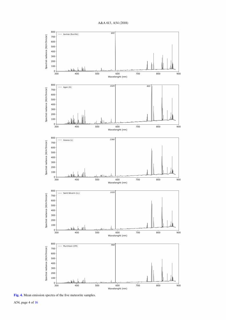
The general layout of the facility is presented in Fig. 2. Botha camera and a spectrograph, which were both operating in thevisible wavelength range, were placed outside the chamber andcontinuously recorded images (e.g., Fig. 3) and emission spectra(Fig. 4), respectively, during the experiments. The video acqui-sition had a frame rate of 10 kHz. The spectroscopic data wereacquired with an Echelle spectrograph (Aryelle 150 of LTB) overthe 250–880 nm wavelength range with an average spectral res-olution of ∼0.08 nm pix−1 (Loehle et al. 2017) and a frequencyof ∼10 spectra per second. Several tens to a few hundreds spec-tra were recorded for each sample during the experiments. Forthe spectral analysis, we only considered the spectra that werecollected during the peak of the emission (which lasted ∼2 s)that we averaged (average of about 20 spectra per sample) toproduce one mean spectrum per sample. The mean spectra ofeach sample/experiment are presented in Fig. 4. The mean spec-tra recorded by Loehle et al. (2017) for the H chondrite EM132,terrestrial argillite, and basalt, respectively, were also used forthe present spectral analysis and are shown in Appendix A.

2.2. Samples

The samples (see Table 1) were selected with the aim of cov-ering as much as possible the meteorite diversity. As a matterof fact, ordinary H, L, and LL chondrites represent ∼75% of

A54, page 2 of 16

A. Drouard et al.: Probing the use of spectroscopy to determine the meteoritic analogues of meteors

Fig. 2. General layout of the facility. Upper panel: the wind tunnel hasseveral windows, so that a variety of instruments can simultaneouslyrecord the experiment that is taking place inside the vacuum chamber.Lower panel: view of the vacuum chamber (open) with an emphasis onthe sample probe, plasma generator and spectrometer is shown.

the falls and more than 97% of anhydrous (EH, EL, H, L, andLL) chondrites, CMs are the most common carbonaceous chon-drites (∼25% of all CCs) and eucrites are the most commontype of achondrites (∼40% of all achondrites). These statisticswere retrieved from the Meteoritical Bulletin Database1. We didnot perform an experiment on an iron meteorite as we expectan emission spectrum only formed by metallic (Fe, Ni) lines.Second, the samples (in particular the H, L, and LL suite) werechosen to probe the ability of spectroscopy to distinguish themeteoritic analogues of meteors. Effectively, the elemental com-position only slightly varies between the three ordinary chondritesubclasses (see Table 2).

3. Spectral analysis

All spectra consist of a thermal continuum (grey body of thesample) on which atomic emission lines (gaseous phase) aresuperimposed. As a first step (Sect. 3.1), we identified all emis-sion lines and compared the occurrence of each element, in termsof number of lines with respect to the total number of lines, with

1 https://www.lpi.usra.edu/meteor/

Fig. 3. Ablation of Juvinas (eucrite). One can clearly observe the strongeffect of the aerothermal heating with the liquid behaviour of the surfaceflowing along the plasma flow and splashing some droplets of mate-rial. In spite of similar experimental conditions and ablation durations(∼2–7 s), measured mass losses are highly variable for the differentsamples. For example, Agen (H) was significantly less ablated (massloss of 0.16 g) than Granes (L; mass loss of 2.89 g).

Table 1. Samples selected for our experiments with their ablationduration (∆t).

Sample name Conservation Clan ∆t

Agen MNHN H 2 sGranes MNHN L 7 sSt-Séverin MNHN LL 3 sMurchison NMNH CM 6 sJuvinas MNHN Eucrite 7 s

Notes. MNHN = Museum National d’Histoire Naturelle, Paris, France.NMNH = National Museum of Natural History, Washington DC, USA.

the bulk composition (Table 2). As a second step (Sect. 3.2),we derived mass ratios for each vapourized sample (Mg/Fe andNa/Fe) using two approaches to be directly compared with itsbulk composition (Table 2).

3.1. Identification and characterization of the emission lines

A first visual inspection of the data reveals an overall spec-tral similarity from one sample to another, and there are twomain groups of lines at short (350–580 nm) and long (700–900 nm) wavelengths, respectively, separated by two very brightsodium lines at 589 nm (see Fig. 4). The only visible differ-ence is the difference in line intensity between the spectra (e.g.the lines of the Agen meteorite are more intense than those ofGranes).

As a next step, we identified for all spectra the atomicelement associated with each emission line using the NISTdatabase2 as well as the total number of lines per element. Anexample of the line identification step is highlighted for the Hchondrite EM132 in Appendix A where 304 lines were identi-fied (a non-exhaustive list of lines is presented in Appendix B).First of all, it appears that all the identified lines are neutral,

2 https://www.nist.gov/pml/atomic-spectra-database

A54, page 3 of 16

A&A 613, A54 (2018)

Fig. 4. Mean emission spectra of the five meteorite samples.

A54, page 4 of 16

A. Drouard et al.: Probing the use of spectroscopy to determine the meteoritic analogues of meteors

Table 2. Mean bulk chemical composition (weight %) of the variousmeteorite classes.

H L LL CM HED Argilite Basalt

Si 16.9 18.5 19.0 13.3 23.0 14.66 20.17Ti 0.060 0.063 0.069 0.069 0.35 0.27 1.52Al 1.13 1.22 1.10 1.12 6.93 5.95 6.85Cr 0.366 0.388 0.41 0.303 0.22 0.0052 0.043Fe 27.5 21.5 19.1 20.6 14.3 2.66 8.74Mn 0.232 0.257 0.22 0.160 0.43 0.041 0.16Mg 14.0 14.9 15.2 11.9 4.15 2.45 6.66Ca 1.25 1.31 1.40 1.29 7.43 15.57 7.02Na 0.64 0.70 0.73 0.30 0.30 0.096 2.88K 0.078 0.083 0.091 0.029 0.025 1.59 1.44P 0.108 0.095 0.103 0.100 – – 0.39Ni 1.60 1.20 0.89 1.20 – 0.0024 0.0026Co 0.081 0.059 0.040 0.058 – 0.00087 0.0048S 2.0 2.2 3.4 2.3 0.07 – –H2O – – – 12.6 – – –C 0.11 0.09 0.022 1.88 – – –O 35.7 37.7 38.275 43.2 43.2 31.0 42.8

Notes. For Murchison (CM) and Saint-Séverin (LL), the bulk compo-sition was retrieved from the literature (Jarosewich 1990). For the H,L, and eucrite meteoritic samples, we used the mean bulk compositionof the respective classes from Hutchison (2004). We also add the bulkcomposition (weight %) of terrestrial argillite and basalt, measured atthe French institute SARM using mass spectrometry. Spectra for the lat-ter two samples were presented in Loehle et al. (2017) but analysed inthe present paper. SARM = Service d’Analyse des Roches et Minéraux,Strasbourg, France.

that is no ionized lines are present in our spectra. Second,it appears that the first group of lines (350–580 nm range)comprises only elements that originate from the sample itself[iron (Fe), magnesium (Mg), manganese (Mn), calcium (Ca),sodium (Na), chromium (Cr), potassium (K), hydrogen (H)],whereas the second group of lines (700–900 nm range) com-prises the atomic lines of the plasma radiation [nitrogen (N)lines]. The few oxygen (O) lines in the second group canbe attributed to the sample and the plasma but in unknownproportion.

In Fig. 5 we show for the H chondrite EM132 the fre-quency of occurrence of lines for each element that we comparewith the average bulk composition (weight %) of H chondrites(Hutchison 2004). It appears that the discrepancy between thetwo histograms is significant. Three of the four most abun-dant elements in H chondrites (O, Si, Mg) are either missing(Si) or are under-represented (O, Mg). On the other hand,Fe is significantly over-represented (iron lines represent 75%of all lines). It thus appears that for a given meteorite, thefrequency of occurrence of lines for each element does notreflect the sample composition. This result is not surprisingand simply reflects the number of emission lines per atomand is in perfect agreement with the spectral lines listed foreach element in the NIST database; Fe lines largely dominatethe list.

We obtained similar results for the other meteorite classesexcept for the eucrite Juvinas whose spectrum is depleted inNi lines, in agreement with the Ni-free composition of eucritesand achondrites in general Jarosewich (1990). In the case ofthe two terrestrial samples (argillite and basalt), there are no Fe

Fig. 5. Upper panel: spectral line distribution per element (%). Lowerpanel: mean bulk composition is shown. The values plotted here comefrom the EM132 spectrum (H chondrite).

and Ni emission lines. This, as in the eucrite case, is in perfectagreement with their Fe- and Ni-free bulk composition.

We investigated, as a next step, whether the absolute intensityof the emission lines, without considering the emission coeffi-cient, for different atoms (Na, Mg, Fe, Ni, and Cr) could reflectto some extent their intrinsic abundance. It appears that it is notthe case. The two Na emission lines are by far the brightest inall spectra whereas Na is only a minor component (in weight %)of our samples. The same applies for Cr to a lesser extent. Itthus appears that line intensities do not reflect the abundance (inweight %) of a given element.

3.2. Abundance ratio trends

We used the opportunity that the spectra of the various mete-orite classes were obtained in similar experimental conditionsto compare the trend in mass ratio derived from the spectrato that expected from their mean bulk composition. Specifi-cally, we followed two approaches. Concerning the first case,we tested whether line intensities are directly proportional tothe abundance (Nagasawa 1978). The second approach consistedin modelling the spectral lines following the auto-absorptionmodel by Borovicka (1993) whose output gives the abundanceof each element. For the two approaches, we focussed on the fol-lowing relative abundances (Mg/Fe, Na/Fe) because Mg and Feare among the most abundant elements in the considered mete-orites and because Na, although a minor component, is by far theelement with the brightest lines.

3.2.1. Intensity ratios: pure emission

For all spectra, we computed two intensity ratios (Mg/Fe andNa/Fe) using the brightest lines for each element (Fe: 438.35nm; Mg: 518.36 nm; and Na: 589.00 nm) and compared thetrend to that of their mean bulk composition. Such an approachis valid in the case of pure emission Nagasawa (1978), because

A54, page 5 of 16

A&A 613, A54 (2018)

Fig. 6. Intensity ratios weighted by the atomic masses and comparedto the mass ratios derived from the mean bulk densities (deep purple inboth plots). Upper panel: Mg/Fe is shown. Lower panel: Na/Fe is shown.For argillite, no iron was observed so the ratio was not computed.

in that case the intensity of a given line is proportional to theatomic abundance of the emitting element (see Appendix B formore details). The results are shown in Fig. 6. It appears thatthe compositional trend from one meteorite to the other is rarelyrespected (especially in the case of Mg/Fe; see for example Hversus LL). It thus appears that intensity ratios are not informa-tive of the relative abundance (weight %) of given atomic speciesand cannot be used to determine the meteoritic analogue. Thismay stem from the fact that we neglect the auto-absorption ofthe gas and its temperature. A more sophisticated model, suchas that presented in the next section may thus improve thoseresults.

3.2.2. Spectral modelling: Autoabsorption model

Our method is based on the auto-absorption model by Borovicka(1993) and has only two free parameters, namely the gas temper-ature and the column density (see Appendix B for a descriptionof the model). Both variables were constrained by minimizingthe difference between the integrated area under the spectral lineand model. Specifically, we first constrained the temperature ofthe gas by applying the model to the iron lines. This allowed usto derive a gas temperature of about 4000 K. Such mean temper-ature value was obtained by best-fitting the iron lines assuminga similar column density. We then applied the model to other

Table 3. Atomic column densities derived from the output column den-sities for sodium (line at 589.00 nm), magnesium (line at 518.36 nm)and iron (line at 438.35, 526.95, and 532.80 nm).

Sample NNa NFe NMg(1015cm−2) (1015cm−2) (1015cm−2)

Agen 6.02 484.0 3.99Argilitte 0.22 – –Basalt 3.79 0.31 –EM132 1.90 4.84 1.59Granes 19.0 15.3 1.59Juvinas 1.35 2.42 0.16Murchison 3.80 9.66 1.12St-Séverin 6.02 9.66 1.12

spectral lines with a fixed temperature of 4000 K to constrain thecolumn densities of each element; we made this assumption ofapplying the model to all the spectral lines because the exper-imental conditions were the same for all samples. The derivedcolumn densities are presented in Table 3. We also derived thesurface temperature of each sample by fitting the thermal contin-uum of its spectrum with a Planck function (emissivity of 0.83following Loehle et al. 2017). It appears that all surface tem-peratures fall in the 2100–2500 K range. Finally, we derived theMg/Fe and Na/Fe mass ratios for all samples and compared themwith those expected from their mean bulk composition (Fig. 7).

Concerning the derived Mg/Fe and Na/Fe mass ratios, weobserved – similar to the previous subsection – a significantdiscrepancy between the inferred and expected mass ratios (afactor of 10 or more). We also observed that for a similar bulkcompositions (H, L, and LL chondrites), the compositional trend(increasing Mg/Fe ratios from H to LL) is not retrieved with theL chondrite Granes having the highest mass ratio. Importantly,the two experiments for H chondrites (EM132 and Agen) high-light that the derived uncertainty (with our model) for the Mg/Feand Na/Fe mass ratios for a given meteorite class is comparableto the expected difference between different meteorite classes(e.g. between H and CM chondrites). Our results thereforeimply that there is no straightforward link between the bulkcomposition of a sample and the spectrum resulting from itsablation.

4. Discussion

We performed ablation experiments in a wind tunnel of five dif-ferent meteorite types (H, L, LL, CM, and eucrite) with thespecific aim to determine whether spectroscopy can be a use-ful tool for determining the meteoritic analogue of meteors.A spectral analysis of the obtained spectra reveals a number ofdifficulties that we summarize hereafter:(i) Silicon (Si) is one of the four major atomic elements (in

weight %) present in all five meteorites. Yet, the emissionlines associated with this element are absent from all spectra.

(ii) Volatiles (e.g. Na) are overestimated with respect to otherelements (e.g. Fe or Mg) even though these are minorcomponents.

(iii) Mass ratios (Mg/Fe and Na/Fe) derived under differentassumptions (pure emission and auto-absorption model) donot reflect the true composition of the samples nor relativedifferences in composition.Case (i) may be because the temperatures reached during the

experiments (∼4000 K) were too low to dissociate the very stable

A54, page 6 of 16

A. Drouard et al.: Probing the use of spectroscopy to determine the meteoritic analogues of meteors

Fig. 7. Mass ratios derived from the model compared to the averagecomposition of the sample. For argillite, no iron was observed so ratioswere not computed. Upper panel: derived Mg/Fe (light purple) andexpected one (deep purple). Lower panel: derived Na/Fe (light purple)and expected one (deep purple).

gaseous SiO molecule resulting from the ablation of the solidSiO2 phase and that there were likely no free Si atoms in thegas. Such low experimental temperatures may also explain whyall emission lines observed in our spectra are neutral lines. Incontrast, meteor spectra reveal the presence of numerous ionizedlines (so-called second component at 10 000 K; see Borovicka1993), which can be explained by the higher entry velocities(∼20–70 km s−1) of bolides with respect to those we simulated inour experiments (∼10 km s−1). Table 4 illustrates this point wellby showing the energy required for ionization for each element.

Case (ii) can be explained, at first order, as the byproductof two physical quantities, namely the melting and vapouriza-tion temperature of a given element (Table 4). Sodium (Na) andpotassium (K) illustrate this case particularly well. First, theirfavourably high emission coefficient implies that the intrinsicintensity of their emission line is higher than that of other ele-ments with lower emission coefficients. Second, their low fusionand vapourization temperature implies that the gas gets enrichedsignificantly more in those two elements than in others such asiron. As a matter of fact, the high temporal spectra resolution ofour measurements allowed us to observe the rapid apparition ofvolatiles such as sodium with respect to metallic elements such

Table 4. Some physical data of the main important elements of mete-orites compositions.

Sublimation Fusion Vaporization 1st ionizationenthalpy temperature temperature potential

(kJ mol−1) (K) (K) (eV)

H 218.00 – – 13.6C 716.68 – 4100 11.3N 472.68 – – 14.5O 249.18 – – 13.6Na 107.30 – 1171 5.1Mg 147.10 923 1366 7.6Al 329.70 933 2791 6.0Si 450.00 1685 3505 8.2K 89.00 336 1040 4.3Ca 177.8 1115 1774 6.1Cr 397.48 2130 2952 6.8Mn 283.26 1519 2235 7.4Fe 415.47 1809 3133 7.9

Notes. Data from the NIST database. Thermodynamical parame-ter: http://webbook.nist.gov/chemistry/form-ser/ and ion-ization potentials: https://www.nist.gov/pml/atomic-spectra-database.

as Fe that appeared later. The temporal shift (about 0.5 s) remainssmall compared to the duration of the emission peak (about 2 s).

Case (iii) is a direct implication of (ii). This is particularlytrue for the first case (pure emission) but should be less true whenusing the model as the latter takes into account the absorptioncoefficient. An obvious caveat of the model is that most elementspossess only a few emission lines (e.g. Mg) limiting the abilityto have a statistical approach in our analysis. In this respect, onlyiron and nickel possess enough emission lines (see Fig. 5).

In summary, the difference in terms of thermodynamicalbehaviour among the elements leads to a spectral variabilityamong different samples (in terms of intensity of the emissionlines) that is very difficult to decode. Such spectral differencecan even be observed in the case of samples with nearly identicalcompositions (see the different values for the two H chondrites;e.g. Figs. 6 and 7).

The line identification step however reveals that spectroscopyis able to distinguish samples that are not made of the sameelements/atoms. For example, there is no nickel in eucrites andthis is well verified via our experiments that show an absence ofnickel lines in the Juvinas spectrum. Similarly, we can identifyterrestrial samples (argillite and basalt) via the absence of ironand nickel emission lines in their spectra. This has global impli-cation for establishing the ability of spectroscopy to determinethe meteoritic analogues of meteors. Whereas all chondrites aremade of the same atoms, the same is not true for achondritesand iron meteorites. The latter are made of Fe, Ni, and Comainly with traces of Ga, Ge and Ir (Jarosewich 1990), whereasthe former do not have any nickel but do have most elementsseen in chondrites (see Table 2). As such, a spectral analysisconsisting of a simple line identification should allow distin-guishing between chondrites, achondrites, and iron meteorites.For this to be the case, the spectral resolution should be suffi-cient to distinguish the individual atomic lines (∼0.1 nm pix−1).We would like to stress that our findings are fully consistent withthe review by Borovicka et al. (2015) in which they propose that

A54, page 7 of 16

A&A 613, A54 (2018)

meteor spectroscopy can be used to distinguish the main types ofincoming meteoroids (chondritic, achondritic, and metallic).

5. Conclusions

Several camera networks have been installed around the worldand have been witnessing the atmospheric entry of severalbolides each year. From those datasets, the orbits of the bolidesare derived along with the distribution ellipse (location of thefall). However, the vast majority of the bolides yield meteoritesin areas unfavourable for their recovery, or are not found onthe ground. For those events, although we have a precise orbitdetermination, we are unfortunately not able to associate a givenmeteorite group with the orbit. Our objective in this work wasto test whether spectroscopy in the visible wavelength range ofthese bolides could allow us to classify the incoming meteoriticmaterial. To test this hypothesis, we performed ablation experi-ments in a wind tunnel on five meteorite types (H, L, LL, CM,and eucrite) simulating the atmospheric entry conditions of ameteoroid at 80 km of altitude for an entry speed of 10 km s−1.Visible spectra with a resolution of ∼0.1 nm pix−1 were collectedduring the entire ablation sequence allowing us to measure thecomposition of the vapourized material.

A detailed spectral analysis including a systematic line iden-tification and mass ratio determinations (Mg/Fe, Na/Fe) withor without a spectral model was subsequently performed on allspectra. It appears that spectroscopy, via a simple line identifica-tion, can allow us to distinguish the three main meteorite classes(chondrites, achondrites, and irons), but it has not the potential todistinguish for example an H chondrite from a CM chondrite. Italso appears that mass ratios are not informative about the natureof the vapourized material.

Regarding the future of meteor spectroscopy, distinguishingthe three main classes of meteorites (chondrites, achondrites,and irons), in particular the fraction of iron-like bolides could bean interesting project as it could help quantify the amplitude ofthe atmospheric bias with respect to meteorite fall statistics. Toinvestigate such question, spectroscopy in the 400–600 nm wave-length range with a resolution of 0.1 nm pix−1 would be ideal as itwould allow us to resolve the emission lines of the key elements(Fe, Ni, Mg, Cr, Na, and Si).

To conclude, the source location within the main belt ofthe different meteorite classes (H, L, LL, CM, CI, etc.) shouldcontinue to be investigated via fireball observation networks.Spectroscopy of incoming bolides will only marginally help clas-sify the incoming material precisely (iron meteorites only). Toreach a statistically significant sample of recovered meteoritesalong with accurate orbits (>100) within a reasonable time frame(10–20 years), the optimal solution maybe to extend spatiallyexisting fireball observation networks.

Acknowledgements. We thank the Programme National de Planétologie, the Lab-oratoire d’Astrophysique de Marseille and the Agence Nationale de la Recherche(FRIPON project: ANR-13-BS05-0009) for providing financial support for theseexperiments.

ReferencesBabadzhanov, P. B., & Kokhirova, G. I. 2004, A&A, 424, 317Binzel, R. P., & Xu, S. 1993, Science, 260, 186Bland, P. A., Towner, M. C., Paxman, J. P., et al. 2014, in LPI Contributions, 77th

Annual Meeting of the Meteoritical Society, 1800, 5287Bloxam, K., & Campbell-Brown, M. 2017, Planet. Space Sci., 143, 28Borovicka, J. 1993, A&A, 279, 627Borovicka, J. 1994, Meteoritics, 29, 446Borovicka, J. 2005, Earth Moon and Planets, 97, 279

Borovicka, J., Spurný, P., Kalenda, P., & Tagliaferri, E. 2003, Meteor. Planet.Sci., 38, 975

Borovicka, J., Koten, P., Spurný, P., Bocek, J., & Štork R. 2005, Icarus, 174, 15Borovicka, J., Spurný, P., Brown, P., et al. 2013a, Nature, 503, 235Borovicka, J., Tóth, J., Igaz, A., et al. 2013b, Meteor. Planet. Sci., 48, 1757Borovicka, J., Spurný, P., & Brown, P. 2015, Small Near-Earth Asteroids as a

Source of Meteorites, eds. P. Michel, F. E. DeMeo, & W. F. Bottke, 257Boyd, I. D. 2000, Earth Moon and Planets, 82, 93Brown, P., Ceplecha, Z., Hawkes, R. L., et al. 1994, Nature, 367, 624Brown, P. G., Hildebrand, A. R., Zolensky, M. E., et al. 2000, Science, 290, 320Brown, P., Jones, J., Weryk, R. J., & Campbell-Brown, M. D. 2004, Earth Moon

and Planets, 95, 617Brown, P., McCausland, P. J. A., Fries, M., et al. 2011, Meteor. Planet. Sci., 46, 339Ceplecha, Z. 1960, Bull. Astron. Inst. Czechoslov., 11, 164Cevolani, G., Pupillo, G., Bortolotti, G., et al. 2008, Mem. S.A.It. Suppl., 12, 39Colas, F., Zanda, B., Bouley, S., et al. 2015, European 80 Planetary Sci-

ence Congress 2015, Online at: http://meetingorganizer.copernicus.org/EPSC2015/EPSC2015

Dyl, K. A., Benedix, G. K., Bland, P. A., et al. 2016, Meteor. Planet. Sci., 51,596

Friichtenicht, J. F., Slattery, J. C., & Tagliaferri, E. 1968, ApJ, 151, 747Gardiol, D., Cellino, A., & Di Martino M. 2016, in International Meteor

Conference Egmond, eds. A. Roggemans & P. Roggemans, 76Haack, H., Michelsen, R., Stober, G., Keuer, D., & Singer, W. 2010, Meteorit.

Planet. Sci. Suppl., 73, 5085Halliday, I., Griffin, A. A., & Blackwell, A. T. 1981, Meteoritics, 16, 153Hildebrand, A. R., Milley, E. P., Brown, P. G., et al. 2009, in Lunar and Planetary

Science Conference, 40, 2505Hutchison, R. 2004, Meteorites: a Petrologic, Chemical and Isotopic Synthesis

(Cambridge: Cambridge Univ. Press)Hutchison, R., Williams, I. P., & Russell, S. S. 2001, Phil. Trans. R. Soc. Lond.,

Ser. A, 359, 2077Jarosewich, E. 1990, Meteoritics, 25, 323Jenniskens, P., Vaubaillon, J., Binzel, R. P., et al. 2010, Meteor. Planet. Sci., 45,

1590Jenniskens, P., Fries, M. D., Yin, Q.-Z., et al. 2012, Science, 338, 1583Kasuga, T., Watanabe, J., Ebizuka, N., Sugaya, T., & Sato, Y. 2004, A&A, 424,

L35Koukal, J., Srba, J., Gorková, S., et al. 2016, in International Meteor Conference

Egmond, eds. A. Roggemans & P. Roggemans, 137Loehle, S., Zander, F., Hermann, T., et al. 2017, ApJ, 837, 112Madiedo, J. M., & Trigo-Rodriguez, J. M. 2014, Meteoroids 2013Madiedo, J. M., Trigo-Rodríguez, J. M., Castro-Tirado, A. J., Ortiz, J. L., &

Cabrera-Ca no J. 2013, MNRAS, 436, 2818Madiedo, J. M., Trigo-Rodríguez, J. M., Zamorano, J., et al. 2014, A&A, 569,

A104McCrosky, R. E., Posen, A., Schwartz, G., & Shao, C.-Y. 1971, J. Geophys. Res.,

76, 4090McSween, H. Y., Binzel, R. P., de Sanctis, M. C., et al. 2013, Meteor. Planet. Sci.,

48, 2090Milley, E. P., Hawkes, R. L., & Ehrman, J. M. 2007, MNRAS, 382, L67Mozgova, A. M., Borovicka, J., Spurny, P., & Churyumov, K. I. 2015, Odessa

Astronomical Publications, 28, 289Nagasawa, K. 1978, Annals of the Tokyo Astronomical Observatory, 16, 157Shepard, C. E., Vorreiter, J. W., Stine, H. A., & Winovich, W. 1967, A Study of

Artificial Meteors as Ablators, Tech. rep., NASA TN D–3740 (Moffett Field,CA: NASA Ames Research Center)

Simon, S. B., Grossman, L., Clayton, R. N., et al. 2004, Meteor. Planet. Sci., 39,625

Spurný, P., Oberst, J., & Heinlein, D. 2003, Nature, 423, 151Spurný, P., Borovicka, J., Kac, J., et al. 2010, Meteor. Planet. Sci., 45, 1392Spurný, P., Bland, P. A., Shrbený, L., et al. 2012a, Meteor. Planet. Sci., 47, 163Spurný, P., Haloda, J., & Borovicka, J. 2012b, in LPI Contributions, Asteroids,

Comets, Meteors 2012, 6143Trigo-Rodríguez, J. M., Llorca, J., Borovicka, J., & Fabregat, J. 2003, Meteor.

Planet. Sci., 38, 1283Trigo-Rodríguez, J. M., Llorca, J., Borovicka, J., & Fabregat, J. 2004a, Earth

Moon and Planets, 95, 375Trigo-Rodríguez, J. M., Llorca, J., & Fabregat, J. 2004b, MNRAS, 348, 802Trigo-Rodriguez, J. M., Llorca, J., Ortiz, J. L., et al. 2004c, Meteor. Planet. Sci.

Supp., 39Vernazza, P., Binzel, R. P., Thomas, C. A., et al. 2008, Nature, 454, 858Vernazza, P., Zanda, B., Binzel, R. P., et al. 2014, ApJ, 791, 120Vernazza, P., Marsset, M., Beck, P., et al. 2016, AJ, 152, 54Vojácek, V., Borovicka, J., Koten, P., Spurný, P., & Štork R. 2015, A&A, 580,

A67

A54, page 8 of 16

A. Drouard et al.: Probing the use of spectroscopy to determine the meteoritic analogues of meteors

Appendix A: Additional figures

Fig. A.1. Identification of the emission lines of the EM132 spectrum (H chondrite) using the NIST database (shift <0.1 nm).

A54, page 9 of 16

A&A 613, A54 (2018)

Fig. A.1. continued

A54, page 10 of 16

A. Drouard et al.: Probing the use of spectroscopy to determine the meteoritic analogues of meteors

Fig. A.1. continued

A54, page 11 of 16

A&A 613, A54 (2018)

Fig. A.1. continued

A54, page 12 of 16

A. Drouard et al.: Probing the use of spectroscopy to determine the meteoritic analogues of meteors

Fig. A.2. Spectra collected by Loehle et al. (2017) for the H chondrite EM132 and two terrestrial analogues (argillite, basalt).

A54, page 13 of 16

A&A 613, A54 (2018)

Appendix B: Methods of spectral modelling

Here we present in detail the two methods we used to deter-mine mass ratios from the spectral lines. We considered first apure emission case in which the emission line intensity is pro-portional to the abundance as presented in Nagasawa (1978) andthen we followed an auto-absorbant gas modelling inspired bythe model presented in Borovicka (1993). The former consid-ers the gas optically thin whereas the latter considers it opticallythick. The first part of this appendix presents the theoreticalscheme of radiative transfer and the limit case to model the emis-sion line intensities. The second and third subsections focus onthe calculation methods for the two cases (pure emission andauto-absorbant gas model).

B.1. Elements of radiative transfer

When modelling the ablation process of our meteorite samples,there are three physical processes that need to be taken intoaccount, namely the thermal emission of the sample, the gasemission of the surrounding gas cloud (air enriched in samplecompounds by its partial vapourization), and the absorbant effectof the gas with respect to the above emission lines. We detaileach of these processes hereafter.

We first assume that the thermal emission of the sampleheated by the air friction follows the Planck distribution. Theblack-body emission at a temperature T is frequency dependentand can be written as

Bν(T ) =2hν3

c2

1ehν/kBT − 1

(B.1)

where ν is the frequency, c the light celerity, h the Planck con-stant and kB the Boltzmann constant. The samples were assumedto be grey bodies, implying that their thermal emission Isolid

ν isa fraction of the Planck function. The emissivity was set at 0.83for our experimental conditions (Loehle et al. 2017).

As a next step, we modelled the theoretical emission of thehot gas resulting from the sample ablation assuming that(i) The gas is in thermal equilibrium. This classical assumption

allows the atomic population derivation and is supported bysome theoretical approaches (Boyd 2000).

(ii) The gas is auto-absorbent without diffusion. Following theresults of Borovicka (1993), we model the gas emissionincluding the auto-absorption.

(iii) The line profiles are Voigt profiles. A Voigt profile consistsof the convolution of a Gaussian profile and a Lorentzianprofile. It represents well the two main physical processesinvolved in the line enlargement, i.e. the Doppler enlarge-ment and the natural enlargement, respectively.

(iv) The same profile in emission and absorption. It impliesthat the profiles of absorption, spontaneous emission andstimulated emission are the same.

(v) The line spread function has a gaussian shape. The instru-mental response consists of the convolution of the modelledintensity with a Gaussian function.In this framework, the gas can be described by the coeffi-

cients εν and κν, which are the emission and absorption coef-ficients of the gas, respectively. Depending on the frequencyν, assuming (i) and (iv), these coefficients can be written asfollows:

εν =hν4π

Aul nu Φ(ν) (B.2)

κν =c2

8πν2 Aul nlgu

gl(1 − e−hν/kBTgas ) Φ(ν) (B.3)

where h is the Planck constant, kB the Boltzmann constant andthe following notation:

Aul Einstein coefficient of spontaneous emissionnu upper level populationnl lower level populationgu upper level statistic weightgl lower level statistic weightφ(ν) line profile

The emission and absorption coefficients are related to theline profile, assumed to be a Voigt profile (iii),

φν =

∫ +∞

−∞

1π∆νD

e−(ν′−νul∆νD

)2

∗δ

δ2 + (ν − ν′)2 dν′ = H(∆νD,Γ)

(B.4)

where ∆νD is the Doppler width and δ the lorentzian parameter,defined as follows:

∆νD =νul

c

√2kBTgas

mδ =

14π

∑l<u

Aul =Γ

4π(B.5)

where m is the atomic mass of the studied element and Γ thedamping constant.

In order to write the radiative transfer equation, we firstderived the source function S ν, ratio of the emission to theabsorption coefficient. The source function is, following ourassumptions, only temperature dependent because it can bewritten as a Planck function,

S ν =ενκν

= Bν(Tgas) (B.6)

Let Iν be the spectral radiance measured by the spectrometerat a given frequency ν. Let τν be the optical thickness definedfrom the sample (see Fig. B.1). The optical thickness is definedby τν = κν L, where L the thickness of the emitting cloud alongthe line of sight and κν the absorption coefficient. The energyconservation can be written in terms of local variations of thespectral radiance at a given frequency with respect to the opti-cal depth, leading to the following general equation of radiativetransfer in a medium without diffusion:

dIνdτν

= S ν − Iν (B.7)

The general solution can be written as

Iν(τν) = Iν(τν = 0) e−τν +

∫ τν

0S ν(τ′ν) eτν−τ

′ν dτ′ν (B.8)

Following previous assumptions, Iν(τν = 0) = Isampleν . More-

over, because the source function is temperature dependent only,it is uniform for the optical thickness and:

Iν(τν) = Isolidν e−τν + Bν(Tgas)(1 − e−τν ) (B.9)

As expected, the spectral radiance measured in the spec-trometer is the addition of the thermal continuum of the sam-ple and the spectral lines of the hot surrounding gas cloud.The intensity collected in the spectrometer is simply Iν(τmax

ν ),

A54, page 14 of 16

A. Drouard et al.: Probing the use of spectroscopy to determine the meteoritic analogues of meteors

Table B.1. Main lines for each element with their spontaneous emissioncoefficient and the upper level degeneracy.

Element λ Aul gu

Fe I 381.58 1.12 × 108 7382.78 1.05 × 108 5404.58 8.62 × 107 9438.35 5.00 × 107 11440.48 2.75 × 107 9441.51 1.19 × 107 7

Ni I 349.30 9.80 × 107 3547.69 9.50 × 106 3

Mn I 403.08 1.70 × 107 8403.31 1.65 × 107 6403.45 1.58 × 107 4

K I 766.49 3.80 × 107 4769.90 3.75 × 107 2

Cr I 425.44 3.15 × 107 9427.48 3.07 × 107 7428.97 3.16 × 107 5520.45 5.09 × 107 3520.60 5.14 × 107 5520.84 5.06 × 107 7

Mg I 516.73 1.13 × 107 3517.27 3.37 × 107 3518.36 5.61 × 107 3

Na I 589.00 6.16 × 107 4589.60 6.14 × 107 2

Fig. B.1. Origin and axis definitions of the optical thickness. τmaxν is

defined as the total optical thickness of the cloud.

defined in Fig. B.1, where τmaxν = κνL, L is the cloud radius. The

optical thickness was set at L = 30.0 cm, a reasonable distanceconsidering the dimensions of the facilities.

We finally can write the spectral line intensity Ithinν (τν)

and Ithickν (τν) for a gas optically thin (Sect. 3.2.1) or thick

(Sect. 3.2.2), respectively, as

Ithinν (τν) = lim

τν→0Iν(τν) =

hν4π

Aul nu L Φ(ν) (B.10)

Ithickν (τν) = Isample

ν e−τν + Bν(Tgas)(1 − e−τν ) (B.11)

B.2. Optically thin case

In such a case, the integrated intensity along the considered spec-tral line is proportional to the upper level population following

Fig. B.2. Sodium line (589.0 nm) of the sample EM132 plotted with itsmodelled line (outputs: T = 3200 K and n = 9.8 × 1014).

Eq. (B.10) and therefore to the atomic population in the gas usingthe Boltzmann distribution

nu = ngu

Ue−Φu/kBT (B.12)

This implies a proportionality between intensity ratios and massratios. We can therefore compare intensity ratios between vari-ous spectra using the same spectral lines. In the present study,we derived two intensity ratios (Mg/Fe, Na/Fe) that we weightedby the atomic masses. For example, in the case of Mg/Fe, theprocedure is as follows:

rMg/Fe =IMgmMg

IFemFe (B.13)

B.3. Optically thick case

Considering an optically thick case, the intensity is described byEq. (B.11) and has to be integrated numerically. We remind herethat the area under an emission line depends only on two freeparameters, namely the temperature and atomic abundance inthe lower level (see first section). To derive both parameters, weminimized the integrated intensity difference between the exper-imental data and the model points using the least-squares fittingmethod (Fig. B.2). We applied this fitting technique to severaliron emission lines and determined the gas temperature in thisway. We then kept this temperature fixed and ran the model onthe lines of interest (Na, Mg, and Fe) to determine the atomicabundance of these species in the lower level.

In order to perform the least-squares method with thedata, we convolved the computed intensity Iν(τmax

ν ) with theinstrumental response (a Gaussian following (v). The syntheticspectral line intensity (Isynth

ν ) is therefore expressed as:

Isynthν =

∫ +∞

−∞

Iν(τmaxν ) ∗ e−

(ν′−νul

2σ

)2

dν′ (B.14)

where σ is the full width at half-maximum and corresponds tothe spectral distance between two pixels.

As a next step, we constrained for each element (Na, Mg,and Fe) the total atomic population present in the gas using theBoltzmann distribution that allows us to link the lower level pop-ulation nl to the atomic population n via the following relation:

nl = ngl

Ue−Φl/kBT (B.15)

A54, page 15 of 16

A&A 613, A54 (2018)

Finally, we derived the mass ratios (Mg/Fe, Na/Fe) using thepreviously estimated atomic populations that we weighted by theatomic mass. For example, in the case of Mg/Fe, the procedureis as follows:

rMg/Fe =nMgmMg

nFemFe (B.16)

Appendix C: Additional tables

Table C.1. Mg/Fe.

Sample Mean bulk Intensity ratio Spectral modelling

Agen 0.51 0.078 ± 0.01 0.004 ± 0.002Argilitte 0.92 – –Basalt 0.76 – –EM132 0.51 0.11 ± 0.01 0.14 ± 0.01Granes 0.69 0.08 ± 0.01 0.045 ± 0.008Juvinas 0.29 0.04 ± 0.01 0.028 ± 0.008Murchison 0.58 0.07 ± 0.01 0.051 ± 0.008St-Séverin 0.80 0.07 ± 0.01 0.051 ± 0.008

Table C.2. Na/Fe.

Sample Mean bulk Intensity ratio Spectral modelling

Agen 0.023 1.3 ± 0.2 0.01 ± 0.09Argilitte 0.036 – –Basalt 0.33 24.3 ± 0.6 5.1 ± 0.06EM132 0.023 2.9 ± 0.2 0.16 ± 0.07Granes 0.033 8.1 ± 0.3 0.51 ± 0.08Juvinas 0.021 3.8 ± 0.1 0.20 ± 0.07Murchison 0.020 3.6 ± 0.1 0.16 ± 0.07St-Séverin 0.038 4.1 ± 0.2 0.26 ± 0.07

A54, page 16 of 16