PROBABILITY THEORY NOTES

1/10/07

Definition 1. An elementary experiment or Bernoulli trial is an experiment with two outcomes: 1 and 0.Here, 1 will often be thought of as success or as heads and 0 will be thought of as failure or tails.

Definition 2. A sequence of n elementary experiments (for a fixed n) is called a composite experiment. Inother words, this is just a sequence of 1’s and 0’s.

Definition 3. The set of all outcomes of a composite experiment is denoted Ωn = 0, 1n and is called thesample space.

Define a function Pn : P (Ωn) −→ [0, 1], where if ω ∈ Ωn and ω = (ω1, . . . , ωn), thne Pn (ωi = 0) = qand Pn (ωi = 1) = p with p + q = 1. We will assume the independence assumption, which is that for(e1, . . . , ei) ∈ 0, 1i, then

Pn [ωi+1 = 1 and (ω1, . . . , ωi) = (e1, . . . , ei)] = Pn [ωi+1 = 1] · Pn [(ω1, . . . , ωi) = (e1, . . . , ei)] .

Thus, if E ⊂ Ωn, then Pn [E] =∑

ω∈E Pn [ω]. This last property is called the additive property.We see that the σ-algebra on Ωn is P (Ωn) and Pn is a measure on P (Ωn). Also note that Pn(ω) =

pSn(ω) · q1−Sn(ω), where Sn(ω) =∑n

i=1 ωi, which is the number of 1’s in ω. Note also that Sn : Ωn −→ [0, n].We call this Ωn = 0, 1n with product probability (q, p)⊗n.

Proposition 1 (4.1).

Pn(Sn = k) =(

n

k

)pkqn−k

for k ∈ 0, 1, . . . , n.

Proof. By the independence assumption and additivity.

Proposition 2 (4.3). (1) The expected value of Sn is E[Sn] = np.(2) The variance of Sn is Var[Sn] = npq = np(1− p).

Proof. Frist, note that E[Sn] =∑n

k=0 k · Pn [Sn = k] =∑n

k=0 k(nk

)pk(1 − p)k. Notice that (p + q)n =∑n

k=0

(nk

)pkqn−k and d

dp (p + q)n = n(p + q)n−1, which is to say

np = np(p + q)n−1 =n∑

k=0

k

(n

k

)pkqn−k

=n∑

k=0

k

(n

k

)pk(1− p)n−k = E[Sn].

For the second part, note that

E[S2n] =

n∑k=0

k2

(n

k

)pk(1− p)n−k.

If we consider the second derivative (with respect to q) of the binomial theorem, we get

n(n− 1)(p + q)n−2 =n∑

k=0

k(k − 1)(

n

k

)pk−2qn−k,

and since p + q = 1, multiplying by p2 gives us

n(n− 1)p2 =n∑

k=0

k(k − 1)(

n

k

)pkqn−k.

1

Thus, we see that

n(n− 1)p2 + np =n∑

k=0

k2

(n

k

)pkqk = E[S2

n].

Thus, we know that

E[y2]− (E[y])2 = n2p2 − np2 + np− n2p2 = np− np2 = np(1− p).

Remark 1. If y : Ωn −→ R and P is a function on Ωn, then the expectation is E[y] = EP [y] =∫

y dP .This is called the expectation of y or the first moment. Also, E[y2] =

∫y2 dP is the second moment and

Var[y] = E[y2]− E[y]2 = E[(y − E[y])2

]is the variance or the second central moment.

Proposition 3 (4.2). If X1, . . . , Xn are independent Bernoulli trials with parameter p, then their sumSn = X1 + · · ·+ Xn is a binomial random variable with parameters n and p.

Definition 4. Sn is a binomial random variable (binomial r.v.) if P [Sn = k] =(nk

)pk(1− p)k.

Proof. Count all possibilities of k successes for n trials.

Proof. (Number 2 of Proposition 2)For the first one:

E[Sn] = E[X1 + · · ·+ Xn] = E[X1] + · · ·+ E[Xn] = p + · · ·+ p︸ ︷︷ ︸n times

= np.

For the second statement,

Var[Sn] = Var[X1 + · · ·+ Xn] = Var[X1] + · · ·+ Var[Xn] = (p− p2) + · · ·+ (p− p2) = n(p− p2) = np(1− p).

Proposition 4 (Markov’s Inequality,2.1). Suppose X : Ω −→ R≥0. Then

P [X ≥ a] ≤ E[X]a

.

Proof.

P[X ≥ a] =∑xi≥a

P[X = Xi] ≤∑xi≥a

xi

aP[X = Xi] ≤

1a

∑xi

xiP[X = Xi] =E[X]

a.

Proposition 5 (Bienayme-Chebyshev Inequality,2.2).

P [|X − E[X]| ≥ a] ≤ 1a2

Var[X].

Proof.

P [|X − E[X]| ≥ a] = PE[(X − E[X])2 ≥ a2

]≤ 1

a2E[(X − E[X])2

]=

Var[X]a2

.

Theorem 1 (The Weak Law of Large Numbers, 5.1). (Proof and statement in one.)

P [|Sn − np| ≥ nε] ≤ 1n2ε2

Var[Sn] =np(1− p)

n2ε2=

p(1− p)ε2

· 1n≤ 1

4ε2· 1n

.

Thus,P [|Sn − np| ≥ nε] −→

uniformly in p0 as n →∞.

P[∣∣∣∣Sn

n− p

∣∣∣∣ ≥ ε

]−→

uniformly in p0 as n →∞.

P[∣∣∣∣Sn

n− p

∣∣∣∣ ≥ ε

]= O

(1n

)uniformly in p.

2

Another way of saying this is that

limn→∞

uniformly in p

Pn

[∣∣∣∣Sn

n− p

∣∣∣∣ ≥ ε

]= 0.

1/11/07

Theorem 2 (Weierstrass’ Approximation Theorem). Given f(x) continuous on [a, b] and ε > 0, there existsa polynomial g(x) so that maxx∈[a,b] |f(x)− g(x)| < ε.

Remark 2. (1) If P = polynomials in x on [a, b], then P is dense in C[a, b].(2) Bernstein’s proof is constructive, but not effective. An effective method is to use the Fourier-

Chebyshev series.

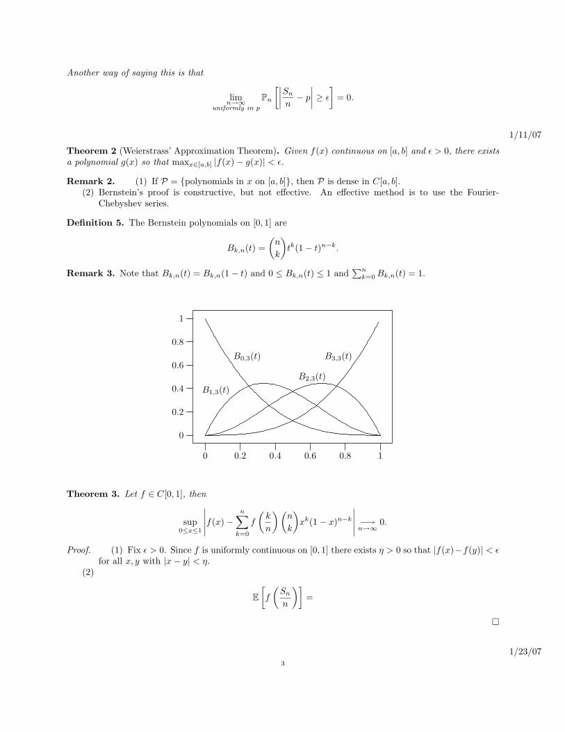
Definition 5. The Bernstein polynomials on [0, 1] are

Bk,n(t) =(

n

k

)tk(1− t)n−k.

Remark 3. Note that Bk,n(t) = Bk,n(1− t) and 0 ≤ Bk,n(t) ≤ 1 and∑n

k=0 Bk,n(t) = 1.

B0,3(t)

B1,3(t)B2,3(t)

B3,3(t)

0 0.2 0.4 0.6 0.8 1

0

0.2

0.4

0.6

0.8

1

Theorem 3. Let f ∈ C[0, 1], then

sup0≤x≤1

∣∣∣∣∣f(x)−n∑

k=0

f

(k

n

)(n

k

)xk(1− x)n−k

∣∣∣∣∣ −→n→∞0.

Proof. (1) Fix ε > 0. Since f is uniformly continuous on [0, 1] there exists η > 0 so that |f(x)−f(y)| < εfor all x, y with |x− y| < η.

(2)

E[f

(Sn

n

)]=

1/23/073

1. Central Limit Theorem (7.1)

The main players in the development are deMoivre, Laplace and Gauss.We’re interested in the fluctuation of Sn around its mean. From the weak law of large numbers, we know

that Pn(|Sn

n − p| > ε) −→ 0. We also know that Pn(|Sn

n − p| > ε) ≤ e−nh+(ε) + e−nh−(ε). Finally, note thatE((np− Sn)2) = np(1− p).

Theorem 4 (Central Limit Theorem). Let a, b ∈ R ∪ ±∞ with a < b. Then

limn→∞

Pn

(a ≤ Sn − np

√n√

p(1− p)≤ b

)=

1√2π

∫ b

a

e−x22 dx

Remark 4. (1) In the proof of the theorem, we’ll use the fact that

1√2π

∫ ∞

−∞e−

x22 dx = 1.

Proof. To see this, set I =∫∞−∞ e−

x22 dx =

∫∞−∞ e−

y2

2 dy. Then we find that

I2 =∫ ∞

−∞

∫ ∞

−∞e−

(x2+y2)2 dx dy

=∫ 2π

0

∫ ∞

0

e−r22 r dr dθ

= 2π.

(2) Set Φ(y) = 1√2π

∫∞y

e−x2/2 dx. Then we see that

1√2π(y + 1)

(e−y2/2 − e−(y+1)2/2) ≤ Φ(y) ≤ 1√2π

e−y2/2

as y →∞. Thus, Φ(y) ∼ 1√2πy

e−y2/2.

Proof. Set erfc(x) := 1− erf(x) = 2√π

∫∞x

e−x2dx.

Φ(y) =1√2π

∫ ∞

y

e−x2/2 dx

=12erfc(

y√2)

=12

(2√π

∫ ∞

y√2

e−x2dx

)

=1√π

∫ ∞

y√2

−2te−t2

−2tdt

=1√π

e−t2

−2t

∣∣∣∣∣∞

y/√

2

−∫ ∞

y/√

2

e−t2

2t2dt

=

1√π

[e−y2/2

2(1/√

2)− h.o.t.

]

=12

[(2√π

e−y2/2

)(1

2(1/√

2)− Γ(3)(

2(1/√

2))3 +

Γ(5)

2!(2(1/

√2))5 − . . .

)]

=1√2π

e−y2/2 − 3√2πy3

e−y2/2 +3√

2πy5e−y2/2 +O(

1y7

).

4

Thus,

limy→∞

Φ(y)1√2πy

e−y2/2∼ lim

y→∞

1√2πy

e−y2/2

1√2πy

e−y2/2−

3√2πy3 e−y2/2

1√2πy

e−y2/2= lim

y→∞1− 3

y2= 1.

(3) The convergence in CLT is uniform in both a and b. Without loss of generality, we fix a = −∞.Then fn(b) −→ f(b) for b > −∞.

Lemma 1. If fn is a sequence of monotone functions fn : R −→ [0, 1] that converges pointwise tof (which is continuous) and f : R −→ R with f(R) ⊇ (0, 1). Then this convergence is uniform.

Proof. Let ε > 0 be given. Without loss of generality, fn is monotone increasing and limx→−∞ fn(x) =0 and limx→∞ fn(x) = 1. This means that limx→−∞ f(x) = 0 and limx→∞ f(x) = 1. As func-tions, there exists x so that for all z ≥ x, |f(z) − 1| < ε. Let N1 ∈ N be so that n ≥ N1

means that |fn(x) − f(x) < ε and so |fn(x) − 1| < 2ε. Since fn is monotone for all z ≥ x,fn(z)− 1| ≤ |fn(x)− 1| < 2ε. Thus, for all z ≥ x and n ≥ N1, we have

|fn(z)− f(z)| ≤ |fn(z)− 1|+ |f(z)− 1| < 3ε.

Similarly, there exists y and N2 so that for all z ≥ y and all n ≥ N2 we have

fn(z)− f(z)| ≤ |fn(z)|+ |f(z)| < 3ε.

Since [y, x] is compact, we have f(t) is uniformly continuous. There exists δ > 0 for cotninuityon [y, x]. Partition [y, x] into R subintervals, each of diameter less than δ. Choose [aj , bj ] with|bj − aj | < r. There exists mj so that for all n ≥ mj , |fn(aj)− f(aj)| < ε. There exists mj so thatfor all n ≥ mj , |fn(bj)− f(bj)| < ε. Choose n ≥ Mj := maxmj , mj and pick z ∈ [aj , bj ]. Note taht

fn(a) ≤ fn(a) ≤ fn(bj) =⇒ f(a)− ε ≤ fn(z) ≤ f(bj) + ε.

Since |f(b)− f(a)| < ε =⇒ f(b)− 2ε ≤ fn(z) ≤ fn(bj) + ε. Thus, we have

|f(z)− fn(z)| ≤ |f(z)− f(b)|+ |fn(z)− f(b)|< ε + 2ε

= 3ε.

Choose N := maxN1, N2,M1, . . . ,MR.

1/25/07Now let’s relate the central Limit Theorem to the binomial distribution. If y ∈ R and

k(n) = bnp + y√

np(1− p)c,

then

limn→∞

k(n)∑j=0

(n

j

)pj(1− p)n−j =

1√2π

∫ y

−∞e−x2/2 dx.

Proof. The left hand side is

Pn

(Sn ≤ np + y

√np(1− p)

)= Pn

(Sn − np

√n√

p(1− p)≤ y

)−→ 1√

2π

∫ y

−∞e−x2/2 dx.

Corollary 1. The Weak Law of Large Numbers is a direct consequence of the Central Limit Theorem; i.e.,we get directly that

Pn

[∣∣∣∣Sn

n− p

∣∣∣∣ ≥ ε

]−→

n→∞0.

5

Proof. Fix ε > 0 and δ > 0. By the nature of Φ(y), there exists a > 0 so that Φ(a) < δ and n ∈ N sufficientlylarge so that a ≤ ε

√n√

p(1−p).

Pn

[∣∣∣∣Sn

n− p

∣∣∣∣ ≥ ε

]= Pn

[Sn

n− p ≥ ε

]+ Pn

[Sn

n− p ≤ −ε

]= Pn

[Sn − np

√n√

p(1− p)≥ ε

√n√

p(1− p)

]+ Pn

[Sn − np

√n√

p(1− p)≤ −ε

√n√

p(1− p)

]

≤ Pn

[Sn − np

√n√

p(1− p)≥ a

]+ Pn

[Sn − np

√n√

p(1− p)≤ −a

]

≤

∣∣∣∣∣Pn

[Sn − np

√n√

p(1− p)≥ a

]− Φ(a) + Pn

[Sn − np

√n√

p(1− p)≤ −a

]− Φ(a) + 2Φ(a)

∣∣∣∣∣=

∣∣∣∣∣Pn

[Sn − np

√n√

p(1− p)≥ a

]− Φ(a)

∣∣∣∣∣+∣∣∣∣∣Pn

[Sn − np

√n√

p(1− p)≤ −a

]− Φ(a)

∣∣∣∣∣+ 2 |Φ(a)| < 4δ.

2. Practical Applications

Pn [A ≤ Sn ≤ B] = Pn

[A− np

√n√

p(1− p)≤ Sn − np√

n√

p(1− p)≤ B − np√

n√

p(1− p)

].

Rules for deciding when to use this approximation: (according to Feller, volume I)

np(1− p) > 18.

Example 1. Tony Gwyn’s batting average in 1995 was 197 hits out of 535 (about .368). His lifetimeaverage was .338. The question is whether or not Tony Gwyn was a “lucky” .300 hitter in 1995? Weassume yes and that hits are independently distributed random variables. We want to know Pn [Sn ≥ 197] =

Pn

[S535−535·.3√535√

(.3)(.7)≥ 197−160.5√

112

]≈ Φ(3.44) ∼ .00115.

Another question is was whether or not his actual “ability” was .338. Here, p = .338 and Pn[Sn ≥ 197] =· · · ≈ Φ(1.48) ∼ .0694.

3. Stirling’s Approximation

Proposition 6 (Stirling’s Approximation). For each n > 0, set

n! =√

2πnn+1/2e−n(1 + εn).

There exists a real constant A so that |εn| < An . (We may also say that n! ∼

√2πnn+1/2e−n.)

Proof.

Claim 1. There exists c1 ∈ R so that ln(n!) = c1 + (n + 1/2) ln n− n +O(1/n).Note that

ln(n!) =n∑

k=1

ln(k)

=n∑

k=1

(ln k −

∫ k+1/2

k−1/2

ln t dt +∫ k+1/2

k−1/2

ln t dt

)

=∫ n+1/2

1/2

ln t dt +n∑

k=1

(ln k −

∫ k+1/2

k−1/2

ln t dt

).

6

Notice that ∫ n+1/2

1/2

ln t dt =[t ln t− t|n+1/2

1/2

]= (n + 1/2) ln(n + 1/2)− n + C2.

We see thatln(n + 1/2) = lnn + ln(1 + 1/2) = lnn +

12n

+O(1/n2).

Combining all of this, we get∫ n+1/2

1/2

ln t dt = (n + 1/2) ln n− n + C3 +O(1/n).

Now let’s consider individual terms in the summation:

ln k −∫ k+1/2

k−1/2

ln t dt = ln k −[t ln t− t|k+1/2

k−1/2

]= ln k − (k + 1/2) ln(k + 1/2) + (k − 1/2) ln(k − 1/2) + 1

= ln k − 12

[ln(k + 1/2) + ln(k − 1/2)] + k [ln(k − 1/2)− ln(k + 1/2)] + 1

= −12

[ln(

1k2

) + ln(k2 − 14)]

+ k

[ln

k(1− 12k )

k(1 + 12k )

]+ 1

= −12

ln(1− 4k2)− k

[ln(1 +

12k

)− ln(1− 12k

)]

+ 1

= O(1k2

)− k

[(12k

− 18k2

+O(1k3

))−(−12k

− 18k2

+O(1k3

))]

+ 1

= O(1k2

)− k

[1k− 1

8k2+

18k2

+O(1k3

)]

+ 1

= O(1k2

).

So there exists C4 ∈ R so that

| ln k −∫ k+1/2

k−1/2

ln t dt| ≤ C4(k)k2

,

where C4 = maxC4(1), . . . , C4(n). Then we set

C5 :=∞∑

k=1

(ln k −

∫ k+1/2

k−1/2

ln t dt

).

The tail of the infinite sum is∞∑

n+1

(ln k −

∫ln t dt

)≤

∞∑n+1

C4

k2≤

∞∑n+1

C4

k(k − 1)=

C4

n.

The last equation shows that∑n

1 (ln k −∫

ln t dt) = C5 +O( 1n ).

Combining all of these equations gives us

ln(n!) = (n + 1/2) ln n− n + C3 + C5O(1n

) = (n + 1/2) ln n− n + C6 +O(1n

).

Exponentiating, we haven! = (nn+1/2e−neC6)(1 + εn).

(This is from eO( 1n ) = (1 + εn).) We’ll show that eC6 =

√2π.

1/30/07Recall that we had gotten

n! =(dnn+1/2e−n

)(1 + εn),

for εn ≤ |A|n .

7

3.1. Wallis Integrals. For all n ∈ N, set

In :=∫ π

2

0

(sin t)n dt =∫ π

2

0

(sin t)n−1 sin t dt

=∫ π

2

0

(sin t)n−2(n− 1) cos2 t dt (by parts)

= (n− 1)∫ π

2

0

(sin t)n−2(1− sin2 t) dt

= (n− 1)

[∫ π2

0

(sin t)n−2 dt−∫ π

2

0

(sin t)n dt

]= (n− 1)In−2 − (n− 1)In.

Thus, In = n−1n In−2.

Note that I0 = π2 and I1 = 1. For all n ≥ 1, note that

I2n =2n− 1

2nI2n−2 = · · · = (2n− 1)(2n− 3) . . . (1)

(2n)(2n− 2) . . . (2)I0

†=

(2n)!22n(n!)2

· π

2,

and

I2n+1 =(2n)(2n− 2) . . . (2)

(2n + 1)(2n− 1) . . . (1)I1 =

22n(n!)2

(2n + 1)!.

To see †, consider the base case where n = 1. Note that 2!22(1!)2 = 2

4 = 12 , as desired. Now assume that

this holds for some 2n ≥ 2. Then in the case 2n + 2, we have

(2n + 1) [(2n− 1)(2n− 3) . . . (1)](2n + 2) [(2n)(2n− 2) . . . (2)]

=(

2n + 22n + 2

)2n + 12n + 2

((2n)!

22n(n!)2

)=

(2n + 2)!22n+2((n + 1)!)2

.

Now since In = n−1n In−2, we see that limn→∞

In

In−2= 1. Furthermore, since In ≤ In−1 ≤ In−2, we see that

In

In−2≤ In−1

In−2≤ In−2

In−2,

and so limn→∞In

In−1= 1.

Using this last limit in the case where n is even, we get

limn→∞

((2n)!)2(2n + 1)24n(n!)4

· π

2= 1.

Using the asymptotic behavior of n!, we get

2π

= limn→∞

((2n)!)2(2n + 1)24n(n!)4

= limn→∞

[d(2n)2n+1/2e−2n

]2(2n + 1)

24n[d(n)n+1/2e−n

]4= lim

n→∞

d2

d4

e−4n

e−4n

(2n)4n(2n)(2n + 1)(2n)4nn2

= limn→∞

1d2

4n2 + 2n

n2

=4d2

.

Thus, we get that d =√

2π.

Lemma 2 (de Moivre-Laplace Theorem).(n

k

)pk(1− p)n−k =

1√2π · np(1− p)

e

„− (k−np)2

2np(1−p)

«· (1 + δn(k))

8

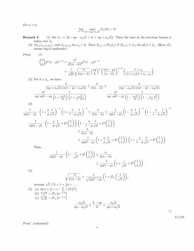
For a > 0,lim

n→∞max

|k−np|<a√

n|δn(k)| = 0.

Remark 5. (1) Set In := k : np − a√

n < k < np + a√

n. Then the max in the previous lemma istaken over In.

(2) (Sn,k)n>0,k∈Inand (tn)n>0 for tn > 0. Then Sn,k = Ou(tn) if |Sn,k| ≤ ctn for all k ∈ In. (Here, Ou

means big-O uniformly.)

Proof. (1)(n

k

)pk(1− p)n−k =

n!k!(n− k)!

pk(1− p)n−k

=1√2π

√n

k(n− k)

(np

k

)k(

n(1− p)(n− k)

)n−k ( 1 + εn

(1 + εk)(1 + εn−k)

).

(2) For k ∈ In, we haven

(np + a√

n) (n(1− p) + a√

n)≤ n

k(n− k)≤ n

(np− a√

n) (n(1− p)− a√

n)n

np ·n(1− p)1(

1 + a√

npn

)(1 + a

√n

(1−p)n

) n

np ·n(1− p)1(

1− a√

npn

)(1− a

1−p

√n

n

)(3)

1np(1− p)

·(

1 +a

p

1√n

)−1(1 +

a

1− p

1√n

)−1

≤ n

k(n− k)≤ 1

np(1− p)

(1− a

p

1√n

)−1(1− a

1− p

1√n

)−1

1np(1− p)

·(

1− a

p

1√n

+O(

1n

))(1− a

1− p

1√n

+O(

1n

))≤ n

k(n− k)

≤ 1np(1− p)

(1 +

a

p

1√n

+O(

1n

))(1 +

a

1− p

1√n

+O(

1n

))Thus,

1np(1− p)

·(

1− c√n

+O(

1n

))≤ n

k(n− k)

≤ 1np(1− p)

(1 +

c√n

+O(

1n

)).

(4) √n

k(n− k)=

1√np(1− p)

(1 +Ou

(1√n

)),

because√

1 + h = 1 + 12h + . . . .

(5) (a) ln(1 + t) = t− t2

2 +O(t3)

(b) k−npk = Ou

(n−1/2

)(c) k−np

n−k = Ou

(n−1/2

)−a√

n

np− a√

n≤ k − np

k≤ a

√n

np + a√

n

2/1/07

Proof. (continued)9

(6)

ln

((np

k

)k(

n(1− p)n− k

)n−k)

= k ln(

1− k − np

k

)+ (n− k) ln

(1 +

k − np

n− k

)= −1

2(k − np)2

(1k

+1

n− k

)+ kOu

(n−3/2

)+ (n− k)Ou

(n−3/2

)= −1

2(k − np)2

1np(1− p)

+Ou

(n−1/2

).

(7) (np

k

)k(

n(1− p)n− k

)n−k

= exp(− (k − np)2

2np(1− p)

)(1 +Ou

(n−1/2

)),

since

eOu(n−1/2) = 1 +Ou

(n−1/2

)and

eh = 1 + h +O(h2).

(8) εn < An , εk < A

k and εn−k < An−k . Also, 1

k = Ou

(1n

)and 1

n−k = Ou

(1n

). This means that

1 + εn

(1 + εk)(1 + εn−k)=(

1 +Ou

(1n

))1 + h1

(1 + h2)(1 + h3)= (1 + h1)

(1− h2 +O(h2

2)) (

1− h3 +O(h23))

= 1 +O(h1) +O(h2) +O(h3) + . . . .

(9) We combine the estimations from steps 3, 7 and 8 to get the statement of the Lemma.(n

k

)pk(1− p)n−k =

1√2πnp(1− p)

exp(− (k − np)2

2np(1− p)

)(1 +Ou

(n−1/2

)).

Lemma 3. Let [a, b] ⊆ R and f ∈ C0[a, b] with f(x) = 0 for x ∈ R \ [a, b]. Then for ε > 0, there existsh > 0 so that ∣∣∣∣∣h

+∞∑k=−∞

f(t + kh)−∫ b

a

f(x) dx

∣∣∣∣∣ < ε

for all t ∈ R.

Remark 6. Note that in the previous lemma, we may see that f is discontinuous at a and at b.Also, notice that h

∑+∞k=−∞ f(t + kh) looks a lot like a Riemann sum for the integral

∫ b

af(x) dx, however,

it overcounts near a and doesn’t take into account the stuff from t + kfinalh to b.

Proof. (1)

|f(x)− f(y)| < ε

for all x, y ∈ [a, b] with |x− y| < h.(2)

k ∈ Z : a ≤ t + kh ≤ b = i, i + 1, . . . , j − 1, j,

and M := sup[a,b] |f(x)|.10

(3) ∣∣∣∣∣∣∣∣h∑k∈Z

t+kh∈[a,b]

f(t + kh)−∫ b

a

f(x) dx

∣∣∣∣∣∣∣∣ ≤ hM +j∑

k=i

∣∣∣∣∣hf(t + kh)−∫ t+(k+1)h

t+kh

f(x) dx

∣∣∣∣∣+ 2hM

≤ 3hM + (j − i)hε

≤ 3hM + (b− a)ε.

Here, the hM term comes from not counting the hf(t + jh) term and the 2hM term comes from∫ t+ih

af(x) dx and

∫ b

t+jhf(x) dx.

Theorem 5 (Central Limit Theorem for Binomial Probabilities).

Proof. Let a, b be fine and set Kn :=[a√

np(1− p), b√

np(1− p)].

(1)

Pn [Sn − np ∈ Kn] =n∑

k=0

(χKn(k − np)) Pn [Sn = k]

=1√

2πnp(1− p)

n∑k=0

(χKn(k − np)) exp(− (k − np)2

2np(1− p)

)(1 + δn(k)) .

Recall that δn(k) = Ou

(n−1/2

).

(2) Pulling out the (1 + δn), we get

(1 + δn)1√

2πnp(1− p)

n∑k=0

(χKn(k − np)) exp

(− (k − np)2

2np(1− p)

)(1 + δn(k))

(3) For n 0, we can replace∑n

k=0 by∑

k∈Z. Then we get

Pn[Sn − np ∈ Kn]

=1√2π

1√np(1− p)

∑k∈Z

(χ[a,b]

(k√

np(1− p)−√

np

1− p

))exp

−12

(k√

np(1− p)−√

np

1− p

)2

(4) Set h = 1√np(1−p)

and f(x) = 1√2π

e−x22 and so

Pn[Sn − np ∈ Kn] −→ 1√2π

∫ b

a

e−x2/2 dx

as n →∞.

Let’s now show that Pn[Sn − np < b√

np(1− p)] −→ 1√2π

∫ b

−∞ e−x2/2 dx. Let b ∈ R and ε > 0 and c > 0

be such that 1√2π

∫ +∞c

e−x2/2 dx < ε and 1√2π

∫ −c

−∞ e−x2/2 dx < ε. Then∣∣∣∣∣Pn[Sn − np < b√

np(1− p)]− 1√2π

∫ b

−∞e−x2/2 dx

∣∣∣∣∣ ≤ An + Bn + C,

11

for An = Pn[Sn − np < −c√

np(1− p)] and Bn =∣∣∣∣Pn[−c ≤ Sn−np√

np(1−p)≤ b]− 1√

2π

∫ b

−ce−x2/2 dx

∣∣∣∣ and C =

1√2π

∫ −c

−∞ e−x2/2 dx. Note that C < ε and Bn < ε for n large by the previous theorem. Also,

0 ≤ An ≤ 1− Pn

[−c√

np(1− p) ≤ Sn − np ≤ c√

np(1− p)]

≤ 1−(

1√2π

∫ c

−c

e−x2/2 dx− ε

)= 1− 1√

2π

∫ c

−c

e−x2/2 dx + ε

= 2ε + ε

= 3ε.

2/6/07Confer Probability by L. Breiman.

Definition 6. F is the distribution of X if P[X < x] = F (x).

Let Xn and X be random variables.

Definition 7 (8.2). Xn converges to X in distribution, written XnD−→ X, if Fn(x) −→ F (x) at every point

x where F is continuous. Sometimes this is written FnD−→ F .

(Note that convergence in distribution is equivalent to convergence in measure, where the measure µ isdefined to be µ ((a, b]) = F (b)− F (a).)

Definition 8 (8.26). If F (x) is a cdf, then the characteristic function is defined to be

f(u) =∫

eiuxF (dx) = E[eiux].

(This is a Riemann-Stieltjes integral.)

Notice that this is really a Fourier transform of measure.

Theorem 6 (Continuity Theorem (8.28)). Suppose that Fn are distribution functions with characteristicfunctions fn. Suppose that limn→∞ fn(u) exists for all u and limn→∞ fn(u) = h(u). Then there is adistribution function F so that Fn

D−→ F and h(u) is the characteristic function of F .

Theorem 7 (Separation Theorem (8.24); restated). No two distinct distribution functions have the samecharacteristic function.

The Separation Theorem is not really a uniqueness theorem, but is rather a “one-to-one-ness” theorem.

Proposition 7 (8.33). Let X1, . . . , Xn be random variables with characteristic functions f1(u), . . . , fn(u).Then the random variables are independent if and only if

E

(exp[i

n∑k=1

ukXk]

)=

n∏k=1

fk(uk).

If X is a random variable with distribution function FX and characteristic function fX(u) and Y is a ran-dom variable with distribution function FY and characteristic function fY (u) and X and Y are independent,then X + Y is a random variable with distribution function

FX ∗ FY =∫

FX(x− y)FY (dy)

and characteristic functionfX(u)FY (u).

12

Distribution Function Characteristic Function

FX , FY , FX ∗ FY..fX , fY , fXfY

F1, F2, . . .D−→ F

..f1, f2, . . .

pointwise−→ f

FX-- fX

FY-- fY

Proposition 8 (8.44). If E|X|k < ∞, then the characteristic function of X has expansion

f(u) =k−1∑j=0

(iu)j

j!E[Xj ] +

(iu)k

k!(E[Xk] + δ(u)

)and limu→0 δ(u) = 0 with

|δ(u)| ≤ 3E[|X|k].

(This is really just a Taylor expansion.)

Theorem 8 (Central Limit Theore (9.2)). Suppose that X1, X2, . . . are independent random variables withE[Xk] = 0 and E[X2

k ] = σ2k < ∞ and that (sn)2 =

∑nk=1 σ2

k. Finally suppose that lim supn1

s3n

∑nk=1 E[|Xk|3] =

0. Then we see thatSn

sn=

X1 + · · ·+ Xn

sn

D−→ X,

where X ∼ N(0, 1).

Recall that N(0, 1) means normal with mean 0 and standard deviation 1.

Proof. Let fk(u) be fXkand gn be the characteristic function of Sn

sn= X1+···+Xn

sn(where sn =

√∑nk=1 σ2

k).Then

gn(u)(8.33)=

n∏k=1

fk

(u

sn

)=

n∏k=1

(1 +

(fk

(u

sn

)− 1))

.

Note that by (8.44) we have

fk

(u

sn

)= 1− u2

2

(σ2

k + δk

(u

sn

)).

By the triangle inequality, we have∣∣∣∣fk

(u

sn

)− 1∣∣∣∣ ≤ u2

2

(σ2

k + 3E[x2

k

s2n

])≤ 2u2σ2

k

s2n

.

Now concerning the expected value, we have[E(|Xk|2

)]3/2 ≤ E[X3

k

]by Jensen’s Inequality. Since the left-hand side is σ3

k, we see that

σ3k ≤ E

[X3

k

].

Claim 2. The hypothesis on the lim sup implies that

supk≤n

σk

sn−→ 0.

13

So we see that supk≤n |fk(u/sn)− 1| −→ 0 as n →∞. Now we can also see that log(1 + z) = z + θz2 for|θ| ≤ 1 for |z| ≤ 1

2 . Then we have

log gn(u) =n∑

k=1

(fk

(u

sn

)− 1)

+ θn∑

k=1

(fk

(u

sn

)− 1)2

Then we have ∣∣∣∣∣θn∑

k=1

(fk

(u

sn

)− 1)2∣∣∣∣∣ Cauchy-Schwarz

≤ supk≤n

[∣∣∣∣fk

(u

sn

)− 1∣∣∣∣] · n∑

k=1

∣∣∣∣fk

(u

sn

)− 1∣∣∣∣

≤ supk≤n

[∣∣∣∣( u

sn

)− 1∣∣∣∣] · n∑

k=1

2u2σ2k

s2n

≤ 2u2 supk≤n

[∣∣∣∣fk

(u

sn

)− 1∣∣∣∣]

Thus,

supk≤n

∣∣∣∣fk

(u

sn

)− 1∣∣∣∣ −→ 0

as n →∞. Notice that

fk

(u

sn

)− 1 = −u2

2σ2

k

s2n

+ θku3

s3n

E[|Xk|3

] claim−→ 0.

Thus,n∑

k=1

(fk

(u

sn

)− 1)

= −u2

2

n∑k=1

σ2k

s2n

+u3∑n

k=1 θkE[|Xk|3

]s2

n

claim−→n→∞

−u2

2and so we are done up to proving the claim.

2/8/07Remember that we had the condition

lim supn

1s3

n

n∑k=1

E[|Xk|3

]= 0

for the Central Limit Theorem. Let’s consider the case where

Xk =

1− p, p

−p, 1− p

for the (recentered) Bernoulli Random Variable. (Notice that the Bernoulli Random Variable is usually 1with probability p and 0 with probability 1− p instead of 1− p with probability p and −p with probability1− p.) Then we have

E[|X|3

]= (1− p)3p + p3(1− p)

= p(1− p)((1− p)2 + p2

)= p(1− p)(1− 2p + 2p2),

and

s2n = np(1− p)

sn =√

np(1− p)

s3n = n3/2 (p(1− p))3/2

.

14

Putting all of this together, we have

1s3

n

n∑k=1

E[|X|3

]=

np(1− p)(1− 2p + 2p2)

n3/2 (p(1− p))3/2=

C

n1/2,

and so the condition is verified.

Theorem 9 (Berry-Eseen Theorem). Suppose Sn = X1 + · · · + Xn are indpendent, identically distributedrandom variables. Suppose that E[Xk] = 0 and E[X2

k ] = σ2 < ∞ and E[|X|3

]< ∞. If Φ is a cumulative

distribution function of N (0, 1), then

supx

∣∣∣∣P [ sn

σ√

n< x

]− Φ(x)

∣∣∣∣ ≤ cE[|Xk|3

]σ3√

n

for c ≤ 4.

3.2. Heuristics About Why We Have N (0, 1). Assume that Zn = X1+···+Xn√n

D−→ X. What must X be

like? Note that Z2n = X1+···+Xn+Xn+1+···+X2n√2n

and we must have Z2nD−→ X. Rewriting this, we have

Z2n =X1 + · · ·+ Xn√

2√

n+

Xn+1 + · · ·+ X2n√2√

n=

1√2

(Z ′n + Z ′′n) .

Assume independence of all of the random variables. Then Z ′n is independent of Z ′′n and Z ′nD−→ X and Z ′′n

D−→X. The limit random variables must satisfy X = 1√

2(X ′ + X ′′), where = means the same distribtution and

X, X ′ and X ′′ are three realizations of the random variable with common distribution.

Proposition 9 (9.1). If X is a random variable and E[X2]

= σ2 < ∞ and XD= X′+X′′

√2

for X ′ and X ′′

are independent and X, X ′ and X ′′ all share the same distribution, then X has a N (0, σ2) distribution.

Remark 7. This is what is meant by the normal distribution having a sort of self-similarity. We can taketwo copies of it and properly normalize and we get the normal distribution back.

Proof. Note that X1, X2, . . . are independent identically distributed as X. We also see that E[X] = 0 since

E[X] =E[X ′] + E[X ′′]√

2=√

2E[X].

By iteration,

XD=

X1 + · · ·+ X2m

2m/2

D−→CLT

Z,

for Z ∼ N (0, σ2).

Claim 3. lim supn1

s3n

∑nk=1 E[|Xk|3] implies that supk≤n

σk

sn−→ 0 as n →∞.

Proof. We knew from before that σ3k ≤ E[X3

k ] ≤ E[|Xk|3]. Then we see that lim supn1

s3n

∑nk=1 σ3

k = 0. So for

sufficiently large N , we have that for all n ≥ N supj≥n1s3

j

∑jk=1 σ3

k < 1. Assume, toward a contradiction,

that supk≤nσ3

k

s3n6−→ 0 as n →∞. Then there exists ε0 > 0 so that for all j there exists k ∈ 1, . . . , j so that

σ3k

s3j≥ ε0. Then we see that

limn→∞

supj≥n

j∑k=1

σ3k

s3j

= lim sup

j∑k=1,( 6=k2)

σ3k

s3j

+σ3

k

s3j

= lim sup

j∑k=1,( 6=k2)

σ3k

s3j

+ ε0

> 0,

15

which is a contradiction. Thus, supk≤nσ3

k

s3n−→ 0 as n →∞ and so supk≤n

σk

sn−→ 0 as n →∞.

4. Chapter 8: Moderate Deviations Theorem

Theorem 10 (Cramer, 1938). Suppose we have a sequence an with limn→∞ an = ∞ and limn→∞an

n1/6 = 0.Then

Pn

[sn

n− p ≥

√p(1− p)

an√n

]∼ 1

an

√2π

e−a2n/2.

Proposition 10. For 0 ≤ k ≤ n set(n

k

)pk(1− p)n−k =

1√2πnp(1− p)

exp(−(k − np)2

2np(1− p)

)· (1 + δn(k)) .

For every positive real sequence cn such that cn → 0,

limn→∞

max|k−np|<cnn2/3

|δn(k)| = 0.

2/13/07

Proposition 11 (“Optimization”/extension of DeMoivre-Laplace Theorem). For 0 ≤ k ≤ n, set(n

k

)pk(1− p)k =

1√2πp(1− p)n

exp(−(k − np)2

2np(1− p)

)(1 + δn(k)).

Let J ′n = k ∈ Z : |k − np| < cnn2/3. Then for every positive real sequence cn with cn −→n→∞

0 we have

limn→∞

maxk∈K

|δn(k)| = 0.

Proof. Recall from the DeMoivre-Laplace Theorem that(nk

)−→

√n

k(n−k) . Then we have

n

(np + cnn2/3)(n(1− p) + cnn2/3)≤ n

k(n− k)≤ n

(np− cnn2/3)(n(1− p)− cnn2/3)1n· 1(p + cnn−1/3)((1− p) + cnn−1/3)

≤ n

k(n− k)≤ 1

n· 1(p− cnn−1/3)((1− p)− cnn−1/3)

1np(1− p)

· 1(1 + cnn−1/3

p

)(1 + cnn−1/3

1−p

) ≤ n

k(n− k)≤ 1

np(1− p)· 1(

1− cnn−1/3

p

)(1− cnn−1/3

1−p

)

n

k(n− k)=

1np(1− p)

·(1 +Ou(cnn−1/3)

)√

n

k(n− k)=

1√np(1− p)

·(1 +Ou(cnn−1/3)

).(a)

Note that k−npk = Ou(cnn−1/3) and k−np

n−k = Ou(cnn−1/3).

ln

[(n

kp)k(

n

n− k(1− p)

)n−k]

= −12(k − np)2

(1k

+1

n− k

)+ kOu(c3

nn−1) + (n− k)Ou(c3nn−1)

= −12(k − np)2

1np(1− p)

+Ou(c3n).(b)

Thus, we see that (np

k

)k(

n(1− p)n− k

)n−k

= exp(−(k − np)2

2np(1− p)

)(1 +Ou(c3

n)).

16

In the DeMoivre-Laplace Theorem (or Lemma) we had

(c)1 + εn

(1 + εk)(1 + εn−k)=(

1 +Ou

(1n

)).

Now combining parts (a), (b) and (c) above, we get(n

k

)pk(1− p)n−k =

1√2πp(1− p)n

exp(−(k − np)2

2np(1− p)

)(1 +Ou(c′n)) ,

where c′n = max(cnn−1/3, c3

n, n−1).

Proposition 12. Consider two sequences kn and `n where kn < `n for all n and kn = np + o(n2/3) and`n = n(1− p) + o(n2/3); i.e., kn = np + c′nn2/3 where c′n −→

n→∞0 and `n = n(1− p) + c′′nn2/3 where c′′n −→

n→∞0.

Then as n →∞ we have

Pn (kn ≤ Sn ≤ `n) ∼ 1√2π

∫ bn

an

e−x2/2 dx,

where an = kn−np√np(1−p)

and bn = `n−np√np(p(1−p))

.

Proof. Let h(n) = 1√np(1−p)

. Take n so large that 0 ≤ kn < `n ≤ n. Then

Pn(Sn = j) =h(n)√

2πexp

(−(j − np)2

2np(1− p)

)(1 + δn(j)).

and

(1) Pn (kn ≤ Sn < `n) =h(n)√

2π

`n−1∑j=kn

exp(−(j − np)2

2np(1− p)

)(1 + δn(j)).

It suffices to show that

h(n)`n−1∑j=kn

exp(−(j − np)2

2np(1− p)

)∼∫ bn

an

e−x2/2 dx.

(This will require proof next time.)

Claim 4.

h(n)exp(−(j − np)2

2np(1− p)

)−∫ bn

an

e−x2/2 dx = o

(∫ bn

an

e−x2/2 dx

)

2/15/07

Remark 8. Note that if xn ∼ yn and yn ∼ zn, then xn ∼ zn.

Let’s finish the proof from last time. Given the claim, divide equation (1) by 1√2π

∫ bn

ane−x2/2 dx on the

right hand side, subtract 1 and take absolute values and use the triangle inequality to get∣∣∣∣∣∣h(n)√

2π

∑`n−1j=kn

exp(−(j−np)2

2np(1−p)

)1√2π

∫ bn

ane−x2/2 dx

+

h(n)√2π

∑`n−1j=kn

exp(−(j−np)2

2np(1−p)

)1√2π

∫ bn

ane−x2/2 dx

− 1

∣∣∣∣∣∣≤

∣∣∣∣∣∣h(n)√

2π

∑`n−1j=kn

exp(−(j−np)2

2np(1−p)

)1√2π

∫ bn

ane−x2/2 dx

− 1

∣∣∣∣∣∣+ maxj|δn(j)|

∣∣∣∣∣∣h(n)√

2π

∑`n−1j=kn

exp(−(j−np)2

2np(1−p)

)1√2π

∫ bn

ane−x2/2 dx

∣∣∣∣∣∣−→ 1,

because maxj δn(j) −→ 0. So if the claim is true, then the proposition is proved.17

Let xn(j) = j−np√np(1−p)

. No assume that an > 0. Then we have

h(n)exp(−xn(j + 1)2

2

)<

∫ xn(j+1)

xn(j)

e−x2/2 dx < h(n)exp(−xn(j)2

2

).

The left hand side gives us essentially the right-box Riemann sum approximation, while the right hand sideessentially gives us the left-box approximation. Then we get

(2) 0 ≤ h(n)ln−1∑j=kn

e−xn(j)2/2 −∫ bn

an

e−x2/2 dx ≤ h(n)(e−a2

n/2 − e−b2n/2)

.

Also,

(3)∫ bn

an

e−x2/2 dx ≥ 1bn

∫ bn

an

xe−x2/2 dx =1bn

(e−a2

n/2 − e−b2n/2)

.

Now dividing (3) by (2), we get

h(n)∑ln−1

j=kne−xn(j)2/2 −

∫ bn

ane−x2/2 dx∫ bn

ane−x2/2 dx

≤ h(n)bn

Theorem 11 (Moderate Deviations Result). Suppose (an) is a sequence of real numbers such that an −→n→∞

∞and limn→∞

an

n1/6 = 0. Then

Pn

[Sn

n− p ≥

√p(1− p)

an√n

]∼ 1

an

√2π

e−a2n/2.

Proof. (1) Note that an −→∞ less quickly than n1/6.(2) Let dn =

√an. Then limn→∞

dn

an= 0 and so dn = o(an).

(3) Let kn = dnp +√

np(1− p)ane and `n = dnp +√

np(1− p)(an + dn)e. A picture of where things siton the number line is below:

-

np +√

np(1− p)an

kn `n

(4) Event (Sn ≥ kn) =(

Sn

n − p ≥ kn

n − p)

=(

Sn

n − p ≥√

p(1−p)√n

an

). Thus,

Pn

[Sn

n− p ≥

√p(1− p)√

nan

]= Pn [Sn ≥ kn] = Pn [kn ≤ Sn ≤ `n]︸ ︷︷ ︸

(5) takes care of this

+ Pn [Sn ≥ `n]︸ ︷︷ ︸(8) takes care of this

.

(5) Now, an = o(n1/6) and so kn, `n = np + o(n2/3). From the last proposition, set

a′n =kn − np√np(1− p)

, bn =`n − np√np(1− p)

,

and so

Pn [kn ≤ Sn < `n] ∼ 1√2π

∫ bn

a′n

e−x2/2 dx.

This allows us to say that

Pn [kn ≤ Sn < `n] ∼ 1√2π

∫ bn

an

e−x2/2 dx︸ ︷︷ ︸(6) takes care of this

− 1√2π

∫ a′n

an

e−x2/2 dx.︸ ︷︷ ︸(7) takes care of this

18

(6) We will show that ∫ bn

an

e−x2/2 dx ∼ 1an

e−a2n/2.

(a) Notice that ∫ bn

an

e−x2/2 dx ≤ 1an

∫ ∞

an

xe−x2/2 dx =1an

e−a2n/2.

(b) We also have that bn ≥ an + dn, since normalizint the ceiling is bigger than normalizing theargument of the ceiling. Thus,∫ bn

an

e−x2/2 dx ≥∫ an+dn

an

e−x2/2 dx

≥ 1an + dn

∫ an+dn

an

xe−x2/2 dx

=1

an + dn

(exp

(−a2

n

2

)− exp

(−(an + dn)2

2

)).

Divide by 1an

exp(−a2

n

2

)to get on the right hand side:

=an

an + dn− an

an + dn

exp(−(an+dn)2

2

)exp

(−a2

n

2

)−→ 1− 0 = 1.

Now combine 6(a) and 6(b) to get the result in 6.(7) We will show that ∫ a′n

an

e−x2/2 dx = o

(1an

e−a2n/2

).

Note that ∫ a′n

an

e−x2/2 dx ≤ 1√np(1− p)

exp(−a2

n

2

).

Divide through by 1an

exp(−a2

n

2

).∫ a′n

ane−x2/2 dx

1an

exp(−a2

n

2

) <an√

np(1− p)−→ 0,

since an = o(n1/6).(8) We will show that

Pn [Sn ≥ `n] = o

(1an

e−a2n/2

).

(a) By the Large Deviations Theorem we have

Pn [Sn ≥ `n] ≤ exp(−nh+

(√p(1− p)

bn√n

)),

where h+(ε) = ε2

2p(1−p) +O(ε3) for ε −→ 0. Thus,

Pn [Sn ≥ `n] exp(−b2

n

2+O

(b3n√n

))∼ exp

(−b2

n

2

),

since bn = o(n1/6).19

(b) Notice that

exp(−b2

n

2

)≤ exp

(−(an + dn)2

2

)= o

(exp

(−d2

n

2

)exp

(−a2

n

2

)).

(c) We can see that exp(−d2

n

2

)≤ 1

anby our choice of dn. (Note that dn >

√2 ln an.)

This concludes step 8.

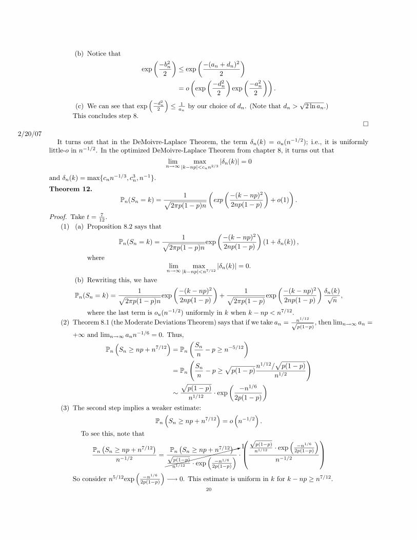
2/20/07It turns out that in the DeMoivre-Laplace Theorem, the term δn(k) = ou(n−1/2); i.e., it is uniformly

little-o in n−1/2. In the optimized DeMoivre-Laplace Theorem from chapter 8, it turns out that

limn→∞

max|k−np|<cnn2/3

|δn(k)| = 0

and δn(k) = maxcnn−1/3, c3n, n−1.

Theorem 12.

Pn(Sn = k) =1√

2πp(1− p)n

(exp

(−(k − np)2

2np(1− p)

)+ o(1)

).

Proof. Take t = 712 .

(1) (a) Proposition 8.2 says that

Pn(Sn = k) =1√

2πp(1− p)nexp

(−(k − np)2

2np(1− p)

)(1 + δn(k)) ,

wherelim

n→∞max

|k−np|<n7/12|δn(k)| = 0.

(b) Rewriting this, we have

Pn(Sn = k) =1√

2πp(1− p)nexp

(−(k − np)2

2np(1− p)

)+

1√2πp(1− p)

exp(−(k − np)2

2np(1− p)

)δn(k)√

n,

where the last term is ou(n−1/2) uniformly in k when k − np < n7/12.(2) Theorem 8.1 (the Moderate Deviations Theorem) says that if we take an = n1/12√

p(1−p), then limn→∞ an =

+∞ and limn→∞ ann−1/6 = 0. Thus,

Pn

(Sn ≥ np + n7/12

)= Pn

(Sn

n− p ≥ n−5/12

)= Pn

(Sn

n− p ≥

√p(1− p)

n1/12/√

p(1− p)n1/2

)

∼√

p(1− p)n1/12

· exp(

−n1/6

2p(1− p)

)(3) The second step implies a weaker estimate:

Pn

(Sn ≥ np + n7/12

)= o

(n−1/2

).

To see this, note that

Pn

(Sn ≥ np + n7/12

)n−1/2

=:1Pn

(Sn ≥ np + n7/12

)√

p(1−p)

n1/12 · exp(−n1/6

2p(1−p)

) ·√

p(1−p)

n1/12 · exp(−n1/6

2p(1−p)

)n−1/2

So consider n5/12exp

(−n1/6

2p(1−p)

)−→ 0. This estimate is uniform in k for k − np ≥ n7/12.

20

(4) Note that

exp(−(k − np)2

2np(1− p)

)≥ exp

(−n14/12

2np(1− p)

)= exp

(−n1/6

2p(1− p)

)−→

n→∞0,

and exp(−(k−np)2

2np(1−p)

)= o(1).

(5) Thus, we see that1√

2πp(1− p)nexp

(−(k − np)2

2np(1− p)

)= o(n−1/2)

uniformly in k with k − np ≥ n7/12.(6) Make step 3 look the same as 1b by throwing 5 into 3 without disturbing the estimate:

Pn (Sn = k) =1√

2πp(1− p)nexp

(−(k − np)2

2np(1− p)

)+ o(n−1/2).

Finally, factor out 1√2πp(1−p)n

and you’ve finished the proof.

Consider

Yn =

1, p

−1, 1− p,

and Mn =∑n

j=1 Yj . Note that Mn = 2Sn − n. This the the gambler’s net gain or loss or a random walk.

Proposition 13.

Pn (Mn = k) =

√2π

(p

1− p

)k/2 (2√

p(1− p))n

√n

(exp

(−k2

2n

)+ o(1)

).

Corollary 2. Let K be a fixed finite subset of Z that contains at least one even and one odd number. Then

limn→∞

1n

ln (Pn [Mn ∈ K]) = ln(2√

p(1− p))

.

Proof. (of Proposition 13)Let p = 1

2 in Theorem 9.1. Then

Pn (Sn = k) =1√

2π 14n

[exp

(−(k − n/2)2

2n 14

)+ o(1)

]

=

√2π

1√n

[exp

(−2n

(k − n

2

)2)

+ o(1)]

For p ∈ (0, 1) \ 1/2, we have

Pn (Sn = k) =(

n

k

)pk (1− p)n−k

=

√2π

1√n

2npk(1− p)n−k

[exp

(−2n

(k − n

2

)2)

+ o(1)]

=

√2π

2/27/07

Definition 9. Set Tn = |k : 0 ≤ k ≤ n, Mk > 0| and T ′n = |k : 1 ≤ k ≤ n, Mk > 0 or Mk−1 > 0|.21

Our line segments of a path are in the upper half plane if and only if M2k−1 > 0. Thus, we can say

T ′2n = 2 |k : 1 ≤ k ≤ n and M2k−1 > 0| .

Proposition 14. For each n > 0 and 0 ≤ k ≤ n, then

P2n [T ′2n = 2k] = 2−2n

(2k

k

)(2(n− k)n− k

)Proof. Note that

P2n [T ′2n = 2n] = P2n [Mk ≥ 0, k ∈ 1, . . . , 2n] =Cor. 10.5

2−2n

(2n

n

).

We proceed by induction. The base case where n = 1 is that

P2[T ′2 = 0] =12

= 2−2(1)

(2(0)0

)(2(1− 0)

1

)=

12

P2[T ′2 = 2] =12.

Our inductive hypothesis is that the proposition is true for all n ≤ N − 1 and for all 0 ≤ k ≤ n. Notethat if k = 0, we have

P2n [T ′2n = 0] = P2n [Mk ≤ 0, ∀k] =Cor. 10.5

2−2N

(2N

N

).

Now if 0 < T ′2N < 2N , then there exists j with 1 ≤ j ≤ N so that M2j = 0. For each ω ∈ Ω2N so that0 < T ′2n(ω) < 2N , the first time back to 0 is given by

t = t(ω) := minj > 0 : M2j(ω) = 0.

Fix k ∈ 1, . . . , N − 1. Then

P2N [T ′2N = 2k] =N∑

j=1

P2N [T ′2N = 2k, t(ω) = 2j, M1 > 0]

+N∑

j=1

P2N [T ′2N = 2k, t(ω) = 2j, M1 < 0]

If j > k, then note thatT ′2N = 2k, t(ω) = 2j, M1 > 0 = ∅.

Note that

|T ′2N = 2k, t(ω) = 2j, M1 > 0| = ( # of paths (0, 0) −→ (2j, 0) with Mi > 0 for i > 1)

× (# of paths starting at (2j, 0) and length 2(N − j)

with 2(k − j) elementary segmenst in the UHF)

The first term in the product is given by 10.6 and is 1j

(2j−2j−1

)and the second term is

22(N−j)P[T ′2(N−j) = 2(k − j)

]=(

2(k − j)k − j

)(2(N − k)N − k

).

3/6/07

Proof. Thus, we see that

P2N (T ′2N = 2k, t(ω) = 2j,M1 > 0) =1

j22N

(2j − 2j − 1

)(2(k − j)k − j

)(2(N − k)N − k

).

22

Now combining the results we have

P2N (T ′2N = 2k) =k∑

j=1

1j22N

(2j − 2j − 1

)(2(k − j)k − j

)(2(N − k)N − k

)+

k∑j=1

1j22N

(2j − 2j − 1

)(2k

k

)(2(N − j − k)N − j − k

)

=[

122N

(2(N − k)N − k

)] k∑j=1

1j

(2j − 2j − 1

)(2(k − j)k − j

)+[

122N

(2k

k

)] k∑j=1

1j

(2j − 2j − 1

)(2(N − j − k)N − j − k

)

=[

122N

(2(N − k)N − k

)](12

)(2k

k

)+[

122N

(2k

k

)](12

)(2(N − k)N − k

)=

122N

(2k

k

)(2(N − k)N − k

),

which means that induction holds and so we have proven Proposition 10.8.

3/8/07Theorem 13 (10.1 Arcsine Law). For each α ∈ (0, 1),

Pn(Tn < nα) −→ 1π

∫ α

0

1√x(1− x)

dx =2π

arcsin√

α.

Example 2.

Pn[Tn ≥ .85n] = 1− Pn[Tn < .85n] −→n→∞

1− 2π

arcsin√

.85 = .25318.

Proposition 15 (10.9). For all a, b with 0 ≤ a ≤ b ≤ 1, then

limn→∞

P2n [2na ≤ T ′2n ≤ 2nb] =1π

∫ b

a

1√x(1− x)

dx.

Proof. (1) First, if we have 0 < a < b < 1, then by Proposition 10.8 and Stirling’s Approximation tellus

P [T ′2n = 2k] =1π

1√k(n− k)

(1 + ε(k)) (1 + ε(n− k))

=1π

1√k(n− k)

(1 + ε(n, k)) .

With limn→∞ ε(n, k) = 0 uniformly in k ∈ Z for a ≤ k ≤ nb. Thus, we have

P2n [2na ≤ T ′2n ≤ 2nb] =∑

na≤k≤nb

P [T ′2n = 2k]

∼∑

a≤ kn≤b

1π

1√k(n− k)

=∑

a≤ kn≤b

1π

1√n2(

kn

) (1− k

n

)=

n∑k=0

(χ[a,b]

(k

n

))1π

1n

1√(kn

) (1− k

n

)=

1nπ

n∑k=0

(χ[a,b]

(k

n

))1√(

kn

) (1− k

n

)−→ 1

π

∫ 1

0

χ[a,b]1√

x(1− x)dx

−→ 1π

∫ b

a

1√x(1− x)

dx.

23

Note that here we actually have a Riemann sum since we have a bounded function when we keepa 6= 0 and b 6= 1. The rest of this proof is really to allow a = 0 and b = 1.

(2) Fix ε > 0. There exists an a so that 1π

∫ a

01√

x(1−x)dx < ε and 1

π

∫ 1

1−a1√

x(1−x)< ε. From part (1) of

the proof, we have∣∣∣∣∣ 1π∫ 1−a

a

1√x(1− x)

dx− P2n [2na ≤ T ′2n ≤ 2n(1− a)]

∣∣∣∣∣ < ε

for n 0.(3) Note that P2n [T ′2n < 2na] + P2n [2na ≤ T ′2n ≤ 2n(1− a)] + P2n [T ′2n > 2n(1− a)] = 1. Note that

1π

∫ 1

01√

x(1−x)dx = 1 implies that

1π

∫ 1−a

a

1√x(1− x)

dx = 1−∫ a

0

1√x(1− x)

dx−∫ 1

1−a

1√x(1− x)

dx,

or in other words,

P2n [2na ≤ T ′2n ≤ 2n(1− a)] = 1− P2n [T ′2n < 2na]− P2n [T ′2n > 2n(1− a)] .

From these facts and part (2) we have∣∣∣∣∣(

1π

∫ a

0

1√x(1− x)

dx +1π

∫ 1

1−a

1√x(1− x)

dx− 1

)+ (1− P2n [T ′2n < 2na]− P2n [T ′2n > 2n(1− a)])

∣∣∣∣∣ < ε

for large enough n. Thus, for n 0 we have

|P [T ′2n < 2na] + P2n [T ′2n > 2n(1− a)]| < 3ε.

So there exists a > 0 so that P2n [T ′2n < 2na] < 3ε for n 0. Since P2n [T ′2n < 2na] is increasing ina for fixed n, we get lima→∞ P2n [T ′2n < 2na] = 0 uniformly in n.1

(4) By part (1) and the above, we have

limn→∞

P [T ′2n ≤ 2nb] =1π

∫ b

0

1√x(1− x)

dx

for b ∈ (0, 1). By symmetry, the proposition holds.

Proof. (of Theorem 10.1)Since T2n := T ′2n − |k : 1 ≤ k ≤ n, M2k−1 > 0, M2k = 0|, we see that

(4) |T2n − T ′2n| ≤ |k : 1 ≤ k ≤ n, M2k = 0| = U2n.

By the Law of Returns to the Origin, we get

limn→∞

P2n [U2n > 2nε] = 0.

Alternatively, if we don’t use the Law of Returns to the Origin, note that

E [U2n] = E

[n∑

k=1

χ[M2k=0]

]

=n∑

k=1

P2n [M2k = 0]

=n∑

k=1

e−2k

(2k

k

).

By Markov’s Inequality,

P [U2n > 2nε] ≤ E [U2n]2nε

=1

2nε

n∑k=1

2−2k

(2k

k

).

1We can’t see why this is true right now, but we will come back to it later.24

By Stirling’s Approximation, we have limk→∞ 2−2k(2kk

)= 0 as 1√

n. Cesaro’s Principle gives

(5) limn→∞

P2n [U2n > 2nε] = 0.

3/27/07Recall that we had

T2n = T ′2n − |k : 1 ≤ k ≤ n, M2k−1 > 0, M2k = 0|and

(6) |T2n − T ′2n| ≤ |k : 1 ≤ k ≤ n and M2k = 0| = U2n.

We also knew that

E2n[U2n] = E

[n∑

k=1

χM2k=0

]=

n∑k=1

P2n(M2k = 0) =n∑

k=1

2−2k

(2k

k

).

Markov’s Inequality says

P[U2n > 2nε] ≤ E[U2n]2nε

=1

2nε

n∑k=1

2−2k

(2k

k

).

By Stirling’s Formula, we have that limn→∞ 2−2k(2kk

)= 0. Finally, Cesaro’s Principle gives us that

(7) limn→∞

P[U2n > 2nε] = 0.

Proof. (continued)Now note that

[T2n < 2nα] ⊂ [|T2n − T ′2n| > 2nε] ∪ [T ′2n ≤ 2n(α + ε)] .Thus, we have

(8) P[T2n < 2nα] ≤ P [|T2n − T ′2n| > 2nε] + P [T ′2n ≤ 2n(α + ε)] .

For the first probability on the right and Equations (6) (7), we have

P [|T2n − T ′2n| > 2nε] ≤ P [U2n > 2nε] −→ 0.

For the second probability on the right in Equation (8), note that Proposition 10.9 says that

limn→∞

P2n [T ′2n ≤ 2n(α + ε)] = limn→∞

P2n [T ′2n ≤ 2n(α + ε)]

=1π

∫ α+ε

0

1√x(1− x)

dx,

and ε −→ 0 gives

limε→0

1π

∫ α+ε

0

1√x(1− x)

dx =1π

∫ α

0

1√x(1− x)

dx.

Therefore going back to the left hand side of Equation (8), we have

lim supn→∞

P [T2n < 2nα] ≤ 1π

∫ α

0

1√x(1− x)

dx.

Since T2n ≤ T ′2n, Proposition 10.9 says that

lim infn→∞

P2n [T2n < 2nα] ≥ 1π

∫ α

0

1√x(1− x)

dx.

Thus, we get that limn→∞ P2n [T2n < 2nα] = 1π

∫ α

01√

x(1−x)dx. To complete, note that

P2n+1 [T2n+1 < (2n + 1)α] ≤ P2n [T2n < (2n + 1)α]

and similarly,P2n+2 [T2n+2 < (2n + 2)α] ≥ P2n+1 [T2n+1 < (2n + 2)α] .

25

Proposition 16 (Possibly Cesaro’s Principle). Assume that an∞1 is increasing and an −→ L as n →∞.Then

limn→∞

1n

n−1∑j=1

aj = L.

Theorem 14 (10.2).

Pn

[Un < α

√n]−→

n→∞

√2π

∫ α

0

e−x2/2 dx.

Remark 9. Note that the limit in the above theorem is erf(

α√2

).

Also, recall that U2n = |k : 1 ≤ k ≤ n, M2k = 0|.

Proposition 17 (10.10).

P2n [U2n = k] =1

22n−k

(2n− k

n

).

Proof. (1) Note that P2n [U2n = 0] = 2−2n(2nn

)by Proposition 10.4 using the second part and doubling

to account for symmetry.(1.5) Establis the base case where n = 1 and k = 0, 1. Next assume that this is true for all m < n with

0 ≤ k ≤ m. Notice that

P2 [U2 = 0] =12

=1

22−0

(21

)P2 [U2 = 1] =

12

=1

22−1

(11

).

(2) We will now proceed by induction. Suppose that U2n(ω) > 0. Then there exists j ≥ 1 so thatM2j(ω) = 0 and M2i(ω) 6= 0 for i < j. Let t(ω) = j. Then we see that

P2n [U2n = k] =n∑

j=1

P2n [t = j and U2n = k] .

(3) Note that j is even and if j > n− k + 1 then ω : t = j and U2n = k = ∅. If, j ≤ n− k + 1, then

ω : t = j and U2n = k = (paths from (0, 0) to (2j, 0) not touching the axis in between)

× (paths from (2j, 0) of length 2n− 2j, touching the axis k times) .

(4) Notice that

|ω : t = j, U2n = k| = 2j

(2j − 2j − 1

)2k−1

(2n− 2j − k + 1

n− j

).

(5) Note that

|U2n = k| = 2kn−k+1∑

j=1

1j

(2j − 2j − 1

)(2n− 2j − k + 1

n− j

).

(6) Lemma 10.7 says that

|U2n = k| = 2k

(2n− k

n

).

(7) Divide by 22n to get P [U2n = k].

3/29/07

Theorem 15.

Pn

[Un < α

√n]−→

n→∞

√2π

∫ α

0

e−x2/2 dx.

26

Proof. (1)

P2n [U2n = k] =1

22n−k

(2n− k

n

)=

122n−k

(2n− k)!n!(n− k)!

=1

22n−k

√2π(2n− k)1/2(2n− k)2n−k

e−(2n−k)(1 + ε2n−k)

√2πn1/2nne−n(1 + εn)

√2π(n− k)1/2(n− k)(n−k)

e−(n−k)(1 + ε(n−k))

=1√2π

√2n− k

n(n− k)

(1− k

2n

)n(1 +

k

2(n− k)

)n−k (1 +Ou

(1n

))(9)

(1.25) √2n− k

n(n− k)=

√2− k/n

n(1− k/n)=

√2n

(1 +Ou

(1√n

)).

(1.75)

ln

[(1− k

2n

)n(1 +

k

2(n− k)

)n−k]

= n ln(

1− k

2n

)+ (n− k) ln

(1 +

k

2(n− k)

)

= n

(− k

2n− k2

8n2+O

((k

2n

)3))

+ (n− k)

(k

2(n− k)− k2

8(n− k)2+O

((k

2(n− k)

)3))

=−k2

8n− k2

8(n− k)+O (?)

= − k2

4n

(1 +O

(1√n

)).

(This uses the fact that ln(1 + x) = x− x2

2 +O(x3).)

(2) We see that Equation (9) is equal to

1√2π

(√2n

(1 +Ou

(1√n

)))exp

(−k2

4n

)(1 +Ou

(1√n

))(3)

P2n [U2n = k] =1√2π

√2n

exp(−k2

4n

)(1 +Ou

(1√n

))(4)

P2n

[U2n < α

√2n]

=

√2π

1√2n

∑0≤k<α

√2n

exp

(−1

2

(k√2n

)2)(

1 +Ou

(1√n

))(5) Lemma 7.4 allows us to view the above as a Riemann sum (the problem being that α

√2n doesn’t

always hit the endpoint exactly correctly).

limn→∞

P2n

[U2n < α

√2n]

=

√2π

∫ α

0

e−x2/2 dx.

Note also that U2n+1 = U2n.(6)

P2n+1

[U2n+1 < α

√2n + 1

]= P2n

[U2n < α

√2n + 1

].

27

(7) I claim that we have

limn→∞

P2n

[U2n < α

√2n + 1

]− P2n

[U2n < α

√2n]

= 0.

If the difference were to be zero, we would need that α√

2n ≤ U2n < α√

2n + 1, which would meanthat α

√2n ≤ k < α

√2n + 1 and so α2(2n) ≤ k2 < α2(2n + 1), which is a rare event.

(8) Place steps (7) and (6) together to get that

Pn

[Un < α

√n]−→

√2π

∫ α

0

e−x2/2 dx.

5. Chapter 11

Definition 10. Consider the space

Ω = ω = (ωn)∞n=1 : ωn = 0, 1∀n.Define Sn := ω1 + · · · + ωn. A subset A ⊂ Ω is of finite type or is a finite type even if there exists ann = n(A) ≥ 1 so that A′ ⊂ Ωn and A = ω ∈ Ω : ω(n) ∈ A′, where ω(n) = (ω1, . . . , ωn).

If A is of finite type, then we define the probability to be

P [A] = Pn(A) [A′] =∑

ω(n)∈A′

pSn(ω)q(n−Sn(ω)).

Define E to be the set of finite type events. Note that ∅ ∈ E , Ω ∈ E . This is closed under takingcomplements and also closed under finite unions and finite intersections. Thus, we see that E is a Booleanalgebra.

Note that P : E −→ [0, 1] and P[Ω] = 1 and P[∅] = 0 and P[A ∪B] = P[A] + P[B] if A ∩B = ∅.

Definition 11. We say that N ⊂ Ω is a negligible even (event of probability measure 0) if for every ε > 0there exists a countable set Ak : k ≥ 1 of finite type events so that N ⊆

⋃k≥1 Ak and

∑k≥1 P[Ak]ε.

An even A ⊂ Ω is an almost sure even if Ac = Ω \A is negligible almost everywhere.

Proposition 18 (11.1). (1) Every subset of Ω that is contained in a negligible event is negligible.(2) Every countable union of negligible sets is negligible.(3) If p 6= 0, 1, every countable subset of Ω is negligible.

4/3/07

Proof. (1) Suppose that A is negligible and B ⊆ A. Then there exist Ak ⊂ Ω, a set of finite type events,so that A ⊆

⋃k≥1 Ak. Then we see that B ⊆

⋃k≥1 Ak and

∑k≥1 P[Ak] ≤ ε. Thus, B is negligible.

(2) Let Nn∞n=1 be a countable set of negligible sets. Fix ε > 0 and find (by definition) a set of negligibleevents An,k∞k=1 so that Nn ⊆

⋃k≥1 An,k and P[An,k] ≤ ε

2n . Thne we see that

N =⋃n≥1

Nn ⊆⋃n≥1k≥1

An,k

and∑

n≥1k≥1

P[An,k] ≤ ε.

(3) Suppose that p 6= 0, 1. First prove that the singleton set ω is negligible. Note that ω ⊆ ω′ ∈Ω : ω′(n) = ω(n) = An and

P[An] ≤ maxpn, (1− p)n.For n 0 so that pn, (1− p)n ≤ ε, then we see that ω ⊆ An and P[An] ≤ ε. Thus we see that ωis negligible and by part (2), we see that a countable union of singletons is negligible.

Definition 12. The set of events Aii∈I are independent if P [⋂n

k=1 Ai,k] =∏n

k=1 P [Ai,k] for every finiteset of distinct indices i1, . . . , ik ∈ I.

Remark 10. The Ai are independent if and only if the Aci are independent.

28

Proposition 19 (11.2). Let Aii∈I be a family of events. If for each i ∈ I there exists a finite subsetEi ⊂ N and a subset A′i ⊆ 0, 1Ei such that Ei ∩ Ej = ∅ if i 6= j and Ai = ω ∈ Ω : (ωn)n∈Ei ∈ A′i. Thenthe events Aii∈I are independent.

Remark 11. This means that events that are determined by coordinates with disjoint sets of indices areindependent.

Example 3. Let Ai be the event that the ith coin flip is heads. Let Ei = i and A′i be the set of i-tuplesof 0, 1 so that ωi = 1. Certainly, Ei ∩ Ej = ∅ for i 6= j. Also,

Ai = ω ∈ Ω : (ωn)n∈Ei ∈ A′i = ω ∈ Ω : ωi = 1.We see that P[Ai] = p and P [

⋂nk=1 Ak] = pn. Thus, we see that P [

⋂nk=1 Ak] =

∏nk=1 P [Ak].

Proposition 20. Let b be a word from the alphabet 0, 1; i.e., b is a finite sequence of 0’s and 1’s. The set

A = ω ∈ Ω : b is not found in ωis negligible.

Proof. Let b be a word of length j > 0. For all m ≥ 0, let Am be the set of all ω ∈ Ω so that(ωmj+1, . . . , ω(m+1)j) 6= b. In other words, we are dividing ω into non-overlapping blocks of length j.Note that P [A0] < 1 and the property of invariance under shifting tells us that P [Am] < 1. The Ai areindependent by Proposition 11.2 and so

P

⋂k≤m

Ak

= (P [A0])m+1

.

Note that this value can be made arbitrarily small by choosing a large enough m. Let Bn = ω ∈ Ω :(ωn+1, . . . , ωn+j) 6= b ⊂

⋂k≤m Ak. Thus, we see that Bn can be made arbitrarily small. Note that

A ⊆⋃

Bn and so A is negligible.

Corollary 3. The set of sequences that are periodic after a certain point is negligible.

Definition 13. A set E is called a tail event if E is not a finite type event.

Remark 12. E ⊂ F(Ω) is a tail event if E ∈ F(Xn, Xn+1, . . . ) for all n and where F(−) is the Borel field.

Definition 14. Let Bn be a sequence of sets in Ω.

Bn i.o. = limm∞

∞⋃n=m

Bn.

(i.o. stands for “infinitely often.”)

So ω ∈ Bn i.o. if and only if ω ∈ Bn for infinitely many n.

Proposition 21 (Kolmogorov 0-1 Law). Let B1, B2, . . . be independent. If E = Bn i.o., then P[E] = 0or 1.

4/5/07

Proof. (of Corollary 3)Let Pi,j be the set of all ω that begins its periodicity at step i and the period has length j. First note

that P1,j is negligible. Let b = ~0j be the word of length j with all zeros. Only one sequence in P1,j startswith the word b and so we see that

P1,j = ~0 ∪ ω ∈ P1,j not containing b.Note that the second set is a subset of a negligible set and the first set is negligible since it is a singletonand so we see that P1,j is negligible.

Now let’s see that Pi,j is negligible. Let ε > 0 be given and let Ak∞k=1 be such that P1,j ⊆⋃∞

k=1 Ak

and∑

P(Ak) < ε2i−1 . For n = 1, . . . , 2i−1 let An

k∞k=1 := (n2,i−1, ω) : ω ∈ Ak∞k=1, where n2,i−1 is thebinary representation of the number n in i − 1 digits. Thus, we see that P(An

k ) = P(Ak). We see also29

that Pi,j ⊆⋃2i−1

n=1

⋃∞k=1 An

k and∑2i−1

n=1

∑∞k=1 P(An

k ) =∑2i−1

n=1

∑∞k−1 P(Ak) <

∑2i−1

n=1ε

2i−1 = ε. Hence Pi,j isnegligible and so P =

⋃⋃Pi,j is negligible.

Lemma 4. The sets A1 and A2 are independent if and only if Ac1 and Ac

2 are independent.

Proof.

P[Ac1 ∩Ac

2] = P[(A1 ∪A2)c]

= 1− P[A1 ∪A2]

= 1− [P[A1] + P[A2]− P[A1 ∩A2]]

= 1− P[A1]− P[A2] + P[A1]P[A2]

= (1− P[A1]) (1− P[A2])

= P[Ac1]P[Ac

2].

Proposition 22. Given an∞n=1 with limn→∞ an = +∞, then

lim supn→∞

an

√n

∣∣∣∣Sn

n− p

∣∣∣∣ = +∞

almost surely.

Note: If an ≡ a, then

limn→∞

P[a√

n

∣∣∣∣Sn

n− p

∣∣∣∣ < c

]= . . .

GET NOTESand this is a finite value.

Proof. (1) Set Am =ω : lim supn→∞ an

√n∣∣Sn

n − p∣∣ < m

for all m ∈ R>0. For any ω ∈ Am there is

an ε > 0 so that there is an N such that for every n > N we have an√

n∣∣Sn

n − p∣∣ < m− ε.

(2) Let Ak,m =

ak

√k∣∣Sk

k − p∣∣ < m

=

ω : ak

√k∣∣∣Sk(ω)

k − p∣∣∣ < m

. For ω ∈ Am there exists k so

taht ω ∈ Ak,m.(3) Note that Am ⊆

⋃k Ak,m.

(4)

P [Ak,m] ≈∫ m

akp√

1− p

−m

akp√

1− p

e−x2/2

√2π

dx

(5) Given ε2j , there exists kj so that P[Ak,m] < ε

2j and we can choose the kj as an increasing sequence.Thus,

∞∑k=1

P[Akj ,m

]< ε

and Am ⊆⋃∞

j=1 Akj ,m. Thus, Am is negligible. This is true for any value m and so

P[lim sup

n→∞an

√n

∣∣∣∣Sn

n− p

∣∣∣∣ = ∞]

a.s.

Theorem 16 (11.3, Borel’s Strong Law of Large Numbers).

limn→∞

Sn

n= p a.s.

A little more precisely,

P[ω : lim

n→∞

Sn(ω)n

= p

]= 1.

30

Proof. (0) Let Rn = Sn(ω)n − p. Note that Rn is a random variable (a function on Ω).

(1) Rn(ω) fails to approach 0 if and only if there exists m ≥ 1 so that for all n ≥ 1 there exists k ≥ nso that |Rk(ω)| > 1

m .(2) We must show that the following is negligible⋃

m≥1

⋂n≥1

⋃k≥n

ω ∈ Ω : |Rk(ω)| > 1

m

.

(3) It suffices to show that

Nm =⋂n≥1

⋃k≥n

ω ∈ Ω : |Rk(ω)| > 1

m

is negligible for each m ≥ 1.

(4) Set Am,k =ω ∈ Ω : |Rk(ω)| > 1

m

.

(5) By the large deviations estimate, there exists c = c(p, m) > 0 so that

P [Am,k] ≤ e−ck.

(In fact, c = h+( 1m , p).)

(6) ∑k≥1

e−ck < ∞

and so for every ε > 0 there exists n ≥ 1 so that∑∞

k=n e−ck < ε. This means that∞∑

k=n

P [Am,k] < ε.

(7) Nm ⊆⋃

k≥n Am,k and so Nm is negligible.

Theorem 17 (1.21, Breiman, page 11).

P[

limn→∞

Sn

n6= 1

2

]= 0.

Proof.

Claim 5. limn→∞Sn

n = 12 if and only if limm→∞

Sm2

m2 = 12 .

To see this, first note that =⇒ is easy. Now suppose instead that for any n, find m so that m2 ≤ n <(m + 1)2, or 0 ≤ n−m2 ≤ 2m. Then we see that∣∣∣∣Sn

n− Sm2

m2

∣∣∣∣ = ∣∣∣∣ Sn

m2− Sm2

m2+(

1n− 1

m2

)Sn

∣∣∣∣≤ |n−m2|

m2+∣∣∣∣ 1n − 1

m2

∣∣∣∣n≤ 2m

m2+

2m

=4m

.

4/10/07Recall that we were proving the Strong Law of Large Numbers. In the proof of the claim, note that the

|n−m2|m2 comes from |Sn−Sm2 |

m2 . We see that since n ≥ m2, then the largest the difference could be would behaving each ω(i) = 1 for i > m2, which could be at most n−m2.

Before we complete the proof, let us first give a quick definition.

Definition 15. Suppose A1 ⊆ A2 ⊆ . . . . Then A = limn→∞An =:⋃∞

n=1 An. Also, if A1 ⊇ A2 ⊇ . . . , thenA = limn→∞An =:

⋂∞n=1 An.

31

Proof. (1) Define

Em0,m1 =m1⋃

m=m0

ω :∣∣∣∣Sm2

m2− 1

2

∣∣∣∣ > ε.

Note that each of these sets is of finite type and so Em0,m1 is of finite type.(2) Use the Chebysheve-inequality on each set in the union to obtain

P[∣∣∣∣Sm2

m2− 1

2

∣∣∣∣ > ε

]<

1ε2

E

[∣∣∣∣Sm2

m2− 1

2

∣∣∣∣2]

=1

4ε21

m2.

(3) Thus, we see that

P [Em0,m1 ] ≤m1∑

m=m0

P[∣∣∣∣Sm2

m2− 1

2

∣∣∣∣ > ε

]

=1

4ε2

m1∑m=m0

1m2

.

(4) Define

Em0 = limm1→∞

Em0,m1 =∞⋃

m=m0

ω :∣∣∣∣Sm2

m2− 1

2

∣∣∣∣ > ε

.

Note that Em0 is the set of ω’s for which∣∣∣Sm2

m2 − 12

∣∣∣ > ε at least once for m ≥ m0.(5) We would like to assert that

P [Em0 ] = limm1→∞

Pm1 [Em0,m1 ] ≤1

4ε2

∞∑m=m0

1m2

.

(6) Note that

limm

∣∣∣∣Sm2

m2− 1

2

∣∣∣∣ > ε

if and only if for any m0 there exists m ≥ m0 so that∣∣∣Sm2

m2 − 12

∣∣∣ > ε. That is,ω : lim

m

∣∣∣∣Sm2

m2− 1

2

∣∣∣∣ > ε

⊆ Em0 ,

for all m0. Notice that Em0 ⊇ Em0+1 and so consider Eε = limm0→∞Em0 . Again, we assert that

P [Eε] = limm0→∞

P [Em0 ] .

(7) We have

P [Eε] ≤ limm0→∞

[1

4ε2

∞∑m=m0

1m2

]= 0.

(8) Let E1/k be a special case of Eε for 1k = ε and k ∈ Z. Note that

E1/k =

ω : limm

∣∣∣∣Sm2

m2− 1

2

∣∣∣∣ > 1k

,

and E1/k as k ∞. Let E = limk E1/k and then note that P [E] = limk P[E1/k

]= limk 0 = 0.

Breiman ends this proof with “Q.E.D. ???” since there were three places in the last proof where we pulleda limit outside of the probability. On page 15 of Breiman, we are asked if given finite probability measuresPm2 defined on F0 (a field of finite type events), does there exist a probability measure P defined on F (thesmallest σ-field containing F0) and agreeing with Pm2 on F0.

32

Proposition 23 (11.4, The Law of Averages). Let X1, X2, . . . be independently identically distributed randomvariables. Given A ⊆ R such that Xn ∈ A, then

limn→∞

1n|k : 1 ≤ k ≤ n, Xk ⊆ A| = P [X1 ∈ A] almost surely.

Proof. For ω, create (ρn)n≥1 of 0’s and 1’s with ρn = 1 if Xn ∈ A and ρn = 0 if Xn /∈ A. We need to showthat

limn→∞

1n

n∑k=1

ρk = P [ρ1 = 1] = P [X1 ∈ A] almost surely.

Note that ρk is an indicator variable; i.e.,

ρk = 1[Xk∈A](ω).

For each n and (ε1, . . . , εn) ∈ 0, 1n, let S =∑n

k=1 εk. Then

P [ρk = εk, 1 ≤ k ≤ n] = P [X1 ∈ A]k P [X1 /∈ A]n−k.

The set up for probability is the same for coin-flipping and so apply the Strong Law of Large Numbers.

Corollary 4 (11.5). Let A be a finite type event. For all n ≥ 1 and all ω ∈ Ω, let

S(A,n, ω) = |k : 1 ≤ k ≤ n, (ωk, ωk+1, ωk+2, . . . ) ∈ A|

Then

limn→∞

1n

S(A,n, ω) = P [A] almost surely.

Corollary 5 (11.6). In the sequence ω, every word b almost surely occurs with asymptotic frequency equalto its probability.

Definition 16. A normal number is a real number whose decimal expansion asymptotically contains eachdigit 1

10 of the time.

Theorem 18 (Borel). The set of normal numbers in [0, 1] has measure 1.

Remark 13. No one can tell you what numbers are normal (unless they’re rational normal numbers ortrivial like .0123456789101112131415 . . . ).

4/12/07

6. Borel-Cantelli Lemmas

Definition 17. In (Ω,F , P) (for F a σ-field), let (An)∞n=1 ⊆ F . Then the set

An i.o. =∞⋂

n=1

⋃k≥n

Ak = limn

⋃k≥n

Ak.

(Recall that i.o. stands for “infinitely often.”)

Lemma 5. An element ω ∈ An i.o. if and only if ω ∈ An for infinitely many n if and only if for all nthere exists k ≥ n so that ω ∈ Ak.

The first of the Borel-Cantelli lemmas is sometimes called the easy half, or the direct half.

Theorem 19 (Borel-Cantelli Lemma). If∑∞

n=1 P(An) < ∞, then P [An i.o.] = 0.33

Proof.

P [An i.o.] = P

limn

⋃k≥n

Ak

= lim

nP

⋃k≥n

Ak

(measure theory)

≤∞∑

k=n

P(An) < ε

for sufficiently large n. Hence we see that P [An i.o.] = 0.

The next Borel-Cantelli Lemma is the hard half or the independent half. It is a partial converse to thefirst Borel-Cantelli Lemma.

Theorem 20 (Borel-Cantelli Lemma). If An ∈ F are independent and if∑∞

n=1 P(An) = ∞, then

P [An i.o.] = 1.

Proof. Using DeMorgan’s Law, note that

P

[ ∞⋃k=n

Ak

]= 1− P

[ ∞⋂k=n

Ack

].

We need to show that P [⋂∞

k=n Ack] = 0. Note that

P

[ ∞⋂k=n

Ack

]=

∞∏k=n

P [Ack]

=∞∏

k=n

(1− P [An]) .

Notice that log(1− x) ≤ −x and so taking the logarithm gives us

log

( ∞∏k=n

(1− P [Ak])

)=

∞∑k=n

log (1− P [Ak])

≤ −∞∑

k=n

P [Ak]

= −∞.

This completes the proof.

Remark 14. The Borel-Cantelli Lemmas are examples of 0-1 Laws. Some other examples include theKolmogorov 0-1 Law and the Hewitt-Savage 0-1 Law.

Theorem 21. Let s be any sequence of heads or tails (H or T) that is k-long. If An = ω : (ωn, . . . , ωn+k−1) =s and 0 < p = P[Heads] = P[ωn = 1] < 1. Then P [An i.o.] = 1.

Proof. Let

B1 := ω : (ω1, . . . , ωk) = sB2 := ω : (ωk+1, . . . , ω2k) = sB3 := ω : (ω2k+1, . . . , ω3k) = s

...

The Bk’s are independent and An i.o. ⊇ Bn i.o.. Note that∑∞

n=1 P[Bn] =∑∞

n=1(p, 1 − p)s = ∞, soP [Bn i.o.] = 1.

34

Theorem 22. Let Yi = ±1 = 2Xi − 1 and set Mn =∑n

k=1 Yi. If P[H] 6= 12 (p = P [ωn = 1] 6= 1

2), thenP[Mn = 0 i.o.] = 0.

Proof.

P[M2n = 0] =(

2n

n

)pn(1− p)n ∼ 1√

πne−n/2

by the Local Limit Theorem. (We’ll come back to this to complete it.)

Theorem 23. If p = 1/2, then P [M2n = 0 i.o.] = 1.

Proof. Note that A2n = [M2n = 0] are not independent. Consider a subsequence n1 < n2 < n3 < · · · ⊆ N.Select mk ∈ N so that nk < mk < nk+1. Let Ck = Ynk+1 + · · ·+Ymk

≤ −nk∩Ymk+1 + · · ·+Ynk+1 ≥ mk.Then Mnk

= Y1 + · · · + Ynk≤ nk (this is trivial). If ω ∈ Ck, then Mmk

≤ 0 and Mnk+1 ≥ 0; i.e.,ω ∈ Ck =⇒ Mn = 0 at least once for nk + 1 ≤ n ≤ nk+1.

Remark 15. We have used here a standard trick in probability theory of considering stretches n1, n2, . . .so far apart that the effect of what happened previously to nk is small compared to the amount Mn canchange between nk and nk+1.

Note that Ck i.o. ⊆ Mn = 0 i.o.. We need to show that nk and mk can be selected so that∑∞k=1 P[Ck] = ∞.

Claim 6. Given any 0 < α < 1 and any k ≥ 1 there exists an integer φ(k) so that P[|Mφ(k)| < k

]≤ α.

In other words, most of our paths will be outside the band −k ≤ Mn ≤ k after the point φ(k).For fixed j, note that P[Mn = j] −→

n→∞0. If we fix k, then

∑|j|<k P [Mn = j] −→

n→∞0. Take φ(k) so large

that∑|j|<k P

[Mφ(k) = j

]< α. Let n1 = 1 and mk = nk + φ(nk) and nk+1 = mk + φ(mk). Then we see

thatP(Ck) = P [Ynk+1 + · · ·+ Ymk

≤ −nk] · P[Ymk+1 + · · ·+ Ynk+1 ≥ mk

].

By symmetry,

P(Ck) =14

P [|Ynk+1 + · · ·+ Ymk| ≥ nk] · P

[∣∣Ymk+1 + · · ·+ Ynk+1

∣∣ ≥ mk

]=

14

P[∣∣Y1 + · · ·+ Yφ(nk)

∣∣ ≥ nk

]· P[∣∣Y1 + · · ·+ Yφ(mk)

∣∣ ≥ mk

]=

14

(1− α)2 .

Now adding all infinitely many of these fixed finite values gives an infinite value, so we’re done.

4/17/07Recall that the Local Limit Theorem (for k = 0) is given by

Pn [M2n = 0] =

√2π

(p

1− p

)0/2

(2√

p(1− p))2n

√2n

[exp

(−02

2(2n)

)+ o(1)

]= K

a2n

√n

(1 + o(1))

≤ K ′ a2n

√n

,

where

a = 2√

p(1− p)

= 1, p = 1

2

< 1, p 6= 12 .

Then we see that P [M2n = 0] = 1√πn

(1 + o(1)).

Proposition 24 (Breiman, page 42, 3.17). If P[H 6= 1

2

], then P [M2n = 0, i.o.] = 0.

Proposition 25 (Breiman, page 42, 3.18). If P[H = 1

2

], then P [M2n = 0, i.o.] = 1.

35

Example 4. Consider three independent sequences of fair coin flips: Y(1)n , Y

(2)n , Y

(3)n . The associated fortunes

would be M(1)n ,M

(2)n ,M

(3)n . We will consider the probability of the event M

(i)2n = 0 for all i i.o. The fact is

thatP[M

(1)2n = M

(2)2n = M

(3)2n = 0 i.o.

]= 0.

Proof. Note that

P[M

(i)2n = 0

]=(

2n

n

)(12

)1/2

∼ 1√πn

.

Using independence, we have

P[M

(1)2n = M

(2)2n = M

(3)2n = 0

]∼ 1

(πn)3/2

=⇒∑

P[M

(1)2n = M

(2)2n = M

(3)2n = 0

]converges.

Hence we see thatP[M

(1)2n = M

(2)2n = M

(3)2n = 0 i.o.

]= 0.

Example 5. (An example of the previous example.)Consider

k1 = 1 `1 = 1k2 = 2 `2 = 2k3 = 4 `3 = 4

...

Then set An = ω ∈ Ω : ωkn= ωkn+1 = · · · = ωkn+`n−1 = 1. We see that P [An i.o.] = 0.

Example 6. Consider

k1 = 1 `1 = 1k2 = 4 `2 = 1k3 = 16 `3 = 1k4 = 64 `4 = 1

...

and we set An = ω ∈ Ω : ωkn= · · · = ωkn+`n−1 = 1. Then we see P [An i.o.] = 1.

Example 7. Let x = x0 +∑∞

i=0xi

10i be a decimal expansion of x; i.e., x0 ∈ Z and xi ∈ 0, . . . , 9. DefineLn(x) =

∑ni=1 xi10i. For instance,

L1(π) = 10 L1(e) = 70

L2(π) = 410 L2(e) = 170

L3(π) = 1410 L3(e) = 8170...

...

Given εn so that∑

εn < ∞, then for almost every x ∈ R (with the Lebesgue measure) there exists n(x)so that Ln(x) ≥ εn10n+1 for every n ≥ n(x).

Proposition 26 (11.10). Let (Xn)n≥1 be a sequence of random variables. If∑∞

n=1 P [|Xn| > ε] < ∞ for allε > 0 then limn→∞Xn = 0 almost surely.

Proof. (1) Set An = [|Xn| > ε].(2) P [An i.o.] = 0, so for every ε > 0 there exists n0(ω, ε) ≥ 0 so that |Xn(ω)| ≤ ε for all n ≥ n0(ω, ε)

almost surely.36

(3) Take a sequence ε = 1m for m ∈ N. Throw out a negligible set for each ε = 1

m .(4) Almost surely, then for ω ther exists n0(ω0,

1m ) ≥ 0 and |Xn(ω)| ≤ 1

m for all n ≥ n0(ω, 1m ).

(5) |Xn| converges to 0 almost surely and so Xn converges to 0 almost surely.

Corollary 6 (11.11). Let (Xn)n≥0 be a sequence of random variables. If∑∞

n=1 E [|Xn|] converges, then Xn

converges to zero, almost surely.

Proof. Recall that Markov’s Inequality says that

P [|Xn| ≥ a] ≤ E [|Xn|]a

,

and is sufficient to prove the corollary.

Proof. (of SLLN with Borel Cantelli)Let’s consider coin flips with P[H, 1] = p and P[T, 0] = 1−p. Set Xn = ωn−p and E[Xn] = 0 for (Xn)∞n=1

independent random variables.

E

[(Sn

n− p

)4]

= E

[(Sn − np

n

)4]

=1n4

E

( 4∑i=1

Xi

)4

=1n4

∑1≤i,j,k,l≤n

E [XiXjXkXl]

=1n4

n∑i=1

E[X4

i

]+ 6

∑1≤i<j≤n

E[X2

i X2j

] .

This last line came from the fact that if i 6= j, k, l then we see that E [XiXjXkXl]independent

= E [Xi] E [XjXkXl] =

0. Note that |Xi| =(

p1−p

)< 1 and E

[X4

1

]≤ 1 and E

[X2

i X2j

]≤ 1 and so E

[(Sn

n − p)4] ≤ 1

n4 (n + 3n(n− 1)) ≤

O(

1n2

). By Corollary 11.11 we see that

∑E[(

Sn

n − p)4]

< ∞ and so(

Sn

n − p)4 −→ 0, almost surely, which

means that Sn

n − p −→ 0, almost surely.

4/19/07Example 8. (Bernstein’s example of pairwise independence that are not all independent)

Consider flipping a quarter and a dime. Let X1 = 1 if the quarter is heads, X2 = 1 if the dime is heads,and X3 = 1 if the quarter is the same as the dime. Note that P(Xi) = 1

2 for i = 1, 2, 3. Next note that wehave the following probabilities:

P (X1 = 1 ∩X2 = 1) = P(X1 = 1)P(X2 = 1) =14

P (X1 = 1 ∩X3 = 1) = P(X1 = 1)P(X3 = 1) =14

P (X2 = 1 ∩X3 = 1) = P(X2 = 1)P(X3 = 1) =14,

but14

= P (X1 = 1 ∩X2 = 1 ∩X3 = 1) 6= P(X1 = 1)P(X2 = 1)P(X3 = 1).

Theorem 24 (11.2, Another version of SLLN). Let (Xn)n≥1 be a sequence of pairwise independent randomvariables. Suppose that E[Xn] < ∞, and supn≥1 E[X2

n] < ∞. Then for Rn =∑n

i=1 Xn, we have

limn→∞

P(∣∣∣∣Rn

n

∣∣∣∣ ≥ ε

)= 0

37

for all ε > 0. In other words, limn→∞Rn

n = 0 almost surely.

Proof. Let M = supn≥1 E[X2n] and note that pairwise independence says

E[XiXj ] = E[Xi]E[Xj ] = 0, i 6= j.

Note that we have

(10) E

[(Rn

n

)2]

=1n2

n∑i=1

E[X2

i

]≤ M

n.

The Chebyshev inequality gives us that

P[∣∣∣∣Rn

n

∣∣∣∣ ≥ ε

]≤

E[(

Rn

n

)2]ε2

≤ 1ε2

M

n,

and so limn→∞ P[∣∣Rn

n

∣∣ ≥ ε]

= 0. Since∑

n≥1 E[(

Rn

n

)2]< ∞ we see by Corollary 6 we have limn→∞

(Rn2

n2

)2

=

0 almost surely, and hence we must have that limn→∞Rn2

n2 = 0 almost surely. Now let m = b√

nc; i.e.,m2 ≤ n ≤ (m + 1)2. Then we see that limn→∞

Rm2

n = 0 almost surely. This gives us

E

[(Rn

n− Rm2

n

)2]

=1n2

E

n∑

m2+1

Xi

2

=1n2

n∑i=m2+1

E[X2

i

]≤ (n−m2)M

n2

=2m + 1

n2M

=2b√

nc+ 1n2

M

= O(n−3/2

).

By Corollary 6 again we have that

limn→∞

(Rn

n− Rm2

n

)2

= 0 a.s.

=⇒ limn→∞

Rn

n− Rm2

n= 0 a.s.

=⇒ limn→∞

Rn

n= 0 a.s.

Theorem 25 (Breiman, Theorem 3.27, page 51, SLLN). Suppose that (Xn)n≥1 is a sequence of independentrandom variables and E [Xk] = 0 as well as E

[X2

k

]< ∞. Next let us assume that for a sequence bn ≥ 0 with

bn −→n→∞

0 that we have∞∑

k=1

E[X2

k

]b2k

< ∞.

Then we see thatX1 + · · ·+ Xn

bn−→ 0 a.s.

38

√2p(1− p)n ln(lnn)

−√

2p(1− p)n ln(lnn)

Theorem 26 (Breiman, Theorem 3.30, page 52, SLLN). Suppose that (Xn)n≥1 is a sequence of independentidentically distributed random variables and suppose that E [|Xi|] < ∞. Then we see that

X1 + · · ·+ Xn

n−→ E [X1] a.s.

If, on the other hand, E [|X1|] = ∞, thenX1 + · · ·+ Xn

ndiverges a.s.

7. Law of the Iterated Logarithm

The Law of the Iterated Logarithm states that

Sn − np > (1− ε)√

2p(1− p)n ln (lnn) i.o.

The law also says that for n sufficiently large,

Sn − np < (1 + ε)√

2p(1− p)n ln (lnn)

Theorem 27 (Hausdorff’s Estimate). Almost surely, for any ε > 0,

Sn − np = O(nε+1/2

)as n →∞.

Proof. This is like Cantelli’s proof of the SLLN.Suppose

E [Xi1Xi2 · · ·Xik] ≤ 1

with one of the ij ’s different from the others. Then E [Xi1Xi2 · · ·Xik] = 0 by independence. Note that

E[R2k

n

]=

∑1≤i1,...,i2k≤n

E [Xi1Xi2 · · ·Xi2k] ≤ N(k, n),

where N(k, n) is the number of functions from 1, . . . , 2k to 1, . . . , n that take each value at least twice.Let M(k) be the number of partitions of 1, . . . , 2k into subsets each containing at least two elements. IfP is such a partition, then P has at most k elements. The number of functions N(k, n) that are constanton each element is at most nk. Thus, N(k, n) ≤ nkM(k).

Now let ε > 0 and consider

E[(

n−ε−1/2Rn

)2k]≤ n−2kε−kN(k, n) ≤ n−2kεM(k).

Choose k > 12ε . Then we see that ∑

n≥1

E[(

n−ε−1/2Rn

)2k]

< ∞.

39

By Corollary 6, we have (n−ε−1/2Rn

)−→

n→∞0 a.s.

40