probability theory: application areas -...

ProbabilityTheory:

ApplicationAreas

Psychology(Statistics)

484

Probability Theory: Application Areas

Psychology (Statistics) 484

Statistics, Ethics, and the Social and Behavioral Sciences

June 14, 2013

ProbabilityTheory:

ApplicationAreas


484

Week 3: Probability Theory—Application Areas

— how subjective probabilities might be related to the fourlevels of a “legal burden of proof”: “preponderance of theevidence”; “clear and convincing evidence”; “clear,unequivocal, and convincing evidence”; and “proof beyond areasonable doubt”

— the distinction between “general causation” and “specificcausation”; the common legal standard for arguing specificcausation as an “attributable proportion of risk” of 50% ormore

— issues of probability, risk, and gambling; spread betting andpoint shaving; parimutuel betting; the importance of contextand framing in risky choice and decision-making

ProbabilityTheory:

ApplicationAreas


484

Required Reading:SGEP (87–118) —Some Probability Considerations in Discrimination andClassificationProbability and LitigationProbability of causationProbability scales and rulersThe cases of Vincent Gigante and Agent OrangeBetting, Gaming, and RiskSpread bettingParimutuel bettingSome psychological considerations in gambling

ProbabilityTheory:

ApplicationAreas


484

Popular Articles —

Better Decisions Through Science, John A. Swets, Robyn M.Dawes, and John Monahan (Scientific American, October 2000)

Do Fingerprints Lie? Michael Specter (New Yorker, May 27,2002)

Under Suspicion, Atul Gawande (New Yorker, January 8, 2001)

Suggested Reading:Suggested Reading on Agent Orange and Judge WeinsteinAppendix: The Redacted Text of Judge Weinstein’s Opinion inthe Fatico Case

ProbabilityTheory:

ApplicationAreas


484

Appendix: Guidelines for Determining the Probability ofCausation and Methods for Radiation Dose ReconstructionUnder the Employees Occupational Illness CompensationProgram Act of 2000Appendix: District of Columbia Court of Appeals, In Re As. H(Decided: June 10, 2004)Suggested Reading on Issues of RiskSuggested Reading on Issues of Betting and Gaming

Film: The Central Park Five (2 hours)

ProbabilityTheory:

ApplicationAreas


484

Discrimination and Classification

The term discrimination can refer to the task of separatinggroups through linear combinations of variables maximizing acriterion, such as an F -ratio.

The linear combinations themselves are commonly calledFisher’s linear discriminant functions.

The related term classification refers to the task of allocatingobservations to existing groups, typically to minimize the costand/or probability of misclassification.

These two topics are intertwined, but here we briefly commentonly on the topic of classification.

ProbabilityTheory:

ApplicationAreas


484

In the simplest situation, we have two populations, π1 and π2;

π1 is assumed to be characterized by a normal distribution withmean µ1 and variance σ2X (the density is denoted by f1(x));

π2 is characterized by a normal distribution with mean µ2 and(common) variance σ2X (the density is denoted by f2(x)).

Given an observation, say x0, we wish to decide whether itshould be assigned to π1 or to π2.

Assuming that µ1 ≤ µ2, a criterion point c is chosen; the rulethen becomes: allocate to π1 if x0 ≤ c , and to π2 if > c.

ProbabilityTheory:

ApplicationAreas


484

The probabilities of misclassification are given in the followingchart:

True Stateπ1 π2

π1 1− α βDecision

π2 α 1− β

In the terminology of our previous usage of Bayes’ rule toobtain the positive predictive value of a test, and assuming thatπ1 refers to a person having “it,” and π2 to not having “it,”the sensitivity of the test is 1− α (true positive);

specificity is 1− β, and thus, β refers to a false positive.

ProbabilityTheory:

ApplicationAreas


484

To choose c so that α+ β is smallest, select the point at whichthe densities are equal.

A more complicated way of stating this decision rule is toallocate to π1 if f1(x0)/f2(x0) ≥ 1; if < 1, then allocate to π2.

Suppose now that the prior probabilities of being drawn fromπ1 and π2 are p1 and p2, respectively, where p1 + p2 = 1. If cis chosen so the Total Probability of Misclassification (TPM) isminimized (that is, p1α + p2β), the rule would be to allocateto π1 if f1(x0)/f2(x0) ≥ p2/p1; if < p2/p1, then allocate to π2.

ProbabilityTheory:

ApplicationAreas


484 Finally, to include costs of misclassification, c(1|2) (forassigning to π1 when actually coming from π2), and c(2|1) (forassigning to π2 when actually coming from π1),

choose c to minimize the Expected Cost of Misclassification(ECM), c(2|1)p1α + c(1|2)p1β, by the rule of allocating to π1if f1(x0)/f2(x0) ≥ (c(1|2)/c(2|1))(p2/p1);

if < (c(1|2)/c(2|1))(p2/p1), then allocate to π2.

ProbabilityTheory:

ApplicationAreas


484

ROC Curves

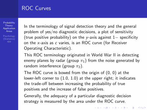
In the terminology of signal detection theory and the generalproblem of yes/no diagnostic decisions, a plot of sensitivity(true positive probability) on the y -axis against 1− specificityon the x-axis as c varies, is an ROC curve (for ReceiverOperating Characteristic).

This ROC terminology originated in World War II in detectingenemy planes by radar (group π1) from the noise generated byrandom interference (group π2).

The ROC curve is bowed from the origin of (0, 0) at thelower-left corner to (1.0, 1.0) at the upper right; it indicatesthe trade-off between increasing the probability of truepositives and the increase of false positives.

Generally, the adequacy of a particular diagnostic decisionstrategy is measured by the area under the ROC curve.

ProbabilityTheory:

ApplicationAreas


484

Probability and Litigation

Jack Weinstein is a sitting federal judge in the Eastern Districtof New York (Brooklyn).

He also may be the only federal judge ever to publish an articlein a major statistics journal (Statistical Science, 1988, 3,286–297, “Litigation and Statistics”).

This last work developed out of Weinstein’s association in themiddle 1980s with the National Academy of Science’s Panel onStatistical Assessment as Evidence in the Courts.

This panel produced the comprehensive Springer-Verlagvolume. The Evolving Role of Statistical Assessments asEvidence in the Courts (1988; Stephen E. Fienberg, Editor).

ProbabilityTheory:

ApplicationAreas


484

290th Commandment

The importance that Weinstein gives to the role of probabilityand statistics in the judicial process is best expressed byWeinstein himself (we quote from his Statistical Sciencearticle):

The use of probability and statistics in the legal process is notunique to our times. Two thousand years ago, Jewish law, asstated in the Talmud, cautioned about the use of probabilisticinference. The medieval Jewish commentator Maimonidessummarized this traditional view in favor of certainty when henoted:

ProbabilityTheory:

ApplicationAreas


484“The 290th Commandment is a prohibition to carry outpunishment on a high probability, even close to certainty . . .No punishment [should] be carried out except where . . . thematter is established in certainty beyond any doubt . . . ”

That view, requiring certainty, is not acceptable to the courts.We deal not with the truth, but with probabilities, in criminalas well as civil cases. Probabilities, express and implied,support every factual decision and inference we make in court.

ProbabilityTheory:

ApplicationAreas


484 Maimonides’ description of the 290th Negative Commandmentis given in its entirety in an appendix.

According to this commandment, an absolute certainty of guiltis guaranteed by having two witnesses to exactly the samecrime.

Such a probability of guilt being identically one is what is meantby the contemporary phrase “without any shadow of a doubt.”

ProbabilityTheory:

ApplicationAreas


484

Two points need to be emphasized about this Mitzvah (Jewishcommandment).

One is the explicit unequalness of costs attached to the falsepositive and negative errors:

“it is preferable that a thousand guilty people be set free thanto execute one innocent person.”

The second is in dealing with what would now be characterizedas the (un)reliability of eyewitness testimony.

Two eyewitnesses are required, neither is allowed to make justan inference about what happened but must have observed itdirectly, and exactly the same crime must be observed by botheyewitnesses.

ProbabilityTheory:

ApplicationAreas


484

Fatico Case

Judge Weinstein’s interest in how probabilities could be part ofa judicial process goes back some years before the NationalResearch Council Panel.

In one relevant opinion from 1978, United States v. Fatico, hewrestled with how subjective probabilities might be related tothe four levels of a “legal burden of proof”; what level wasrequired in this particular case; and, finally, was it then met.

The four (ordered) levels are: preponderance of the evidence;clear and convincing evidence; clear, unequivocal, andconvincing evidence; and proof beyond a reasonable doubt.

The case in point involved proving that Daniel Fatico was a“made” member of the Gambino organized crime family, andthus could be given a “Special Offender” status.

ProbabilityTheory:

ApplicationAreas


484

Other Standards

Other common standards used for police searches or arrestsmight also be related to an explicit probability scale.

The lowest standard (perhaps a probability of 20%) would be“reasonable suspicion” to determine whether a briefinvestigative stop or search by any governmental agent iswarranted (in the 2010 “Papers, Please” law in Arizona, a“reasonable suspicion” standard is set for requestingdocumentation).

A higher standard would be “probable cause” to assess whethera search or arrest is warranted, or whether a grand jury shouldissue an indictment.

A value of, say, 40% might indicate a “probable cause” levelthat would put it somewhat below a “preponderance of theevidence” criterion.

ProbabilityTheory:

ApplicationAreas


484

Probability of Causation

Judge Weinstein is best known for the mass (toxic) tort caseshe has presided over for the last four decades (for example,asbestos, breast implants, Agent Orange).

In all of these kinds of torts, there is a need to establish, in alegally acceptable fashion, some notion of causation.

There is first a concept of general causation concerned withwhether an agent can increase the incidence of disease in agroup;

because of individual variation, a toxic agent will not generallycause disease in every exposed individual.

Specific causation deals with an individual’s disease beingattributable to exposure from an agent.

ProbabilityTheory:

ApplicationAreas


484

Cohort Studies

The establishment of general causation (and a necessaryrequirement for establishing specific causation) typically relieson a cohort study.

Disease No Disease Row Sums

Exposed N11 N12 N1+

Not Exposed N21 N22 N2+

ProbabilityTheory:

ApplicationAreas


484

Here, N11, N12, N21, and N22 are the cell frequencies; N1+ andN2+ are the row frequencies.

Conceptually, these data are considered generated from two(statistically independent) binomial distributions for the“Exposed” and “Not Exposed” conditions.

If we let pE and pNE denote the two underlying probabilities ofgetting the disease for particular cases within the conditions,respectively, the ratio pE

pNEis referred to as the relative risk

(RR), and may be estimated with the data as follows:

ProbabilityTheory:

ApplicationAreas


484

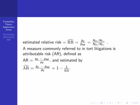
estimated relative risk = RR = pEpNE

= N11/N1+

N21/N2+.

A measure commonly referred to in tort litigations isattributable risk (AR), defined as

AR = pE − pNEpE

, and estimated by

AR = pE − pNEpE

= 1− 1

RR.

ProbabilityTheory:

ApplicationAreas


484

Attributable Risk

Attributable risk, also known as the “attributable proportion ofrisk” or the “etiologic fraction,” represents the amount ofdisease among exposed individuals assignable to the exposure.

It measures the maximum proportion of the disease attributableto exposure from an agent, and consequently, the maximumproportion of disease that could be potentially prevented byblocking the exposure’s effect or eliminating the exposure itself.

If the association is causal, AR is the proportion of disease inan exposed population that might be caused by the agent, andtherefore, that might be prevented by eliminating exposure tothe agent.

ProbabilityTheory:

ApplicationAreas


484

The common legal standard used to argue for both specific andgeneral causation is an RR of 2.0, or an AR of 50%.

At this level, it is “as likely as not” that exposure “caused” thedisease (or “as likely to be true as not,” or “the balance of theprobabilities”).

Obviously, one can never be absolutely certain that a particularagent was “the” cause of a disease in any particular individual,but to allow an idea of “probabilistic causation” or“attributable risk” to enter into legal arguments provides ajustifiable basis for compensation.

It has now become routine to do this in the courts.

ProbabilityTheory:

ApplicationAreas


484

Probability Scales and Rulers

The topic of relating a legal understanding of burdens of proofto numerical probability values has been around for a very longtime.

Fienberg (1988) provides a short discussion of JeremyBentham’s (1827) suggestion of a “persuasion thermometer,”and some contemporary reaction to this idea from ThomasStarkie (1833):

Jeremy Bentham appears to have been the first jurist toseriously propose that witnesses and judges numericallyestimate their degrees of persuasion. Bentham envisioned akind of moral thermometer:

The scale being understood to be composed of ten degrees—inthe language applied by the French philosophers tothermometers, a decigrade scale—a man says, My persuasion isat 10 or 9, etc. affirmative, or at least 10, etc. negative . . .

ProbabilityTheory:

ApplicationAreas


484

Several particularly knotty problems and (mis)interpretationswhen it comes to assigning numbers to the possibility of guiltarise most markedly in eyewitness identification.

Because cases involving eyewitness testimony are typicallycriminal cases, they demand burdens of proof “beyond areasonable doubt”;

thus, the (un)reliability of eyewitness identification becomesproblematic when it is the primary (or only) evidence presentedto meet this standard.

ProbabilityTheory:

ApplicationAreas


484

As discussed extensively in the judgment and decision-makingliterature, there is a distinction between making a subjectiveestimate of some quantity, and one’s confidence in thatestimate once made.

For example, suppose someone picks a suspect out of a lineup,and is then asked the (Bentham) question,

“on a scale of from one to ten, characterize your level of‘certainty’.”

Does an answer of “seven or eight” translate into a probabilityof innocence of two or three out of ten?

ProbabilityTheory:

ApplicationAreas


484

Exactly such confusing situations, however, arise.

We give a fairly extensive redaction in an appendix of anopinion from the District of Columbia Court of Appeals in acase named “In re As.H” (2004).

It combines extremely well both the issues of eyewitness(un)reliability and the attempt to quantify that which may bebetter left in words;

the dissenting Associate Judge Farrel noted pointedly:

“I believe that the entire effort to quantify the standard ofproof beyond a reasonable doubt is a search for fool’s gold.”

ProbabilityTheory:

ApplicationAreas


484

Betting, Gaming, and Risk

Antoine Gombaud, better known as the Chevalier de Mere, wasa French writer and amateur mathematician from the early17th century.

He is important to the development of probability theorybecause of one specific thing; he asked a mathematician, BlaisePascal, about a gambling problem dating from the MiddleAges, named “the problem of points.”

The question was one of fairly dividing the stakes amongindividuals who had agreed to play a certain number of games,but for whatever reason had to stop before they were finished.

Pascal in a series of letters with Pierre de Fermat, solved thisequitable division task, and in the process laid out thefoundations for a modern theory of probability.

ProbabilityTheory:

ApplicationAreas


484

Pascal and Fermat also provided the Chevalier with a solutionto a vexing problem he was having in his own personalgambling.

Apparently, the Chevalier had been very successful in makingeven money bets that a six would be rolled at least once in fourthrows of a single die.

But when he tried a similar bet based on tossing two dice 24times and looking for a double-six to occur, he was singularlyunsuccessful in making any money.

The reason for this difference between the Chevalier’s twowagers was clarified by the formalization developed by Pascaland Fermat for such games of chance.

ProbabilityTheory:

ApplicationAreas


484

Some Useful Concepts

A simple experiment is some process that we engage in thatleads to one single outcome from a set of possible outcomesthat could occur.

For example, a simple experiment could consist of rolling asingle die once, where the set of possible outcomes is{1, 2, 3, 4, 5, 6} (note that curly braces will be used consistentlyto denote a set).

Or, two dice could be tossed and the number of spotsoccurring on each die noted; here, the possible outcomes areinteger number pairs: {(a, b) | 1 ≤ a ≤ 6; 1 ≤ b ≤ 6}.

ProbabilityTheory:

ApplicationAreas


484 Flipping a single coin would give the set of outcomes, {H,T},with “H” for “heads” and “T ” for “tails”;

picking a card from a normal deck could give a set of outcomescontaining 52 objects, or if we were only interested in theparticular suit for a card chosen, the possible outcomes couldbe {H,D,C ,S}, corresponding to heart, diamond, club, andspade, respectively.

ProbabilityTheory:

ApplicationAreas


484

The set of possible outcomes for a simple experiment is thesample space (which we denote by the script letter S).

An object in a sample space is a sample point.

An event is defined as a subset of the sample space, and anevent containing just a single sample point is an elementaryevent.

A particular event is said to occur when the outcome of thesimple experiment is a sample point belonging to the definingsubset for that event.

ProbabilityTheory:

ApplicationAreas


484 As a simple example, consider the toss of a single die, where S= {1, 2, 3, 4, 5, 6}.The event of obtaining an even number is the subset {2, 4, 6};the event of obtaining an odd number is {1, 3, 5};the (elementary) event of tossing a 5 is a subset with a singlesample point, {5}, and so on.

ProbabilityTheory:

ApplicationAreas


484

For a sample space containing K sample points, there are 2K

possible events (that is, there are 2K possible subsets of thesample space).

This includes the “impossible event” (usually denoted by ∅),characterized as that subset of S containing no sample pointsand which therefore can never occur;

and the “sure event,” defined as that subset of S containing allsample points (that is, S itself), which therefore must alwaysoccur.

In our single die example, there are 26

= 64 possible events,including ∅ and S.

ProbabilityTheory:

ApplicationAreas


484

The motivation for introducing the idea of a simple experimentand sundry concepts is to use this structure as an intuitivelyreasonable mechanism for assigning probabilities to theoccurrence of events.

These probabilities are usually assigned through an assumptionthat sample points are equally likely to occur, assuming wehave characterized appropriately what is to be in S.

Generally, only the probabilities are needed for the Kelementary events containing single sample points.

The probability for any other event is merely the sum of theprobabilities for all those elementary events defined by thesample points making up that particular event.

ProbabilityTheory:

ApplicationAreas


484 This last fact is due to the disjoint set property of probabilityintroduced at the beginning of the last chapter.

In the specific instance in which the sample points are equallylikely to occur, the probability assigned to any event is merelythe number of sample points defining the event divided by K .

As special cases, we obtain a probability of 0 for the impossibleevent, and 1 for the sure event.

ProbabilityTheory:

ApplicationAreas


484

The Chevalier Games

One particularly helpful use of the sample space/event conceptsis when a simple experiment is carried out multiple times (for,say, N replications), and the outcomes defining the samplespace are the ordered N-tuples formed from the resultsobtained for the individual simple experiments.

The Chevalier who rolls a single die four times, generates thesample space

{(D1,D2,D3,D4) | 1 ≤ Di ≤ 6, 1 ≤ i ≤ 4} ,that is, all 4-tuples containing the integers from 1 to 6.

Generally, in a replicated simple experiment with K possibleoutcomes on each trial, the number of different N-tuples is KN

(using a well-known arithmetic multiplication rule).

Thus, for the Chevalier example, there are 64 = 1296 possible4-tuples, and each such 4-tuple should be equally likely tooccur (given the “fairness” of the die being used).

ProbabilityTheory:

ApplicationAreas


484

To define the event of “no sixes rolled in four replications,” wewould use the subset (event)

{(D1,D2,D3,D4) | 1 ≤ Di ≤ 5, 1 ≤ i ≤ 4} ,

containing 54 = 625 sample points.

Thus, the probability of “no sixes rolled in four replications” is625/1296 = .4822.

As we will see formally below, the fact that this latterprobability is strictly less than 1/2 gives the Chevalier a distinctadvantage in playing an even money game defined by his beingable to roll at least one six in four tosses of a die.

ProbabilityTheory:

ApplicationAreas


484

The other game that was not as successful for the Chevalier,was tossing two dice 24 times and betting on obtaining adouble-six somewhere in the sequence.

The sample space here is{(P1,P2, . . . ,P24)}, wherePi = {(ai , bi ) | 1 ≤ ai ≤ 6; 1 ≤ bi ≤ 6},and has 3624 possible sample points.

The event of “not obtaining a double-six somewhere in thesequence” would look like the sample space just defined exceptthat the (6, 6) pair would be excluded from each Pi .

ProbabilityTheory:

ApplicationAreas


484

Thus, there are 3524 members in this event.

The probability of “not obtaining a double-six somewhere inthe sequence” is

3524

3624= (

35

36)24 = .5086 .

Because this latter value is greater than 1/2 (in contrast to theprevious gamble), the Chevalier would now be at adisadvantage making an even money bet.

ProbabilityTheory:

ApplicationAreas


484

Random Variables to Evaluate Bets

The best way to evaluate the perils or benefits present in awager is through the device of a discrete random variable.

Suppose X denotes the outcome of some bet; and leta1, . . . , aT represent the T possible payoffs from one wager,where positive values reflect gain and negative values reflectloss.

In addition, we know the probability distribution for X ; that is,P(X = at) for 1 ≤ t ≤ T .

What one expects to realize from one observation on X (orfrom one play of the game) is its expected value,

E (X ) =T∑t=1

atP(X = at).

ProbabilityTheory:

ApplicationAreas


484 If E (X ) is negative, we would expect to lose this much on eachbet; if positive, this is the expected gain on each bet.

When E (X ) is 0, the term “fair game” is applied to thegamble, implying that one neither expects to win or loseanything on each trial; one expects to “break even.”

When E (X ) 6= 0, the game is “unfair” but it could be unfair inyour favor (E (X ) > 0), or unfair against you (E (X ) < 0).

ProbabilityTheory:

ApplicationAreas


484

To evaluate the Chevalier’s two games, suppose X takes on thevalues of +1 and −1 (the winning or losing of one dollar, say).

For the single die rolled four times,E (X ) = (+1)(.5178) + (−1)(.4822) = .0356 ≈ .04.

Thus, the game is unfair in the Chevalier’s favor because heexpects to win a little less than four cents on each wager.

For the 24 tosses of two dice,E (X ) = (+1)(.4914) + (−1)(.5086) = −.0172 ≈ −.02.

Here, the Chevalier is at a disadvantage.

The game is unfair against him, and he expects to lose abouttwo cents on each play of the game.

ProbabilityTheory:

ApplicationAreas


484

Spread Betting

The type of wagering that occurs in roulette or craps is oftenreferred to as fixed-odds betting; you know your chances ofwinning when you place your bet.

A different type of wager is spread betting, invented by amathematics teacher from Connecticut, Charles McNeil, whobecame a Chicago bookmaker in the 1940s.

Here, a payoff is based on the wager’s accuracy; it is no longera simple “win or lose” situation.

Generally, a spread is a range of outcomes, and the bet itself ison whether the outcome will be above or below the spread.

ProbabilityTheory:

ApplicationAreas


484

In common sports betting (for example, NCAA collegebasketball), a “point spread” for some contest is typicallyadvertised by a bookmaker.

If the gambler chooses to bet on the “underdog,” he is said to“take the points” and will win if the underdog’s score plus thepoint spread is greater than that of the favored team;

conversely, if the gambler bets on the favorite, he “gives thepoints” and wins only if the favorite’s score minus the pointspread is greater than the underdog’s score.

In general, the announcement of a point spread is an attemptto even out the market for the bookmaker, and to generate anequal amount of money bet on each side.

The commission that a bookmaker charges will ensure alivelihood, and thus, the bookmaker can be unconcerned aboutthe actual outcome.

ProbabilityTheory:

ApplicationAreas


484

Parimutuel Betting

The term parimutuel betting (based on the French for “mutualbetting”) characterizes the type of wagering system used inhorse racing, dog tracks, jai alai, and similar contests where theparticipants end up in a rank order.

It was devised in 1867 by Joseph Oller, a Catalan impresario(he was also a bookmaker and founder of the Paris MoulinRouge in 1889).

Very simply, all bets of a particular type are first pooledtogether;

the house then takes its commission and the taxes it has to payfrom this aggregate;

finally, the payoff odds are calculated by sharing the residualpool among the winning bets.

ProbabilityTheory:

ApplicationAreas


484

To explain using some notation, suppose there are Tcontestants and bets are made of W1,W2, . . . ,WT on anoutright “win.”

The total pool is Tpool =∑T

t=1 Wt .

If the commission and tax rate is a proportion, R, the residualpool, Rpool , to be allocated among the winning bettors isRpool = Tpool(1− R).

If the winner is denoted by t∗, and the money bet on the winneris Wt∗, the payoff per dollar for a successful bet is Rpool/Wt∗.

We refer to the odds on outcome t∗ as

(Rpool

Wt∗− 1) to 1 .

For example, ifRpool

Wt∗had a value of 9.0, the odds would be 8 to

1: you get 8 dollars back for every dollar bet plus the originaldollar.

ProbabilityTheory:

ApplicationAreas


484

In comparison with casino gambling, parimutuel betting pitsone gambler against other gamblers, and not against the house.

Also, the odds are not fixed but calculated only after thebetting pools have closed (thus, odds cannot be turned intoreal probabilities legitimately; they are empirically generatedbased on the amounts of money bet).

A skilled horse player (or “handicapper”) can make a steadyincome, particularly in the newer Internet “rebate” shops thatreturn to the bettor some percentage of every bet made.

Because of lower overhead, these latter Internet gamingconcerns can reduce their “take” considerably (from, say, 15%to 2%), making a good handicapper an even better living thanbefore.

ProbabilityTheory:

ApplicationAreas


484

Psychological Considerations in Gambling

As shown in the work of Tversky and Kahneman, thepsychology of choice is dictated to a great extent by theframing of a decision problem;

that is, the context into which a particular decision problem isplaced.

The power of framing in how decision situations are assessed,can be illustrated well though an example and the associateddiscussion provided by Tversky and Kahneman (1981, p. 453)and given in the text.

ProbabilityTheory:

ApplicationAreas


484

The Value of Information

The most relevant aspect of any decision-making propositioninvolving risky alternatives is the information one has, both onthe probabilities that might be associated with the gambles andwhat the payoffs might be.

In the 1987 movie, Wall Street, the character playing GordonGekko states:

“The most valuable commodity I know of is information.”

ProbabilityTheory:

ApplicationAreas


484

Dirty Harry

I know what you’re thinkin’. “Did he fire six shots or onlyfive?” Well, to tell you the truth, in all this excitement I kindof lost track myself.— Harry Callahan (Dirty Harry)

The movie quotation just given from Dirty Harry illustrates thecrucial importance of who has information and who doesn’t.

At the end of Callahan’s statement to the bank robber as towhether he felt lucky, the bank robber says:

“I gots to know!”

Harry puts the .44 Magnum to the robber’s head and pulls thetrigger; Harry knew that he had fired six shots and not five.

probability theory: application areas -...

Documents