Probability Review

CSE430 – Operating Systems

Overview of Lecture

• Basic probability review

• Important distributions

• Poison Process

• Markov Chains

• Queuing Systems

Basic Probability concepts

Basic Probability concepts and terms

• Basic concepts by example: dice rolling– (Intuitively) coin tossing and dice rolling are Stochastic Processes– The outcome of a dice rolling is an Event– The values of the outcomes can be expressed as a Random

Variable, which assumes a new value with each event.– The likelihood of an event (or instance) of a random variable is

expressed as a real number in [0,1].• Dice: Random variable• instances or values: 1,2,3,4,5,6• Events: Dice=1, Dice=2, Dice=3, Dice=4, Dice=5, Dice=6• Pr{Dice=1}=0.1666• Pr{Dice=2}=0.1666

– The outcome of the dice is independent of any previous rolls (given that the constitution of the dice is not altered)

Conditional Probabilities

• The likelihood of an event can change if the knowledge and occurrence of another event exists.

• Notation:

• Usually we use conditional probabilities like this:

0}Pr{,}Pr{

}Pr{}|Pr{

B

B

BABA

i

ii BBAA }Pr{}|Pr{}Pr{

Conditional Probability Example• Problem statement (Dice picking):

– There are 3 identical sacks with colored dice. Sack A has 1 red and 4 green dice, sack B has 2 red and 3 green dice and sack C has 3 red and 2 green dice. We choose 1 sack randomly and pull a dice while blind-folded. What is the probability that we chose a red dice?

• Thinking:– If we pick sack A, there is 0.2 probability that we get a red dice– If we pick sack B, there is 0.4 probability that we get a red dice– If we pick sack C, there is 0.6 probability that we get a red dice– For each sack, there is 0.333 probability that we choose that sack

• Result ( R stands for “picking red”):

4.0333.0*6.0333.0*4.0333.02.0

}Pr{}|Pr{}Pr{}|Pr{}Pr{}|Pr{}Pr{

CCRBBRAARR

Probability Distributions

Geometric Distribution

• Expresses the probability of number of trials needed to obtain the event A.– Example: what is the probability that we need k dice

rolls in order to obtain a 6?

• Formula: (for the dice example, p=1/6)

1)1(}Pr{ kppkY

Binomial Distribution

• Expresses the probability of some events occurring out of a larger set of events– Example: we roll the dice n times. What is the

probability that we get k 6’s?

• Formula: (for the dice example, p=1/6)

knk ppknk

nkY

)1(

)!(!

!}Pr{

Solve this Problem

• We roll a regular dice and we toss a coin as many times as the roll indicates.

– What is the probability that we get no tails?

– What is the probability that we get 3 heads?

• Using the same process, we are asked to get 6 tails in total. If we don’t get 6 tails with the first roll, we roll again and repeat as needed. What is the probability that we need more than 1 rolls to get 6 tails?

Continuous Distributions

• Continuous Distributions have:– Probability Density function

– Distribution function:

x

X duufxFxX )()(}Pr{

1)(such that,:)(

dxxfxf XX

Continuous Distributions

• Normal Distribution:

• Uniform Distribution:

• Exponential Distribution:

2

2

2

)(2

2

1),;(

x

ex

elsewhere0

,1

)(bxa

abxfU

00

0);(

t

tetf

t

E

Poisson Process

• It expresses the number of events in a period of time given the rate of occurrence.

• Formula

• A Poisson process with parameter has expected value and variance .

• The time intervals between two events of a Poisson process have an exponential distribution (with mean 1/).

!

)()(

m

ettP

tm

m

Poisson dist. example problem

• An interrupt service unit takes to sec to service an interrupt before it can accept a new one. Interrupt arrivals follow a Poisson process with an average of interrupts/sec.

• What is the probability that an interrupt is lost?– An interrupt is lost if 2 or more interrupts arrive within

a period of to sec.

o

oot

o

to

to

oo

etetet

tPtPY

)1(1!1

)(

!0

)(1

)()(1}2Pr{1}2YPr{

10

10

Markov Chains

The Markov Process

• Discrete time Markov Chain: is a process that changes states at discrete times (steps). Each change in the state is an event.

• The probability of the next state depends solely on the current state, and not on any of the past states: Pr{Xn+1=j|Xo=io, X1=i1, …, Xn=in} = Pr{Xn+1=j| Xn=in}

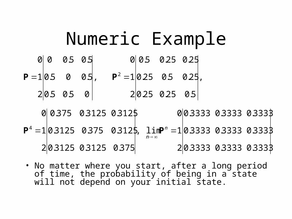
Numeric Example

• No matter where you start, after a long period of time, the probability of being in a state will not depend on your initial state.

3333.03333.03333.0

3333.03333.03333.0

3333.03333.03333.0

2

1

0

lim,

375.03125.03125.0

3125.0375.03125.0

3125.03125.0375.0

2

1

0

,

5.025.025.0

25.05.025.0

25.025.05.0

2

1

0

,

05.05.0

5.005.0

5.05.00

2

1

0

4

2

n

nPP

PP

Example Problem

• A variable bit rate (VBR) audio stream follows a bursty traffic model described by the following two-state Markov chain:

• In the LOW state it has a bit rate of 50Kbps and in the HIGH it has a bit rate of 150Kbps.

• What is the average bit-rate of the stream?

LOW HIGH0.990.01

0.10.9

Example Problem (cont’d)

• We find the stationary probabilities

• Using the stationary probabilities we find the average bitrate:

09.091.0

09.091.0lim,

9.01.0

01.099.0

n

nPP

Kbps5909.015091.050

Queuing Systems

Little’s Law

Little’s Law: Average number of tasks in system =

Average arrival rate x Average response time

Arrivals Departures

System

Queuing System

Queue Server

Queuing System

• What is the system performance?– average number of tasks in server– average number of tasks in queue– average turnaround time in whole system– average waiting time in the queue

Arrival Process

Service Process

Different Queuing Models

• M/M/1

• M/M/m

• M/G/1

• G/M/1

• G/G/1

Results for M/M/1 Queue

• Average number in system = λ/(μ- λ)• Average number in system = λ2/μ(μ- λ)• Average waiting time in system = 1/(μ- λ)• Average waiting time in system = λ/μ(μ- λ)

Queue Server

Queuing System

Poisson Process (rate = λ)

Poisson Process (rate = μ)

Additional Slides

Basic Probability Properties

• The sum of probabilities of all possible values of a random variable is exactly 1.– Pr{Coin=HEADS}+Pr{Coin=TAILS} = 1

• The probability of the union of two events of the same variable is the sum of the separate probabilities of the events– Pr{ Dice=1 Dice=2 } =

Pr{Dice=1}+Pr{Dice=2} = 1/3

Properties of two or more random variables

• The tossing of two or more coins (such that each does not touch any of the other(s) ) simulateously is called (statistically) independent processes (so are the related variables and events).

• The probability of the intersection of two or more independent events is the product of the separate probabilities:– Pr{ Coin1=HEADS Coin2=HEADS } =

Pr{ Coin1=HEADS} Pr{Coin2=HEADS}

Moments and expected values

• mth moment:

• Expected value is the 1st moment: X =E[X]• mth central moment:

• 2nd central moment is called variance (Var[X],X)

i

imi

m xXxXE }Pr{][

i

im

Xim

X xXxXE }Pr{)(])[(

Geometric distribution example

• A wireless network protocol uses a stop-and-wait transmission policy. Each packet has a probability pE of being corrupted or lost.

• What is the probability that the protocol will need 3 transmissions to send a packet successfully?– Solution: 3 transmissions is 2 failures and 1 success, therefore:

• What is the average number of transmissions needed per packet?

2)1(}3Pr{ EE ppY

EEE

i

iEE

i

iEE

i

pppipp

ppiiYiYE

1

1

)1(

1)1()1(

)1(}Pr{][

21

1

1

1

1

Binomial Distribution Example

• Every packet has n bits. There is a probability pΒ that a bit gets corrupted.

• What is the probability that a packet has exactly 1 corrupted bit?

• What is the probability that a packet is not corrupted?

• What is the probability that a packet is corrupted?

111 )1()!1(

!)1(

)!1(!1

!}1Pr{

n

BBn

BB ppn

npp

n

nY

nB

nBB ppp

n

nY )1()1(

)!(!0

!}0Pr{ 0

nBE pYp )1(1}0Pr{1

Transition Matrix

• Putting all the transition probabilities together, we get a transition probability matrix:– The sum of probabilities across each row has to be 1.

1,11

1,10

1,01

1,00

1,1,,1 1

0

}|r{P

nnnn

nnnn

nnnnjinn PP

PP

PiXjX P

Stationary Probabilities

• We denote Pn,n+1 as P(n). If for each step n the transition probability matrix does not change, then we denote all matrices P(n) as P.

• The transition probabilities after 2 steps are given by PP=P2; transition probabilities after 3 steps by P3, etc.

• Usually, limn Pn exists, and shows the probabilities of being in a state after a really long period of time.

• Stationary probabilities are independent of the initial state

Finding the stationary probabilities

0

P

nnnnnn

nn

nn

nnnnnnnnn

nnnnnnnnn

nnnnnnnnn

n

n

n

n

n

n

n

n

n

pxpxpxx

pxpxpxx

pxpxpxx

pxpxpxpxpxpxpxpxpx

pxpxpxpxpxpxpxpxpx

pxpxpxpxpxpxpxpxpx

xxx

xxx

xxx

xxx

xxx

xxx

xxx

xxx

xxx

,,22,11

2,2,222,112

1,1,221,111

,,22,112,2,222,111,1,221,11

,,22,112,2,222,111,1,221,11

,,22,112,2,222,111,1,221,11

21

21

21

21

21

21

21

21

21

Markov Random Walk

• Hitting probability (gambler’s ruin) ui=Pr{XT=0|Xo=i}

• Mean hitting time (soujourn time) vi=E[T|Xo=k]

121

11

21

21

1 isruin sgambler' then if

N

Niii

k

kk u

ppp

qqq

121121121

121

112121

21

11

111

and if

iiN

Ni

iiii

k

kk

v

qqqppp

qqq

Example Problem

• A mouse walks equally likely in the following maze

• Once it reaches room D, it finds food and stays there indefinitely.

• What is the probability that it reaches room D within 5 steps, starting in A?

• Is there a probability it will never reach room D?

A D

Example Problem (cont’d)

1000

1000

1000

1000

lim,

1000

71875.0028125.00

4375.028125.0028125.0

4375.005625.00

,

1000

625.01875.001875.0

4375.0.05625.00

25.0375.00375.0

1000

625.00375.00

25.0375.00375.0

25.0075.00

,

1000

5.025.0025.0

25.0075.00

05.005.0

,

1000

5.005.00

05.005.0

0010

54

32

n

nPPP

PPP

Poisson Distribution

• Poisson Distribution is the limit of Binomial when n and p 0, while the product np is constant. In such a case, assessing or using the probability of a specific event makes little sense, yet it makes sense to use the “rate” of occurrence (λ=np). – Example: if the average number of falling stars

observed every night is λ then what is the probability that we observe k stars fall in a night?

• Formula:

!}Pr{

k

ekY

k

Poisson Distribution Example

• In a bank branch, a rechargeable Bluetooth device sends a “ping” packet to a computer every time a customer enters the door.

• Customers arrive with Poisson distribution of customers per day.

• The Bluetooth device has a battery capacity of m Joules. Every packet takes n Joules, therefore the device can send u=m/n packets before it runs out of battery.

• Assuming that the device starts fully charged in the morning, what is the probability that it runs out of energy by the end of the day?

1

0 !1}Pr{1}Pr{

u

k

k

k

euYuY

Markov Random Walk

• A Random Walk Is a subcase of Markov chains.

• The transition probabilitymatrix looks like this:

1 2 4

1

p

3

rq

p

5

p

qr r 1q

10000

00

00

00

00001

1

2

1

0

111

222

111

NNN qrp

qrp

qrp

N

N

P