probability model based energy efficient and reliable ... · probability model based energy...
TRANSCRIPT

energies
Article
Probability Model Based Energy Efficient andReliable Topology Control Algorithm
Ning Li *, Jose-Fernan Martinez-Ortega, Lourdes Lopez Santidrian andJuan Manuel Meneses Chaus
Research Center on Software Technologies and Multimedia Systems for Sustainability (CITSEM),Universidad Politécnica de Madrid (UPM), Madrid 28031, Spain; [email protected] (J.-F.M.-O.);[email protected] (L.L.S.); [email protected] (J.M.M.C.)* Correspondence: [email protected]; Tel.: +34-688-500-639
Academic Editor: Robert LundmarkReceived: 20 June 2016; Accepted: 12 October 2016; Published: 20 October 2016
Abstract: Topology control is an effective method for improving the performance of wirelesssensor networks (WSNs). Many topology control algorithms can achieve high energy efficiencyby dynamically changing the transmission range of nodes. However, these algorithms prefer tochoose short multihop communication links rather than the long directly communication links whichalso energy efficient probabilistic. Note that these fact, in this paper, we propose a mathematic modelto explore the probability that the long directly communication links are more energy efficient thanthe short links. We investigate the properties of this probability and find out the optimal transmissionrange which has highest probability of energy efficient. Based on this conclusion, we propose theenergy efficient and reliable topology control algorithm (ERTC) to maintain the r-range for the nodesinstead of the k-connection; moreover, ERTC can achieve energy efficient and network connection atthe same time.
Keywords: wireless sensor network (WSN); topology control; energy efficient; reliable
1. Introduction
Wireless sensor networks (WSNs) have become more and more widely used and importantin recent years. The properties of WSNs—which contain hundreds or thousands of sensors—arelimited by the energy, the bandwidth, the capability of computing, etc. Moreover, in most applications,the WSNs are arranged in the remote area where changing the sensor nodes always impossible orinconvenient, so how to save the node energy and prolong the network lifetime is important for WSN.There are many algorithms have been proposed to improve the network reliable and energy efficient forWSN. One remarkable approach is topology control. Topology control has been proposed to addressmany problems in WSNs by adding or deleting nodes/links according to certain algorithms. The aimof topology control is to reduce energy consumption and preserve other fundamental properties forthe network at the same time [1], such as network connectivity, reliability, fault-tolerant, coverage, etc.
In WSNs, topology control can be implemented in three approaches [2]: (1) Power AdjustmentApproach: minimizing the transmission power by adjusting the transmission range of node; in thisapproach, the long distance communication links will be eliminated while the short links will bechosen; (2) Power Model Management: controlling the feature of the operating mode to reduceenergy consumption; there are four operating modes: sleep mode, idle mode, transmission mode,and receiving mode; since the energy consumption during the transmission mode and receivingmode is generally higher than that in the sleep mode [3], so switching the redundant nodes intosleep mode can save energy obviously [4]; (3) Clustering Approach [5]: selecting a set of nodesin the network to construct an efficiently hierarchical topology; the clusterheads are restricted to
Energies 2016, 9, 841; doi:10.3390/en9100841 www.mdpi.com/journal/energies
Energies 2016, 9, 841 2 of 17
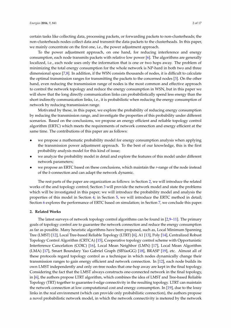
certain tasks like collecting data, processing packets, or forwarding packets to non-clusterheads; thenon-clusterheads nodes collect data and transmit the data packets to the clusterheads. In this paper,we mainly concentrate on the first one, i.e., the power adjustment approach.
To the power adjustment approach, on one hand, for reducing interference and energyconsumption, each node transmits packets with relative low power [6]. The algorithms are generallylocalized, i.e., each node uses only the information that is one or two hops away. The problem ofminimizing the total energy consumption for the whole network is NP-hard in both two and threedimensional space [7,8]. In addition, if the WSN consists thousands of nodes, it is difficult to calculatethe optimal transmission ranges for transmitting the packets to the concerned nodes [3]. On the otherhand, even reducing the transmission range of nodes is the most common and effective approachto control the network topology and reduce the energy consumption in WSN, but in this paper wewill show that the long directly communication links can probabilistically spend less energy than theshort indirectly communication links, i.e., it is probabilistic when reducing the energy consumption ofnetwork by reducing transmission range.
Motivated by these, in this paper, we explore the probability of reducing energy consumptionby reducing the transmission range, and investigate the properties of this probability under differentscenarios. Based on the conclusions, we propose an energy efficient and reliable topology controlalgorithm (ERTC) which meets the requirements of network connection and energy efficient at thesame time. The contributions of this paper are as follows:
• we propose a mathematic probability model for energy consumption analysis when applyingthe transmission power adjustment approach. To the best of our knowledge, this is the firstprobability analysis model for this kind of issue;
• we analyze the probability model in detail and explore the features of this model under differentnetwork parameters;
• we propose an ERTC based on these conclusions, which maintain the r-range of the node insteadof the k-connection and can adapt the network dynamic.
The rest parts of the paper are organization as follows: in Section 2, we will introduce the relatedworks of the and topology control; Section 3 will provide the network model and state the problemswhich will be investigated in this paper; we will introduce the probability model and analysis theproperties of this model in Section 4; in Section 5, we will introduce the ERTC method in detail;Section 6 explores the performance of ERTC based on simulation; in Section 7, we conclude this paper.
2. Related Works
The latest surveys of network topology control algorithms can be found in [2,9–11]. The primarygoals of topology control are to guarantee the network connection and reduce the energy consumptionas far as possible. Many heuristic algorithms have been proposed, such as, Local Minimum SpanningTree (LMST) [12], Local Tree-based Reliable Topology (LTRT) [6], A1 [13], Poly [14], Centralized RobustTopology Control Algorithm (CRTCA) [15], Cooperative topology control scheme with OpportunisticInterference Cancelation (COIC) [16], Local Mean Neighbor (LMN) [17], Local Mean Algorithm(LMA) [17], Smart Boundary Yao Gabriel Graph (SBYaoGG) [18], BRASP [19], etc. Almost all ofthese protocols regard topology control as a technique in which nodes dynamically change theirtransmission ranges to gain energy efficient and network connection. In [12], each node builds itsown LMST independently and only on-tree nodes that one-hop away are kept in the final topology.Considering the fact that the LMST always constructs one-connected network in the final topology,in [6], the authors propose LTRT algorithm, which combines the idea of LMST and Tree-based ReliableTopology (TRT) together to guarantee k-edge connectivity in the resulting topology. LTRT can maintainthe network connection at low computational cost and energy consumption. In [19], due to the lossylinks in the real environment (which can provide only probabilistic connection), the authors proposea novel probabilistic network model, in which the network connectivity is metered by the network

Energies 2016, 9, 841 3 of 17
reachability. The authors explore the minimal transmission power for each node when the networkreachability is above a given threshold. Based on the conclusion, the authors propose BRASP algorithmto improve the energy efficiency and reduce the average node degree. A1 assumes the networktopology as a connected network and finds a set of active nodes to form connected dominating set(CDS) [13]. This algorithm can form a reduced topology while keeping the network connection andcoverage at the same time. In addition, A1 forms the CDS which comprising high energy nodes ina single phase construction process and a set of active nodes for energy efficiency and better sensingcoverage, respectively. Similarly with A1, Poly [14] is also the algorithm based on CDS. In Poly,the network is modeled as a connected graph. The protocol can turn off the unnecessary node andkeep the network connection and coverage at the same time. LMN and LMA are the two typicalpower adjustment topology control algorithms [17]. In LMA, all the nodes can get their node degree.The algorithm sets the minimum threshold and maximum threshold for this number; if the node degreeis less than the minimum threshold, the transmission range will be increased; otherwise, transmissionrange will be reduced. The principle of LMN is similar with LMA, but LMN does not set the maximumand minimum thresholds for the node degree. In LMN, the nodes use the mean neighbors’ nodedegree as the threshold to adjust the transmission ranges.
3. Network Model and Problem Statement
In general, there are three models can express the connection mode between nodes, which areshown in Figure 1 [20]. Figure 1a illustrates the k nearest neighbor model; each node in this model hasconstant node degree and maintains the node degree by changing communication range dynamically.Figure 1b illustrates the disc model; in this model, the transmission range is modeled as a disk withradius r; the nodes connect with other nodes that fall into its communication range. Figure 1c illustratesthe Erdos-Renyi random graph that connects any two nodes by the same probability which is notappropriate in WSNs. Disc model is more plausible in WSN since obtaining k neighbors is not alwaysfeasible due to the communication range limitation [20]. Therefore, in this paper, we only interestedin the Disc model. The nodes in this model are uniform distributed and fixed; moreover, the nodeshave different initial transmission ranges and can change their transmission ranges from zero tothe maximum.
Energies 2016, 9, 841 3 of 17
transmission power for each node when the network reachability is above a given threshold. Based
on the conclusion, the authors propose BRASP algorithm to improve the energy efficiency and
reduce the average node degree. A1 assumes the network topology as a connected network and
finds a set of active nodes to form connected dominating set (CDS) [13]. This algorithm can form a
reduced topology while keeping the network connection and coverage at the same time. In
addition, A1 forms the CDS which comprising high energy nodes in a single phase construction
process and a set of active nodes for energy efficiency and better sensing coverage, respectively.
Similarly with A1, Poly [14] is also the algorithm based on CDS. In Poly, the network is modeled as
a connected graph. The protocol can turn off the unnecessary node and keep the network connection
and coverage at the same time. LMN and LMA are the two typical power adjustment topology
control algorithms [17]. In LMA, all the nodes can get their node degree. The algorithm sets the
minimum threshold and maximum threshold for this number; if the node degree is less than the
minimum threshold, the transmission range will be increased; otherwise, transmission range will be
reduced. The principle of LMN is similar with LMA, but LMN does not set the maximum and
minimum thresholds for the node degree. In LMN, the nodes use the mean neighbors’ node degree
as the threshold to adjust the transmission ranges.
3. Network Model and Problem Statement
In general, there are three models can express the connection mode between nodes, which are
shown in Figure 1 [20]. Figure 1a illustrates the k nearest neighbor model; each node in this model
has constant node degree and maintains the node degree by changing communication range
dynamically. Figure 1b illustrates the disc model; in this model, the transmission range is modeled
as a disk with radius r; the nodes connect with other nodes that fall into its communication range.
Figure 1c illustrates the Erdos-Renyi random graph that connects any two nodes by the same
probability which is not appropriate in WSNs. Disc model is more plausible in WSN since obtaining
k neighbors is not always feasible due to the communication range limitation [20]. Therefore, in this
paper, we only interested in the Disc model. The nodes in this model are uniform distributed and
fixed; moreover, the nodes have different initial transmission ranges and can change their
transmission ranges from zero to the maximum.
1
2
3
4
1
2
3
4
1
2
3
4
pp
p
pp
p
(a) (b) (c)
Figure 1. Different network models: (a) k nearest neighbor model; (b) disc model; and (c)
Erdos-Renyi random graph.
The notations and network definitions used in this paper are as follows:
n The node number of the whole network;
r The Euclidean distance between two nodes u and v, in this paper, we also use r to represent the
initial transmission range;
The distance-power gradient;
uvP The energy required to transmit data from node u to node v;
The probability of energy efficient when applying the power adjustment topology control algorithm.
Figure 1. Different network models: (a) k nearest neighbor model; (b) disc model; and (c) Erdos-Renyirandom graph.
The notations and network definitions used in this paper are as follows:
n The node number of the whole network;r The Euclidean distance between two nodes u and v, in this paper, we also use r to represent the
initial transmission range;γ The distance-power gradient;
Puv The energy required to transmit data from node u to node v;ρ The probability of energy efficient when applying the power adjustment topology control algorithm.
Energies 2016, 9, 841 4 of 17
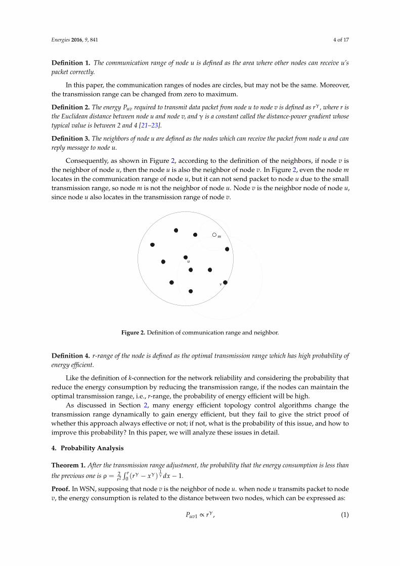
Definition 1. The communication range of node u is defined as the area where other nodes can receive u’spacket correctly.
In this paper, the communication ranges of nodes are circles, but may not be the same. Moreover,the transmission range can be changed from zero to maximum.
Definition 2. The energy Puv required to transmit data packet from node u to node v is defined as rγ, where r isthe Euclidean distance between node u and node v, and γ is a constant called the distance-power gradient whosetypical value is between 2 and 4 [21–23].
Definition 3. The neighbors of node u are defined as the nodes which can receive the packet from node u and canreply message to node u.
Consequently, as shown in Figure 2, according to the definition of the neighbors, if node v isthe neighbor of node u, then the node u is also the neighbor of node v. In Figure 2, even the node mlocates in the communication range of node u, but it can not send packet to node u due to the smalltransmission range, so node m is not the neighbor of node u. Node v is the neighbor node of node u,since node u also locates in the transmission range of node v.
Energies 2016, 9, 841 4 of 17
Definition 1. The communication range of node u is defined as the area where other nodes can receive u’s
packet correctly.
In this paper, the communication ranges of nodes are circles, but may not be the same.
Moreover, the transmission range can be changed from zero to maximum.
Definition 2. The energy uvP required to transmit data packet from node u to node v is defined as r , where
r is the Euclidean distance between node u and node v, and γ is a constant called the distance-power gradient
whose typical value is between 2 and 4 [21–23].
Definition 3. The neighbors of node u are defined as the nodes which can receive the packet from node u and
can reply message to node u.
Consequently, as shown in Figure 2, according to the definition of the neighbors, if node v is
the neighbor of node u, then the node u is also the neighbor of node v. In Figure 2, even the node m
locates in the communication range of node u, but it can not send packet to node u due to the small
transmission range, so node m is not the neighbor of node u. Node v is the neighbor node of node u,
since node u also locates in the transmission range of node v.
m
u
v
Figure 2. Definition of communication range and neighbor.
Definition 4. r-range of the node is defined as the optimal transmission range which has high probability of
energy efficient.
Like the definition of k-connection for the network reliability and considering the probability
that reduce the energy consumption by reducing the transmission range, if the nodes can maintain
the optimal transmission range, i.e., r-range, the probability of energy efficient will be high.
As discussed in Section 2, many energy efficient topology control algorithms change the
transmission range dynamically to gain energy efficient, but they fail to give the strict proof of
whether this approach always effective or not; if not, what is the probability of this issue, and how
to improve this probability? In this paper, we will analyze these issues in detail.
4. Probability Analysis
Theorem 1. After the transmission range adjustment, the probability that the energy consumption is less
than the previous one is
1
2 0
2( ) 1
r
r x dxr
.
Proof. In WSN, supposing that node v is the neighbor of node u. when node u transmits packet to
node v, the energy consumption is related to the distance between two nodes, which can be
expressed as:
1uvP r , (1)
Figure 2. Definition of communication range and neighbor.
Definition 4. r-range of the node is defined as the optimal transmission range which has high probability ofenergy efficient.
Like the definition of k-connection for the network reliability and considering the probability thatreduce the energy consumption by reducing the transmission range, if the nodes can maintain theoptimal transmission range, i.e., r-range, the probability of energy efficient will be high.
As discussed in Section 2, many energy efficient topology control algorithms change thetransmission range dynamically to gain energy efficient, but they fail to give the strict proof ofwhether this approach always effective or not; if not, what is the probability of this issue, and how toimprove this probability? In this paper, we will analyze these issues in detail.
4. Probability Analysis
Theorem 1. After the transmission range adjustment, the probability that the energy consumption is less than
the previous one is ρ = 2r2
∫ r0 (r
γ − xγ)1γ dx− 1.
Proof. In WSN, supposing that node v is the neighbor of node u. when node u transmits packet to nodev, the energy consumption is related to the distance between two nodes, which can be expressed as:
Puv1 ∝ rγ, (1)

Energies 2016, 9, 841 5 of 17
where r is the Euclidean distance between node u and node v, γ is the distance-power gradient thatdepending on the characteristics of the communication medium (2 ≤ γ ≤ 4, γ ≥ 2 for outdoorpropagation modes [23]); Puv1 is the power needed for link between node u and node v.
If the transmission ranges of node u and node v are reduced based on the topology controlalgorithm, then node u and node v cannot communicate directly, which is shown in Figure 3.As a result, node n will be chosen as the relay node, where node n is the neighbor of both nodeu and node v. Thus, the energy needed to transmit packets from node u to node v will be:
Puv2 ∝ r1γ + r2
γ, (2)
where r1 is the Euclidean distance between node u and node n, r2 is the Euclidean distance betweennode n and node v; Puv2 is the power needed for communicating between node u and node v by usingrelay node n.
Energies 2016, 9, 841 5 of 17
where r is the Euclidean distance between node u and node v, is the distance-power gradient
that depending on the characteristics of the communication medium ( 2 4 , 2 for outdoor
propagation modes [23]); 1uvP is the power needed for link between node u and node v.
If the transmission ranges of node u and node v are reduced based on the topology control
algorithm, then node u and node v cannot communicate directly, which is shown in Figure 3. As a
result, node n will be chosen as the relay node, where node n is the neighbor of both node u and
node v. Thus, the energy needed to transmit packets from node u to node v will be:
2 1 2uvP r r , (2)
where 1r is the Euclidean distance between node u and node n, 2r is the Euclidean distance
between node n and node v; 2uvP is the power needed for communicating between node u and
node v by using relay node n.
Figure 3. Transmission range adjustment.
Therefore, the issues we need to solve are when 2uvP is smaller than 1uvP and what is the
probability that 2uvP smaller than 1uvP . For exploring these issues, we define the Energy efficient
Dominating Sets (EDS) as follows:
1 2
1 2
1
2
0
0
uv uvP P
r r r
r r
r r
, (3)
where the first constraint means the energy consumption after power adjustment is smaller than the
previous one; the second constraint make sure node u still can communication with node v by using
a relay node; the third and the fourth constraints guarantee the transmission ranges of each nodes
are smaller than the previous. The EDS is shown in Figure 4.
1r
2r
r
rO
A
B
C
1 2r r r
1 2r r r
Figure 4. The Energy efficient Dominating Sets (EDS) shown in Equation (3).
Figure 3. Transmission range adjustment.
Therefore, the issues we need to solve are when Puv2 is smaller than Puv1 and what is the probabilitythat Puv2 smaller than Puv1. For exploring these issues, we define the Energy efficient Dominating Sets(EDS) as follows:
Puv1 ≥ Puv2
r1 + r2 ≥ r0 < r1 ≤ r0 < r2 ≤ r
, (3)
where the first constraint means the energy consumption after power adjustment is smaller than theprevious one; the second constraint make sure node u still can communication with node v by usinga relay node; the third and the fourth constraints guarantee the transmission ranges of each nodes aresmaller than the previous. The EDS is shown in Figure 4.
Energies 2016, 9, 841 5 of 17
where r is the Euclidean distance between node u and node v, is the distance-power gradient
that depending on the characteristics of the communication medium ( 2 4 , 2 for outdoor
propagation modes [23]); 1uvP is the power needed for link between node u and node v.
If the transmission ranges of node u and node v are reduced based on the topology control
algorithm, then node u and node v cannot communicate directly, which is shown in Figure 3. As a
result, node n will be chosen as the relay node, where node n is the neighbor of both node u and
node v. Thus, the energy needed to transmit packets from node u to node v will be:
2 1 2uvP r r , (2)
where 1r is the Euclidean distance between node u and node n, 2r is the Euclidean distance
between node n and node v; 2uvP is the power needed for communicating between node u and
node v by using relay node n.
Figure 3. Transmission range adjustment.
Therefore, the issues we need to solve are when 2uvP is smaller than 1uvP and what is the
probability that 2uvP smaller than 1uvP . For exploring these issues, we define the Energy efficient
Dominating Sets (EDS) as follows:
1 2
1 2
1
2
0
0
uv uvP P
r r r
r r
r r
, (3)
where the first constraint means the energy consumption after power adjustment is smaller than the
previous one; the second constraint make sure node u still can communication with node v by using
a relay node; the third and the fourth constraints guarantee the transmission ranges of each nodes
are smaller than the previous. The EDS is shown in Figure 4.
1r
2r
r
rO
A
B
C
1 2r r r
1 2r r r
Figure 4. The Energy efficient Dominating Sets (EDS) shown in Equation (3). Figure 4. The Energy efficient Dominating Sets (EDS) shown in Equation (3).

Energies 2016, 9, 841 6 of 17
According the definition of EDS and the principle of linear programming, the EDS is the shadowarea in Figure 4. The area ABC means the whole values which satisfy the second, third, and fourthconstraints in Equation (3); the area
>AB is the set that the energy consumption is smaller than the
previous. Therefore, the probability that the energy consumption is less than the previous one is theproportion of area
>AB in area ABC, which can be calculated as:
ρ =2r2
∫ r
0(rγ − xγ)
1γ dx− 1, (4)
where x is the transmission range of nodes and 0 < x < r.
Lemma 1. With the increasing of γ (2 ≤ γ ≤ 4), the probability ρ will increase from 0.5708 to 0.8541.
Proof. Considering the first derivative function of ρ on γ:
ρ′γ =d[ 2
r2
∫ r0 (r
γ − xγ)1γ dx− 1]
dγ, (5)
In order to simplify the denotation, we define:
f (γ) = (rγ − xγ)1γ , (6)
Therefore, Equation (5) can be rewritten as:
ρ′γ =d[ 2
r2
∫ r0 f (γ)dx− 1]
dγ, (7)
Since 0 < x < r, so if we can prove f (γ) is an increasing function, then we can conclude that ρ(γ)is also the increasing function with γ. The first derivative function of f (γ) on γ is:
f ′(γ) = e1γ (rγ−xγ) · γ·
1rγ−xγ ·(r
γln(r)−xγlnx)−ln(rγ−xγ)γ2
> e1γ (rγ−xγ) · ln(rγ)−ln(rγ−xγ)
γ2 > 0, (8)
As f ′(γ) > 0, so f (γ) is an increasing function. Thus, the probability ρ will increase with theincreasing of γ. In addition, the maximum and minimum values of ρ are as follows:
ρmin = ρ2 = 0.5708, (9)
ρmax = ρ4 = 0.8541, (10)
This can also be found in Figure 5.As shown in Figure 5, with the increasing of γ, the probability ρ increases. The maximum value of
ρ is 0.8741 and the minimum value is only 0.5708. This demonstrates that the algorithm which reducesthe energy consumption by adjusting the transmission range is probabilistic, i.e., short transmissionrange does not mean small energy consumption. The reason why the probability increases with theincreasing of γ is that with the increasing of γ, the energy consumption is more and more seriouslyeffected by the distance between two nodes, which can be concluded from Equation (1); so if thetransmission range changes, the energy consumption will be changed obviously.
Energies 2016, 9, 841 7 of 17Energies 2016, 9, 841 7 of 17
2 2.2 2.4 2.6 2.8 3 3.2 3.4 3.6 3.8 40.55
0.6
0.65
0.7
0.75
0.8
0.85
0.9
0.95
distance-power gradient (γ)
Pro
babili
ty (
ρ)
Figure 5. The relationship between γ and ρ .
Lemma 2. With constant γ , the probability ρ will keep constant with the variation of the initial
transmission range r.
Proof. We can prove this conclusion by simulation. The result can be found in Figure 6.
0 0.1 0.2 0.3 0.4 0.5 0.6 0.7 0.8 0.9 10.55
0.6
0.65
0.7
0.75
0.8
0.85
0.9
0.95
Transmission range (r)
Pro
babili
ty (
ρ)
γ=2
γ=3
γ=4
Figure 6. Relationship between r and ρ for γ .
Figure 6 illustrates that with the increasing of r, the probability ρ will keep constant. In
addition, when γ increases, the probability increases, too; and the bigger the γ , the small
increasing rate is, which is consistent with the conclusion of Lemma 1 (shown in Figure 5).
The Lemma 2 indicates that the probability is nothing to do with the initial transmission range,
i.e., no matter what r is, with constant γ , the probability will be the same.
Lemma 3. With fixed value of γ , when the transmission range is 1/γ(1/ 2) r , the probability ρe can get the
maximum value.
Proof. When applying the power adjustment topology control algorithm, the EDS of 1r and 2r are
shown in Equation (3) and Figure 4. Thus, similar with the definition of EDS, the Un-EDS of 1r and
2r can be shown as follows:
1 2
1 2
1
2
0
0
uv uvP P
r r r
r r
r r
, (11)
Figure 5. The relationship between γ and ρ.
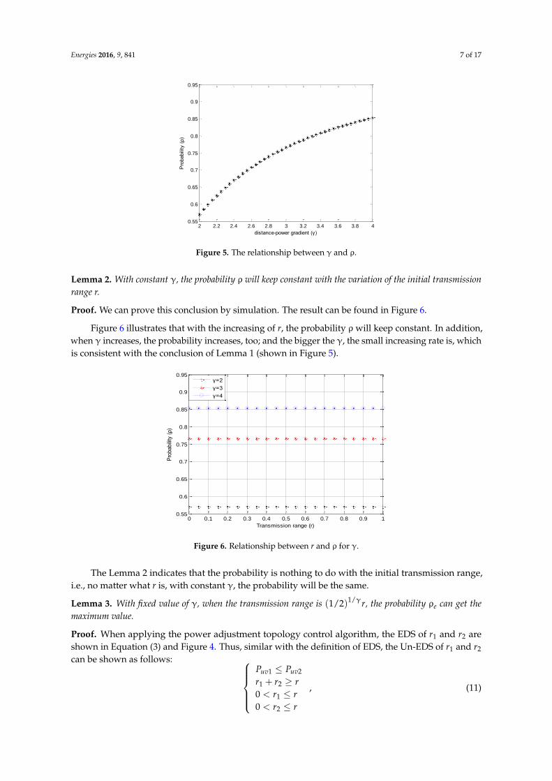
Lemma 2. With constant γ, the probability ρ will keep constant with the variation of the initial transmissionrange r.
Proof. We can prove this conclusion by simulation. The result can be found in Figure 6.
Figure 6 illustrates that with the increasing of r, the probability ρ will keep constant. In addition,when γ increases, the probability increases, too; and the bigger the γ, the small increasing rate is, whichis consistent with the conclusion of Lemma 1 (shown in Figure 5).
Energies 2016, 9, 841 7 of 17
2 2.2 2.4 2.6 2.8 3 3.2 3.4 3.6 3.8 40.55
0.6
0.65
0.7
0.75
0.8
0.85
0.9
0.95
distance-power gradient (γ)
Pro
babili
ty (
ρ)
Figure 5. The relationship between γ and ρ .
Lemma 2. With constant γ , the probability ρ will keep constant with the variation of the initial
transmission range r.
Proof. We can prove this conclusion by simulation. The result can be found in Figure 6.
0 0.1 0.2 0.3 0.4 0.5 0.6 0.7 0.8 0.9 10.55
0.6
0.65
0.7
0.75
0.8
0.85
0.9
0.95
Transmission range (r)
Pro
babili
ty (
ρ)
γ=2
γ=3
γ=4
Figure 6. Relationship between r and ρ for γ .
Figure 6 illustrates that with the increasing of r, the probability ρ will keep constant. In
addition, when γ increases, the probability increases, too; and the bigger the γ , the small
increasing rate is, which is consistent with the conclusion of Lemma 1 (shown in Figure 5).
The Lemma 2 indicates that the probability is nothing to do with the initial transmission range,
i.e., no matter what r is, with constant γ , the probability will be the same.
Lemma 3. With fixed value of γ , when the transmission range is 1/γ(1/ 2) r , the probability ρe can get the
maximum value.
Proof. When applying the power adjustment topology control algorithm, the EDS of 1r and 2r are
shown in Equation (3) and Figure 4. Thus, similar with the definition of EDS, the Un-EDS of 1r and
2r can be shown as follows:
1 2
1 2
1
2
0
0
uv uvP P
r r r
r r
r r
, (11)
Figure 6. Relationship between r and ρ for γ.
The Lemma 2 indicates that the probability is nothing to do with the initial transmission range,i.e., no matter what r is, with constant γ, the probability will be the same.
Lemma 3. With fixed value of γ, when the transmission range is (1/2)1/γr, the probability ρe can get themaximum value.
Proof. When applying the power adjustment topology control algorithm, the EDS of r1 and r2 areshown in Equation (3) and Figure 4. Thus, similar with the definition of EDS, the Un-EDS of r1 and r2
can be shown as follows: Puv1 ≤ Puv2
r1 + r2 ≥ r0 < r1 ≤ r0 < r2 ≤ r
, (11)
Energies 2016, 9, 841 8 of 17
The meanings of each constraint are similar with Equation (3). The values which satisfy Un-EDSmean that the energy consumption of WSN does not decrease after reducing the transmission range.Therefore, how to reduce the size of Un-EDS is an effective method to increase the probability of energyefficient. A possible way is to eliminate some values of r1 and r2 from Un-EDS. Therefore, the newprobability of energy efficient will be:
ρe =
∫ r0 (r
γ − xγ)1γ dx− r2/2
r2/2− (r− r1)(r− r2), (12)
where s = (r− r1)(r− r2) is the eliminated Un-EDS.According the principle of linear programming, when r1 and r2 are in the boundary of Un-EDS,
the eliminated Un-EDS s can get the maximum value, i.e., the probability ρe can get the maximumvalue, which can be found in Equation (12). This means that r1 and r2 should satisfy the constraintas follows:
r2 = (rγ − r1γ)1/γ, (13)
The first derivative function of s and r2 on r1 can be expressed as:
s′r1=
dsdr1
= r2 − r + (r1 − r)r′2r1, (14)
r′2r1=
dr2
dr1= −rγ−1
1 (rγ − rγ1 )1−γγ , (15)
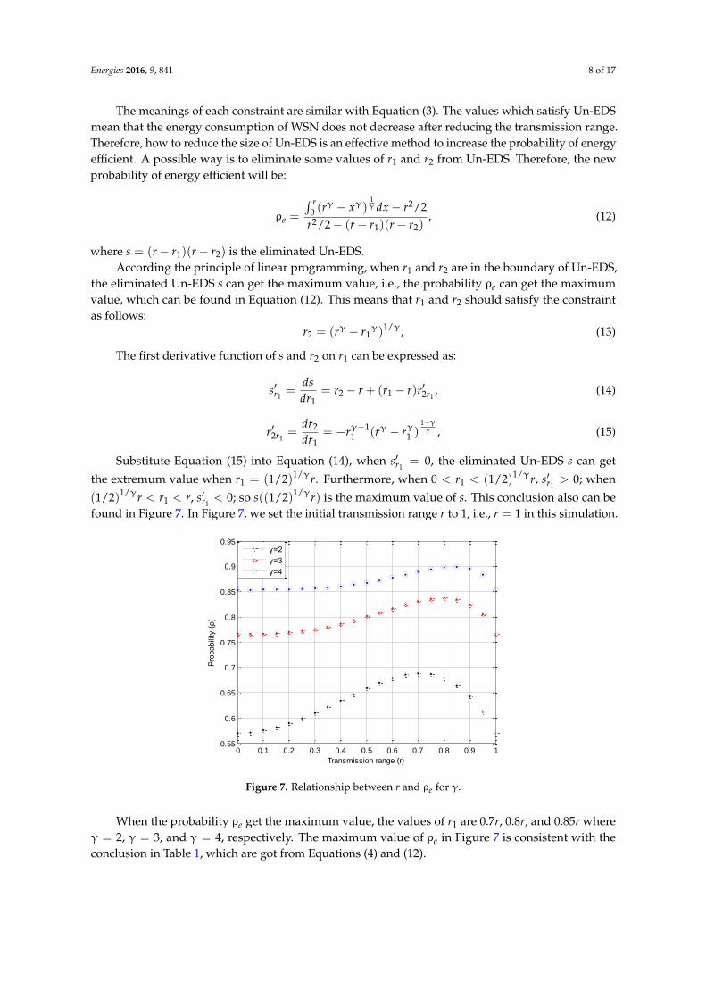
Substitute Equation (15) into Equation (14), when s′r1= 0, the eliminated Un-EDS s can get
the extremum value when r1 = (1/2)1/γr. Furthermore, when 0 < r1 < (1/2)1/γr, s′r1> 0; when
(1/2)1/γr < r1 < r, s′r1< 0; so s((1/2)1/γr) is the maximum value of s. This conclusion also can be
found in Figure 7. In Figure 7, we set the initial transmission range r to 1, i.e., r = 1 in this simulation.
Energies 2016, 9, 841 8 of 17
The meanings of each constraint are similar with Equation (3). The values which satisfy
Un-EDS mean that the energy consumption of WSN does not decrease after reducing the
transmission range. Therefore, how to reduce the size of Un-EDS is an effective method to increase
the probability of energy efficient. A possible way is to eliminate some values of 1r and 2r from
Un-EDS. Therefore, the new probability of energy efficient will be:
1
γ γ 2γ
0
2
1 2
( ) / 2ρ
/ 2 ( )( )
r
e
r x dx r
r r r r r
, (12)
where 1 2( )( )s r r r r is the eliminated Un-EDS.
According the principle of linear programming, when 1r and 2r are in the boundary of
Un-EDS, the eliminated Un-EDS s can get the maximum value, i.e., the probability ρe can get the
maximum value, which can be found in Equation (12). This means that 1r and 2r should satisfy
the constraint as follows:
1/γ
2 1( )r r r , (13)
The first derivative function of s and 2r on 1r can be expressed as:
1 1
' '
2 1 2
1
( )r r
dss r r r r r
dr , (14)
1
1 γ
' 1 γ22 1 1
1
( )r
drr r r r
dr
, (15)
Substitute Equation (15) into Equation (14), when 1
' 0rs , the eliminated Un-EDS s can get the
extremum value when 1/γ
1 (1/ 2)r r . Furthermore, when 1/γ
10 (1/ 2)r r , 1
' 0rs ; when
1/γ
1(1/ 2) r r r , 1
' 0rs ; so 1/γ((1/ 2) )s r is the maximum value of s. This conclusion also can be
found in Figure 7. In Figure 7, we set the initial transmission range r to 1, i.e., 1r in this simulation.
0 0.1 0.2 0.3 0.4 0.5 0.6 0.7 0.8 0.9 10.55
0.6
0.65
0.7
0.75
0.8
0.85
0.9
0.95
Transmission range (r)
Pro
babili
ty (
ρ)
γ=2
γ=3
γ=4
Figure 7. Relationship between r and ρe for γ .
When the probability ρe get the maximum value, the values of 1r are 0.7r, 0.8r, and 0.85r
where γ 2 , γ 3 , and γ 4 , respectively. The maximum value of ρe in Figure 7 is consistent
with the conclusion in Table 1, which are got from Equations (4) and (12).
Figure 7. Relationship between r and ρe for γ.
When the probability ρe get the maximum value, the values of r1 are 0.7r, 0.8r, and 0.85r whereγ = 2, γ = 3, and γ = 4, respectively. The maximum value of ρe in Figure 7 is consistent with theconclusion in Table 1, which are got from Equations (4) and (12).

Energies 2016, 9, 841 9 of 17
Table 1. Probabilities before and after optimizing.
Value of γProbabilities
r1 ρe ρ
γ = 2 0.7071 0.689 0.5708γ = 3 0.7937 0.8379 0.7666γ = 4 0.8409 0.8996 0.8541
From Table 1, we can find that after eliminating some values from the Un-EDS, the probabilities ofenergy efficient increase obviously: 11% when γ = 2, 7% when γ = 3, and 5% when γ = 4. Thus, in thepower adjustment based topology control algorithm, we can use (1/2)1/γr as the optimal transmissionrange of nodes.
5. Energy Efficient and Reliable Topology Control Protocol
In Section 4, we proved that the optimal transmission range for getting high probability of energyefficient is (1/2)1/γr. In this section, we propose an energy efficient and reliable topology controlprotocol based on this conclusion.
In Section 4, we have explored the probability of energy efficient by reducing the transmissionrange in power adjustment based topology control algorithm. For guaranteeing the networkconnection, in this paper, we introduce the conclusions in [24] into our algorithm as the constraints ofnetwork reliable. In [24], the authors prove that when every node connects to its nearest 5.1774lognneighbors, the network is asymptotic connectivity (the asymptotic connectivity means that when thenumber of neighbor nodes is larger than m, then the probability that the network is connected isasymptotic to 1); when each node connects to less than 0.074logn nearest neighbors, the network isasymptotic disconnectivity (the asymptotic disconnectivity means that when the number of neighbornodes is smaller than k, then the probability that the network is disconnected is asymptotic to 1).The simulation result also shows that if the number of neighbors larger than 1.5logn, the probability ofconnectedness increases rapidly to 1 for a modest number of nodes (e.g., n ≈ 30). Therefore, in ERTC,1.5logn will be used as the lower limitation of the neighbors number, i.e., the node degree.
There are two stages in the ERTC: (1) neighbor information collection; (2) transmissionrange adjustment.
5.1. Neighbor Information Collection
In this section, node i broadcast HELLO message mi using initial transmission range ri to calculatethe node degree and the distances to the neighbor nodes. As shown in Section 3, the transmission rangeis a circle, but may not same for each node. The HELLO message mi includes the transmission powerPi, the source node ID Ii, and the version number vsi which is used to decide whether the receivedHELLO message is a new one or not. When the neighbor nodes receive this HELLO message, firstly,comparing the node ID Ii in the HELLO message mi with the node IDs that in the neighbors-list; if thenode ID already exist, then check the version number vsi to find out whether this HELLO message isa new one or not; if not, the HELLO message will be dropped immediately; otherwise, updating theneighbor-list; in case the node ID Ii does not exist in the neighbors-list, then adding the node ID tothe neighbors-list. The distances dij between two nodes are calculated when the node i receives theHELLO message mj from the neighbor nodes by using received signal strength indicator (RSSI) [25,26].When the node i receive the HELLO message mj from other nodes, they will update the neighbors-listbased on the same principle which described above and calculate the node degree N1i.
As shown in Lemma 4, the optimal transmission range for node i is (1/2)1/γri, when the sourcenode i receive the HELLO message mj from the neighbor nodes, it will compare the distance dij with
(1/2)1/γri; the number of neighbor nodes whose distances to the source node i are smaller than(1/2)1/γri will be the node degree of node i with transmission range (1/2)1/γri, which is N2i.

Energies 2016, 9, 841 10 of 17
5.2. Transmission Range Adjustment
In this stage, the node i adjusts their transmission range according the node degree N1i andN2i. As discussed in Section 3, the optimal transmission range for energy efficient is (1/2)1/γri andfor guaranteeing the network connection, the lower limitation of the neighbors number is 1.5logn;therefore, for meeting the requirements of both the energy efficient and the network reliability, thenode degree N1i and N2i should be compared with 1.5logn for deciding the transmission range of nodei. There are three relationships between the node degree and the lower limitation of neighbor numbersin ERTC: (1) N2i ≥ 1.5logn; (2) N2i ≤ 1.5logn ≤ N1i; and (3) N1i ≤ 1.5logn; different relationships willhave different transmission range adjustment strategies:
(i) when N2i ≥ 1.5logn, it means that when the transmission range of node i is (1/2)1/γri, it has thehighest probability to satisfy the requirements of both the energy efficient and network connection.Therefore, the transmission range of node i is reduced to (1/2)1/γri, which is reasonable.
(ii) when N2i ≤ 1.5logn ≤ N1i, this means that when the transmission range of node i is ri, thenetwork connection can be satisfied; however, when the transmission range is (1/2)1/γri, it cannot meet the requirement of network connection. As shown in Figure 7, when the transmissionrange is close to (1/2)1/γri, the probability is close to the highest probability, too. In addition,considering the node in ERTC is uniform distributed, so the node degree ni is proportionalwith the coverage area πr2
i ; therefore, the transmission range in this situation can be set to((1.5logn)/N2i)
1/2 · (1/2)1/γri.(iii) when N1i ≤ 1.5logn, this means the initial transmission range of node i ri can not meet the
requirement of network connection. Therefore, the transmission range should be increased.Similar with the reason in (ii), the transmission range closer to (1/2)1/γri has higher probabilityof energy efficient than that far from (1/2)1/γri and considering the node distribution in ERTC isuniform, so the transmission range in this range can be set to ((1.5logn)/N1i)
1/2 · ri.
The process of the ERTC is:
Energy Efficient and Reliable Topology Control Algorithm (ERTC)1. ERTC:Input:2. The length of the configuration area, Border_length;3. The number of the nodes in the network, n;4. The value of distance-power gradient, γ;Ensure:5. Broadcast the HELLO message mi with initial transmission range ri;6. Receive the HELLO message mj;7. Update the neighbors-list;8. Calculate the node degree N1i;9. Compare the distance between node i and the neighbor nodes with (1/2)1/γri;10. Calculate the node degree N2i;11. if N2i ≥ 1.5logn then
TR = (1/2)1/γri;12. else if N2i ≤ 1.5logn ≤ N1i then
TR = ((1.5logn)/N2i)1/2 · (1/2)1/γri;
13. elseTR = ((1.5logn)/N1i)
1/2 · ri;14. end if15. ri = TR;

Energies 2016, 9, 841 11 of 17
As shown in the table above, the runtime complexity for ERTC is O(n), which is the same as theruntime complexity of LMA and LMN [17]. Therefore, the ERTC can improve the network performancewithout increasing the algorithm complexity seriously.
6. Simulation and Discussion
In this section, we will evaluate the performance of ERTC and discuss the properties in detail.ERTC is power adjustment based topology control algorithm; we compare the performance of
ERTC with LMA and LMN in this paper. The reasons why the LMA and LMN are chosen as thecontrasts are: (1) the ERTC is most similar to LMA and LMN and can be regarded as the extensional ofLMN and LMA based on the theory analysis in Section 4; (2) LMN and LMA are the two typical andbasic power adjustment based topology control algorithms. As a contrast, we use NONE (in whichthere is no topology control algorithm used) as the control group.
The topology control algorithms that will be simulated in this section are as follows.
• NONE: without using topology control algorithm, i.e., forming the network topology randomlyand do not control the network topology artificially.
• LMA: in LMA, there are two node degree thresholds: the minimum threshold and maximumthreshold. If the node degree is smaller than the minimum threshold, the node will increase thetransmission range by certain factor Ainc; otherwise, reducing the transmission ranges by Adec.The nodes in which the node degrees are between the minimum threshold and the maximumthreshold will not change their transmission ranges.
• LMN: in LMN, each node collects the neighbor information from their neighbors, and calculatesthe average neighbors’ node degree. The value will be set as the node degree threshold. If thenode degree is large than this threshold, the transmission range will be reduced; otherwise, it willbe increased.
• ERTC: the algorithm proposed in this paper.
6.1. The Properties of Energy Efficient and Reliable Topology Control Algorithm
In this section, the performance and properties of ERTC will be discussed in detail. We builtthe simulation platform by MATLAB. The simulation parameters are presented as follows: (1) thenode number: 50–200; (2) distribution range: 1 km × 1 km; (3) initial transmission range: 0–200 m;(4) distance-power gradient: γ = 3; (5) simulation time: 3000 s; (6) initial energy supply: 100 J;(7) transmit power: 0–1 mW; (8) receive power: 0.5 mW; (9) transmission rate: 10 kbit/s.
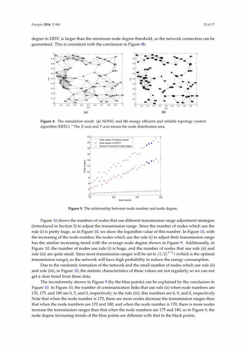
In Figure 8, the network is formed randomly (Figure 8a) and by the ERTC (Figure 8b), respectively.From Figure 8, we can clearly find that the ERTC reduces the number of communication links ofthe original network and guarantees the network connection at the same time. The communicationlinks in Figure 8b are less than that in Figure 8a, which means that after using the ERTC, the energyconsumption will be reduced. The node degree in Figure 8b is obviously smaller than that in Figure 8a;the conclusion can be found in Figure 9, too.
Figure 9 shows the node degree of the original network and the network which uses the ERTC.From Figure 9, we can conclude that with the increasing of the node number, the overall trend ofnode degree is increasing. However, the node degree does not always increase with the rising of thenode number, e.g., as shown in Figure 8, when the node number is 100, 105, 110, and 120, the nodedegree does not keep increasing when the node number rises. The reason is that the network is createdrandomly, so the node degree oscillates near the average node degree; however, the overall trend isincreasing. The increasing trend in ERTC is similar with the original one, but node degrees are smallerthan that. In addition, when the node number is large than 100, the increasing rate of the originalnetwork is faster than that in ERTC. Furthermore, as shown by the blue points in Figure 9, with theincreasing of the node number, the increasing trends are different between the original network andERTC. The reason of this issue will be explained in the next section. Moreover, in Figure 9, the node
Energies 2016, 9, 841 12 of 17
degree in ERTC is larger than the minimum node degree threshold, so the network connection can beguaranteed. This is consistent with the conclusion in Figure 8b.
Energies 2016, 9, 841 12 of 17
0 0.1 0.2 0.3 0.4 0.5 0.6 0.7 0.8 0.9 10
0.1
0.2
0.3
0.4
0.5
0.6
0.7
0.8
0.9
1
1
2
3
4
5
6
7
8
9
10
11
12
13
14
15
16
17
18
19
20
21
22
23
24
25
26
27
2829
30
31
32
3334
35
36
37
38
39
40
41
42
43
4445
46
47
48
49
50
51
52
53
5455
56
57
58
59
60
61
6263
64
65
66
67
68
69
70
71
72
73
74
75
76
77
78
79
80
Km
Km
0 0.1 0.2 0.3 0.4 0.5 0.6 0.7 0.8 0.9 1
0
0.1
0.2
0.3
0.4
0.5
0.6
0.7
0.8
0.9
1
111
22222222222222
333333
4444
555
666666
7777777777
8888888
99999
101010101010
11111111
12121212121212121212121212
131313131313
1414141414
151515151515
161616161616161616161616
17171717171717171717
1818181818181818
191919191919
202020202020
212121212121
222222222222
23232323
2424242424242424242424
252525252525
26262626
27272727
28282828292929
30303030303030
313131313131
32323232323232323232323232
333333333333333434343434343434
3535353535
363636363636363636
3737373737
3838383838
3939393939393939
4040404040
414141
42424242
434343434343
4444444444454545454545454545
4646464646464646464646464646
47474747474747
4848484848484848
494949494949
50505050
51515151515151
5252525252525252525252
5353535353
545454545454555555
56565656
575757575757575757
5858585858585858
59595959595959
6060606060
616161616161
626262626263636363
646464
656565656565656565
6666666666
676767
6868686868686868
696969696969696969
70707070
71717171717171717171
727272727272
737373
74747474747474
7575757575
7676767676
7777777777
7878787878787878
7979797979
8080808080
Km
Km
(a) (b)
Figure 8. The simulation result: (a) NONE; and (b) energy efficient and reliable topology control
algorithm (ERTC). * The X-axis and Y-axis means the node distribution area.
50 100 150 2002
4
6
8
10
12
14
16
18
20
22
Node Number
Node D
egre
e
Node degree of orignial network
Node degree of EERTC
Minimum threshold of node degree
Figure 9. The relationship between node number and node degree.
Figure 9 shows the node degree of the original network and the network which uses the ERTC.
From Figure 9, we can conclude that with the increasing of the node number, the overall trend of
node degree is increasing. However, the node degree does not always increase with the rising of the
node number, e.g., as shown in Figure 8, when the node number is 100, 105, 110, and 120, the node
degree does not keep increasing when the node number rises. The reason is that the network is
created randomly, so the node degree oscillates near the average node degree; however, the overall
trend is increasing. The increasing trend in ERTC is similar with the original one, but node degrees
are smaller than that. In addition, when the node number is large than 100, the increasing rate of the
original network is faster than that in ERTC. Furthermore, as shown by the blue points in Figure 9,
with the increasing of the node number, the increasing trends are different between the original
network and ERTC. The reason of this issue will be explained in the next section. Moreover, in
Figure 9, the node degree in ERTC is larger than the minimum node degree threshold, so the
network connection can be guaranteed. This is consistent with the conclusion in Figure 8b.
Figure 10 shows the numbers of nodes that use different transmission range adjustment
strategies (introduced in Section 5) to adjust the transmission range. Since the number of nodes
which use the rule (i) is pretty huge, so in Figure 10, we show the logarithm value of this number.
In Figure 10, with the increasing of the node number, the nodes which use the rule (i) to adjust their
transmission range has the similar increasing trend with the average node degree shown in Figure
9. Additionally, in Figure 10, the number of nodes use rule (i) is huge, and the number of nodes that
use rule (ii) and rule (iii) are quite small. Since most transmission ranges will be set to 1/γ(1/ 2) r
Figure 8. The simulation result: (a) NONE; and (b) energy efficient and reliable topology controlalgorithm (ERTC). * The X-axis and Y-axis means the node distribution area.
Energies 2016, 9, 841 12 of 17
0 0.1 0.2 0.3 0.4 0.5 0.6 0.7 0.8 0.9 10
0.1
0.2
0.3
0.4
0.5
0.6
0.7
0.8
0.9
1
1
2
3
4
5
6
7
8
9
10
11
12
13
14
15
16
17
18
19
20
21
22
23
24
25
26
27
2829
30
31
32
3334
35
36
37
38
39
40
41
42
43
4445
46
47
48
49
50
51
52
53
5455
56
57
58
59
60
61
6263
64
65
66
67
68
69
70
71
72
73
74
75
76
77
78
79
80
Km
Km
0 0.1 0.2 0.3 0.4 0.5 0.6 0.7 0.8 0.9 1
0
0.1
0.2
0.3
0.4
0.5
0.6
0.7
0.8
0.9
1
111
22222222222222
333333
4444
555
666666
7777777777
8888888
99999
101010101010
11111111
12121212121212121212121212
131313131313
1414141414
151515151515
161616161616161616161616
17171717171717171717
1818181818181818
191919191919
202020202020
212121212121
222222222222
23232323
2424242424242424242424
252525252525
26262626
27272727
28282828292929
30303030303030
313131313131
32323232323232323232323232
333333333333333434343434343434
3535353535
363636363636363636
3737373737
3838383838
3939393939393939
4040404040
414141
42424242
434343434343
4444444444454545454545454545
4646464646464646464646464646
47474747474747
4848484848484848
494949494949
50505050
51515151515151
5252525252525252525252
5353535353
545454545454555555
56565656
575757575757575757
5858585858585858
59595959595959
6060606060
616161616161
626262626263636363
646464
656565656565656565
6666666666
676767
6868686868686868
696969696969696969
70707070
71717171717171717171
727272727272
737373
74747474747474
7575757575
7676767676
7777777777
7878787878787878
7979797979
8080808080
Km
Km
(a) (b)
Figure 8. The simulation result: (a) NONE; and (b) energy efficient and reliable topology control
algorithm (ERTC). * The X-axis and Y-axis means the node distribution area.
50 100 150 2002
4
6
8
10
12
14
16
18
20
22
Node Number
Node D
egre
e
Node degree of orignial network
Node degree of EERTC
Minimum threshold of node degree
Figure 9. The relationship between node number and node degree.
Figure 9 shows the node degree of the original network and the network which uses the ERTC.
From Figure 9, we can conclude that with the increasing of the node number, the overall trend of
node degree is increasing. However, the node degree does not always increase with the rising of the
node number, e.g., as shown in Figure 8, when the node number is 100, 105, 110, and 120, the node
degree does not keep increasing when the node number rises. The reason is that the network is
created randomly, so the node degree oscillates near the average node degree; however, the overall
trend is increasing. The increasing trend in ERTC is similar with the original one, but node degrees
are smaller than that. In addition, when the node number is large than 100, the increasing rate of the
original network is faster than that in ERTC. Furthermore, as shown by the blue points in Figure 9,
with the increasing of the node number, the increasing trends are different between the original
network and ERTC. The reason of this issue will be explained in the next section. Moreover, in
Figure 9, the node degree in ERTC is larger than the minimum node degree threshold, so the
network connection can be guaranteed. This is consistent with the conclusion in Figure 8b.
Figure 10 shows the numbers of nodes that use different transmission range adjustment
strategies (introduced in Section 5) to adjust the transmission range. Since the number of nodes
which use the rule (i) is pretty huge, so in Figure 10, we show the logarithm value of this number.
In Figure 10, with the increasing of the node number, the nodes which use the rule (i) to adjust their
transmission range has the similar increasing trend with the average node degree shown in Figure
9. Additionally, in Figure 10, the number of nodes use rule (i) is huge, and the number of nodes that
use rule (ii) and rule (iii) are quite small. Since most transmission ranges will be set to 1/γ(1/ 2) r
Figure 9. The relationship between node number and node degree.
Figure 10 shows the numbers of nodes that use different transmission range adjustment strategies(introduced in Section 5) to adjust the transmission range. Since the number of nodes which use therule (i) is pretty huge, so in Figure 10, we show the logarithm value of this number. In Figure 10, withthe increasing of the node number, the nodes which use the rule (i) to adjust their transmission rangehas the similar increasing trend with the average node degree shown in Figure 9. Additionally, inFigure 10, the number of nodes use rule (i) is huge, and the number of nodes that use rule (ii) andrule (iii) are quite small. Since most transmission ranges will be set to (1/2)1/γr (which is the optimaltransmission range), so the network will have high probability to reduce the energy consumption.
Due to the randomly formation of the network and the small number of nodes which use rule (ii)and rule (iii), in Figure 10, the statistic characteristics of these values are not regularly, so we can notget a clear trend from these data.
The inconformity shown in Figure 9 (by the blue points) can be explained by the conclusion inFigure 10. In Figure 10, the number of communication links that use rule (ii) when node numbers are170, 175, and 180 are 0, 5, and 0, respectively; to the rule (iii), this numbers are 6, 0, and 0, respectively.Note that when the node number is 175, there are more nodes decrease the transmission ranges thanthat when the node numbers are 170 and 180; and when the node number is 170, there is more nodesincrease the transmission ranges than that when the node numbers are 175 and 180, so in Figure 9, thenode degree increasing trends of the blue points are different with that in the black points.

Energies 2016, 9, 841 13 of 17
Energies 2016, 9, 841 13 of 17
(which is the optimal transmission range), so the network will have high probability to reduce the
energy consumption.
50 100 150 2000
1
2
3
4
5
6
7
8
9
10
Node Number
Diffe
rent
kin
d f
o N
ode N
um
ber
Logarithmic Number of nodes use rule (i)
Number of nodes use rule (ii)
Number of nodes use rule (iii)
Figure 10. The number of different kind of communication links in different scenario.
Due to the randomly formation of the network and the small number of nodes which use rule
(ii) and rule (iii), in Figure 10, the statistic characteristics of these values are not regularly, so we can
not get a clear trend from these data.
The inconformity shown in Figure 9 (by the blue points) can be explained by the conclusion in
Figure 10. In Figure 10, the number of communication links that use rule (ii) when node numbers
are 170, 175, and 180 are 0, 5, and 0, respectively; to the rule (iii), this numbers are 6, 0, and 0,
respectively. Note that when the node number is 175, there are more nodes decrease the
transmission ranges than that when the node numbers are 170 and 180; and when the node number
is 170, there is more nodes increase the transmission ranges than that when the node numbers are
175 and 180, so in Figure 9, the node degree increasing trends of the blue points are different with
that in the black points.
6.2. Compare the Performance of Energy Efficient and Reliabile Topology Control Algorithm with Other
Topology Control Protocols
In this section, the performance of ERTC will be compared with two typical transmission
power adjustment based topology control algorithms: LMA and LMN. The principles of LMA and
LMN have been introduced at the beginning of Section 6.
Figure 11 indicates that the number of communication links in ERTC is the smallest, which can
be found in Figure 11b. In Figure 11c,d, different color lines are used to represent different kinds of
communication links. In Figure 11c, the black links represent the communication links that have
been increased, while the blue lines mean the communication links which have been reduced.
Similarly, in Figure 11d, the black lines indicate that the communication range are not changed, the
red lines mean the communication links are increased, and the blue lines show the communication
links are reduced.
Figure 10. The number of different kind of communication links in different scenario.
6.2. Compare the Performance of Energy Efficient and Reliabile Topology Control Algorithm with OtherTopology Control Protocols
In this section, the performance of ERTC will be compared with two typical transmission poweradjustment based topology control algorithms: LMA and LMN. The principles of LMA and LMN havebeen introduced at the beginning of Section 6.
Figure 11 indicates that the number of communication links in ERTC is the smallest, which canbe found in Figure 11b. In Figure 11c,d, different color lines are used to represent different kinds ofcommunication links. In Figure 11c, the black links represent the communication links that have beenincreased, while the blue lines mean the communication links which have been reduced. Similarly, inFigure 11d, the black lines indicate that the communication range are not changed, the red lines meanthe communication links are increased, and the blue lines show the communication links are reduced.Energies 2016, 9, 841 14 of 17
0 0.1 0.2 0.3 0.4 0.5 0.6 0.7 0.8 0.9 10
0.1
0.2
0.3
0.4
0.5
0.6
0.7
0.8
0.9
1
1
2
3
4
5
67
8
9
10
11
12
13
1415
16
17
18
19
20
21
22
23
24
25
26
27
28
29
30
31
32
33
34
35
36
37
38
39
40
41
42
43
44
45
46 47
48
49
50
51
52
53
54
55
56
57
58
59
60
61
62
63
64
65
66
67
6869
70
71
7273
74
7576
77
78
79
80
Km
Km
0 0.1 0.2 0.3 0.4 0.5 0.6 0.7 0.8 0.9 1
0
0.1
0.2
0.3
0.4
0.5
0.6
0.7
0.8
0.9
1
11111111111
2222222
3333333
4444444444
5555555555
6666667777777
888888
99999999
1010101010101010
1111111111
121212121212
13131313131313
1414141414141414141515151515151515
1616161616161616
1717171717171717171717
1818181818
19191919191919
20202020202020
21212121212121
22222222222222
23232323232323232323
2424242424
2525252525252525
262626262626262626
272727272727
28282828282828
2929292929
303030
31313131313131
3232323232323232
33333333333333
34343434343434
3535353535
363636
37373737373737373737
383838383838383838
3939393939393939
404040404040404040
414141414141
424242424242
4343434343434343
444444444444
454545454545
4646464646464646464646 4747474747474747
48484848484848484848
4949494949494949
505050505050505050
51515151
5252525252525252
53535353535353535353
5454545454545454
555555
56565656
5757575757
5858585858
59595959595959
6060606060606060
61616161616161
626262626262
63636363636363
64646464646464
65656565
666666666666666666
676767
6868686868686869696969
7070707070
717171717171
7272727272727273737373737373
7474747474747474
75757575757575757576767676
7777777777777777
7878787878
79797979797979797979
8080808080808080
Km
Km
(a) (b)
0 0.1 0.2 0.3 0.4 0.5 0.6 0.7 0.8 0.9 10
0.1
0.2
0.3
0.4
0.5
0.6
0.7
0.8
0.9
1
111
222
3333
44
5555555555555555
6666666677
8888
999999999
101010
1111111111
121212121212121212121212
1313
14141515
16161616161616161616
171717171717171717171717171717
1818
191919
202020202020202020202020202020
21212121212121212121212121
2222
232323232323232323232323
2424242424242424
2525252525252525252525
262626262626262626262626
2727272727272727272727
2828282828282828282828
292929292929292929
30303030
313131313131313131
323232323232323232323232323232
333333333333333333
34343434343434343434343434343434
35353535
3636363636363636363636363636363636
37373737373737373737373737
38383838383838383838
3939
404040404040404040404040
4141414141414141414141
42424242424242424242424242424242
43434343
4444444444444444444444444444
454545454545
464646 4747474747474747474747474747
484848
494949
5050505050505050505050
51515151
5252525252
53535353535353535353535353
54545454545454545454
555555555555555555
5656565656
575757
585858
59595959595959595959595959595959595959595959595959
60606060606060606060606060606060
61616161
626262
63636363636363
646464
65656565656565656565
666666
6767676767676767
68686969696969696969
7070707070707070
717171
72727272727272727373
74747474747474747474
757575757575757575757576767676767676
7777
787878787878787878
7979797979797979797979
8080
Km
Km
0 0.1 0.2 0.3 0.4 0.5 0.6 0.7 0.8 0.9 1
0
0.1
0.2
0.3
0.4
0.5
0.6
0.7
0.8
0.9
1
111111111111
222222222
33333333
444444444444
555555555555
66666666677777777777
88888888
999999999
101010101010101010101010
111111111111
1212121212121212
1313131313131313
14141414141414141415151515151515151515151515
16161616161616161616
17171717171717171717171717
1818181818181818
19191919191919191919
20202020202020202020
2121212121212121
22222222222222222222
23232323232323232323232323
242424242424242424
2525252525252525252525
262626262626262626262626
2727272727272727272727
2828282828282828282828
292929292929292929
303030303030303030
313131313131313131
323232323232323232
3333333333333333
343434343434343434
35353535353535
363636363636
37373737373737373737373737
3838383838383838383838
39393939393939393939
404040404040404040404040
41414141414141
4242424242424242
43434343434343434343
44444444444444444444
454545454545
464646464646464646464646 47474747474747474747
48484848484848484848484848
4949494949494949494949
505050505050505050505050
51515151515151
525252525252525252
53535353535353535353535353
54545454545454545454
55555555555555555555
5656565656565656565656
575757575757575757
585858585858585858
5959595959595959595959
60606060606060606060
6161616161616161616161
626262626262626262
6363636363636363
6464646464646464
65656565656565
66666666666666666666
676767676767
6868686868686868686969696969696969
7070707070707070
71717171717171717171
7272727272727272737373737373737373
74747474747474747474
7575757575757575757575757676767676767676
777777777777777777
787878787878
7979797979797979797979
80808080808080808080
Km
Km
(c) (d)
Figure 11. The simulation result: (a) NONE; (b) ERTC; (c) Local Mean Neighbor (LMN); and
(d) Local Mean Algorithm (LMA). * The X-axis and Y-axis means the node distribution area.
Both the LMA and LMN do not take the energy consumption into consideration. Moreover,
since the maximum and minimum thresholds of node degrees in LMA are set by users without
strict definition, the network topology will change greatly under different thresholds. In ERTC, the
node degree thresholds are variation with different network conditions (such as the node numbers,
the different topology, etc.), which aims to maintain r-range instead of k-connection for the nodes.
Furthermore, as shown in Figures 11b and 13, the protocol can meet the requirements of network
connection and energy efficient at the same time in ERTC.
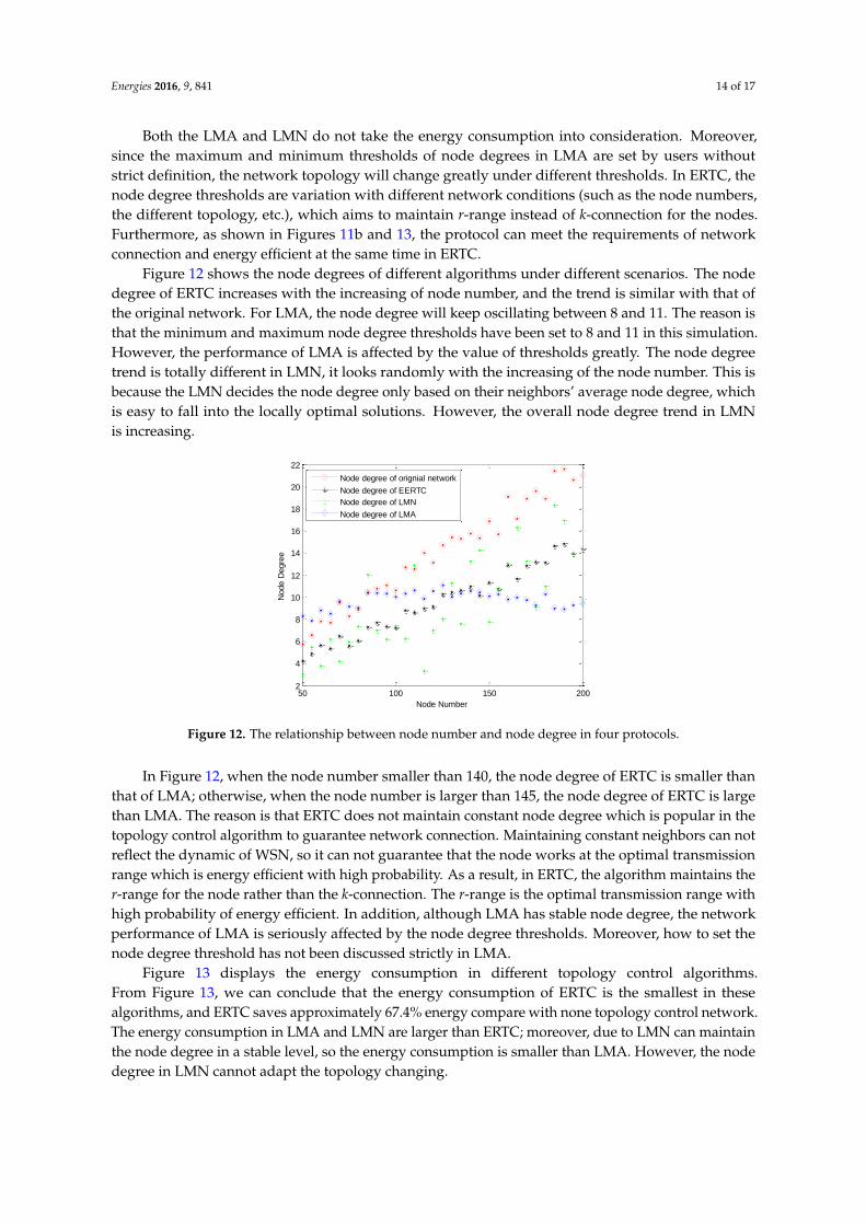
Figure 12 shows the node degrees of different algorithms under different scenarios. The node
degree of ERTC increases with the increasing of node number, and the trend is similar with that of
the original network. For LMA, the node degree will keep oscillating between 8 and 11. The reason
is that the minimum and maximum node degree thresholds have been set to 8 and 11 in this
simulation. However, the performance of LMA is affected by the value of thresholds greatly. The
node degree trend is totally different in LMN, it looks randomly with the increasing of the node
number. This is because the LMN decides the node degree only based on their neighbors’ average
node degree, which is easy to fall into the locally optimal solutions. However, the overall node
degree trend in LMN is increasing.
In Figure 12, when the node number smaller than 140, the node degree of ERTC is smaller than
that of LMA; otherwise, when the node number is larger than 145, the node degree of ERTC is large
than LMA. The reason is that ERTC does not maintain constant node degree which is popular in the
topology control algorithm to guarantee network connection. Maintaining constant neighbors can
not reflect the dynamic of WSN, so it can not guarantee that the node works at the optimal
transmission range which is energy efficient with high probability. As a result, in ERTC, the
algorithm maintains the r-range for the node rather than the k-connection. The r-range is the
optimal transmission range with high probability of energy efficient. In addition, although LMA
Figure 11. The simulation result: (a) NONE; (b) ERTC; (c) Local Mean Neighbor (LMN); and (d) LocalMean Algorithm (LMA). * The X-axis and Y-axis means the node distribution area.
Energies 2016, 9, 841 14 of 17
Both the LMA and LMN do not take the energy consumption into consideration. Moreover,since the maximum and minimum thresholds of node degrees in LMA are set by users withoutstrict definition, the network topology will change greatly under different thresholds. In ERTC, thenode degree thresholds are variation with different network conditions (such as the node numbers,the different topology, etc.), which aims to maintain r-range instead of k-connection for the nodes.Furthermore, as shown in Figures 11b and 13, the protocol can meet the requirements of networkconnection and energy efficient at the same time in ERTC.
Figure 12 shows the node degrees of different algorithms under different scenarios. The nodedegree of ERTC increases with the increasing of node number, and the trend is similar with that ofthe original network. For LMA, the node degree will keep oscillating between 8 and 11. The reason isthat the minimum and maximum node degree thresholds have been set to 8 and 11 in this simulation.However, the performance of LMA is affected by the value of thresholds greatly. The node degreetrend is totally different in LMN, it looks randomly with the increasing of the node number. This isbecause the LMN decides the node degree only based on their neighbors’ average node degree, whichis easy to fall into the locally optimal solutions. However, the overall node degree trend in LMNis increasing.
Energies 2016, 9, 841 15 of 17
has stable node degree, the network performance of LMA is seriously affected by the node degree
thresholds. Moreover, how to set the node degree threshold has not been discussed strictly in LMA.
50 100 150 2002
4
6
8
10
12
14
16
18
20
22
Node Number
Node D
egre
e
Node degree of orignial network
Node degree of EERTC
Node degree of LMN
Node degree of LMA
Figure 12. The relationship between node number and node degree in four protocols.
Figure 13 displays the energy consumption in different topology control algorithms. From
Figure 13, we can conclude that the energy consumption of ERTC is the smallest in these
algorithms, and ERTC saves approximately 67.4% energy compare with none topology control
network. The energy consumption in LMA and LMN are larger than ERTC; moreover, due to LMN
can maintain the node degree in a stable level, so the energy consumption is smaller than LMA.
However, the node degree in LMN cannot adapt the topology changing.
ERTC LMN LMA NONE0
100
200
300
400
500
600
700
800
900
Topology control algorithms
Energ
y C
onsum
ption
Figure 13. The energy consumption of different topology control protocols.
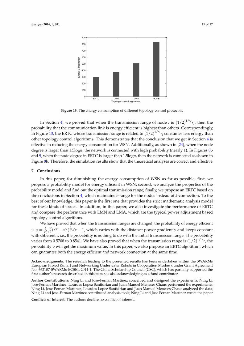
In Section 4, we proved that when the transmission range of node i is 1/γ(1/ 2) ir , then the
probability that the communication link is energy efficient is highest than others. Correspondingly,
in Figure 13, the ERTC whose transmission range is related to 1/γ(1/ 2) ir consumes less energy than
other topology control algorithms. This demonstrates that the conclusion that we get in Section 4 is
effective in reducing the energy consumption for WSN. Additionally, as shown in [24], when the
node degree is larger than 1.5logn , the network is connected with high probability (nearly 1). In
Figures 8b and 9, when the node degree in ERTC is larger than 1.5logn , then the network is
connected as shown in Figure 8b. Therefore, the simulation results show that the theoretical
analyses are correct and effective.
Figure 12. The relationship between node number and node degree in four protocols.
In Figure 12, when the node number smaller than 140, the node degree of ERTC is smaller thanthat of LMA; otherwise, when the node number is larger than 145, the node degree of ERTC is largethan LMA. The reason is that ERTC does not maintain constant node degree which is popular in thetopology control algorithm to guarantee network connection. Maintaining constant neighbors can notreflect the dynamic of WSN, so it can not guarantee that the node works at the optimal transmissionrange which is energy efficient with high probability. As a result, in ERTC, the algorithm maintains ther-range for the node rather than the k-connection. The r-range is the optimal transmission range withhigh probability of energy efficient. In addition, although LMA has stable node degree, the networkperformance of LMA is seriously affected by the node degree thresholds. Moreover, how to set thenode degree threshold has not been discussed strictly in LMA.
Figure 13 displays the energy consumption in different topology control algorithms.From Figure 13, we can conclude that the energy consumption of ERTC is the smallest in thesealgorithms, and ERTC saves approximately 67.4% energy compare with none topology control network.The energy consumption in LMA and LMN are larger than ERTC; moreover, due to LMN can maintainthe node degree in a stable level, so the energy consumption is smaller than LMA. However, the nodedegree in LMN cannot adapt the topology changing.
Energies 2016, 9, 841 15 of 17
Energies 2016, 9, 841 15 of 17
has stable node degree, the network performance of LMA is seriously affected by the node degree
thresholds. Moreover, how to set the node degree threshold has not been discussed strictly in LMA.
50 100 150 2002
4
6
8
10
12
14
16
18
20
22
Node Number
Node D
egre
e
Node degree of orignial network
Node degree of EERTC
Node degree of LMN
Node degree of LMA
Figure 12. The relationship between node number and node degree in four protocols.
Figure 13 displays the energy consumption in different topology control algorithms. From
Figure 13, we can conclude that the energy consumption of ERTC is the smallest in these
algorithms, and ERTC saves approximately 67.4% energy compare with none topology control
network. The energy consumption in LMA and LMN are larger than ERTC; moreover, due to LMN
can maintain the node degree in a stable level, so the energy consumption is smaller than LMA.
However, the node degree in LMN cannot adapt the topology changing.
ERTC LMN LMA NONE0
100
200
300
400
500
600
700
800
900
Topology control algorithms
Energ
y C
onsum
ption
Figure 13. The energy consumption of different topology control protocols.
In Section 4, we proved that when the transmission range of node i is 1/γ(1/ 2) ir , then the
probability that the communication link is energy efficient is highest than others. Correspondingly,
in Figure 13, the ERTC whose transmission range is related to 1/γ(1/ 2) ir consumes less energy than
other topology control algorithms. This demonstrates that the conclusion that we get in Section 4 is
effective in reducing the energy consumption for WSN. Additionally, as shown in [24], when the
node degree is larger than 1.5logn , the network is connected with high probability (nearly 1). In
Figures 8b and 9, when the node degree in ERTC is larger than 1.5logn , then the network is
connected as shown in Figure 8b. Therefore, the simulation results show that the theoretical
analyses are correct and effective.
Figure 13. The energy consumption of different topology control protocols.
In Section 4, we proved that when the transmission range of node i is (1/2)1/γri, then theprobability that the communication link is energy efficient is highest than others. Correspondingly,in Figure 13, the ERTC whose transmission range is related to (1/2)1/γri consumes less energy thanother topology control algorithms. This demonstrates that the conclusion that we get in Section 4 iseffective in reducing the energy consumption for WSN. Additionally, as shown in [24], when the nodedegree is larger than 1.5logn, the network is connected with high probability (nearly 1). In Figures 8band 9, when the node degree in ERTC is larger than 1.5logn, then the network is connected as shown inFigure 8b. Therefore, the simulation results show that the theoretical analyses are correct and effective.
7. Conclusions
In this paper, for diminishing the energy consumption of WSN as far as possible, first, wepropose a probability model for energy efficient in WSN; second, we analyze the properties of theprobability model and find out the optimal transmission range; finally, we propose an ERTC based onthe conclusions in Section 4, which maintains r-range for the nodes instead of k-connection. To thebest of our knowledge, this paper is the first one that provides the strict mathematic analysis modelfor these kinds of issues. In addition, in this paper, we also investigate the performance of ERTCand compare the performance with LMN and LMA, which are the typical power adjustment basedtopology control algorithms.
We have proved that when the transmission ranges are changed, the probability of energy efficient
is ρ = 2r2
∫ r0 (r
γ − xγ)1γ dx− 1, which varies with the distance-power gradient γ and keeps constant
with different r, i.e., the probability is nothing to do with the initial transmission range. The probabilityvaries from 0.5708 to 0.8541. We have also proved that when the transmission range is (1/2)1/γr, theprobability ρ will get the maximum value. In this paper, we also propose an ERTC algotithm, whichcan guarantee both the energy efficient and network connection at the same time.
Acknowledgments: The research leading to the presented results has been undertaken within the SWARMsEuropean Project (Smart and Networking Underwater Robots in Cooperation Meshes), under Grant AgreementNo. 662107-SWARMs-ECSEL-2014-1. The China Scholarship Council (CSC), which has partially supported thefirst author’s research described in this paper, is also acknowledging as a fund contributor.
Author Contributions: Ning Li and Jose-Fernan Martinez conceived and designed the experiments; Ning Li,Jose-Fernan Martinez, Lourdes Lopez Santidrian and Juan Manuel Meneses Chaus performed the experiments;Ning Li, Jose-Fernan Martinez, Lourdes Lopez Santidrian and Juan Manuel Meneses Chaus analyzed the data;Ning Li and Jose-Fernan Martinez contributed analysis tools; Ning Li and Jose Fernan Martinez wrote the paper.
Conflicts of Interest: The authors declare no conflict of interest.

Energies 2016, 9, 841 16 of 17
References
1. Huang, Y.J.; Martinez, J.F.; Diaz, V.H.; Sendra, J. A novel topology control approach to maintain the nodedegree in dynamic wireless sensor networks. Sensors 2014, 14, 4672–4688. [CrossRef] [PubMed]
2. Aziz, A.A.; Sekercioglu, Y.A.; Fitzpatrick, P.; Ivanovich, M. A survey on distributed topology controltechniques for extending the lifetime of battery powered wireless sensor networks. IEEE Commun. Surv. Tutor.2013, 15, 121–144. [CrossRef]
3. Jones, C.E.; Sivalingam, K.M.; Agrawal, P.; Chen, J.C. A survey of energy efficient network protocols forwireless networks. J. Wirel. Netw. 2013, 7, 343–358. [CrossRef]
4. Feeney, L.M.; Nilsson, M. Investigating the energy consumption of a wireless network interface in an ad hocnetworking environment. In Proceedings of the Twentieth Annual Joint Conference of the IEEE Computerand Communications Societies, Anchorage, AK, USA, 22–26 April 2001; pp. 1548–1557.
5. Shen, C.C.; Srisathapornphat, C.; Liu, R.; Huang, Z.; Jaikaeo, C.; Lloyd, E.L. CLTC: A cluster-based topologycontrol for ad hoc networks. IEEE Trans. Mob. Comput. 2004, 3, 18–32. [CrossRef]
6. Miyao, K.; Nakayama, H.; Ansari, N.; Kato, N. LTRT: An efficient and reliable topology control algorithm forad hoc network. IEEE Trans. Wirel. Commun. 2009, 8, 1536–1276. [CrossRef]
7. Kirousis, L.M.; Kranakis, E.; Krizanc, D.; Pelc, A. Power consumption in packet radio networks.Parallel Distrib. Syst. I 1997, 1200, 363–374.
8. Clementi, A.E.F.; Penna, P.; Silvestri, R. On the power assignment problem in radio networks. Mob. Netw. Appl.2004, 9, 125–140. [CrossRef]
9. Bagci, H.; Korpeoglu, I.; Yazici, A. A distributed fault-tolerant topology control algorithm for heterogeneouswireless sensor networks. IEEE Trans. Parallel Distrib. Syst. 2014, 26, 914–923. [CrossRef]
10. Li, M.; Li, Z.J.; Vasilakos, A.V. A survey on topology control in wireless sensor networks: Taxonomy,comparative study, and open issues. Proc. IEEE 2013, 101, 2538–2557. [CrossRef]
11. Huang, Y.J.; Martinez, J.F.; Senda, J.; Lopez, L. Resilient wireless sensor networks using topology control:A review. Sensors 2015, 15, 24735–24770. [CrossRef] [PubMed]
12. Li, N.; Hou, J.C.; Liu, S. Design and analysis of an MST-based topology control algorithm. IEEE Trans.Wirel. Commun. 2015, 4, 1195–1206.
13. Rizvi, S.; Qureshi, H.K.; Khayam, S.A.; Rakocevic, V.; Rajarajan, M. A1: An energy efficient topology controlalgorithm for connected area coverage in wireless sensor networks. J. Netw. Comput. Appl. 2012, 35, 597–605.[CrossRef]
14. Qureshhi, H.K.; Rizvi, S.; Saleem, M.; Khayam, S.A.; Rakocevic, V.; Rajarajan, M. Poly: A reliable and Energyefficient topology control protocol for wireless sensor networks. Comput. Commun. 2011, 34, 1235–1242.[CrossRef]
15. Zhao, J.; Cao, G.H. Robust topology control in multi-hop cognitive radio networks. IEEE Trans. Mob. Comput.2014, 13, 2634–2647. [CrossRef]
16. Ao, X.; Yu, F.R.; Jiang, S.; Guan, Q.; Leung, V.C.M. Distributed cooperative topology control for WANETswith opportunistic interference cancelation. IEEE Trans. Veh. Technol. 2014, 63, 789–801. [CrossRef]
17. Kubisch, M.; Karl, H.; Wolisz, A.; Zhong, L.C. Distributed algorithm for transmission power controlin wireless sensor networks. In Proceedings of the IEEE Wireless Communications and Networking,New Orleans, LA, USA, 16–20 March 2003; pp. 558–563.
18. Chiwewe, T.M.; Hancke, G.P. A distributed topology control technique for low interference and energyefficiency in wireless sensor network. IEEE Trans. Ind. Inform. 2012, 8, 11–19. [CrossRef]
19. Liu, Y.; Ni, L.; Hu, C. A generalized probabilistic topology control for wireless sensor networks. IEEE J. Sel.Areas Commun. 2012, 30, 1780–1788. [CrossRef]
20. Huang, Y.; Martinez, J.F.; Sendra, J.; Lopez, L. The influence of communication range on connectivity forresilient wireless sensor network using a probabilistic approach. Int. J. Distrib. Sens. Netw. 2013, 2013.[CrossRef]
21. Rodoplu, V.; Meng, T.H. Minimum energy mobile wireless networks. IEEE J. Sel. Areas Commun. 2002, 17,1333–1344. [CrossRef]
22. Zhu, Y.; Huang, M.; Chen, S.; Wang, Y. Energy efficient topology control in cooperative ad hoc network.IEEE Trans. Parallel Distrib. Syst. 2012, 23, 1480–1491. [CrossRef]

Energies 2016, 9, 841 17 of 17
23. Rappaport, T.S. Wireless Communication: Principles and Practice; Prentice-Hall: Englewood Cliffs, NJ, USA,1996; pp. 69–122, 139–196.
24. Xue, F.; Kumar, P.R. The number of neighbors needed for connectivity of wireless networks. Wirel. Netw.2004, 10, 169–181. [CrossRef]
25. Parker, R.; Valaee, S. Vehicular node localization using received-signal-strength indicator. IEEE Trans.Veh. Technol. 2007, 56, 3371–3380. [CrossRef]
26. Feng, C.; Au, W.S.A.; Valaee, S.; Tan, Z. Received-signal-strength-based indoor positioning using compressive sensing.IEEE Trans. Mob. Comput. 2012, 11, 1983–1993. [CrossRef]
© 2016 by the authors; licensee MDPI, Basel, Switzerland. This article is an open accessarticle distributed under the terms and conditions of the Creative Commons Attribution(CC-BY) license (http://creativecommons.org/licenses/by/4.0/).