probability in robotics trends in robotics research reactive paradigm (mid-80’s) no models relies...
TRANSCRIPT

Probability in Robotics

Trends in Robotics Research
Reactive Paradigm (mid-80’s)• no models• relies heavily on good sensing
Probabilistic Robotics (since mid-90’s)• seamless integration of models and sensing• inaccurate models, inaccurate sensors
Hybrids (since 90’s)• model-based at higher levels• reactive at lower levels
Classical Robotics (mid-70’s)• exact models• no sensing necessary

Advantages of Probabilistic Paradigm
•Can accommodate inaccurate models•Can accommodate imperfect sensors•Robust in real-world applications•Best known approach to many hard robotics problems•Pays Tribute to Inherent Uncertainty
Know your own ignorance•Scalability•No need for “perfect” world model
Relieves programmers

Limitations of Probability
• Computationally inefficient
– Consider entire probability densities• Approximation
– Representing continuous probability distributions.

Uncertainty Representation

Five Sources of Uncertainty
EnvironmentDynamics
RandomAction Effects
SensorLimitations
InaccurateModels
ApproximateComputation

7
Why Probabilities
Real environments imply uncertainty in accuracy of
robot actions sensor measurements
Robot accuracy and correct models are vital for successful operations
All available data must be used A lot of data is available in the form of
probabilities

8
What Probabilities Sensor parameters Sensor accuracy Robot wheels slipping Motor resolution limited Wheel precision limited Performance alternates based
on temperature, etc.

9
Reasons for Motion Errors
bump
ideal casedifferent wheeldiameters
carpet
and many more …

10
What Probabilities
These inaccuracies can be measured and modelled with random distributions
Single reading of a sensor contains more information given the prior probability distribution of sensor behavior than its actual value
Robot cannot afford throwing away this additional information!

11
What Probabilities
More advanced concepts: Robot position and orientation
(robot pose) Map of the environment Planning and control Action selection Reasoning...

12
Localization, Where am I?
?
• Odometry, Dead Reckoning
• Localization base on external sensors, beacons or landmarks
• Probabilistic Map Based LocalizationObservation
Mapdata base
Prediction of Position
(e.g. odometry)
Perc
epti
on
Matching
Position Update(Estimation?)
raw sensor data or extracted features
predicted position
position
matchedobservations
YES
Encoder
Per
cep
tion

13
Localization Methods
• Mathematic Background, Bayes Filter• Markov Localization:
– Central idea: represent the robot’s belief by a probability distribution over possible positions, and uses Bayes’ rule and convolution to update the belief whenever the robot senses or moves
– Markov Assumption: past and future data are independent if one knows the current state
• Kalman Filtering– Central idea: posing localization problem as a sensor fusion problem– Assumption: gaussian distribution function
• Particle Filtering– Central idea: Sample-based, nonparametric Filter– Monte-Carlo method
• SLAM (simultaneous localization and mapping)• Multi-robot localization

14
Markov Localization• Applying probability theory to robot localization
• Markov localization uses an explicit, discrete representation for the probability of all position in the state space.
• This is usually done by representing the environment by a grid or a topological graph with a finite number of possible states (positions).
• During each update, the probability for each state (element) of the entire space is updated.

15
Markov Localization Example• Assume the robot position is one- dimensional
The robot is placedsomewhere in theenvironment but it is not told its location
The robot queries itssensors and finds out it is next to a door

16
Markov Localization Example
The robot moves one meter forward. To account for inherent noise in robot motion the new belief is smoother
The robot queries itssensors and again it finds itself next to a door

17
Probabilistic Robotics• Falls in between model-based and behavior-
based techniques– There are models, and sensor measurements, but they are
assumed to be incomplete and insufficient for control – Statistics provides the mathematical glue to integrate
models and sensor measurements
• Basic Mathematics– Probabilities– Bayes rule– Bayes filters

Nature of Sensor Data
Odometry Data Range Data


How do we Solve Localization Uncertainty?
• Represent beliefs as a probability density• Markov assumption
Pose distribution at time t conditioned on:pose dist. at time t-1
movement at time t-1
sensor readings at time t
• Discretize the density by
sampling

Probabilistic Action model
• Continuous probability density Bel(st) after moving 40m (left figure) and 80m (right figure). Darker area has higher probablity.
st-1 st-1
at-1
at-1
p(st|at-1,st-1)
At every time step t:UPDATE each sample’s new location based on movement
RESAMPLE the pose distribution based on sensor readings

Globalization
Localization without knowledge of start location

Probabilistic Robotics: Basic Idea
Key idea: Explicit representation of uncertainty using probability theory
• Perception = state estimation• Action = utility optimization

Advantages and Pitfalls
• Can accommodate inaccurate models• Can accommodate imperfect sensors• Robust in real-world applications• Best known approach to many hard robotics problems• Computationally demanding• False assumptions• Approximate

Pr(A) denotes probability that proposition A is true.
Axioms of Probability Theory
1)Pr(0 A
1)Pr( True
)Pr()Pr()Pr()Pr( BABABA
0)Pr( False

A Closer Look at Axiom 3
B
BA A BTrue
)Pr()Pr()Pr()Pr( BABABA

Using the Axioms
)Pr(1)Pr(
0)Pr()Pr(1
)Pr()Pr()Pr()Pr(
)Pr()Pr()Pr()Pr(
AA
AA
FalseAATrue
AAAAAA

Discrete Random Variables
• X denotes a random variable.
• X can take on a finite number of values in {x1, x2, …, xn}.
• P(X=xi), or P(xi), is the probability that the random variable X takes on value xi.
• P( ) is called probability mass function.
• E.g.02.0,08.0,2.0,7.0)( RoomP

Continuous Random Variables
• X takes on values in the continuum.
• p(X=x), or p(x), is a probability density function.
• E.g. b
a
dxxpbax )(]),[Pr(
x
p(x)

Joint and Conditional Probability
• P(X=x and Y=y) = P(x,y)
• If X and Y are independent then
P(x,y) = P(x) P(y)
• P(x | y) is the probability of x given y
P(x | y) = P(x,y) / P(y)
P(x,y) = P(x | y) P(y)
• If X and Y are independent then
P(x | y) = P(x)

Law of Total Probability
y
yxPxP ),()(
y
yPyxPxP )()|()(
x
xP 1)(
Discrete case
1)( dxxp
Continuous case
dyypyxpxp )()|()(
dyyxpxp ),()(

Thomas Bayes (1702-1761)
Clergyman and mathematician who first used probability inductively and established a mathematical basis for probability inference

Bayes Formula
evidence
prior likelihood
)(
)()|()(
)()|()()|(),(
yP
xPxyPyxP
xPxyPyPyxPyxP

Normalization
)()|(
1)(
)()|()(
)()|()(
1
xPxyPyP
xPxyPyP
xPxyPyxP
x
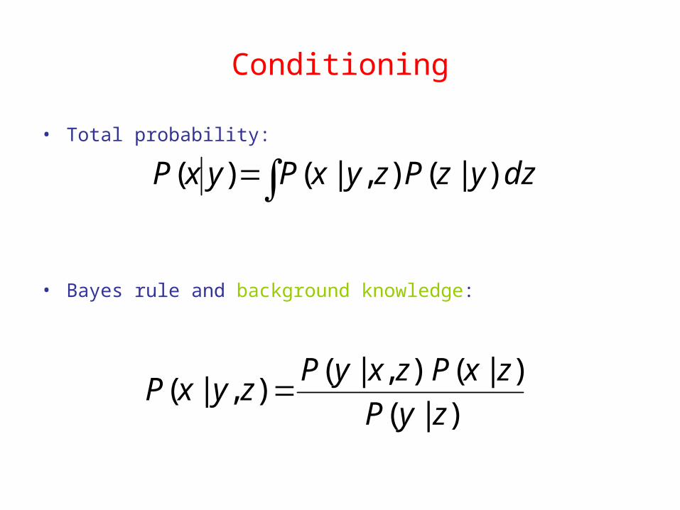
Conditioning
• Total probability:
• Bayes rule and background knowledge:
)|(
)|(),|(),|(
zyP
zxPzxyPzyxP
dzyzPzyxPyxP )|(),|()(

Simple Example of State Estimation
• Suppose a robot obtains measurement z• What is P(open|z)?

Causal vs. Diagnostic Reasoning
• P(open|z) is diagnostic.• P(z|open) is causal.• Often causal knowledge is easier to obtain.• Bayes rule allows us to use causal knowledge:
)()()|(
)|(zP
openPopenzPzopenP
count frequencies!

Example
• P(z|open) = 0.6 P(z|open) = 0.3
• P(open) = P(open) = 0.5
67.03
2
5.03.05.06.0
5.06.0)|(
)()|()()|(
)()|()|(
zopenP
openpopenzPopenpopenzP
openPopenzPzopenP
• z raises the probability that the door is open.

Combining Evidence
• Suppose our robot obtains another observation z2.
• How can we integrate this new information?
• More generally, how can we estimateP(x| z1...zn )?

Recursive Bayesian Updating
),,|(
),,|(),,,|(),,|(
11
11111
nn
nnnn
zzzP
zzxPzzxzPzzxP
Markov assumption: zn is independent of z1,...,zn-1 if we know x.
)()|(
),,|()|(
),,|(
),,|()|(),,|(
...1...1
11
11
111
xPxzP
zzxPxzP
zzzP
zzxPxzPzzxP
ni
in
nn
nn
nnn

Example: Second Measurement
• P(z2|open) = 0.5 P(z2|open) = 0.6
• P(open|z1)=2/3
625.08
5
31
53
32
21
32
21
)|()|()|()|(
)|()|(),|(
1212
1212
zopenPopenzPzopenPopenzP
zopenPopenzPzzopenP
• z2 lowers the probability that the door is open.

Actions
• Often the world is dynamic since
– actions carried out by the robot,– actions carried out by other agents,– or just the time passing by
change the world.
• How can we incorporate such actions?

Typical Actions
• The robot turns its wheels to move• The robot uses its manipulator to grasp an object
• Actions are never carried out with absolute certainty.• In contrast to measurements, actions generally increase the
uncertainty.

Modeling Actions
• To incorporate the outcome of an action u into the current “belief”, we use the conditional pdf
P(x|u,x’)
• This term specifies the pdf that executing u changes the state from x’ to x.

Example: Closing the door

State Transitions
P(x|u,x’) for u = “close door”:
If the door is open, the action “close door” succeeds in 90% of all cases.
open closed0.1 1
0.9
0

Integrating the Outcome of Actions
')'()',|()|( dxxPxuxPuxP
)'()',|()|( xPxuxPuxP
Continuous case:
Discrete case:
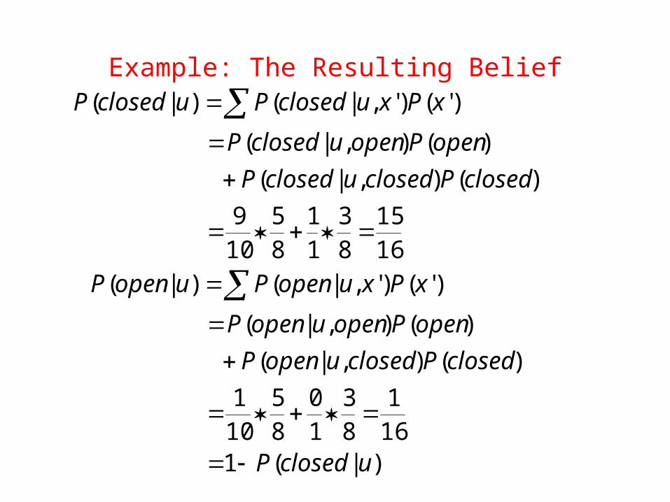
Example: The Resulting Belief
)|(1161
83
10
85
101
)(),|(
)(),|(
)'()',|()|(
1615
83
11
85
109
)(),|(
)(),|(
)'()',|()|(
uclosedP
closedPcloseduopenP
openPopenuopenP
xPxuopenPuopenP
closedPcloseduclosedP
openPopenuclosedP
xPxuclosedPuclosedP
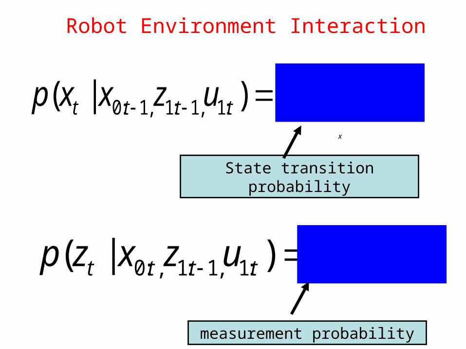
Robot Environment Interaction
x
)|()|( ,1:1,1:1,1:0 ttttttt uxxpuzxxp
State transition probability
)|()|( :1,1:1,:0 tttttt xzpuzxzp
measurement probability

Bayes Filters: Framework
Given: Stream of observations z and action data u:
Sensor model P(z|x). Action model P(x|u,x’). Prior probability of the system state P(x).
Wanted: Estimate of the state X of a dynamical system. The posterior of the state is also called Belief:
),,,|()( 11 tttt zuzuxPxBel
},,,{ 11 ttt zuzud

Markov Assumption
Underlying Assumptions Static world Independent noise Perfect model, no approximation errors
),|(),,|( 1:11:11:1 ttttttt uxxpuzxxp )|(),,|( :11:1:0 tttttt xzpuzxzp

111 )(),|()|( ttttttt dxxBelxuxPxzP
Bayes Filters
),,,,|(),,,,,|( 111111 ttttttt uzzuxPuzzuxzP Bayes
z = observationu = actionx = state
),,,|()( 11 tttt zuzuxPxBel
Markov ),,,,|()|( 111 ttttt uzzuxPxzP
Markov11111 ),,,|(),|()|( ttttttttt dxuzuxPxuxPxzP
11111
1111
),,,,|(
),,,,,|()|(
tttt
tttttt
dxuzzuxP
xuzzuxPxzP
Total prob.
Markov111111 ),,,|(),|()|( tttttttt dxzzuxPxuxPxzP

Bayes Filter Algorithm
• Algorithm Bayes_filter( Bel(x),d ):• 0
• If d is a perceptual data item z then• For all x do• • • For all x do•
• Else if d is an action data item u then• For all x do•
• Return Bel’(x)
)()|()(' xBelxzPxBel )(' xBel
)(')(' 1 xBelxBel
')'()',|()(' dxxBelxuxPxBel
111 )(),|()|()( tttttttt dxxBelxuxPxzPxBel

Bayes Filters are Familiar!
Kalman filters (a recursive Bayesian filter for multivariate normal distributions)
Particle filters (a sequential Monte Carlo (SMC) based technique, which models the PDF using a set of discrete points)
Hidden Markov models (Markov process with unknown parameters)
Dynamic Bayesian networks Partially Observable Markov Decision Processes
(POMDPs)
111 )(),|()|()( tttttttt dxxBelxuxPxzPxBel

Summary Bayes rule allows us to compute probabilities that are
hard to assess otherwise
Under the Markov assumption, recursive Bayesian updating can be used to efficiently combine evidence
Bayes filters are a probabilistic tool for estimating the state of dynamic systems.

How all of this relates to Sensors and navigation?
Micro controller -How to use all these
sensor values
Encoder 1
Gyro 1
Laser
GPS
Gyro 2
Compass
IR
Encoder 2
Ultra sound
Reaction / Decision
Sensor fusion

Basic statistics – Statistical representation – Stochastic variable
Travel time, X = 5hours ±1hour
X can have many different values
[hours]
P
[hours]
P
Discrete variableContinous variable
Continous – The variable can have any value within the bounds
Discrete – The variable can have specific (discrete) values

[hours]
P
Basic statistics – Statistical representation – Stochastic variable
Another way of describing the stochastic variable, i.e. by another form of bounds
In 68%: x11 < X < x12
In 95%: x21 < X < x22
In 99%: x31 < X < x32
In 100%: - < X <
The value to expect is the mean value => Expected value
How much X varies from its expected value => Variance
Probability distribution

Expected value and Variance
0 5 10 15 20 250
1
2
3
4
5
6
7
8Lasting time for 25 battery of the same type
dxxfxXE X )(.
k
X kpkXE )(.
dxxfXExXV XX )(.)( 22
K
XX kpXEkXV )(.)( 22
The standard deviation X is the square root of the variance

Gaussian (Normal) distribution
2
2
2
)(
2.
1)( X
XEx
X
X exp
XXmNX ,~
-10 -5 0 5 10 15 200
0.05
0.1
0.15
0.2
0.25
0.3
0.35
0.4Gaussian distributions with different variances
Stochastic Variable, X
Pro
babi
lity,
p(x
)
N(7,1)N(7,3)N(7,5)N(7,7)
By far the mostly used probability distribution because of its nice statistical and mathematical properties
What does it means if a specification tells that a sensor measures a distance [mm] and has an error that is normally distributed with zero mean and = 100mm?
Normal distribution:
~68.3%
~95%
~99%
etc.
XXXX mm ,
XXXX mm 2,2
XXXX mm 3,3

Estimate of the expected value and the variance from observations
0 1 2 3 4 5 6 7 8 9 100
5
10
15
20
25Histogram of measurements 1 .. 100 of battery lasting time
Lasting time [hours]
No.
of
occu
renc
es [
N]
N
kNX kXm
1
1 )(ˆ
N
kXNX mkX
1
21
12 )ˆ)((̂
-10 -5 0 5 10 15 200
0.05
0.1
0.15
0.2
0.25
0.3
0.35
0.4
Lasting time [hours]
p(x)
Estimated distributionHistogram of observations

Linear combinations (1)
+X1 ~ N(m1, σ1)
X2 ~ N(m2, σ2)
Y ~ N(m1 + m2, sqrt(σ1 +σ2))
bXaEbaXE XVabaXV 2
2121 XEXEXXE 2121 XVXVXXV
Since linear combination of Gaussian variables is another Gaussian variable, Y remains Gaussian if the s.v. are combined linearly!

Linear combinations (2)
DDND ,~ˆ
5
1
151
51
51
51
51
N
iiN DDDDDDY
We measure a distance by a device that have normally distributed errors,
Do we win something of making a lot of measurements and use the average value instead?
What will the expected value of Y be?
What will the variance (and standard deviation) of Y be?
If you are using a sensor that gives a large error, how would you best use it?

Linear combinations (3)
Ground Plane
a(1)
a(i)
X [m]
Y [m]
theta(i)
dii dd ˆ
iiˆ
di is the mean value and d ~ N(0, σd)
αi is the mean value and α ~ N(0, σα)
With d and α un-correlated => V[d, α] = 0 (co-variance is zero)

Linear combinations (4)
N
kN kddddD
121 )(...
N
i
N
i
N
k
N
kd
N
k
N
kd kdkdEEkdEkdEDE
111111
)(0)()(})({ˆ
2
11111
0)(})({ˆd
N
kd
N
k
N
kd
N
k
N
kd NVVkdVkdVDV
D = {The total distance} is calculated as before as this is only the sum of all d’s
The expected value and the variance become:

Linear combinations (5)
= {The heading angle} is calculated as before as this is only the sum of all ’s, i.e. as the sum of all changes in heading
The expected value and the variance become:
1
000 )()1(...)1()0(
N
k
kN
1
0
1
0
)()0()}()({))0()0((ˆN
k
N
k
kkkEE
1
0
1
0
)()0()}()({))0()0((ˆN
k
N
k
kVVkkVV
What if we want to predict X and Y from our measured d’s and ’s?

Non-linear combinations (1)
)cos( 1111 NNNNN dXX
X(N) is the previous value of X plus the latest movement (in the X direction)
The estimate of X(N) becomes:
)cos()()()ˆˆcos(ˆˆˆ11111111 11 NNdNXNNNNNN NN
dXdXX
)cos(11
iN N
This equation is non-linear as it contains the term:
and for X(N) to become Gaussian distributed, this equation must be replaced with a linear approximation around . To do this we can use the Taylor expansion of the first order. By this approximation we also assume that the error is rather small!With perfectly known N-1 and N-1 the equation would have been linear!
11 NN

Non-linear combinations (2)
)sin()()cos()()(
)cos()()(ˆ
111111
1111
11
11
NNNNdNXN
NNdNXNN
NN
NN
dX
dXX
Use a first order Taylor expansion and linearize X(N) around .11 NN
This equation is linear as all error terms are multiplied by constants and we can calculate the expected value and the variance as we did before.
)cos()cos(
)sin()()cos()()(ˆ
11111111
111111 11
NNNNNNNN
NNNNdNXNN
dXdEXE
dXEXENN

Non-linear combinations (3)
The variance becomes (calculated exactly as before):
221
22221
2
11
11
11
11
11
)sin()cos()sin(
)sin()()cos()(
)sin()()cos()()(ˆ
NN
NN
NN
NdNX
dNXN
dNXNN
dd
dVVXV
dXVXV
Two really important things should be noticed, first the linearization only affects the calculation of the variance and second (which is even more important) is that the above equation is the partial derivatives of:
)ˆˆcos(ˆˆˆ1111 NNNNN dXX with respect to our uncertain
parameters squared multiplied with their variance!
Non-linear combinations (4)
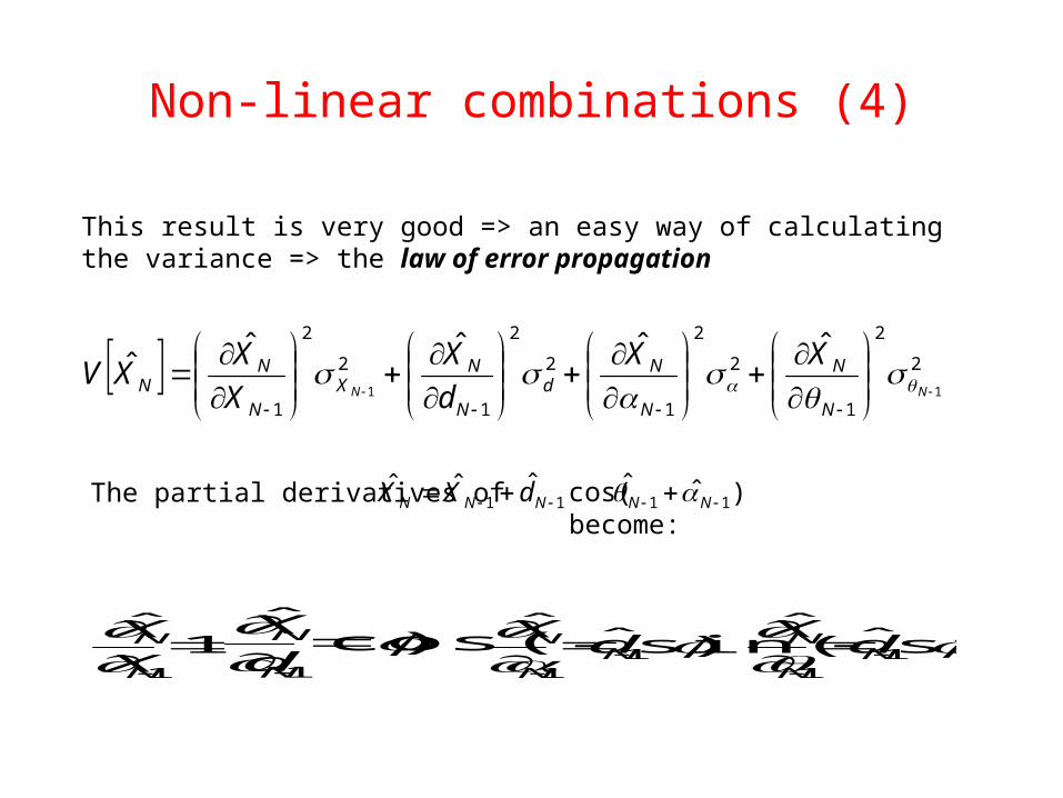
This result is very good => an easy way of calculating the variance => the law of error propagation
2
2
1
2
2
1
2
2
1
2
2
111
ˆˆˆˆˆ
NN
N
N
N
Nd
N
NX
N
NN
XX
d
X
X
XXV
1ˆ
1
N
N
X
X )cos(ˆ
1
N
N
d
X)sin(ˆ
ˆ1
1
NN
N dX
)sin(ˆˆ
11
NN
N dX
The partial derivatives of become:)ˆˆcos(ˆˆˆ1111 NNNNN dXX

Non-linear combinations (5)
-1000 -500 0 500 1000 1500 2000 2500 30000
0.1
0.2
0.3
0.4
0.5
0.6
0.7Estimated X and its variance
X [km]
P(X
)
The plot shows the variance of X for the time step 1, …, 20 and as can be noticed the variance (or standard deviation) is constantly increasing.
d = 1/10
= 5/360
5.02
0X

The Error Propagation Law

The Error Propagation Law

The Error Propagation Law

Multidimensional Gaussian distributions MGD (1)
)()( 121
21
)2(
1)( XX
TX mxmx
XNX exp
23
22
21
2,31,3
3,21,2
3,12,1
x
x
x
X
xxCxxC
xxCxxC
xxCxxC
The Gaussian distribution can easily be extended for several dimensions by: replacing the variance () by a co-variance matrix () and the scalars (x and mX) by column vectors.
The CVM describes (consists of):
1) the variances of the individual dimensions => diagonal elements
2) the co-variances between the different dimensions => off-diagonal elements
! Symmetric
! Positive definite

2
2
2
)(
2
1)(
x
exP
A 1-d Gaussian distribution is given by:
)()(2
1 1
||)2(
1)(
xx
n
T
exP
An n-d Gaussian distribution is given by:

MGD (2)
-250 -200 -150 -100 -50 0 50 100 150 200 250-250
-200
-150
-100
-50
0
50
100
150
200
250
X
Y
Un-correlated S.V.
STD of X is 10 times bigger than STD of YSTD of Y is 5 times bigger than STD of X
-250 -200 -150 -100 -50 0 50 100 150 200 250-250
-200
-150
-100
-50
0
50
100
150
200
250
X
Y
Correlated S.V.
STD of X is 10 times bigger than STD of YSTD of Y is 5 times bigger than STD of X
25000
0100)(green
25754287
42877525)(red
19001039
1039700)(green
25000
0100)(red
Eigenvalues => standard deviations
Eigenvectors => rotation of the ellipses

MGD (3)
))((, YX mYmXEYXC
j k
YXYX kjpmkmjYXC ),())((, ,
dxdyyxfmymxYXC YXYX ),())((, ,
The co-variance between two stochastic variables is calculated as:
Which for a discrete variable becomes:
And for a continuous variable becomes:
K
XX kpXEkXV )(.)( 22

MGD (4) - Non-linear combinations
Ground Plane
a(1)
a(i)
X [m]
Y [m]
theta(i)
)()(
))()(sin()()(
))()(cos()()(
))(),((
)1(
)1(
)1(
)1(
kk
kkkdky
kkkdkx
kUkZf
k
ky
kx
kZ
The state variables (x, y, ) at time k+1 become:

MGD (5) - Non-linear combinations
TUU
TXX fkUffkkfkk )1()|()|1(
)()(
))()(sin()()(
))()(cos()()(
))(),((
)1(
)1(
)1(
)1(
kk
kkkdky
kkkdkx
kUkZf
k
ky
kx
kZ
We know that to calculate the variance (or co-variance) at time step k+1 we must linearize Z(k+1) by e.g. a Taylor expansion - but we also know that this is done by the law of error propagation, which for matrices becomes:
100
))()(cos()(10
))()(sin()(01
kkkd
kkkd
f X
10
))()(cos()())()(sin(
))()(sin()())()(cos(
kkkdkk
kkkdkk
fU
With fX and fU are the Jacobian matrices (w.r.t. our uncertain variables) of the state transition matrix.

MGD (6) - Non-linear combinations
0 200 400 600 800 1000 1200 1400 1600
-200
0
200
400
600
800
1000
Airplane taking off, relative displacement in each time step = (100km, 2deg)
X [km]
Y [
km
]
The uncertainty ellipses for X and Y (for time step 1 .. 20) is shown in the figure.
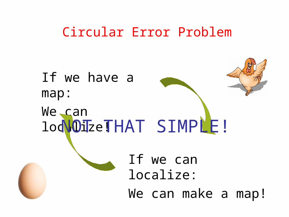
Circular Error Problem
If we have a map:We can localize!
If we can localize:We can make a map!
NOT THAT SIMPLE!
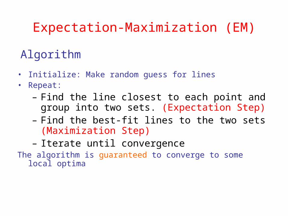
Expectation-Maximization (EM)
• Initialize: Make random guess for lines• Repeat:
– Find the line closest to each point and group into two sets. (Expectation Step)
– Find the best-fit lines to the two sets (Maximization Step)
– Iterate until convergenceThe algorithm is guaranteed to converge to some local optima
Algorithm

Example:

Example:

Example:
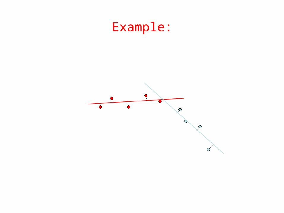
Example:

Example:
Converged!

Probabilistic Mapping
• E-Step: Use current best map and data to find belief probabilities• M-step: Compute the most likely map based on the probabilities
computed in the E-step.• Alternate steps to get better map and localization estimates
Convergence is guaranteed as before.
Maximum Likelihood Estimation

The E-Step
• P(st|d,m) = P(st |o1, a1… ot,m) . P(st |at…oT,m)
t Bel(st)Markov Localization
t
Analogous to but computed
backward in time

The M-Step
• Updates occupancy grid
• P(mxy=l | d) =
# of times l was observed at <x,y>
# of times something was obs. at <x,y>
T
t Lltttttxy
T
ttttttxy
dssolmP
dssolmP
1 '
1
),|'(
),|(

Probabilistic Mapping
• Addresses the Simultaneous Mapping and Localization problem (SLAM)
• Robust• Hacks for easing computational and processing burden
– Caching– Selective computation– Selective memorization


Markov Assumption
Future is Independent of Past Given Current State
“Assume Static World”

Probabilistic Model
)|()( 0 ttt dspsBel
),,,,,,( 11100...0 toaoaoad tt
Action Data Observation Data

Derivation : Markov Localization
1111 )(),|()|()( tttttttt dssBelasspsopsBel
),,,,|()( 011 ooaospsBel ttttt
),,,|(),,,,|( 011011 ooaspooasop ttttttt Bayes
),,,|()|( 011 ooaspsop ttttt Markov
110111 )|(),|()|( tttttttt dsdspasspsop
Markov
1021111 ),,|(),|()|( ttttttttt dsoaospasspsop
1011011 ),,|(),,,|()|( tttttttt dsoaspoasspsop Total Probability

Mobile Robot Localization•Proprioceptive Sensors: (Encoders, IMU) - Odometry, Dead reckoning•Exteroceptive Sensors: (Laser, Camera) - Global, Local Correlation
Scan-Matching
Scan 1 Scan 2
Iterate
Displacement Estimate
Initial Guess
Point Correspondence
Scan-Matching
•Correlate range measurements to estimate displacement•Can improve (or even replace) odometry – Roumeliotis TAI-14•Previous Work - Vision community and Lu & Milios [97]

1 mx500
Weighted Approach
Explicit models of uncertainty & noise sources for each scan point:
• Sensor noise & errors• Range noise • Angular uncertainty• Bias
• Point correspondence uncertainty
Correspondence Errors
Improvement vs. unweighted method:• More accurate displacement estimate• More realistic covariance estimate• Increased robustness to initial conditions• Improved convergence
CombinedUncertanties

Weighted Formulation
Error between kth scan point pair
Measured range data from poses i and j
sensor noise
Goal: Estimate displacement (pij ,ij )
bias true range
= rotation of ij
Correspondence ErrorNoise Error Bias Error

Lik
l
1) Sensor Noise
Covariance of Error Estimate
Covariance of error between kth scan point pair =
2) Sensor Bias
neglect for now
Pose i
CorrespondenceSensor Noise Bias

3) Correspondence Error = cijk
Estimate bounds of cijk from the geometry
of the boundary and robot poses
•Assume uniform distribution
Max error
where

Finding incidence angles ik and j
k
Hough Transform
-Fits lines to range data
-Local incidence angle estimated from line tangent and scan angle
-Common technique in vision community (Duda & Hart [72])
-Can be extended to fit simple curves
Scan PointsFit Lines
ik

Likelihood of obtaining errors {ijk} given displacement
Maximum Likelihood Estimation
•Position displacement estimate obtained in closed form
•Orientation estimate found using 1-D numerical optimization, or series expansion approximation methods
Non-linear Optimization Problem

Experimental Results
• Increased robustness to inaccurate initial displacement guesses
•
Fewer iterations for convergence
Weighted vs. Unweighted matching of two poses
512 trials with different initial displacements within : +/- 15 degrees of actual angular displacement+/- 150 mm of actual spatial displacement
Initial DisplacementsUnweighted EstimatesWeighted Estimates

Unweighted Weighted

Displacement estimate errors at end of path
• Odometry = 950mm• Unweighted = 490mm• Weighted = 120mm
Eight-step, 22 meter path
More accurate covariance estimate- Improved knowledge of measurement uncertainty- Better fusion with other sensors

Uncertainty From Sensor Noiseand Correspondence Error
1 m
x500