Probability (cont.)

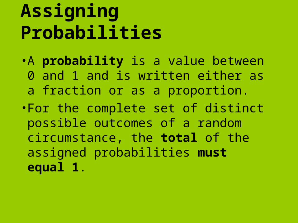
Assigning Probabilities

• A probability is a value between 0 and 1 and is written either as a fraction or as a proportion.

• For the complete set of distinct possible outcomes of a random circumstance, the total of the assigned probabilities must equal 1.

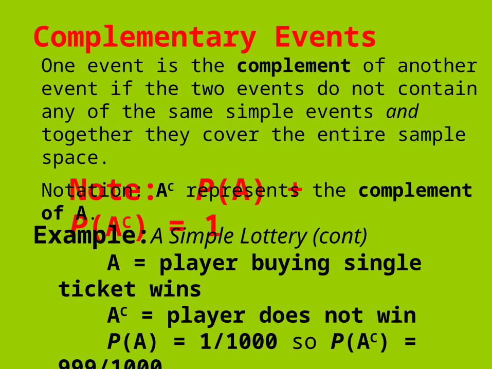
Complementary Events

Note: P(A) + P(AC) = 1

One event is the complement of another event if the two events do not contain any of the same simple events and together they cover the entire sample space.

Notation: AC represents the complement of A.

Example:A Simple Lottery (cont)A = player buying single ticket winsAC = player does not winP(A) = 1/1000 so P(AC) = 999/1000

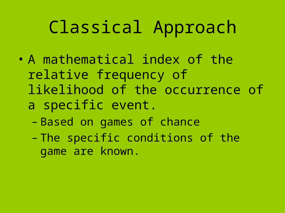
Classical Approach

• A mathematical index of the relative frequency of likelihood of the occurrence of a specific event.– Based on games of chance– The specific conditions of the game are

known.

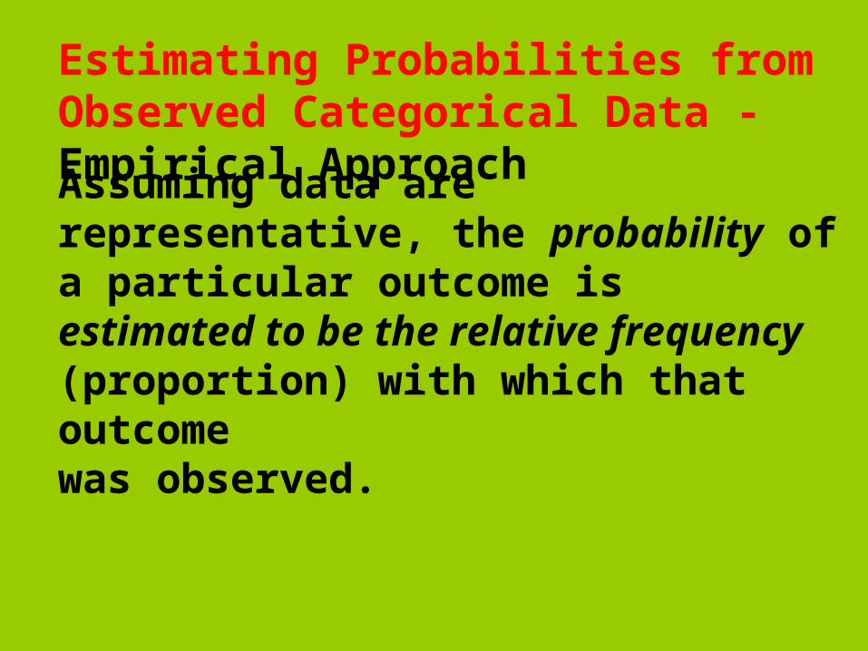
Estimating Probabilities from Observed Categorical Data - Empirical Approach

Assuming data are representative, the probability of a particular outcome is estimated to be the relative frequency (proportion) with which that outcome was observed.

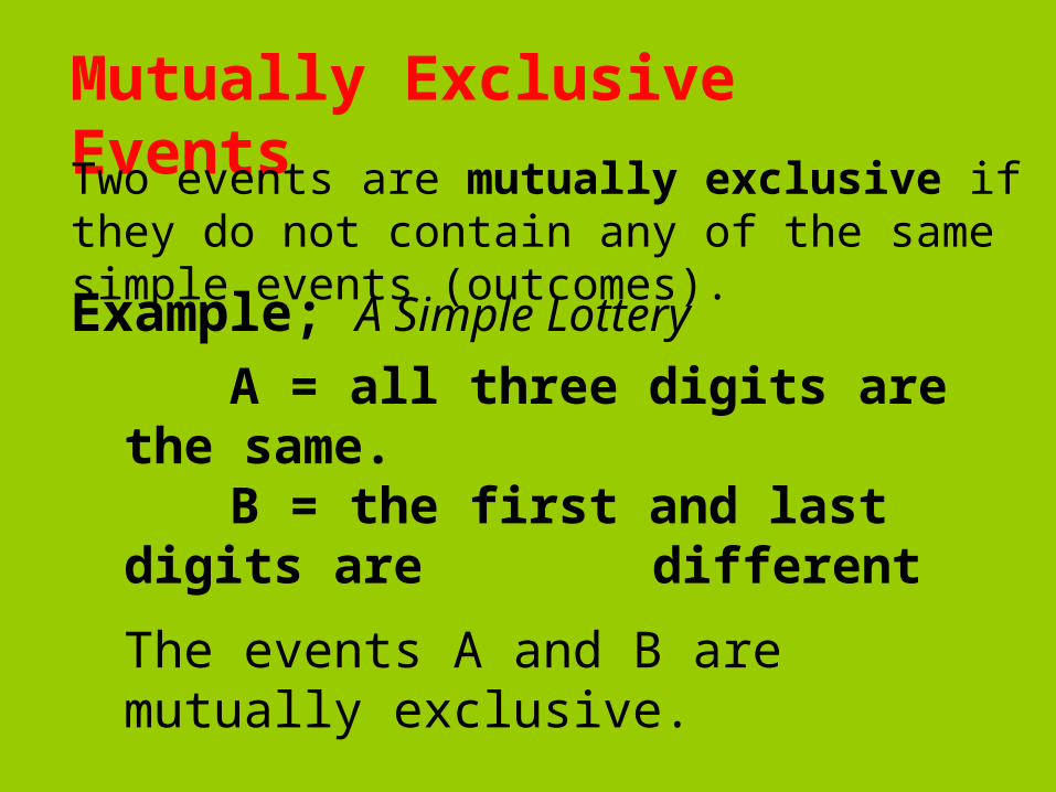
Mutually Exclusive Events

Two events are mutually exclusive if they do not contain any of the same simple events (outcomes).

Example; A Simple Lottery

A = all three digits are the same.B = the first and last digits are different

The events A and B are mutually exclusive.

Independent and Dependent Events• Two events are independent of each other

if knowing that one will occur (or has occurred) does not change the probability that the other occurs.

• Two events are dependent if knowing that one will occur (or has occurred) changes the probability that the other occurs.

Example Independent Events •Customers put business card in restaurant glass bowl. •Drawing held once a week for free lunch. •You and Vanessa put a card in two consecutive wks.

Event A = You win in week 1.Event B = Vanessa wins in week 2

• Events A and B refer to to different random circumstances and are independent.

Event A = Alicia is selected to answer Question 1.Event B = Alicia is selected to answer Question 2.

• P(A) = 1/50.• If event A occurs, her name is no longer in the bag; P(B) = 0.• If event A does not occur, there are 49 names in the

bag (including Alicia’s name), so P(B) = 1/49.

Events A and B refer to different random circumstances, but are A and B independent events?

Knowing whether A occurred changes P(B). Thus, the events A and B are not independent.

Example: Dependent Events

Probability Calculations

• Some Useful Formulas to Keep in Mind (Or in Hand)– U = Union (or)

– ∩ = Intersection (and)

• General FormulasAdding (“or)

P(A U B) = P(A) + P(B) – P(A ∩ B)

Non-mutually Exclusive of Overlapping Outcomes.

P(A U B) = P(A) + P(B)

Mutually Exclusive Outcomes

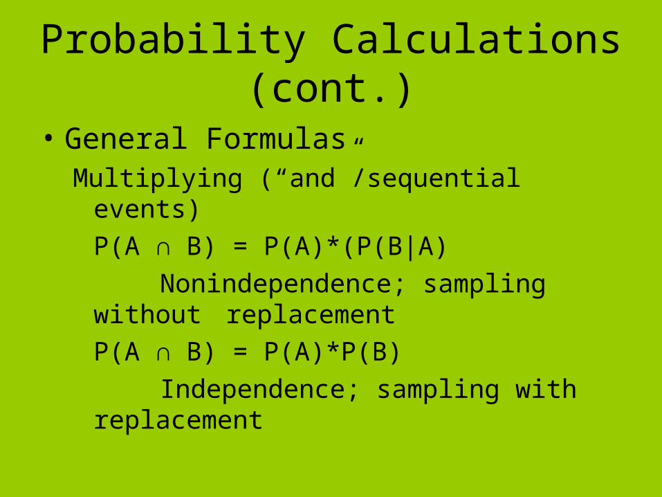
Probability Calculations (cont.)

• General FormulasMultiplying (“and”/sequential events)

P(A ∩ B) = P(A)*(P(B|A)

Nonindependence; sampling without replacement

P(A ∩ B) = P(A)*P(B)

Independence; sampling with replacement

Joint and Marginal Probabilities

• These probabilities refer to the proportion of an event as a fraction of the total.

P(30 to 64) = 62,689/103,870 = .60P(30 to 64 ∩ married) = 43,308/103,870 = .42

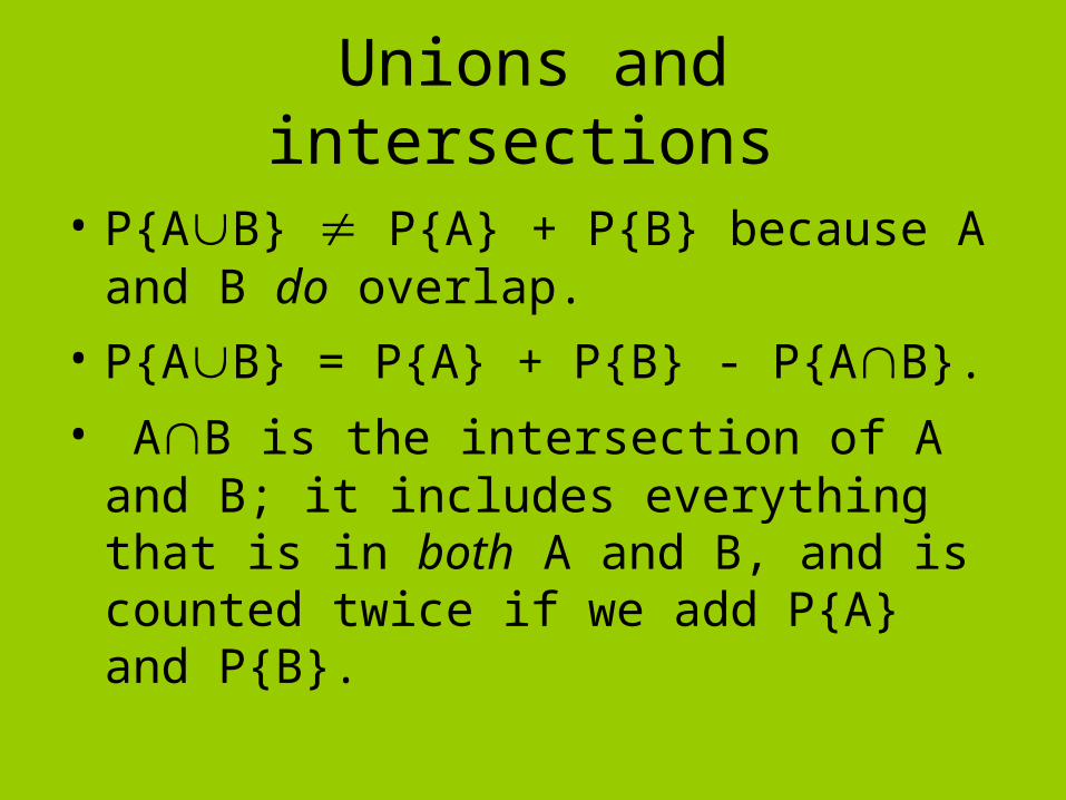
Unions and intersections

• P{AB} P{A} + P{B} because A and B do overlap.

• P{AB} = P{A} + P{B} - P{AB}.

• AB is the intersection of A and B; it includes everything that is in both A and B, and is counted twice if we add P{A} and P{B}.

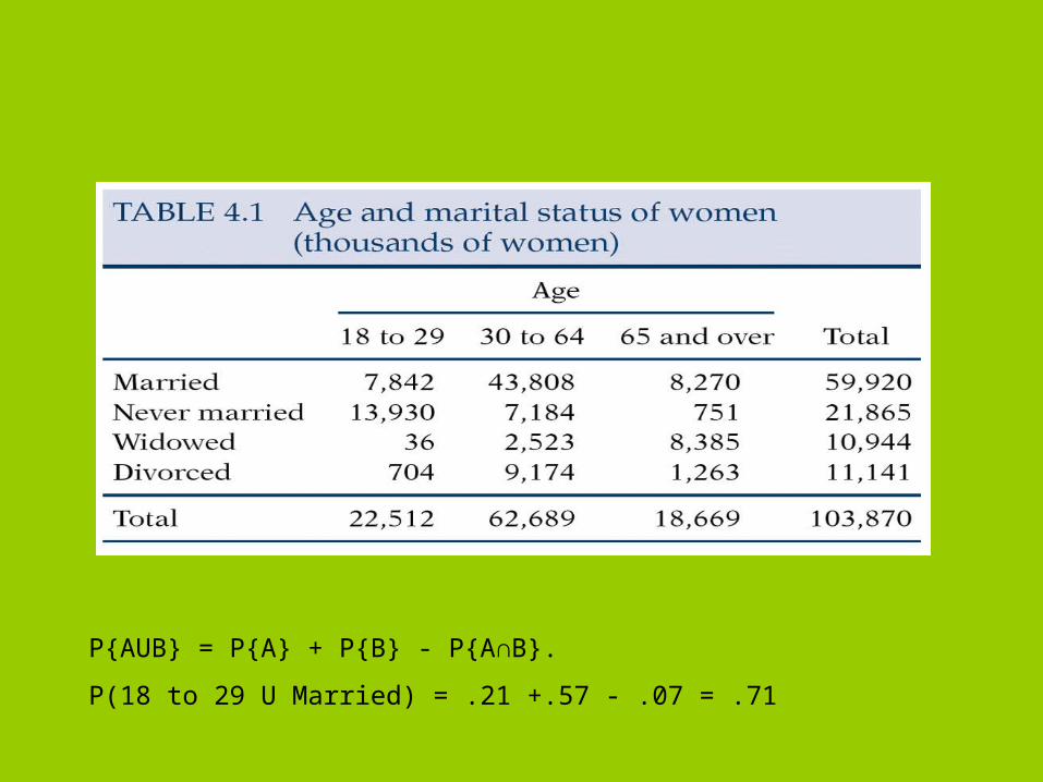
P{AUB} = P{A} + P{B} - P{A∩B}.

P(18 to 29 U Married) = .21 +.57 - .07 = .71

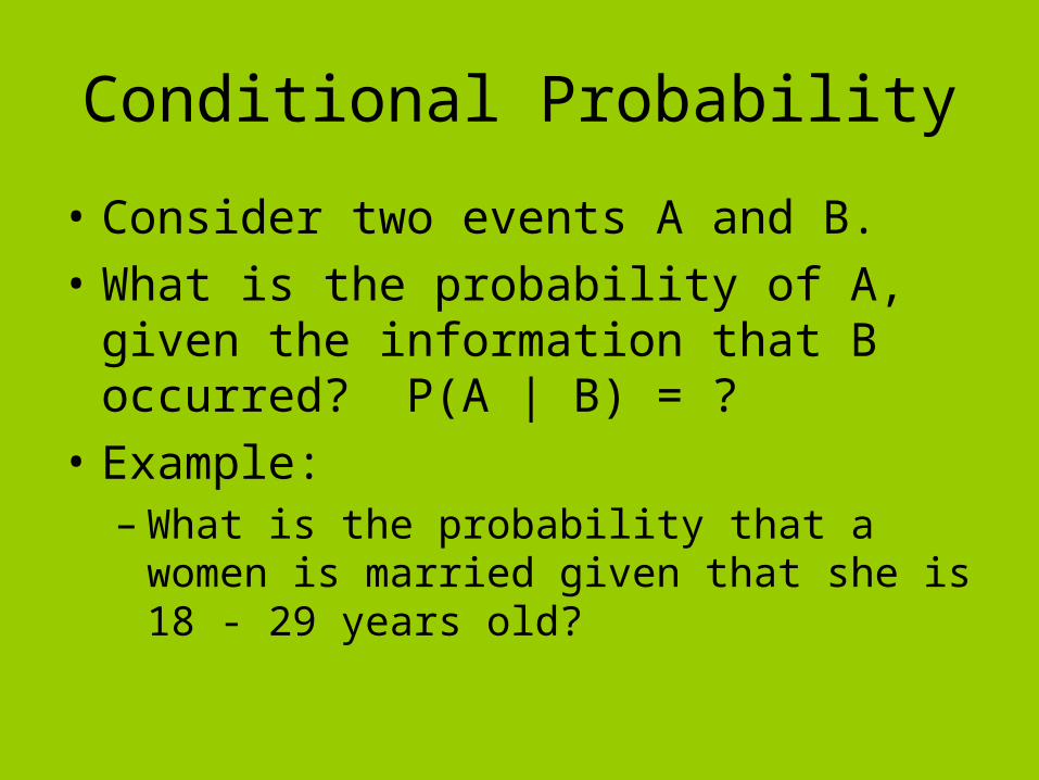
Conditional Probability

• Consider two events A and B.

• What is the probability of A, given the information that B occurred? P(A | B) = ?

• Example:– What is the probability that a women is

married given that she is 18 - 29 years old?

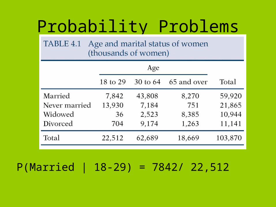
Probability Problems

P(Married | 18-29) = 7842/ 22,512

Conditional probability and independence

• If we know that one event has occurred it may change our view of the probability of another event. Let – A = {rain today}, B = {rain tomorrow}, C = {rain in 90 days time}

• It is likely that knowledge that A has occurred will change your view of the probability that B will occur, but not of the probability that C will occur.

• We write P(B|A) P(B), P(C|A) = P(C). P(B|A) denotes the conditional probability of B, given A.

• We say that A and C are independent, but A and B are not.

• Note that for independent events P(AC) = P(A)P(C).

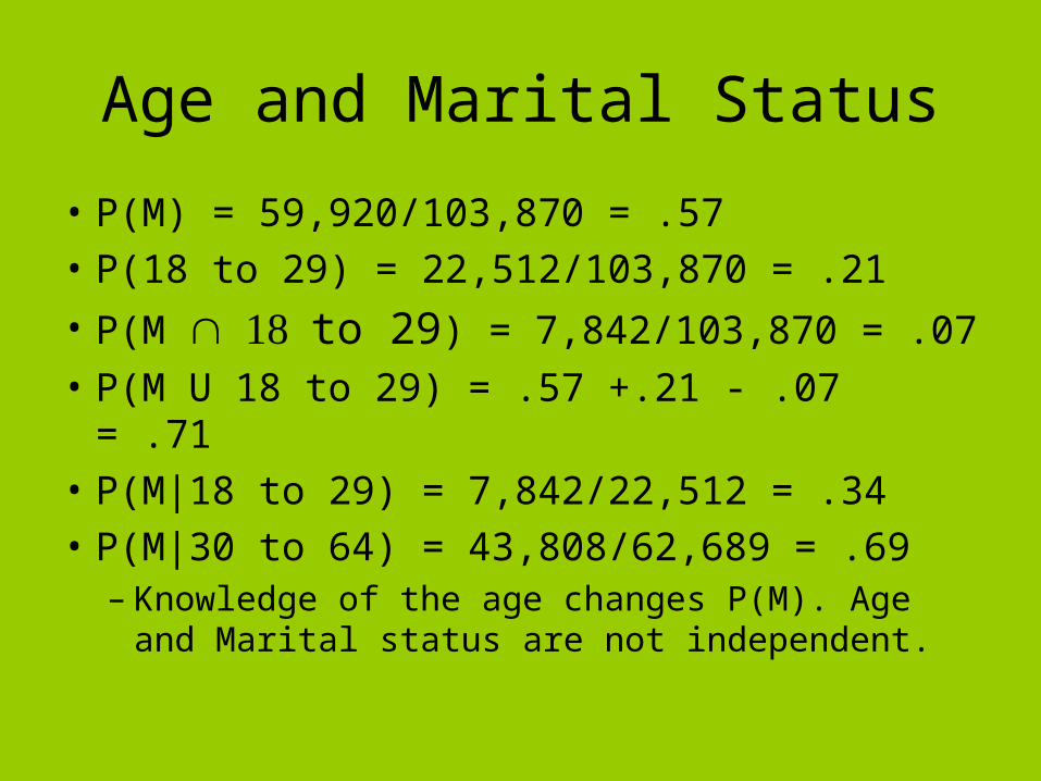
Age and Marital Status

• P(M) = 59,920/103,870 = .57

• P(18 to 29) = 22,512/103,870 = .21

• P(M to 29) = 7,842/103,870 = .07

• P(M U 18 to 29) = .57 +.21 - .07 = .71

• P(M|18 to 29) = 7,842/22,512 = .34

• P(M|30 to 64) = 43,808/62,689 = .69– Knowledge of the age changes P(M). Age and

Marital status are not independent.

Group Practice

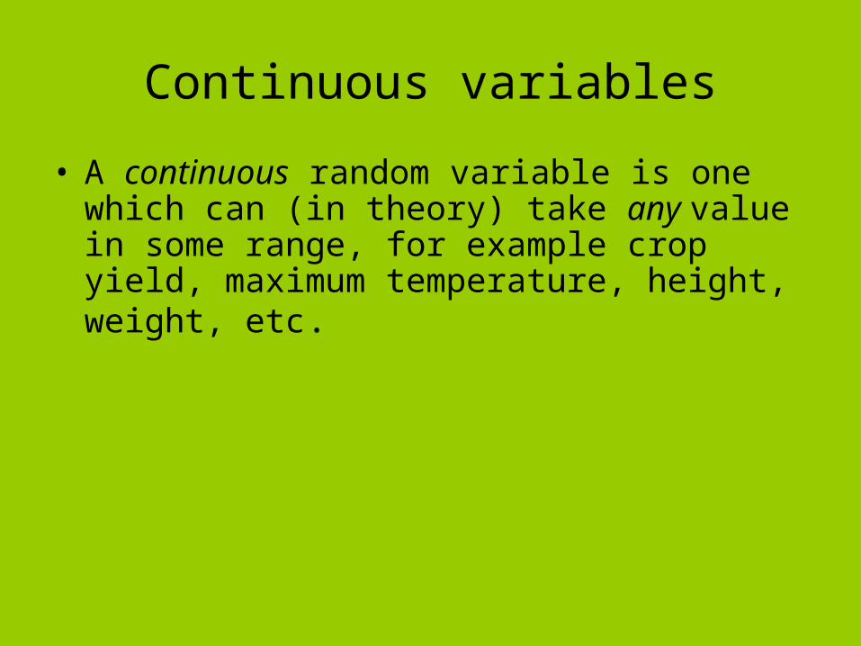
Continuous variables

• A continuous random variable is one which can (in theory) take any value in some range, for example crop yield, maximum temperature, height, weight, etc.

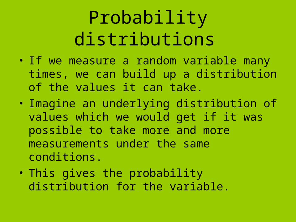
Probability distributions

• If we measure a random variable many times, we can build up a distribution of the values it can take.

• Imagine an underlying distribution of values which we would get if it was possible to take more and more measurements under the same conditions.

• This gives the probability distribution for the variable.

Continuous probability distributions

• Because continuous random variables can take all values in a range, it is not possible to assign probabilities to individual values.

• Instead we have a continuous curve, called a probability density function, which allows us to calculate the probability a value within any interval.

• This probability is calculated as the area under the curve between the values of interest. The total area under the curve must equal 1.

Normal (Gaussian) distributions

• Normal (also known as Gaussian) distributions are by far the most commonly used family of continuous distributions.

• They are ‘bell-shaped’ –and are indexed by two parameters:– The mean – the distribution is symmetric about this

value – The standard deviation – this determines the spread

of the distribution. Roughly 2/3 of the distribution lies within 1 standard deviation of the mean, and 95% within 2 standard deviations.

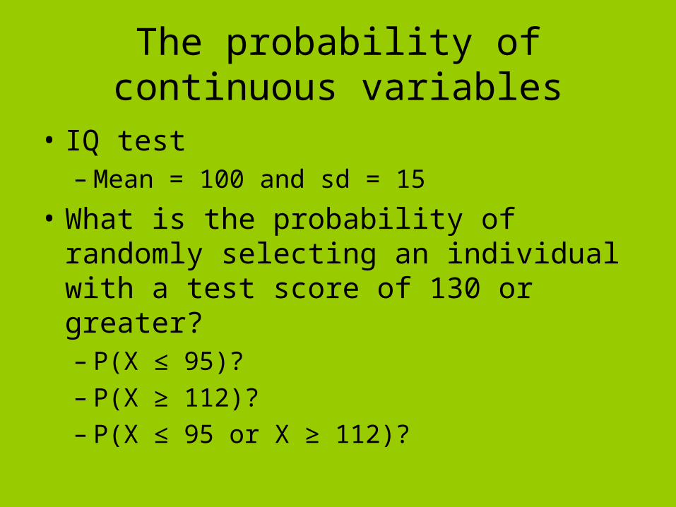
The probability of continuous variables

• IQ test– Mean = 100 and sd = 15

• What is the probability of randomly selecting an individual with a test score of 130 or greater?– P(X ≤ 95)?– P(X ≥ 112)?– P(X ≤ 95 or X ≥ 112)?

The probability of continuous variables (cont.)

• What is the probability of randomly selecting three people with a test score greater than 112?– Remember the multiplication rule for

independent events.

Introduction to Statistical Inference

Chapter 11

Populations vs. Samples

• Population– The complete set of individuals

• Characteristics are called parameters

• Sample– A subset of the population

• Characteristics are called statistics.

– In most cases we cannot study all the members of a population

Inferential Statistics

• Statistical Inference– A series of procedures in which the data

obtained from samples are used to make statements about some broader set of circumstances.

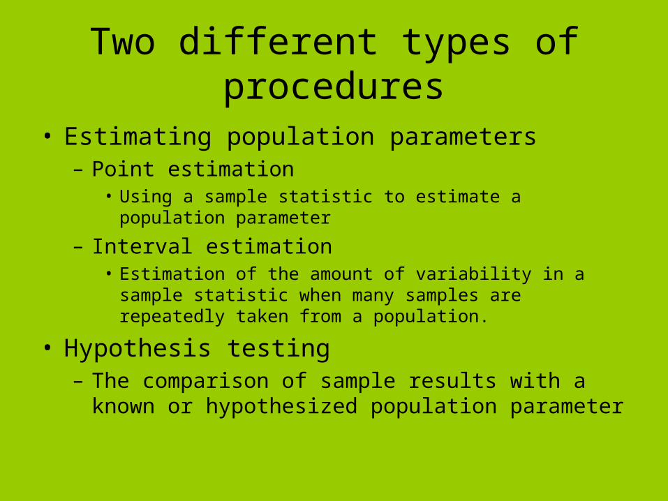
Two different types of procedures

• Estimating population parameters– Point estimation

• Using a sample statistic to estimate a population parameter

– Interval estimation• Estimation of the amount of variability in a sample statistic

when many samples are repeatedly taken from a population.

• Hypothesis testing– The comparison of sample results with a known or

hypothesized population parameter

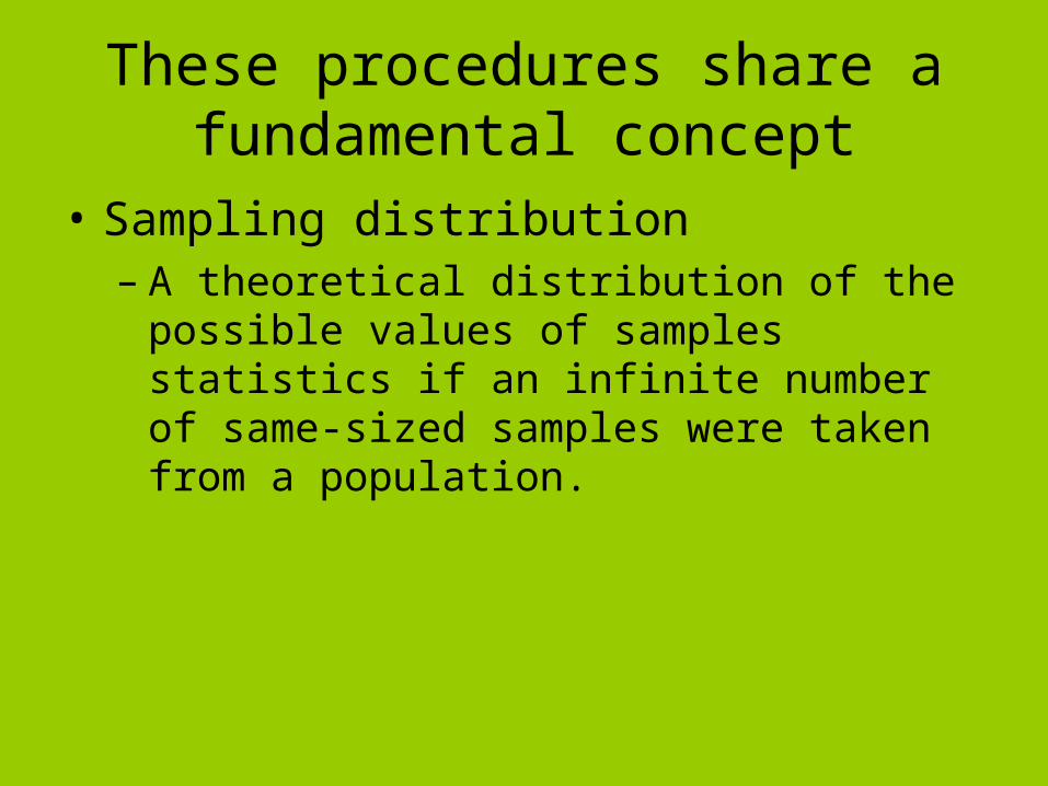
These procedures share a fundamental concept

• Sampling distribution– A theoretical distribution of the possible

values of samples statistics if an infinite number of same-sized samples were taken from a population.

Example of the sampling distribution of a discrete variable

Binomial sampling distribution of an unbiased coin tossed 10 times

0

0.05

0.1

0.150.2

0.25

0.3

0 1 2 3 4 5 6 7 8 9 10

Number of heads in 10 tosses

p(x

)

Continuous Distributions

• Interval or ratio level data– Weight, height, achievement, etc.

• JellyBlubbers!!!

Histogram of the Jellyblubber population

Repeated sampling of the Jellyblubber population (n = 3)

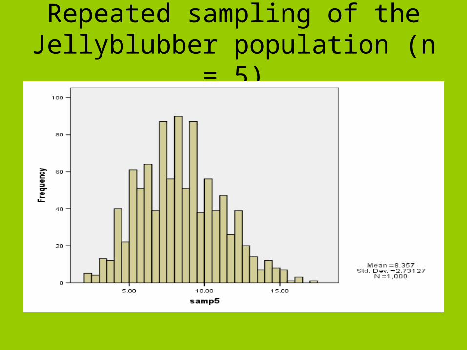
Repeated sampling of the Jellyblubber population (n = 5)

Repeated sampling of the Jellyblubber population (n = 10)

Repeated sampling of the Jellyblubber population (n = 40)

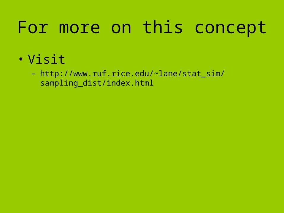
For more on this concept

• Visit– http://www.ruf.rice.edu/~lane/stat_sim/sampling_dist/index.html

Central Limit Theorem

• Proposition 1:– The mean of the sampling

distribution will equal the mean of the population.

• Proposition 2:– The sampling distribution of

means will be approximately normal regardless of the shape of the population.

• Proposition 3:– The standard deviation

(standard error) equals the standard deviation of the population divided by the square root of the sample size. (see 11.5 in text)

x

Nx

Application of the sampling distribution

• Sampling error– The difference between the sample mean and the population

mean.• Assumed to be due to random error.

• From the jellyblubber experience we know that a sampling distribution of means will be randomly distributed with

x Nx

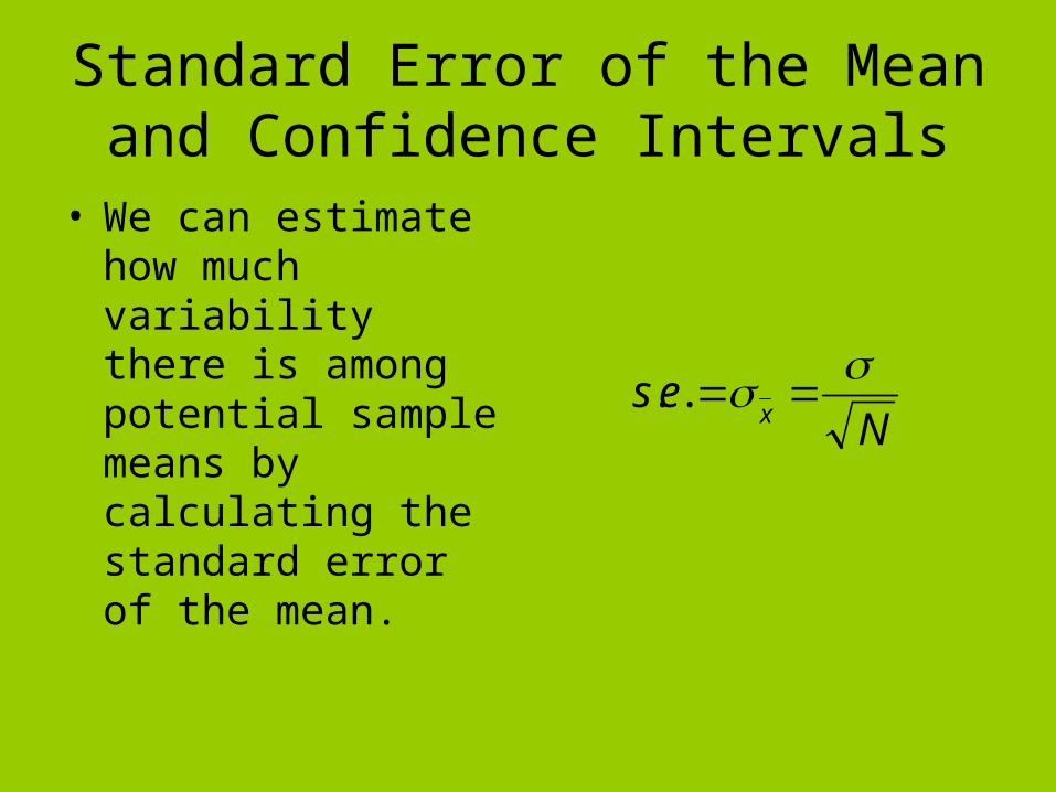
Standard Error of the Mean and Confidence Intervals

• We can estimate how much variability there is among potential sample means by calculating the standard error of the mean.

Nes

x

..

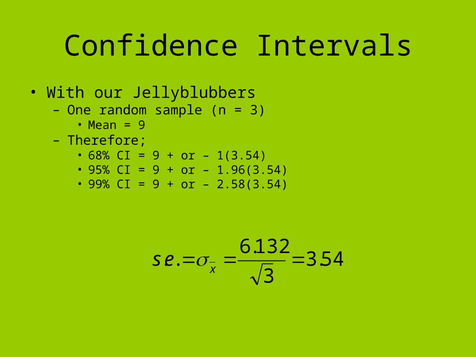
Confidence Intervals

• With our Jellyblubbers– One random sample (n = 3)

• Mean = 9– Therefore;

• 68% CI = 9 + or – 1(3.54)• 95% CI = 9 + or – 1.96(3.54)• 99% CI = 9 + or – 2.58(3.54)

54.33

132.6..

xes

Confidence Intervals

• With our Jellyblubbers– One random sample (n = 30)

• Mean = 8.90– Therefore;

• 68% CI = 8.90 + or – 1(1.11)• 95% CI = 8.90 + or – 1.96(1.11)• 99% CI = 8.90 + or – 2.58(1.11)

11.130

132.6..

xes

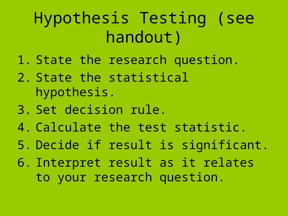
Hypothesis Testing (see handout)

1. State the research question.

2. State the statistical hypothesis.

3. Set decision rule.

4. Calculate the test statistic.

5. Decide if result is significant.

6. Interpret result as it relates to your research question.