probability and statistics (first half): math10013maotj/notes/prob10013.pdf · a first course in...
TRANSCRIPT

Probability and Statistics (first half): MATH10013
Professor Oliver [email protected]
Twitter: @BristOliver
School of Mathematics, University of Bristol
Teaching Block 1, 2019
Oliver Johnson ([email protected]) Probability and Statistics: @BristOliver TB 1 c©UoB 2019 1 / 272
Why study probability?
Probability began from the study of gambling and games of chance.
It took hundreds of years to be placed on a completely rigorousfooting.
Now probability is used to analyse physical systems, model financialmarkets, study algorithms etc.
The world is full of randomness and uncertainty: we need tounderstand it!
Oliver Johnson ([email protected]) Probability and Statistics: @BristOliver TB 1 c©UoB 2019 2 / 272

Course outline
22+2 lectures, 6 exercise classes (odd weeks), 6 mandatory HW sets(even weeks).
2 online quizzes (Weeks 5, 9) count 5% towards final module mark.
IT IS YOUR RESPONSIBILITY TO ATTEND LECTURESAND TO ENSURE YOU HAVE A FULL SET OF NOTES ANDSOLUTIONS
Course webpage for notes, problem sheets, links etc:https://people.maths.bris.ac.uk/∼maotj/prob.htmlDrop-in sessions: Tuesday 1-2. Just turn up to Room G83 FryBuilding in these times. (Other times, I may be out or busy - but justemail [email protected] to fix an appointment).
This material is copyright of the University unless explicitly statedotherwise. It is provided exclusively for educational purposes at theUniversity and is to be downloaded or copied for your private studyonly.
Oliver Johnson ([email protected]) Probability and Statistics: @BristOliver TB 1 c©UoB 2019 3 / 272
Contents
1 Introduction
2 Section 1: Elementary probability
3 Section 2: Counting arguments
4 Section 3: Conditional probability
5 Section 4: Discrete random variables
6 Section 5: Expectation and variance
7 Section 6: Joint distributions
8 Section 7: Properties of mean and variance
9 Section 8: Continuous random variables I
10 Section 9: Continuous random variables II
11 Section 10: Conditional expectation
1 Section 11: Moment generating functions
Oliver Johnson ([email protected]) Probability and Statistics: @BristOliver TB 1 c©UoB 2019 4 / 272
Textbook
The recommended textbook for the unit is:A First Course in Probability by S. Ross.
Copies are available in the Queens Building library.
Oliver Johnson ([email protected]) Probability and Statistics: @BristOliver TB 1 c©UoB 2019 5 / 272
Section 1: Elementary probability
Objectives: by the end of this section you should be able to
Define events and sample spaces, describe them in simpleexamplesDescribe combinations of events using set-theoretic notationList the axioms of probabilityState and use simple results such as inclusion–exclusion and deMorgan’s Law
Oliver Johnson ([email protected]) Probability and Statistics: @BristOliver TB 1 c©UoB 2019 6 / 272

Section 1.1: Random events
[This material is also covered in Sections 2.1 and 2.2 of the course book]
Definition 1.1.
Random experiment or trial. Examples:I spin of a roulette wheelI throw of a diceI London stock market running for a day
A sample point or elementary outcome ω is the result of a trial:I the number on the roulette wheelI the number on the diceI the observed position of the stock market at the end of the day
The sample space Ω is the set of all possible elementary outcomes ω.
Oliver Johnson ([email protected]) Probability and Statistics: @BristOliver TB 1 c©UoB 2019 7 / 272
Red and green dice
Example 1.2.
Consider the experiment of throwing a red die and a green die.
Represent an elementary outcome as a pair, such as
ω = (6, 3)
where the first number is the score on the red die and the secondnumber is the score on the green die.
Then the sample space
Ω = (1, 1), (1, 2), . . . , (6, 6)
has 36 sample points.
Note we use set notation: this will be key for us.
Oliver Johnson ([email protected]) Probability and Statistics: @BristOliver TB 1 c©UoB 2019 8 / 272

Events
Definition 1.3.
An event is a set of outcomes specified by some condition.
Note that events are subsets of the sample space, denoted A ⊆ Ω.
We say that event A occurs if the elementary outcome of the trial liesin the set A, denoted ω ∈ A.
Example 1.4.
In the red and green dice example, Example 1.2, let A be the event thatthe sum of the scores is 5:
A = (1, 4), (2, 3), (3, 2), (4, 1).
Oliver Johnson ([email protected]) Probability and Statistics: @BristOliver TB 1 c©UoB 2019 9 / 272
Two special cases
Remark 1.5.
There are two special events:
A = ∅, the empty set. This event never occurs, since we can neverhave ω ∈ ∅.A = Ω, the whole sample space. This event always occurs, since wealways have ω ∈ Ω.
Oliver Johnson ([email protected]) Probability and Statistics: @BristOliver TB 1 c©UoB 2019 10 / 272

Combining events.
Given two events A and B, we can combine them together, usingstandard set notation.
Informal description Formal description
A occurs or B occurs (or both) A ∪ BA and B both occur A ∩ BA does not occur Ac
A occurs implies B occurs A ⊆ BA and B cannot both occur together A ∩ B = ∅(disjoint or mutually exclusive)
You may find it useful to represent combinations of events using Venndiagrams.
Oliver Johnson ([email protected]) Probability and Statistics: @BristOliver TB 1 c©UoB 2019 11 / 272
Example: draw a lottery ball.
Example 1.6.
The trial is to draw one ball in the lottery.
An elementary outcome is ω = k , where k is the observed numberdrawn. Ω = 1, 2, . . . , 59.Example events
Event Informal description Formal description
A an odd number is drawn A = 1, 3, 5, . . . , 59B an even number is drawn B = 2, 4, 6, . . . , 58C number is divisible by 3 C = 3, 6, 9, . . . , 57
We then haveEvent Informal description Formal description
A or C odd or divisible by 3 A ∪ C = 1, 3, 5, 6, 7, 9, . . . , 57, 59B and C div by 2 and 3 B ∩ C = 6, 12, . . . , 54
Oliver Johnson ([email protected]) Probability and Statistics: @BristOliver TB 1 c©UoB 2019 12 / 272
Section 1.2: Axioms of probability
[This material is also covered in Section 2.3 of the course book.]
We have an intuitive idea that some events are more likely thanothers.
Tossing a head is more likely than winning the lottery.
The probability P captures this.
Oliver Johnson ([email protected]) Probability and Statistics: @BristOliver TB 1 c©UoB 2019 13 / 272
Axioms of probability
Definition 1.7.
Suppose we have a sample space Ω.
Let P be a map from events A ⊆ Ω to the real numbers R.
For each event A (each subset of Ω) there is a number P(A).
Then P is a probability measure if it satisfies:
Axiom 1 0 ≤ P(A) ≤ 1 for every event A.Axiom 2 P(Ω) = 1.Axiom 3 Let A1,A2, . . . be an infinite collection of disjoint events
(so Ai ∩ Aj = ∅ for all i 6= j). Then
P
( ∞⋃i=1
Ai
)= P(A1) + P(A2) + · · · =
∞∑i=1
P(Ai ).
Oliver Johnson ([email protected]) Probability and Statistics: @BristOliver TB 1 c©UoB 2019 14 / 272
Deductions from the axioms
These three axioms form the basis of all probability theory.
We will develop the consequences of these axioms as a rigorousmathematical theory, using only logic.
We show that it matches our intuition for how we expect probabilityto behave.
Example 1.8.
From these 3 axioms it is simple to prove the following:
Property 1 P(∅) = 0
Property 2 For a finite collection of disjoint events A1, . . . ,An,
P
(n⋃
i=1
Ai
)= P(A1) + P(A2) + · · ·+ P(An) =
n∑i=1
P(Ai ).
Property 2 follows from Axiom 3 by taking Ai = ∅ for i ≥ n + 1.
Oliver Johnson ([email protected]) Probability and Statistics: @BristOliver TB 1 c©UoB 2019 15 / 272
Motivating the axioms
Suppose we have a sample space Ω, and an event A ⊆ Ω.
For example, if we roll a 6-sided dice then Ω = 1, 2, . . . , 6, andconsider the event A = 6 (the roll gives a 6).
Suppose the trial is repeated infinitely many times, and let an be thenumber of times A occurs in the first n trials.
We might expect ann to converge to a limit as n→∞, which
provisionally we might call Prob(A).
Assuming it does converge, it is clear thatI 0 ≤ Prob(A) ≤ 1I Prob(Ω) = 1I Prob(∅) = 0
Oliver Johnson ([email protected]) Probability and Statistics: @BristOliver TB 1 c©UoB 2019 16 / 272

Motivating the axioms (cont.)
Furthermore, if A and B are disjoint events, and C = A ∪ B, for thefirst n trials let
I an be the number of times A occursI bn be the number of times B occursI cn be the number of times C occurs
Then cn = an + bn since A and B are disjoint.
Thereforeann
+bnn
=cnn.
Taking the limit as n→∞ we see that
Prob(A) + Prob(B) = Prob(C ) = Prob(A ∪ B).
Oliver Johnson ([email protected]) Probability and Statistics: @BristOliver TB 1 c©UoB 2019 17 / 272
Motivating the axioms (cont.)
Remark 1.9.
However, how can we know if these limits exist?
It seems intuitively reasonable, but we can’t be sure.
The modern theory of probability works the other way round: wesimply assume that for each event A there exists a number P(A),where P is assumed to obey the axioms of Definition 1.7.
Oliver Johnson ([email protected]) Probability and Statistics: @BristOliver TB 1 c©UoB 2019 18 / 272

Section 1.3: Some simple applications of the axioms
[This material is also covered in Section 2.4 of the course book.]
Lemma 1.10.
For any event A, the complement satisfies P(Ac) = 1− P(A)
Proof.
By definition, A and Ac are disjoint events: that is A ∩ Ac = ∅.Further, Ω = A ∪ Ac , so P(Ω) = P(A) + P(Ac) by Property 2.
But P(Ω) = 1, by Axiom 2. So 1 = P(A) + P(Ac).
Oliver Johnson ([email protected]) Probability and Statistics: @BristOliver TB 1 c©UoB 2019 19 / 272
Some simple applications of the axioms (cont.)
Lemma 1.11.
Let A ⊆ B. Then P(A) ≤ P(B).
Proof.
We can write B = A ∪ (B ∩ Ac), and A ∩ (B ∩ Ac) = ∅.That is, A and B ∩ Ac are disjoint events.
Hence by Property 2 we have P(B) = P(A) + P(B ∩ Ac).
But by Axiom 1 we have P(B ∩ Ac) ≥ 0, so P(B) ≥ P(A).
Oliver Johnson ([email protected]) Probability and Statistics: @BristOliver TB 1 c©UoB 2019 20 / 272

Inclusion–exclusion principle n = 2
Lemma 1.12.
Let A and B be any two events. Then
P(A ∪ B) = P(A) + P(B)− P(A ∩ B).
Proof.
A ∪ B = A ∪ (B ∩ Ac) is a disjoint union, so
P(A ∪ B) = P(A) + P(B ∩ Ac) (Property 2). (1.1)
B = (B ∩ A) ∪ (B ∩ Ac) is a disjoint union, so
P(B) = P(B ∩ A) + P(B ∩ Ac) (Property 2). (1.2)
Subtracting (1.2) from (1.1) we haveP(A ∪ B)− P(B) = P(A)− P(A ∩ B).
Oliver Johnson ([email protected]) Probability and Statistics: @BristOliver TB 1 c©UoB 2019 21 / 272
General inclusion–exclusion principle
Consider a collection of events A1, . . . ,An.
Given a subset S ⊆ 1, . . . , n, write⋂
j∈S Aj for an intersectionindexed by that subset.
For example: if S = 1, 3 then⋂
j∈S Aj = A1⋂A3.
Theorem 1.13.
For n events A1, . . . ,An, we can write
P
(n⋃
i=1
Ai
)=
n∑k=1
(−1)k+1∑
S :|S |=k
P
⋂j∈S
Aj
,
where the sum over S covers all subsets of 1, 2, . . . , n of size k.
Proof.
Not proved here (check how for n = 2 it reduces to Lemma 1.12?)
Oliver Johnson ([email protected]) Probability and Statistics: @BristOliver TB 1 c©UoB 2019 22 / 272

Inclusion–exclusion example
Example 1.14.
In the sports club,
36 members play tennis, 22 play tennis and squash,28 play squash, 12 play tennis and badminton,18 play badminton, 9 play squash and badminton,
4 play tennis, squash and badminton.
How many play at least one of these games?
Introduce probability by picking a random member out of those Nenrolled to the club. Then
T : = that person plays tennis,S : = that person plays squash,B : = that person plays badminton.
Oliver Johnson ([email protected]) Probability and Statistics: @BristOliver TB 1 c©UoB 2019 23 / 272
Example 1.14.
Applying Theorem 1.13 with n = 3 we obtain
P(T ∪ S ∪ B) = P(T ) + P(S) + P(B)
−P(T ∩ S)− P(T ∩ B)− P(S ∩ B)
+P(T ∩ S ∩ B)
=36
N+
28
N+
18
N− 22
N− 12
N− 9
N+
4
N=
43
N.
Our answer is therefore 43 members.
Note that in some sense, we don’t need probability here – there is aversion of inclusion–exclusion just for set sizes.
Oliver Johnson ([email protected]) Probability and Statistics: @BristOliver TB 1 c©UoB 2019 24 / 272
Boole’s inequality – ‘union bound’
Proposition 1.15 (Boole’s inequality).
For any events A1, A2, . . . , An,
P
(n⋃
i=1
Ai
)≤
n∑i=1
P(Ai ).
Oliver Johnson ([email protected]) Probability and Statistics: @BristOliver TB 1 c©UoB 2019 25 / 272
Boole’s inequality proof
Proof.
Proof by induction. When n = 2, by Lemma 1.12:
P (A1 ∪ A2) = P(A1) + P(A2)− P(A1 ∩ A2) ≤ P(A1) + P(A2).
Now suppose true for n. Then
P
(n+1⋃i=1
Ai
)= P
((n⋃
i=1
Ai
)∪ An+1
)≤ P
(n⋃
i=1
Ai
)+ P(An+1)
≤n∑
i=1
P(Ai ) + P(An+1) =n+1∑i=1
P(Ai ).
Oliver Johnson ([email protected]) Probability and Statistics: @BristOliver TB 1 c©UoB 2019 26 / 272

Key idea: de Morgan’s Law
Theorem 1.16.
For any events A and B:
(A ∪ B)c = Ac ∩ Bc (1.3)
(A ∩ B)c = Ac ∪ Bc (1.4)
Proof.
Draw a Venn diagram.Note that (swapping A and Ac , and swapping B and Bc), (1.3) and (1.4)are equivalent.
Remark 1.17.
(1.3)‘Neither A nor B happens’ same as ’A doesn’t happen and Bdoesn’t happen’.
(1.4) ‘A and B don’t both happen’ same as ‘either A doesn’t happen,or B doesn’t’
Oliver Johnson ([email protected]) Probability and Statistics: @BristOliver TB 1 c©UoB 2019 27 / 272
Key idea: de Morgan’s Law
Theorem 1.18.
For any events A and B:
1− P (A ∪ B) = P (Ac ∩ Bc) (1.5)
1− P (A ∩ B) = P (Ac ∪ Bc) (1.6)
Proof.
Since the events on either side of (1.3) are the same, they must havethe same probability.
Further, we know from Lemma 1.10 that P(E c) = 1− P(E ) for anyevent E .
A similar argument applies to (1.4).
By a similar argument, can extend (1.5) and (1.6) to collections of nevents.
Oliver Johnson ([email protected]) Probability and Statistics: @BristOliver TB 1 c©UoB 2019 28 / 272

Example
Example 1.19.
Return to Example 1.2: suppose we roll a red die and a green die.
What is the probability that we roll a 6 on at least one of them?
Write A = roll a 6 on red die, B = roll a 6 on green die.Event ‘roll a 6 on at least one’ is A ∪ B.
Hence by (1.5),
P(A ∪ B) = 1− P (Ac ∩ Bc) = 1− 5
6· 5
6=
11
36,
since P (Ac ∩ Bc) = P(Ac)P(Bc) = (1− P(A))(1− P(B))
Caution: This final step only works because two rolls are‘independent’ (see later for much more on this!!)
Oliver Johnson ([email protected]) Probability and Statistics: @BristOliver TB 1 c©UoB 2019 29 / 272
Example: tossing a coin to obtain a head.
Example 1.20.
A fair coin is tossed repeatedly until the first head is obtained.
We will find the probability that an odd number of tosses is required.
For this random experiment a sample point is just a positive integercorresponding to the total number of throws required to get the firsthead. Thus
Ω = 1, 2, 3, 4, . . .
Let Ak denote the event that exactly k tosses are required, i.e.Ak = k.Assume that P(Ak) = 1
2k(will see how to justify this properly later).
Oliver Johnson ([email protected]) Probability and Statistics: @BristOliver TB 1 c©UoB 2019 30 / 272

Example: tossing a coin to obtain a head (cont).
Example 1.20.
Let B denote the event that the number of tosses required is odd.Thus
B = A1 ∪ A3 ∪ A5 ∪ . . . .
Since the Ak ’s are disjoint
P(B) = P(A1) + P(A3) + P(A5) + . . .
=1
2+
1
23+
1
25+ . . .
=1
2
[1 +
1
4+
1
42+ . . .
]=
1
2
[1
(1− 14 )
]=
2
3.
Oliver Johnson ([email protected]) Probability and Statistics: @BristOliver TB 1 c©UoB 2019 31 / 272
Section 2: Counting arguments
Objectives: by the end of this section you should be able to
Understand how to calculate probabilities when there are equallylikely outcomesDescribe outcomes in the language of combinations andpermutationsCount these outcomes using factorial notation
Oliver Johnson ([email protected]) Probability and Statistics: @BristOliver TB 1 c©UoB 2019 32 / 272
Section 2.1: Equally likely sample points
[This material is also covered in Section 2.5 of the course book]
A common case that arises is where each of the sample points has thesame probability.
This can often be justified by physical symmetry and the use ofProperty 2.
For example, think of rolling a dice.
There are 6 disjoint sample outcomes, and symmetry says they haveequal probability.
Hence Property 2 tells us that P(i) = 1/6 for i = 1, . . . , 6.
In such cases calculating probability reduces to a counting problem.
Oliver Johnson ([email protected]) Probability and Statistics: @BristOliver TB 1 c©UoB 2019 33 / 272
More formally
Assume thatI Ω, the sample space, is finiteI all sample points are equally likely
Then by Axiom 2 and Property 2, considering the disjoint unionP(⋃
ω∈Ωω)
we can see that
P(ω) =1
Number of points in Ω=
1
|Ω|.
Also, if A ⊆ Ω, then considering P(⋃
ω∈Aω)
P(A) =Number of points in A
Number of points in Ω=|A||Ω|
.
Hence, we need to learn to count!
Oliver Johnson ([email protected]) Probability and Statistics: @BristOliver TB 1 c©UoB 2019 34 / 272
Example: red and green dice.
Example 2.1.
A red die and a green die are rolled.
A sample point is ω = (r , g) where r is the score on the red dice andg is the score on the green dice.
The whole sample space
Ω = (1, 1), (1, 2), . . . , (6, 6)
with 36 sample points.
By arguments like the above, assume that P(ω) = 136 for each ω
(i.e. equally likely outcomes).
Oliver Johnson ([email protected]) Probability and Statistics: @BristOliver TB 1 c©UoB 2019 35 / 272
Example: red and green dice. (cont)
Example 2.1.
Let A5 be the event that the sum of the scores is 5:
A5 = (1, 4), (2, 3), (3, 2), (4, 1) = (1, 4)∪(2, 3)∪(3, 2)∪(4, 1)
a disjoint union.
Then
P(A5) = P((1, 4)) + P((2, 3)) + P((3, 2)) + P((4, 1))
=1
36+
1
36+
1
36+
1
36=
1
9.
Exercise: For each i , let Ai be the event that the sum of the scores isi . Show that
P(A4) =1
12, P(A3) =
1
18, P(A2) =
1
36.
Oliver Johnson ([email protected]) Probability and Statistics: @BristOliver TB 1 c©UoB 2019 36 / 272

Example: red and green dice. (cont)
Example 2.1.
Let B be the event that the sum of the scores is less than or equal to5. Then
B = A2 ∪ A3 ∪ A4 ∪ A5
a disjoint union. So
P(B) = P(A2)+P(A3)+P(A4)+P(A5) =1
36+
2
36+
3
36+
4
36=
10
36=
5
18
Let C be the event that the sum of the scores is greater than 5. Wecould calculate P(A6), . . . , P(A12). But it’s easier to spot thatC = Bc , so
P(C ) = 1− P(B) = 1− 5
18=
13
18.
Oliver Johnson ([email protected]) Probability and Statistics: @BristOliver TB 1 c©UoB 2019 37 / 272
Section 2.2: Permutations and combinations
[This material is also covered by Sections 1.1 - 1.4 of the course book.]
Definition 2.2.
A permutation is a selection of r objects from n ≥ r objects when theordering matters.
Oliver Johnson ([email protected]) Probability and Statistics: @BristOliver TB 1 c©UoB 2019 38 / 272

Permutations example
Example 2.3.
Eight swimmers in a race, how many different ways of allocating the threemedals are there?
Gold medal winner can be chosen in 8 ways.
For each gold medal winner, the silver medal can go to one of theother 7 swimmers, so there are 8× 7 different options for gold andsilver.
For each choice of first and second place, the bronze medal can go toone of the other 6 swimmers, so there are 8× 7× 6 different ways themedals can be handed out.
Oliver Johnson ([email protected]) Probability and Statistics: @BristOliver TB 1 c©UoB 2019 39 / 272
General theory
Lemma 2.4.
In general there are nPr = n(n − 1)(n − 2) · · · (n − r + 1) differentways.
Note that we can write nPr = n!(n−r)! .
General convention: 0! = 1
Remark 2.5.
Check the special cases:
r = n: nPn = n!(n−n)! = n!
1 = n!, so there are n! ways of ordering nobjects.
r = 1: nP1 = n!(n−1)! = n, so there are n ways of choosing 1 of n
objects.
Oliver Johnson ([email protected]) Probability and Statistics: @BristOliver TB 1 c©UoB 2019 40 / 272

BRISTOL example1
Example 2.6.
How many four letter ’words’ can be formed from distinct letters ofthe word BRISTOL? (i.e. no letter used more than once)There are 7 distinct letters in BRISTOL. Hence the first letter can bechosen in 7 ways, the second in 6 ways, etc.There are then 7× 6× 5× 4 = 840 = 7!
(7−4)! words.
1This kind of analysis was first performed by al-Farahidi in Iraq in the 8th CenturyOliver Johnson ([email protected]) Probability and Statistics: @BristOliver TB 1 c©UoB 2019 41 / 272
BANANA example
Example 2.7.
In how many ways can the letters of the word BANANA berearranged to produce distinct 6-letter “words”?There are 6! orderings of the letters of the word BANANA.But can order the 3 As in 3! ways, and order two Ns in 2! ways. Soeach word is produced by 3!× 2! orderings of the letters.So the total number of distinct words is
6!
3!2!1!=
6× 5× 4× 3× 2× 1
3× 2× 1× 2× 1× 1=
6× 5× 4
2= 60.
Oliver Johnson ([email protected]) Probability and Statistics: @BristOliver TB 1 c©UoB 2019 42 / 272

Combinations
Definition 2.8.
A combination is a selection of r objects from n ≥ r objects when theorder is not important.
Example 2.9.
Eight swimmers in a club, how many different ways are there to select ateam of three of them?
We saw before that there are 8× 7× 6 ways to choose 3 people inorder.
The actual ordering is unimportant in terms of who gets in the team.
Each team could be formed from 3! = 6 different allocations of themedals.
So the number of distinct teams is 8×7×66 .
Oliver Johnson ([email protected]) Probability and Statistics: @BristOliver TB 1 c©UoB 2019 43 / 272
General result
Lemma 2.10.
More generally, think about choosing r where the order is important:this can be done in nPr = n!
(n−r)! different ways.
But r ! of these ways result in the same set of r objects, since orderingis not important.
Therefore the r objects can be chosen in
nPr
r !=
n!
(n − r)!r !
different ways if order doesn’t matter.
We write this binomial coefficient as(n
r
)=
n!
(n − r)!r !.
At school many of you will have written nCr for this. Please use thisnew notation from now onwards.
Oliver Johnson ([email protected]) Probability and Statistics: @BristOliver TB 1 c©UoB 2019 44 / 272

Example
Example 2.11.
How many hands of 5 can be dealt from a pack of 52 cards?
Note that the order in which you are dealt the cards is assumed to beunimportant here.
Thus there are(52
5
)=
52!
47!× 5!=
52× 51× 50× 49× 48
5× 4× 3× 2× 1
distinct hands.
Oliver Johnson ([email protected]) Probability and Statistics: @BristOliver TB 1 c©UoB 2019 45 / 272
Properties of binomial coefficients
Proposition 2.12.
1 For any n and r : (n
r
)=
(n
n − r
).
2 [‘Pascal’s Identity’a] For any n and r :(n
r
)=
(n − 1
r − 1
)+
(n − 1
r
).
3 [Binomial theorem] For any real a, b:
(a + b)n =n∑
r=0
(n
r
)arbn−r .
4 For any n, we know: 2n =∑n
r=0
(nr
).
aIn fact, dates back to Indian mathematician Pingala, 2nd century B.C.
Oliver Johnson ([email protected]) Probability and Statistics: @BristOliver TB 1 c©UoB 2019 46 / 272

Proof.1 Choosing r objects to be included is the same as choosing (n − r)
objects to be excluded.2 Consider choosing r objects out of n, and imagine painting one object
red. EitherI the red object is chosen, and the remaining r − 1 objects need to be
picked out of n − 1, orI the red object is not chosen, and all r objects need to be picked out of
n − 1.
3 Write (a + b)n = (a + b)(a + b) · · · (a + b) and imagine writing outthe expansion. You choose an a or a b from each term of theproduct, so to get arbn−r you need to choose r brackets to take an afrom (and n − r to take a b from). There are
(nr
)ways to do this.
4 Simply take a = b = 1 in 3.
Oliver Johnson ([email protected]) Probability and Statistics: @BristOliver TB 1 c©UoB 2019 47 / 272
Remark 2.13.
We can generalize the binomial theorem to obtain the multinomialtheorem.
We can define the multinomial coefficient(n
n1, n2, . . . , nr
): =
n!
n1! · n2! · · · nr !,
where n = n1 + · · ·+ nr
Check this is the number of permutations of n objects, n1 of whichare of type 1, n2 of type 2 etc.
See e.g. BANANA example, Example 2.7
For any real x1, x2, . . . , xr :
(x1 + x2 + · · ·+ xr )n =∑
n1, ..., nr≥0n1+···+nr=n
(n
n1 n2 . . . nr
)· xn1
1 · xn22 · · · x
nrr .
Oliver Johnson ([email protected]) Probability and Statistics: @BristOliver TB 1 c©UoB 2019 48 / 272

Section 2.3: Counting examples
[This material is also covered in Section 2.5 of the course book.]
Example 2.14.
A fair coin is tossed n times.
Represent the outcome of the experiment by, e.g.(H,T ,T , . . . ,H,T ).
Ω = (s1, s2, . . . , sn) : si = H or T , i = 1, . . . , n so that |Ω| = 2n.
If the coin is fair and tosses are independent then all 2n outcomes areequally likely.
Let Ar be the event “there are exactly r heads”.
Each element of Ar is a sample point ω = (s1, s2, . . . , sn) with exactlyr of the si being a head.
There are(nr
)different ways to choose the r elements of ω to be a
head, so |Ar | =(nr
).
Oliver Johnson ([email protected]) Probability and Statistics: @BristOliver TB 1 c©UoB 2019 49 / 272
Example 2.14.
Therefore P(Exactly r heads) = P(Ar ) =(nr)2n .
e.g. n = 5, so that |Ω| = 25 = 32.
r 0 1 2 3 4 5
|Ar | 1 5 10 10 5 1P(Ar ) 1
325
321032
1032
532
132
This peaks in the middle because e.g. there are more ways to have 2heads than 0 heads.
Example of binomial distribution . . . see Definition 4.11 later.
Oliver Johnson ([email protected]) Probability and Statistics: @BristOliver TB 1 c©UoB 2019 50 / 272

Remark 2.15.
Note: A0, A1, . . . , A5 are disjoint, and also⋃5
r=0 Ar = Ω, so we knowthat
∑5r=0 P(Ar ) = 1.
This can easily be verified for the case n = 5 from the numbers above.
More importantly we can show this generally.
Since P(Ar ) =(nr)2n , so
n∑r=0
P(Ar ) =n∑
r=0
(nr
)2n
=1
2n
n∑r=0
(n
r
)=
1
2n2n = 1,
using the Binomial Theorem, Proposition 2.12.4.
Oliver Johnson ([email protected]) Probability and Statistics: @BristOliver TB 1 c©UoB 2019 51 / 272
Example: Bridge hand
Example 2.16.
The experiment is to deal a bridge hand of 13 cards from a pack of 52.
What is the probability of being dealt the JQKA of spades?
A sample point is a set of 13 cards (order not important).
Hence the number of sample points is the number of ways ofchoosing 13 cards from 52, i.e. |Ω| =
(5213
).
We assume these are equally likely.
Oliver Johnson ([email protected]) Probability and Statistics: @BristOliver TB 1 c©UoB 2019 52 / 272

Example 2.16.
Now we calculate the number of hands containing the JQKA ofspades.
Each of these hands contains those four cards, and 9 other cards fromthe remaining 48 cards in the pack.
So there are |A| =(48
9
)different hands containing JQKA of spades.
P(JQKA spades) =
(489
)(5213
) =48!
9!39!52!
13!39!
=48!13!
52!9!
=13× 12× 11× 10
52× 51× 50× 49=
17160
6497400' 0.00264.
Roughly 0.2% chance, or 1 in 400 hands.
Oliver Johnson ([email protected]) Probability and Statistics: @BristOliver TB 1 c©UoB 2019 53 / 272
Example: Birthdays
Example 2.17.
There are m people in a room.
What is the probability that no two of them share a birthday?
Label the people 1 to m.
Let the ith person have a birthday on day ai , and assume1 ≤ ai ≤ 365.
The m-tuple (a1, a2, . . . , am) specifies everyone’s birthday.
So
Ω = (a1, a2, . . . , am) : ai = 1, 2, . . . , 365, i = 1, 2, . . . ,m
and |Ω| = 365m.
Let Bm be the event “no 2 people share the same birthday”.
An element of Bm is a point (a1, . . . , am) with each ai different.
Oliver Johnson ([email protected]) Probability and Statistics: @BristOliver TB 1 c©UoB 2019 54 / 272

Example 2.17.
Need to choose m birthdays out of the 365 days, and ordering isimportant. (If Alice’s birthday is 1 Jan and Bob’s is 2 Jan, that is adifferent sample point to if Alice’s is 2 Jan and Bob’s is 1 Jan.)
So
|Bm| = 365Pm =365!
(365−m)!
P(Bm) =|Bm||Ω|
=365!
365m(365−m)!.
Not easy to calculate directly.
Oliver Johnson ([email protected]) Probability and Statistics: @BristOliver TB 1 c©UoB 2019 55 / 272
Example 2.17.
Use Stirling’s formula.[http://en.wikipedia.org/wiki/Stirling’s_formula]
n! ≈√
2πnn+ 12 e−n.
P(Bm) ≈ e−m(
365
365−m
)365.5−m
For example,
P(B23) ≈ 0.493
P(B40) ≈ 0.109
P(B60) ≈ 0.006
Oliver Johnson ([email protected]) Probability and Statistics: @BristOliver TB 1 c©UoB 2019 56 / 272
Example: fixed points in random permutations
Can combine all these kinds of arguments together:
Example 2.18.
n friends go clubbing, and check their coats in on arrival.
When they leave, they are given a coat at random.
What is the probability that none of them get the right coat?
Write Ai = person i is given the right coat .By de Morgan (1.5) extended to n sets:
P(nobody has right coat) = P
(n⋂
i=1
Aci
)
= 1− P
(n⋃
i=1
Ai
).
Oliver Johnson ([email protected]) Probability and Statistics: @BristOliver TB 1 c©UoB 2019 57 / 272
Example: fixed points in random permutations (cont.)
Example 2.18.
Apply inclusion–exclusion, Theorem 1.13.
P(nobody has right coat)
= 1−n∑
k=1
(−1)k+1∑
S :|S|=k
P
⋂j∈S
Aj
(2.1)
Consider a set S of size k: the event⋂
j∈S Aj means that a specificset of k people get the right coat. The remainder may or may not.
This can happen in (n − k)! ways, so
P
⋂j∈S
Aj
=(n − k)!
n!.
Oliver Johnson ([email protected]) Probability and Statistics: @BristOliver TB 1 c©UoB 2019 58 / 272

Example: fixed points in random permutations (cont.)
Example 2.18.
Since there are(nk
)sets of size k , in (2.1) this gives
1−n∑
k=1
(−1)k+1
(n
k
)(n − k)!
n!= 1 +
n∑k=1
(−1)k1
k!
=n∑
k=0
(−1)k
k!.
Notice that as n→∞, this tends to
∞∑k=0
(−1)k
k!= e−1 ' 0.3679 . . .
Oliver Johnson ([email protected]) Probability and Statistics: @BristOliver TB 1 c©UoB 2019 59 / 272
Section 3: Conditional probability
Objectives: by the end of this section you should be able to
Define and understand conditional probability.State and prove the partition theorem and Bayes’ theoremPut these results together to calculate probability valuesUnderstand the concept of independence of events
[This material is also covered in Sections 3.1 - 3.3 of the course book.]
Oliver Johnson ([email protected]) Probability and Statistics: @BristOliver TB 1 c©UoB 2019 60 / 272

Section 3.1: Motivation and definitions
An experiment is performed, and two events are of interest.
Suppose we know that B has occurred.
What information does this give us about whether A occurred in thesame experiment?
Remark 3.1.
Intuition: repeat the experiment infinitely often.
B occurs a proportion P(B) of the time.
A and B occur together a proportion P(A ∩ B) of the time.
So when B occurs, A also occurs a proportion
P(A ∩ B)
P(B)
of the time.
Oliver Johnson ([email protected]) Probability and Statistics: @BristOliver TB 1 c©UoB 2019 61 / 272
Conditional probability
This motivates the following definition.
Definition 3.2.
Let A and B be events, with P(B) > 0. The conditional probability of Agiven B, denoted P(A |B), is defined as
P(A |B) =P(A ∩ B)
P(B).
(Sometimes also call this the ‘probability of A conditioned on B’)
Oliver Johnson ([email protected]) Probability and Statistics: @BristOliver TB 1 c©UoB 2019 62 / 272
Example: Sex of children
Example 3.3.
Choose a family at random from all families with two children
Given the family has at least one boy, what is the probability that theother child is also a boy?
Assume equally likely sample points:Ω = (b, b), (b, g), (g , b), (g , g).
A = (b, b) = “both boys”
B = (b, b), (b, g), (g , b) = “at least one boy”
A ∩ B = (b, b)P(A ∩ B) = 1/4
P(B) = 3/4
P(A |B) =1434
=1
3
Oliver Johnson ([email protected]) Probability and Statistics: @BristOliver TB 1 c©UoB 2019 63 / 272
Section 3.2: Reduced sample space
A good way to understand this is via the idea of a reduced samplespace.
Example 3.4.
Return to the red and green dice, Example 1.2.
Suppose I tell you that the sum of the dice is 5: what is theprobability the red dice scored 2?
Write A = red dice scored 2 and B = sum of dice is 5.Remember from Example 2.1 that P(B) = 4
36 .
Clearly A ∩ B = (2, 3), so P(A ∩ B) = 136 .
Hence
P(A |B) =P(A ∩ B)
P(B)=
1/36
4/36=
1
4.
Oliver Johnson ([email protected]) Probability and Statistics: @BristOliver TB 1 c©UoB 2019 64 / 272

Reduced sample space
Example 3.4.
When we started in Example 1.2, our sample space was
Ω = (1, 1), (1, 2), . . . , (6, 6),
with 36 sample points.
However, learning that B occurred means that we can rule out a lotof these possibilities.
We have reduced our world to the eventB = (1, 4), (2, 3), (3, 2), (4, 1).Conditioning on B means that we just treat B as our sample spaceand proceed as before.
The set B is a reduced sample space.
We simply work in this set to figure out the conditional probabilitiesgiven this event.
Oliver Johnson ([email protected]) Probability and Statistics: @BristOliver TB 1 c©UoB 2019 65 / 272
Conditional probabilities are well-behaved
Proposition 3.5.
For a fixed B, the conditional probability P(· |B) is a probability measure(it satisfies the axioms):
1 the conditional probability of any event A satisfies 0 ≤ P(A |B) ≤ 1,
2 the conditional probability of the sample space is one: P(Ω |B) = 1,
3 for any finitely or countably infinitely many disjoint events A1, A2, . . . ,
P
(⋃i
Ai
∣∣∣∣∣ B)
=∑i
P(Ai |B).
Oliver Johnson ([email protected]) Probability and Statistics: @BristOliver TB 1 c©UoB 2019 66 / 272
Sketch proofs
1 By Axiom 1 and Lemma 1.11, we know that 0 ≤ P(A ∩ B) ≤ P(B),and dividing through by P(B) the result follows.
2 Since Ω ∩ B = B, we know that P(Ω ∩ B)/P(B) = P(B)/P(B) = 1.
3 Applying Axiom 3 to the (disjoint) events Ai ∩ B, we know that
P
((⋃i
Ai
)∩ B
)= P
(⋃i
(Ai ∩ B)
)=∑i
P (Ai ∩ B) ,
and again the result follows on dividing by P(B).
Oliver Johnson ([email protected]) Probability and Statistics: @BristOliver TB 1 c©UoB 2019 67 / 272
Deductions from the axioms
Since (for fixed B) Proposition 3.5 shows that P(· |B) is a probabilitymeasure, all the results we deduced in Chapter 1 continue to holdtrue.
This is a good advert for the axiomatic method.
Corollary 3.6.
For example
P(Ac |B) = 1− P(A |B).
P(∅ |B) = 0.
P(A ∪ C |B) = P(A |B) + P(C |B)− P(A ∩ C |B).
Remark 3.7.
WARNING: DON’T CHANGE THE CONDITIONING: e.g. P(A |B) andP(A |Bc) have nothing to do with each other.
Oliver Johnson ([email protected]) Probability and Statistics: @BristOliver TB 1 c©UoB 2019 68 / 272

Section 3.3: Partition theorem
Definition 3.8.
A collection of events B1,B2, . . . ,Bn is a disjoint partition of Ω, if
Bi ∩ Bj = ∅ if i 6= j , and⋃ni=1 Bi = Ω.
In other words, the collection is a disjoint partition of Ω if and only if everysample point lies in exactly one of the events.
Theorem 3.9 (Partition Theorem).
Let A be an event. Let B1,B2, . . . ,Bn be a disjoint partition of Ω withP(Bi ) > 0 for all i . Then
P(A) =n∑
i=1
P(A |Bi )P(Bi ).
Oliver Johnson ([email protected]) Probability and Statistics: @BristOliver TB 1 c©UoB 2019 69 / 272
Proof of Partition theorem, Theorem 3.9
Proof.
Write Ci = A ∩ Bi .
Then for i 6= j the Ci ∩ Cj = (A ∩ Bi ) ∩ (A ∩ Bj) = A ∩ (Bi ∩ Bj) = ∅.Also
⋃ni=1 Ci =
⋃ni=1(A ∩ Bi ) = A ∩ (
⋃ni=1 Bi ) = A ∩ Ω = A.
So P(A) = P(⋃n
i=1 Ci ) =∑n
i=1 P(Ci ) since the Ci are disjoint
But P(Ci ) = P(A ∩ Bi ) = P(A |Bi )P(Bi ) by the definition ofconditional probability, so
P(A) =n∑
i=1
P(A |Bi )P(Bi ).
Note: In the proof of Lemma 1.12, we saw that
P(A) = P(A ∩ B) + P(A ∩ Bc),
just as here. In fact, B and Bc is a disjoint partition of Ω.
Oliver Johnson ([email protected]) Probability and Statistics: @BristOliver TB 1 c©UoB 2019 70 / 272
Example: Diagnostic test
Example 3.10.
A test for a disease gives positive results 90% of the time when adisease is present, and 20% of the time when the disease is absent.
It is known that 1% of the population have the disease.
In a randomly selected member of the population, what is theprobability of getting a positive test result?
Let B1 be the event “has disease”: P(B1) = 0.01.
Let B2 = Bc1 be the event “no disease”: P(B2) = 0.99.
Let A be the event “positive test result”.
We are told: P(A |B1) = 0.9 P(A |B2) = 0.2.
Therefore
P(A) =2∑
i=1
P(A |Bi )P(Bi ) = 0.9× 0.01 + 0.2× 0.99 = 0.207.
Oliver Johnson ([email protected]) Probability and Statistics: @BristOliver TB 1 c©UoB 2019 71 / 272
Important advice
Remark 3.11.
With questions of this kind, always important to be methodical.
Write a list of named events.
Write down probabilities (conditional or not?)
Will get a lot of credit in exam for just that step.
Seems too obvious to bother with, but leaving it out can lead toserious confusion.
Obviously need to do final calculation as well.
Oliver Johnson ([email protected]) Probability and Statistics: @BristOliver TB 1 c©UoB 2019 72 / 272

Section 3.4: Bayes’ theorem
We have seen in Definition 3.2 that P(A ∩ B) = P(A |B)P(B).
We also have P(A ∩ B) = P(B ∩ A) = P(B |A)P(A).
So P(A |B)P(B) = P(B |A)P(A) and therefore
Theorem 3.12 (Bayes’ theorem).
P(B |A) =P(A |B)P(B)
P(A). (3.1)
This very simple observation forms the basis of large parts of modernstatistics.
If A is an observed event, and B is some hypothesis about how theobservation was generated, it allows us to switch
P(observation | hypothesis)↔ P(hypothesis | observation).
Oliver Johnson ([email protected]) Probability and Statistics: @BristOliver TB 1 c©UoB 2019 73 / 272
Alternative form of Bayes’
Theorem 3.13 (Bayes’ theorem – partition form).
Let A be an event, and let B1, B2, . . . , Bn be a partition of Ω. Then forany k:
P(Bk |A) =P(A |Bk)P(Bk)∑ni=1 P(A |Bi )P(Bi )
.
Proof.
We have already seen in (3.1) that
P(Bk |A) =P(A |Bk)P(Bk)
P(A).
The partition theorem (Theorem 3.9) tells us thatP(A) =
∑ni=1 P(A |Bi )P(Bi ).
The result follows immediately.
Oliver Johnson ([email protected]) Probability and Statistics: @BristOliver TB 1 c©UoB 2019 74 / 272
Example: Diagnostic test revisited
In Example 3.10, the observation is the positive test result, and thehypothesis is that you have the disease.
Example 3.14.
Return to the setting of Example 3.10
A person receives a positive test result. What is the probability theyhave the disease?
A is the event “positive test result” and B1 is the event “has disease”.
Use the formulation (3.1), since we already know P(A) = 0.207.
So P(B1 |A) = P(A |B1)P(B1)P(A) = 0.9×0.01
0.207 = 0.0435 (3.s.f.)
Oliver Johnson ([email protected]) Probability and Statistics: @BristOliver TB 1 c©UoB 2019 75 / 272
Example: Prosecutor’s fallacy
Example 3.15.
A crime is committed, and some DNA evidence is discovered.
The DNA is compared with the national database and a match isfound.
In court, the prosecutor tells the jury that the probability of seeingthis match if the suspect is innocent is 1 in 1,000,000.
How strong is the evidence that the suspect is guilty?
Let E be the event that the DNA evidence from the crime scenematches that of the suspect.
Let G be the event that the suspect is guilty.
P(E |G ) = 1, P(E |G c) = 10−6.
Oliver Johnson ([email protected]) Probability and Statistics: @BristOliver TB 1 c©UoB 2019 76 / 272

Example 3.15.
We want to know P(G |E ), so use Bayes’ theorem.
We need to know P(G ).
Suppose that only very vague extra information is known about thesuspect, so there is a pool of 107 equally likely suspects, except forthe DNA data: P(G ) = 10−7.
Hence
P(G |E ) =P(E |G )P(G )
P(E |G )P(G ) + P(E |G c)P(G c)
=1× 10⁻⁷
1× 10⁻⁷ + 10−6 × (1− 10−7)=
1
1 + 10× (1− 10−7)
≈ 1
11.
This is a much lower probability of guilt than you might think, giventhe DNA evidence.
Oliver Johnson ([email protected]) Probability and Statistics: @BristOliver TB 1 c©UoB 2019 77 / 272
Section 3.5: Independence of eventsMotivation: Events are independent if the occurrence of one does notaffect the occurrence of the other i.e.
P(A |B) = P(A)⇐⇒ P(A ∩ B)
P(B)= P(A)⇐⇒ P(A ∩ B) = P(A)P(B).
Definition 3.16.
1 Two events A and B are independent if and only ifP(A ∩ B) = P(A)P(B).
2 Events A1,. . . ,An are independent if and only if for any subsetS ⊆ 1, . . . , n
P
(⋂i∈S
Ai
)=∏i∈S
P(Ai )
Lemma 3.17.
If events A and B are independent, so are events A and Bc .
Oliver Johnson ([email protected]) Probability and Statistics: @BristOliver TB 1 c©UoB 2019 78 / 272
Example
Example 3.18.
Throw a fair dice repeatedly, with the throws independent.
What is P(1st six occurs on 4th throw)?
Let Ai be the event that a 6 is thrown on the ith throw of the dice.
1st six occurs on 4th throw= 1st throw not 6 AND 2nd throw not 6
AND 3rd throw not 6 AND 4th throw 6= Ac
1 ∩ Ac2 ∩ Ac
3 ∩ A4.
By independence,
P(Ac1 ∩Ac
2 ∩Ac3 ∩A4) = P(Ac
1)P(Ac2)P(Ac
3)P(A4) =5
6· 5
6· 5
6· 1
6=
53
64.
Oliver Johnson ([email protected]) Probability and Statistics: @BristOliver TB 1 c©UoB 2019 79 / 272
Chain rule
Lemma 3.19.
Chain rule / Multiplication rule
1 For any two events A and B with P(B) > 0,
P(A ∩ B) = P(A |B)P(B).
2 More generally, if A1, . . . ,An are events with P(A1 ∩ · · · ∩ An−1) > 0,then
P(A1 ∩ · · · ∩ An)
= P(A1)P(A2 |A1)P(A3 |A1 ∩ A2) · · ·P(An |A1 ∩ · · · ∩ An−1).(3.2)
Oliver Johnson ([email protected]) Probability and Statistics: @BristOliver TB 1 c©UoB 2019 80 / 272
Chain rule (proof)
Proof.
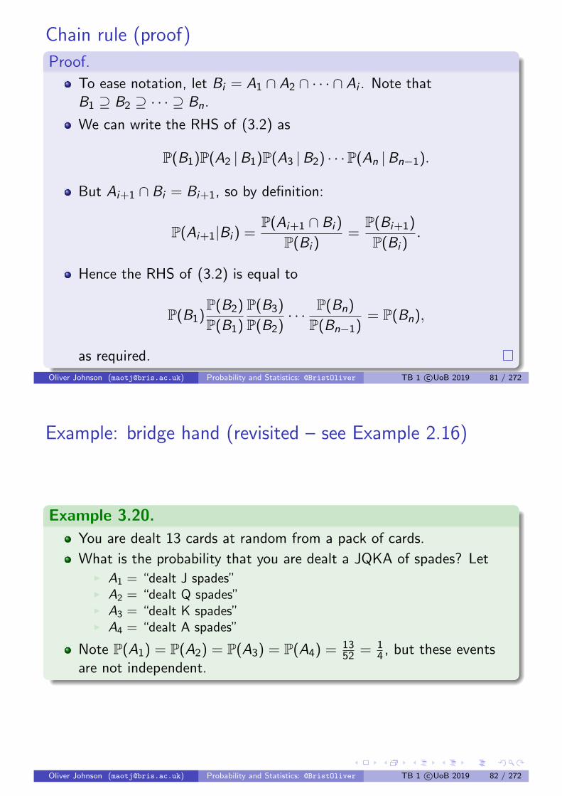
To ease notation, let Bi = A1 ∩ A2 ∩ · · · ∩ Ai . Note thatB1 ⊇ B2 ⊇ · · · ⊇ Bn.
We can write the RHS of (3.2) as
P(B1)P(A2 |B1)P(A3 |B2) · · ·P(An |Bn−1).
But Ai+1 ∩ Bi = Bi+1, so by definition:
P(Ai+1|Bi ) =P(Ai+1 ∩ Bi )
P(Bi )=
P(Bi+1)
P(Bi ).
Hence the RHS of (3.2) is equal to
P(B1)P(B2)
P(B1)
P(B3)
P(B2)· · · P(Bn)
P(Bn−1)= P(Bn),
as required.
Oliver Johnson ([email protected]) Probability and Statistics: @BristOliver TB 1 c©UoB 2019 81 / 272
Example: bridge hand (revisited – see Example 2.16)
Example 3.20.
You are dealt 13 cards at random from a pack of cards.
What is the probability that you are dealt a JQKA of spades? LetI A1 = “dealt J spades”I A2 = “dealt Q spades”I A3 = “dealt K spades”I A4 = “dealt A spades”
Note P(A1) = P(A2) = P(A3) = P(A4) = 1352 = 1
4 , but these eventsare not independent.
Oliver Johnson ([email protected]) Probability and Statistics: @BristOliver TB 1 c©UoB 2019 82 / 272

Example 3.20.
P(A2 |A1) =P(A1 ∩ A2)
P(A1)
=
(5011
)/(52
13
)(5112
)/(52
13
) (=
number of hands with J and Q
number of hands with J
)=
12
51(or see this directly?)
This is not equal to P(A2) = 14 .
Similarly P(A3 |A1 ∩ A2) = 1150 and P(A4 |A1 ∩ A2 ∩ A3) = 10
49 .
Deduce (as before) that
P(A1 ∩ A2 ∩ A3 ∩ A4)
= P(A1)P(A2 |A1)P(A3 |A1 ∩ A2)P(A4 |A1 ∩ A2 ∩ A3)
=13
52· 12
51· 11
50· 10
49.
Oliver Johnson ([email protected]) Probability and Statistics: @BristOliver TB 1 c©UoB 2019 83 / 272
Section 4: Discrete random variables
Objectives: by the end of this section you should be able to
To build a mathematical model for discrete random variablesTo understand the probability mass function, expectation andvariance of such variablesTo get experience in working with some of the basic distributions(Bernoulli, Binomial, Poisson, Geometric)
[The material for this Section is also covered in Chapter 4 of the coursebook.]
Oliver Johnson ([email protected]) Probability and Statistics: @BristOliver TB 1 c©UoB 2019 84 / 272

Section 4.1: Motivation and definitions
A trial selects an outcome ω from a sample space Ω.
Often we are interested in a number associated with the outcome.
Example 4.1.
Let ω be the positions of the stock market at the end of one day.
You are interested only in the amount of money you make.
That is a number that depends on the outcome ω.
Example 4.2.
Throw two fair dice. Look at the total score.
Let X (ω) be the total score when the outcome is ω.
Remember we write the sample space as
Ω = (a, b) : a, b = 1, . . . , 6.
So X ((a, b)) = a + b.
Oliver Johnson ([email protected]) Probability and Statistics: @BristOliver TB 1 c©UoB 2019 85 / 272
Formal definition
Definition 4.3.
Let Ω be a sample space.
A random variable (r.v.) X is a function X : Ω→ R.
That is, X assigns a value X (ω) to each outcome ω.
Remark 4.4.
For any set B ⊆ R, we use the notation P(X ∈ B) as shorthand for
P(ω ∈ Ω : X (ω) ∈ B).
E.g. X is the sum of the scores of two fair dice, P(X ≤ 3) isshorthand for
P(ω ∈ Ω : X (ω) ≤ 3) = P((1, 1), (1, 2), (2, 1)) =3
36.
Oliver Johnson ([email protected]) Probability and Statistics: @BristOliver TB 1 c©UoB 2019 86 / 272

Probability mass functionsIn this chapter we look at discrete random variables X , which arethose such that X (ω) takes a discrete set of values S = x1, x2, . . ..This avoids certain technicalities we will worry about in due course.
Definition 4.5.
Let X be a discrete r.v. taking values in S = x1, x2, . . ..The probability mass function (pmf) of X is the function pX given by
pX (x) = P(X = x) = P(ω ∈ Ω : X (ω) = x).
Remark 4.6.
If pX is a p.m.f. then
0 ≤ pX (x) ≤ 1 for all x∑x∈S pX (x) = 1 (since P(Ω) = 1).
In fact, any function with these properties can be thought of as a pmf ofsome random variable.Oliver Johnson ([email protected]) Probability and Statistics: @BristOliver TB 1 c©UoB 2019 87 / 272
Example 4.7.
X is the sum of the scores on 2 fair dice
x = 2 3 4 5 6 7 . . .
|ω : X (ω) = x| = 1 2 3 4 5 6 . . .
pX (x) = 136
236
336
436
536
636 . . .
x = 8 9 10 11 12
|ω : X (ω) = x| = 5 4 3 2 1
pX (x) = 536
436
336
236
136
Oliver Johnson ([email protected]) Probability and Statistics: @BristOliver TB 1 c©UoB 2019 88 / 272

Section 4.2: Bernoulli distribution
This is the building block for many distributions.
Named after Jakob Bernoulli, part of a very famous family ofmathematicians.
Definition 4.8.
Think of a trial with two outcomes: success or failure.
Ω = success, failure
This is called a Bernoulli trial.
Let X (failure) = 0 and X (success) = 1, so that X counts the numberof successes in the trial.
Suppose that P(success) = p, so thatP(failure) = 1− P(success) = 1− p.
Then we say that X has a Bernoulli distribution with parameter p.
Oliver Johnson ([email protected]) Probability and Statistics: @BristOliver TB 1 c©UoB 2019 89 / 272
Bernoulli distribution notation
Remark 4.9.
Notation: X ∼ Bernoulli(p)
X has pmf pX (0) = 1− p, pX (1) = p, pX (x) = 0 for x /∈ 0, 1.Equivalently, pX (x) = (1− p)1−xpx for x = 0, 1.
Oliver Johnson ([email protected]) Probability and Statistics: @BristOliver TB 1 c©UoB 2019 90 / 272

Example: Indicator functions
Example 4.10.
Let A be an event, and let random variable I be defined by
I (ω) =
1 ω ∈ A0 ω /∈ A
I is called the indicator function of A.
P(I = 1) = P(ω : I (ω) = 1) = P(A)P(I = 0) = P(ω : I (ω) = 0) = P(Ac)
That is pI (1) = P(A) and pI (0) = 1− P(A).
Thus I ∼ Bernoulli(P(A)).
Oliver Johnson ([email protected]) Probability and Statistics: @BristOliver TB 1 c©UoB 2019 91 / 272
Section 4.3: Binomial distribution
Definition 4.11.
Consider n independent Bernoulli trials
Each trial has probability p of success
Let T be the total number of successes
Then T is said to have a binomial distribution with parameters (n, p)
Notation: T ∼ Bin(n, p).
Oliver Johnson ([email protected]) Probability and Statistics: @BristOliver TB 1 c©UoB 2019 92 / 272

Binomial distribution example
Example 4.12.
Take n = 3 trials with p = 13
Ω = FFF ,FFS ,FSF ,SFF ,FSS ,SFS ,SSF ,SSS
P(FFF) =2
3· 2
3· 2
3=
8
27
P(FFS) = P(FSF) = P(SFF) =2
3· 2
3· 1
3=
4
27
P(FSS) = P(SFS) = P(SSF) =2
3· 1
3· 1
3=
2
27
P(SSS) =1
3· 1
3· 1
3=
1
27
Oliver Johnson ([email protected]) Probability and Statistics: @BristOliver TB 1 c©UoB 2019 93 / 272
Binomial distribution example (cont.)
Example 4.12.
HenceI T = 0 = FFF so that P(T = 0) = 8
27I T = 1 = FFS ,FSF ,SFF so that P(T = 1) = 3× 4
27 = 1227
I T = 2 = FSS ,SFS ,SSF so that P(T = 2) = 3× 227 = 6
27I T = 3 = SSS so that P(T = 3) = 1
27
Thus T has pmf
pT (0) =8
27, pT (1) =
12
27, pT (2) =
6
27, pT (3) =
1
27
with pT (x) = 0 otherwise.
Oliver Johnson ([email protected]) Probability and Statistics: @BristOliver TB 1 c©UoB 2019 94 / 272

General binomial distribution pmf
Lemma 4.13.
In general if T ∼ Bin(n, p) then
pT (x) = P(T = x) =
(n
x
)px(1− p)n−x , x = 0, 1, . . . , n.
Proof.
There are(nx
)sample points with x successes from the n trials.
Each of these sample points has probability px(1− p)n−x .
Exercise: Verify that∑n
x=0 pX (x) = 1 in this case (Hint: use Proposition2.12.3).
Oliver Johnson ([email protected]) Probability and Statistics: @BristOliver TB 1 c©UoB 2019 95 / 272
Binomial distribution example
Example 4.14.
40% of a large population vote Labour.
A random sample of 10 people is taken.
What is the probability that not more than 2 people vote Labour?
Let T be the number of people that vote Labour. SoT ∼ Bin(10, 0.4).
P(T ≤ 2) = pT (0) + pT (1) + pT (2)
=
(10
0
)(0.4)0(0.6)10 +
(10
1
)(0.4)1(0.6)9
+
(10
2
)(0.4)2(0.6)8
= 0.167
Oliver Johnson ([email protected]) Probability and Statistics: @BristOliver TB 1 c©UoB 2019 96 / 272

Section 4.4: Geometric distribution
Definition 4.15.
Carry out independent Bernoulli trials until we obtain first success.
Let X be the number of the trial when we see the first success.
Suppose the probability of a success on any one trial is p, then
P(X = x) = (1− p)x−1p, x = 1, 2, 3, . . .
Hence the mass function is
pX (x) = P(X = x) = p(1− p)x−1, x = 1, 2, 3, . . .
with pX (x) = 0 otherwise.
X is said to have a geometric distribution with parameter p
Notation: X ∼ Geom(p)
Exercise: Verify that∑∞
x=1 pX (x) = 1.
Oliver Johnson ([email protected]) Probability and Statistics: @BristOliver TB 1 c©UoB 2019 97 / 272
Example: call-centre
Example 4.16.
Consider a call-centre which has 10 incoming phone lines.
Each time an operative is free, they answer a random line.
Let X be the number of people served (up to and including yourself)from the time that you get through.
Each time the operative serves someone there is a probability 110 that
it will be you.
So X ∼ Geom( 110 ).
x = 1 2 3 4 5 6 · · ·P(X = x) = 0.1 0.09 0.081 0.0729 0.06561 0.059049 · · ·
Oliver Johnson ([email protected]) Probability and Statistics: @BristOliver TB 1 c©UoB 2019 98 / 272

Geometric tail distribution
Lemma 4.17.
If X ∼ Geom(p) then P(X > x) = (1− p)x for any integer x ≥ 0.
Proof.
Write q = 1− p. Then
P(X > x) = P(X = x + 1) + P(X = x + 2) + P(X = x + 3) + · · ·= pqx + pqx+1 + pqx+2 + · · ·= pqx(1 + q + q2 + · · · )
= pqx1
1− q
= pqx1
p
= qx
by summing a geometric progression to infinity.Oliver Johnson ([email protected]) Probability and Statistics: @BristOliver TB 1 c©UoB 2019 99 / 272
Waiting time formulation
Remark 4.18.
Lemma 4.17 is easily seen by thinking about waiting for successes: theprobability of waiting more than x for a success is the probability that youget failures on the first x trials, which has probability (1− p)x .
If waiting at the call-centre (Example 4.16),
P(X > 10) = 0.910 = 0.349 (to 3 s.f.).
Oliver Johnson ([email protected]) Probability and Statistics: @BristOliver TB 1 c©UoB 2019 100 / 272

Lack-of-memory property
Lemma 4.19.
Lack of memory property If X ∼ Geom(p) then for any x ≥ 1:
P(X = x + n |X > n) = P(X = x).
Remark 4.20.
In the call-centre example (Example 4.16) this tells us for examplethat
P(X = 5 + x |X > 5) = P(X = x).
The fact that you have waited for 5 other people to get serveddoesn’t mean you are more likely to get served quickly than if youhave just joined the queue.
Oliver Johnson ([email protected]) Probability and Statistics: @BristOliver TB 1 c©UoB 2019 101 / 272
Section 4.5: Poisson distribution
Definition 4.21.
Let λ > 0 be a real number.
A r.v. X has a Poisson distribution with parameter λ if X takesvalues in the range 0,1,2,. . . and has pmf
pX (x) = e−λλx
x!, x = 0, 1, 2, . . . .
Notation: X ∼ Poi(λ).
Exercise: verify that∑∞
x=0 pX (x) = 1.
Hint: see later in Analysis that
∞∑x=0
λx
x!= eλ.
Oliver Johnson ([email protected]) Probability and Statistics: @BristOliver TB 1 c©UoB 2019 102 / 272

Two motivations
Remark 4.22.
If X ∼ Bin(n, p) with n large and p small then
P(X = x) ≈ e−np(np)x
x!
i.e. X is distributed approximately the same as a Poi(λ) random variablewhere λ = np.
Remark 4.23.
In the second year Probability 2 course you can see that the Poissondistribution is a natural distribution for the number of arrivals ofsomething in a given time period: telephone calls, internet traffic, diseaseincidences, nuclear particles.
Oliver Johnson ([email protected]) Probability and Statistics: @BristOliver TB 1 c©UoB 2019 103 / 272
Example: airline tickets
Example 4.24.
An airline sells 403 tickets for a flight with 400 seats.
On average 1% of purchasers fail to turn up.
What is the probability that there are more passengers than seats(someone is bumped)?
Let X = number of purchasers that fail to turn up.
True distribution X ∼ Bin(403, 0.01)
Approximately X ∼ Poi(4.03)
Oliver Johnson ([email protected]) Probability and Statistics: @BristOliver TB 1 c©UoB 2019 104 / 272

Example: airline tickets (cont.)
Example 4.24.
P(X = x) ≈ e−4.03 4.03x
x!
x = 0 1 2 3 4 5 · · ·P(X = x) ≈ 0.0178 0.0716 0.144 0.1939 0.1953 0.1574 · · ·
We can deduce that
P(at least one passenger bumped)
= P(X ≤ 2) = pX (0) + pX (1) + pX (2)
≈ 0.2334.
Oliver Johnson ([email protected]) Probability and Statistics: @BristOliver TB 1 c©UoB 2019 105 / 272
Section 5: Expectation and variance
Objectives: by the end of this section you should be able to
To understand where random variables are centred and howdispersed they areTo understand basic properties of mean and varianceTo use results such as Chebyshev’s theorem to bound probabilities
[The material for this Section is also covered in Chapter 4 of the coursebook.]
Oliver Johnson ([email protected]) Probability and Statistics: @BristOliver TB 1 c©UoB 2019 106 / 272

Section 5.1: Expectation
We want some concept of the average value of a r.v. X and thespread about this average.
Some of this will seem slightly arbitrary for now, but we will provesome results that help motivate why it is convenient to make thesedefinitions after we have introduced jointly-distributed r.v.s.
Definition 5.1.
Let X be a random variable taking the values in a discrete set S .
The expected value (or expectation) of X , denoted E(X ), is defined as
E(X ) =∑x∈S
xpX (x).
This is well-defined so long as∑
x∈S |x |pX (x) converges.
Oliver Johnson ([email protected]) Probability and Statistics: @BristOliver TB 1 c©UoB 2019 107 / 272
Example
Remark 5.2.
E(X ) is also sometimes called the mean of the distribution of X .
Example 5.3.
Consider a Bernoulli random variable.
Recall from Remark 4.9 that if X ∼ Bernoulli(p) then X has pmfpX (0) = 1− p, pX (1) = p, pX (x) = 0 for x /∈ 0, 1.Hence in Definition 5.1
E(X ) = 0 · (1− p) + 1 · p = p.
Note that for p 6= 0, 1 this random variable X won’t ever equal E(X ).
Oliver Johnson ([email protected]) Probability and Statistics: @BristOliver TB 1 c©UoB 2019 108 / 272

Motivation
Remark 5.4.
Do not confuse E(X ) with the the mean of a collection of observedvalues, which is referred to as the sample mean.
However, there is a relationship between E(X ) and sample meanwhich motivates the definition.
Perform an experiment and observe the random variable X whichtakes values in the discrete set S .
Repeat the experiment infinitely often, and observe outcomes X1, X2,. . .
Consider the limit of the sample means
limn→∞
X1 + · · ·+ Xn
n.
Oliver Johnson ([email protected]) Probability and Statistics: @BristOliver TB 1 c©UoB 2019 109 / 272
Motivation (cont.)
Remark 5.5.
Let an(x) be the number of times the outcome is x in the first ntrials. Then reordering the sum, we know that
X1 + X2 + · · ·+ Xn =∑x∈S
xan(x).
We expect (but have not yet proved) that
an(x)
n→ pX (x) as n→∞.
If so then
X1 + · · ·+ Xn
n=
∑x∈S xan(x)
n=∑x∈S
xan(x)
n→∑x∈S
xpX (x).
This motivates Definition 5.1.
Oliver Johnson ([email protected]) Probability and Statistics: @BristOliver TB 1 c©UoB 2019 110 / 272

Section 5.2: Examples
Example 5.6 (Uniform random variable).
Let X take the integer values 1, . . . , n.
pX (x) =
1n x = 1, . . . , n0 otherwise
E(X ) =n∑
x=1
x1
n=
1
n
n∑x=1
x =1
n
1
2n(n + 1) =
n + 1
2.
Hence for example if n = 6, the expected value of a dice roll is 7/2.
Oliver Johnson ([email protected]) Probability and Statistics: @BristOliver TB 1 c©UoB 2019 111 / 272
Example: binomial distribution
Example 5.7.
X ∼ Bin(n, p) (see Definition 4.11).
P(X = x) =
(nx
)px(1− p)n−x x = 0, 1, . . . , n
0 otherwise
E(X ) =n∑
x=0
x
(n
x
)px(1− p)n−x
= npn∑
x=1
(n − 1
x − 1
)px−1(1− p)(n−1)−(x−1)
= np.
Here we use the fact that x(nx
)= n
(n−1x−1
)(check directly?) and apply
the Binomial Theorem 2.12.3.
There are easier ways — see later.
Oliver Johnson ([email protected]) Probability and Statistics: @BristOliver TB 1 c©UoB 2019 112 / 272
Example: Poisson distribution
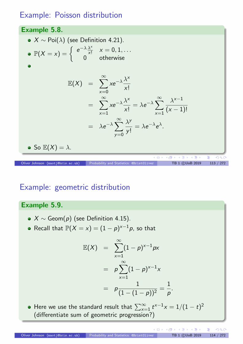
Example 5.8.
X ∼ Poi(λ) (see Definition 4.21).
P(X = x) =
e−λ λ
x
x! x = 0, 1, . . .0 otherwise
E(X ) =∞∑x=0
xe−λλx
x!
=∞∑x=1
xe−λλx
x!= λe−λ
∞∑x=1
λx−1
(x − 1)!
= λe−λ∞∑y=0
λy
y != λe−λeλ.
So E(X ) = λ.
Oliver Johnson ([email protected]) Probability and Statistics: @BristOliver TB 1 c©UoB 2019 113 / 272
Example: geometric distribution
Example 5.9.
X ∼ Geom(p) (see Definition 4.15).
Recall that P(X = x) = (1− p)x−1p, so that
E(X ) =∞∑x=1
(1− p)x−1px
= p∞∑x=1
(1− p)x−1x
= p1
(1− (1− p))2=
1
p.
Here we use the standard result that∑∞
x=1 tx−1x = 1/(1− t)2
(differentiate sum of geometric progression?)
Oliver Johnson ([email protected]) Probability and Statistics: @BristOliver TB 1 c©UoB 2019 114 / 272

Section 5.3: Expectation of a function of a r.v.
Consider a random variable X taking values x1, x2, . . .
Take a function g : R→ R.
Define a new r.v. Z (ω) = g(X (ω)).
Then Z takes values in the range z1 = g(x1), z2 = g(x2). . . .
Look at E(Z ).
By definition E(Z ) =∑
i zipZ (zi ) where pZ is the pmf of Z which wecould in principle work out.
But it’s often easier to use
Theorem 5.10.
Let Z = g(X ). Then
E(Z ) =∑i
g(xi )pX (xi ) =∑x∈S
g(x)pX (x).
Oliver Johnson ([email protected]) Probability and Statistics: @BristOliver TB 1 c©UoB 2019 115 / 272
Proof.
(you are not required to know this proof)
Recall that pZ (zi ) = P(Z = zi ) = P(ω ∈ Ω : Z (ω) = zi).Notice that
ω ∈ Ω : Z (ω) = zi =⋃
j : g(xj )=zi
ω : X (ω) = xj,
which is a disjoint union.So pZ (zi ) =
∑j : g(xj )=zi
pX (xj).Therefore
E(Z ) =∑i
zipZ (zi ) =∑i
zi
∑j : g(xj )=zi
pX (xj)
=
∑i
∑j : g(xj )=zi
g(xj)pX (xj)
=∑j
g(xj)pX (xj).
Oliver Johnson ([email protected]) Probability and Statistics: @BristOliver TB 1 c©UoB 2019 116 / 272

Example 5.11.
Returning to Example 5.6:
pX (x) =
1n x = 1, . . . , n0 otherwise
Consider Z = X 2 so Z takes the values 1, 4, 9, . . . , n2 each withprobability 1
n . We have g(x) = x2.
By Theorem 5.10
E(Z ) =n∑
x=1
g(x)pX (x)
=n∑
x=1
x2 1
n=
1
n
n∑x=1
x2
=1
n
1
6n(n + 1)(2n + 1) =
1
6(n + 1)(2n + 1)
Oliver Johnson ([email protected]) Probability and Statistics: @BristOliver TB 1 c©UoB 2019 117 / 272
Linearity of expectation
Lemma 5.12.
Let a and b be constants. Then E(aX + b) = aE(X ) + b.
Proof.
Let g(x) = ax + b. From Theorem 5.10 we know that
E(g(X )) =∑i
g(xi )pX (xi ) =∑i
(axi + b)pX (xi )
= a∑i
xipX (xi ) + b∑i
pX (xi ) = aE(X ) + b.
Oliver Johnson ([email protected]) Probability and Statistics: @BristOliver TB 1 c©UoB 2019 118 / 272

Section 5.4: Variance
This is the standard measure for the spread of a distribution.
Definition 5.13.
Let X be a r.v., and let µ = E(X ).
Define the variance of X , denoted by Var (X ), by
Var (X ) = E((X − µ)2
).
Notation: Var (X ) is often denoted σ2.
The standard deviation of X is√Var (X ).
Oliver Johnson ([email protected]) Probability and Statistics: @BristOliver TB 1 c©UoB 2019 119 / 272
Example of spread
Example 5.14.
Define
Y =
1, wp.
1
2,
−1, wp.1
2,
U =
10, wp.
1
2,
−10, wp.1
2,
Z =
2, wp.
1
5,
−1
2, wp.
4
5.
Notice EY = EZ = EU = 0, the expectation does not distinguishbetween these rv.’s.
Yet they are clearly different, and the variance helps capture this.
Var (Y ) = E(Y − 0)2 = 12 · 1
2+ (−1)2 · 1
2= 1,
Var (U) = E(U − 0)2 = 102 · 1
2+ (−10)2 · 1
2= 100,
Var (Z ) = E(Z − 0)2 = 22 · 1
5+(−1
2
)2· 4
5= 1.
Oliver Johnson ([email protected]) Probability and Statistics: @BristOliver TB 1 c©UoB 2019 120 / 272

Useful lemma
Lemma 5.15.
Var (X ) = E(X 2)− (E(X ))2
Sketch proof: see Theorem 7.14.
Var (X ) = E((X − µ)2)
= E(X 2 − 2µX + µ2)
= E(X 2)− 2µE(X ) + µ2 (will prove this step later)
= E(X 2)− 2µ2 + µ2
= E(X 2)− µ2
Oliver Johnson ([email protected]) Probability and Statistics: @BristOliver TB 1 c©UoB 2019 121 / 272
Example: Bernoulli random variable
Example 5.16.
Recall from Remark 4.9 and Example 5.3 that if X ∼ Bernoulli(p)then pX (0) = 1− p, pX (1) = p and EX = p.
We can calculate Var (X ) in two different ways:1 Var (X ) = E(X − µ)2 =
∑x pX (x)(x − p)2 =
(1− p)(−p)2 + p(1− p)2 = (1− p)p(p + 1− p) = p(1− p).2 Alternatively:
E(X 2) =∑x
pX (x)x2 = (1− p)02 + p12 = p,
so that Var (X ) = E(X 2)− (EX )2 = p − p2 = p(1− p).
Remark 5.17.
We will see in Example 7.17 below that if X ∼ Bin(n, p) (see Definition4.11) then Var (X ) = np(1− p). (Need to know this formula)
Oliver Johnson ([email protected]) Probability and Statistics: @BristOliver TB 1 c©UoB 2019 122 / 272

Uniform Example
Example 5.18.
Again consider the uniform random variable (from Example 5.6)
pX (x) =
1n x = 1, . . . , n0 otherwise
Know from Example 5.6 that E(X ) = n+12 and from Example 5.11
that E(X 2) = 16 (n + 1)(2n + 1).
Thus
Var (X ) =1
6(n + 1)(2n + 1)−
(n + 1
2
)2
=n + 1
12(4n + 2− 3(n + 1))
=(n + 1)
12(n − 1) =
(n2 − 1)
12.
Oliver Johnson ([email protected]) Probability and Statistics: @BristOliver TB 1 c©UoB 2019 123 / 272
Example: Poisson random variable
Example 5.19.
Consider X ∼ Poi(λ) (see Definition 4.21).
Recall that P(X = x) =
e−λ λ
x
x! x = 0, 1, . . .0 otherwise
and E(X ) = λ.
We show (see next page) that E(X 2) = λ2 + λ.
Thus Var (X ) = E(X 2)− (E(X ))2 = (λ2 + λ)− (λ)2 = λ.
Oliver Johnson ([email protected]) Probability and Statistics: @BristOliver TB 1 c©UoB 2019 124 / 272

Example: Poisson (cont.)
Example 5.19.
Key is that x2 = x(x − 1) + x , so again changing the range of summation:
E(X 2) =∞∑x=0
x2e−λλx
x!
=∞∑x=0
x(x − 1)e−λλx
x!+∞∑x=0
xe−λλx
x!
= λ2e−λ∞∑x=2
λx−2
(x − 2)!+ λe−λ
∞∑x=1
λx−1
(x − 1)!
= λ2e−λ
( ∞∑z=0
λz
z!
)+ λe−λ
∞∑y=0
λy
y !
= λ2 + λ,
since each bracketed term is precisely eλ as before.Oliver Johnson ([email protected]) Probability and Statistics: @BristOliver TB 1 c©UoB 2019 125 / 272
Non-linearity of variance
We now state (and prove later) an important result concerning variances,which is the counterpart of Lemma 5.12:
Lemma 5.20.
Let a and b be constants. Then Var (aX + b) = a2Var (X ).
Oliver Johnson ([email protected]) Probability and Statistics: @BristOliver TB 1 c©UoB 2019 126 / 272

Section 5.5: Chebyshev’s inequality
Let X be any random variable with finite mean µ and variance σ2,and let c be any constant.
Define the indicator variable I (ω) =
1 if |X (ω)− µ| > c0 otherwise
CalculateE(I ) = 0 · P(I = 0) + 1 · P(I = 1) = P(I = 1) = P(|X − µ| > c).
Define also Z (ω) = (X (ω)− µ)2/c2, so that
E(Z ) = E(
(X − µ)2
c2
)=
E((X − µ)2)
c2=σ2
c2
This last step uses Lemma 5.12 with a = 1/c2 and b = 0.
Notice that I (ω) ≤ Z (ω) for any ω. (plot a graph?)
So E(I ) ≤ E(Z ), and we deduce that . . .
Oliver Johnson ([email protected]) Probability and Statistics: @BristOliver TB 1 c©UoB 2019 127 / 272
Theorem 5.21 (Chebyshev’s inequality).
For any random variable X with finite mean µ and variance σ2, and anyconstant c :
P(|X − µ| > c) ≤ σ2
c2.
Remark 5.22.
We have not made any assumptions about the distribution of X(other than finite mean and variance)
We have shown that the probability that X is further than someconstant from µ is bounded by some quantity that increases with thevariance σ2 and decreases with the distance from µ.
This shows that the axioms and definitions we have made give ussomething that at least fits with our intuition.
Oliver Johnson ([email protected]) Probability and Statistics: @BristOliver TB 1 c©UoB 2019 128 / 272

Application of Chebyshev’s inequality
Example 5.23.
A fair coin is tossed 104 times.Let T denote the total number of heads.Then since T ∼ Bin(104, 0.5) we have E(T ) = 5000 andVar (T ) = 2500 (see Example 5.7 and Remark 5.17).Thus by taking c = 500 in Chebyshev’s inequality (Theorem 5.21) wehave
P(|T − 5000| > 500) ≤ 0.01,
so thatP(4500 ≤ T ≤ 5500) ≥ 0.99.
We can also express this as
P(
0.45 ≤ T
104≤ 0.55
)≥ 0.99.
Oliver Johnson ([email protected]) Probability and Statistics: @BristOliver TB 1 c©UoB 2019 129 / 272
Section 6: Joint distributions
Objectives: by the end of this section you should be able to
Understand the joint probability mass functionKnow how to use relationships between joint, marginal andconditional probability mass functionsUse convolutions to calculate mass functions of sums.
[This material is also covered in Chapter 6 of the course book.]
Oliver Johnson ([email protected]) Probability and Statistics: @BristOliver TB 1 c©UoB 2019 130 / 272

Section 6.1: The joint probability mass function
Up to now we have only considered a single random variable at once,but now consider related random variables.
Often we want to measure two attributes, X and Y , in the sameexperiment.
For exampleI height X and weight Y of a randomly chosen personI the DNA profile X and the cancer type Y of a randomly chosen person.
Oliver Johnson ([email protected]) Probability and Statistics: @BristOliver TB 1 c©UoB 2019 131 / 272
Joint probability mass function
Recall that random variables are functions of the underlying outcomeω in sample space Ω.
Hence two random variables are simply two different functions of ω inthe same sample space.
In particular, consider discrete random variables X ,Y : Ω 7→ R.
Definition 6.1.
The joint pmf for X and Y is pX ,Y , defined by
pX ,Y (x , y) = P(X = x ,Y = y)
= P(ω : X (ω) = x ∩ ω : Y (ω) = y
)We can define the joint pmf of random variables X1, . . . ,Xn in ananalogous way.
Oliver Johnson ([email protected]) Probability and Statistics: @BristOliver TB 1 c©UoB 2019 132 / 272
Example: coin tosses
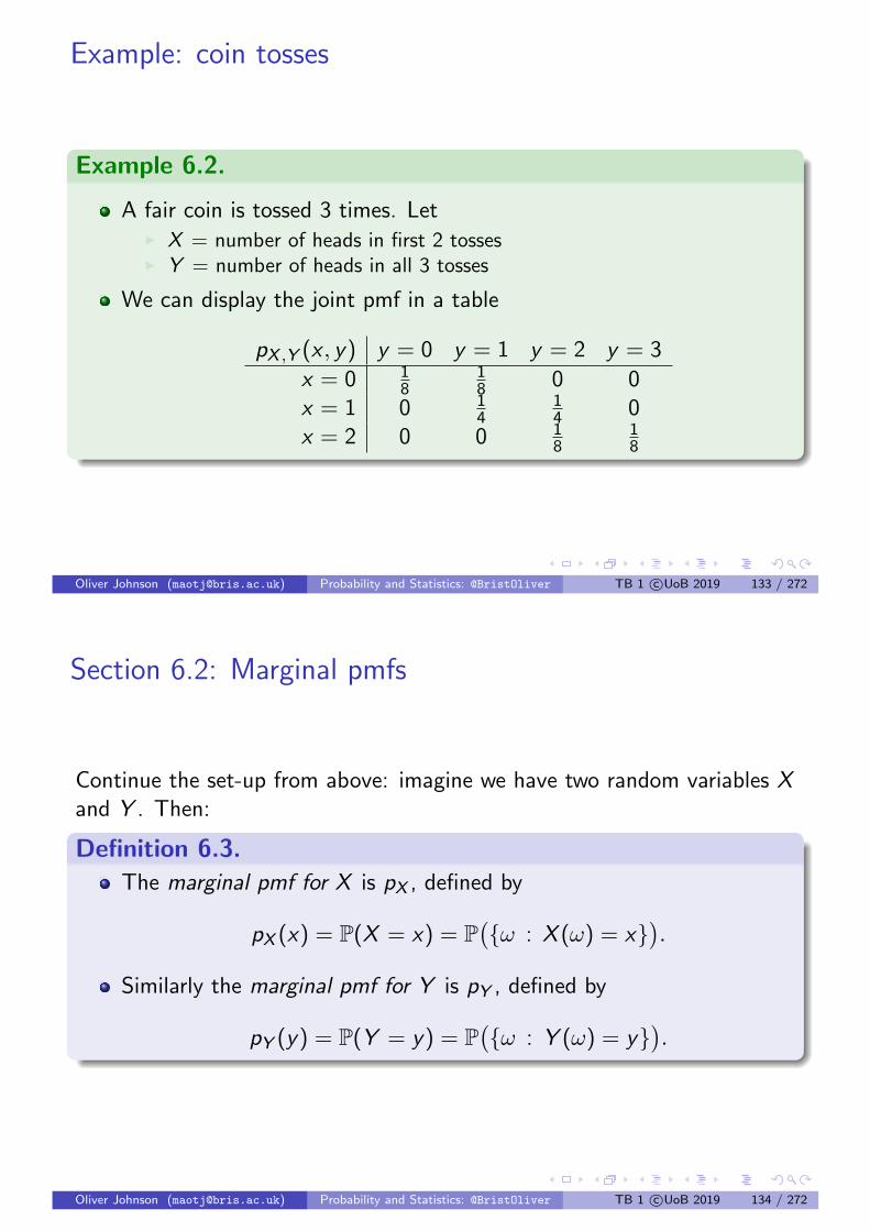
Example 6.2.
A fair coin is tossed 3 times. LetI X = number of heads in first 2 tossesI Y = number of heads in all 3 tosses
We can display the joint pmf in a table
pX ,Y (x , y) y = 0 y = 1 y = 2 y = 3
x = 0 18
18 0 0
x = 1 0 14
14 0
x = 2 0 0 18
18
Oliver Johnson ([email protected]) Probability and Statistics: @BristOliver TB 1 c©UoB 2019 133 / 272
Section 6.2: Marginal pmfs
Continue the set-up from above: imagine we have two random variables Xand Y . Then:
Definition 6.3.
The marginal pmf for X is pX , defined by
pX (x) = P(X = x) = P(ω : X (ω) = x
).
Similarly the marginal pmf for Y is pY , defined by
pY (y) = P(Y = y) = P(ω : Y (ω) = y
).
Oliver Johnson ([email protected]) Probability and Statistics: @BristOliver TB 1 c©UoB 2019 134 / 272

Joint pmf determines the marginalsSuppose X takes values x1, x2, . . . and Y takes values y1, y2, . . ..Then for each xi :
X = xi =⋃j
X = xi ,Y = yj (disjoint union),
=⇒ P(X = xi ) =∑j
P(X = xi ,Y = yj) (Axiom 3).
Hence (and with a corresponding argument for Y = yj) we deducethat summing over the joint distribution determines the marginals:
Theorem 6.4.
For any random variables X and Y :
pX (xi ) =∑j
pX ,Y (xi , yj)
pY (yj) =∑i
pX ,Y (xi , yj),
Oliver Johnson ([email protected]) Probability and Statistics: @BristOliver TB 1 c©UoB 2019 135 / 272
Example: coin tosses (return to Example 6.2)
Example 6.5.
A fair coin is tossed 3 times. LetI X = number of heads in first 2 tossesI Y = number of heads in all 3 tosses
We can display the joint and marginal pmfs in a table
pX ,Y (x , y) y = 0 y = 1 y = 2 y = 3
x = 0 18
18 0 0 1
4x = 1 0 1
414 0 1
2x = 2 0 0 1
818
14
18
38
38
18
We calculate marginals for X by summing the rows of the table.
We calculate marginals for Y by summing the columns.
Oliver Johnson ([email protected]) Probability and Statistics: @BristOliver TB 1 c©UoB 2019 136 / 272

Marginal pmfs don’t determine joint
Example 6.6.
Consider tossing a fair coin once.
Let X be the number of heads, and let Y be the number of tails.
Write the joint pmf in a table:
pX ,Y (x , y) y = 0 y = 1
x = 0 0 12
x = 1 12 0
Either write down the marginals directly, or calculate
pX (0) = pX ,Y (0, 0) + pX ,Y (0, 1) =1
2,
and pX (1) = 1− pX (0) = 12 and similarly pY (0) = pY (1) = 1
2 .
Oliver Johnson ([email protected]) Probability and Statistics: @BristOliver TB 1 c©UoB 2019 137 / 272
Marginal pmfs don’t determine joint (cont.)
Example 6.7.
Now toss a fair coin twice.
Let X is the number of heads on the first throw, and Y be thenumber of tails on the second throw.
Write the joint pmf in a table:
pX ,Y (x , y) y = 0 y = 1
x = 0 14
14
x = 1 14
14
Summing rows and columns we see thatpX (0) = pX (1) = pY (0) = pY (1) = 1
2 , just as in Example 6.6.
Comparing Examples 6.6 and 6.7 we see that the marginal pmfs don’tdetermine the joint pmf.
Oliver Johnson ([email protected]) Probability and Statistics: @BristOliver TB 1 c©UoB 2019 138 / 272

Section 6.3: Conditional pmfs
Definition 6.8.
The conditional pmf for X given Y = y is pX |Y , defined by
pX |Y (x |y) = P(X = x |Y = y).
(This is only well-defined for y for which P(Y = y) > 0.)
Similarly the conditional pmf for Y given X = x is pY |X , defined by
pY |X (y |x) = P(Y = y |X = x).
Oliver Johnson ([email protected]) Probability and Statistics: @BristOliver TB 1 c©UoB 2019 139 / 272
Calculating conditional pmfs
Remark 6.9.
Notice that
pX |Y (x |y) = P(X = x |Y = y) =P(X = x ,Y = y)
P(Y = y)
=pX ,Y (x , y)
pY (y). (6.1)
Similarly
pY |X (y |x) =pX ,Y (x , y)
pX (x).
Oliver Johnson ([email protected]) Probability and Statistics: @BristOliver TB 1 c©UoB 2019 140 / 272

Conditional pmfs are probability mass functions
Remark 6.10.
We can check (in the spirit of Remark 4.6) that for any fixed y, thepX |Y (· | y) is a pmf.
That is, for any x , since (6.1) expresses it as a ratio of probabilities,clearly pX |Y (· | y) ≥ 0.
Similarly using Theorem 6.4 we know that pY (y) =∑
x pX ,Y (x , y).
This means that (by (6.1))∑x
pX |Y (x | y) =∑x
pX ,Y (x , y)
pY (y)
=1
pY (y)
∑x
pX ,Y (x , y) =1
pY (y)pY (y) = 1,
as required.
Oliver Johnson ([email protected]) Probability and Statistics: @BristOliver TB 1 c©UoB 2019 141 / 272
Example 6.2 continued
Example 6.11.
Condition on X = 2:
pY |X (y |2) =pX ,Y (2, y)
pX (2)= 4pX ,Y (2, y)
y 0 1 2 3
pY |X (y |2) 0 0 12
12
Condition on Y = 1
pX |Y (x |1) =pX ,Y (x , 1)
pY (1)=
8
3pX ,Y (x , 1)
x 0 1 2
pX |Y (x |1) 13
23 0
Oliver Johnson ([email protected]) Probability and Statistics: @BristOliver TB 1 c©UoB 2019 142 / 272

Example: Inviting friends to the pub
Example 6.12.
You decide to invite every friend you see today to the pub tonight.
You have 3 friends (!)
You will see each of them with probability 12 .
Each invited friend will come with probability 23 independently of the
others.
Find the distribution of the number of friends you meet in the pub.
Let X be the number of friends you invite.
X ∼ Bin(3, 12 ) so pX (x) =
(3x
) (12
)x (12
)3−x=(3x
)18 for 0 ≤ x ≤ 3.
Let Y be the number of friends who come to the pub.
Y |X = x ∼ Bin(x , 23 ) so pY |X (y |x) =
(xy
) (23
)y (13
)x−yfor 0 ≤ y ≤ x .
Oliver Johnson ([email protected]) Probability and Statistics: @BristOliver TB 1 c©UoB 2019 143 / 272
Example: Inviting friends to the pub (cont.)
Example 6.12.
So pX ,Y (x , y) = pX (x)pY |X (y |x) =
18
(3x
)(xy
)2y
3x 0 ≤ y ≤ x ≤ 3
0 otherwise
y = 0 1 2 3
x = 0 18 × 1 = 1
8 0 0 01 3
8 ×13 = 1
838 ×
23 = 1
4 0 02 3
8 ×19 = 1
2438 ×
49 = 1
638 ×
49 = 1
6 03 1
8 ×1
27 = 1216
18 ×
627 = 1
3618 ×
1227 = 1
1818 ×
827 = 1
27
827
1227
627
127
Therefore E(Y ) = 0× 827 + 1× 12
27 + 2× 627 + 3× 1
27 = 12+12+327 = 1.
There is a much easier way to calculate E(Y ) - see Section 10.
Oliver Johnson ([email protected]) Probability and Statistics: @BristOliver TB 1 c©UoB 2019 144 / 272

Section 6.4: Independent random variables
Definition 6.13.
Two random variables are independent if
pX ,Y (x , y) = pX (x)pY (y), for all x and y .
In general, random variables X1, . . . ,Xn are independent if
pX1,...,Xn(x1, . . . , xn) =n∏
i=1
pXi(xi ), for all xi .
Oliver Johnson ([email protected]) Probability and Statistics: @BristOliver TB 1 c©UoB 2019 145 / 272
Properties of independent random variables
Remark 6.14.
1 Consistent with Definition 3.16 (independence of events).
2 We require that the events X = x and Y = y are independentfor any x and y .
3 In fact this is equivalent to requiring events X ∈ A and Y ∈ Bindependent for any A and B.
4 Important: if X and Y are independent, so are g(X ) and h(Y ) forany functions g and h. a
aProof (not examinable): For any u, v
P(g(X ) = u, h(Y ) = v) = P(X ∈ g−1(u)
⋂Y ∈ h−1(v)
)= P
(X ∈ g−1(u)
)P(⋂
Y ∈ h−1(v))
= P(g(X ) = u)P(h(Y ) = v).
Oliver Johnson ([email protected]) Probability and Statistics: @BristOliver TB 1 c©UoB 2019 146 / 272

IID random variables
Definition 6.15.
We say that random variables X1, . . . ,Xn are IID (independent andidentically distributed) if they are independent, and all their marginalspXi
are the same, so
pX1,...,Xn(x1, . . . , xn) =n∏
i=1
pX (xi ),
for some fixed pX .
Here we obtain marginals pX1(x1) =∑
x2,...,xnpX1,...,Xn(x1, . . . , xn) etc.
Oliver Johnson ([email protected]) Probability and Statistics: @BristOliver TB 1 c©UoB 2019 147 / 272
Example
Example 6.16.
Again return to Example 1.2, rolling red and green dice.
Let X be the number on the red dice, Y on the green dice.
Then every pair of numbers have equal probability:
pX ,Y (x , y) =1
36=
1
6· 1
6= pX (x) · pY (y) for all x , y = 1, . . . , 6.
We see that these variables are independent (in fact IID as well).
Oliver Johnson ([email protected]) Probability and Statistics: @BristOliver TB 1 c©UoB 2019 148 / 272

Discrete convolution
Proposition 6.17.
Let X and Y be independent, integer valued random variables withrespective mass functions pX and pY . Then
pX+Y (k) =∞∑
i=−∞pX (k − i) · pY (i), for all k ∈ Z.
This formula is called the discrete convolution of the mass functions pXand pY .
Oliver Johnson ([email protected]) Probability and Statistics: @BristOliver TB 1 c©UoB 2019 149 / 272
Discrete convolution proof
Proof.
Using independence, and since it is a disjoint union, we know that
pX+Y (k) = P(X + Y = k) = P
( ∞⋃i=−∞
X + Y = k ,Y = i
)
=∞∑
i=−∞P(X + Y = k , Y = i)
=∞∑
i=−∞P(X = k − i , Y = i) =
∞∑i=−∞
P(X = k − i)P(Y = i)
=∞∑
i=−∞pX (k − i) · pY (i).
Oliver Johnson ([email protected]) Probability and Statistics: @BristOliver TB 1 c©UoB 2019 150 / 272

Convolution of Poissons gives a Poisson
Theorem 6.18.
Recall the definition of the Poisson distribution from Definition 4.21.
Let X ∼ Poi(λ) and Y ∼ Poi(µ) be independent.
Then X + Y ∼ Poi(λ+ µ).
Oliver Johnson ([email protected]) Probability and Statistics: @BristOliver TB 1 c©UoB 2019 151 / 272
Proof of Theorem 6.18
Proof.
Using Proposition 6.17, since X and Y only take positive values we know
pX+Y (k) =k∑
i=0
pX (k − i)pY (i)
=k∑
i=0
(e−λ
λk−i
(k − i)!
)(e−µ
µi
i !
)
= e−(λ+µ) 1
k!
k∑i=0
(k
i
)λk−iµi
= e−(λ+µ) (λ+ µ)k
k!,
where we use the Binomial Theorem, Proposition 2.12.3.
Oliver Johnson ([email protected]) Probability and Statistics: @BristOliver TB 1 c©UoB 2019 152 / 272

Section 7: Properties of mean and variance
Objectives: by the end of this section you should be able to
To explore further properties of expectations of a single andmultiple variables.To understand and use the Law of Large Numbers.To define covariance, and use it for computing variances of sums.To calculate and interpret correlation coefficients.
[This material is also covered in Sections 7.1 to 7.3 of the course book]
Oliver Johnson ([email protected]) Probability and Statistics: @BristOliver TB 1 c©UoB 2019 153 / 272
Section 7.1: Properties of expectation E
Theorem 7.1.
1 Let X be a constant r.v. with P(X = c) = 1. Then E(X ) = c .
2 Let a and b be constants and X be a r.v. ThenE(aX + b) = aE(X ) + b.
3 Let X and Y be r.v.s. Then E(X + Y ) = E(X ) + E(Y ).
Proof.1 If P(X = c) = 1 then E(X ) = cP(X = c) = c.
2 This is Lemma 5.12.
Oliver Johnson ([email protected]) Probability and Statistics: @BristOliver TB 1 c©UoB 2019 154 / 272

Proof of Theorem 7.1 (cont).
Proof.3 Let Z = X + Y , i.e. Z = g(X ,Y ) where g(x , y) = x + y .Then
E(Z ) =∑xi
∑yj
g(xi , yj)pX ,Y (xi , yj) by extension of Theorem 5.10
=∑xi
∑yj
(xi + yj)pX ,Y (xi , yj)
=∑xi
∑yj
xipX ,Y (xi , yj) + yjpX ,Y (xi , yj)
=∑xi
xi
∑yj
pX ,Y (xi , yj)
+∑yj
yj
∑xi
pX ,Y (xi , yj)
=∑xi
xipX (xi ) +∑yj
yjpY (yj)
= E(X ) + E(Y ).
Oliver Johnson ([email protected]) Probability and Statistics: @BristOliver TB 1 c©UoB 2019 155 / 272
Additivity of expectation
Corollary 7.2.
If X1, . . . ,Xn are r.v.s then
E(X1 + · · ·+ Xn) = E(X1) + · · ·+ E(Xn).
Proof.
Use Theorem 7.1.3 and induction on n.
Combining this with Theorem 7.1.2, we can also show more generally that:
Theorem 7.3.
If a1, . . . , an are constants and X1, . . . ,Xn are r.v.s then
E(a1X1 + · · ·+ anXn) = a1E(X1) + · · ·+ anE(Xn).
Oliver Johnson ([email protected]) Probability and Statistics: @BristOliver TB 1 c©UoB 2019 156 / 272

Example: Bernoulli trials
Example 7.4.
Let T be the number of successes in n independent Bernoulli trials.
Each trial has probability p of success, so T ∼ Bin(n, p).
Can represent T as X1 + · · ·+ Xn where indicator
Xi =
0 if ith trial a failure1 if ith trial a sucess.
For each i , E(Xi ) = (1− p) · 0 + p · 1 = p
So E(T ) = E(X1 + · · ·+ Xn) = E(X1) + · · ·+ E(Xn) by Corollary 7.2.
So E(T ) = np.
This is simpler (and more general) than Example 5.7.
Argument extends to Bernoulli trials Xi with probabilities pi varyingwith i .
In general E(T ) =∑n
i=1 pi .
Oliver Johnson ([email protected]) Probability and Statistics: @BristOliver TB 1 c©UoB 2019 157 / 272
Example: BitTorrent problem
Example 7.5.
Every pack of cornflakes contains a plastic monster drawn at randomfrom a set of k different monsters.
Let N be the number of packs bought in order to obtain a full set.
Find the expected value of N.
Let Xr be the number of packs you need to buy to get from r − 1distinct monsters to r distinct monsters. So
N = X1 + X2 + · · ·+ Xk .
Then X1 = 1 (i.e. when you do not have any monsters it takes onepack to get the first monster).
For 2 ≤ r ≤ k we have Xr ∼ Geom(pr ) where
pr =number of monsters we don’t have
number of different monsters=
k − (r − 1)
k
.Oliver Johnson ([email protected]) Probability and Statistics: @BristOliver TB 1 c©UoB 2019 158 / 272

Example: BitTorrent problem (cont.)
Example 7.5.
Therefore (see Example 5.9) E(Xr ) = 1pr
= kk−r+1 .
Hence
E(N) =k∑
r=1
E(Xr ) =k∑
r=1
k
k − r + 1
= k(1 +1
2+
1
3+ · · ·+ 1
k) ≈ k ln k .
To illustrate this result we have:
k E(N)
5 11.410 29.320 80.0
Oliver Johnson ([email protected]) Probability and Statistics: @BristOliver TB 1 c©UoB 2019 159 / 272
Section 7.2: Covariance
When does E(XY ) = E(X )E(Y ) ?
We will see in Lemma 7.10 that it does if X and Y are independent.
We first note that it is not generally true that E(XY ) = E(X )E(Y ).
Example 7.6.
Let X and Y be r.v.s with
X =
1 w.p. 1
20 w.p. 1
2
and Y = X .
We have E(X ) = E(Y ) = 12 .
Let Z = XY , so Z =
1 w.p. 1
20 w.p. 1
2
and E(Z ) = 12 .
We see that in this case
E(XY ) 6= E(X )E(Y )
Oliver Johnson ([email protected]) Probability and Statistics: @BristOliver TB 1 c©UoB 2019 160 / 272

Covariance definition
Definition 7.7.
The covariance of X and Y is defined as
Cov (X ,Y ) = E[(X − E(X ))(Y − E(Y ))].
Covariance measures how the two random variables vary together.
Remark 7.8.
For any random variable X we have Cov (X ,X ) = Var (X ).
Cov (aX ,Y ) = aCov (X ,Y )
Cov (X , bY ) = bCov (X ,Y )
Cov (X ,Y + Z ) = Cov (X ,Y ) + Cov (X ,Z )
The proofs are an exercise.
Oliver Johnson ([email protected]) Probability and Statistics: @BristOliver TB 1 c©UoB 2019 161 / 272
Alternative expression for covariance
Lemma 7.9.
Cov (X ,Y ) = E(XY )− E(X )E(Y ).
Proof.
Write µ = E(X ) and ν = E(Y ). Then
Cov (X ,Y ) = E[(X − µ)(Y − ν)]
= E[XY − νX − µY + µν]
= E(XY )− νE(X )− µE(Y ) + µν
= E(XY )− E(Y )E(X )− E(X )E(Y ) + E(X )E(Y )
Oliver Johnson ([email protected]) Probability and Statistics: @BristOliver TB 1 c©UoB 2019 162 / 272

Useful lemma
Lemma 7.10.
Let X and Y be independent r.v.s. Then
E(XY ) = E(X )E(Y ).
Proof:
E(XY ) =∑i
∑j
xiyjpX ,Y (xi , yj)
=∑i
∑j
xiyjpX (xi )pY (yj) by independence
=∑i
xipX (xi )∑j
yjpY (yj)
=
∑i
[xipX (xi )E(Y )]
= E(X )E(Y )Oliver Johnson ([email protected]) Probability and Statistics: @BristOliver TB 1 c©UoB 2019 163 / 272
Delicate issue
We can rephrase Lemmas 7.9 and 7.10 to deduce that
Lemma 7.11.
Let X and Y be independent. Then Cov (X ,Y ) = 0.
Example 7.12.
If Cov (X ,Y ) = 0, we cannot deduce that X and Y are independent.
Consider
pX ,Y (−1, 0) = pX ,Y (1, 0) = pX ,Y (0,−1) = pX ,Y (0, 1) = 1/4.
Then (check): XY ≡ 0 so E(XY ) = 0, and by symmetryEX = EY = 0.
Hence Cov (X ,Y ) = 0, but clearly X and Y are dependent.
Important: to understand the direction of implication of these statements.
Oliver Johnson ([email protected]) Probability and Statistics: @BristOliver TB 1 c©UoB 2019 164 / 272

Correlation coefficientIf X and Y tend to increase (and decrease) together Cov (X ,Y ) > 0(e.g. age and salary).If one tends to increase as the other decreases then Cov (X ,Y ) < 0(e.g. hours of training, marathon times).If X and Y are independent then Cov (X ,Y ) = 0
Definition 7.13.
The correlation coefficient of X and Y is
ρ(X ,Y ) =Cov (X ,Y )√Var (X )Var (Y )
.
Note that it can be shown that
−1 ≤ ρ(X ,Y ) ≤ 1.
This is essentially the Cauchy–Schwarz inequality from linear algebra.ρ is a measure of how dependent the random variables are, anddoesn’t depend on the scale of either r.v.
Oliver Johnson ([email protected]) Probability and Statistics: @BristOliver TB 1 c©UoB 2019 165 / 272
Section 7.3: Properties of variance
Theorem 7.14.
1 Var (X ) = E(X 2)− (E(X ))2
2 Let a and b be constants. Then Var (aX + b) = a2Var (X ).
3 For any random variables X and Y ,
Var (X + Y ) = Var (X ) + 2Cov (X ,Y ) + Var (Y ).
4 If X and Y are independent r.v.s then
Var (X + Y ) = Var (X ) + Var (Y ).
Important: Note that if X and Y are not independent, then 4. is notusually true.
Oliver Johnson ([email protected]) Probability and Statistics: @BristOliver TB 1 c©UoB 2019 166 / 272

Proof of Theorem 7.14
Proof.1 Seen before as Lemma 5.15 — now we can justify all the steps in that
proof. Key is to observe that
E(X 2 − 2µX + µ2) = E(X 2)− 2µE(X ) + µ2,
by Theorem 7.1.2.
2 Set Z = aX + b. We know E(Z ) = aE(X ) + b, so
(Z − E(Z ))2 = ((aX + b)− (aE(X ) + b))2
= (a(X − E(X )))2 = a2(X − E(X ))2.
Thus
Var (Z ) = E((Z − E(Z ))2
)= a2E((X − E(X ))2) = a2Var (X ).
Oliver Johnson ([email protected]) Probability and Statistics: @BristOliver TB 1 c©UoB 2019 167 / 272
Proof of Theorem 7.14 (cont).
Proof.3 I Set T = X + Y . We know that E(T ) = E(X ) + E(Y ), so
(E(T ))2 = (E(X ))2 + 2E(X )E(Y ) + (E(Y ))2. (7.1)
I Need to calculate
E(T 2) = E(X 2 + 2XY + Y 2) = E(X 2) + 2E(XY ) + E(Y 2). (7.2)
I Hence subtracting (7.1) from (7.2) and rearranging, we obtain:
Var (T ) = E(T 2)− (E(T ))2
= (E(X 2)− (E(X ))2) + 2(E(XY )− E(X )E(Y ))
+(E(Y 2)− (E(Y ))2)
= Var (X ) + 2(E(XY )− E(X )E(Y )) + Var (Y ).
= Var (X ) + 2Cov (X ,Y ) + Var (Y ) (7.3)
4 Part 4. follows using Lemma 7.11.
Oliver Johnson ([email protected]) Probability and Statistics: @BristOliver TB 1 c©UoB 2019 168 / 272

Corollary 7.15.
If X and Y are independent then (by Remark 6.14)
E (g(X )h(Y )) = (Eg(X )) · (Eh(Y )) ,
for any functions g and h.
Corollary 7.16.
Let X1, X2, . . . be independent. Then
Var (X1 + X2 + · · ·+ Xn) = Var (X1) + Var (X2) + · · ·+ Var (Xn).
Proof.
Induction on n, using Theorem 7.14.4.
Important: If Xi are not independent then the situation is morecomplicated, will have covariance terms as well.
Oliver Johnson ([email protected]) Probability and Statistics: @BristOliver TB 1 c©UoB 2019 169 / 272
Section 7.4: Examples and Law of Large Numbers
Example 7.17.
Recall from Example 7.4 that T ∼ Bin(n, p).
Can write T = X1 + · · ·+ Xn where the Xi are independentBernoulli(p) r.v.s.
Recall from Example 5.16 that E(Xi ) = 0× (1− p) + 1× p = p andE(X 2
i ) = 02 × (1− p) + 12 × p = p
So Var (Xi ) = p − p2 = p(1− p).
Hence by independence and Corollary 7.16
Var (T ) = Var (X1 + · · ·+ Xn)
= Var (X1) + · · ·+ Var (Xn) = np(1− p).
Note: much easier than trying to sum this directly!
Oliver Johnson ([email protected]) Probability and Statistics: @BristOliver TB 1 c©UoB 2019 170 / 272
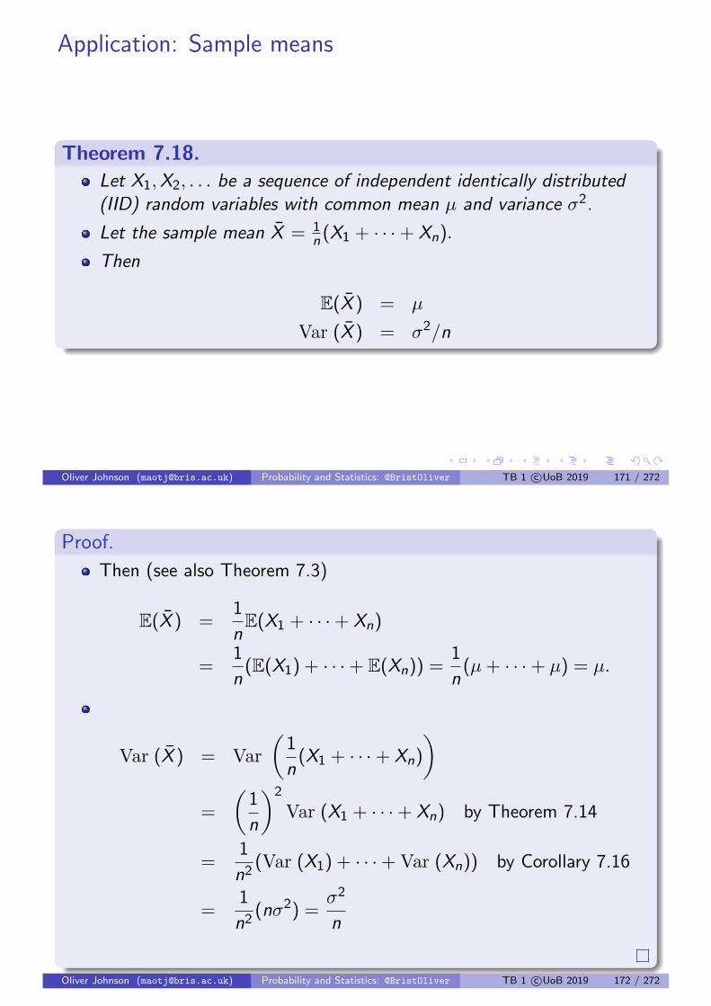
Application: Sample means
Theorem 7.18.
Let X1,X2, . . . be a sequence of independent identically distributed(IID) random variables with common mean µ and variance σ2.
Let the sample mean X = 1n (X1 + · · ·+ Xn).
Then
E(X ) = µ
Var (X ) = σ2/n
Oliver Johnson ([email protected]) Probability and Statistics: @BristOliver TB 1 c©UoB 2019 171 / 272
Proof.
Then (see also Theorem 7.3)
E(X ) =1
nE(X1 + · · ·+ Xn)
=1
n(E(X1) + · · ·+ E(Xn)) =
1
n(µ+ · · ·+ µ) = µ.
Var (X ) = Var
(1
n(X1 + · · ·+ Xn)
)=
(1
n
)2
Var (X1 + · · ·+ Xn) by Theorem 7.14
=1
n2(Var (X1) + · · ·+ Var (Xn)) by Corollary 7.16
=1
n2(nσ2) =
σ2
n
Oliver Johnson ([email protected]) Probability and Statistics: @BristOliver TB 1 c©UoB 2019 172 / 272

Example: coin toss (slight return)
Example 7.19.
For example, toss a fair coin repeatedly, and let
Xi =
1 if ith throw head0 if ith throw tail
Then X is the proportion of heads in the first n tosses.
E(X ) = E(Xi ) = 12 .
Var (Xi ) = 12 (1− 1
2 ) = 14 , so
Var (X ) =1
4n.
Oliver Johnson ([email protected]) Probability and Statistics: @BristOliver TB 1 c©UoB 2019 173 / 272
The weak law of large numbers
Let Y be any r.v. and let c > 0 be a positive constant.
Recall Chebyshev’s inequality (Theorem 5.21):
P(|Y − E(Y )| > c) ≤ Var (Y )
c2.
We know that E(X ) = µ and Var (X ) = σ2
n .
So taking Y = X in Chebyshev we deduce:
P(|X − µ| > c) ≤ σ2
nc2.
Theorem 7.20 (Weak law of large numbers).
Let X1,X2, . . . be a sequence of independent identically distributed (IID)random variables with common mean µ and variance σ2. Then for anyc > 0:
P(|X − µ| > c)→ 0 as n→∞.
Oliver Johnson ([email protected]) Probability and Statistics: @BristOliver TB 1 c©UoB 2019 174 / 272

Application to coin tossing
Example 7.21.
As in Example 7.19, let X be the proportion of heads in first n tosses.
Then µ = 12 and σ2 = 1
4 . Thus
P(∣∣∣∣X − 1
2
∣∣∣∣ > c
)≤ 1
4nc2.
So for example taking c = 0.01:
P(0.49 < X < 0.51) ≥ 1− 2500
n.
This tends to one as n→∞.
In fact the inequalities are very conservative here.
Axioms and definitions match our intuitive beliefs about probability.Closely related to central limit theorem (see later) and other laws oflarge numbers (see Probability 2).
Oliver Johnson ([email protected]) Probability and Statistics: @BristOliver TB 1 c©UoB 2019 175 / 272
Section 7.5: Examples
Example 7.22.
An urn contains two biased coins.
Coin 1 has a probability 13 of showing a head.
Coin 2 has a probability 23 of showing a head.
A coin is selected at random and the same coin is tossed twice.
Let X =
1 if 1st toss is H0 if 1st toss is T
and Y =
1 if 2nd toss is H0 if 2nd toss is T
Let W = X + Y be the total number of heads. Find Cov (X ,Y ),E(W ), Var (W ).
Oliver Johnson ([email protected]) Probability and Statistics: @BristOliver TB 1 c©UoB 2019 176 / 272

Urn example (cont.)
Example 7.22.
P(X = 1,Y = 1) = P(X = 1,Y = 1 | coin 1)P(coin 1)
+P(X = 1,Y = 1 | coin 2)P(coin 2)
=
(1
3
)2 1
2+
(2
3
)2 1
2=
5
18
Similarly for the other values
pX ,Y (x , y) y = 0 y = 1 pX (x)
x = 0 518
418
12
x = 1 418
518
12
pY (y) 12
12
X and Y are Bernoulli( 12 ) r.v.s, so E(X ) = E(Y ) = 1
2 andVar (X ) = Var (Y ) = 1
4 , and E(W ) = E(X ) + E(Y ) = 1.
Oliver Johnson ([email protected]) Probability and Statistics: @BristOliver TB 1 c©UoB 2019 177 / 272
Urn example (cont.)
Example 7.22.
E(XY ) = 0× 0× pX ,Y (0, 0) + 0× 1× pX ,Y (0, 1)
+1× 0× pX ,Y (1, 0) + 1× 1× pX ,Y (1, 1) =5
18.
Thus Cov (X ,Y ) = E(XY )− E(X )E(Y ) = 518 − ( 1
2 )2 = 136 .
Further, since Var (X ) = 14 , Var (Y ) = 1
4 , we know ρ(X ,Y ) = 19 .
Var (W ) = Var (X ) + 2Cov (X ,Y ) + Var (Y ) =1
4+
2
36+
1
4=
5
9.
Compare with Bin(2, 12 ) when variance = 1
2 .
Oliver Johnson ([email protected]) Probability and Statistics: @BristOliver TB 1 c©UoB 2019 178 / 272
Further example
Example 7.23.
A fair coin is tossed 10 times.
Let X be the number of heads in the first 5 tosses and let Y be thetotal number of heads.
We will find ρ(X ,Y ).
First note that since X and Y are both binomially distributed we have
Var (X ) =5
4
Var (Y ) =5
2.
Oliver Johnson ([email protected]) Probability and Statistics: @BristOliver TB 1 c©UoB 2019 179 / 272
Further example (cont.)
Example 7.23.
To find the covariance of X and Y it is convenient to set Z = Y −X .
Note that Z is the number of heads in the last 5 tosses.
Thus X and Z are independent. This implies that Cov (X ,Z ) = 0.Thus
Cov (X ,Y ) = Cov (X ,X + Z ) = Cov (X ,X ) + Cov (X ,Z )
= Var (X ) + 0 =5
4.
Thus
ρ(X ,Y ) =Cov (X ,Y )√Var (X )Var (Y )
=1√2.
Oliver Johnson ([email protected]) Probability and Statistics: @BristOliver TB 1 c©UoB 2019 180 / 272

Section 8: Continuous random variables I
Objectives: by the end of this section you should be able to
Understand continuous random variables.Interpret density and distribution functions.Know how to calculate means and variances of continuousrandom variables.Understand the basic properties of the exponential and gammadistributions.
[This material is also covered in Sections 5.1, 5.2, 5.3 and 5.5 of thecourse book]
Oliver Johnson ([email protected]) Probability and Statistics: @BristOliver TB 1 c©UoB 2019 181 / 272
Section 8.1: Motivation and definition
Remark 8.1.
So far we studied r.v.s that take a discrete (countable) set of values.
Many r.v.s take a continuum of values e.g. height, weight, time,temperature are real-valued.
Let X be the time till an atom decays (in seconds). ThenP(X = π) = 0.
But we expectP(π ≤ X ≤ π + δ) ≈ const× δ
for δ small.
In general P(X = x) = 0 for any particular x and we expect
P(x ≤ X ≤ x + δ) ≈ fX (x)δ
for δ small.
Think of fX (x) as an ‘intensity’ – won’t generally be 0.
Oliver Johnson ([email protected]) Probability and Statistics: @BristOliver TB 1 c©UoB 2019 182 / 272

Remark 8.1.
Consider an interval [a, b].
Divide it up into n segments of equal size
a = x0 < x1 < · · · < xn = b
with δ = xi − xi−1 = (b − a)/n for i = 1, . . . , n.
Then
P(a ≤ X < b) = P
(n⋃
i=1
xi−1 ≤ X < xi
)
=n∑
i=1
P(xi−1 ≤ X < xi ) ≈n∑
i=1
fX (xi−1)δ.
As n→∞,∑n
i=1 fX (xi−1)δ →∫ ba fX (x) dx .
So we expect P(a ≤ X < b) =∫ ba fX (x) dx .
Oliver Johnson ([email protected]) Probability and Statistics: @BristOliver TB 1 c©UoB 2019 183 / 272
Continuous random variables
Definition 8.2.
A random variable X has a continuous distribution if there exists afunction fX : R→ R such that
P(a ≤ X < b) =
∫ b
afX (x) dx for all a, b with a < b.
The function fX (x) is called the probability density function (pdf) for X .
Oliver Johnson ([email protected]) Probability and Statistics: @BristOliver TB 1 c©UoB 2019 184 / 272

Remark 8.3.
Suppose that X is a continuous r.v., then
P(X = x) = 0 for all x , so
P(a ≤ X < b) = P(a ≤ X ≤ b).
Special case:P(X ≤ b) = P(X < b) = lima→−∞ P(a ≤ X ≤ b) =
∫ b−∞ fX (x) dx .
Since P(−∞ < X <∞) = 1 we have∫ ∞−∞
fX (x) dx = 1.
fX (x) is not a probability. In particular we can have fX (x) > 1.
However fX (x) ≥ 0.
Oliver Johnson ([email protected]) Probability and Statistics: @BristOliver TB 1 c©UoB 2019 185 / 272
Section 8.2: Mean and variance
Definition 8.4.
Let X be a continuous r.v. with pdf fX (x). The mean or expectation of Xis
E(X ) =
∫ ∞−∞
xfX (x) dx .
Lemma 8.5.
Let X be a continuous r.v. with pdf fX (x) and Z = g(X ) for somefunction g . Then
E(Z ) = E(g(X )) =
∫ ∞−∞
g(x)fX (x) dx .
Note that x is a dummy variable.Note that in general we need to integrate over x from −∞ to ∞.However (see e.g. Example 8.7) we only need to consider the rangewhere fX (x) > 0.
Oliver Johnson ([email protected]) Probability and Statistics: @BristOliver TB 1 c©UoB 2019 186 / 272
Variance
Definition 8.6.
The variance of X is
Var (X ) = E((X − µ)2),
where µ is shorthand for E(X ). As before we can show that
Var (X ) = E(X 2)− (E(X ))2.
Oliver Johnson ([email protected]) Probability and Statistics: @BristOliver TB 1 c©UoB 2019 187 / 272
Uniform distribution
Example 8.7.
Suppose the density fX (x) = 1 for 0 ≤ x ≤ 1 and 0 otherwise.
May be best to represent this with an indicator function I.Can write fX (x) = I(0 ≤ x ≤ 1).
We know that this is a valid density function since∫ ∞−∞
fX (x)dx =
∫ ∞−∞
I(0 ≤ x ≤ 1)dx =
∫ 1
01dx = 1.
We call this the Uniform distribution on [0, 1].
Generalize: given a < b, uniform distribution on [a, b] has density
fY (y) =1
b − aI(a ≤ y ≤ b).
Write Y ∼ U(a, b).
Oliver Johnson ([email protected]) Probability and Statistics: @BristOliver TB 1 c©UoB 2019 188 / 272

Uniform distribution
Example 8.7.
If X is uniform on [0, 1]:
E(X ) =
∫ ∞−∞
xfX (x)dx =
∫ 1
0xdx =
[x2
2
]1
0
=1
2,
E(X 2) =
∫ ∞−∞
x2fX (x)dx =
∫ 1
0x2dx =
[x3
3
]1
0
=1
3,
so that Var (X ) = E(X 2)− (E(X ))2 = 13 −
122 = 1
12 .
Similarly if Y is uniform on [a, b]:
E(Y ) =
∫ ∞−∞
xfY (x)dx =
∫ b
a
x
b − adx
=1
b − a
[x2
2
]ba
=b2 − a2
2(b − a)=
a + b
2.
Oliver Johnson ([email protected]) Probability and Statistics: @BristOliver TB 1 c©UoB 2019 189 / 272
Section 8.3: The distribution function
Definition 8.8.
For any r.v. X , the (cumulative) distribution function of X is defined asthe function FX : R→ [0, 1] given by
FX (x) = P(X ≤ x) for x ∈ R.
Lemma 8.9.
In fact, these hold for any r.v. whether discrete, continuous or other:
P(a < X ≤ b) = FX (b)− FX (a)
FX (x) is an increasing function of x
FX (x)→ 0 as x → −∞FX (x)→ 1 as x →∞
Oliver Johnson ([email protected]) Probability and Statistics: @BristOliver TB 1 c©UoB 2019 190 / 272

Distribution and density function
Lemma 8.10.
Let X have a continuous distribution. Then (y is a dummy variable)
FX (x) = P(X ≤ x) =
∫ x
−∞fX (y) dy for all x ∈ R.
P(X ≤ x) is the area under the density function to the left of x .Hence we have that F ′X (x) = fX (x).Note that when X is continuous, P(X = x) = 0 for all x so
FX (x) = P(X ≤ x) = P(X < x).
Example 8.11.
In the uniform random variable setting of Example 8.7, the
FX (x) =
0 for x ≤ 0,x for 0 ≤ x ≤ 1,1 for 1 ≤ x .
Oliver Johnson ([email protected]) Probability and Statistics: @BristOliver TB 1 c©UoB 2019 191 / 272
Example
Example 8.12.
Suppose X has a continuous distribution with density function
fX (x) =
0 x ≤ 12x3 x > 1
Find FX .
Let x ≤ 1. Then
FX (x) =
∫ x
−∞fX (y) dy =
∫ x
−∞0 dy = 0.
Oliver Johnson ([email protected]) Probability and Statistics: @BristOliver TB 1 c©UoB 2019 192 / 272
Example (cont.)
Example 8.12.
Let x > 1. Then
FX (x) =
∫ x
−∞fX (y) dy =
∫ 1
−∞0 dy +
∫ x
1
2
y3dy = 0 +
[−1
y2
]x1
=−1
x2− −1
1= 1− 1
x2.
So FX (x) =
0 x ≤ 1
1− 1x2 x > 1
Note: the integrals have limits. Don’t write FX (x) =∫fX (y) dy without
limits then determine C . It is both confusing and sloppy!
Oliver Johnson ([email protected]) Probability and Statistics: @BristOliver TB 1 c©UoB 2019 193 / 272
Continuous convolution
Recall the discrete convolution formula (Proposition 6.17)
pX+Y (k) =∞∑
i=−∞pX (k − i) · pY (i), for all k ∈ Z.
In a very similar way we state without proof the continuous convolutionformula for densities:
Proposition 8.13.
Suppose X and Y are independent continuous random variables withrespective densities fX and fY . Then their sum is a continuous randomvariable with density
fX+Y (z) =
∫ ∞−∞
fX (z − y) · fY (y) dy , for all z ∈ R.
Oliver Johnson ([email protected]) Probability and Statistics: @BristOliver TB 1 c©UoB 2019 194 / 272

Section 8.4: Examples of continuous random variables
Let T be the time to wait for an event e.g. a bus to arrive, or aradioactive decay to occur.
Suppose that if the event has not happened by t then the probabilitythat it happens in (t, t + δ) is λδ + o(δ) (i.e. it doesn’t depend on t).
Then (for t > 0) FT (t) = P(T ≤ t) = 1− e−λt and fT (t) = λe−λt .See why in Probability 2.
Definition 8.14.
A r.v. T has an exponential distribution with rate parameter λ if ithas a continuous distribution with density
fT (t) =
0 t ≤ 0
λe−λt t > 0
Notation T ∼ Exp(λ).
Oliver Johnson ([email protected]) Probability and Statistics: @BristOliver TB 1 c©UoB 2019 195 / 272
Exponential distribution properties
Remark 8.15.
P(T > t) = 1− P(T ≤ t) = e−λt
E(T ) =
∫ ∞−∞
tfT (t) dt =
∫ ∞0
tλe−λt dt
=[−te−λt
]∞0
+
∫ ∞0
e−λt dt
= 0 +1
λ
Var (T ) =1
λ2(Exercise).
Oliver Johnson ([email protected]) Probability and Statistics: @BristOliver TB 1 c©UoB 2019 196 / 272
Exponential distribution properties (cont.)
Remark 8.15.
Exponential is continuous analogue of the geometric distribution.
In particular it has the lack of memory property (cf Lemma 4.19):
P(T > t + s |T > s) =P(T > t + s and T > s)
P(T > s)
=P(T > t + s)
P(T > s)
=e−λ(t+s)
e−λs
= e−λt
= P(T > t).
Oliver Johnson ([email protected]) Probability and Statistics: @BristOliver TB 1 c©UoB 2019 197 / 272
Section 8.5: Gamma distributions
Definition 8.16.
For α > 0 define the gamma function
Γ(α) =
∫ ∞0
xα−1e−x dx .
We will see that this is a generalisation of the (shifted) factorial function.
Oliver Johnson ([email protected]) Probability and Statistics: @BristOliver TB 1 c©UoB 2019 198 / 272
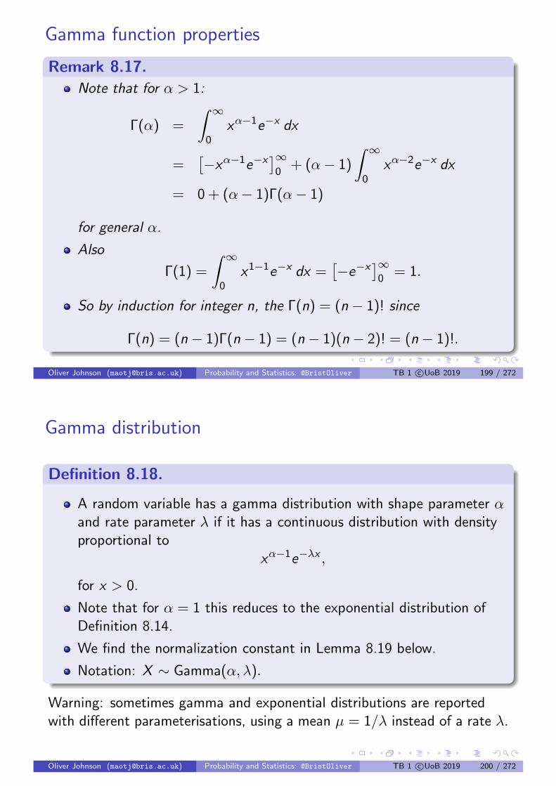
Gamma function properties
Remark 8.17.
Note that for α > 1:
Γ(α) =
∫ ∞0
xα−1e−x dx
=[−xα−1e−x
]∞0
+ (α− 1)
∫ ∞0
xα−2e−x dx
= 0 + (α− 1)Γ(α− 1)
for general α.
Also
Γ(1) =
∫ ∞0
x1−1e−x dx =[−e−x
]∞0
= 1.
So by induction for integer n, the Γ(n) = (n − 1)! since
Γ(n) = (n − 1)Γ(n − 1) = (n − 1)(n − 2)! = (n − 1)!.
Oliver Johnson ([email protected]) Probability and Statistics: @BristOliver TB 1 c©UoB 2019 199 / 272
Gamma distribution
Definition 8.18.
A random variable has a gamma distribution with shape parameter αand rate parameter λ if it has a continuous distribution with densityproportional to
xα−1e−λx ,
for x > 0.
Note that for α = 1 this reduces to the exponential distribution ofDefinition 8.14.
We find the normalization constant in Lemma 8.19 below.
Notation: X ∼ Gamma(α, λ).
Warning: sometimes gamma and exponential distributions are reportedwith different parameterisations, using a mean µ = 1/λ instead of a rate λ.
Oliver Johnson ([email protected]) Probability and Statistics: @BristOliver TB 1 c©UoB 2019 200 / 272

Lemma 8.19.
Let X ∼ Gamma(α, λ). Then
fX (x) =
λα
Γ(α)xα−1e−λx x > 0,
0 x ≤ 0.
Proof.
For x > 0, fX (x) = Cxα−1e−λx for some constant C . We know
1 =
∫ ∞−∞
fX (x) dx
=
∫ ∞0
Cxα−1e−λx dx
= C
∫ ∞0
(yλ
)α−1e−y
dy
λsetting y = λx
=C
λα
∫ ∞0
yα−1e−y dy =C
λαΓ(α).
Oliver Johnson ([email protected]) Probability and Statistics: @BristOliver TB 1 c©UoB 2019 201 / 272
Gamma distribution properties
Remark 8.20.
If α = 1 then fX (x) =
0 x ≤ 0
λe−λx x > 0.I.e. if X ∼ Gamma(1, λ) then X ∼ Exp(λ).
In Proposition 8.21 (see also Lemma 11.13) we will see that (forinteger α) a Gamma(α, λ) r.v. has the same distribution as the sumof α independent Exp(λ) r.v.s
Proposition 8.21.
If X ∼ Gamma(α, λ) and Y ∼ Gamma(β, λ) are independent, then theirsum X + Y ∼ Gamma(α + β, λ).
Oliver Johnson ([email protected]) Probability and Statistics: @BristOliver TB 1 c©UoB 2019 202 / 272

Proof of Proposition 8.21 (integer α, β)
Proof.
By Proposition 8.13 we know that the density of X + Y is the convolution
fX+Y (z) =
∫ ∞−∞
fX (z − y) · fY (y)dy
=
∫ z
0fX (z − y) · fY (y)dy
=
∫ z
0
λα
Γ(α)(z − y)α−1e−λ(z−y) · λ
β
Γ(β)yβ−1e−λydy
=λα+β
Γ(α)Γ(β)e−λz
∫ z
0(z − y)α−1yβ−1dy
=:λα+β
Γ(α)Γ(β)e−λz Iα,β.
Oliver Johnson ([email protected]) Probability and Statistics: @BristOliver TB 1 c©UoB 2019 203 / 272
Proof of Proposition 8.21 (integer α, β, cont.)
Proof.
This integral, known as a beta integral, equalsIα,β = zα+β−1Γ(α)Γ(β)/Γ(α + β), as required.
This follows in integer case by induction, since we can write it aszα+β−1(α− 1)!(β − 1)!/(α + β − 1)!
Value found using integration by parts (since function vanishes ateither end of support):
Iα,β =
∫ z
0(z − y)α−1yβ−1dy
=
∫ z
0(α− 1)(z − y)α−2 y
β
βdy =
α− 1
βIα−1,β+1.
We use the fact that I1,β =∫ z
0 yβ−1 = zβ
β .
Oliver Johnson ([email protected]) Probability and Statistics: @BristOliver TB 1 c©UoB 2019 204 / 272

Gamma distribution properties (cont.)
Remark 8.21.
E(X ) =
∫ ∞0
xλα
Γ(α)xα−1e−λx dx
=λα
Γ(α)
∫ ∞0
xαe−λx dx
=λα
Γ(α)
Γ(α + 1)
λα+1
∫ ∞0
λα+1
Γ(α + 1)xαe−λx dx
=λα
Γ(α)
Γ(α + 1)
λα+1
∫ ∞0
fY (x) dx where Y ∼ Gamma(α + 1, λ)
=αΓ(α)
λΓ(α)× 1 =
α
λ
Similarly Var (X ) =α
λ2.
Oliver Johnson ([email protected]) Probability and Statistics: @BristOliver TB 1 c©UoB 2019 205 / 272
Section 9: Continuous random variables II
Objectives: by the end of this section you should be able to
Understand transformations of continuous random variables.Describe normal random variables and use tables to calculateprobabilities.Consider jointly distributed continuous random variables.
[This material is also covered in Sections 5.4, 5.7 and 6.1 of the coursebook]
Oliver Johnson ([email protected]) Probability and Statistics: @BristOliver TB 1 c©UoB 2019 206 / 272
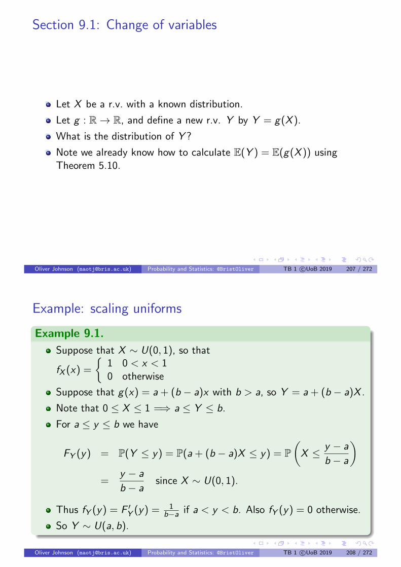
Section 9.1: Change of variables
Let X be a r.v. with a known distribution.
Let g : R→ R, and define a new r.v. Y by Y = g(X ).
What is the distribution of Y ?
Note we already know how to calculate E(Y ) = E(g(X )) usingTheorem 5.10.
Oliver Johnson ([email protected]) Probability and Statistics: @BristOliver TB 1 c©UoB 2019 207 / 272
Example: scaling uniforms
Example 9.1.
Suppose that X ∼ U(0, 1), so that
fX (x) =
1 0 < x < 10 otherwise
Suppose that g(x) = a + (b − a)x with b > a, so Y = a + (b − a)X .
Note that 0 ≤ X ≤ 1 =⇒ a ≤ Y ≤ b.
For a ≤ y ≤ b we have
FY (y) = P(Y ≤ y) = P(a + (b − a)X ≤ y) = P(X ≤ y − a
b − a
)=
y − a
b − asince X ∼ U(0, 1).
Thus fY (y) = F ′Y (y) = 1b−a if a < y < b. Also fY (y) = 0 otherwise.
So Y ∼ U(a, b).
Oliver Johnson ([email protected]) Probability and Statistics: @BristOliver TB 1 c©UoB 2019 208 / 272

General case
Lemma 9.2.
Let X be a r.v. taking values in I ⊆ R. Let Y = g(X ) where g : I → J isstrictly monotonic and differentiable on I with inverse function h = g−1.Then
fY (y) =
fX (h(y))|h′(y)| y ∈ J
0 y /∈ J.
Proof.
X takes values in I , and g : I → J, so Y takes values in J.
Therefore fY (y) = 0 for y /∈ J.
Case 1 Assume first that g is strictly increasing. For y ∈ J
FY (y) = P(Y ≤ y) = P(g(X ) ≤ y) = P(X ≤ h(y)) = FX (h(y)).
So fY (y) = F ′Y (y) = F ′X (h(y))h′(y) = fX (h(y))h′(y) by chain rule.
Oliver Johnson ([email protected]) Probability and Statistics: @BristOliver TB 1 c©UoB 2019 209 / 272
Proof of Lemma 9.2 (cont.)
Proof.
Case 2 Now assume g is strictly decreasing. For y ∈ J
FY (y) = P(g(X ) ≤ y) = P(X ≥ h(y))
= 1− P(X < h(y)) = 1− FX (h(y)).
So fY (y) = −fX (h(y))h′(y).
But g (and therefore h) are strictly decreasing, so h′(y) < 0, and−h′(y) = |h′(y)|.
Oliver Johnson ([email protected]) Probability and Statistics: @BristOliver TB 1 c©UoB 2019 210 / 272

Simulation of random variables
In general computers can give you U(0, 1) random numbers andnothing else.
You need to transform these U(0, 1) to give you something useful.
Example 9.3.
Let X ∼ U(0, 1) and let Y = 1λ log
(1
1−X
).
What is the distribution of Y ?
Define g : (0, 1)→ (0,∞) by g(x) = 1λ log
(1
1−x
).
To find the inverse of the function g set
y =1
λlog
(1
1− x
)=⇒ −λy = log(1− x)
=⇒ x = 1− e−λy
Oliver Johnson ([email protected]) Probability and Statistics: @BristOliver TB 1 c©UoB 2019 211 / 272
Simulation of random variables (cont.)
Example 9.3.
That is, the inverse function h is given by h(y) = 1− e−λy .
The image of the function g is J = (0,∞), so fY (y) = 0 for y ≤ 0.
Let y > 0. Then fY (y) = fX (h(y))|h′(y)| = 1× λe−λy .
So Y ∼ Exp(λ).
To generate Exp(λ) random variables, you take the U(0, 1) r.v.s givenby the computer and apply g .
Oliver Johnson ([email protected]) Probability and Statistics: @BristOliver TB 1 c©UoB 2019 212 / 272
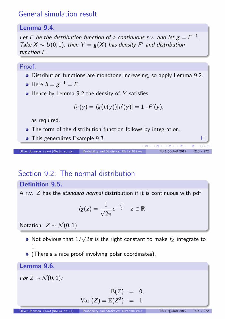
General simulation result
Lemma 9.4.
Let F be the distribution function of a continuous r.v. and let g = F−1.Take X ∼ U(0, 1), then Y = g(X ) has density F ′ and distributionfunction F .
Proof.
Distribution functions are monotone increasing, so apply Lemma 9.2.
Here h = g−1 = F .
Hence by Lemma 9.2 the density of Y satisfies
fY (y) = fX (h(y))|h′(y)| = 1 · F ′(y),
as required.
The form of the distribution function follows by integration.
This generalizes Example 9.3.
Oliver Johnson ([email protected]) Probability and Statistics: @BristOliver TB 1 c©UoB 2019 213 / 272
Section 9.2: The normal distribution
Definition 9.5.
A r.v. Z has the standard normal distribution if it is continuous with pdf
fZ (z) =1√2π
e−z2
2 z ∈ R.
Notation: Z ∼ N (0, 1).
Not obvious that 1/√
2π is the right constant to make fZ integrate to1.(There’s a nice proof involving polar coordinates).
Lemma 9.6.
For Z ∼ N (0, 1):
E(Z ) = 0,
Var (Z ) = E(Z 2) = 1.
Oliver Johnson ([email protected]) Probability and Statistics: @BristOliver TB 1 c©UoB 2019 214 / 272

Proof of Lemma 9.6
Proof.
fZ (z) is symmetric about 0. So
E(Z ) =
∫ ∞−∞
zfZ (z) dz = 0.
Alternatively, notice that zfZ (z) = − ddz fZ (z) so that
E(Z ) =
∫ ∞−∞
zfZ (z) dz = −∫ ∞−∞
(d
dzfZ (z)
)dz = [fZ (z)]∞−∞ = 0.
Similarly, integration by parts gives
E(Z 2) =1√2π
∫ ∞−∞
z(ze−z2
2 ) dz =1√2π
∫ ∞−∞
e−z2
2 dz = 1.
So Var (Z ) = E(Z 2)− (E(Z ))2 = 1.
Oliver Johnson ([email protected]) Probability and Statistics: @BristOliver TB 1 c©UoB 2019 215 / 272
General normal distribution properties
Remark 9.7.
Often fZ (z) is denoted φ(z) and FZ (z) is denoted Φ(z).
Not possible to write down a formula for Φ(z) using ‘standardfunctions’.
Instead values of Φ(z) are in tables, or can be calculated bycomputer. See second half of course.
Definition 9.8.
A r.v. X has a normal distribution with mean µ and variance σ2 if it iscontinuous with pdf
fX (x) =1√
2πσ2exp
−(x − µ)2
2σ2
.
Notation: X ∼ N (µ, σ2).
Oliver Johnson ([email protected]) Probability and Statistics: @BristOliver TB 1 c©UoB 2019 216 / 272

General normal distribution properties (cont.)
Lemma 9.9.
Let X ∼ N (µ, σ2) and define Z = X−µσ . Then Z ∼ N (0, 1).
Proof.
Z = g(X ) where g(x) = x−µσ .
If z = g(x) = x−µσ then x = µ+ σz so h(z) = µ+ σz = g−1(z).
Therefore by Lemma 9.2
fZ (z) = fX (h(z))|h′(z)|
=1√
2πσ2exp
−(h(z)− µ)2
2σ2
× σ
=1√2π
exp
−(µ+ σz − µ)2
2σ2
=
1√2π
exp
−z2
2
.
Oliver Johnson ([email protected]) Probability and Statistics: @BristOliver TB 1 c©UoB 2019 217 / 272
General normal distribution properties (cont.)
Corollary 9.10.
Let X ∼ N (µ, σ2). Then E(X ) = µ and Var (X ) = σ2.
Proof.
We know that Z = X−µσ ∼ N (0, 1), so E(Z ) = 0 and Var (Z ) = 1.
So 0 = E(Z ) = E(X−µσ
)= E(X )−µ
σ and E(X ) = µ.
Also 1 = Var (Z ) = Var(X−µσ
)= Var (X )
σ2 .
Many quantities have an approximate normal distribution.
For example heights in a population, measurement errors.
There are good theoretical reasons for this (see Theorem 11.21).
The normal distribution is very important in statistics.
Oliver Johnson ([email protected]) Probability and Statistics: @BristOliver TB 1 c©UoB 2019 218 / 272

Normal convergence
Theorem 9.11 (DeMoivre-Laplace).
Fix p, and let Xn ∼ Bin(n, p). Then for every fixed a < b,
limn→∞
P
(a <
Xn − np√np(1− p)
≤ b
)= Φ(b)− Φ(a).
That is, take X ∼ Bin(n, p) with large n and fixed p.
Then Xn−np√np(1−p)
is approximately N(0, 1) distributed.
This is a special case of the Central Limit Theorem, Theorem 11.21.
Oliver Johnson ([email protected]) Probability and Statistics: @BristOliver TB 1 c©UoB 2019 219 / 272
Normal distribution tables
Φ(z)z 0.00 0.01 0.02 0.03 0.04 0.05 0.06 0.07 0.08 0.09
0.0 0.5000 0.5040 0.5080 0.5120 0.5160 0.5199 0.5239 0.5279 0.5319 0.53590.1 0.5398 0.5438 0.5478 0.5517 0.5557 0.5596 0.5636 0.5675 0.5714 0.57530.2 0.5793 0.5832 0.5871 0.5910 0.5948 0.5987 0.6026 0.6064 0.6103 0.61410.3 0.6179 0.6217 0.6255 0.6293 0.6331 0.6368 0.6406 0.6443 0.6480 0.65170.4 0.6554 0.6591 0.6628 0.6664 0.6700 0.6736 0.6772 0.6808 0.6844 0.68790.5 0.6915 0.6950 0.6985 0.7019 0.7054 0.7088 0.7123 0.7157 0.7190 0.72240.6 0.7257 0.7291 0.7324 0.7357 0.7389 0.7422 0.7454 0.7486 0.7517 0.75490.7 0.7580 0.7611 0.7642 0.7673 0.7704 0.7734 0.7764 0.7794 0.7823 0.78520.8 0.7881 0.7910 0.7939 0.7967 0.7995 0.8023 0.8051 0.8078 0.8106 0.81330.9 0.8159 0.8186 0.8212 0.8238 0.8264 0.8289 0.8315 0.8340 0.8365 0.83891.0 0.8413 0.8438 0.8461 0.8485 0.8508 0.8531 0.8554 0.8577 0.8599 0.86211.1 0.8643 0.8665 0.8686 0.8708 0.8729 0.8749 0.8770 0.8790 0.8810 0.88301.2 0.8849 0.8869 0.8888 0.8907 0.8925 0.8944 0.8962 0.8980 0.8997 0.90151.3 0.9032 0.9049 0.9066 0.9082 0.9099 0.9115 0.9131 0.9147 0.9162 0.91771.4 0.9192 0.9207 0.9222 0.9236 0.9251 0.9265 0.9279 0.9292 0.9306 0.93191.5 0.9332 0.9345 0.9357 0.9370 0.9382 0.9394 0.9406 0.9418 0.9429 0.94411.6 0.9452 0.9463 0.9474 0.9484 0.9495 0.9505 0.9515 0.9525 0.9535 0.95451.7 0.9554 0.9564 0.9573 0.9582 0.9591 0.9599 0.9608 0.9616 0.9625 0.96331.8 0.9641 0.9649 0.9656 0.9664 0.9671 0.9678 0.9686 0.9693 0.9699 0.97061.9 0.9713 0.9719 0.9726 0.9732 0.9738 0.9744 0.9750 0.9756 0.9761 0.97672.0 0.9772 0.9778 0.9783 0.9788 0.9793 0.9798 0.9803 0.9808 0.9812 0.98172.1 0.9821 0.9826 0.9830 0.9834 0.9838 0.9842 0.9846 0.9850 0.9854 0.98572.2 0.9861 0.9864 0.9868 0.9871 0.9875 0.9878 0.9881 0.9884 0.9887 0.98902.3 0.9893 0.9896 0.9898 0.9901 0.9904 0.9906 0.9909 0.9911 0.9913 0.99162.4 0.9918 0.9920 0.9922 0.9925 0.9927 0.9929 0.9931 0.9932 0.9934 0.9936
Oliver Johnson ([email protected]) Probability and Statistics: @BristOliver TB 1 c©UoB 2019 220 / 272

Application
Example 9.12.
The height of a randomly selected male student at Bristol has anormal distribution with mean 1.75m and standard deviation 0.05m.
A student is chosen at random. What is the probability his height isgreater than 1.86m?
Let X be the height of the student, so X ∼ N (1.75, (0.05)2).
Let Z = X−1.750.05 so that Z ∼ N (0, 1).
P(X > 1.86) = P(X − 1.75
0.05>
1.86− 1.75
0.05
)= P(Z > 2.2) = 1− P(Z ≤ 2.2) = 1− Φ(2.2)
Can find Φ(2.2) from tabulated values, or (when you’ve done Statspart of course) using a computer language called R.
The value is Φ(2.2) = 0.9861. So P(X > 1.86) = 0.0139.
Oliver Johnson ([email protected]) Probability and Statistics: @BristOliver TB 1 c©UoB 2019 221 / 272
Fact, proved in Section 11.4
Lemma 9.13.
If X ∼ N (µ, σ2) and Y ∼ N (ν, τ2) are independent then
X + Y ∼ N (µ+ ν, σ2 + τ2).
Very few random variables have this property that you can add themand still get a distribution in the same family.
Compare with the addition of Poissons in Theorem 6.18.
See Lemma 11.18 for full proof.
Oliver Johnson ([email protected]) Probability and Statistics: @BristOliver TB 1 c©UoB 2019 222 / 272

Section 9.3: Jointly distributed continuous r.v.s
Definition 9.14.
Let X and Y be continuous r.v.s. They are jointly distributed withdensity function
fX ,Y (x , y)
if for any region A ⊂ R2
P((X ,Y ) ∈ A) =
∫AfX ,Y (x , y) dxdy .
Marginal density for X is fX (x) =∫∞−∞ fX ,Y (x , y) dy .
Conditional density for X given Y = y is fX |Y (x | y) =fX ,Y (x ,y)fY (y) .
Similarly for Y .
X and Y are independent iff fX ,Y (x , y) = fX (x)fY (y) for all x , y ∈ R.
Oliver Johnson ([email protected]) Probability and Statistics: @BristOliver TB 1 c©UoB 2019 223 / 272
Time to wait for a lift while hitchhiking
Example 9.15.
You choose a site to hitchhike at random.
Let X be the site type and assume X ∼ Exp(1).
If the site type is x it takes an Exp(x) amount of time to get a lift (solarge x is good).
We have been given
fX (x) = e−x x > 0
fT |X (t|x) = xe−xt x , t > 0
Thus fX ,T (x , t) = fT |X (t|x)fX (x) = xe−(t+1)x for x , t > 0.
HencefT (t) =
∫∞−∞ fX ,T (x , t) dx =
∫∞0 xe−(t+1)x dx = Γ(2)
(t+1)2 = 1(t+1)2 .
Finally, P(T > t) =∫∞t fT (τ) dτ =
∫∞t
1(τ+1)2 dτ =
[−1τ+1
]∞t
= 1t+1 .
Oliver Johnson ([email protected]) Probability and Statistics: @BristOliver TB 1 c©UoB 2019 224 / 272
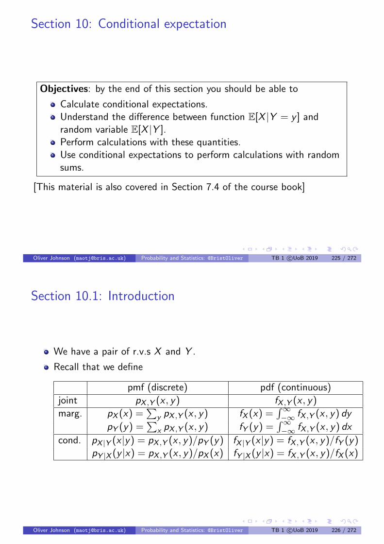
Section 10: Conditional expectation
Objectives: by the end of this section you should be able to
Calculate conditional expectations.Understand the difference between function E[X |Y = y ] andrandom variable E[X |Y ].Perform calculations with these quantities.Use conditional expectations to perform calculations with randomsums.
[This material is also covered in Section 7.4 of the course book]
Oliver Johnson ([email protected]) Probability and Statistics: @BristOliver TB 1 c©UoB 2019 225 / 272
Section 10.1: Introduction
We have a pair of r.v.s X and Y .
Recall that we define
pmf (discrete) pdf (continuous)
joint pX ,Y (x , y) fX ,Y (x , y)
marg. pX (x) =∑
y pX ,Y (x , y) fX (x) =∫∞−∞ fX ,Y (x , y) dy
pY (y) =∑
x pX ,Y (x , y) fY (y) =∫∞−∞ fX ,Y (x , y) dx
cond. pX |Y (x |y) = pX ,Y (x , y)/pY (y) fX |Y (x |y) = fX ,Y (x , y)/fY (y)pY |X (y |x) = pX ,Y (x , y)/pX (x) fY |X (y |x) = fX ,Y (x , y)/fX (x)
Oliver Johnson ([email protected]) Probability and Statistics: @BristOliver TB 1 c©UoB 2019 226 / 272

Conditional expectation definition
Definition 10.1.
Define E(X |Y = y) to be the expected value of X using the conditionaldistribution of X given that Y = y :
E(X |Y = y) =
∑x xpX |Y (x |y) X discrete∫∞
−∞ xfX |Y (x |y) dx X continuous
Oliver Johnson ([email protected]) Probability and Statistics: @BristOliver TB 1 c©UoB 2019 227 / 272
Example
Example 10.2.
X , Y discrete
pX ,Y (x , y) y = 0 1 2 3 pX (x)
x = 0 14 0 0 0 1
41 1
818 0 0 1
42 1
162
161
16 0 14
3 132
332
332
132
14
pY (y) 1532
1132
532
132
For E(X |Y = 0): pX |Y (x | 0) =pX ,Y (x ,0)pY (0) = 32
15pX ,Y (x , 0) so
x 0 1 2 3
pX |Y (x | 0) 815
415
215
115
So E(X |Y = 0) = 0× 815 + 1× 4
15 + 2× 215 + 3× 1
15 = 1115 .
Oliver Johnson ([email protected]) Probability and Statistics: @BristOliver TB 1 c©UoB 2019 228 / 272

Example (cont.)
Example 10.2.
Similarly
E(X |Y = 1) = 0× 0 + 1× 411 + 2× 4
11 + 3× 311 = 21
11E(X |Y = 2) = 0× 0 + 1× 0 + 2× 2
5 + 3× 35 = 13
5E(X |Y = 3) = 0× 0 + 1× 0 + 2× 0 + 3× 1 = 3
Remark 10.3.
It is vital to understand that:
E(X ) is a number
E(X |Y = y) is a function – specifically a function of y (call it A(y)).
We also define random variable E(X |Y ) = A(Y ) (pick value of Yrandomly, according to pY ).
Good to spend time thinking which type of object is which.
Oliver Johnson ([email protected]) Probability and Statistics: @BristOliver TB 1 c©UoB 2019 229 / 272
Section 10.2: Expectation of a conditional expectation
Theorem 10.4 (Tower Law aka Law of Total Expectation).
For any random variables X and Y , the E[X |Y ] is a random variable, with
E(X ) = E (E[X |Y ])
Remark 10.5.
For Y discrete
E (E[X |Y ]) =∑y
E(X |Y = y)P(Y = y).
For Y continuous
E (E[X |Y ]) =
∫ ∞−∞
E(X |Y = y)fY (y) dy .
Oliver Johnson ([email protected]) Probability and Statistics: @BristOliver TB 1 c©UoB 2019 230 / 272
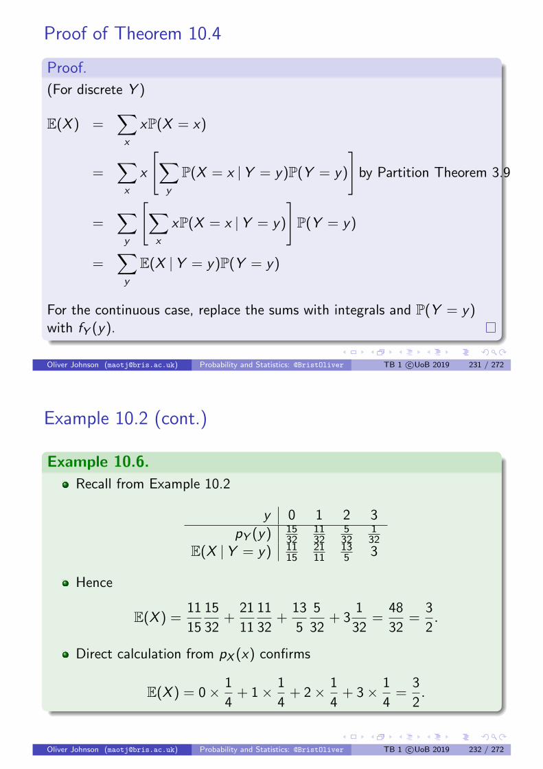
Proof of Theorem 10.4
Proof.
(For discrete Y )
E(X ) =∑x
xP(X = x)
=∑x
x
[∑y
P(X = x |Y = y)P(Y = y)
]by Partition Theorem 3.9
=∑y
[∑x
xP(X = x |Y = y)
]P(Y = y)
=∑y
E(X |Y = y)P(Y = y)
For the continuous case, replace the sums with integrals and P(Y = y)with fY (y).
Oliver Johnson ([email protected]) Probability and Statistics: @BristOliver TB 1 c©UoB 2019 231 / 272
Example 10.2 (cont.)
Example 10.6.
Recall from Example 10.2
y 0 1 2 3
pY (y) 1532
1132
532
132
E(X |Y = y) 1115
2111
135 3
Hence
E(X ) =11
15
15
32+
21
11
11
32+
13
5
5
32+ 3
1
32=
48
32=
3
2.
Direct calculation from pX (x) confirms
E(X ) = 0× 1
4+ 1× 1
4+ 2× 1
4+ 3× 1
4=
3
2.
Oliver Johnson ([email protected]) Probability and Statistics: @BristOliver TB 1 c©UoB 2019 232 / 272

Tower law example
Example 10.7.
A disoriented miner finds himself in a room of the mine with threedoors:
I The first door brings him to safety after a 3 hours long hike.I The second door takes him back to the same room after 5 hours of
climbing.I The third door takes him again back to the same room after 7 hours of
exhausting climbing.
The disoriented miner chooses one of the three doors with equalchance independently each time he is in that room.
What is the expected time after which the miner is safe?
Oliver Johnson ([email protected]) Probability and Statistics: @BristOliver TB 1 c©UoB 2019 233 / 272
Tower law example (cont.)
Example 10.7.
Let X be the time to reach safety, and Y the initial choice of a door(= 1, 2, 3). Then using Theorem 10.4
EX = E (E(X |Y ))
= E(X |Y = 1) · P(Y = 1) + E(X |Y = 2) · P(Y = 2)
+ E(X |Y = 3) · P(Y = 3)
= 3 · 1
3+ (EX + 5) · 1
3+ (EX + 7) · 1
3,
which we rearrange as
3EX = 15 + 2EX ; EX = 15.
Oliver Johnson ([email protected]) Probability and Statistics: @BristOliver TB 1 c©UoB 2019 234 / 272

Example
Example 10.8.
Nuts in a wood have an intrinsic hardness H, a non-negative integerrandom variable.
The hardness H of a randomly selected nut has a Poi(1) distribution.
If a nut has hardness H = h a squirrel takes a geometric 1h+1 number
of attempts to crack the nut.
What is the expected number of attempts taken to crack a randomlyselected nut?
Let X be the number of attempts. We want E(X ).
Given H = h, X ∼ Geom( 1h+1 ), so E(X |H = h) = 1
1h+1
= h + 1.
ThereforeE(X ) = E(E(X |H)) = E(A(H)) = E(H +1) = E(H)+1 = 1+1 = 2.
Oliver Johnson ([email protected]) Probability and Statistics: @BristOliver TB 1 c©UoB 2019 235 / 272
Important notation
Remark 10.9.
Remember from Remark 10.3 that E(X |Y = y) is a function of y .
Set A(y) = E(X |Y = y).
Then the Tower Law (Theorem 10.4) givesE(X ) =
∑y E(X |Y = y)P(Y = y) =
∑y A(y)P(Y = y) =
E(A(Y )).
Remember A(Y ) is a random variable that we often write as E(X |Y ).
Example 10.10.
In the nut example, Example 10.8 A(h) = E(X |H = h) = h + 1.
Hence A(H) = H + 1 i.e. E(X |H) = H + 1 [NB FUNCTION OF H].
ThereforeE(X ) = E(E(X |H)) = E(A(H)) = E(H + 1) = E(H) + 1 = 2.
Oliver Johnson ([email protected]) Probability and Statistics: @BristOliver TB 1 c©UoB 2019 236 / 272

Section 10.3: Conditional variance
Definition 10.11.
The conditional variance of X , given Y is
Var (X |Y ) = E[(X − E(X |Y ))2 |Y
]= E(X 2 |Y )−
[E(X |Y )
]2.
No surprise here, just use conditionals everywhere in the definition ofvariance.
Notice that Var (X |Y ) is again a function of Y (a random variable).
If we write A(Y ) for[E(X |Y )
]then we can rewrite Definition 10.11
asVar (X |Y ) = E(X 2 |Y )− A(Y )2. (10.1)
Oliver Johnson ([email protected]) Probability and Statistics: @BristOliver TB 1 c©UoB 2019 237 / 272
Law of Total Variance
Proposition 10.12.
The Law of Total Variance holds:
Var X = E (Var (X |Y )) + Var (E(X |Y )) .
In words: the variance is the expectation of the conditional varianceplus the variance of the conditional expectation.
Note that since Var (X |Y ) and E(X |Y ) are random variables, itmakes sense to take their mean and variance.
They are both functions of Y , so implicitly these are taken over Y .
Oliver Johnson ([email protected]) Probability and Statistics: @BristOliver TB 1 c©UoB 2019 238 / 272

Proof of Proposition 10.12 (not examinable)
Proof.
Again we write A(Y ) for[E(X |Y )
].
Taking the expectation (over Y ) of Equation (10.1) and applying thetower law Theorem 10.4 gives
E (Var (X |Y )) = E(E(X 2 |Y )− A(Y )2
)= E(X 2)− E
(A(Y )2
)(10.2)
Similarly, since Theorem 10.4 gives E(A(Y )) = E (E(X |Y )) = E(X ):
Var (E(X |Y )) = Var (A(Y ))
= E(A(Y )2
)− (E(A(Y )))2
= E(A(Y )2
)− (E(X ))2 . (10.3)
Notice that first term of (10.3) is minus the second term of (10.2).
Oliver Johnson ([email protected]) Probability and Statistics: @BristOliver TB 1 c©UoB 2019 239 / 272
Proof of Proposition 10.12 (cont.)
Proof.
Hence adding (10.2) and (10.3) together, cancellation occurs and weobtain:
EVar (X |Y ) + Var E(X |Y ) = E(X 2)− (E(X ))2 = Var (X ).
Oliver Johnson ([email protected]) Probability and Statistics: @BristOliver TB 1 c©UoB 2019 240 / 272

Section 10.4: Random sum
Definition 10.13.
Let X1,X2, . . . be IID random variables with the same distribution asa random variable X .
Let N be a non-negative integer valued random variable which isindependent of X1,X2, . . ..
Let S =
0 if N = 0
X1 + X2 + · · ·+ XN if N ≥ 1.
We call S a random sum.
Oliver Johnson ([email protected]) Probability and Statistics: @BristOliver TB 1 c©UoB 2019 241 / 272
Random sum examples
Example 10.14.
Look at the total value of insurance claims made in one year.
Let N be the number of claims, and Xi be the value of the ith claim.
Then S = X1 + X2 + · · ·+ XN is the total value of claims.
Does it make sense that N and X are independent?
Example 10.15 (Inviting friends to a party).
Let N be the number of friends invited
Let Xi =
0 if the ith invited person does not come1 if the ith invited person does come
Then S = X1 + · · ·+ XN is the total number of people at the party.
Oliver Johnson ([email protected]) Probability and Statistics: @BristOliver TB 1 c©UoB 2019 242 / 272

Random sum examples (cont.)
Example 10.16 (Number of grandchildren).
Suppose a rabbit produces N offspring.
The ith child rabbit then produces Xi offspring itself, so that theseoffspring are the grandchildren of the original rabbit.
Then S = X1 + · · ·+ XN is the total number of grandchildren.
Oliver Johnson ([email protected]) Probability and Statistics: @BristOliver TB 1 c©UoB 2019 243 / 272
Random sum theorem
Theorem 10.17.
For any random sum of the form of Definition 10.13
E(S) = E(N)E(X ).
Proof.
N is random, but we can condition on its value.
Let A(n) = E(S |N = n). Then
A(n) = E(X1 + · · ·+ XN |N = n)
= E(X1 + · · ·+ Xn |N = n)
= E(X1 + · · ·+ Xn) since the Xi are independent of N
= nE(X )
So A(N) = E(S |N) = NE(X ).
Therefore E(S) = E(E(S |N)) = E(NE(X )) = E(X )E(N).Oliver Johnson ([email protected]) Probability and Statistics: @BristOliver TB 1 c©UoB 2019 244 / 272
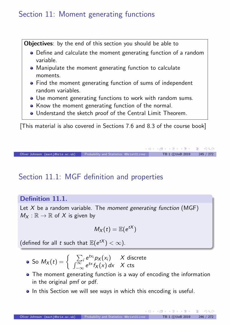
Section 11: Moment generating functions
Objectives: by the end of this section you should be able to
Define and calculate the moment generating function of a randomvariable.Manipulate the moment generating function to calculatemoments.Find the moment generating function of sums of independentrandom variables.Use moment generating functions to work with random sums.Know the moment generating function of the normal.Understand the sketch proof of the Central Limit Theorem.
[This material is also covered in Sections 7.6 and 8.3 of the course book]
Oliver Johnson ([email protected]) Probability and Statistics: @BristOliver TB 1 c©UoB 2019 245 / 272
Section 11.1: MGF definition and properties
Definition 11.1.
Let X be a random variable. The moment generating function (MGF)MX : R→ R of X is given by
MX (t) = E(etX )
(defined for all t such that E(etX ) <∞).
So MX (t) =
∑i e
txipX (xi ) X discrete∫∞−∞ etx fX (x) dx X cts
The moment generating function is a way of encoding the informationin the original pmf or pdf.
In this Section we will see ways in which this encoding is useful.
Oliver Johnson ([email protected]) Probability and Statistics: @BristOliver TB 1 c©UoB 2019 246 / 272

Example: geometric
Example 11.2.
Consider X ∼ Geom(p)
MX (t) =∞∑x=1
etxp(1− p)x−1
=∞∑x=1
pet((1− p)et
)x−1
= pet∞∑y=0
((1− p)et
)y=
pet
1− (1− p)etdefined for (1− p)et < 1
Oliver Johnson ([email protected]) Probability and Statistics: @BristOliver TB 1 c©UoB 2019 247 / 272
Example: Poisson
Example 11.3.
Consider X ∼ Poi(λ)
MX (t) =∞∑x=0
etxe−λλx
x!
= e−λ∞∑x=0
1
x!
(λet)x
= eλ(et−1).
Oliver Johnson ([email protected]) Probability and Statistics: @BristOliver TB 1 c©UoB 2019 248 / 272
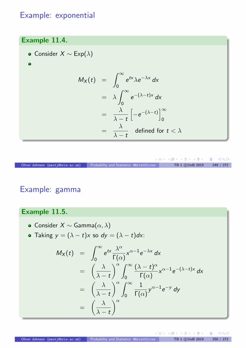
Example: exponential
Example 11.4.
Consider X ∼ Exp(λ)
MX (t) =
∫ ∞0
etxλe−λx dx
= λ
∫ ∞0
e−(λ−t)x dx
=λ
λ− t
[−e−(λ−t)
]∞0
=λ
λ− tdefined for t < λ
Oliver Johnson ([email protected]) Probability and Statistics: @BristOliver TB 1 c©UoB 2019 249 / 272
Example: gamma
Example 11.5.
Consider X ∼ Gamma(α, λ)
Taking y = (λ− t)x so dy = (λ− t)dx :
MX (t) =
∫ ∞0
etxλα
Γ(α)xα−1e−λx dx
=
(λ
λ− t
)α ∫ ∞0
(λ− t)α
Γ(α)xα−1e−(λ−t)x dx
=
(λ
λ− t
)α ∫ ∞0
1
Γ(α)yα−1e−y dy
=
(λ
λ− t
)α
Oliver Johnson ([email protected]) Probability and Statistics: @BristOliver TB 1 c©UoB 2019 250 / 272

MX uniquely defines the distribution of X .
Theorem 11.6.
Uniqueness of the MGF.
Consider random variables X , Y such that that MX (t) and MY (t) arefinite on an interval I ⊆ R containing the origin.
Suppose thatMX (t) = MY (t) for all t ∈ I .
Then X and Y have the same distribution.
Proof.
Not given.
Oliver Johnson ([email protected]) Probability and Statistics: @BristOliver TB 1 c©UoB 2019 251 / 272
Moments
Definition 11.7.
The rth moment of X is E(X r ).
Lemma 11.8.
For any random variable X and for any t:
MX (t) = 1 + tE(X ) +t2
2!E(X 2) +
t3
3!E(X 3) + · · · =
∞∑r=0
tr
r !E(X r )
i.e. MX “generates” the moments of X .
Oliver Johnson ([email protected]) Probability and Statistics: @BristOliver TB 1 c©UoB 2019 252 / 272

Proof of Lemma 11.8
Proof.
For any t, using the linearity of expectation:
MX (t) = E(etX )
= E[
1 + (tX ) +(tX )2
2!+
(tX )3
3!+ · · ·
]= 1 + tE(X ) +
t2
2!E(X 2) +
t3
3!E(X 3) + · · ·
Note that MX (0) = E(e0) = 1, as we’d expect.
Oliver Johnson ([email protected]) Probability and Statistics: @BristOliver TB 1 c©UoB 2019 253 / 272
Recovering moments of exponential
We can recover the moments of X from MX (t) in two ways:
Method 1 Expand MX (t) as a power series in t. The coefficient of tk isE(X k )k! .
Method 2 M(k)X (0) = E(X k), where M
(k)X denotes the kth derivative of
MX .To see this, note that
M ′X (t) = E(X ) + tE(X 2) +t2
2!E(X 3) + · · ·
M ′X (0) = E(X )
MX′′(t) = E(X 2) + tE(X 3) +
t2
2!E(X 4) + · · ·
MX′′(0) = E(X 2)
etc
Oliver Johnson ([email protected]) Probability and Statistics: @BristOliver TB 1 c©UoB 2019 254 / 272
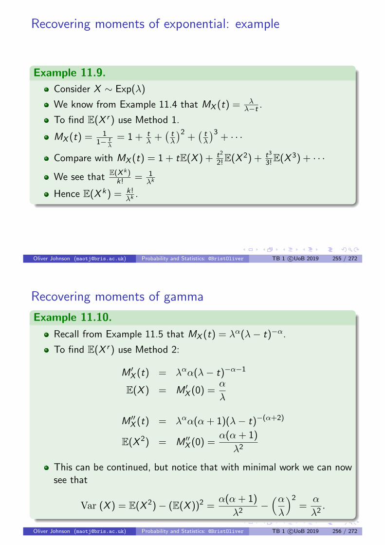
Recovering moments of exponential: example
Example 11.9.
Consider X ∼ Exp(λ)
We know from Example 11.4 that MX (t) = λλ−t .
To find E(X r ) use Method 1.
MX (t) = 11− t
λ
= 1 + tλ +
(tλ
)2+(tλ
)3+ · · ·
Compare with MX (t) = 1 + tE(X ) + t2
2!E(X 2) + t3
3!E(X 3) + · · ·
We see that E(X k )k! = 1
λk
Hence E(X k) = k!λk
.
Oliver Johnson ([email protected]) Probability and Statistics: @BristOliver TB 1 c©UoB 2019 255 / 272
Recovering moments of gamma
Example 11.10.
Recall from Example 11.5 that MX (t) = λα(λ− t)−α.
To find E(X r ) use Method 2:
M ′X (t) = λαα(λ− t)−α−1
E(X ) = M ′X (0) =α
λ
M ′′X (t) = λαα(α + 1)(λ− t)−(α+2)
E(X 2) = M ′′X (0) =α(α + 1)
λ2
This can be continued, but notice that with minimal work we can nowsee that
Var (X ) = E(X 2)− (E(X ))2 =α(α + 1)
λ2−(αλ
)2=
α
λ2.
Oliver Johnson ([email protected]) Probability and Statistics: @BristOliver TB 1 c©UoB 2019 256 / 272

Section 11.2: Sums of random variables
Theorem 11.11.
Let X1,X2, . . . ,Xn be independent rvs and let Z =∑n
i=1 Xi . Then
MZ (t) =n∏
i=1
MXi(t).
Proof.
Since Xi are independent, then for fixed t so are etXi (by Remark6.14).
MZ (t) = E(etZ ) = E(et(
∑ni=1 Xi)
)= E
(n∏
i=1
etXi
)
=n∏
i=1
E(etXi
)by independence
=n∏
i=1
MXi(t).
Oliver Johnson ([email protected]) Probability and Statistics: @BristOliver TB 1 c©UoB 2019 257 / 272
Example: adding Poissons
Example 11.12 (cf Theorem 6.18).
If X ∼ Poi(λ) and Y ∼ Poi(µ), we deduce using Example 11.3 andTheorem 11.11 that Z = X + Y has moment generating function
MZ (t) = MX (t)MY (t) = eλ(et−1).eµ(et−1)
= e(λ+µ)(et−1),
We deduce that (since it has the same MGF) Z ∼ Poi(λ+ µ) byTheorem 11.6.
Oliver Johnson ([email protected]) Probability and Statistics: @BristOliver TB 1 c©UoB 2019 258 / 272

Application: adding exponentials
Lemma 11.13.
Let X1,X2, . . . ,Xn be independent Exp(λ) rvs, and letZ = X1 + · · ·+ Xn.
Then
MXi(t) =
λ
λ− tfor each i = 1, . . . , n.
Thus by Theorem 11.11:
MZ (t) =
(λ
λ− t
)n
and Z ∼ Gamma(n, λ) by the uniqueness theorem (Theorem 11.6)
Oliver Johnson ([email protected]) Probability and Statistics: @BristOliver TB 1 c©UoB 2019 259 / 272
Section 11.3: Random sums
In Theorem ?? we saw how to calculate the expectation of a randomsum S
e.g. insurance company cares about the distribution of the totalclaims in a year.
What if we want the full distribution of S?
Theorem 11.14.
Consider X1,X2, . . . iid with distribution the same as X , and N is anon-negative integer-valued rv independent of the Xi . Then
S =
0 N = 0
X1 + · · ·+ XN N > 0
has MGF satisfyingMS(t) = MN(logMX (t))
Oliver Johnson ([email protected]) Probability and Statistics: @BristOliver TB 1 c©UoB 2019 260 / 272

Proof of Theorem 11.14
Proof.
Let A(n) = E(etS |N = n)
= E(et(X1+···+XN) |N = n)
= E(et(X1+···+Xn) |N = n)
= E(et(X1+···+Xn)) since the Xi s are independent of N
= E(etX1 · · · etXn)
= E(etX1) · · ·E(etXn) since the Xi s are independent
= (MX (t))n
= en log MX (t)
Thus E(etS |N) = A(N) = eN log MX (t) and by Theorem 10.4
MS(t) = E(etS) = E(E(etS |N)) = E(eN log MX (t)) = MN(logMX (t))
Oliver Johnson ([email protected]) Probability and Statistics: @BristOliver TB 1 c©UoB 2019 261 / 272
Example
Example 11.15.
Suppose the number of insurance claims in one year is N ∼ Poi(λ).
Suppose claims are IID Xi ∼ Exp(1), and these are independent of N.
Let S = X1 + X2 + · · ·+ XN be the total claim.
First by Example 11.3:
MN(t) = eλ(et−1).
We also know that MX (t) = 11−t (Example 11.4).
So
MS(t) = MN(logMX (t)) = eλ(e log MX (t)−1) = eλ(MX (t)−1)
= eλ( 11−t−1) = eλ( t
1−t).
From this we can calculate E(S), Var (S), etc.
Oliver Johnson ([email protected]) Probability and Statistics: @BristOliver TB 1 c©UoB 2019 262 / 272

Section 11.4: MGF of the normal
Example 11.16.
Let X ∼ N (0, 1).
So MX (t) =∫∞−∞ etx 1√
2πe−
x2
2 dx .
Let y = x − t. Key is that t(y + t)− (y+t)2
2 = −12
[y2 − t2
]so
MX (t) =1√2π
∫ ∞−∞
et(y+t)− (y+t)2
2 dy
=1√2π
∫ ∞−∞
e−12 [y2−t2] dy
= e12t2 1√
2π
∫ ∞−∞
e−12y2dy
= e12t2
Oliver Johnson ([email protected]) Probability and Statistics: @BristOliver TB 1 c©UoB 2019 263 / 272
MGF of the general normal
Example 11.17.
Now let Y ∼ N (µ, σ2)
Set X = Y−µσ so X ∼ N (0, 1) by Lemma 9.9.
Then Y = µ+ σX and
MY (t) = E(etY ) = E(et(µ+σX ))
= E(eµteσtX ) = eµtE(e(σt)X )
= eµtMX (σt) = eµte12
(σt)2
= eµt+ 12σ2t2
Oliver Johnson ([email protected]) Probability and Statistics: @BristOliver TB 1 c©UoB 2019 264 / 272

Normal distribution properties
Lemma 11.18.
1. If X ∼ N (µ, σ2) and c is a constant then X + c ∼ N (µ+ c , σ2).
2. If X ∼ N (µ, σ2) and β is a constant then βX ∼ N (βµ, β2σ2).
3. If X and Y are independent with X ∼ N (µX , σ2X ) and
Y ∼ N (µY , σ2Y ) then
X + Y ∼ N (µX + µY , σ2X + σ2
Y ).
Note: Properties 1 and 2 can easily be shown using transformation ofvariables. We use MGFs to prove all three here.
Oliver Johnson ([email protected]) Probability and Statistics: @BristOliver TB 1 c©UoB 2019 265 / 272
Proof of Lemma 11.18
Proof.
1. Let Y = X + c. Then
MY (t) = E(etY ) = E(et(X+c)) = etcE(etX ) = etcMX (t)
= etceµt+ 12σ2t2
= e(µ+c)t+ 12σ2t2
So Y ∼ N (µ+ c , σ2) by uniqueness, Theorem 11.6.
Oliver Johnson ([email protected]) Probability and Statistics: @BristOliver TB 1 c©UoB 2019 266 / 272

Proof of Lemma 11.18 (cont).
Proof.
2. Let Y = βX . Then
MY (t) = E(etY ) = E(etβX ) = MX (βt)
= eµβt+ 12σ2(βt)2
= eµβt+ 12β2σ2t2
So Y ∼ N (βµ, β2σ2) by uniqueness, Theorem 11.6.
3. Let Z = X + Y . Then by Theorem 11.11
MZ (t) = MX (t)MY (t)
= eµX t+ 12σ2X t
2eµY t+ 1
2σ2Y t2
= e(µX +µY )t+ 12
(σ2X +σ2
Y )t2
So Z ∼ N (µX + µY , σ2X + σ2
Y ) by uniqueness, Theorem 11.6.
Oliver Johnson ([email protected]) Probability and Statistics: @BristOliver TB 1 c©UoB 2019 267 / 272
Example: heights
Example 11.19.
Heights of male students are N (175, 33) and heights of femalestudents are N (170, 25).
One female and three male students are chosen at random.
What is the probability that the female is taller than the averageheight of the three males?
Let X1,X2,X3 be the height of the three male students, and Y be theheight of the female student.
We have Xi ∼ N (175, 33) and Y ∼ N (170, 25).
By Lemma 11.18.3,X1 + X2 + X3 ∼ N (175 + 175 + 175, 33 + 33 + 33).
Oliver Johnson ([email protected]) Probability and Statistics: @BristOliver TB 1 c©UoB 2019 268 / 272

Example: heights (cont.)
Example 11.19.
Let W = X1+X2+X33 be the average height of the male students. By
Lemma 11.18.2
W ∼ N
(1
3(3× 175),
(1
3
)2
(3× 33)
)= N (175, 11).
Let the difference D = Y −W = Y + (−W ).
We know Y ∼ N (170, 25), and (−W ) ∼ N (−175, 11) by Lemma11.18.2.
So D ∼ N (170 + (−175), 25 + 11) by Lemma 11.18.3, i.e.D ∼ N (−5, 36) or D+5
6 ∼ N (0, 1).
We want to know P(D > 0) = P(D+56 > 5
6 ) = 1− Φ( 56 ). Using tables
or R we can find Φ( 56 ) = 0.7976, so P(D > 0) = 1− 0.7976 = 0.2024.
Oliver Johnson ([email protected]) Probability and Statistics: @BristOliver TB 1 c©UoB 2019 269 / 272
Section 11.5: Central Limit Theorem
Consider IID X1, . . . ,Xn with mean µ and variance σ2.
The Weak Law of Large Numbers (Theorem 7.20) tells us that1n (X1 + . . .+ Xn) ' µ or X1 + . . .+ Xn − nµ ' 0.
The Central Limit Theorem tells us how close these two quantities are(the approximate distribution of the difference).
We start with an auxiliary proposition without proof.
Proposition 11.20.
Suppose MZn(t)→ MZ (t) for every t in an open interval containing 0.
Then distribution functions converge: FZn(z)→ FZ (z).
Oliver Johnson ([email protected]) Probability and Statistics: @BristOliver TB 1 c©UoB 2019 270 / 272

Central Limit Theorem
Theorem 11.21 (Central Limit Theorem (CLT)).
Let X1,X2, . . . be IID random variables with both their mean µ andvariance σ2 finite. Then for every real a < b:
limn→∞
P(a <
X1 + X2 + . . .+ Xn − nµ√nσ2
< b
)= Φ(b)− Φ(a).
Remark 11.22.
Notice that X1 + . . .+ Xn has mean nµ and variance nσ2.
CLT implies that for large n, the X1 + . . .+ Xn ' N(nµ, nσ2) orequivalently 1√
nσ2(X1 + . . .+ Xn − nµ) ' N(0, 1).
If Xi ∼ Bernoulli(p) this reduces to the de Moivre–Laplace Theorem9.11
Oliver Johnson ([email protected]) Probability and Statistics: @BristOliver TB 1 c©UoB 2019 271 / 272
Sketch proof.
Will just consider the case µ = 0, σ2 = 1 for brevity.
Write MX for the MGF of each Xi .
Know that MX (t) = 1 + 12 t
2 + O(t3).
Consider Tn :=∑n
i=1Xi√n
. Its moment generating function is
MTn(t) = E(e
t√n
∑ni=1 Xi
)= E
(n∏
i=1
et√nXi
)=
n∏i=1
E(e
t√nXi)
=n∏
i=1
MXi
(t√n
)=
[MX
(t√n
)]n=
(1 +
1
2
t2
n+ O(n−3/2)
)n
→ et2/2,
as required.
Oliver Johnson ([email protected]) Probability and Statistics: @BristOliver TB 1 c©UoB 2019 272 / 272