Steven N. Evans

Probability and Real Trees

Ecole d’Ete de Probabilites

de Saint-Flour XXXV–2005

Editor: J. Picard

December 7, 2006

Springer

Foreword

The Saint-Flour Probability Summer School was founded in 1971. It is sup-ported by CNRS, the “Ministere de la Recherche”, and the “Universite BlaisePascal”.

Three series of lectures were given at the 35th School (July 6–23, 2005) bythe Professors Doney, Evans and Villani. These courses will be published sep-arately, and this volume contains the course of Professor Evans. We cordiallythank the author for the stimulating lectures he gave at the school, and forthe redaction of these notes.

53 participants have attended this school. 36 of them have given a shortlecture. The lists of participants and of short lectures are enclosed at the endof the volume.

Here are the references of Springer volumes which have been publishedprior to this one. All numbers refer to the Lecture Notes in Mathematicsseries, except S-50 which refers to volume 50 of the Lecture Notes in Statisticsseries.

1971: vol 307 1980: vol 929 1990: vol 1527 1997: vol 17171973: vol 390 1981: vol 976 1991: vol 1541 1998: vol 17381974: vol 480 1982: vol 1097 1992: vol 1581 1999: vol 17811975: vol 539 1983: vol 1117 1993: vol 1608 2000: vol 18161976: vol 598 1984: vol 1180 1994: vol 1648 2001: vol 1837 & 18511977: vol 678 1985/86/87: vol 1362 & S-50 2002: vol 1840 & 18751978: vol 774 1988: vol 1427 1995: vol 1690 2003: vol 18691979: vol 876 1989: vol 1464 1996: vol 1665 2004: vol 1878 & 1879

Further details can be found on the summer school web sitehttp://math.univ-bpclermont.fr/stflour/

Jean PicardClermont-Ferrand, December 2006

For Ailan Hywel, Ciaran Leuel and Huw Rhys

Preface

These are notes from a series of ten lectures given at the Saint–Flour Proba-bility Summer School, July 6 – July 23, 2005.

The research that led to much of what is in the notes was supported inpart by the U.S. National Science Foundation, most recently by grant DMS-0405778, and by a Miller Institute for Basic Research in Science ResearchProfessorship.

Some parts of these notes were written during a visit to the Pacific Institutefor the Mathematical Sciences in Vancouver, Canada. I thank my long-timecollaborator Ed Perkins for organizing that visit and for his hospitality. Otherportions appeared in a graduate course I taught in Fall 2004 at Berkeley. Ithank Rui Dong for typing up that material and the students who took thecourse for many useful comments. Judy Evans, Richard Liang, Ron Peled,Peter Ralph, Beth Slikas, Allan Sly and David Steinsaltz kindly proof-readvarious parts of the manuscript.

I am very grateful to Jean Picard for all his work in organizing the Saint–Flour Summer School and to the other participants of the School, particularlyChristophe Leuridan, Cedric Villani and Matthias Winkel, for their interestin my lectures and their suggestions for improving the notes.

I particularly acknowledge my wonderful collaborators over the yearswhose work with me appears here in some form: David Aldous, Martin Barlow,Peter Donnelly, Klaus Fleischmann, Tom Kurtz, Jim Pitman, Richard Sowers,Anita Winter, and Xiaowen Zhou. Lastly, I thank my friend and collaboratorPersi Diaconis for advice on what to include in these notes.

Berkeley, California, U.S.A. Steven N. EvansOctober 2006

Contents

1 Introduction . . . . . . . . . . . . . . . . . . . . . . . . . . . . . . . . . . . . . . . . . . . . . . . 1

2 Around the continuum random tree . . . . . . . . . . . . . . . . . . . . . . . 92.1 Random trees from random walks . . . . . . . . . . . . . . . . . . . . . . . . . 9

2.1.1 Markov chain tree theorem . . . . . . . . . . . . . . . . . . . . . . . . . 92.1.2 Generating uniform random trees . . . . . . . . . . . . . . . . . . . . 13

2.2 Random trees from conditioned branching processes . . . . . . . . . 152.3 Finite trees and lattice paths . . . . . . . . . . . . . . . . . . . . . . . . . . . . . . 162.4 The Brownian continuum random tree . . . . . . . . . . . . . . . . . . . . . 172.5 Trees as subsets of `1 . . . . . . . . . . . . . . . . . . . . . . . . . . . . . . . . . . . . 18

3 R-trees and 0-hyperbolic spaces . . . . . . . . . . . . . . . . . . . . . . . . . . . . 213.1 Geodesic and geodesically linear metric spaces . . . . . . . . . . . . . . 213.2 0-hyperbolic spaces . . . . . . . . . . . . . . . . . . . . . . . . . . . . . . . . . . . . . . 233.3 R-trees . . . . . . . . . . . . . . . . . . . . . . . . . . . . . . . . . . . . . . . . . . . . . . . . . 26

3.3.1 Definition, examples, and elementary properties . . . . . . . 263.3.2 R-trees are 0-hyperbolic . . . . . . . . . . . . . . . . . . . . . . . . . . . . 323.3.3 Centroids in a 0-hyperbolic space . . . . . . . . . . . . . . . . . . . . 333.3.4 An alternative characterization of R-trees . . . . . . . . . . . . 363.3.5 Embedding 0-hyperbolic spaces in R-trees . . . . . . . . . . . . 363.3.6 Yet another characterization of R-trees . . . . . . . . . . . . . . . 38

3.4 R–trees without leaves . . . . . . . . . . . . . . . . . . . . . . . . . . . . . . . . . . . 393.4.1 Ends . . . . . . . . . . . . . . . . . . . . . . . . . . . . . . . . . . . . . . . . . . . . . 393.4.2 The ends compactification . . . . . . . . . . . . . . . . . . . . . . . . . . 423.4.3 Examples of R-trees without leaves . . . . . . . . . . . . . . . . . . 44

4 Hausdorff and Gromov–Hausdorff distance . . . . . . . . . . . . . . . . 454.1 Hausdorff distance . . . . . . . . . . . . . . . . . . . . . . . . . . . . . . . . . . . . . . . 454.2 Gromov–Hausdorff distance . . . . . . . . . . . . . . . . . . . . . . . . . . . . . . . 47

4.2.1 Definition and elementary properties . . . . . . . . . . . . . . . . . 474.2.2 Correspondences and ε-isometries . . . . . . . . . . . . . . . . . . . . 48

XII Contents

4.2.3 Gromov–Hausdorff distance for compact spaces . . . . . . . 504.2.4 Gromov–Hausdorff distance for geodesic spaces . . . . . . . . 52

4.3 Compact R-trees and the Gromov–Hausdorff metric . . . . . . . . . 534.3.1 Unrooted R-trees . . . . . . . . . . . . . . . . . . . . . . . . . . . . . . . . . . 534.3.2 Trees with four leaves . . . . . . . . . . . . . . . . . . . . . . . . . . . . . . 534.3.3 Rooted R-trees . . . . . . . . . . . . . . . . . . . . . . . . . . . . . . . . . . . . 554.3.4 Rooted subtrees and trimming . . . . . . . . . . . . . . . . . . . . . . 584.3.5 Length measure on R-trees . . . . . . . . . . . . . . . . . . . . . . . . . 59

4.4 Weighted R-trees . . . . . . . . . . . . . . . . . . . . . . . . . . . . . . . . . . . . . . . . 63

5 Root growth with re-grafting . . . . . . . . . . . . . . . . . . . . . . . . . . . . . . 695.1 Background and motivation . . . . . . . . . . . . . . . . . . . . . . . . . . . . . . . 695.2 Construction of the root growth with re-grafting process . . . . . . 71

5.2.1 Outline of the construction . . . . . . . . . . . . . . . . . . . . . . . . . 715.2.2 A deterministic construction . . . . . . . . . . . . . . . . . . . . . . . . 725.2.3 Putting randomness into the construction . . . . . . . . . . . . 765.2.4 Feller property . . . . . . . . . . . . . . . . . . . . . . . . . . . . . . . . . . . . 78

5.3 Ergodicity, recurrence, and uniqueness . . . . . . . . . . . . . . . . . . . . . 795.3.1 Brownian CRT and root growth with re-grafting . . . . . . 795.3.2 Coupling . . . . . . . . . . . . . . . . . . . . . . . . . . . . . . . . . . . . . . . . . 825.3.3 Convergence to equilibrium . . . . . . . . . . . . . . . . . . . . . . . . . 835.3.4 Recurrence . . . . . . . . . . . . . . . . . . . . . . . . . . . . . . . . . . . . . . . 835.3.5 Uniqueness of the stationary distribution . . . . . . . . . . . . . 84

5.4 Convergence of the Markov chain tree algorithm . . . . . . . . . . . . . 85

6 The wild chain and other bipartite chains . . . . . . . . . . . . . . . . . . 876.1 Background . . . . . . . . . . . . . . . . . . . . . . . . . . . . . . . . . . . . . . . . . . . . . 876.2 More examples of state spaces . . . . . . . . . . . . . . . . . . . . . . . . . . . . . 906.3 Proof of Theorem 6.4 . . . . . . . . . . . . . . . . . . . . . . . . . . . . . . . . . . . . 926.4 Bipartite chains . . . . . . . . . . . . . . . . . . . . . . . . . . . . . . . . . . . . . . . . . 956.5 Quotient processes . . . . . . . . . . . . . . . . . . . . . . . . . . . . . . . . . . . . . . . 996.6 Additive functionals . . . . . . . . . . . . . . . . . . . . . . . . . . . . . . . . . . . . . 1006.7 Bipartite chains on the boundary . . . . . . . . . . . . . . . . . . . . . . . . . . 101

7 Diffusions on a R-tree without leaves: snakes and spiders . . 1057.1 Background . . . . . . . . . . . . . . . . . . . . . . . . . . . . . . . . . . . . . . . . . . . . . 1057.2 Construction of the diffusion process . . . . . . . . . . . . . . . . . . . . . . . 1067.3 Symmetry and the Dirichlet form . . . . . . . . . . . . . . . . . . . . . . . . . . 1087.4 Recurrence, transience, and regularity of points . . . . . . . . . . . . . 1137.5 Examples . . . . . . . . . . . . . . . . . . . . . . . . . . . . . . . . . . . . . . . . . . . . . . . 1147.6 Triviality of the tail σ–field . . . . . . . . . . . . . . . . . . . . . . . . . . . . . . 1157.7 Martin compactification and excessive functions . . . . . . . . . . . . . 1167.8 Probabilistic interpretation of the Martin compactification . . . . 1227.9 Entrance laws . . . . . . . . . . . . . . . . . . . . . . . . . . . . . . . . . . . . . . . . . . . 1237.10 Local times and semimartingale decompositions . . . . . . . . . . . . . 125

Contents XIII

8 R–trees from coalescing particle systems . . . . . . . . . . . . . . . . . . . 1298.1 Kingman’s coalescent . . . . . . . . . . . . . . . . . . . . . . . . . . . . . . . . . . . . 1298.2 Coalescing Brownian motions . . . . . . . . . . . . . . . . . . . . . . . . . . . . . 132

9 Subtree prune and re-graft . . . . . . . . . . . . . . . . . . . . . . . . . . . . . . . . 1439.1 Background . . . . . . . . . . . . . . . . . . . . . . . . . . . . . . . . . . . . . . . . . . . . . 1439.2 The weighted Brownian CRT . . . . . . . . . . . . . . . . . . . . . . . . . . . . . 1449.3 Campbell measure facts . . . . . . . . . . . . . . . . . . . . . . . . . . . . . . . . . . 1469.4 A symmetric jump measure . . . . . . . . . . . . . . . . . . . . . . . . . . . . . . . 1549.5 The Dirichlet form . . . . . . . . . . . . . . . . . . . . . . . . . . . . . . . . . . . . . . . 157

A Summary of Dirichlet form theory . . . . . . . . . . . . . . . . . . . . . . . . . 163A.1 Non-negative definite symmetric bilinear forms . . . . . . . . . . . . . . 163A.2 Dirichlet forms . . . . . . . . . . . . . . . . . . . . . . . . . . . . . . . . . . . . . . . . . . 163A.3 Semigroups and resolvents . . . . . . . . . . . . . . . . . . . . . . . . . . . . . . . . 166A.4 Generators . . . . . . . . . . . . . . . . . . . . . . . . . . . . . . . . . . . . . . . . . . . . . 167A.5 Spectral theory . . . . . . . . . . . . . . . . . . . . . . . . . . . . . . . . . . . . . . . . . . 167A.6 Dirichlet form, generator, semigroup, resolvent correspondence 168A.7 Capacities . . . . . . . . . . . . . . . . . . . . . . . . . . . . . . . . . . . . . . . . . . . . . . 169A.8 Dirichlet forms and Hunt processes . . . . . . . . . . . . . . . . . . . . . . . . 169

B Some fractal notions . . . . . . . . . . . . . . . . . . . . . . . . . . . . . . . . . . . . . . . 171B.1 Hausdorff and packing dimensions . . . . . . . . . . . . . . . . . . . . . . . . . 171B.2 Energy and capacity . . . . . . . . . . . . . . . . . . . . . . . . . . . . . . . . . . . . . 172B.3 Application to trees from coalescing partitions . . . . . . . . . . . . . . 173

References . . . . . . . . . . . . . . . . . . . . . . . . . . . . . . . . . . . . . . . . . . . . . . . . . . . . . 177

Index . . . . . . . . . . . . . . . . . . . . . . . . . . . . . . . . . . . . . . . . . . . . . . . . . . . . . . . . . . 185

List of participants . . . . . . . . . . . . . . . . . . . . . . . . . . . . . . . . . . . . . . . . . . . . 187

List of short lectures . . . . . . . . . . . . . . . . . . . . . . . . . . . . . . . . . . . . . . . . . . . 191

1

Introduction

The Oxford English Dictionary provides the following two related definitionsof the word phylogeny :

1. The pattern of historical relationships between species or other groupsresulting from divergence during evolution.

2. A diagram or theoretical model of the sequence of evolutionary divergenceof species or other groups of organisms from their common ancestors.

In short, a phylogeny is the “family tree” of a collection of units designatedgenerically as taxa. Figure 1.1 is a simple example of a phylogeny for fourprimate species. Strictly speaking, phylogenies need not be trees. For instance,biological phenomena such as hybridization and horizontal gene transfer canlead to non-tree-like reticulate phylogenies for organisms. However, we willonly be concerned with trees in these notes.

Phylogenetics (that is, the construction of phylogenies) is now a huge en-terprise in biology, with several sophisticated computer packages employedextensively by researchers using massive amounts of DNA sequence data tostudy all manner of organisms. An introduction to the subject that is accessi-ble to mathematicians is [67], while many of the more mathematical aspectsare surveyed in [125].

It is often remarked that a tree is the only illustration Charles Darwinincluded in The Origin of Species. What is less commonly noted is that Dar-win acknowledged the prior use of trees as representations of evolutionaryrelationships in historical linguistics – see Figure 1.2. A recent collection ofpapers on the application of computational phylogenetic methods to historicallinguistics is [69].

The diversity of life is enormous. As J.B.S Haldane often remarked 1 invarious forms:1 See Stephen Jay Gould’s essay “A special fondness for beetles” in his book [77]

for a discussion of the occasions on which Haldane may or may not have madethis remark.

2 1 Introduction

Orangutan Gorilla Chimpanzee Human

Fig. 1.1. The phylogeny of four primate species. Illustrations are from the Tree ofLife Web Project at the University of Arizona

I don’t know if there is a God, but if He exists He must be inordinatelyfond of beetles.

Thus, phylogenetics leads naturally to the consideration of very large trees– see Figure 1.3 for a representation of what the phylogeny of all organ-isms might look like and browse the Tree of Life Web Project web-site athttp://www.tolweb.org/tree/ to get a feeling for just how large the phylo-genies of even quite specific groups (for example, beetles) can be.

Not only can phylogenetic trees be very large, but the number of possiblephylogenetic trees for even a moderate number of taxa is enormous. Phyloge-netic trees are typically thought of as rooted bifurcating trees with only theleaves labeled, and the number of such trees for n leaves is p2n3qp2n5q 7531 – see, for example, Chapter 3 of [67]. Consequently, if we tryto use statistical methods to find the “best” tree that fits a given set of data,then it is impossible to exhaustively search all possible trees and we mustuse techniques such as Bayesian Markov Chain Monte Carlo and simulatedannealing that randomly explore tree space in some way. Hence phylogeneticsleads naturally to the study of large random trees and stochastic processesthat move around spaces of large trees.

1 Introduction 3

Anatolian

Tocharian

Greek

Armenian

Italic

Celtic

Albanian

Germanic

Baltic Slavic

Vedic

Iranian

Fig. 1.2. One possible phylogenetic tree for the Indo-European family of languagesfrom [118]

Although the investigation of random trees has a long history stretchingback to the eponymous work of Galton and Watson on branching processes,a watershed in the area was the sequence of papers by Aldous [12, 13, 10].Previous authors had considered the asymptotic behavior of numerical fea-tures of an ensemble of random trees such as their height, total number ofvertices, average branching degree, etc. Aldous made sense of the idea of a se-quence of trees converging to a limiting “tree-like object”, so that many suchlimit results could be read off immediately in a manner similar to the waythat limit theorems for sums of independent random variables are straight-forward consequences of Donsker’s invariance principle and known propertiesof Brownian motion. Moreover, Aldous showed that, akin to Donsker’s invari-ance principle, many different sequences of random trees have the same limit,the Brownian continuum random tree, and that this limit is essentially thestandard Brownian excursion “in disguise”.

We briefly survey Aldous’s work in Chapter 2, where we also present someof the historical development that appears to have led up to it, namely theprobabilistic proof of the Markov chain tree theorem from [21] and the algo-rithm of [17, 35] for generating uniform random trees that was inspired bythat proof. Moreover, the asymptotic behavior of the tree–generating algo-

4 1 Introduction

Bacillus coagulans

Staphylococcus aureus

Enterococcus sulfureus

Streptococcus bovis

Lactobacillus acidophilus

Spiroplasma tiaw

anense

Clostridium

butyricum

Heliobacterium

gestii

Thermoanaerobacter lacticus

Deinococcus radiodurans

Flavobacterium odoratum

Chlam

ydia pneumoniae

Fusobacterium perfoetens

Escherichia coli

Salmonella agona

Vibrio aestuarianus

Pseudomonas m

endocina

Legionella pneumophila

Neisseria gonorrhoeae

Burkholderia solanacearum

Agrobacterium vitis

Rhizobium

leguminosarum

Rickettsia m

ontana

Cam

pylobacter hyointestinalis

Helicobacter cholecystus

Desulfoacinum

infernum

Myxococcus coralloides

Spirochaeta alkalica

Spirulina subsalsa

Chlorobium

phaeovibrioides

Trichotomospora caesia

Streptomyces lavendulae

Microbacterium

lacticum

Nocardia calcarea

Corynebacterium

acetoacidophilum

Kineococcus aurantiacus

Geoderm

atophilus obscurus

Bifidobacterium catenulatum

Chloroflexus aurantiacus

Aquifex pyrophilus

Thermotoga m

aritima

Pyrodictium

occultum

Thermoproteus tenax

Thermococcus stetteri

Thermococcus fum

icolans

Methanococcus jannaschii A

Methanococcus m

aripaludis

Methanobacterium

bryantii

Methanobacterium

subterraneum

Methanosarcina siciliae

Thermoplasm

a acidophilum

Halobacterium

marism

ortui

Haloferax denitrificans

Coem

ansia reversa

Spirodactylon aureum

Coem

ansia braziliensis

Dipsacom

yces acuminosporus

Linderina pennispora

Kickxella alabastrina

Martensiom

yces pterosporus

Sm

ittium culisetae

Capniom

yces stellatus

Furculomyces boom

erangus

Genistelloides hibernus

Spirom

yces aspiralis

Spirom

yces minutus

Conidiobolus throm

boides

Macrobiotophthora verm

icola

Strongw

ellsea castrans

Pandora neoaphidis

Zoophthora culisetae

Zoophthora radicans

Eryniopsis ptycopterae

Entom

ophaga aulicae

Entom

ophthora muscae

Entom

ophthora schizophora

Conidiobolus coronatus

Mucor ram

annianus

Mucor m

ucedo

Mucor racem

osus

Syncephalastrum

racemosum

Basidiobolus ranarum

Endogone pisiform

is

Mortierella polycephala

Acaulospora rugosa

Acaulospora spinosa

Entrophospora colum

biana

Glom

us mosseae

Glom

us cf geosporum

Glom

us mossae

Glom

us manihotis

Glom

us intraradices

Glom

us etunicatum

Glom

us claroideum

Glom

us versiforme

Scuttellospora pellucida

Scutellospora castanea

Scutellospora heterogam

a

Scuttellospora dipapillosa

Gigaspora albida

Gigaspora m

argarita

Gigaspora decipiens

Gigaspora gigantea

Acaulospora gerdem

annii

Geosiphon pyriform

e

Aleurodiscus botryosus

Stereum

hirsutum

Gloeocystidiellum

leucoxantha

Stereum

annosum

Heterobasidion annosum

Laxitextum bicolor

Hericium

ramosum

Hericium

erinaceum

Lentinellus ursinus

Lentinellus omphalodes

Clavicorona pyxidata

Auriscalpium

vulgare

Bondarzew

ia berkeleyi

Scytinostrom

a alutum

Peniophora nuda

Echinodontium

tinctorium

Russula com

pacta

Inonotus hispidus

Phellinus igniarius

Trichaptum biform

e

Trichaptum abietinum

Trichaptum fusco violaceum

Trichaptum laricinum

Basidioradulum

radula

Coltricia perennis

Schizopora paradoxa

Hyphodontia alutaria

Sphaerobolus stellatus

Geastrum

saccatum

Ram

aria stricta

Clavariadelphus pistillaris

Gom

phus floccosus

Pseudocolus fusiform

is

Auricularia polytricha

Auricularia auricula

Pseudohydnum

gelatinosum

Boletus satanas

Xerocom

us chrysenteron

Calostom

a ravenelii

Calostom

a cinnabarinum

Scleroderm

a citrina

Paxillus panuoides

Leucoagaricus gongylophorus

Basid sym

b of Atta cephalotes

Basid sym

b of Sericom

yrmex bond

Basid sym

b of Trachymyrm

ex bugn

Basid sym

b of Cyphom

yrmex rim

os

Basid sym

b of Apterostigm

a coll

Athelia bom

bacina

Panellus stipticus

Typhula phacorrhiza

Panellus serotinus

Tricholoma m

atsutake

Om

phalina umbellifera

Pleurotus ostreatus

Coprinus cinereus

Cortinarius iodes

Lepiota procera

Crucibulum

laeve

Stropharia rugosoannulata

Calvatia gigantea

Cyathus striatus

Lentinula lateritia

Am

anita muscaria

Cantharellus tubaeform

is

Dictyonem

a pavonia

Schizophyllum

comm

une

Fistulina hepatica

Pleurotus tuberregium

Agaricus bisporus

Tulostoma m

acrocephala

Pluteus petasatus

Termitom

yces cartilagineus

Termitom

yces albuminosus

Ceriporia purpurea

Bjerkandera adusta

Phlebia radiata

Phanerochaete chrysosporium

Rhizoctonia zeae

Tretopileus sphaerophorus

Dentocorticium

sulphurellum

Fomes fom

entarius

Lentinus tigrinus

Ganoderm

a australe

Trametes suaveolens

Polyporus squam

osus

Laetiporus sulphureus

Phaeolus schw

einitzii

Sparassis spathulata

Antrodia carbonica

Daedalea quercina

Fomitopsis pinicola

Spongipellis unicolor

Panus rudis

Meripilus giganteus

Albatrellus syringae

Gloeophyllum

sepiarium

Hydnum

repandum

Multiclavula m

ucida

Clavulina cristata

Botryobasidium

subcoronatum

Botryobasidium

isabellinum

Thanatephorus cucumeris

Thanatephorus praticola

Heterotextus alpinus

Calocera cornea

Dacrym

yces chrysospermus

Dacrym

yces stillatus

Tsuchiaea w

ingfieldiiC

ryptococcus neoformans

Filobasidiella neoformans

Bullera dendrophila

Trimorphom

yces papilionaceus

Bullera m

iyagianaB

ullera globosporaTrem

ella globosporaB

ullera pseudoalbaB

ullera penniseticolaB

ullera hannaeB

ullera albaB

ullera unicaTrem

ella moriform

isFellom

yces distyliiK

ockovaella schimae

Fellomyces ogasaw

arensisK

ockovaella phaffiiK

ockovaella machilophila

Kockovaella im

perataeK

ockovaella sacchariK

ockovaella thailandicaFellom

yces fuzhouensisFellom

yces penicillatusFellom

yces polyborusFellom

yces horovitziaeS

terigmatosporidium

polymorphum

Fibulobasidium inconspicuum

Sirobasidium

magnum

Bullera coprosm

aensisB

ullera oryzaeB

ullera derxiiB

ullera sinensisB

ullera mrakii

Bullera huiaensis

Bul

lera

cro

cea

Bul

lera

arm

enia

caB

ulle

ra v

aria

bilis

Tric

hosp

oron

cut

aneu

mTr

icho

spor

on ja

poni

cum

Trem

ella

folia

cea

Hol

term

anni

a co

rnifo

rmis

Filo

basi

dium

flor

iform

eM

raki

a ps

ychr

ophi

liaM

raki

a fri

gida

Ude

niom

yces

meg

alos

poru

sU

deni

omyc

es p

unic

eus

Ude

niom

yces

piri

cola

Bul

lera

gra

ndis

pora

Leuc

ospo

ridiu

m la

ri m

arin

iC

ysto

filob

asid

ium

cap

itatu

mP

haffi

a rh

odoz

yma

Till

etia

car

ies

Tille

tiaria

ano

mal

aT

illet

iops

is fu

lves

cens

Till

etio

psis

flav

aT

illet

iops

is m

inor

Till

etio

psis

alb

esce

ns

Till

etio

psis

was

hing

tone

nsis

Till

etio

psis

pal

lesc

ens

Ust

ilago

hor

dei

Ust

ilago

may

dis

Ust

ilago

shi

raia

naG

raph

iola

cyl

indr

ica

Gra

phio

la p

hoen

icis

Cam

ptob

asid

ium

hyd

roph

ilum

Sym

podi

omyc

opsi

s pa

phio

pedi

li

Kon

doa

mal

vine

lla

Ben

sing

toni

a m

isca

nthi

Ben

sing

toni

a su

bros

ea

Ben

sing

toni

a yu

ccic

ola

Ben

sing

toni

a ph

ylla

dus

Myc

oglo

ea m

acro

spor

a

Ste

rigm

atom

yces

hal

ophi

lus

Aga

ricos

tilbu

m h

ypha

enes

Ben

sing

toni

a in

gold

ii

Ben

sing

toni

a m

usae

Kur

tzm

anom

yces

nec

taire

i

Chi

onos

phae

ra a

poba

sidi

alis

Spo

robo

lom

yces

xan

thus

Ben

sing

toni

a na

gano

ensi

s

Ben

sing

toni

a ci

liata

Mix

ia o

smun

dae

Rho

dosp

orid

ium

toru

loid

es

Rho

doto

rula

glu

tinis

Rho

doto

rula

gra

min

is

Rho

doto

rula

muc

ilagi

nosa

Rho

dosp

orid

ium

fluv

iale

Spo

ridio

bolu

s jo

hnso

nii

Spo

robo

lom

yces

rose

us

Ben

sing

toni

a ya

mat

oana

Zym

oxen

oglo

ea e

rioph

ori

Mic

robo

tryum

vio

lace

um

Leuc

ospo

ridiu

m s

cotti

i

Ben

sing

toni

a in

term

edia

Het

erog

astri

dium

pyc

nidi

oide

um

Hya

lops

ora

poly

podi

i

Per

ider

miu

m h

arkn

essi

i

Cro

narti

um ri

bico

la

Ure

dino

psis

inte

rmed

ia

Phy

sope

lla a

mpe

lops

idis

Gym

noco

nia

nite

ns

Puc

cini

a su

zuta

ke

Nys

sops

ora

echi

nata

Aec

idiu

m e

pim

edii

Rho

doto

rula

min

uta

Ery

thro

basi

dium

has

egaw

ianu

m

Rho

doto

rula

lact

osa

Rho

dosp

orid

ium

dac

ryoi

dum

Hel

icob

asid

ium

pur

pure

um

Hel

icob

asid

ium

mom

pa

Hel

icob

asid

ium

cor

ticio

ides

Hel

icog

loea

var

iabi

lis

Gra

phiu

m p

utre

dini

s

Gra

phiu

m te

cton

ae

Pet

riella

set

ifera

Lom

ento

spor

a pr

olifi

cans

Pse

udal

lesc

heria

boy

dii

Pse

udal

lesc

heria

elli

psoi

dea

Lign

inco

la la

evis

Nai

s in

orna

ta

Ani

ptod

era

ches

apea

kens

is

Hal

osar

phei

a re

torq

uens

Mic

roas

cus

cirr

osus

Gra

phiu

m p

enic

illioi

des

Cer

atoc

ystis

fim

bria

ta

Fusa

rium

cul

mor

um

Gib

bere

lla p

ulic

aris

Fusa

rium

cer

ealis

Fusa

rium

equ

iset

i

Nec

tria

haem

atoc

occa

Fusa

rium

oxy

spor

um

Gib

bere

lla a

vena

cea

Fusa

rium

mer

ism

oide

s

Pae

cilo

myc

es te

nuip

es

Cor

dyce

pioi

deus

bis

poru

s

Ham

ilton

aphi

s st

yrac

i sym

b

Geo

smith

ia p

utte

rillii

Geo

smith

ia la

vend

ula

Spi

cellu

m ro

seum

Myc

oara

chis

inve

rsa

Nec

tria

ochr

oleu

ca

Nec

tria

aure

oful

va

Cha

etop

sina

fulv

a

Hyp

ocre

a lu

tea

Hyp

omyc

es c

hrys

ospe

rmus

Glo

mer

ella

cin

gula

ta

Vert

icill

ium

dah

liae

Hyp

oxyl

on fr

agifo

rme

Xyl

aria

car

poph

ila

Xyl

aria

pol

ymor

pha

Ros

ellin

ia n

ecat

rix

Obo

larin

a dr

yoph

ila

Kio

noch

aeta

ivor

iens

is

Kio

noch

aeta

spi

ssa

Kio

noch

aeta

ram

ifera

Mel

iola

judd

iana

Mel

iola

nie

ssle

ana

Podo

spor

a an

serin

a

Neu

rosp

ora

cras

sa

Sor

daria

fim

icol

a

Cha

etom

ium

ela

tum

Cam

arop

s m

icro

spor

a

Asc

ovag

inos

pora

ste

llipal

a

Cry

phon

ectri

a pa

rasi

tica

Cry

phon

ectri

a ra

dica

lis

Cry

phon

ectri

a ha

vane

nsis

Cry

phon

ectri

a cu

bens

is

End

othi

a gy

rosa

Leuc

osto

ma

pers

ooni

i

Oph

iost

oma

euro

phio

ides

Oph

iost

oma

cucu

llatu

m

Oph

iost

oma

aino

ae

Oph

iost

oma

sten

ocer

as

Spo

roth

rix s

chen

ckii

Oph

iost

oma

ulm

i

Oph

iost

oma

peni

cilla

tum

Peso

tum

frag

rans

Oph

iost

oma

bico

lor

Oph

iost

oma

pice

ae

Pse

udoh

alon

ectri

a fa

lcat

a

Oph

ioce

ras

lept

ospo

rum

Mag

napo

rthe

gris

ea

Lulw

orth

ia fu

cico

la

Spa

thul

aria

flav

ida

Cud

onia

con

fusa

Rhy

tism

a sa

licin

um

Mon

ilinia

laxa

Mon

ilinia

fruc

ticol

a

Scl

erot

inia

scl

erot

ioru

m

Am

yloc

arpu

s en

ceph

aloi

des

Neo

bulg

aria

pre

mno

phila

Blu

mer

ia g

ram

inis

Phy

llact

inia

gut

tata

Cyt

taria

dar

win

ii

Thel

ebol

us s

terc

oreu

s

Asc

ozon

us w

oolh

open

sis

Leot

ia lu

bric

a

Mic

rogl

ossu

m v

iride

Geo

myc

es p

anno

rum

Geo

myc

es p

anno

rum

var

asp

erul

a

Bul

garia

inqu

inan

s

Lept

osph

aeria

bic

olor

Cuc

urbi

doth

is p

ityop

hila

Kirs

chst

eini

othe

lia e

late

rasc

us

Hel

icas

cus

kana

loan

us

Pyr

enop

hora

tric

host

oma

Pyr

enop

hora

triti

ci re

pent

is

Coc

hlio

bolu

s sa

tivus

Alte

rnar

ia b

rass

icae

Cla

thro

spor

a di

plos

pora

Alte

rnar

ia a

ltern

ata

Alte

rnar

ia b

rass

icic

ola

Alte

rnar

ia ra

phan

i

Pleo

spor

a he

rbar

um

Set

osph

aeria

rost

rata

Ple

ospo

ra b

etae

Lept

osph

aeria

dol

iolu

m

Lept

osph

aeria

mac

ulan

s

Cuc

urbi

taria

elo

ngat

a

Lept

osph

aeria

mic

rosc

opic

a

Oph

iobo

lus

herp

otric

hus

Phae

osph

aeria

nod

orum

Cuc

urbi

taria

ber

berid

is

Ple

ospo

ra ru

dis

Wes

terd

ykel

la d

ispe

rsa

Loph

iost

oma

cren

atum

Spo

rom

ia li

gnic

ola

Mon

odic

tys

cast

anea

e

Kirs

chst

eini

othe

lia m

ariti

ma

Her

potri

chia

juni

peri

Myc

osph

aere

lla m

ycop

appi

Her

potri

chia

diff

usa

Den

dryp

hiop

sis

atra

Botry

osph

aeria

rhod

ina

Bot

ryos

phae

ria ri

bis

Pha

eosc

lera

dem

atio

ides

Dot

hide

a in

scul

pta

Dot

hide

a hi

ppop

haeo

s

Aure

obas

idiu

m p

ullu

lans

Coc

codi

nium

bar

tsch

ii

Sar

cino

myc

es c

rust

aceu

s

Sip

hula

cer

atite

s

Pertu

saria

trac

hyth

allin

a

Dip

losc

hist

es o

cella

tus

var a

l

Anam

ylop

sora

pul

cher

rima

Trap

elia

pla

codi

oide

s

Trap

elia

invo

luta

Pla

cops

is g

elid

a

Con

otre

ma

popu

loru

m

Cya

node

rmel

la v

iridu

la

Gya

lect

a ul

mi

Nep

hrom

a ar

cticu

m

Peltig

era

neop

olyd

acty

la

Solo

rina

croc

ea

Pseu

deve

rnia

cla

doni

ae

Pilo

phor

us a

cicu

laris

Cla

dia

aggr

egat

a

Cla

doni

a be

llidifl

ora

Ster

eoca

ulon

ram

ulos

um

Leca

nora

disp

ersa

Squa

mar

ina

lent

iger

a

Rhi

zoca

rpon

geo

grap

hicu

m

Spha

erop

horu

s gl

obos

us

Leifid

ium

tene

rum

Buno

doph

oron

scr

obicu

latu

m

Xant

horia

ele

gans

Meg

alos

pora

sul

phur

ata

Lecid

ea fu

scoa

tra

Porp

idia

cru

stul

ata

Cal

icium

ads

pers

um

Texo

spor

ium

san

cti ja

cobi

Thelo

mm

a m

amm

osum

Cyp

heliu

m in

quin

ans

Chr

omoc

leist

a m

alac

hite

a

Peni

cilliu

m n

otat

um

Eupe

nici

llium

cru

stac

eum

Peni

cilliu

m fr

eii

Peni

cilliu

m n

amys

low

skii

Geo

smith

ia n

amys

low

skii

Eupe

nici

llium

java

nicu

m

Mer

imbl

a in

gelh

eim

ense

Ham

iger

a av

ella

nea

Hem

icarp

ente

les

orna

tus

Aspe

rgillu

s fla

vus

Aspe

rgillu

s or

yzae

Aspe

rgillu

s no

miu

s

Aspe

rgillu

s pa

rasi

ticus

Aspe

rgillu

s ta

mar

ii

Aspe

rgillu

s so

jae

Aspe

rgillu

s av

enac

eus

Mon

ascu

s pu

rpur

eus

Euro

tium

her

bario

rum

Euro

tium

rubr

um

Aspe

rgillu

s re

stric

tus

Aspe

rgillu

s us

tus

Aspe

rgillu

s ve

rsico

lor

Emer

icella

nid

ulan

s

Aspe

rgillu

s ni

dula

ns

Fenn

ellia

flav

ipes

Aspe

rgillu

s te

rreus

Aspe

rgillu

s w

entii

Chae

tosa

rtory

a cr

emea

Neos

arto

rya

fisch

eri

Aspe

rgillu

s fu

mig

atus

Aspe

rgillu

s cla

vatu

s

Aspe

rgillu

s oc

hrac

eus

Aspe

rgillu

s ni

ger

Aspe

rgillu

s aw

amor

ii

Aspe

rgillu

s ce

rvin

us

Aspe

rgillu

s ca

ndid

us

Aspe

rgillu

s zo

natu

s

Aspe

rgillu

s sp

arsu

s

Byss

ochl

amys

nive

a

Paec

ilom

yces

var

iotii

Ther

moa

scus

crus

tace

us

Geo

smith

ia c

ylind

rosp

ora

Talar

omyc

es e

burn

eus

Talar

omyc

es e

mer

sonii

Tala

rom

yces

flavu

s

Tala

rom

yces

bac

illisp

orus

Elap

hom

yces

leve

illei

Elap

hom

yces

mac

ulat

us

Auxa

rthro

n zu

ffianu

m

Malb

ranc

hea

filam

ento

sa

Malb

ranc

hea

dend

ritica

Malb

ranc

hea

albolu

tea

Uncin

ocar

pus

rees

ii

Cocc

idio

ides

imm

itis

Ony

gena

equ

ina

Reni

spor

a fla

vissim

a

Cten

omyc

es se

rratu

s

Trich

ophy

ton

rubr

um

Gym

noas

coide

us p

etalo

spor

us

Chry

sosp

orium

par

vum

Blas

tom

yces

der

mat

itidis

Histo

plasm

a ca

psula

tum

Histop

lasm

a ca

psula

tum

ssp

farc

i

Histo

plasm

a ca

psula

tum

ssp

dubo

i

Asco

spha

era

apis

Erem

ascu

s albu

s

Malb

ranc

hea

gyps

ea

Phae

oann

ellom

yces

eleg

ans

Nads

oniel

la nig

ra

Exop

hial

a je

anse

lmei

Phae

ococ

com

yces

exo

phial

ae

Capro

nia p

ilose

lla

Exop

hiala

man

sonii

Pullu

laria

prot

otro

pha

Exop

hiala

derm

atitid

is

Sarc

inom

yces

pha

eom

urifo

rmis

Capro

nia m

anso

nii

Gra

phium

calic

ioide

s

Ceram

othy

rium

linna

eae

Conios

poriu

m a

pollin

is

Conios

poriu

m p

erfor

ans

Chaen

othe

cops

is sa

vonic

a

Sphin

ctrina

turb

inata

Sten

ocyb

e pu

llatu

la

Myc

ocali

cium

albo

nigru

m

Lasa

llia ro

ssica

Umbil

icaria

subg

labra

Steg

obium

pan

iceum

yeas

t like

sym

Lasio

derm

a se

rrico

rne

yeas

t like

Mon

acro

spor

ium el

lipso

spor

a

Orbilia

aur

icolor

Arth

robo

trys c

onoid

es

Duddin

gton

ia fla

gran

s

Mon

acro

spor

ium ge

phyro

paga

Mon

acro

spor

ium ha

ptotyl

um

Arthr

obotr

ys ro

busta

Dactyl

ella

oxys

pora

Dactyl

ella

rhop

alota

Arth

robo

trys d

actyl

oides

Orbilia

deli

catu

la

Choiro

myc

es m

eand

riform

is

Choiro

myc

es ve

nosu

s

Tube

r mag

natum

Tube

r pan

nifer

um

Tube

r exc

avatu

m

Tube

r rapa

eodo

rum

Tube

r gibb

osum

Tube

r bor

chii

Dingley

a ver

ruco

sa

Laby

rintho

myc

es va

rius

Redde

llom

yces

don

kii

Wyn

nella

silvi

color

Barss

ia or

egon

ensis

Balsam

ia vu

lgaris

Balsam

ia m

agna

ta

Helvell

a lac

unos

a

Helvell

a ter

restr

is

Under

woodia

colum

naris

Calosc

ypha

fulge

ns

Pulvinu

la ar

cher

i

Chalaz

ion he

lvetic

um

Ascod

esmis

spha

eros

pora

Glaziel

la au

ranti

aca

Aleuria

aura

ntia

Inerm

isia a

ggreg

ata

Trich

opha

ea hy

brida

Wilc

oxina

miko

lae

Scute

llinia

scut

ellat

a

Leuc

oscy

pha o

roarct

ica

Pyrone

ma dom

estic

um

Otidea

lepo

rina

Neottie

lla ru

tilans

Pauro

cotyl

is pil

a

Geopy

xis ca

rbona

ria

Tarze

tta ca

tinus

Cooke

ina su

lcipe

s

Sarcos

cyph

a aus

triaca

Micros

toma p

rotrac

ta

Desmaz

ierell

a acic

ola

Plectan

ia rhy

tidia

Sarcos

oma g

lobos

um

Urnula

hiem

alis

Morche

lla es

culen

ta

Morche

lla el

ata

Verp

a con

ica

Verpa

bohe

mica

Leuc

angiu

m carth

usian

um

Fische

rula s

ubca

ulis

Disciot

is ve

nosa

Hydno

trya t

ulasn

ei

Gyromitra

escu

lenta

Gyromitra

mela

leuco

ides

Pseud

orhizi

na ca

liforni

ca

Gyromitra

mon

tana

Discina

mac

rospo

ra

Hydno

trya c

erebri

formis

Rhizina

undu

lata

Cazia

flexia

scus

Terfe

zia ar

enari

a

Peziza

succ

osa

Peziza

quele

pidoti

a

Terfe

zia te

rfezio

ides

Pachy

phloe

us m

elano

xanth

us

Boudie

ra ac

antho

spora

Peziza

badia

Theco

theus

holm

skjol

dii

Ascob

olus l

ineola

tus

Pichia

mexica

na

Candid

a con

globa

ta

Candid

a aas

eri

Candid

a buty

ri

Candid

a ins

ector

um

Candid

a den

drone

ma

Candid

a ten

uis

Candid

a nae

oden

dra

Candid

a didd

ensia

e

Candid

a atla

ntica

Candid

a atm

osph

aeric

a

Candid

a buin

ensis

Candid

a frie

drich

ii

Candid

a mem

branifa

ciens

Pichia

triang

ularis

Candid

a mult

igemmis

Candid

a oleo

phila

Candid

a bole

ticola

Candida schatav

ii

Candid

a lau

reliae

Candida kriss

ii

Candid

a san

tamari

ae va

r mem

bra

Candid

a ralu

nens

is

Candid

a san

tamari

ae va

r san

tam

Candid

a bee

chii

Candid

a zey

lanoid

es

Candid

a sop

hiae r

egina

e

Candid

a que

rcitrus

a

Candida natalensis

Candid

a frag

i

Candida psychrophila

Candida glucoso

phila

Candida xesto

bii

Candid

a fuk

uyam

aens

is

Candid

a ferm

entica

rens

Pichia guillie

rmondii

Debaryomyce

s hanse

nii var h

ans

Debaryomyce

s hansenii v

ar fabr

Taphrina farlo

wii

Yamadazym

a guillierm

ondii

Pichia fa

rinosa

Debaryomyce

s udenii

Debaryomyce

s caste

llii

Debaryomyce

s hansenii

Candida sojae

Candida tropica

lis

Candida albicans

Candida dubliniensis

Candida maltosa

Candida viswanathii

Candida lodderae

Candida parapsilosis

Lodderomyces e

longisporus

Candida shehatae va

r insecto

sa

Candida shehatae va

r lignosa

Candida shehatae va

r shehatae

Candida palmioleophila

Candida fluvia

tilis

Candida saitoana

Candida pseudoglaebosa

Candida glaebosa

Candida insectamans

Candida lyxosophila

Candida kruisii

Candida tanzawaensis

Candida sake

Candida austromarina

Candida coipomoensis

Candida ergastensis

Pichia angusta

Williopsis

salico

rniae

Endomyces fi

buliger

Saccharomyco

psis fib

uligera

Saccharomyco

psis ca

psularis

Kluyveromyce

s nonferm

entati

Kluyveromyce

s aestu

arii

Kluyveromyce

s marxia

nus

Kluyveromyce

s lactis

Kluyveromyce

s dobzhanski

i

Kluyveromyce

s wicke

rhamii

Holleya sinecauda

Zygosaccharomyce

s mellis

Zygosaccharomyce

s rouxii

Zygosaccharomyce

s bisp

orus

Zygosaccharomyce

s lentus

Zygosaccharomyce

s bailii

Arxiozym

a telluris

Saccharomyce

s dairensis

Saccharomyce

s serva

zzii

Saccharomyce

s unisp

orus

Saccharomyce

s transva

alensis

Zygosaccharomyce

s mrakii

Torulaspora globosa

Torulaspora delbrueckii

Torulaspora pretoriensis

Zygosaccharomyce

s micro

ellipsoide

Candida colliculosa

Kazachstania viticola

Kluyveromyce

s blattae

Kluyveromyce

s phaffii

Zygosaccharomyce

s florentinus

Candida glabrata

Kluyveromyces delphensis

Saccharomyce

s pasto

rianus

Saccharomyce

s cerevisi

ae

Saccharomyce

s cerevisi

ae 2

Saccharomyce

s bayanus

Saccharomyce

s paradoxus

Kluyveromyce

s polysp

orus

Kluyveromyces yarrowii

Kluyveromyce

s lodderae

Saccharomyces rosinii

Kluyveromyces africanus

Saccharomyce

s spencerorum

Saccharomyces exiguus

Saccharomyces barnettii

Saccharomyces castellii

Zygosaccharomyce

s fermentati

Saccharomyces kluyveri

Kluyveromyces thermotolerans

Kluyveromyces waltii

Saccharomycodes ludwigii

Hanseniaspora uvarum

Williopsis pratensis

Williopsis californica

Starmera amethionina var pachy

Starmera amethionina var ameth

Starmera caribaea

Pichia anomala

Williopsis saturnus

Williopsis saturnus var mrakii

Williopsis mucosa

Pachysolen tannophilus

Candida chilensis

Candida cylindracea

Candida savonica

Candida mesenterica

Candida suecica

Phaffomyces antillensis

Phaffomyces opuntiae

Phaffomyces thermotolerans

Yarrowia lipolyticaCandida rugosa

Candida catenulata

Candida pseudointermedia

Candida intermedia

Candida akabanensis

Candida oregonensis

Candida haemulonii

Candida tsuchiyae

Clavispora lusitaniae

Candida melibiosica

Candida torresii

Metschnikowia bicuspidata

Candida agrestis

Metschnikowia reukaufii

Metschnikowia pulcherrima

Candida mogii

Brettanomyces bruxellensis

Dekkera bruxellensisDekkera anomala

Brettanomyces anomalus

Dekkera custersiana

Dekkera naardenensis

Candida insectalensCandida silvatica

Issatchenkia orientalis

Pichia membranaefaciens

Candida spandovensisCandida apicolaCandida bombi

Starmerella bombicola

Candida geocharesCandida vaccinii

Endomyces geotrichum

Galactomyces geotrichum

Dipodascus albidus

Candida chiropterorum

Candida valdivianaCandida drimydis

Waltomyces lipofer

Dipodascopsis uninucleata

Protomyces macrosporus

Protomyces pachydermusProtomyces inouyei

Protomyces lactucaeTaphrina virginicaTaphrina carnea

Taphrina pruni subcordataeTaphrina mirabilisTaphrina nana

Taphrina pruniTaphrina ulmi

Taphrina communisTaphrina flavorubraTaphrina populina

Taphrina deformansTaphrina wiesneri

Taphrina robinsonianaTaphrina letifera

Neolecta vitellinaNeolecta irregularis

Saitoella complicata

Schizosaccharomyces pombe

Schizosaccharomyces japonicusPneumocystis carinii

Calicium tricolorTaphrina maculans

Taphrina californicaChytridium confervae

Neocallimastix frontalisNeocallimastix joyoniiPiromonas communis

Spizellomyces acuminatus

Allomyces macrogynus

Blastocladiella emersoniiChrysops niger

Drosophila melanogasterCeratitis capitataOrnithoica vicina

Nephrotoma altissimaLutzomyia shannoni

Aedes albopictusAedes aegyptiAedes punctor

Toxorhynchites ambionensisCulex tritaeniorhynchus

Anopheles psuedopunctipennisAnopheles albimanus

Eucorethra underwoodiDixella cornuta

Culicoides variipennisAmblabesmia rhamphe

Simulium vittatumXenos vesparumStylops melittaeMengenilla chobautiGalleria mellonella

Archaeopsylla erinaceiPanorpa germanica

Anisochrysa carneaOliarces claraMonolobus ovalipennis

Antarctonomus complanatusLoricera foveataLoricera pilicornis pilicornis

Amarotypus edwardsiBembidion mexicanum

Bembidion levettei carrianumAsaphidion curtumDiplous californicusPatrobus longicornisPericompsus laetulusDiplochaetus planatusZolus helmsi

Merizodus angusticollisSloaneana tasmaniaeBatesiana hilarisSchizogenius falliClivina ferreaDyschirius sphaericollisMelisodera picipennisMecyclothorax vulcansAmblytelus curtusApotomus rufithoraxBroscosoma relictumCreobius eydouxiGalerita lecontei leconteiPseudaptinus rufulusAptinus displosorPterostichus melanariusTetragonoderus latipennisDiscoderus cordicollisChlaenius ruficaudaCalybe laetulaAmara apricariaAgonum extensicolleCymindis punctigeraLoxandrus n sp nr amplithoraCnemalobus sulciferusCatapiesis brasiliensisMorion aridusBrachinus armigerBrachinus hirsutusPheropsophus aequinoctialisPasimachus atronitensScarites subterraneusCarenum interruptumSiagona europaeaSiagona jennisoniClinidium calcaratumOmoglymmius hamatusOmus californicusCicindela sedecimpunctataMetrius contractusPachyteles striolaCymbionotum semelederiCymbionotum pictulumGehringia olympicaPromecognathus crassusLaccocenus ambiguusOmophron obliteratumPsydrus piceusCeroglossus chilensisPamborus gueriniiCalosoma scrutatorCarabus nemoralisScaphinotus petersi catalinae

Cychrus italicusOpisthius richardsoniLeistus ferruginosusNebria hudsonicaNotiophilus semiopacusTrachypachus gibbsiiTrachypachus holmbergiSystolosoma lateritiumElaphrus californicus

Elaphrus clairvilleiBlethisa multipunctata aurataMecodema fulgidum

Oregus aereusSuphis inflatusCopelatus chevrolati renovatusHydroscapha natans

Xanthopyga cactiDynastes grantiTenebrio molitor

Meloe proscarabaeusClambus arnetti

Phaeostigma notataLeptothorax acervorum

Polistes dominulusGraphosoma lineatumRaphigaster nebulosa

Lygus hesperusHemiowoodwardia wilsoni

Hackeriella veitchiSpissistilus festinusProkelisia marginataPhilaenus spumariusOkanagana utahensis

Trioza eugeniaePealius kelloggii

Acyrthosiphon pisumAonidiella aurantii

Batrachideidae gen spCarausius morosusAcheta domesticusMesoperlina pecircai

Aeschna cyaneaLepisma saccharina

Lepidocyrtus paradoxusCrossodonthina koreana

Hypogastrura dolsanaPodura aquatica

Theatops erythrocephalaScolopendra cingulata

Cryptops trisulcatus

Craterostigmus tasmanianusLithobius variegatus

Scutigera coleoptrata

Pseudohimantarium mediterraneum

Clinopodes poseidonis

Cylindroiulus punctatus

Polydesmus coriaceus

Rhipicephalus appendiculatus

Hyalomma lusitanicum

Hyalomma rufipes

Hyalomma dromedarii

Rhipicephalus sanguineus

Boophilus microplus

Rhipicephalus zambeziensis

Rhipicephalus bursa

Boophilus annulatus

Rhipicephalus pusillus

Dermacentor andersoni

Dermacentor marginatus

Amblyomma triguttatum triguttat

Amblyomma vikirri

Aponomma fimbriatum

Aponomma latum

Amblyomma variegatum

Amblyomma tuberculatum

Amblyomma americanum

Amblyomma maculatum

Haemaphysalis inermis

Haemaphysalis punctata

Haemaphysalis leporispalustris

Haemaphysalis humerosa

Haemaphysalis petrogalis

Haemaphysalis leachi

Aponomma undatum

Aponomma concolor

Ixodes auritulus

Ixodes ricinus

Ixodes affinis

Ixodes pilosus

Ixodes cookei

Ixodes simplex simplex

Ixodes kopsteini

Ixodes holocyclus

Carios puertoricensis

Ornithodoros moubata

Ornithodoros coriaceus

Otobius megnini

Argas lahorensis

Argas persicus

Megisthanus floridanus

Cosmolaelaps trifidus

Hypochthonius rufulus

Lohmannia banksi

Nothrus sylvestris

Xenillus tegeocranus

Euzetes globulosus

Allonothrus russeolus

Archegozetes longisetosus

Trhypochthonius tectorum

Nehypochthonius porosus

Steganacarus magnus

Gehypochthonius urticinus

Chortoglyphus arcuatus

Acarus siro

Eusimonia wunderlichi

Androctonus australis

Liphistius bicoloripes

Eurypelma californica

Odiellus troguloides

Pseudocellus pearsei

Limulus polyphemus

Callipallene gen sp

Berndtia purpurea

Trypetesa lampas

Octolasmis lowei

Paralepas palinuri

Lepas anatifera

Balanus eburneus

Chelonibia patula

Tetraclita stalactifera

Chthamalus fragilis

Verruca spengleri

Ibla cumingi

Calantica villosa

Loxothylacus texanus

Dendrogaster asterinae

Ulophysema oeresundense

Palaemonetes kadiakensis

Helice tridens

Philyra pisum

Callinectes sapidus

Pugettia quadridens

Raninoides louisianensis

Procambarus leonensis

Astacus astacus

Nephrops norvegicus

Panulirus argus

Oedignathus inermis

Penaeus aztecus

Stenopus hispidus

Artemia salina

Branchinecta packardi

Daphnia pulex

Bosmina longirostris

Daphnia galeata

Stenocypris major

Argulus nobilis

Porocephalus crotali

Milnesium tardigradum

Macrobiotus hufelandi

Thulinia stephaniae

Echiniscus viridissimus

Euperipatoides leuckarti

Priapulus caudatus

Pycnophyes kielensis

Helix aspersa

Balea biplicata

Limicolaria kambeul

Laevicaulis alte

Onchidella celtica

Siphonaria algesirae

Anthosiphonaria sirius

Lymnaea glabra

Stagnicola palustris

Lymnaea stagnalis

Radix peregra

Lymnaea auricularia

Fossaria truncatula

Bakerilymnaea cubensis

Biomphalaria glabrata

Littorina obtusata

Littorina littorea

Fasciolaria lignaria

Nassarius singuinjorensis

Pisania striata

Reishia bronni

Thais clavigera

Rapana venosa

Bursa rana

Monodonta labio

Antalis vulgaris

Scutopus ventrolineatus

Arctica islandica

Mercenaria mercenaria

Spisula subtruncata

Mulinia lateralis

Spisula solida

Spisula solidissima

Tresus nuttali

Tresus capax

Mactromeris polynyma

Hippopus hippopus

Hippopus porcellanus

Tridacna squamosa

Tridacna crocea

Tridacna maxima

Tridacna derasa

Tridacna gigas

Vasticardium flavum

Fulvia mutica

Fragum unedo

Fragum fragum

Corculum cardissa

Galeomma takii

Ostrea edulis

Crassostrea virginica

Nerita albicilla

Mytilus edulis

Mytilus trossulus

Mytilus galloprovincialis

Mytilus californianus

Geukensia demissa

Mimachlamys varia

Chlamys hastata

Crassadoma gigantea

Pecten maximus

Argopecten gibbus

Argopecten irradians

Placopecten magellanicus

Chlamys islandica

Atrina pectinata

Arca noae

Barbatia virescens

Acanthopleura japonica

Lepidochitona corrugata

Lepidozona coreanica

Eohemithyris grayii

Platidia anomioides

Stenosarina crosnieri

Gryphus vitreus

Thecidellina blochmanii

Cancellothyris hedleyi

Terebratulina retusa

Liothyrella neozelanica

Liothyrella uva

Gwynia capsula

Calloria inconspicua

Gyrothyris mawsoni

Neothyris parva

Terebratalia transversa

Macandrevia cranium

Fallax neocaledonensis

Laqueus californianus

Megerlia truncata

Terebratella sanguinea

Notosaria nigricans

Hemithyris psittaceae

Neocrania anomala

Neocrania huttoni

Discina striata

Glottidia pyramidata

Lingula lingua

Lingula anatina

Phoronis architecta

Phoronis psammophila

Phoronis vancouverensis

Alboglossiphonia heteroclita

Hirudo medicinalis

Haemopis sanguisuga

Barbronia weberi

Eisenia fetida

Lumbricus rubellus

Dero digitata

Xironogiton victoriensis

Sathodrilus attenuatus

Nereis virens

Aphrodita aculeata

Nereis limbata

Capitella capitata

Harmothoe impar

Sabella pavonina

Magelona mirabilis

Scoloplos armiger

Polydora ciliata

Pygospio elegans

Lanice conchilega

Nephtys hombergii

Glycera americana

Dodecaceria concharum

Chaetopterus variopedatus

Siboglinum fiordicum

Ridgeia piscesae

Ochetostoma erythrogrammon

Pedicellina cernua

Barentsia hildegardae

Barentsia benedeni

Symbion pandora

Plumatella repens

Alcyonidium gelatinosum

Porania pulvillus

Asterias amurensis

Astropecten irregularis

Stomopneustes variolaris

Mespilia globulus

Temnopleurus hardwickii

Salmacis sphaeroides

Tripneustes gratilla

Ophiopholis aculeta

Strongylocentrotus intermedius

Colobocentrotus atratus

Echinus esculentus

Sphaerechinus granularis

Psammechinus miliaris

Diadema setosum

Centrostephanus coronatus

Eucidaris tribuloides

Fellaster zelandiae

Cassidulus mitis

Echinodiscus bisperforatus

Encope aberrans

Echinocardium cordatum

Brissopsis lyrifera

Meoma ventricosa

Arbacia lixula

Asthenosoma owstoni

Psychropotes longicauda

Cucumaria sykion

Lipotrapeza vestiens

Stichopus japonicus

Ophiocanops fugiens

Amphipholis squamata

Strongylocentrotus purpuratus

Ophiomyxa brevirima

Ophioplocus japonicus

Astrobrachion constrictum

Antedon serrata

Endoxocrinus parrae

Eptatretus stouti

Myxine glutinosa atlantic hagfis

Petromyzon marinus

Lampetra aepyptera

Plethodon yonhalossee

Amphiuma tridactylum

Siren intermedia

Ambystoma mexicanum

Eleutherodactylus cuneatus

Hyla cinerea

Bufo valliceps

Nesomantis thomasseti

Gastrophryne carolinensis

Xenopus laevis

Scaphiopus holbrooki

Discoglossus pictus

Grandisonia alternans

Hypogeophis rostratus

Ichthyophis bannanicus

Typhlonectes natans

Homo sapiens

Mus musculus

Rattus norvegicus

Oryctolagus cuniculus

Alligator mississippiensis

Turdus migratorius

Gallus gallus

Heterodon platyrhinos

Sceloporus undulatus

Sphenodon punctatus

Pseudemys scripta

Latimeria chalumnae

Elops hawaiiensis

Megalops atlanticus

Ophichthus rex

Echiophis punctifer

Hiodon alosoides

Albula vulpes

Salmo trutta

Oncorhynchus kisutch

Cyprinus carpio

Ictalurus punctatus

Clupea harengus

Fundulus heteroclitus

Amia calva

Lepisosteus osseus

Polyodon spathula

Sebastolobus altivelis

Rhinobatos lentiginosus

Echinorhinus cookei

Squalus acanthias

Notorynchus cepedianus

Branchiostoma floridae

Halocynthia roretzi

Styela plicata

Herdmania momus

Oikopleura dioica

Doliolum nationalis

Thalia democratica

Pyrosoma atlanticum

Ciona intestinalis

Saccoglossus kowalevskii

Balanoglossus carnosus

Dicyema acuticephalum

Dicyema orientale

Sagitta elegans

Sagitta crassa

Paraspadella gotoi

Phascolosoma granulatum

Prostoma eilhardi

Haplogonaria syltensis

Atriofonta polyvacuola

Actinoposthia beklemischevi

Aphanastoma virescens

Convoluta pulchra

Anaperus tvaerminnensis

Symsagittifera psam

mophila

Convoluta roscoffensis

Convoluta naikaiensis

Anaperus biaculeatus

Paedomecynostomum bruneum

Postmecynostomum

pictum

Childia groenlandica

Philomecynostom

um lapillum

Simplicom

orpha gigantorhabditis

Paratomella rubra

Dugesia subtentaculata

Dugesia ryukyuensis

Girardia tigrina

Microplana scharfii

Caenoplana caerulea

Australoplana sanguinea

Arthiopostia triangulata

Dugesia japonica

Dugesia iberica

Dugesia mediterranea

Dugesia polychroa

Cura pinguis

Neppia montana

Microplana nana

Bipalium kewense

Platydemus m

anokwari

Artioposthia triangulata

Dendrocoelopsis lactea

Crenobia alpina

Polycelis nigra

Phagocata ullala

Ectoplana limuli

Bipalium trilineatum

Heronimus m

ollis

Prosorhynchoides gracilescens

Stephanostomum

baccatum

Zalophotrema hepaticum

Nasitrema globicephalae

Tetracerasta blepta

Fasciola gigantica

Dicrocoelium dendriticum

Fasciola hepatica

Fasciolopsis buski

Echinostoma caproni

Opisthorchis viverrini

Calicophoron calicophorum

Schistosoma japonicum

Schistosoma m

ansoni

Schistosoma spindale

Schistosoma haem

atobium

Multicotyle purvisi

Lobatostoma m

anteri

Zeuxapta seriolae

Plectanocotyle gurnardi

Diclidophora denticulata

Kuhnia scombri

Bivagina pagrosomi

Neomicrocotyle pacifica

Pseudohexabothrium taeniurae

Neopolystoma spratti

Polystomoides m

alayi

Grillotia erinaceus

Abothrium gadi

Bothriocephalus scorpii

Proteocephalus exiguus

Gyrocotyle urna

Dictyocotyle coeliaca

Calicotyle affinis

Troglocephalus rhinobatidis

Leptocotyle minor

Pseudomurraytrem

a ardens

Gyrodactylus salaris

Udonella caligorum

Encotyllabe chironemi

Bothromesostom

a personatum

Plagiostomum

cinctum

Plagiostomum

striatum

Plicastoma cuticulata

Vorticeros ijimai

Plagiostomum

vittatum

Plagiostomum

ochroleucum

Pseudostomum

klostermanni

Pseudostomum

quadrioculatum

Cylindrostoma fingalianum

Cylindrostom

a gracilis

Pseudostomum

gracilis

Ulianinia m

ollissima

Reisingeria hexaoculata

Urastoma cyprinae

Archiloa rivularis

Nem

ertinoides elongatus

Planocera multitentaculata

Notoplana koreana

Notoplana australis

Discocelis tigrina

Pseudoceros tritriatus

Thysanozoon brocchii

Geocentrophora sphyrocephala

Geocentrophora baltica

Microstom

um lineare

Macrostom

um tuba

Stenostomum

leucops aquariorum

Stenostomum

leucops

Eubostrichus parasitiferus

Eubostrichus topiarius

Eubostrichus dianae

Chrom

adoropsis vivipara

Desm

odora ovigera

Laxus oneistus

Laxus cosmopolitus

Stilbonema m

ajum

Robbea hyperm

nestra

Acanthopharynx micans

Plectus aquatilis

Plectus acuminatus

Cruznem

a tripartitum

Rhabditella axei

Pellioditis typica

Rhabditis blum

i

Rhabditis m

yriophila

Haem

onchus placei

Haem

onchus similis

Haem

onchus contortus

Nem

atodirus battus

Ostertagia ostertagi

Nippostrongylus brasiliensis

Syngamus trachea

Heterorhabditis bacteriophora

Caenorhabditis briggsae

Caenorhabditis elegans

Caenorhabditis vulgaris

Pelodera strongyloides

Panagrellus redivivus

Teratorhabditis palmarum

Aduncospiculum halicti

Pristionchus lheritieri

Diplogaster lethieri

Strongyloides stercoralis

Strongyloides ratti

Steinernema carpocapsae

Zeldia punctata

Cephalobus oryzae

Meloidogyne arenaria

Globodera pallida

Aphelenchus avenae

Pseudoterranova decipiens

Terranova caballeroi

Toxocara canis

Contracaecum

multipapillatum

Baylisascaris transfuga

Ascaris suum

Parascaris equorum

Ascaris lum

bricoides

Baylisascaris procyonis

Toxascaris leonina

Porrocaecum depressum

Goezia pelagia

Iheringascaris inquies

Hysterothylacium

pelagicum

Hysterothylacium

fortalezae

Hysterothylacium

reliquens

Heterocheilus tunicatus

Cruzia am

ericana

Brum

ptaemilius justini

Brugia m

alayi

Dirofilaria im

mitis

Gnathostom

a neoprocyonis

Gnathostom

a binucleatum

Gnathostom

a turgidum

Teratocephalus lirellus

Daptonem

a procerus

Diplolaim

elloides meyli

Paracanthonchus caecus

Pontonema vulgare

Enoplus brevis

Enoplus m

eridionalis

Prism

atolaimus interm

edius

Paratrichodorus anemones

Paratrichodorus pachydermus

Trichodorus primitivus

Merm

is nigrescens

Mylonchulus arenicolus

Xiphinem

a rivesi

Longidorus elongatusTrichuris m

uris

Trichinella spiralis

Gordius aquaticus

Gordius albopunctatus

Chordodes m

organi

Rhopalura ophiocom

ae

Echinorhynchus gadi

Polymorphus altm

ani

Corynosom

a enhydri

Centrorhynchus conspectus

Plagiorhynchus cylindraceus

Pomphorhynchus bulbocoli

Leptorhynchoides thecatus

Neoechinorhynchus crassus

Neoechinorhynchus pseudem

ydis

Macracanthorhynchus ingens

Moliniform

is moliniform

is

Mediorhynchus grandis

Philodina acuticornis

Brachionus plicatilis

Lepidodermella squam

mata

Gnathostom

ula paradoxa

Trichoplax adhaerensH

aliplanella lucia

Flosmaris m

utsuensis

Anthopleura kuroganeA

nthopleura midori

Anem

onia sulcata

Rhizopsam

mia m

inutaE

piactis japonicaTubastraea aurea

Antipathes galapagensis

Antipathes lata

Parazoanthus axinellae

Calicogorgia granulosa

Bellonella rigida

Euplexaura crassa

Alcyonium

gracillimum

Leioptilus fimbriatus

Virgularia gustaviana

Coryne pusilla

Hydra littoralis

Gym

nangium hians

Selaginopsis cornigera

Polypodium hydriform

eTripedalia cystophora

Atolla vanhoeffeni

Craterolophus convolvulus

Mycale fibrexilis

Microciona prolifera

Suberites ficus

Axinella polypoides

Tetilla japonicaE

unapius fragilisS

pongilla lacustrisE

phydatia muelleri

Rhabdocalyptus daw

soniS

cypha ciliataS

ycon calcaravisC

lathrina cerebrumB

eroe cucumis

Mnem

iopsis leidyiTeleaulax am

phioxeiaH

emiselm

is brunnescensH

emiselm

is virescensH

emiselm

is rufescensP

lagiomonas am

ylosaP

roteomonas sulcata

Guillardia theta

Goniom

onas truncataA

canthamoeba lenticulata

Acantham

oeba pustulosa

Acantham

oeba palestinensisA

canthamoeba griffini

Acantham

oeba pearceiA

canthamoeba hatchetti

Acantham

oeba stevensoniA

canthamoeba castellanii

Acantham

oeba lugdunensisA

canthamoeba rhysodes

Acantham

oeba royrebaA

canthamoeba polyphaga

Acantham

oeba culbertsoniA

canthamoeba healyi

Acantham

oeba comandoni

Acantham

oeba tubiashiA

canthamoeba astronyxis

Cyanophora paradoxa

Cyanoptyche gloeocystis

Glaucocystis nostochinearum

Arthrocardia filicula

Serraticardia m

acmillanii

Bossiella orbigniana

Calliarthron cheilosporioidesC

alliarthron tuberculosumB

ossiella californicaC

orallina officinalisC

orallina elongataJania rubens

Cheilosporum

sagittatumJania crassa

Haliptilon roseum

Metagoniolithon chara

Metagoniolithon stelliferum

Metagoniolithon radiatum

Spongites yendoi

Lithophyllum kotschyanum

Lithothrix aspergillumA

mphiroa fragilissim

aS

ynarthrophyton patenaM

esophyllum engelhartii

Mesophyllum

erubescensLithotham

nion tophiforme

Lithothamnion glaciale

Phym

atolithon laevigatumP

hymatolithon lenorm

andiiLeptophytum

acervatumLeptophytum

feroxM

astophoropsis caniculataC

lathromorphum

compactum

Clathrom

orphum parcum

Heydrichia w

oelkerlingiiS

porolithon durumR

hodogorgon carriebowensis

Audouinella pectinata

Audouinella proskaueri

Audouinella asparagopsis

Audouinella tetrasporaA

udouinella dasyaeA

udouinella endophyticaA

udouinella caespitosaA

udouinella rhizoideaA

udouinella daviesiiA

udouinella amphiroae

Audouinella arcuata

Audouinella secundata

Audouinella herm

anniiA

udouinella tenueR

hodophysema elegans

Devaleraea ram

entaceaM

eiodiscus spetsbergensisP

almaria palm

ataH

alosaccion glandiforme

Rhodotham

niella floridulaC

amontagnea oxyclada

Nem

alion helminthoides

Galaxaura m

arginataR

hodochorton purpureumR

hododraparnaldia oregonicaB

atrachospermum

boryanumTuom

eya americana

Sirodotia suecica

Sirodotia huillensis

Lemanea fluviatilis

Paralem

anea catenataB

atrachospermum

gelatinosumB

atrachospermum

helminthosum

Batrachosperm

um turfosum

Psilosiphon scoparium

Batrachosperm

um m

acrosporumB

atrachospermum

virgato decaisnB

atrachospermum

louisianaeN

othocladus nodosusThorea violacea

Gelidium

pusillumG

elidium latifolium

Gelidium

floridanumG

elidium sesquipedale

Gelidium

serrulatumG

elidium am

ericanumG

elidium vagum

Griffithsia globuliferaO

nikusa pristoidesC

apreolia implexa

Gel

idiu

m c

aula

cant

heum

Pte

rocl

adia

luci

daP

tero

clad

ia c

apill

acea

Pte

rocl

adie

lla c

apill

acea

Pte

rocl

adie

lla m

elan

oide

aP

tilop

hora

pin

natif

ida

Ptil

opho

ra s

ubco

stat

aG

elid

iella

ace

rosa

Gra

telo

upia

filic

ina

Cry

pton

emia

und

ulat

aC

arpo

pelti

s ph

yllo

phor

aH

alym

enia

pla

naS

ebde

nia

flabe

llata

Lom

enta

ria a

ustra

lisLo

men

taria

bai

leya

naG

loio

derm

a fru

ticul

osa

Cha

mpi

a af

finis

Cep

halo

cyst

is fu

rcel

lata

Cep

halo

cyst

is le

ucob

otry

sE

ryth

roco

lon

poda

gric

umE

pym

enia

wils

onis

Rho

dym

enia

line

aris

Cor

dyle

clad

ia e

rect

aP

loca

mio

cola

x pu

lvin

ata

Plo

cam

ium

car

tilag

ineu

mP

loca

miu

m a

ngus

tum

Gra

cila

ria v

erru

cosa

Gra

cila

ria p

acifi

caG

raci

laria

tikv

ahia

eG

raci

laria

cor

nea

Gra

cila

ria c

hile

nsis

Mel

anth

alia

obt

usat

aC

urdi

ea fl

abel

lata

Gra

cila

ria le

man

eifo

rmis

Gra

cila

rioph

ila o

ryzo

ides

Sch

izym

enia

dub

yiM

asto

carp

us s

tella

tus

Gig

artin

a cr

assi

caul

isS

chot

tera

nic

aeen

sis

Gar

dner

iella

tube

rifer

aS

arco

diot

heca

gau

dich

audi

iS

arco

diot

heca

furc

ata

Euc

heum

a de

ntic

ulat

aE

uche

uma

isifo

rme

Kap

paph

ycus

alv

arez

iiM

ycho

dea

carn

osa

Are

scho

ugia

con

gest

aE

ndoc

ladi

a m

uric

ata

Gle

iope

ltis

furc

ata

Pha

celo

carp

us p

eper

ocar

pos

Niz

ymen

ia a

ustra

lisS

phae

roco

ccus

cor

onop

ifoliu

sFa

rlow

ia m

ollis

Dils

ea c

arno

saD

asyp

hloe

a in

sign

isC

allo

phyl

lis ra

ngife

rina

Bon

nem

aiso

nia

ham

ifera

Cer

amiu

m m

acile

ntum

Cer

amiu

m ru

brum

Das

ya b

aillo

uvia

naP

hyco

drys

rube

nsR

hodo

mel

a co

nfer

void

esA

notri

chiu

m fu

rcel

latu

mG

riffit

hsia

mon

ilis

Cro

uani

a at

tenu

ata

Hild

enbr

andi

a ru

bra

Apo

phla

ea ly

allii

Dix

onie

lla g

risea

Rho

della

mac

ulat

aB

oldi

a er

ythr

osip

hon

Ery

thro

trich

ia c

arne

aPo

rphy

ra p

seud

olin

earis

Porp

hyra

kat

adae

Por

phyr

a ye

zoen

sis

Porp

hyra

tene

raP

orph

yra

leuc

ostic

taPo

rphy

ra h

aita

nens

isPo

rphy

ra d

enta

taB

angi

a at

ropu

rpur

eaPo

rphy

ra a

cant

hoph

ora

Porp

hyra

sub

orbi

cula

taPo

rphy

ra m

inia

taP

orph

yra

umbi

lical

isPo

rphy

ra p

urpu

rea

Sty

lone

ma

alsi

dii

Cos

mar

ium

bot

rytis

Sph

aero

zosm

a gr

anul

atum

Cos

moc

ladi

um s

axon

icum

Gon

atoz

ygon

acu

leat

umG

enic

ular

ia s

piro

taen

iaM

esot

aeni

um c

alda

rioru

mM

ouge

otia

sca

laris

Spi

rogy

ra g

revi

llean

aZy

gnem

opsi

s ci

rcum

carin

ata

Dio

scor

ea b

ulbi

fera

Tacc

a pl

anta

gine

aC

alec

tasi

a in

term

edia

Zea

may

sO

ryza

sat

iva

Join

ville

a as

cend

ens

Spa

rgan

ium

eur

ycar

pum

Cyp

erus

alb

ostri

atus

Glo

mer

opitc

airn

ia p

endu

liflo

raA

nigo

zant

hos

flavi

dus

Eic

hhor

nia

cras

sipe

sE

lasi

s hi

rsut

aTr

ades

cant

ia o

hien

sis

Cos

tus

barb

atus

Mar

anta

bic

olor

Cal

athe

a lo

esen

eri

Zing

iber

gra

min

eum

Can

na in

dica

Hel

icon

ia in

dica

Rav

enal

a m

adag

asca

riens

is

Orc

hida

ntha

fim

bria

taP

hena

kosp

erm

um g

uyan

nens

e

Stre

litzi

a ni

cola

iM

usa

acum

inat

aC

aloc

hortu

s al

bus

Col

chic

um a

utum

nale

Veitc

hia

sess

ilifo

liaD

rym

ophl

oeus

sub

dist

icha

Cha

mae

dore

a se

ifriz

ii

Trac

hyca

rpus

wag

neria

nus

Cya

nella

cap

ensi

sG

ladi

olus

buc

kerv

eldi

i

Isop

hysi

s ta

sman

ica

Bow

iea

volu

bilis

Xan

thor

rhoe

a qu

adra

ngul

ata

Asp

arag

us fa

lcat

usLe

debo

uria

soc

ialis

Chl

orop

hytu

m n

epal

ense

Alliu

m th

unbe

rgii

Euc

haris

gra

ndifl

ora

Bur

man

nia

dist

icha

Apo

stas

ia s

tylid

ioid

esG

ymno

siph

on s

uave

olen

s

Cal

la p

alus

tris

Vallis

neria

am

eric

ana

Sag

ittar

ia tr

ifolia

Ana

nas

com

osus

Sch

euch

zeria

pal

ustri

s

Gym

nost

achy

s an

ceps

Cor

allo

rhiz

a m

acul

ata

Apl

ectru

m h

yem

ale

Neo

ttia

nidu

s av

isE

buro

phyt

on a

ustin

ae

Onc

idiu

m s

phac

elat

um

Onc

idiu

m e

xcav

atum

Cyp

riped

ium

cal

ceol

us

Aco

rus

cala

mus

Liliu

m fo

rmos

anum

Illic

ium

par

viflo

rum

Sch

isan

dra

chin

ensi

s

Aust

roba

ileya

sca

nden

s

Nup

har j

apon

ica

Nup

har s

him

adai

Nym

phae

a tu

bero

sa

Am

bore

lla tr

icho

poda

Ara

bido

psis

thal

iana

Sin

apis

alb

aC

leom

e ha

sler

iana

Pent

adip

land

ra b

razz

eana

Res

eda

alba

Gyr

oste

mon

tepp

eri

Trop

aeol

um m

ajus

Mor

inga

ole

ifera

Car

ica

papa

ya p

apay

a

Floe

rkea

pro

serp

inac

oide

s

Bat

is m

ariti

ma

Pile

a ca

dier

eiE

uony

mus

ala

tus

Bre

xia

mad

agas

care

nsis

Parn

assi

a fim

bria

ta

Lepu

rope

talo

n sp

athu

latu

m

Alb

izzi

a ju

libris

sin

Trifo

lium

repe

nsP

isum

sat

ivum

Gly

cine

max

Abo

bra

tenu

ifolia

Cor

allo

carp

us b

aine

sii

Luffa

qui

nque

fida

Mar

ah m

acro

carp

a

Cor

iaria

arb

orea

Dat

isca

can

nabi

na

Dat

isca

glo

mer

ata

Beg

onia

gla

bra

Hille

bran

dia

sand

wic

hens

is

Beg

onia

met

allic

a x

Beg

onia

san

gu

Beg

onia

boi

sian

a

Beg

onia

oxy

loba

Oct

omel

es s

umat

rana

Tetra

mel

es n

udiflo

ra

Cro

ssos

oma

califo

rnic

um

Mor

us a

lba

Cel

tis y

unna

nens

is

Cea

noth

us s

angu

ineu

s

Ela

eagn

us u

mbe

llata

Fran

coa

sonc

hifo

lia

Gre

yia

radl

kofe

ri

Zelko

va s

erra

ta

Frag

aria

ana

nass

a

Spira

ea x

van

hout

tei

Pho

tinia

fras

eri

Prun

us p

ersi

ca

Ric

inus

com

mun

is

Adria

na g

labr

ata

Chr

ysob

alan

us ic

aco

Lica

nia

tom

ento

sa

Linu

m p

eren

ne

Gos

sypi

um h

irsut

um

Lueh

ea s

eem

anni

i

Bom

bax

ceib

a

Koeb

erlin

ia s

pino

sa

Mun

tingi

a ca

labu

ra

Turn

era

ulm

ifolia

Dry

pete

s ro

xbur

ghii

Mal

pigh

ia c

occi

gera

Mira

bilis

jala

pa

Tetra

goni

a ex

pans

a

Mol

lugo

ver

ticilla

ta

Phyt

olac

ca a

mer

ican

a

Spin

acia

ole

race

a

Plum

bago

aur

icul

ata

Poly

gonu

m c

hine

nse

Coc

colo

ba u

vife

ra

Dro

sera

cap

ensi

s

Euph

orbi

a pu

lcher

rima

Citr

us a

uran

tium

Koel

reut

eria

pan

icul

ata

Acer

rubr

umD

illeni

a al

ata

Gun

nera

man

icata

Mkil

ua fr

agra

ns

Gua

iacu

m s

anct

um

Cep

halo

tus

follic

ular

is

Eucr

yphi

a lu

cida

Cer

atop

etal

um g

umm

iferu

m

Sloa

nea

latif

olia

Baue

ra ru

bioi

des

Cas

uarin

a eq

uise

tifol

ia

Betu

la p

apyr

ifera

Alnu

s gl

utin

osa

Den

drop

htho

ra c

lava

ta

Phor

aden

dron

cal

iforn

icum

Phor

aden

dron

ser

otin

um

Den

drop

htho

ra d

omin

gens

is

Arce

utho

bium

ver

ticilli

floru

m

Arce

utho

bium

pen

dens

Arce

utho

bium

oxy

cedr

i

Visc

um a

lbum

Visc

um a

rticu

latu

m

Korth

alse

lla c

ompl

anat

a

Korth

alse

lla lin

dsay

i

Gin

allo

a ar

nottia

na

Not

othi

xos

leio

phyl

lus

Not

othi

xos

suba

ureu

s

Buck

leya

dis

ticho

phyl

la

Pyru

laria

pub

era

Thes

ium

impe

ditu

m

Com

andr

a um

bella

ta

Geo

caul

on liv

idum

Eubr

achi

on a

mbi

guum

Exoc

arpo

s bi

dwilli

i

Nes

troni

a um

bellu

la

Dend

rotro

phe

varia

ns

Dufre

noya

sph

aero

carp

a

Antid

aphn

e vis

coid

ea

Sant

alum

albu

m

Osy

ris la

nceo

lata

Opi

lia a

men

tace

a

Can

sjera

lept

osta

chya

Agon

andr

a m

acro

carp

a

Cham

pere

ia m

anilla

na

Alep

is fl

avid

a

Lysia

na e

xoca

rpi

Dend

rope

mon

bico

lor

Ory

ctan

thus

occ

iden

talis

Trip

odan

thus

acu

tifoliu

s

Psitt

acan

thus

ang

ustifo

lius

Stru

than

thus

oer

sted

ii

Gaia

dend

ron

punc

tatu

m

Tupe

ia an

tarc

tica

Amye

ma

glabr

um

Dipl

atia

furc

ata

Glo

bim

etul

a di

nkla

gei

Erian

them

um d

rege

i

Helix

anth

era

kirkii

Moq

uiniel

la ru

bra

Tapin

anth

us q

uinqu

angu

lus

Engl

erin

a wo

odfo

rdio

ides

Agel

anth

us s

ansib

aricu

s

Deca

isnin

a ho

llrun

gii

Lora

nthu

s eur

opae

us

Liga

ria c

unei

folia

Phth

irusa

pyr

ifolia

Scho

epfia

are

naria

Scho

epfia

schr

eber

i

Miso

dend

rum

bra

chys

tach

yum

Scor

odoc

arpu

s bor

neen

sis

Stro

mbo

sia p

hilip

pine

nsis

Heiste

ria co

ncinn

a

Xim

enia

amer

icana

Ola

x ap

hylla

Minq

uarti

a gu

ianen

sis

Polyg

ala

pauc

iflora

Punic

a gr

anat

um

Cercid

iphyll

um ja

ponic

um

Tetra

carp

aea

tasm

anica

Halor

agis

erec

ta

Myr

iophy

llum

exa

lbesc

ens

Pent

horu

m se

doide

s

Dudley

a vis

cida

Kalan

choe

daig

rem

ontia

na

Sedu

m ru

brot

intum

Crass

ula m

arnie

rana

Sulliv

antia

ore

gana

Saxif

raga

mer

tens

iana

Saxif

raga

inte

grifo

lia

Chrys

osple

nium

iowen

se

Pelto

boyk

inia

tellim

oides

Heuch

era

micr

anth

a

Boyk

inia

inter

med

ia

Itea

virgin

ica

Pter

oste

mon

rotu

ndifo

lius

Paeo

nia su

ffrut

icosa

Paeo

nia la

ctiflo

ra

Liquid

amba

r styr

aciflu

a

Ribes a

ureu

m

Pedic

ularis

lanc

eolat

a

Pedic

ularis

race

mos

a

Orthoc

arpu

s eria

nthus

Orthoc

arpu

s lute

us

Castill

eja m

iniat

a

Oroba

nche

mult

iflora

Oroba

nche

ludo

vician

a

Oroba

nche

fasc

iculat

a

Lathr

aea c

lande

stina

Harve

ya sp

ecios

a

Hyoba

nche

atro

purp

urea

Conop

holis

alpi

na

Conop

holis

amer

icana

Epifag

us vi

rgini

ana

Bosch

niakia

ross

ica

Bourre

ria su

ccule

nta

Ehreti

a cym

osa

Pholis

ma a

rena

rium

Cuscu

ta gr

onov

ii

Byblis

liniflo

ra

Byblis

giga

ntea

Aesch

ynan

thus r

adica

ns

Chiono

phila

jam

esii

Linar

ia vu

lgaris

Ipomoe

a hed

erace

a

Solanu

m tube

rosu

m

Lyco

persi

con e

scule

ntum

Mon

tinia

caryo

phyll

acea

Mitc

hella

repe

ns

Vahli

a ca

pens

is

Helwing

ia jap

onica

Phyllo

nom

a lati

cusp

is

Panax

japo

nicus

Pana

x quin

quefo

lius

Pana

x gins

eng

Heder

a heli

x

Hydro

cotyl

e sibt

horp

ioide

s

Pittosp

orum

japo

nicum

Ligus

ticum

chua

nxion

g

Cnidium

offic

inale

Lomati

um tri

terna

tium

Angeli

ca ac

utilob

a

Lonic

era m

aack

ii

Symph

orica

rpos

albu

s

Corokia

coton

easte

r

Escall

onia

coqu

imbe

nsis

Eremos

yne p

ectin

ata

Campa

nula

ramulo

sa

Lobe

lia er

inus

Trago

pogo

n dub

ius

Rouss

ea si

mplex

Berze

lia la

nugin

osa

Eucom

mia ulm

oides

Aucub

a jap

onica

Garrya

ellip

tica

Manilka

ra za

pota

Impa

tiens

palid

a

Clethra

alnif

olia

Pyrola

picta

Styrax

ameri

cana

Pteros

pora

andro

medea

Sarcod

es sa

nguin

ea

Monotr

opa u

niflor

a

Sarrac

enia

purpu

rea

Cyrilla

race

miflora

Symplo

cos p

anicu

lata

Diospy

ros vi

rginia

na

Camell

ia jap

onica

Fouq

uieria

colum

naris

Nyssa

sylva

tica

Philad

elphu

s lew

isii

Hydran

gea m

acrop

hylla

Nyssa

ogec

he

Campto

theca

acum

inata

Cornus

florid

a

Cornus

race

mosa

Cornus

offic

inalis

Tetra

centr

on sin

ense

Troch

oden

dron a

ralioid

es

Buxus

sempe

rviren

s

Sabia

swinh

oei

Nelumbo

lutea

Platan

us oc

ciden

talis

Dicentr

a exim

ia

Hypec

oum im

berba

Argemon

e mex

icana

Staunto

nia he

xaph

ylla

Holboe

llia la

tifolia

Akebia

quina

ta

Lardi

zaba

la bit

ernata

Boquil

a trifo

liata

Decais

nea f

arges

ii

Sinofra

nche

tia ch

inens

is

Sargen

todox

a cun

eata

Euptel

ea po

lyand

ra

Tinosp

ora ca

ffra

Menisp

ermum

cana

dens

is

Ranun

culus

taisa

nens

is

Ranun

culus

sardo

us

Xanthorhiza sim

pliciss

ima

Coptis tri

folia

Glaucid

ium pa

lmatu

m

Hydras

tis ca

nade

nsis

Caulop

hyllum

thalic

troide

s

Podop

hyllum

pelta

tum

Nandin

a dom

estica

Knightia ex

celsa

Placos

perm

um co

riace

um

Ceratop

hyllum

demers

um

Sassafra

s albidum

Calycanthus f

loridus

Hedyos

mum ar

bores

cens

Drimys

winteri

Drimys

aromatica

Magno

lia acu

minata

Saruma h

enryi

Asarum

hayat

anum

Asarum

cana

dense

Aristoloch

ia tomentosa

Lacto

ris fer

nand

ezian

a

Saurur

us cer

nuus

Saururus chinensis

Chloranthus spica

tus

Houttuynia cordata

Peperomia serpens

Piper kadsura

Prosopanche americana

Hydnora africana

Cytinus r

uber

Ombrophy

tum su

bterra

neum

Scybalium jamaice

nse

Helosis ca

yennensis

Corynaea cra

ssa

Rafflesia

keithii

Rhizanthes z

ipellii

Balanophora fungosa

Langsdorffia hy

pogaea

Cynomorium cocci

neum

Pinus wallic

hiana

Pinus luchuensis

Pinus ellio

ttii

Picea mariana

Abies lasio

carpa

Larix leptolepis

Lagarostrobos fr

anklinii

Parasitaxis

ustus

Prumnopitys taxifo

lia

Phyllocla

dus hypophyllu

s

Phyllocla

dus trich

omonoides

Podocarpus costa

lis

Podocarpus elatus

Nageia nagi

Nageia falcatus

Saxegothaea conspicu

a

Microcachrys

tetragona

Microstro

bos fitzg

eraldii

Podocarpus totara

Dacrycarpus d

acrydioides

Dacrycarpus im

bricatus

Dacrydium cu

pressinum

Agathis robusta

Araucaria columnaris

Araucaria heterophylla

Araucaria cunninghamii

Araucaria excelsa

Agathis borneensis

Taiwania cryptomerioides

Juniperus chinensis

Cupressus m

acrocarpa

Calocedrus formosana

Calocedrus decurrens

Metasequoia glyptostroboides

Cryptomeria japonica

Cephalotaxus wilso

niana

Torreya nucifera

Amentotaxus formosana

Taxus mairei

Sciadopitys vertic

illata

Ephedra sinica

Ephedra californica

Ephedra saxatilis

Ephedra antisyphilitica

Gnetum urens

Gnetum leyboldii

Gnetum nodiflorum

Gnetum africanum

Welwitschia mirabilis

Zamia pumila

Cycas taitungensis

Ginkgo biloba

Botrychium lunaria

Blechnum occidentale

Hypolepis muelleri

Paesia scaberula

Histiopteris incisa

Pteridium aquilinum

Dicksonia antarctica

Lonchitis hirsuta

Odontosoria chinensis

Dicranopteris linearis

Vandenboschia davallioides

Adiantum raddianum

Lygodium japonicum

Asplenium nidus

Osmunda cinnamomea

Angiopteris lygodiifolia

Ophioglossum petiolatum

Psilotum nudum

Tmesipteris tannensis

Equisetum robustum

Equisetum hyemale

Salvinia natans

Lycopodiella inundata

Lycopodium tristachyum

Huperzia lucidula

Huperzia taxifolia

Lycopodium phlegmaria

Selaginella vogelii

Selaginella umbrosa

Isoetes engelmannii

Isoetes durieui

Sphagnum cuspidatum

Sphagnum palustre

Ricciocarpos natans

Riccia fluitans

Plagiochasma rupestre

Conocephalum conicum

Reboulia hemisphaerica

Preissia quadrata

Bucegia romanica

Marchantia polymorpha

Riella helicophylla

Sphaerocarpos donnelli

Sphaerocarpus texanus

Aulacomnium androgynum

Aulacomnium turgidum

Eurhynchium hians

Blindia acuta

Wardia hygrometrica

Ulota phyllantha

Orthotrichum stramineum

Tortula ruralis

Pottia truncata

Fissidens taxifolius

Dicranum scoparium

Ptychomitrium gardneri

Plagiomnium affine

Cyrtomnium hymenophyllum

Mnium hornum

Cinclidium stygium

Pohlia cruda

Mielichhoferia bryoides

Mielichhoferia elongata

Pohlia bolanderi

Leptostomum macrocarpum

Meesia uliginosa

Leptobryum pyriforme

Tetraplodon mnioides

Splachnum luteum

Tayloria lingulata

Brachymenium pulchrum

Rhodobryum giganteum

Bryum donianum

Bryum alpinum

Bryum caespiticium

Anomobryum julaceum

Bryum argenteum

Encalypta rhapdocarpa

Bryobrittonia longipes

Scouleria aquatica

Fontinalis antipyretica

Orthodontium lineare

Bartramia stricta

Hedwigia ciliata

Rhacocarpus purpurascens

Philonotis fontana

Bartramia pomiformis

Pyrrhobryum vallis gratiae

Plagiothecium undulatum

Brachythecium rutabulum

Calliergonella cuspidata

Hypnum cupressiforme

Hylocomium splendens

Rhytidiadelphus squarrosus

Physcomitrium pyriforme

Funaria hygrometrica

Physcomitrella patens

Timmia sibirica

Jamesoniella autumnalis

Jungermannia leiantha

Calypogeia arguta

Polytrichum commune

Atrichum angustatum

Polytrichum formosum

Atrichum undulatum

Tetraphis pellucida

Andreaea rupestris

Takakia lepidozioides

Andreaea rothii

Anthoceros agrestis

Anthoceros laevis

Pellia epiphylla

Scapania nemorea

Symphyogyna brongartii

Plagiochila adiantoides

Trichocolea tomentella

Lophocolea heterophylla

Fossombronia pusilla

Fossombronia brasiliensis

Metzgeria furcata

Haplomitrium hookeri

Riccardia pinguis

Chara hornemannii

Chara curtissii

Chara hispida

Chara foetida

Chara vulgaris

Chara connivens

Chara muelleri

Chara australis

Lamprothamnium macropogon

Lamprothamnium papulosum

Lychnothamnus barbatus

Nitellopsis obtusa

Chara preissii

Nitella axillaris

Tolypella porteri

Nitella flexilis

Coleochaete scutata

Coleochaete orbicularis

Klebsormidium flaccidum

Chlorokybus atmophyticus

Raphidonema longiseta

Bracteacoccus aerius

Bracteacoccus grandis

Bracteacoccus medionucleatus

Bracteacoccus minor

Bracteacoccus giganteus

Chlorella zofingiensis

Ankistrodesmus stipitatus

Scenedesmus ovalternus

Scenedesmus producto capitatus

Scenedesmus obliquus

Scenedesmus rubescens

Scenedesmus vacuolatus

Scotiellopsis oocystiformis

Scotiellopsis terrestris

Coelastrella multistriata

Scenedesmus pupukensis

Scenedesmus costato granulatus

Scenedesmus abundans

Scenedesmus communis

Neochloris aquatica

Neochloris vigenis

Characium hindakii

Hydrodictyon reticulatum

Pediastrum duplex

Tetracystis aeria

Chlorococcum echinozygotum

Chlorococcum hypnosporum

Chlamydomonas moewusii

Chlamydomonas pitschmannii

Chlamydomonas noctigama

Carteria radiosa

Carteria crucifera

Polytoma oviforme

Chlamydomonas monadina

Chlamydomonas fimbriata

Chlamydomonas rapa

Chlamydomonas asymmetrica

Hormotila blennistaGloeococcus maximus

Chlamydomonas baca

Chlamydomonas zebra

Chloromonas oogama

Chlamydomonas debaryana

Chlamydomonas reinhardtii

Volvox carteriPaulschulzia pseudovolvox

Polytomella parvaHafniomonas reticulata

Chloromonas serbinowi

Chlamydomonas nivalis

Chloromonas rosae

Chloromonas clathrataChlamydomonas macrostellata

Chlamydomonas mutabilis

Chlamydomonas bipapillata

Chlamydomonas radiata

Chlorococcopsis minutaBotryococcus braunii

Ascochloris multinucleata

Protosiphon botryoides

Spongiochloris spongiosaGongrosira papuasicaCharacium saccatumCharacium vacuolatumChloromonas perforataChlorococcum oleofaciensPleurastrum insigneHaematococcus zimbabwiensisPolytoma ellipticumPolytoma anomalePolytoma mirumPolytoma obtusumPolytoma uvellaPolytoma difficileChlamydomonas pulsatillaChlamydomonas humicolaChlamydomonas dysosmosDunaliella parvaDunaliella salinaAsteromonas gracilisSpermatozopsis similisMuriella auranticaChaetophora incrassataStigeoclonium helveticumFritschiella tuberosaHormotilopsis tetravacuolarisPlanophila terrestrisHormotilopsis gelatinosaChaetopeltis orbicularisOedogonium cardiacumOedocladium carolinianumOedogonium angustistomumBulbochaete hiloensisPleurastrum paucicellulareParietochloris pseudoalveolarisCharacium perforatumPleurastrum erumpensPleurastrum terrestreChlorella sorokinianaChlorella lobophoraChlorella vulgarisMuriella terrestrisChlorella kessleriChlorella minutissimaNanochlorum eucaryotumPrototheca wickerhamiiChlorella protothecoidesPrototheca zopfiiChlorella ellipsoideaChlorella mirabilisStichococcus bacillarisChoricystis minorChlorella saccharophilaChlorella luteoviridisDictyochloropsis reticulataTrebouxia jamesiiTrebouxia arboricolaTrebouxia asymmetricaTrebouxia usneaeTrebouxia impressaMyrmecia biatorellaeFriedmannia israeliensisMyrmecia astigmaticaTrebouxia magnaChlorella homosphaeraMicrothamnion kuetzingianumLeptosira obovataSiphonocladus tropicusErnodesmis verticillataCladophora proliferaCladophora coelothrixMicrodictyon boergeseniiCladophora liebetruthiiCladophora catenataCladophora socialisValonia utricularisChamaedoris peniculumCladophoropsis membranaceaCladophora pellucidaCladophoropsis zollingeriiCladophora pellucidoideaCladophora vagabundaCladophora sericeaCladophora albidaCladophora rupestrisAcetabularia dentataAcetabularia majorAcetabularia acetabulumAcicularia schenkiiPolyphysa peniculusPolyphysa parvulaNeomeris dumentosaCymopolia van bosseaeChlorocladus australasicus

Batophora occidentalisBatophora oerstediiBornetella nitidaPseudoneochloris marinaGloeotilopsis planctonicaProtoderma sarcinoideaPseudendoclonium basilienseUlothrix zonataMyrmecia bisectaTetraselmis convolutae

Tetraselmis striataScherffelia dubiaOltmannsiellopsis viridisPseudoscourfieldia marinaNephroselmis olivacea SteinMantoniella squamataCoccoid green algaAchlya bisexualisLagenidium giganteumPhytophthora megaspermaDevelopayella elegansHyphochytrium catenoidesCymatosira belgicaPapiliocellulus elegans

Thalassiosira eccentricaThalassiosira rotulaSkeletonema costatumSkeletonema pseudocostatumLauderia borealisPorosira glacialisChaetoceros didymus

Chaetoceros rostratusEucampia antarcticaOdontella sinensisDitylum brightwelliStreptotheca thamesisLithodesmium undulatumPseudo nitzschia pungensPseudo nitzschia multiseries

Bacillaria paxilliferNitzschia apiculataCylindrotheca closteriumAsterionellopsis glaciliaRhaphoneis belgicaeThalassionema nitzschioides

Fragilaria striatulaActinocyclus curvatulus

Coscinodiscus radiatusCorethron criophilumRhizosolenia setigeraMelosira variansAulacoseira ambiguaAulacoseira distansStephanopyxis broschii

Giraudyopsis stellifera

Saccorhiza polyschides

Desmarestia ligulataChorda tomentosaSporochnus comosusCostaria costataHizikia fusiformisMyagropsis myagroides

Sargassum macrocarpum

Sargassum confusum

Sargassum horneriCoccophora langsdorfii

Cystoseira hakodatensis

Fucus distichusFucus gardneriPelvetia babingtoniiEctocarpus siliculosus

Scytosiphon lomentaria

Botrydium stoloniferum

Tribonema aequaleHeterothrix debilisBotrydiopsis intercedens

Vaucheria bursataVacuolaria virescens

Heterosigma akashiwo

Chattonella subsalsa

Sarcinochrysis marina

Aureomonas lagunensis

Coccoid pelagophyte

Pelagomonas calceolata

Pelagococcus subviridis

Aureococcus anophagefferens

Coccoid stramenopile

Tessellaria volvocina

Mallomonas rasilis

Mallomonas papillosa

Synura petersenii

Synura glabraSynura sphagnicola

Synura spinosaSynura mammillosa

Mallomonas caudata

Mallomonas matvienkoae

Mallomonas akrokomos

Synura uvellaMallomonas annulata

Mallomonas striata

Mallomonas adamas

Mallomonas splendens

Chrysonephele palustris

Ochromonas danica

Paraphysomonas vestita

Oikomonas mutabilis

Hibberdia magnaChromulina chromophila

Paraphysomonas foraminifera

Nannochloropsis granulata

Nannochloropsis oculata

Nannochloropsis salina

Apedinella radians

Pteridomonas danica

Pseudopedinella elastica

Rhizochromulina cf marina

Ciliophrys infusionum

Dictyocha speculum

Thraustochytrium kinnei

Labyrinthuloides haliotidis

Ulkenia profunda

Labyrinthuloides minuta

Syluania monomastiga

Cafeteria roenbergensis

Blastocystis hominis

Proteromonas lacertae

Loxodes magnus

Loxodes striatus

Blepharisma americanum

Eufolliculina uhligi

Climacostomum virens

Spirostomum ambiguum

Tetrahymena nanneyi

Tetrahymena hyperangularis

Tetrahymena pigmentosa

Tetrahymena patula

Tetrahymena capricornis

Tetrahymena hegewischi

Tetrahymena australis

Tetrahymena thermophila

Tetrahymena malaccensis

Tetrahymena borealis

Tetrahymena canadensis

Tetrahymena pyriformis

Tetrahymena tropicalis

Tetrahymena corlissi

Tetrahymena empidokyrea

Glaucoma chattoni

Colpidium campylum

Ophryoglena catenula

Ichthyophthirius multifiliis

Opisthonecta henneguyi

Vorticella microstoma

Vorticella convallaria

Paramecium tetraurelia

Uronema marinum

Cohnilembus verminus

Pseudocohnilembus marinus

Anophyroides haemophila

Cyclidium plouneouri

Cyclidium glaucoma

Cyclidium porcatum

Plagiopyla nasuta

Plagiopyla frontata

Trimyema compressum

Prorodon teres

Oxytricha granulifera

Onychodromus quadricornutus

Oxytricha nova

Stylonychia pustulata

Metopus palaeformis

Nyctotherus cordiformis

Nyctotherus ovalis

Nyctotherus velox

Metopus contortus

Euplotes aediculatus

Diplodinium dentatum

Polyplastron multivesiculatum

Eudiplodinium maggii

Epidinium caudatum

Ophryoscolex purkynjei

Entodinium caudatum

Dasytricha ruminantium

Isotricha intestinalis

Didinium nasutum

Homalozoon vermiculare

Loxophyllum utriculariae

Bursaria truncatella

Colpoda inflata

Obertrumia georgiana

Furgasonia blochmanni

Pseudomicrothorax dubius

Trithigmostoma steini

Discophrya collini

Uronema acuminata

Minchinia teredinis

Haplosporidium costale

Haplosporidium nelsoni

Haplosporidium louisiana

Urosporidium crescens

Babesia bovis

Babesia bigemina

Babesia caballi

Babesia divergens

Babesia odocoilei

Babesia canis

Theileria parva

Theileria annulata

Theileria taurotragi

Theileria velifera

Theileria buffeli

Theileria sergenti

Theileria cervi

Theileria mutans

Cytauxzoon felis

Babesia equi

Babesia rodhaini

Babesia microti

Sarcocystis tenella

Sarcocystis arieticanis

Sarcocystis cruzi

Sarcocystis gigantea

Sarcocystis hirsuta

Sarcocystis buffalonis

Sarcocystis fusiformis

Sarcocystis hominis

Sarcocystis aucheniae

Toxoplasma gondii

Neospora caninum

Isospora ohioensis

Isospora suis

Isospora belli

Sarcocystis muris

Frenkelia glareoli

Frenkelia microti

Sarcocystis neurona

Eimeria tenella

Eimeria necatrix

Eimeria acervulina

Eimeria praecox

Eimeria mitis

Eimeria brunetti

Eimeria nieschulzi

Eimeria bovis

Plasmodium berghei

Plasmodium vivax

Plasmodium fragile

Plasmodium inui

Plasmodium knowlesi

Plasmodium cynomolgi

Plasmodium simium

Plasmodium malariae

Plasmodium falciparum

Plasmodium reichenowi

Plasmodium floridense

Plasmodium mexicanum

Plasmodium gallinaceum

Plasmodium lophurae

Plasmodium ovale

Cryptosporidium parvum

Cryptosporidium wrairi

Cryptosporidium baileyi

Cryptosporidium muris

Cryptosporidium serpentis

Prorocentrum emarginatum

Prorocentrum arenarium

Prorocentrum lima

Prorocentrum maculosum

Prorocentrum concavum

Alexandrium tamarense

Alexandrium fundyense

Alexandrium minutum

Alexandrium ostenfeldii

Alexandrium margalefeii

Pyrocystis noctiluca

Fragilidium subglobosum

Ceratocorys horrida

Ceratium tenue

Ceratium fusus

Amphidinium belauense

Gonyaulax spinifera

Crypthecodinium cohnii

Gymnodinium beii

Gymnodinium simplex

Symbiodinium corculorum

Symbiodinium meandrinae

Symbiodinium pilosum

Symbiodinium microadriaticum

Gloeodinium viscum

Prorocentrum panamensis

Gymnodinium fuscum

Lepidodinium viride

Gymnodinium catenatum

Gyrodinium impudicum

Cachonina hallii

Heterocapsa triquetra

Gymnodinium sanguineum

Scrippsiella nutricula

Prorocentrum micans

Prorocentrum mexicanum

Prorocentrum minimum

Pentapharsodinium tyrrhenicum

Gymnodinium mikimotoi

Cryptoperidonopis brodyi

Pfiesteria piscicida

Amyloodinium ocellatum

Noctiluca scintillans

Perkinsus marinus

Gymnochlora stellata

Lotharella vacuolata

Chlorarachnion CCMP242

Rhinomonas pauca

Storeatula major

Rhodomonas abbreviata

Rhodomonas salina

Rhodomonas mariana

Cryptomonas CCM

P325

Geminigera cryophila

Komm

a caudata

Chilomonas param

ecium

Amm

onia beccarii

Sorites orbiculus

Entamoeba dispar

Entamoeba histolytica

Entamoeba gingivalis

Lotharella globosa

Chlorarachnion reptans

Pedinomonas m

inutissima

Unnamed chlorarachniophyte CCM

P

Unnamed chlorarachniophyte

Dictyostelium discoideum

Physarum polycephalum

Trypanosoma boissoni

Trypanosoma triglae

Trypanosoma rotatorium

Trypanosoma therezieni

Trypanosoma m

ega

Trypanosoma scelopori

Trypanosoma varani

Trypanosoma avium

Trypanosoma bennetti

Trypanosoma theileri

Trypanosoma grayi

Trypanosoma m

usculi

Trypanosoma lewisi

Trypanosoma m

icroti

Trypanosoma cruzi

Trypanosoma rangeli

Trypanosoma vespertilionis

Trypanosoma pestanai

Trypanosoma congolense

Trypanosoma sim

iae

Trypanosoma evansi

Trypanosoma equiperdum

Trypanosoma brucei

Blastocrithidia culicis

Crithidia oncopelti

Herpetomonas roitm

ani

Phytomonas serpens

Herpetomonas m

ariadeanei

Leishmania guyanensis

Leishmania tarentolae

Endotrypanum m

onterogeii

Leishmania m

ajor

Leishmania am

azonensis

Leishmania donovani

Crithidia fasciculata

Herpetomonas m

uscarum

Herpetomonas m

egaseliae

Herpetomonas sam

uelpessoai

Bodo caudatus

Trypanoplasma borreli

Rhynchobodo U67183

Dimastigella trypaniform

is

Petalomonas cantuscygni

Peranema trichophorum

Khawkinea quartana

Lepocinclis ovum

Lepocinclis ovata

Euglena gracilis

Hexamita inflata

Trepomonas agilis

Spironucleus muris

Giardia ardeae

Giardia m

icroti

Giardia intestinalis

Giardia duodenalis

Giardia lam

blia

Giardia m

uris

Nosema necatrix

Vairimorpha necatrix

Nosema oulem

ae

Nosema vespula

Nosema ceranae

Nosema apis

Nosem

a trichoplusiae

Nosema bom

bycis

Nosema furnacalis

Encephalitozoon hellem

Encephalitozoon cuniculi

Septata intestinalis

Enterocytozoon bieneusi

Enterocytozoon salmonis

Vittaforma corneae

Endoreticulatus schubergi

Ameson m

ichaelis

Glugea anom

ala

Glugea stephani

Glugea atherinae

Pleistophora anguillarum

Vavraia oncoperae

Spraguea lophii

Glugea am

ericanus

Visvesvaria acridophagus

Visvesvaria algerae

Culicosporella lunata

Amblyospora stim

uli

Edhazardia aedis

Amblyospora californica

Parathelohania anophelis

Antonospora scoticae

Protists

ArchaeaBacteria

You are here

Animals

Fungi

Plants

Fig. 1.3. A somewhat impressionistic depiction of the phylogenetic tree of all lifeproduced by David M. Hillis, Derrick Zwickl, and Robin Gutell, University of Texas

rithm when the number of vertices is large is the subject of Chapter 5, whichis based on [63].

Perhaps the key conceptual difficulty that Aldous had to overcome washow to embed the collection of finite trees into a larger universe of “tree-likeobjects” that can arise as re-scaling limits when the number of vertices goesto infinity. Aldous proposed two devices for doing this. Firstly, he began witha classical bijection, due to Dyck, between rooted planar trees and suitablelattice paths (more precisely, the sort of paths that can appear as the “positiveexcursions” of a simple random walk). He showed how such an encoding oftrees as continuous functions enables us to make sense of weak convergenceof random trees as just weak convergence of random functions (in the senseof weak convergence with respect to the usual supremum norm). Secondly, he

1 Introduction 5

noted that a finite tree with edge lengths is naturally isomorphic to a compactsubset of `1, the space of absolutely summable sequences. This enabled him totreat weak convergence of random trees as just weak convergence of randomcompact sets (where compact subsets of `1 are equipped with the Hausdorffdistance arising from the usual norm on `1).

Although Aldous’s approaches are extremely powerful, the identificationof trees as continuous functions or compact subsets of `1 requires, respectively,that they are embedded in the plane or leaf-labeled. This embedding or label-ing can be something of an artifact when the trees we are dealing with don’tnaturally come with such a structure. It can be particularly cumbersome whenwe are considering tree-valued stochastic processes, where we have to keepupdating an artificial embedding or labeling as the process evolves. Aldous’sperspective is analogous to the use of coordinates in differential geometry:explicit coordinates are extremely useful for many calculations but they maynot always offer the smoothest approach. Moreover, it is not clear a priorithat every object we might legitimately think of as tree-like necessarily hasa representation as an excursion path or a subset of `1. Also, the topologiesinherited from the supremum norm or the Hausdorff metric may be too strongfor some purposes.

We must, therefore, seek more intrinsic ways of characterizing what ismeant by a “tree-like object”. Finite combinatorial trees are just graphs thatare connected and acyclic. If we regard the edges of such a tree as intervals, sothat a tree is a cell complex (and, hence, a particular type of topological space),then these two defining properties correspond respectively to connectednessin the usual topological sense and the absence of subspaces that are homeo-morphic to the circle. Alternatively, a finite combinatorial tree thought of asa cell complex has a natural metric on it: the distance between two points isjust the length of the unique “path” through the tree connecting them (whereeach edge is given unit length). There is a well-known characterization of themetrics that are associated with trees that is often called (Buneman’s) fourpoint condition – see Chapter 3. Its significance seems to have been recognizedindependently in [149, 130, 36] – see [125] for a discussion of the history.

These observations suggest that the appropriate definition of a “tree-likeobject” should be a general topological or metric space with analogous prop-erties. Such spaces are called R-trees and they have been studied extensively –see [46, 45, 137, 39]. We review some of the relevant theory and the connectionwith 0-hyperbolicity (which is closely related to the four point condition) inChapter 3.

We note in passing that R-trees, albeit ones with high degrees of symmetry,play an important role in geometric group theory – see, for example, [126, 110,127, 30, 39]. Also, 0-hyperbolic metric spaces are the simplest example of theδ-hyperbolic metric spaces that were introduced in [79] as a class of spaceswith global features similar to those of complete, simply connected manifoldsof negative curvature. For more on the motivation and subsequent historyof this notion, we refer the reader to [33, 39, 80]. Groups with a natural δ-

6 1 Introduction

hyperbolic metric have turned out to be particularly important in a numberof areas of mathematics, see [79, 20, 40, 76].

In order to have a nice theory of random R-trees and R-tree-valued sto-chastic processes, it is necessary to metrize a collection of R-trees, and, sinceR-trees are just metric spaces with certain special properties, this means thatwe need a way of assigning a distance between two metric spaces (or, more cor-rectly, between two isometry classes of metric spaces). The Gromov-Hausdorffdistance – see [80, 37, 34] – does exactly this and turns out to be very pleasantto work with. The particular properties of the Gromov-Hausdorff distance forcollections of R-trees have been investigated in [63, 65, 78] and we describesome of the resulting theory in Chapter 4.

Since we introduced the idea of using the formalism of R-trees equippedwith the Gromov-Hausdorff metric to study the asymptotics of large randomtrees and tree-valued processes in [63, 65], there have been several papers thathave adopted a similar point of view – see, for example, [49, 101, 102, 103, 50,81, 78].

As we noted above, stochastic processes that move through a space offinite trees are an important ingredient for several algorithms in phylogeneticanalysis. Usually, such chains are based on a set of simple rearrangementsthat transform a tree into a “neighboring” tree. One standard set of movesthat is implemented in several phylogenetic software packages is the set ofsubtree prune and re-graft (SPR) moves that were first described in [134] andare further discussed in [67, 19, 125]. Moreover, as remarked in [19],

The SPR operation is of particular interest as it can be used to modelbiological processes such as horizontal gene transfer and recombina-tion.

Section 2.7 of [125] provides more background on this point as well as a com-ment on the role of SPR moves in the two phenomena of lineage sorting andgene duplication and loss. Following [65], we investigate in Chapter 9 the be-havior when the number of vertices goes to infinity of the simplest Markovchain based on SPR moves.

Tree-valued Markov processes appear in contexts other than phylogenetics.For example, a number of such processes appear in combinatorics associatedwith the random graph process, stochastic coalescence, and spanning trees –see [115]. One such process is the wild chain, a Markov process that appears asa limiting case of tree–valued Markov chains arising from pruning operationson Galton–Watson and conditioned Galton–Watson trees in [16, 14].

The state space of the wild chain is the set T consisting of rooted R-trees such that each edge has length 1, each vertex has finite degree, andif the tree is infinite there is a single path of infinite length from the root.The wild chain is reversible (that is, symmetric). Its equilibrium measure isthe distribution of the critical Poisson Galton–Watson branching process (wedenote this probability measure on rooted trees by PGWp1q). When started ina state that is a finite tree, the wild chain holds for an exponentially distributed

1 Introduction 7

amount of time and then jumps to a state that is an infinite tree. Then, asmust be the case given that the PGWp1q distribution assigns all of its massto finite trees, the process instantaneously re-enters the set of finite trees.In other words, the sample–paths of the wild chain bounce backwards andforwards between the finite and infinite trees.

As we show in Chapter 6 following [15], the wild chain is a particular in-stance of a general class of symmetric Markov processes that spend Lebesguealmost all of their time in a countable, discrete part of their state-spacebut continually bounce back and forth between this region and a continu-ous “boundary”. Other processes in this general class are closely related tothe Markov processes on totally disconnected Abelian groups considered in[59]. A special case of these latter group-valued processes, where the group isthe additive group of a local field such as the p-adic numbers, is investigatedin [4, 5, 7, 6, 2, 8, 9, 87, 131, 68].

Besides branching models such as Galton–Watson processes, another fa-miliar source of random trees is the general class of coalescing models – see[18] for a recent survey and bibliography.

Kingman’s coalescent was introduced in [90, 89] as a model for genealogiesin the context of population genetics and has since been the subject of a largeamount of applied and theoretical work – see [136, 144, 83] for an indicationof some of the applications of Kingman’s coalescent in genetics.

Families of coalescing Markov processes appear as duals to interacting par-ticle systems such as the voter model and stepping stone models . Motivatedby this connection, [22] investigated systems of coalescing Brownian motionsand the closely related coalescing Brownian flow . Coalescing Brownian mo-tion has recently become a topic of renewed interest, primarily in the studyof filtrations and “noises” – see, for example, [140, 132, 138, 55].

In Chapter 8 we show, following [60, 44], how Kingman’s coalescent andsystems of coalescing Brownian motions on the circle are each naturally as-sociated with random compact metric spaces and we investigate the fractalproperties of those spaces. A similar study was performed in [28] for trees aris-ing from the beta-coalescents of [116]. There has been quite a bit of work onfractal properties of random trees constructed in various ways from Galton–Watson branching processes; for example, [82] computed the Hausdorff di-mension of the boundary of a Galton–Watson tree equipped with a naturalmetric – see also [104, 96].

We observe that Markov processes with continuous sample paths that takevalues in a space of continuous excursion paths and are reversible with respectto the distribution of standard Brownian excursion have been investigated in[148, 147, 146]. These processes can be thought of as R-tree valued diffusionprocesses that are reversible with respect to the distribution of the Browniancontinuum random tree.

Moving in a slightly different but related direction, there is a large lit-erature on random walks with state-space a given infinite tree: [145, 105]are excellent bibliographical references. In particular, there is a substantial

8 1 Introduction

amount of research on the Martin boundary of such walks beginning with[52, 38, 122].

The literature on diffusions on tree–like or graph–like structures is moremodest. A general construction of diffusions on graphs using Dirichlet formmethods is given in [141]. Diffusions on tree–like objects are studied in [42, 93]using excursion theory ideas, local times of diffusions on graphs are investi-gated in [53, 54], and an averaging principle for such processes is consideredin [71]. One particular process that has received a substantial amount of at-tention is the so-called Walsh’s spider. The spider is a diffusion on the treeconsisting of a finite number of semi–infinite rays emanating from a singlevertex – see [142, 26, 139, 25].

A higher dimensional diffusion with a structure somewhat akin to thatof the spider, in which regions of higher dimensional spaces are “glued” to-gether along lower dimensional boundaries, appears in the work of Sowers[133] on Hamiltonian systems perturbed by noise – see also [111]. A generalconstruction encompassing such processes is given in [64]. This constructionwas used in [24] to build diffusions on the interesting fractals introduced in[95] to answer a question posed in [84].

In Chapter 7 we describe a particular Markov process with state–space anR-tree that does not have any leaves (in the sense that any path in the tree canbe continued indefinitely in both directions). The initial study of this processin [61] was motivated by Le Gall’s Brownian snake process – see, for example,[97, 98, 99, 100]. One agreeable feature of this process is that it serves as anew and convenient “test bed” on which we can study many of the objects ofgeneral Markov process theory such as Doob h-transforms, the classificationof entrance laws, the identification of the Martin boundary and representationof excessive functions, and the existence of non-constant harmonic functionsand the triviality of tail σ-fields.

We use Dirichlet form methods in several chapters, so we have provideda brief summary of some of the more salient parts of the theory in Appen-dix A. Similarly, we summarize some results on Hausdorff dimension, packingdimension and capacity that we use in various places in Appendix B.

2

Around the continuum random tree

2.1 Random trees from random walks

2.1.1 Markov chain tree theorem

Suppose that we have a discrete time Markov chain X tXnunPN0 with statespace V and irreducible transition matrix P . Let π be the corresponding sta-tionary distribution. The Markov chain tree theorem gives an explicit formulafor π, as opposed to the usual implicit description of π as the unique proba-bility vector that solves the equation πP π. In order to describe this result,we need to introduce some more notation.

Let G pV,Eq be the directed graph with vertex set V and directed edgesconsisting of pairs of vertices pi, jq such that pij ¡ 0. We call pij the weightof the edge pi, jq.

A rooted spanning tree of G is a directed subgraph of G that is a spanningtree as an undirected graph (that is, it is a connected subgraph without anycycles that has V as its vertex set) and is such that each vertex has out-degree1, except for a distinguished vertex, the root, that has out-degree 0. Write Afor the set of all rooted spanning trees of G and Ai for the set of rootedspanning trees that have i as their root.

The weight of a rooted spanning tree T is the product of its edge weights,which we write as weightpT q.Theorem 2.1. The stationary distribution π is given by

πi °

TPAiweightpT q°

TPA weightpT q .

Proof. Let X tXnunPZ be a two-sided stationary Markov chain with thetransition matrix P (so that Xn has distribution π for all n P Z).

Define a map f : V Z Ñ A as follows – see Figure 2.2.

• The root of fpxq is x0.

10 2 Around the continuum random tree

b ca

d e f

Fig. 2.1. A rooted spanning tree. The solid directed edges are in the tree, whereasdashed directed edges are edges in the underlying graph that are not in the tree.The tree is rooted at d. The weight of this tree is padpedpbepfepcb.

• For i x0, the unique edge in fpxq with tail i is pi, xτpiq1q pxτpiq, xτpiq1q where τpiq : suptm 0 : xm iu.It is clear that f is well-defined almost surely under the distribution of

X and so we can define a stationary, A-valued, Z-indexed stochastic processY tYnunPZ by

Yn : fpθnpXqq, n P Z,

where θ : V Z Ñ V Z denotes the usual shift operator defined by θpxqn : xn1.It is not hard to see that Y is Markov. More specifically, consider the

following forward procedure that produces a spanning tree rooted at j froma spanning tree S rooted at i – see Figure 2.3.

• Attach the directed edge pi, jq to S.• This creates a directed graph with unique directed loop that contains i

and j (possibly a self loop at i).• Delete the unique directed edge out of j.• This deletion breaks the loop and produces a spanning tree rooted at j.

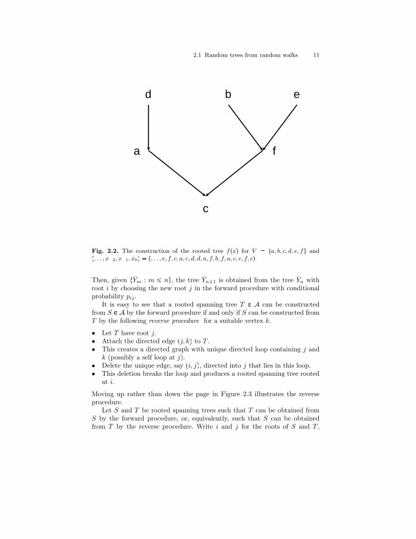
2.1 Random trees from random walks 11

d b e

a f

c

Fig. 2.2. The construction of the rooted tree fpxq for V ta, b, c, d, e, fu andp. . . , x2, x1, x0q p. . . , e, f, c, a, c, d, d, a, f, b, f, a, c, c, f, cq

Then, given tYm : m ¤ nu, the tree Yn1 is obtained from the tree Yn withroot i by choosing the new root j in the forward procedure with conditionalprobability pij .

It is easy to see that a rooted spanning tree T P A can be constructedfrom S P A by the forward procedure if and only if S can be constructed fromT by the following reverse procedure for a suitable vertex k.

• Let T have root j.• Attach the directed edge pj, kq to T .• This creates a directed graph with unique directed loop containing j and

k (possibly a self loop at j).• Delete the unique edge, say pi, jq, directed into j that lies in this loop.• This deletion breaks the loop and produces a rooted spanning tree rooted

at i.

Moving up rather than down the page in Figure 2.3 illustrates the reverseprocedure.

Let S and T be rooted spanning trees such that T can be obtained fromS by the forward procedure, or, equivalently, such that S can be obtainedfrom T by the reverse procedure. Write i and j for the roots of S and T ,

12 2 Around the continuum random tree

ij

k

ji

k

ji

k

Fig. 2.3. The forward procedure. The dashed line represents a directed path throughthe tree that may consist of several directed edges.

respectively, and write k for the (unique) vertex appearing in the descriptionof the reverse procedure. Denote by Q the transition matrix of the A-valuedprocess Y . We have observed that

• If S has root i and T has root j, then QST pij .• To get T from S we first attached the edge pi, jq and then deleted the

unique outgoing edge pj, kq from j.• To get S from T we would attach the edge pj, kq to T and then delete the

edge pi, jq.Thus, if we let ρ be the probability measure on A such that ρU is proportionalto the weight of U for U P A, then we have

ρSQST ρTRTS ,

where RTS : pjk. In particular,¸S

ρSQST ¸S

ρTRTS ρT ,

since R is a stochastic matrix. Hence ρ is the stationary distribution cor-responding to the irreducible transition matrix Q. That is, ρ is the one-

2.1 Random trees from random walks 13

dimensional marginal of the stationary chain Y . We also note in passing thatR is the transition matrix of the time-reversal of Y .

Thus,

πi ¸tρT : root of T is i u

°

TPAiweightpT q°

TPA weightpT q ,

as claimed. [\The proof we have given of Theorem 2.1 is from [21], where there is a

discussion of the history of the result.

2.1.2 Generating uniform random trees

Proposition 2.2. Let pXjqjPN0 be the natural random walk on the completegraph Kn with transition matrix P given by Pij : 1

n1 for i j and X0

uniformly distributed. Write

τν mintj ¥ 0 : Xj νu, ν 1, 2, . . . , n.

Let T be the directed subgraph of Kn with edges

pXτν, Xτν1q, ν X0.

Then T is uniformly distributed over the rooted spanning trees of Kn.

Proof. The argument in the proof of Theorem 2.1 plus the time-reversibilityof X. [\Remark 2.3. The set of rooted spanning trees of the complete graph Kn isjust the set of of nn1 rooted trees with vertices labeled by t1, 2, . . . , nu, andso the random tree T produced in Proposition 2.2 is nothing other than auniform rooted random tree with n labeled vertices.

Proposition 2.2 suggests a procedure for generating uniformly distributedrooted random trees with n labeled vertices. The most obvious thing to dowould be to run the chain X until all n states had appeared and then con-struct the tree T from the resulting sample path. The following algorithm,presented independently in [17, 35], improves on this naive approach by, ineffect, generating X0 and the pairs pXτν1, Xτν

q, ν X0 without generatingthe rest of the sample path of X.

Algorithm 2.4. Fix n ¥ 2. Let U2, . . . , Un be independent and uniformly dis-tributed on 1, . . . , n, and let Π be an independent uniform random permutationof 1, . . . , n.

14 2 Around the continuum random tree

5 4 6

2 3

1

Fig. 2.4. Step (i) of Algorithm 2.4 for n 6 and pV2, V3, V4, V5, V6q p1, 1, 3, 2, 3q

(i) For 2 ¤ i ¤ n connect vertex i to vertex Vi pi 1q ^ Ui (that is, build atree rooted at 1 with edges pi, Viq).

(ii)Relabel the vertices 1, . . . , n as Π1, . . . ,Πn to produce a tree rooted at Π1.

See Figure 2.4 for an example of Step (i) of the algorithm.

Proposition 2.5. The rooted random tree with n labeled vertices produced byAlgorithm 2.4 is uniformly distributed.

Proof. Let Z0, Z1, . . . be independent and uniform on 1, 2, . . . , n. Defineπ1, π2, . . . , πn, ξ1, ξ2, . . . , ξn P N0 and λ2, . . . , λn P t1, 2, . . . , nu by

ξ1 : 0,

π1 : Z0,

ξi1 : mintm ¡ ξi : Zm R tπ1, . . . , πiuu, 1 ¤ i ¤ n 1,

πi1 : Zξi1 , 1 ¤ i ¤ n 1,

λi1 : Zξi11, 1 ¤ i ¤ n 1.

Consider the random tree T labeled by t1, 2, . . . , nu with edges pπi, λiq, 2 ¤i ¤ n.

2.2 Random trees from conditioned branching processes 15

Note that this construction would give the same tree if the sequence Z wasreplaced by the subsequence Z 1 in which terms Zi identical with their prede-cessor Zi1 were deleted. The process Z 1 is just the natural random walk onthe complete graph. Thus, the construction coincides with the construction ofProposition 2.2. Hence, the tree T is a uniformly distributed tree on n labeledvertices. To complete the proof, we need only argue that this construction isequivalent to Algorithm 2.4.

It is clear that π is a uniform random permutation. The construction ofthe tree of T can be broken into two stages.

(i) Connect i to π1λi

, i 2, . . . , n.(ii) Relabel 1, . . . , n as π1, . . . , πn.

Thus, it will suffice to show that the conditional joint distribution of therandom variables π1

λi, i 2, . . . , n, given π is always the same as the (un-

conditional) joint distribution of the random variables Vi, i 2, . . . , n, inAlgorithm 2.4 no matter what the value of π is.

To see that this is so, first fix i and condition on Z1, . . . , Zξias well as π.

Note the following two facts.

• With probability 1 in we have ξi1 ξi 1, which implies that λi1 Zξi

and, hence, π1λi1

i.• Otherwise, ξi1 ξi M 1 for some random integer M ¥ 1. Con-

ditioning on the event tM mu, we have that the random variablesZξi1, . . . , Zξim are independent and uniformly distributed on the pre-viously visited states tπ1, . . . , πiu. In particular, λi1 Zξim is uni-formly distributed on tπ1, . . . , πiu, and so π1

λi1is uniformly distributed

on t1, . . . , iu.Combining these two facts, we see that

Ptπ1λi1

u |Z1, . . . , Zξi , πu 1n PtVi1 uu, 1 ¤ u ¤ i 1,

Ptπ1λi1

i |Z1, . . . , Zξiπu 1 pi 1qn PtVi1 iu,

as required. [\

2.2 Random trees from conditioned branching processes

If we were to ask most probabilists to propose a natural model for generatingrandom trees, they would first think of the family tree of a Galton–Watsonbranching process. Such a tree has a random number of vertices and if wefurther required that the random tree had a fixed number n of vertices, thenthey would suggest simply conditioning the total number of vertices in theGalton-Watson tree to be n. Interestingly, special cases of this mechanism forgenerating random trees produce trees that are also natural from a combina-torial perspective, as we shall soon see.

16 2 Around the continuum random tree

Let ppiqiPN0 be a probability distribution on the non-negative integers thathas mean one. Write T for the family tree of the Galton–Watson branchingprocess with offspring distribution ppiqiPN0 started with 1 individual in gen-eration 0. For n ¥ 1 denote by Tn a random tree that arises by conditioningon the total population size |T | being n (we suppose that the event t|T | nuhas positive probability). More precisely, we think of the trees T and Tn asrooted ordered trees: a rooted tree is ordered if we distinguish the offspring ofa vertex according with a “birth order”. Equivalently, a rooted ordered treeis a rooted planar tree: the birth order is given by the left-to-right orderingof offspring in the given embedding of the tree in the plane. The distributionof the random tree T is then

PtT tu ¹vPt

pdpv,tq

¹i¥0

pDiptqi

: ωptq,

where dpv, tq is the number of offspring of vertex v in t, and Diptq is thenumber of vertices in t with i offspring. Thus, PtTn tu is proportional toωptq.Example 2.6. If the offspring distribution ppiqiPN0 is the geometric distributionpi 2pi1q, i P N0, then Tn is uniformly distributed (on the set of rootedordered trees with n vertices).

Example 2.7. Suppose that the offspring distribution ppiqiPN0 is the Poissondistribution pi e1

i! , i P N0. If we randomly assign the labels t1, 2, . . . , nu tothe vertices of Tn and ignore the ordering, then Tn is a uniformly distributedrooted labeled tree with n vertices.

2.3 Finite trees and lattice paths

Although rooted planar trees are not particularly difficult to visualize, wewould like to have a quite concrete way of “representing” or “coordinatizing”the planar trees with n vertices that is amenable to investigating the behaviorof a random such trees as the number of vertices becomes large. The followingsimple observation is the key to the work of Aldous, Le Gall and many otherson the connections between the asymptotics of large random trees and modelsfor random paths.

Given a rooted planar tree with n vertices, start from the root and tra-verse the tree as follows. At each step move away from the root along theleftmost edge that has not been walked on yet. If this is not possible thenstep back along the edge leading toward the root. We obtain a with steps of

2.4 The Brownian continuum random tree 17

1 by plotting the height (that is, the distance from the root) at each step.Appending a 1 step at the beginning and a 1 step at the end gives a latticeexcursion path with 2n steps that we call the Harris path of the tree, althoughcombinatorialists usually call this object a Dyck path . We can reverse thisprocedure and obtain a rooted planar tree with n vertices from any latticeexcursion path with 2n steps.

Fig. 2.5. Harris path of a rooted combinatorial tree (figure courtesy of Jim Pitman).

2.4 The Brownian continuum random tree

Put Sn °ni1Xi, where the random variables Xi are independent with

PtXi 1u 12. Conditional on S1 1, the path S0, S1, . . . , SN , whereN mintk ¡ 0 : Sk 0u, is the Harris path of the Galton–Watson branchingprocess tree with offspring distribution pi 2pi1q, i P N0. Therefore, if wecondition on S1 1 and N 2n, we get the Harris path of the Galton–Watson branching process tree conditioned on total population size n, and wehave observed is the uniform rooted planar tree on n vertices.

We know that suitably re-scaled simple random walk converges to Brown-ian motion. Similarly, suitably re-scaled simple random walk conditioned tobe positive on the first step and return to zero for the first time at time 2nconverges as n Ñ 8 to the standard Brownian excursion. Of course, simplerandom walk is far from being the only process that has Brownian motion asa scaling limit, and so we might hope that there are other random trees withHarris paths that converge to standard Brownian excursion after re-scaling.The following result of Aldous [10] shows that this is certainly the case.

Theorem 2.8. Let Tn be a conditioned Galton–Watson tree, with offspringmean 1 and variance 0 σ2 8. Write Hnpkq, 0 ¤ k ¤ 2n for the Harrispath associated with Tn, and interpolate Hn linearly to get a continuous process

18 2 Around the continuum random tree

real-valued indexed by the interval r0, 2ns (which we continue to denote by Hn).Then, as n Ñ 8 through possible sizes of the unconditioned Galton–Watsontree,

σHnp2nuq?

n

0¤u¤1

ñ p2Bexu q0¤u¤1 ,

where Bex is the standard Brownian excursion and ñ is the usual weak con-vergence of probability measures on Cr0, 1s.

The Harris path construction gives a bijection between excursion-like lat-tice paths with steps of 1 and rooted planar trees. We will observe in Exam-ple 3.14 that any continuous excursion path gives rise to a tree-like object viaan analogy with one direction of this bijection. Hence Theorem 2.8 shows that,in some sense, any conditioned finite-variance Galton–Watson tree convergesafter re-scaling to the tree-like object associated with 2Bex. Aldous called thislatter object the Brownian continuum random tree .

2.5 Trees as subsets of `1

We have seen in Sections 2.3 and 2.4 that representing trees as continuouspaths allows us to use the metric structure on path space to make sense ofthe idea of a family of random trees converging to some limit random object.In this section we introduce an alternative “coordinatization” of tree-spaceas the collection of compact subsets of the Banach space `1 : tpx1, x2, . . .q :°

i |xi| 8u. This allows us to use the machinery that has been developed fordescribing random subsets of a metric space to give another way of expressingsuch convergence results.

Equip `1 with the usual norm. Any finite tree with edge lengths can beembedded isometrically as a subset of `1 (we think of such a tree as a one-dimensional cell complex, that is, as a metric space made up of the verticesof the tree and the connecting edges – not just as the finite metric spaceconsisting of the vertices themselves). For example, the tree of Figure 2.6 isisometric to the set

tte1 : 0 ¤ t ¤ dpρ, aquY tdpρ, dqe1 te2 : 0 ¤ t ¤ dpd, bquY tdpρ, dqe1 dpd, eqe2 te3 : 0 ¤ t ¤ dpe, cqu,

where e1 p1, 0, 0, . . .q, e2 p0, 1, 0, . . .q, etc.Recall Algorithm 2.4 for producing a uniform tree on n labeled vertices.

Let Sn be the subset of `1 that corresponds to the tree produced by thealgorithm. We think of this tree as having edge lengths all equal to 1. Moreprecisely, define a random length random sequence pCn

j , Bnj q, 0 ¤ j ¤ Jn, as

follows:

• Cn0 Bn

0 : 0,

2.5 Trees as subsets of `1 19

a

c

bde

r

Fig. 2.6. A rooted tree with edge lengths

• Cnj is the jth element of ti : Ui i 1u,

• Bnj : UCn

j.

Define ρn : r0, CnJns Ñ `1 by ρnp0q : 0 and

ρnpxq : ρnpBnj q px Cn

j qej1 for Cnj x ¤ Cn

j1, 0 ¤ j ¤ Jn 1.

Put Sn : ρnpr0, CnJnsq.

It is not hard to show that

ppn12Cn1 , n

12Bn1 q, pn12Cn

2 , n12Bn

2 q, . . .qñ ppC1, B1q, pC2, B2q, . . .q,

where ñ denotes weak convergence and ppC1, B1q, pC2, B2q, . . .q are definedas follows. Put C0 B0 : 0. Let pC1, C2, . . .q be the arrival times in aninhomogeneous Poisson process on R with intensity t dt. Let Bj : ξjCj ,where the tξjujPN are independent, identically distributed uniform randomvariables on r0, 1s, independent of tCjujPN.

Define ρ : R Ñ `1 by ρp0q : 0 and

ρpxq : ρpBjq px Cjqej1 for Cj x ¤ Cj1.

20 2 Around the continuum random tree

SetS :

¤t¥0

ρpr0, tsq.

It seems reasonable thatn12Sn ñ S

in some sense. Aldous [12] showed that S is almost surely a compact subset of`1 and that there is convergence in the sense of weak convergence of randomcompact subsets of `1 equipped with the Hausdorff metric that we will discussin Section 4.1. Aldous studied S further in [13, 10]. In particular, he showedthat S is tree-like in various senses: for example, for any two points x, y P Sthere is a unique path connecting x and y (that is, a unique homeomorphicimage of the unit interval), and this path has length x y1.

Because the uniform rooted tree with n labeled vertices is a conditionedGalton–Watson branching process (for the Poisson offspring distribution), wesee from Theorem 2.8 that the Poisson line-breaking “tree” S is essentially thesame as the Brownian continuum random tree, that is, the random tree-likeobject associated with the random excursion path 2Bex. In fact, the randomtree ρpCnq has the same distribution as the subtree of the Brownian CRTspanned by n i.i.d. uniform points on the unit interval.

3

R-trees and 0-hyperbolic spaces

3.1 Geodesic and geodesically linear metric spaces

We follow closely the development in [39] in this section and leave some of themore straightforward proofs to the reader.

Definition 3.1. A segment in a metric space pX, dq is the image of an isom-etry α : ra, bs Ñ X. The end points of the segment are αpaq and αpbq.Definition 3.2. A metric space pX, dq is geodesic if for all x, y P X, thereis a segment in X with endpoints tx, yu, and pX, dq is geodesically linear if,for all x, y P X, there is a unique segment in X with endpoints tx, yu.Example 3.3. Euclidean space Rd is geodesically linear. The closed annulustz P R2 : 1 ¤ |z| ¤ 2u is not geodesic in the metric inherited from R2, butit is geodesic in the metric defined by taking the infimum of the Euclideanlengths of piecewise-linear paths between two points. The closed annulus isnot geodesically linear in this latter metric: for example, a pair of points ofthe form z and z are the endpoints of two segments – see Figure 3.1. Theopen annulus tz P R2 : 1 |z| 2u is not geodesic in the metric definedby taking the infimum over all piecewise-linear paths between two points: forexample, there is no segment that has a pair of points of the form z and zas its endpoints.

Lemma 3.4. Consider a metric space pX, dq. Let σ be a segment in X withendpoints x and z, and let τ be a segment in X with endpoints y and z.

(a) Suppose that dpu, vq dpu, zq dpz, vq for all u P σ and v P τ . Then σY τis a segment with endpoints x and y.

(b) Suppose that σXτ tzu and σYτ is a segment. Then σYτ has endpointsx and y.

22 3 R-trees and 0-hyperbolic spaces

z-z

Fig. 3.1. Two geodesics with the same endpoints in the intrinsic path length metricon the annulus

Lemma 3.5. Let pX, dq be a geodesic metric space such that if two segmentsof pX, dq intersect in a single point, which is an endpoint of both, then theirunion is a segment. Then pX, dq is a geodesically linear metric space.

Proof. Let σ, τ be segments, both with endpoints u, v. Fix w P σ, and define w1

to be the point of τ such that dpu,wq dpu,w1q (so that dpv, wq dpv, w1q).We have to show w w1.

Let ρ be a segment with endpoints w,w1. Now σ σ1 Y σ2, where σ1 is asegment with endpoints u,w, and σ2 is a segment with endpoints w, v – seeFigure 3.2.

We claim that either σ1 X ρ twu or σ2 X ρ twu. This is so becauseif x P σ1 X ρ and y P σ2 X ρ, then dpx, yq dpx,wq dpw, yq, and eitherdpw, yq dpw, xq dpx, yq or dpw, xq dpw, yq dpx, yq, depending on howx, y are situated in the segment ρ. It follows that either x w or y w,establishing the claim.

Now, if σ1 X ρ twu, then, by assumption, σ1 Y ρ is a segment, and byLemma 3.4(b) its endpoints are u,w1. Since w P σ1 Y ρ, dpu,w1q dpu,wq dpw,w1q, so w w1. Similarly, if σ2 X ρ twu then w w1. [\Lemma 3.6. Consider a geodesically linear metric space pX, dq.

3.2 0-hyperbolic spaces 23

t

w’

u v

w

r

s1 s2

s

Fig. 3.2. Construction in the proof of Lemma 3.5

(i) Given points x, y, z P X, write σ for the segment with endpoints x, y.Then z P σ if and only if dpx, yq dpx, zq dpz, yq.

(ii) The intersection of two segments in X is also a segment if it is non-empty.

(iii) Given x, y P X, there is a unique isometry α : r0, dpx, yqs Ñ X such thatαp0q x and αpdpx, yqq y. Write rx, ys for the resulting segment. Ifu, v P rx, ys, then ru, vs rx, ys.

3.2 0-hyperbolic spaces

Definition 3.7. For x, y, v in a metric space pX, dq, set

px yqv : 12pdpx, vq dpy, vq dpx, yqq

– see Figure 3.3.

Remark 3.8. For x, y, v, t P X,

0 ¤ px yqv ¤ dpx, vq ^ dpy, vq

24 3 R-trees and 0-hyperbolic spaces

xy

w

v

Fig. 3.3. px yqv dpw, vq in this tree

andpx yqt dpt, vq px yqv px tqv py tqt.

Definition 3.9. A metric space pX, dq is 0-hyperbolic with respect to v if forall x, y, z P X

px yqv ¥ px zqv ^ py zqv– see Figure 3.4.

Lemma 3.10. If the metric space pX, dq is 0-hyperbolic with respect to somepoint of X, then pX, dq is 0-hyperbolic with respect to all points of X.

Remark 3.11. In light of Lemma 3.10, we will refer to a metric space that is0-hyperbolic with respect to one, and hence all, of its points as simply being0-hyperbolic. Note that any subspace of a 0-hyperbolic metric space is also0-hyperbolic.

Lemma 3.12. The metric space pX, dq is 0-hyperbolic if and only if

dpx, yq dpz, tq ¤ maxtdpx, zq dpy, tq, dpy, zq dpx, tqufor all x, y, z, t P X,

3.2 0-hyperbolic spaces 25

x

z

y

v

Fig. 3.4. The 0-hyperbolicity condition holds for this tree. Here px yqv and py zqvare both given by the length of the dotted segment, and px zqv is the length of thedashed segment. Note that px yqv ¥ px zqv ^py zqv, with similar inequalities whenx, y, z are permuted.

Remark 3.13. The set of inequalities in Lemma 3.12 is usually called the four-point condition – see Figure 3.5.

Example 3.14. Write CpRq for the space of continuous functions from Rinto R. For e P CpRq, put ζpeq : inftt ¡ 0 : eptq 0u and write

U :$&%e P CpRq :

ep0q 0, ζpeq 8,eptq ¡ 0 for 0 t ζpeq,and eptq 0 for t ¥ ζpeq

,.-for the space of positive excursion paths. Set U ` : te P U : ζpeq `u.

We associate each e P U ` with a compact metric space as follows. Definean equivalence relation e on r0, `s by letting

u1 e u2, iff epu1q infuPru1^u2,u1_u2s

epuq epu2q.

Consider the following semi-metric on r0, `s

26 3 R-trees and 0-hyperbolic spaces

x

y

z

t

Fig. 3.5. The four-point condition holds on a tree: dpx, zq dpy, tq ¤ dpx, yq dpz, tq dpx, tq dpy, zq

dTepu1, u2q : epu1q 2 infuPru1^u2,u1_u2s

epuq epu2q,

that becomes a true metric on the quotient space Te : r0, `se– see Fig-

ure 3.6.It is straightforward to check that the quotient map from r0, `s onto Te is

continuous with respect to dTe. Thus, pTe, dTe

q is path-connected and compactas the continuous image of a metric space with these properties. In particular,pTe, dTeq is complete. It is not difficult to check that pTe, dTeq satisfies thefour-point condition, and, hence, is 0-hyperbolic.

3.3 R-trees

3.3.1 Definition, examples, and elementary properties

Definition 3.15. An R-tree is a metric space pX, dq with the following prop-erties.

Axiom (a) The space pX, dq is geodesic.

3.3 R-trees 27

0 a b 1

Fig. 3.6. An excursion path on r0, 1s determines a distance between the points aand b

Axiom (b) If two segments of pX, dq intersect in a single point, which is anendpoint of both, then their union is a segment.

Example 3.16. Finite trees with edge lengths (sometimes called weightedtrees) are examples of R-trees. To be a little more precise, we don’t thinkof such a tree as just being its finite set of vertices with a collection of dis-tances between them, but regard the edges connecting the vertices as alsobeing part of the metric space.

Example 3.17. Take X to be the plane R2 equipped with the metric

dppx1, x2q, py1, y2qq :#|x2 y2|, if x1 y1,

|x1 y1| |x2| |y2|, if x1 y1.

That is, we think of the plane as being something like the skeleton of afish, in which the horizontal axis is the spine and vertical lines are the ribs.In order to compute the distance between two points on different ribs, we usethe length of the path that goes from the first point to the spine, then alongthe spine to the rib containing the second point, and then along that secondrib – see Figure 3.7.

28 3 R-trees and 0-hyperbolic spaces

Fig. 3.7. The distance between two points of R2 in the metric of Example 3.17 isthe (Euclidean) length of the dashed path

Example 3.18. Consider the collection T of bounded subsets of R that containtheir supremum. We can think of the elements of T as being arrayed in atree–like structure in the following way. Using genealogical terminology, writehpBq : supB for the real–valued generation to which B P T belongs andB|t : pBXs8, tsqYttu P T for t ¤ hpBq for the ancestor of B in generationt. For A,B P T the generation of the most recent common ancestor of A andB is τpA,Bq : suptt ¤ hpAq ^ hpBq : A|t B|tu. That is, τpA,Bq isthe generation at which the lineages of A and B diverge. There is a naturalgenealogical distance on T given by

DpA,Bq : rhpAq τpA,Bqs rhpBq τpA,Bqs.See Figure 3.8.

It is not difficult to show that the metric space pT , Dq is a R-tree. Forexample, the segment with end-points A and B is the set tA|t : τpA,Bq ¤t ¤ hpAqu Y tB|t : τpA,Bq ¤ t ¤ hpBqu.

The metric space pT , Dq is essentially “the” real tree of [47, 137] (thelatter space has as its points the bounded subsets of R that contain theirinfimum and the corresponding metric is such that the map from pT , Dq intothis latter space given by A ÞÑ A is an isometry). With a slight abuse of

3.3 R-trees 29

A

B

Cu t s

Fig. 3.8. The set C is the most recent common ancestor of the sets A, B R

thought of as points of “the” real tree of Example 3.18. The distance DpA, Bq isrs us rt us.

nomenclature, we will refer here to pT , Dq as the real tree. Note that pT , Dqis huge: for example, the removal of any point shatters T into uncountablymany connected components.

Example 3.19. We will see in Example 3.37 that the compact 0-hyperbolicmetric space pTe, dTe

q of Example 3.14 that arises from an excursion pathe P U is a R-tree.

The following result is a consequence of Axioms (a) and (b) and Lemma 3.5.

Lemma 3.20. An R-tree is geodesically linear. Moreover, if pX, dq is a R-treeand x, y, z P X then rx, ys X rx, zs rx,ws for some unique w P X.

Remark 3.21. It follows from Lemma 3.4, Lemma 3.6 and Lemma 3.20 thatAxioms (a) and (b) together imply following condition that is stronger thanAxiom (b):

Axiom (b’) If pX, dq is a R-tree, x, y, z P X and rx, ys X rx, zs txu, thenrx, ys Y rx, zs ry, zs

30 3 R-trees and 0-hyperbolic spaces

Lemma 3.22. Let x, y, z be points of a R-tree pX, dq, and write w for theunique point such that rx, ys X rx, zs rx,ws.(i) The points x, y, z, w and the segments connecting them form a Y shape,

with x, y, z at the tips of the Y and w at the center. More precisely,ry, ws X rw, zs twu, ry, zs ry, ws Y rw, zs and rx, ys X rw, zs twu.

(ii) If y1 P rx, ys and z1 P rx, zs, then

dpy1, z1q #

|dpx, y1q dpx, z1q|, if dpx, y1q ^ dpx, z1q ¤ dpx,wq,dpx, y1q dpx, z1q 2dpx,wq, otherwise.

(iii) The “centroid” w depends only on the set tx, y, zu, not on the order inwhich the elements are written.

Proof. (i) Since y, w P rx, ys, we have ry, ws rx, ys. Similarly, rw, zs rx, zs.So, if u P ry, ws X rw, zs, then u P rx, ys X rx, zs rx,ws. Hence u P rx,ws Xry, ws twu (because w P rx, ys). Thus, ry, ws X rw, zs twu, and ry, zs ry, ws Y rw, zs by Axiom (b’).

Now, since w P rx, ys, we have rx, ys rx,ws Y rw, ys, so rx, ys X rw, zs prx,ws X rw, zsq Y pry, ws X rw, zsq, and both intersections are equal to twu(w P rx, zs).(ii) If dpx, y1q ¤ dpx,wq then y1, z1 P rx, zs, and so dpy1, z1q |dpx, y1qdpx, z1q|.Similarly, if dpx, z1q ¤ dpx,wq, then y1, z1 P rx, ys, and once again dpy1, z1q |dpx, y1q dpx, z1q|.

If dpx, y1q ¡ dpx,wq and dpx, z1q ¡ dpx,wq, then y1 P ry, ws and z1 P rz, ws.Hence, by part (i),

dpy1, z1q dpy1, wq dpw, z1q pdpx, y1q dpx,wqq pdpx, z1q dpx,wq dpx, y1q dpx, z1q 2dpx,wq.

(iii) We have by part (i) that

ry, xs X ry, zs ry, xs X pry, ws Y rw, zsq ry, ws Y pry, xs X rw, zsq ry, ws Y pry, ws X rw, zsq Y prw, xs X rw, zsq

Now ry, ws X rw, zs twu by part (1) and rw, xs X rw, zs twu sincew P rx, zs. Hence, ry, xs X ry, zs ry, ws. Similarly, rz, xs X rz, ys rz, ws, andpart (iii) follows. [\Definition 3.23. In the notation of Lemma 3.22, write Y px, y, zq : w forthe centroid of tx, y, zu.Remark 3.24. Note that we have

rx, ys X rw, zs rx, zs X rw, ys ry, zs X rw, xs twu.Also, dpx,wq py zqx, dpy, wq px zqy, and dpz, wq px yqz. In Figure 3.3,Y px, y, vq w.

3.3 R-trees 31

Corollary 3.25. Consider a R-tree pX, dq and points x0, x1, . . . , xn P X. Thesegment rx0, xns is a subset of

ni1rxi1, xis.

Proof. If n 2, then, by Lemma 3.22,

rx0, x2s rx0, Y px0, x1, x2qs Y rY px0, x1, x2q, x2s rx0, x1s Y rx1, x2s.If n ¡ 2, then rx0, xns rx0, xn1s Y rxn1, xns by the case n 2, and theresult follows by induction on n. [\Lemma 3.26. Consider a R-tree pX, dq. Let α : ra, bs Ñ X be a continuousmap. If x αpaq and y αpbq, then rx, ys is a subset of the image of α.

Proof. Let A denote the image of α. Since A is a closed subset of X (beingcompact as the image of a compact interval by a continuous map), it is enoughto show that every point of rx, ys is within distance ε of A, for all ε ¡ 0.

Given ε ¡ 0, the collection tα1pBpx, ε2qq : x P Au is an open coveringof the compact metric space ra, bs, so there is a number δ ¡ 0 such that anytwo points of ra, bs that are distance less than δ apart belong to some commonset in the cover.

Choose a partition of ra, bs, say a t0 tn b, so that for 1 ¤ i ¤ nwe have ti ti1 δ, and, therefore, dpαpti1q, αptiqq ε. Then all pointsof rαpti1q, αptiqs are at distance less than ε from tαpti1q, αptiqu A for1 ¤ i ¤ n. Finally, rx, ys n

i1rαpti1q, αptiqs, by Corollary 3.25. [\Definition 3.27. For points x0, x1, . . . , xn in a R-tree pX, dq, write rx0, xns rx0, x1, . . . , xns to mean that, if α : r0, dpx0, xnqs Ñ X is the unique isom-etry with αp0q x0 and αpdpx0, xnqq xn, then xi αpaiq, for somea0, a1, a2, . . . , an with 0 a0 ¤ a1 ¤ a2 ¤ ¤ an dpx0, xnq.Lemma 3.28. Consider a R-tree pX, dq. If x0, . . . , xn P X, xi xi1 for1 ¤ i ¤ n 2 and rxi1, xis X rxi, xi1s txiu for 1 ¤ i ¤ n 1, thenrx0, xns rx0, x1, . . . , xns.Proof. There is nothing to prove if n ¤ 2. Suppose n 3. We can assumex0 x1 and x2 x3, otherwise there is again nothing to prove. Let w Y px0, x2, x3q.

Now w P rx0, x2s and x1 P rx0, x2s, so rx2, ws X rx2, x1s rx2, vs, where vis either w or x1, depending on which is closer to x2. But rx2, ws X rx2, x1s rx2, x3s X rx2, x1s tx2u, so v x2.

Since x1 x2, we conclude that w x2. Hence rx0, x2s X rx2, x3s tx2u,which implies rx0, x3s rx0, x2, x3s rx0, x1, x2, x3s.

Now suppose n ¡ 3. By induction,

rx0, xn1s rx0, x1, . . . , xn2, xn1s rx0, xn2, xn1s.By the n 3 case,

rx0, xns rx0, xn2, xn1, xns rx0, x1, . . . , xn2, xn1, xnsas required. [\

32 3 R-trees and 0-hyperbolic spaces

3.3.2 R-trees are 0-hyperbolic

Lemma 3.29. A R-tree pX, dq is 0-hyperbolic.

Proof. Fix v P X. We have to show

px yqv ¥ px zqv ^ py zqvpx zqv ¥ px yqv ^ py zqvpy zqv ¥ px yqv ^ px zqv

for all x, y, z. Note that if this is so, then one of px yqv, px zqv, py zqv is atleast as great as the other two, which are equal.

Let q Y px, v, yq, r Y py, v, zq, and s Y pz, v, xq. We have px yqv dpv, qq, py zqv dpv, sq, and pz xqv dpv, rq. We may assume without lossof generality that

dpv, qq ¤ dpv, rq ¤ dpv, sq,in which case have to show that q r – see Figure 3.9.

v

sx y

q=r

z

Fig. 3.9. The configuration demonstrated in the proof of Lemma 3.29

Now r, s P rv, zs by definition, and dpv, rq ¤ dpv, sq, so that rv, ss rv, r, ss.Also, by definition of s, rv, xs rv, s, xs rv, r, s, xs. Hence r P rv, xsXrv, ys rv, qs. Since dpv, qq ¤ dpv, rq, we have q r, as required. [\

3.3 R-trees 33

Remark 3.30. Because any subspace of a 0-hyperbolic space is still 0-hyperbolic, we can’t expect that the converse to Lemma 3.29 holds. However,we will see in Theorem 3.38 that any 0-hyperbolic space is isometric to asubspace of a R-tree.

3.3.3 Centroids in a 0-hyperbolic space

Definition 3.31. A set ta, b, cu R is called an isosceles triple if

a ¥ b^ c, b ¥ c^ a, and c ¥ a^ b.

(This means that at least two of a, b, c are equal, and not greater than thethird.)

Remark 3.32. The metric space pX, dq is 0-hyperbolic if and only if px yqv, px zqv, py zqv is an isosceles triple for all x, y, z, v P X.

Lemma 3.33. (i) If ta, b, cu is any triple then

ta^ b, b^ c, c^ auis an isosceles triple.(ii) If ta, b, cu and td, e, fu are isosceles triples then so is

ta^ d, b^ e, c^ fu.Lemma 3.34. Consider a 0-hyperbolic metric space pX, dq. Let σ, τ be seg-ments in X with endpoints v, x and v, y respectively. Write x y : px yqv.(i) If x1 P σ, then x1 P τ if and only if dpv, x1q ¤ x y.(ii)If w is the point of σ at distance x y from v, then σX τ is a segment with

endpoints v and w.

Proof. If dpx1, vq ¡ dpy, vq then x1 R τ , and dpx1, vq ¡ x y, so we can assumethat dpx1, vq dpy, vq. Let y1 be the point in τ such that dpv, x1q dpv, y1q.Define

α x y, β x1 y, γ x x1, α1 x1 y1.Since x1 P σ and y1 P τ , we have γ dpv, x1q dpv, y1q y y1. Hence,

pα, β, γq and pα1, β, γq are isosceles triples. We have to show that x1 P τ if andonly if α ¥ γ. The two cases α γ and α ¥ γ are illustrated in Figure 3.10and Figure 3.11 respectively.

Now,β x1 y ¤ dpv, x1q x x1 γ.

Also,

α1 dpv, x1q 12dpx1, y1q γ 1

2dpx1, y1q ¤ γ

and

34 3 R-trees and 0-hyperbolic spaces

xy

x’ y’

v

Fig. 3.10. First case of the construction in the proof of Lemma 3.34. Here γ iseither of the two equal dashed lengths and α β α1 is the dotted length. Asclaimed, α γ and x1Rτ .

x1 P τ ô x1 y1 ô dpx1, y1q 0 ô α1 γ.

Moreover, α1 γ if and only if β γ, because pα1, β, γq is an isoscelestriple and α1, β ¤ γ. Since pα, β, γq is also an isosceles triple, the equalityβ γ is equivalent to the inequality α ¥ γ. This proves part (i). Part (ii) ofthe lemma follows immediately. [\Lemma 3.35. Consider a 0-hyperbolic metric space pX, dq. Let σ, τ be seg-ments in X with endpoints v, x and v, y respectively. Set x y : px yqv.Write w for the point of σ at distance x y from v (so that w is an endpointof σ X τ by Lemma 3.34). Consider two points x1 P σ, y1 P τ , and supposedpx1, vq ¥ x y and dpy1, vq ¥ x y. Then

dpx1, y1q dpx1, wq dpy1, wq.Proof. The conclusion is clear if dpx1, vq xy (when x1 w) or dpy1, vq xy(when y1 w), so we assume that dpx1, vq ¡ x y and dpy1, vq ¡ x y. As inthe proof of Lemma 3.34, we put

α x y, β x1 y, γ x x1, α1 x1 y1,

3.3 R-trees 35

xy

x’= y’

v

Fig. 3.11. Second case of the construction in the proof of Lemma 3.34. Here γ β α1 is the dashed length and α is the dotted length. As claimed, α ¥ γ andx1 P τ .

and we also put γ1 y y1, so that γ dpv, x1q and γ1 dpv, y1q. Thus, α γ.Hence, α β since pα, β, γq is an isosceles triple. Also, α γ1, so that β γ1.Hence, α α1 β because pα1, β, γq is an isosceles triple.

By definition of α1,

dpx1, y1q dpv, x1q dpv, y1q 2α1

dpv, x1q dpv, y1q 2α.

Since w P σ X τ , α dpv, wq dpv, x1q, dpv, y1q and σ, τ are segments, itfollows that

dpx1, wq dpv, x1q α

anddpy1, wq dpv, y1q α,

and the lemma follows on adding these equations. [\

36 3 R-trees and 0-hyperbolic spaces

3.3.4 An alternative characterization of R-trees

Lemma 3.36. Consider a 0-hyperbolic metric space pX, dq. Suppose that thereis a point v P X such that for every x P X there is a segment with endpointsv, x. Then pX, dq is a R-tree.

Proof. Take x, y P X and let σ, τ be segments with endpoints v, x and v, yrespectively.

By Lemma 3.34, if w is the point of σX τ at distance px yqv from v, thenσ is the union pσ X τq Y σ1, where

σ1 : tu P σ : dpv, uq ¥ px yqvu

is a segment with endpoints w, x. Similarly, τ is the union pσX τqY τ1, where

τ1 : tu P τ : dpv, uq ¥ px yqvu

is a segment with endpoints w, y.By Lemma 3.35 and Lemma 3.4, σ1Y τ1 is a segment with endpoints x, y.

Thus, pX, dq is geodesic.Note that by Lemma 3.34, σ X τ is a segment with endpoints v, w. Also,

by Lemma 3.34, if σ X τ twu then px yqv 0 and σ1 σ, τ1 τ . Hence,σ Y τ is a segment. Now, by Lemma 3.10, we may replace v in this argumentby any other point of X. Hence, pX, dq satisfies the axioms for a R-tree. [\Example 3.37. We noted in Example 3.14 that the compact metric spacepTe, dTe

q that arises from an excursion path e P U is 0-hyperbolic. We canuse Lemma 3.36 to show that pTe, dTe

q is a R-tree. Suppose that e P U `. Takex P Te and write t for a point in r0, `s such that x is the image of t underthe quotient map from r0, `s onto Te. Write v P Te for the image of 0 P r0, `sunder the quotient map from r0, `s onto Te. Note that v is also the image of` P r0, `s. For h P r0, eptqs, set λh : supts P r0, ts : epsq hu. Then the imageof the set tλh : h P r0, eptqsu r0, `s under the quotient map is a segment inTe that has endpoints v and x.

3.3.5 Embedding 0-hyperbolic spaces in R-trees

Theorem 3.38. Let pX, dq be a 0-hyperbolic metric space. There exists a R-tree pX 1, d1q and an isometry φ : X Ñ X 1.

Proof. Fix v P X. Write x y : px yqv for x, y P X. Let

Y tpx,mq : x P X,m P R and 0 ¤ m ¤ dpv, xqu.

Define, for px,mq, py, nq P Y ,

px,mq py, nq if and only if x y ¥ m n.

3.3 R-trees 37

This is an equivalence relation on Y . Let X 1 Y , and let xx,my denotethe equivalence class of px,mq. We define the metric by

d1pxx,my, xy, nyq m n 2rm^ n^ px yqs.

The construction is illustrated in Figure 3.12.

y x

(x,m) ~ (y,m)m

V

Fig. 3.12. The embedding of Theorem 3.38. Solid lines represent points that are inX, while dashed lines represent points that are added to form X 1.

It follows by assumption that d1 is well defined. Note that

d1pxx,my, xx, nyq |m n|

and xx, 0y xv, 0y for all x P X, so d1pxx,my, xv, 0yq m. Clearly d1 issymmetric, and it is easy to see that d1pxx,my, xy, nyq 0 if and only ifxx,my xy, ny. Also, in X 1,

pxx,my xy, nyqxv,0y m^ n^ px yq.

If xx,my, xy, ny and xz, py are three points of X 1, then

tm^ n, n^ p, p^mu

38 3 R-trees and 0-hyperbolic spaces

is an isosceles triple by Lemma 3.33(1). Hence, by Lemma 3.33(2), so is tm^n^px yq, n^p^py zq, p^m^pz xqu. It follows that pX 1, d1q is a 0-hyperbolicmetric space.

If xx,my P X 1, then the mapping α : r0,ms Ñ X 1 given by αpnq xx, ny isan isometry, so the image of α is a segment with endpoints xv, 0y and xx,my. Itnow follows from Lemma 3.36 that pX 1, d1q is a R-tree. Further, the mappingφ : X Ñ X 1 defined by φpxq xx, dpv, xqy is easily seen to be an isometry. [\

3.3.6 Yet another characterization of R-trees

Lemma 3.39. Let pX, dq be a R-tree. Fix v P X.

(i) For x, y P Xztvu, rv, xs X rv, ys tvu if and only if x, y are in the samepath component of Xztvu.

(ii)The space Xztvu is locally path connected, the components of Xztvu coin-cide with its path components, and they are open sets in X.

Proof. (i) Suppose that rv, xsXrv, ys tvu. It can’t be that v P rx, ys, becausethat would imply rx, vs X rv, ys tvu. Thus, rx, ys Xztvu and x, y are inthe same path component of Xztvu. Conversely, if α : ra, bs Ñ Xztvu is acontinuous map, with x αpaq, y αpbq, then ra, bs is a subset of the imageof α by Lemma 3.26, so v R rx, ys, and rv, xs X rv, ys tvu by Axiom (b’) fora R-tree.(ii) For x P Xztvu, the set U : ty P X : dpx, yq dpx, vqu is an open setin X, U Xztvu, x P U , and U is path connected. For if y, z P U , thenrx, ysY rx, zs U , and so ry, zs U by Corollary 3.25. Thus, Xztvu is locallypath connected. It follows that the path components of Xztvu are both openand closed, and (ii) follows easily. [\Theorem 3.40. A metric space pX, dq is a R-tree if and only if it is connectedand 0-hyperbolic.

Proof. An R-tree is geodesic, so it is path connected. Hence, it is connected.Therefore, it is 0-hyperbolic by Lemma 3.29.

Conversely, assume that a metric space pX, dq is connected and 0-hyperbolic. By Theorem 3.38 there is an embedding of pX, dq in a R-treepX 1, d1q. Let x, y P X, suppose v P X 1zX and v P rx, ys. Then rv, xs X rv, ys tvu and so by Lemma 3.39, x, y are in different components of Xztvu.

Let C be the component of Xztvu containing x. By Lemma 3.39, C is openand closed, so XXC is open and closed in X. Since x P XXC, y R XXC, thiscontradicts the connectedness of X. Thus, rx, ys X and pX, dq is geodesic.It follows that pX, dq is a R-tree by Lemma 3.36. [\Example 3.41. Let P denote the collection of partitions of the positive integersN. There is a natural partial order ¤ on P defined by P ¤ Q if every blockof Q is a subset of some block of P (that is, the blocks of P are unions of

3.4 R–trees without leaves 39

blocks of Q). Thus, the partition tt1u, t2u, . . .u consisting of singletons is theunique largest element of P, while the partition tt1, 2, . . .uu consisting of asingle block is the unique smallest element. Consider a function Π : R ÞÑ Pthat is non-increasing in this partial order. Suppose that Πp0q tt1u, t2u, . . .uand Πptq tt1, 2, . . .uu for all t sufficiently large. Suppose also that if Π isright-continuous in the sense that if i and j don’t belong to the same block ofΠptq for some t P R, then they don’t belong to the same block of Πpuq foru ¡ t sufficiently close to t.

Let T denote the set consisting of points of the form pt, Bq, where t P Rand B P Πptq. Given two point ps,Aq, pt, Bq P T , set

mpps,Aq, pt, Bqq: inftu ¡ s^ t : A and B subsets of a common block of Πpuqu,

and put

dpps,Aq, pt, Bqq : rmpps,Aq, pt, Bqq ss rmpps,Aq, pt, Bqq ts.It is not difficult to check that d is a metric that satisfies the four pointcondition and that the space T is connected. Hence, pT, dq is a R-tree byTheorem 3.40. The analogue of this construction with N replaced by t1, 2, 3, 4uis shown in Figure 3.13.

Moreover, if we let T denote the completion of T with respect to the metricd, then T is also a R-tree. It is straightforward to check that T is compact ifand only if Πptq has finitely many blocks for all t ¡ 0.

Write δ for the restriction of d to the positive integers N, so that

δpi, jq 2 inftt ¡ 0 : i and j belong to the same block of Πptqu.The completion S of N with respect to δ is isometric to the closure of N in T ,and S is compact if and only if Πptq has finitely many blocks for all t ¡ 0. Notethat δ is an ultrametric , that is, δpx, yq ¤ δpx, zq_ δpz, yq for x, y, z P S. Thisimplies that at least two of the distances are equal and are no smaller thanthe third. Hence, all triangles are isosceles. When S is compact, the open ballsfor the metric δ coincide with the closed balls and are obtained by taking theclosure of the blocks of Πptq for t ¡ 0. In particular, S is totally disconnected.

The correspondence between coalescing partitions, tree structures and ul-trametrics is a familiar idea in the physics literature – see, for example, [109].

3.4 R–trees without leaves

3.4.1 Ends

Definition 3.42. An R-tree without leaves is a R–trees pT, dq that satisfiesthe following extra axioms.

40 3 R-trees and 0-hyperbolic spaces

4

3

2

1

1,2,3,4 1,2,3,4 1,2,3,4 1,2,3,4

Fig. 3.13. The construction of a R-tree from a non-increasing function taking valuesin the partitions of t1, 2, 3, 4u.

Axiom (c) The metric space pT, dq is complete.Axiom (d) For each x P T there is at least one isometric embedding θ : R Ñ T

with x P θpRq.Example 3.43. “The” real tree pT , Dq of Example 3.18 satisfies Axioms (c)and (d).

We will suppose in this section that we are always working with a R-treepT, dq that is without leaves.

Definition 3.44. An end of T is an equivalence class of isometric embeddingsfrom R into T , where we regard two such embeddings φ and ψ as beingequivalent if there exist α P R and β P R such that α β ¥ 0 and φptq ψpt αq for all t ¥ β. Write E for the set of ends of T .

By Axiom (d), E has at least 2 points. Fix a distinguished element : of E.For each x P T there is a unique isometric embedding κx : R Ñ T such thatκxp0q x and κx is a representative of the equivalence class of :. Similarly,for each ξ P E : Ezt:u there is at least one isometric embedding θ : R Ñ Tsuch that t ÞÑ θptq, t ¥ 0, is a representative of the equivalence class of ξ

3.4 R–trees without leaves 41

and t ÞÑ θptq, t ¥ 0, is a representative of the equivalence class of :. Denotethe collection of all such embeddings by Θξ. If θ, θ1 P Θξ, then there existsγ P R such that θptq θ1pt γq for all t P R. Thus, it is possible to select anembedding θξ P Θξ for each ξ P E in such a way that for any pair ξ, ζ P Ethere exists t0 (depending on ξ, ζ) such that θξptq θζptq for all t ¤ t0 (andθξpst0,8rq X θζpst0,8rq H). Extend θξ to R : R Y t8u by settingθξp8q : : and θξp8q : ξ.

Example 3.45. The ends of the real tree pT , Dq of Example 3.18 can beidentified with the collection consisting of the empty set and the elementsof E, where E consists of subsets B R such that 8 inf B andsupB 8. If we choose : to be the empty set so that E plays therole of E, then we can define the isometric embedding θA for A P E byθAptq : pAXs 8, tsq Y ttu A|t, in the notation of Example 3.18.

The map pt, ξq ÞÑ θξptq from RE (resp. RE) into T (resp. T YE)is surjective. Moreover, if η P T Y E is in θξpRq X θζpRq for ξ, ζ P E,then θ1

ξ pηq θ1ζ pηq. Denote this common value by hpηq, the height of η.

In genealogical terminology, we think of hpηq as the generation to which ηbelongs. In particular, hp:q : 8 and hpξq 8 for ξ P E. For the realtree pT , Dq of Example 3.18 with corresponding isometric embeddings definedas above, hpBq is just supB, with the usual convention that supH : 8 (inaccord with the notation of Example 3.18).

Define a partial order ¤ on T Y E by declaring that η ¤ ρ if there exists8 ¤ s ¤ t ¤ 8 and ξ P E such that η θξpsq and ρ θξptq. Ingenealogical terminology, η ¤ ρ corresponds to η being an ancestor of ρ (notethat individuals are their own ancestors). In particular, : is the unique pointthat is an ancestor of everybody, while points of E are characterized by beingonly ancestors of themselves. For the real tree pT , Dq of Example 3.18, A ¤ Bif and only if A pBXs 8, supAsq Y tsupAu. In particular, this partialorder is not the usual inclusion partial order (for example, the singleton t0uis an ancestor of the singleton t1u).

Each pair η, ρ P T Y E has a well-defined greatest common lower boundη ^ ρ in this partial order, with η ^ ρ P T unless η ρ P E, η : or ρ :.In genealogical terminology, η ^ ρ is the most recent common ancestor of ηand ρ. For x, y P T we have

dpx, yq hpxq hpyq 2hpx^ yq rhpxq hpx^ yqs rhpyq hpx^ yqs. (3.1)

Therefore, hpxq dpx, yq hpyq 2hpx ^ yq ¤ dpx, yq hpyq and, similarly,hpyq ¤ dpx, yq hpxq, so that

|hpxq hpyq| ¤ dpx, yq, (3.2)

with equality if x, y P T are comparable in the partial order (that is, if x ¤ yor y ¤ x).

42 3 R-trees and 0-hyperbolic spaces

If x, x1 P T are such that hpx^ yq hpx1^ yq for all y P T , then, by (3.1),dpx, x1q rhpxqhpx^x1qsrhpx1qhpx^x1qs rhpxqhpx^xqsrhpx1qhpx1^x1qs 0, so that x x1. Slight elaborations of this argument show thatif η, η1 P T Y E are such that hpη ^ yq hpη1 ^ yq for all y in some densesubset of T , then η η1.

For x, x1, z P T we have that if hpx ^ zq hpx1 ^ zq, then x ^ x1 x ^ zand a similar conclusion holds with the roles of x and x1 reversed; whereas ifhpx^ zq hpx1 ^ zq, then x^ z x1 ^ z ¤ x^ x1. Using (3.1) and (3.2) andchecking the various cases we find that

|hpx^ zq hpx1 ^ zq| ¤ dpx^ z, x1 ^ zq ¤ dpx, x1q. (3.3)

For η P T Y E and t P R with t ¤ hpηq, let η|t denote the uniqueρ P T YE with ρ ¤ η and hpρq t. Equivalently, if η θξpuq for some u P R

and ξ P E, then η|t θξptq for t ¤ u. For the real tree of Example 3.18, thisdefinition coincides with the one given in Example 3.18.

The metric space pE, δq, where

δpξ, ζq : 2hpξ^ζq,

is complete. Moreover, the metric δ is actually an ultrametric ; that is, δpξ, ζq ¤δpξ, ηq _ δpη, ζq for all ξ, ζ, η P E.

3.4.2 The ends compactification

Suppose in this subsection that the metric space pE, δq is separable. For t P Rconsider the set

Tt : tx P T : hpxq tu tξ|t : ξ P Eu (3.4)

of points in T that have height t. For each x P Tt the set tζ P E : ζ|t xuis a ball in E of diameter at most 2t and two such balls are disjoint. Thus,the separability of E is equivalent to each of the sets Tt being countable. Inparticular, separability of E implies that T is also separable, with countabledense set tξ|t : ξ P E, t P Qu, say.

We can, via a standard Stone–Cech-like procedure, embed T Y E in acompact metric space in such a way that for each y P T Y E the map x ÞÑhpx^ yq has a continuous extension to the compactification (as an extendedreal–valued function).

More specifically, let S be a countable dense subset of T . Let π be a strictlyincreasing, continuous function that maps R onto s0, 1r. Define an injectivemap Π from T into the compact, metrizable space r0, 1sS by Πpxq : pπphpx^yqqqyPS . Identify T with ΠpT q and write T for the closure of T p ΠpT qqin r0, 1sT . In other words, a sequence txnunPN T converges to a pointin T if hpxn ^ yq converges (possibly to 8) for all y P S, and two suchsequences txnunPN and tx1nunPN converge to the same point if and only iflimn hpxn ^ yq limn hpx1n ^ yq for all y P S.

3.4 R–trees without leaves 43

We can identify distinct points in T Y E with distinct points in T . IftxnunPN T and ξ P E are such that for all t P R we have ξ|t ¤ xn for allsufficiently large n, then limn hpxn ^ yq hpξ ^ yq for all y P S. We leave theidentification of : to the reader.

In fact, we have T T Y E. To see this, suppose that txnunPN Tconverges to x8 P T . Put h8 : supyPS limn hpxn^yq. Assume for the momentthat h8 P R. We will show that x8 P T with hpx8q h8. For all k P N wecan find yk P S such that

h8 1k¤ lim

nhpxn ^ ykq ¤ hpykq ¤ h8 1

k.

Observe that

dpyk, y`q ¤ lim supn

dpyk, xn ^ ykq dpxn ^ yk, xn ^ y`q

dpxn ^ y`, y`q

lim supn

rhpykq hpxn ^ ykqs |hpxn ^ ykq hpxn ^ y`q|

rhpy`q hpxn ^ y`qs

¤ 2k

1k 1`

2`.

Therefore, pykqkPN is a d-Cauchy sequence and, by Axiom (c), this sequenceconverges to y8 P T . Moreover, by (3.2) and (3.3), limn hpxn^y8q hpy8q h8.

We claim that y8 x8; that is, limn hpxn ^ zq hpy8 ^ zq for all z P S.To see this, fix z P T and ε ¡ 0. If n is sufficiently large, then

hpxn ^ zq ¤ hpy8q ε (3.5)

andhpy8q ε ¤ hpxn ^ y8q ¤ hpy8q. (3.6)

If hpy8 ^ zq ¤ hpy8q ε, then (3.6) implies that y8 ^ z xn ^ z. On theother hand, if hpy8 ^ zq ¥ hpy8q ε, then (3.6) implies that

hpxn ^ zq ¥ hpy8q ε, (3.7)

and so, by (3.5) and (3.6),

|hpy8 ^ zq hpxn, zq|¤ rhpy8q phpy8q εqs _ rphpy8q εq phpy8q εqs 2ε.

(3.8)

We leave the analogous arguments for h8 8 (in which case x8 P E)and h8 8 (in which case x8 :) to the reader.

44 3 R-trees and 0-hyperbolic spaces

We have just seen that the construction of T does not depend on T (moreprecisely, any two such compactifications are homeomorphic). Moreover, asequence txnunPN T Y E converges to a limit in T Y E if and only iflimn hpxn^ yq exists for all y P T , and two convergent sequences txnunPN andtx1nunPN converge to the same limit if and only if limn hpxn^yq limn hpx1n^yq for all y P T .

3.4.3 Examples of R-trees without leaves

Fix a prime number p and constants r, r ¥ 1. Let Q denote the rationalnumbers. Define an equivalence relation on QR as follows. Given a, b P Qwith a b write a b pvpa,bqpmnq for some vpa, bq,m, n P Z with m and nnot divisible by p. For vpa, bq ¥ 0 put wpa, bq °vpa,bq

i0 ri, and for vpa, bq 0

put wpa, bq : 1°vpa,bqi0 ri

. Set wpa, aq : 8. Given pa, sq, pb, tq P Q Rdeclare that pa, sq pb, tq if and only if s t ¤ wpa, bq. Note that

vpa, cq ¥ vpa, bq ^ vpb, cq (3.9)

so thatwpa, cq ¥ wpa, bq ^ wpb, cq (3.10)

and is certainly transitive (reflexivity and symmetry are obvious).Let T denote the collection of equivalence classes for this equivalence re-

lation. Define a partial order ¤ on T as follows. Suppose that x, y P T areequivalence classes with representatives pa, sq and pb, tq. Say that x ¤ y if andonly if s ¤ wpa, bq ^ t. It follows from (3.10) that ¤ is indeed a partial order.A pair x, y P T with representatives pa, sq and pb, tq has a unique greatestcommon lower bound x ^ y in this order given by the equivalence class ofpa, s^ t^ wpa, bqq, which is also the equivalence class of pb, s^ t^ wpa, bqq.

For x P T with representative pa, sq, put hpxq : s. Define a metric d on Tby setting dpx, yq : hpxqhpyq2hpx^yq. We leave it to the reader to checkthat pT, dq is a R–tree satisfying Axioms (a)–(d), and that the definitions ofx ¤ y, x ^ y and hpxq fit into the general framework of Section 3.4, withthe set E corresponding to Q R–valued paths s ÞÑ papsq, sq such thats ¤ wpapsq, aptqq ^ t.

Note that there is a natural Abelian group structure on E: if ξ and ζcorrespond to paths s ÞÑ papsq, sq and s ÞÑ pbpsq, sq, then define ξ ζ tocorrespond to the path s ÞÑ papsq bpsq, sq. We mention in passing that thereis a bi–continuous group isomorphism between E and the additive groupof the p–adic integers Qp. (This map is, however, not an isometry if E isequipped with the δ metric and Qp is equipped with the usual p-adic metric.)

4

Hausdorff and Gromov–Hausdorff distance

4.1 Hausdorff distance

We follow the presentation in [37] in this section and omit some of the moreelementary proofs.

Definition 4.1. Denote by UrpSq the r-neighborhood of a set S in a metricspace pX, dq. That is, UrpSq : tx P X : dpx, Sq ru, where dpx, Sq :inftdpx, yq : y P Su. Equivalently, UrpSq :

xPS Brpxq, where Brpxq is theopen ball of radius r centered at x.

Definition 4.2. Let A and B be subsets of a metric space pX, dq. The Haus-dorff distance between A and B, denoted by dHpA,Bq, is defined by

dHpA,Bq : inftr ¡ 0 : A UrpBq and B UrpAqu.See Figure 4.1

Proposition 4.3. Let pX, dq be a metric space. Then

(i) dH is a semi-metric on the set of all subsets of X.(ii) dHpA,Aq 0 for any A X, where A denotes the closure of A.(iii) If A and B are closed subsets of X and dHpA,Bq 0, then A B.

Let MpXq denote the set of non-empty closed subsets of X equipped withHausdorff distance. Proposition 4.3 says that MpXq is a metric space (pro-vided we allow the metric to take the value 8).

Proposition 4.4. If the metric space pX, dq is complete, then the metric spacepMpXq, dHq is also complete.

Proof. Consider a Cauchy sequence tSnunPN in MpXq. Let S denote the set ofpoints x P X such that any neighborhood of x intersects with infinitely manyof the Sn. That is, S : 8

m1

8nm Sn. By definition of the Hausdorff metric,

46 4 Hausdorff and Gromov–Hausdorff distance

A

B

d

Fig. 4.1. The Hausdorff distance between the sets A and B is d

we can find a sequence tynunPN such that yn P Sn and dpym, ynq ¤ dHpSm, Snqfor all m,n P N. Since X is complete, limnÑ yn y exists. Note that y P Sand so S is non-empty. By definition, S is closed, and so S P MpXq.

We will show thatSn Ñ S.

Fix ε ¡ 0 and let n0 be such that dHpSn, Smq ε for all m,n ¥ n0. It sufficesto show that dHpS, Snq 2ε for any n ¥ n0, and this is equivalent to showingthat:

For x P S and n ¥ n0, dpx, Snq 2ε. (4.1)

For x P Sn and n ¥ n0, dpx, Sq 2ε. (4.2)

To establish (4.1), note first that there exists an m ¥ n0 such that BεpxqXSm H. In other words, there is a point y P Sm such that dpx, yq ε. SincedHpSn, Smq ε, we also have dpy, Snq ε, and, therefore, dpx, Snq 2ε.

Turning to (4.2), let n1 n and for every integer k ¡ 1 choose an indexnk such that nk ¡ nk1 and dHpSp, Sqq ε2k for all p, q ¥ nk. Define asequence of points txkukPN, where xk P Snk

, as follows: let x1 x, and xk1

be a point of Snk1 such that dpxk, xk1q ε2k for all k. Such a point canbe found because dHpSnk

, Snk1q ε2k.

4.2 Gromov–Hausdorff distance 47

Since°

kPN dpxk, xk1q 2ε 8, the sequence txkukPN is a Cauchy se-quence. Hence, it converges to a point y P X by the assumed completeness ofX. Then,

dpx, yq limnÑ8 dpx, xnq ¤

¸kPN

dpxk, xk1q 2ε.

Because y P S by construction, it follows that dpx, Sq 2ε. [\Theorem 4.5. If the metric space pX, dq is compact, then the metric spacepMpXq, dHq is also compact.

Proof. By Proposition 4.4, MpXq is complete. Therefore, it suffices to provethat MpXq is totally bounded. Let S be a finite ε-net in X. We will show thatthe set of all non-empty subsets of S is an ε-net in MpXq.

Let A P MpXq. Consider

SA tx P S : dpx,Aq ¤ εu.Since S is an ε-net in X, for every y P A there exists an x P S such thatdpx, yq ¤ ε. Because dpx,Aq ¤ dpx, yq ¤ ε, this point x belongs to SA. There-fore, dpy, SAq ¤ ε for all y P A.

Since dpx,Aq ¤ ε for any x P SA, it follows that dHpA,SAq ¤ ε. Since A isarbitrary, this proves that the set of subsets of S is an ε-net in MpXq. [\

4.2 Gromov–Hausdorff distance

In this section we follow the development in [37]. Similar treatments may befound in [80, 34].

4.2.1 Definition and elementary properties

Definition 4.6. Let X and Y be metric spaces. The Gromov–Hausdorff dis-tance between them, denoted by dGHpX,Y q, is the infimum of the Hausdorffdistances dHpX 1, Y 1q over all metric spaces Z and subspaces X 1 and Y 1 of Zthat are isometric to X and Y , respectively – see Figure 4.2.

Remark 4.7. It is not necessary to consider all possible embedding spacesZ. The Gromov–Hausdorff distance between two metric spaces pX, dXq andpY, dY q is the infimum of those r ¡ 0 such that there exists a metric d on thedisjoint union X

Y such that the restrictions of d to X and Y coincide with

dX and dY and dHpX,Y q r in the space pXY, dq.

Proposition 4.8. The distance dGH satisfies the triangle inequality.

Proof. Given dXY on XY and dY Z on Y

Z, define dXZ on X

Z by

dXZpx, zq infyPY

tdXY px, yq dY Zpy, zqu.[\

48 4 Hausdorff and Gromov–Hausdorff distance

X Y

Y’X’

Z

Fig. 4.2. Computation of the Gromov–Hausdorff distance between metric spacesX and Y by embedding isometric copies X 1 and Y 1 into Z

4.2.2 Correspondences and ε-isometries

The definition of the Gromov–Hausdorff distance dGHpX,Y q is somewhat un-wieldy, as it involves an infimum over metric spaces Z and isometric embed-dings of X and Y in Z. Remark 4.7 shows that it is enough to take Z to be thedisjoint union of X and Y , but this still leaves the problem of finding optimalmetrics on the disjoint union that extend the metrics on X and Y . In thissubsection we will give a more effective formulation of the Gromov–Hausdorffdistance, as well as convenient upper and lower bounds on the distance.

Definition 4.9. Let X and Y be two sets. A correspondence between X andY is a set R XY such that for every x P X there exists at least one y P Yfor which px, yq P R, and similarly for every y P Y there exists an x P X forwhich px, yq P R – see Figure 4.3.

Definition 4.10. Let R be a correspondence between metric spaces X and Y .The distortion of R is defined to be

disR : supt|dXpx, x1q dY py, y1q| : px, yq, px1, y1q P Ru,where dX and dY are the metrics of X and Y respectively.

4.2 Gromov–Hausdorff distance 49

Fig. 4.3. A correspondence between two spaces

Theorem 4.11. For any two metric spaces X and Y ,

dGHpX,Y q 12

infRpdisRq

where the infimum is taken over all correspondences R between X and Y .

Proof. We first show for any r ¡ dGHpX,Y q that there exists a correspondenceR with disR 2r. Indeed, since dGHpX,Y q r, we may assume that X andY are subspaces of some metric space Z and dHpX,Y q r in Z. Define

R tpx, yq : x P X, y P Y, dpx, yq ru

where d is the metric of Z.That R is a correspondence follows from the fact that dHpX,Y q r. The

estimate disR 2r follows from the triangle inequality: if px, yq P R andpx1, y1q P R, then

|dpx, x1q dpy, y1q| ¤ dpx, yq dpx1, y1q 2r.

Conversely, we show that dGHpX,Y q ¤ 12disR for any correspondence R.

Let disR 2r. To avoid confusion, we use the notation dX and dY for the

50 4 Hausdorff and Gromov–Hausdorff distance

metrics of X, Y , respectively. It suffices to show that there is a metric d on thedisjoint union X

Y such that d|XX dX , d|YY dY , and dHpX,Y q ¤ r

in pXY, dq.

Given x P X and y P Y , define

dpx, yq inftdXpx, x1q r dY py1, yq : px1, y1q P Ru

(the distances within X and Y are already defined by dX and dY ). Verifyingthe triangle inequality for d and the fact that dHpX,Y q ¤ r is straightforward.

[\Definition 4.12. Consider two metric spaces X and Y . For ε ¡ 0, a mapf : X Ñ Y is called an ε-isometry if disf ¤ ε and fpXq is an ε-net in Y .(Here disf : supx,yPX |dXpx, yq dY pfpxq, fpyqq|.)Corollary 4.13. Consider two metric spaces X and Y . Fix ε ¡ 0.

(i) If dGHpX,Y q ε, then there exists a 2ε-isometry from X to Y .(ii)If there exists an ε-isometry from X to Y , then dGHpX,Y q 2ε.

Proof. (i) Let R be a correspondence between X and Y with disR 2ε. Forevery x P X, choose fpxq P Y such that px, fpxqq P R. This defines a mapf : X Ñ Y . Obviously disf ¤ disR 2ε. We will show that fpXq is an ε-netin Y .

For a y P Y , consider an x P X such that px, yq P R. Since both y and fpxqare in correspondence with x, it follows that dpy, fpxqq ¤ dpx, xqdisR 2ε.Hence, dpy, fpXqq 2ε.(ii) Let f be an ε-isometry. Define R X Y by

R tpx, yq P X Y : dpy, fpxqq ¤ εu.

Then R is a correspondence because fpXq is an ε-net in Y . If px, yq P R andpx1, y1q P R, then

|dpy, y1q dpx, x1q| ¤ |dpfpxq, fpx1qq dpx, x1q| dpy, fpxqq dpy1, fpx1qq¤ disf ε ε ¤ 3ε.

Hence, disR 3ε, and Theorem 4.11 implies

dGHpX,Y q ¤ 32ε 2ε.

[\

4.2.3 Gromov–Hausdorff distance for compact spaces

Theorem 4.14. The Gromov–Hausdorff distance is a metric on the space ofisometry classes of compact metric spaces.

4.2 Gromov–Hausdorff distance 51

Proof. We already know that dGH is a semi-metric, so only that showdGHpX,Y q 0 implies that X and Y are isometric.

Let X and Y be two compact spaces such that dGHpX,Y q 0. By Corol-lary 4.13, there exists a sequence of maps fn : X Ñ Y such that disfn Ñ 0.

Fix a countable dense set S X. Using Cantor’s diagonal procedure,choose a subsequence tfnk

u of tfnu such that for every x P S the sequencetfnk

pxqu converges in Y . By renumbering, we may assume that this holdsfor tfnu itself. Define a map f : S Ñ Y as the limit of the fn, namely, setfpxq lim fnpxq for every x P S.

Because|dpfnpxq, fnpyqq dpx, yq| ¤ disfn Ñ 0,

we have

dpfpxq, fpyqq lim dpfnpxq, fnpyqq dpx, yq for all x, y P S.In other words, f is a distance-preserving map from S to Y . Then f can beextended to a distance-preserving map from X to Y . Now interchange theroles of X and Y . [\Proposition 4.15. Consider compact metric spaces X and tXnunPN. The se-quence tXnunPN converges to X in the Gromov–Hausdorff distance if and onlyif for every ε ¡ 0 there exists a finite ε-net S in X and an ε-net Sn in eachXn such that Sn converges to S in the Gromov–Hausdorff distance.

Moreover these ε-nets can be chosen so that, for all sufficiently large n, Sn

has the same cardinality as S.

Definition 4.16. A collection X of compact metric spaces is uniformly totallybounded if for every ε ¡ 0 there exists a natural number N Npεq such thatevery X P X contains an ε-net consisting of no more than N points.

Remark 4.17. Note that if the collection X of compact metric spaces is uni-formly totally bounded, then there is a constant D such that diampXq ¤ Dfor all X P X.

Theorem 4.18. A uniformly totally bounded class X of compact metric spacesis pre-compact in the Gromov–Hausdorff topology.

Proof. Let Npεq be as in Definition 4.16 and D be as in Remark 4.17. DefineN1 Np1q and Nk Nk1Np1kq for all k ¥ 2. Let tXnunPN be a sequenceof metric spaces from X.

In every space Xn, consider a union of p1kq-nets for all k P N. This isa countable dense collection Sn txi,nuiPN Xn such that for every k thefirst Nk points of Sn form a p1kq-net in Xn. The distances dXn

pxi,n, xj,nqdo not exceed D, i.e. belong to a compact interval. Therefore, using theCantor diagonal procedure, we can extract a subsequence of tXnu in whichtdXn

pxi,n, xj,nqunPN converge for all i, j. To simplify the notation, we assumethat these sequences converge without passing to a subsequence.

52 4 Hausdorff and Gromov–Hausdorff distance

We will construct the limit space X for tXnunPN as follows. First, pick anabstract countable set X txiuiPN and define a semi-metric d on X by

dpxi, xjq limnÑ8 dXn

pxn,i, xn,jq.

A quotient construction gives us a metric space Xd. We will denote by xi

the point of Xd obtained from xi. Let X be the completion of Xd.For k P N, consider the set Spkq txi : 1 ¤ i ¤ Nku X. Note that Spkq

is a p1kq-net in X. Indeed, every set Spkqn txi,n : 1 ¤ i ¤ Nku is a p1kq-netin the respective space Xn. Hence, for every xi,n P Sn there is a j ¤ Nk suchthat dXn

pxi,n, xj,nq ¤ 1k for infinitely many indices n. Passing to the limit,we see that dpxi, xjq ¤ 1k for this j. Thus, Spnq is a p1kq-net in Xd. Hence,Spnq is also a p1kq-net in in X. Since X is complete and has a p1kq-net forany k P N, X is compact.

Furthermore, the set Spkq is a Gromov–Hausdorff limit of the sets Spkqn asn Ñ 8, because these are finite sets consisting of Nk points (some of whichmay coincide) and there is a way of matching up the points of Spkqn with thosein Spkq so that distances converge. Thus, for every k P N we have a p1kq-net inX that is a Gromov–Hausdorff limit of some p1kq-nets in the spaces Xn. ByProposition 4.15, it follows that Xn converges to X in the Gromov–Hausdorffdistance. [\

4.2.4 Gromov–Hausdorff distance for geodesic spaces

Theorem 4.19. Let tXnunPN be a sequence of geodesic spaces and X a com-plete metric space such that Xn converges to X in the Gromov–Hausdorffdistance. Then X is a geodesic space.

Proof. Because X is complete, it suffices to prove that for any two points x, y PX there is a point z P X such that dpx, zq 1

2dpx, yq and dpy, zq 12dpx, yq.

Again by completeness, it further suffices to show that for any ε ¡ 0 there isa point z P X such that |dpx, zq 1

2dpx, yq| ε and |dpy, zq 12dpx, yq| ε.

Let n be such that dGHpX,Xnq ε4. Then, by Theorem 4.11, there is acorrespondence R between X and Xn whose distortion is less than ε2. Takepoints x, y P Xn corresponding to x and y. Since Xn is a geodesic space, thereis a z P Xn such that dpx, zq dpz, yq 1

2dpx, yq. Let z P X be a pointcorresponding to z. Thendpx, zq 1

2dpx, yq

¤ dpx, zq 12dpx, yq

2disR ε.

Similarly, |dpy, zq 12dpx, yq| ε. [\

Proposition 4.20. Every compact geodesic space can be obtained as aGromov–Hausdorff limit of a sequence of finite graphs with edge lengths.

4.3 Compact R-trees and the Gromov–Hausdorff metric 53

4.3 Compact R-trees and the Gromov–Hausdorff metric

4.3.1 Unrooted R-trees

Definition 4.21. Let pT, dGHq be the metric space of isometry classes of com-pact real trees equipped with the Gromov-Hausdorff metric.

Lemma 4.22. The set T of compact R-trees is a closed subset of the space ofcompact metric spaces equipped with the Gromov-Hausdorff distance.

Proof. It suffices to note that the limit of a sequence in T is a geodesic spaceand satisfies the four point condition. [\Theorem 4.23. The metric space pT, dGHq is complete and separable.

Proof. We start by showing separability. Given a compact R-tree, T , andε ¡ 0, let Sε be a finite ε-net in T . Write Tε for the subtree of T spanned bySε, that is,

Tε :¤

x,yPSε

rx, ys and dTε: d

Tε. (4.3)

Obviously, Tε is still an ε-net for T . Hence, dGHpTε, T q ¤ dHpTε, T q ¤ ε.Now each Tε is just a “finite tree with edge lengths” and can clearly be

approximated arbitrarily closely in the dGH-metric by trees with the same treetopology (that is, “shape”), and rational edge lengths. The set of isometrytypes of finite trees with rational edge lengths is countable, and so pT, dGHqis separable.

It remains to establish completeness. It suffices by Lemma 4.22 to showthat any Cauchy sequence in T converges to some compact metric space, or,equivalently, any Cauchy sequence in T has a subsequence that converges tosome metric space.

Let pTnqnPN be a Cauchy sequence in T. By Theorem 4.18, a sufficientcondition for this sequence to have a subsequential limit is that for everyε ¡ 0 there exists a positive number N Npεq such that every Tn containsan ε-net of cardinality N .

Fix ε ¡ 0 and n0 n0pεq such that dGHpTm, Tnq ε2 for m,n ¥ n0.Let Sn0 be a finite pε2q-net for Tn0 of cardinality N . Then by (4.11) foreach n ¥ n0 there exists a correspondence <n between Tn0 and Tn such thatdisp<nq ε.

For each x P Tn0 , choose fnpxq P Tn such that px, fnpxqq P <n. Since forany y P Tn with px, yq P <n, dTn

py, fnpxqq ¤ disp<nq, for all n ¥ n0, the setfnpSn0q is an ε-net of cardinality N for Tn, n ¥ n0. [\

4.3.2 Trees with four leaves

The following result is elementary, but we include the proof because it includessome formulae that will be useful later.

54 4 Hausdorff and Gromov–Hausdorff distance

Lemma 4.24. The isometry class of a compact R-tree tree pT, dq with fourleaves is uniquely determined by the distances between the leaves of T .

Proof. Let ta, b, c, du be the set of leaves of T . The tree T has one of fourpossible shapes shown in Figure 4.4.

a b a c a d

e

f(I) (II) (III)

c d b d b c

a c

(IV)

db

Fig. 4.4. The four leaf-labeled trees with four leaves

Consider case pIq, and let e be the uniquely determined branch point onthe tree that lies on the segments ra, bs and ra, cs, and f be the uniquelydetermined branch point on the tree that lies on the segments rc, ds and ra, cs.That is,

e : Y pa, b, cq Y pa, b, dqand

f : Y pc, d, aq Y pc, d, bq.Observe that

4.3 Compact R-trees and the Gromov–Hausdorff metric 55

dpa, eq 12pdpa, bq dpa, cq dpb, cqq pb cqa pb dqa

dpb, eq 12pdpa, bq dpb, cq dpa, cqq pa cqb pa dqb

dpc, fq 12pdpc, dq dpa, cq dpa, dqq pd aqc pd bqc

dpd, fq 12pdpc, dq dpa, dq dpa, cqq pc aqd pc bqd

dpe, fq 12pdpa, dq dpb, cq dpa, bq dpc, dqq pa bqf pc dqe.

(4.4)

Similar observations for the other cases show that if we know the shape ofthe tree, then we can determine its edge lengths from leaf-to-leaf distances.Note also that

12pdpa, cq dpb, dq dpa, bq dpc, dqq

$&%¡ 0 for shape (I), 0 for shape (II), 0 for shapes (III) and (IV)

(4.5)

This and analogous inequalities for the quantities that reconstruct thelength of the “internal” edge in shapes pIIq and pIIIq, respectively, show thatthe shape of the tree can also be reconstructed from leaf-to-leaf distances. [\

4.3.3 Rooted R-trees

Definition 4.25. A rooted R-tree , pX, d, ρq, is a R-tree pX, dq with a dis-tinguished point ρ P X that we call the root . It is helpful to use genealogicalterminology and think of ρ as a common ancestor and hpxq : dpρ, xq as thereal-valued generation to which x P X belongs (hpxq is also called the heightof x).

We define a partial order ¤ on X by declaring that x ¤ y if x P rρ, ys, so that x is an ancestor of y.Each pair x, y P X has a well-defined greatest common lower bound , x^y,

in this partial order that we think of as the most recent common ancestor ofx and y – see Figure 4.5.

Definition 4.26. Let Troot denote the collection of all root-invariant isometryclasses of rooted compact R-trees, where we define a root-invariant isometryto be an isometry

ξ : pX1, dX1 , ρ1q Ñ pX2, dX2 , ρ2q with ξpρ1q ρ2.

Define the rooted Gromov-Hausdorff distance ,dGHrootppX1, ρ1q, pX2, ρ2qq, between two rooted R-trees pX1, ρ1q and pX2, ρ2q

56 4 Hausdorff and Gromov–Hausdorff distance

zx

y

w

r

Fig. 4.5. A tree rooted at ρ. Here w ¤ x and w ¤ y and also z ¤ x and z ¤ y. Thegreatest common lower bound of x and y is z.

as the infimum of dHpX 11, X

12q_dZpρ11, ρ12q over all rooted R-trees pX 1

1, ρ11q and

pX 12, ρ

12q that are root-invariant isomorphic to pX1, ρ1q and pX2, ρ2q, respec-

tively, and that are (as unrooted trees) subspaces of a common metric spacepZ, dZq.Lemma 4.27. For two rooted trees pX1, dX1 , ρ1q, and pX2, dX2 , ρ2q,

dGHrootppX1, dX1 , ρ1q, pX2, dX2 , ρ2qq 12

inf<root

disp<rootq, (4.6)

where now the infimum is taken over all correspondences <root between X1

and X2 with pρ1, ρ2q P <root.

Definition 4.28. Let pX1, ρ1q and pX2, ρ2q be two rooted compact R-trees,and take ε ¡ 0. A map f is called a root-invariant ε-isometry from pX1, ρ1qto pX2, ρ2q if fpρ1q ρ2, dispfq ε and fpX1q is an ε-net for X2.

Lemma 4.29. Let pX1, ρ1q and pX2, ρ2q be two rooted compact R-trees, andtake ε ¡ 0. Then the following hold.

(i) If dGHrootppX1, ρ1q, pX2, ρ2qq ε, then there exists a root-invariant 2ε-isometry from pX1, ρ1q to pX2, ρ2q.

4.3 Compact R-trees and the Gromov–Hausdorff metric 57

(ii)If there exists a root-invariant ε-isometry from pX1, ρ1q to pX2, ρ2q, then

dGHrootppX1, ρ1q, pX2, ρ2qq ¤ 32ε.

Proof. (i) Let dGHrootppX1, ρ1q, pX2, ρ2qq ε. By Lemma 4.27 there existsa correspondence <root between X1 and X2 such that pρ1, ρ2q P <root anddisp<rootq 2ε.

Define f : X1 Ñ X2 by setting fpρ1q ρ2, and choosing fpxq such thatpx, fpxqq P <root for all x P X1ztρ1u.

Clearly, dispfq ¤ disp<rootq 2ε.To see that fpX1q is a 2ε-net for X2, let x2 P X2, and choose x1 P X1 such

that px1, x2q P <root. Then dX2pfpx1q, x2q ¤ dX1px1, x1q disp<rootq 2ε.(ii) Let f be a root-invariant ε-isometry from pX1, ρ1q to pX2, ρ2q. Define

a correspondence <rootf X1 X2 by

<rootf : tpx1, x2q : dX2px2, fpx1qq ¤ εu. (4.7)

Then pρ1, ρ2q P <rootf and <root

f is indeed a correspondence since fpX1q is aε-net for X2. If px1, x2q, py1, y2q P Rroot

f , then

|dX1px1, y1q dX2px2, y2q| ¤ |dX2pfpx1q, fpy1qq dX1px1, y1q| dX2px2, fpx1qq dX2pfpx1q, y2q

3ε.(4.8)

Hence, disp<rootf q 3ε and, by (4.6),

dGHrootppX1, ρ1q, pX2, ρ2qq ¤ 32ε.

[\We need the following compactness criterion, that is the analogue of The-

orem 4.18 and can be proved the same way, noting that the analogue ofLemma 4.22 holds for Troot.

Lemma 4.30. A subset T Troot is relatively compact if and only if forevery ε ¡ 0 there exists a positive integer Npεq such that each T P T has anε-net with at most Npεq points.

Theorem 4.31. The metric space pTroot, dGHrootq is complete and separable.

Proof. The proof follows very much the same lines as that of Theorem 4.23.The proof of separability is almost identical. The key step in establishing com-pleteness is again to show that a Cauchy sequence in Troot has a subsequentiallimit. This can be shown in the same manner as in the proof of Theorem 4.23,with an appeal to Lemma 4.30 replacing one to Theorem 4.18. [\

58 4 Hausdorff and Gromov–Hausdorff distance

4.3.4 Rooted subtrees and trimming

A rooted subtree of a rooted R-tree pT, d, ρq P Troot is an element pT, d, ρq PTroot that has a class representative that is a subspace of a class representativeof pT, d, ρq, with the two roots coincident. Equivalently, any class representa-tive of pT, d, ρq can be isometrically embedded into any class representativeof pT, d, ρq via an isometry that maps roots to roots. We write T ¨root Tand note that ¨root is a partial order on Troot.

For η ¡ 0 define Rη : Troot Ñ Troot to be the map that assigns topT, ρq P Troot the rooted subtree pRηpT q, ρq that consists of ρ and pointsa P T for which the subtree

ST,a : tx P T : a P rρ, xsu(that is, the subtree above a) has height greater than or equal to η. Equiva-lently,

RηpT q : tx P T : D y P T such that x P rρ, ys, dT px, yq ¥ ηu Y tρu.In particular, if T has height at most η, then RηpT q is just the trivial treeconsisting of the root ρ. See Figure 4.6 for an example of this construction.

Lemma 4.32. (i) The range of Rη consists of finite rooted trees (that is,rooted compact R-trees with finitely many leaves).

(ii) The map Rη is continuous.(iii) The family of maps pRηqη¡0 is a semigroup; that is,

Rη1 Rη2 Rη1η2 for η1, η2 ¡ 0.

In particular,

Rη1pT q ¨root Rη2pT q for η1 ¥ η2 ¡ 0.

(iv) For any pT, ρq P Troot,

dGHrootppT, ρq, pRηpT q, ρqq ¤ dHpT,RηpT qq ¤ η,

where dH is the Hausdorff metric on compact subsets of T induced by themetric ρ.

Lemma 4.33. Consider a sequence tTnunPN of representatives of isometryclasses of rooted compact trees in pT, dGHrootq with the following properties.

• Each set Tn is a subset of some common set U .• Each tree Tn has the same root ρ P U .• The sequence tTnunPN is nondecreasing, that is, T1 T2 U .• Writing dn for the metric on Tn, for m n the restriction of dn to Tm

coincides with dm, so that there is a well-defined metric on T : nPN Tn

given bydpa, bq dnpa, bq, a, b P Tn.

4.3 Compact R-trees and the Gromov–Hausdorff metric 59

h

T

r

Fig. 4.6. Trimming a tree. The tree T consists of both the solid and dashed edges.The η-trimming RηpT q consists of the solid edges and is composed of the points ofT that are distance at least η from some leaf of T .

• The sequence of subsets pTnqnPN is Cauchy in the Hausdorff distance withrespect to d.

Then the metric completion T of T is a compact R-tree, and dHpTn, T q Ñ 0 asnÑ8, where the Hausdorff distance is computed with respect to the extensionof d to T . In particular,

limnÑ8 dGHrootppTn, ρq, pT , ρqq 0.

4.3.5 Length measure on R-trees

Fix pT, d, ρq P Troot, and denote the Borel-σ-field on T by BpT q. Write

T o :¤bPT

rρ, br (4.9)

for the skeleton of T .Observe that if T 1 T is a dense countable set, then (4.9) holds with T

replaced by T 1. In particular, T o P BpT q and BpT qT o σptsa, br; a, b P T 1uq,

where

60 4 Hausdorff and Gromov–Hausdorff distance

BpT qT o : tAX T o; A P BpT qu

Hence, there exists a unique σ-finite measure µ µT on T , called lengthmeasure , such that µpT zT oq 0 and

µpsa, brq dpa, bq, @ a, b P T. (4.10)

In particular, µ is the restriction to T o of one-dimensional Hausdorff mea-sure on T .

Example 4.34. Recall from Examples 3.14 and 3.37 the construction of arooted R-tree pTe, dTeq from an excursion path e P U . We can identify thelength measure as follows. Given e P U ` and a ¥ 0, let

Ga :$&%t P r0, `s :

eptq a and, for some ε ¡ 0,epuq ¡ a for all u Pst, t εr,

ept εq a.

,.- (4.11)

denote the countable set of starting points of excursions of the function e abovethe level a. Then µTe , the length measure on Te, is just the push-forward of themeasure

³80

da°

tPGaδt by the quotient map. Alternatively – see Figure 4.7 –

writeΓe : tps, aq : s Ps0, `r, a P r0, epsqru (4.12)

for the region between the time axis and the graph of e, and for ps, aq P Γe

denote by spe, s, aq : suptr s : eprq au and spe, s, aq : inftt ¡ s : eptq au the start and finish of the excursion of e above level a that straddles time s.Then µTe is the push-forward of the measure

³Γe

dsbda 1spe,s,aqspe,s,aqδspe,s,aq

by the quotient map. We note that the measure µTe appears in [1].

There is a simple recipe for the total length of a finite tree (that is, a treewith finitely many leaves).

Lemma 4.35. Let pT, d, ρq P Troot and suppose that tx0, . . . , xnu T spansT , so that the root ρ and the leaves of T form a subset of tx0, . . . , xnu. Thenthe total length of T (that is, the total mass of its length measure) is given by

dpx0, x1q n

k2

©0¤i j¤k1

12pdpxk, xiq dpxk, xjq dpxi, xjqq

dpx0, x1q n

k2

©0¤i j¤k1

pxi xjqxk

– see Figure 4.8.

4.3 Compact R-trees and the Gromov–Hausdorff metric 61

0 1sr t u

e

Ge

a

Fig. 4.7. Various objects associated with an excursion e P U1. The set of startingpoints of excursions of e above level a is Ga tr, uu. The region between the graphof e and the time axis is Γe. The start and finish of the excursion of e above level athat straddles time s are spe, s, aq r and spe, s, aq t.

Proof. This follows from the observation that the distance from the point xk

to the segment rxi, xjs is

12pdpxk, xiq dpxk, xjq dpxi, xjqq pxi xjqxk

,

in the notation of Definition 3.7, and so the length of the segment connectingxk, 2 ¤ k ¤ n, to the subtree spanned by x0, . . . , xk1 is©

0¤i j¤k1

12pdpxk, xiq dpxk, xjq dpxi, xjqq .

[\The formula of Lemma 4.35 can be used to establish the following result,

which implies that the function that sends a tree to its total length is lowersemi-continuous (and, therefore, Borel). We refer the reader to Lemma 7.3 of[63] for the proof.

Lemma 4.36. For η ¡ 0, the map T ÞÑ µT pRηq (that is, the map that takesa tree to the total length of its η-trimming) is continuous.

62 4 Hausdorff and Gromov–Hausdorff distance

x2x1

x3y z

x0

Fig. 4.8. The construction of Lemma 4.35. The total length of the tree is dpx0, x1qdpx2, yq dpx3, zq.

The following result, when combined with the compactness criterionLemma 4.30, gives an alternative necessary and sufficient condition for a sub-set of Troot to be relatively compact (Corollary 4.38 below).

Lemma 4.37. Let T P Troot be such that µT pT q 8. For each ε ¡ 0 thereis an ε-net for T of cardinality at mostε

2

1

µT pT q ε

2

1

µT pT q 1.

Proof. Note that an ε2 -net for R ε

2pT q will be an ε-net for T . The set T zR ε

2pT qo

is the union of a collection disjoint subtrees. Each leaf of R ε2pT q belongs to

a unique such subtree, and the diameter of each such subtree is at least ε2 .

(There may also be other subtrees in the collection that don’t contain leavesof R ε

2pT q.) Thus, the number of leaves of R ε

2pT q is at most

ε2

1µT pT q.

Enumerate the leaves of R ε2pT q as x0, x1, . . . , xn. Each segment rx0, xis, 1 ¤

i ¤ n, of R ε2pT q has an ε

2 -net of cardinality at most

ε2

1dT px0, xiq 1 ¤

ε2

1µT pT q 1. Therefore, by taking the union of these nets, R ε

2pT q has an

ε2 -net of cardinality at most

ε2

1µT pT q

ε2

1µT pT q 1

. [\

4.4 Weighted R-trees 63

Corollary 4.38. A subset T of pTroot, dGHrootq is relatively compact if andonly if for all ε ¡ 0,

suptµT pRεpT qq : T P T u 8.

Proof. The “only if” direction follows from continuity of T ÞÑ µT pRεpT qqobtained in Lemma 4.36.

Conversely, suppose that the condition of the corollary holds. Given T P T ,an ε-net for RεpT q is a 2ε-net for T . By Lemma 4.37, RεpT q has an ε-net ofcardinality at mostε

2

1

µT pRεpT qq ε

2

1

µT pRεpT qq 1.

By assumption, the last quantity is uniformly bounded in T P T . Hence, theset T is relatively compact by Lemma 4.30. [\

4.4 Weighted R-trees

A weighted R-tree is a R-tree pT, dq equipped with a probability measure ν onthe Borel σ-field BpT q. Write Twt for the space of weight-preserving isometryclasses of weighted compact R-trees, where we say that two weighted, compactR-trees pX, d, νq and pX 1, d1, ν1q are weight-preserving isometric if there existsan isometry φ between X and X 1 such that the push-forward of ν by φ is ν1:

ν1 φν : ν φ1. (4.13)

It is clear that the property of being weight-preserving isometric is an equiv-alence relation.

Example 4.39. Recall from Examples 3.14 and 3.37 the construction of a com-pact R-tree from an excursion path e P U `. Such a R-tree has a canonicalweight, namely, the push-forward of normalized Lebesgue measure on r0, `sby the quotient map that appears in the construction.

We want to equip Twt with a Gromov-Hausdorff type of distance thatincorporates the weights on the trees.

Lemma 4.40. Let pX, dXq and pY, dY q be two compact real trees such thatdGH

pX, dXq, pY, dY q ε for some ε ¡ 0. Then there exists a measurable

3ε-isometry from X to Y .

Proof. If dGH

pX, dXq, pY, dY q ε, then by Theorem 4.11 there exists a

correspondence < between X and Y such that disp<q 2ε. Since pX, dXq iscompact there exists a finite ε-net in X. We claim that for each such finiteε-net SX,ε tx1, ..., xNεu X, any set SY,ε ty1, ..., yNεu Y such that

64 4 Hausdorff and Gromov–Hausdorff distance

pxi, yiq P < for all i P t1, 2, ..., Nεu is a 3ε-net in Y . To see this, fix y P Y . Wehave to show the existence of i P t1, 2, ..., Nεu with dY pyi, yq 3ε. For thatchoose x P X such that px, yq P <. Since SX,ε is an ε-net in X there exists ani P t1, 2, ..., Nεu such that dXpxi, xq ε. pxi, yiq P < implies, therefore, that|dXpxi, xq dY pyi, yq| ¤ disp<q 2ε. Hence, dY pyi, yq 3ε.

Furthermore, we may decompose X into Nε possibly empty measurabledisjoint subsets of X by letting X1,ε : Bpx1, εq, X2,ε : Bpx2, εqzX1,ε, andso on, where Bpx, rq is the open ball tx1 P X : dXpx, x1q ru. Then f definedby fpxq yi for x P Xi,ε is obviously a measurable 3ε-isometry from X toY . [\

We also need to recall the definition of the Prohorov distance between twoprobability measures – see, for example, [57]. Given two probability measuresµ and ν on a metric space pX, dq with the corresponding collection of closedsets denoted by C, the Prohorov distance between them is

dPpµ, νq : inftε ¡ 0 : µpCq ¤ νpCεq ε for all C P Cu,where Cε : tx P X : infyPC dpx, yq εu. The Prohorov distance is a metricon the collection of probability measures on X. The following result showsthat if we push measures forward with a map having a small distortion, thenProhorov distances can’t increase too much.

Lemma 4.41. Suppose that pX, dXq and pY, dY q are two metric spaces, f :X Ñ Y is a measurable map with dispfq ¤ ε, and µ and ν are two probabilitymeasures on X. Then

dPpfµ, fνq ¤ dPpµ, νq ε.

Proof. Suppose that dPpµ, νq δ. By definition, µpCq ¤ νpCδq δ for allclosed sets C P C. If D is a closed subset of Y , then

fµpDq µpf1pDqq¤ µpf1pDqq¤ νpf1pDqδq δ

νpf1pDqδq δ.

Now x1 P f1pDqδ means there is x2 P X such that dXpx1, x2q δ andfpx2q P D. By the assumption that dispfq ¤ ε, we have dY pfpx1q, fpx2qq δ ε. Hence, fpx1q P Dδε. Thus,

f1pDqδ f1pDδεqand we have

fµpDq ¤ νpf1pDδεqq δ fνpDδεq δ,

so that dPpfµ, fνq ¤ δ ε, as required. [\

4.4 Weighted R-trees 65

We are now in a position to define the weighted Gromov-Hausdorff distancebetween the two compact, weighted R-trees pX, dX , νXq and pY, dY , νY q. Forε ¡ 0, set

F εX,Y :

measurable ε-isometries from X to Y(. (4.14)

Put

∆GHwtpX,Y q

: inf

#ε ¡ 0 :

there exist f P F εX,Y , g P F ε

Y,X such thatdPpfνX , νY q ¤ ε, dPpνX , gνY q ¤ ε

+.

(4.15)

Note that the set on the right hand side is non-empty because X and Y arecompact, and, therefore, bounded. It will turn out that ∆GHwt satisfies all theproperties of a metric except the triangle inequality. To rectify this, let

dGHwtpX,Y q : inf

#n1

i1

∆GHwtpZi, Zi1q 14

+, (4.16)

where the infimum is taken over all finite sequences of compact, weightedR-trees Z1, . . . Zn with Z1 X and Zn Y .

Lemma 4.42. The map dGHwt : TwtTwt Ñ R is a metric on Twt. More-over,

12∆GHwtpX,Y q 1

4 ¤ dGHwtpX,Y q ¤ ∆GHwtpX,Y q 14

for all X,Y P Twt.

Proof. It is immediate from (4.15) that the map ∆GHwt is symmetric.We next claim that

∆GHwt

pX, dX , νXq, pY, dY , νY q 0, (4.17)

if and only if pX, dX , νXq and pY, dY , νY q are weight-preserving isometric.The “if” direction is immediate. Note first for the converse that (4.17) impliesthat for all ε ¡ 0 there exists an ε-isometry from X to Y , and, therefore, byCorollary 4.13, dGH

pX, dXq, pY, dY q 2ε. Thus, dGH

pX, dXq, pY, dY q 0,

and it follows from Theorem 4.14 that pX, dXq and pY, dY q are isometric.Checking the proof of that result, we see that we can construct an isometryf : X Ñ Y by taking any dense countable set S X, any sequence offunctions pfnq such that fn is an εn-isometry with εn Ñ 0 as n Ñ 8, andletting f be limk fnk

along any subsequence such that the limit exists for allx P S (such a subsequence exists by the compactness of Y ). Therefore, fixsome dense subset S X and suppose without loss of generality that wehave an isometry f : X Ñ Y given by fpxq limnÑ8 fnpxq, x P S, wherefn P F εn

X,Y , dPpfnνX , νY q ¤ εn, and limnÑ8 εn 0. We will be done if we

66 4 Hausdorff and Gromov–Hausdorff distance

can show that fνX νY . If µX is a discrete measure with atoms belongingto S, then

dPpfνX , νY q ¤ lim supn

dPpfnνX , νY q dPpfnµX , fnνXq

dPpfµX , fnµXq dPpfνX , fµXq

¤ 2dPpµX , νXq,

(4.18)

where we have used Lemma 4.41 and the fact that limnÑ8 dPpfµX , fnµXq 0 because of the pointwise convergence of fn to f on S. Because we can chooseµX so that dPpµX , νXq is arbitrarily small, we see that fνX νY , as required.

Now consider three spaces pX, dX , νXq, pY, dY , νY q, and pZ, dZ , νZq in Twt,and constants ε, δ ¡ 0, such that ∆GHwt

pX, dX , νXq, pY, dY , νY q ε and

∆GHwt

pY, dY , νY q, pZ, dZ , νZq δ. Then there exist f P F ε

X,Y and g P F δY,Z

such that dPpfνX , νY q ε and dPpgνY , νZq δ. Note that g f P F εδX,Z .

Moreover, by Lemma 4.41

dPppg fqνX , νZq ¤ dPpgνY , νZq dPpgfνX , gνY q δ ε δ. (4.19)

This, and a similar argument with the roles of X and Z interchanged, showsthat

∆GHwtpX,Zq ¤ 2 r∆GHwtpX,Y q ∆GHwtpY,Zqs . (4.20)

The second inequality in the statement of the lemma is clear. In order tosee the first inequality, it suffices to show that for any Z1, . . . Zn we have

∆GHwtpZ1, Znq 14 ¤ 2

n1

i1

∆GHwtpZi, Zi1q 14 . (4.21)

We will establish (4.21) by induction. The inequality certainly holds whenn 2. Suppose it holds for 2, . . . , n 1. Write S for the value of the sum onthe right hand side of (4.21). Put

k : max

#1 ¤ m ¤ n 1 :

m1

i1

∆GHwtpZi, Zi1q 14 ¤ S2

+. (4.22)

By the inductive hypothesis and the definition of k,

∆GHwtpZ1, Zkq 14 ¤ 2

k1

i1

∆GHwtpZi, Zi1q 14 ¤ 2pS2q S. (4.23)

Of course,∆GHwtpZk, Zk1q 1

4 ¤ S (4.24)

By definition of k,

4.4 Weighted R-trees 67

k

i1

∆GHwtpZi, Zi1q 14 ¡ S2,

so that once more by the inductive hypothesis,

∆GHwtpZk1, Znq 14 ¤ 2

n1

ik1

∆GHwtpZi, Zi1q 14

2S 2k

i1

∆GHwtpZi, Zi1q 14

¤ S.

(4.25)

From (4.23), (4.24), (4.25) and two applications of (4.20) we have

∆GHwtpZ1, Znq 14 ¤ t4r∆GHwtpZ1, Zkq ∆GHwtpZk, Zk1q

∆GHwtpZk1, Znqsu 14

¤ p4 3 S4q 14

¤ 2S,

(4.26)

as required.It is obvious by construction that dGHwt satisfies the triangle inequality.

The other properties of a metric follow from the corresponding properties wehave already established for ∆GHwt and the bounds in the statement of thelemma that we have already established. [\

The procedure we used to construct the weighted Gromov-Hausdorff met-ric dGHwt from the semi-metric ∆GHwt was adapted from a proof in [88] of thecelebrated result of Alexandroff and Urysohn on the metrizability of uniformspaces. That proof was, in turn, adapted from earlier work of Frink and Bour-baki. The choice of the power 1

4 is not particularly special, any sufficientlysmall power would have worked.

Proposition 4.43. A subset D of pTwt, dGHwtq is relatively compact if andonly if the subset E : tpT, dq : pT, d, νq P Du in pT, dGHq is relatively com-pact.

Proof. The “only if” direction is clear. Assume for the converse that E is rel-atively compact. Suppose that ppTn, dTn

, νTnqqnPN is a sequence in D. By as-

sumption, ppTn, dTnqqnPN has a subsequence converging to some point pT, dT q

of pT, dGHq. For ease of notation, we will renumber and also denote this sub-sequence by ppTn, dTnqqnPN. For brevity, we will also omit specific mention ofthe metric on a real tree when it is clear from the context.

By Proposition 4.15, for each ε ¡ 0 there is a finite ε-net T ε in T

and for each n P N a finite ε-net T εn : txε,1

n , ..., xε,#T ε

nn u in Tn such that

68 4 Hausdorff and Gromov–Hausdorff distance

dGHpT εn, T

εq Ñ 0 as n Ñ 8. Without loss of generality, we may assumethat #T ε

n #T ε for all n P N. We may begin with the balls of radius εaround each point of #T ε

n and decompose Tn into #T εn possibly empty, dis-

joint, measurable sets tT ε,1n , ..., T ε,#T ε

n u of radius no greater than ε. Definea measurable map fn : Tn Ñ T ε

n by fεnpxq xε,i

n if x P T ε,in and let gε

n bethe inclusion map from T ε

n to Tn. By construction, fεn and gε

n are ε-isometries.Moreover, dP

pgεnqpfε

nqνn, νn

ε and, of course, dP

pfεnqνn, pfε

nqνn

0.Thus, ∆GHwt ppT ε

n, pfεnqνnq, pTn, νnqq ¤ ε. By similar reasoning, if we define

hεn : T ε

n Ñ T ε by xε,in ÞÑ xε,i, then

∆GHwt ppT εn, pfε

nqνnq, pT ε, phεnqνnqq Ñ 0

as n Ñ 8. Since T ε is finite, by passing to a subsequence (and relabeling asbefore) we have limnÑ8 dP pphε

nqνn, νεq 0 for some probability measure νε

on T ε. Hence,

limnÑ8∆GHwt ppT ε, phε

nqνnq, pT ε, νεqq 0.

Therefore, by Lemma 4.42,

lim supnÑ8

dGHwt ppTn, νnq, pT ε, phεnqνnqq ¤ ε

14 .

Now, since pT, dT q is compact, the family of measures tνε : ε ¡ 0uis relatively compact, and so there is a probability measure ν on T suchthat νε converges to ν in the Prohorov distance along a subsequence ε Ó 0.Hence, by arguments similar to the above, along the same subsequence∆GHwtppT ε, νεq, pT, νqq converges to 0. Again applying Lemma 4.42, we havethat dGHwt ppT ε, νεq, pT, νqq converges to 0 along this subsequence.

Combining the foregoing, we see that by passing to a suitable subsequenceand relabeling, dGHwt ppTn, νnq, pT, νqq converges to 0, as required. [\Theorem 4.44. The metric space pTwt, dGHwtq is complete and separable.

Proof. Separability follows readily from the separability of pT, dGHq and theseparability with respect to the Prohorov distance of the probability measureson a fixed complete, separable metric space – see, for example, [57]) – andLemma 4.42.

It remains to establish completeness. By a standard argument, it sufficesto show that any Cauchy sequence in Twt has a convergent subsequence. LetpTn, dTn , νnqnPN be a Cauchy sequence in Twt. Then pTn, dTnqnPN is a Cauchysequence in T by Lemma 4.42. By Theorem 1 in [63] there is a T P T suchthat dGHpTn, T q Ñ 0, as n Ñ 8. In particular, the sequence pTn, dTn

qnPN isrelatively compact in T, and, therefore, by Proposition 4.43, pTn, dTn

, νnqnPNis relatively compact in Twt. Thus, pTn, dTn

qnPN has a convergent subsequence,as required. [\

5

Root growth with re-grafting

5.1 Background and motivation

Recall the special case of the tree-valued Markov chain that was used in theproof of the Markov chain tree theorem, Theorem 2.1, when the underlyingMarkov chain is the process on t1, 2, . . . , nu that picks a new state uniformlyat each stage.

Algorithm 5.1.

• Start with a rooted (combinatorial) tree on n labeled vertices t1, 2, . . . , nu.• Pick a vertex v uniformly from

t1, 2, . . . , nuztcurrent rootu.• Erase the edge leading from v towards the current root.• Insert an edge from the current root to v and make v the new root.• Repeat.

We know that this chain converges in distribution to the uniform distrib-ution on rooted trees with n labeled vertices.

Imagine that we do the following.

• Start with a rooted subtree (that is, one with the same root as the “big”tree).

• At each step of the chain, update the subtree by removing and addingedges as they are removed and added in the big tree and adjoining thenew root of the big tree to the subtree if it isn’t in the current subtree.

The subtree will evolve via two mechanisms that we might call root growth andre-grafting . Root growth occurs when the new root isn’t in the current subtree,and so the new tree has an extra vertex, the new root, that is connected tothe old root by a new edge. Re-grafting occurs when the new root is in thecurrent subtree: it has the effect of severing the edge leading to a subtree ofthe current subtree and re-attaching it to the current root by a new edge. SeeFigure 5.1.

70 5 Root growth with re-grafting

* *

b

*

c #

#* #a *

re-graft

b*

**

root growth

b

*

* *

#c#c

a a #* ** *

###

Fig. 5.1. Root growth and re-graft moves. The big tree with n 11 vertices consistsof the solid and dashed edges in all three diagrams. In the top diagram, the currentsubtree has the solid edges and the vertices marked a, b, . The vertices marked cand # are in the big tree but not the current subtree. The big tree and the currentsubtree are rooted at a. The bottom left diagram shows the result of a root growthmove: the vertex c now belongs to the new subtree, it is the root of the new big treeand the new subtree, and is connected to the old root a by an edge. The verticesmarked # are not in the new subtree. The bottom right diagram shows the resultof a re-graft move: the vertex b is the root of the new big tree and the new subtree,and it is connected to the old root a by an edge. The vertices marked c and # arenot in the new subtree.

Now consider what happens as n becomes large and we follow a rootedsubtree that originally has ?

n vertices. Replace edges of length 1 withedges of length 1?

nand speed up time by

?n.

In the limit as n Ñ 8, it seems reasonable that we have a R-tree-valuedprocess with the following root growth with re-grafting dynamics.

• The edge leading to the root of the evolving tree grows at unit speed.• Cuts rain down on the tree at unit rate per lengthtime, and the subtree

above each cut is pruned off and re-attached at the root.

We will establish a closely related result in Section 5.4. Namely, we willshow that if we have a sequence of chains following the dynamics of Algo-

5.2 Construction of the root growth with re-grafting process 71

rithm 5.1 such that the initial combinatorial tree of the nth chain re-scaled by?n converges in the Gromov–Hausdorff distance to some compact R-tree, then

if we re-scale space and time by?n in the nth chain we get weak convergence

to a process with the root growth with re-grafting dynamics.This latter result might seem counter-intuitive, because now we are work-

ing with the whole tree with n vertices rather than a subtree with ?n

vertices. However, the assumption that the initial condition scaled by?n

converges to some compact R-tree means that asymptotically most verticesare close to the leaves and re-arranging the subtrees above such vertices hasa negligible effect in the limit.

Before we can establish such a convergence result, we need to show thatthe root growth with re-grafting dynamics make sense even for compact treeswith infinite total length. Such trees are the sort that will typically arise in thelimit when we re-scale trees with n vertices by

?n. This is not a trivial matter,

as the set of times at which cuts appear will be dense and so the intuitivedescription of the dynamics does not make rigorous sense. See Theorem 5.5for the details.

Given that the chain of Algorithm 5.1 converges at large times to the uni-form rooted tree on n labeled vertices and that the uniform tree on n labeledvertices converges after suitable re-scaling to the Brownian continuum ran-dom tree as nÑ8, it seems reasonable that the root growth with re-graftingprocess should converge at large times to the Brownian continuum randomtree and that the Brownian continuum random tree should be the unique sta-tionary distribution. We establish that this is indeed the case in Section 5.3.An important ingredient in the proofs of these facts will be Proposition 5.7,which says that the root growth with re-grafting process started from thetrivial tree consisting of a single point is related to the Poisson line-breakingconstruction of the Brownian continuum random tree in Section 2.5 in thesame manner that the chain of Algorithm 5.1 is related to Algorithm 2.4 forgenerating uniform rooted labeled trees. This is, of course, what we shouldexpect, because the Poisson line-breaking construction arises as a limit ofAlgorithm 2.4 when the number of vertices goes to infinity.

5.2 Construction of the root growth with re-graftingprocess

5.2.1 Outline of the construction

• We want to construct a Troot-valued process X with the root growth andre-grafting dynamics.

• Fix pT, d, ρq P Troot. This will be X0.• We will construct simultaneously for each finite rooted subtree T ¨root T

a process XT

with XT

0 T that evolves according to the root growthwith re-grafting dynamics.

72 5 Root growth with re-grafting

• We will carry out this construction in such a way that if T and T aretwo finite subtrees with T ¨root T, then XT

t ¨root XT

t and thecut points for XT

are those for XT

that happen to fall on XT

τ for acorresponding cut time τ of XT

. Cut times τ for XT

for which thecorresponding cut point does not fall on XT

τ are not cut times for XT

.• The tree pT, ρq is a rooted Gromov–Hausdorff limit of finite R-trees with

root ρ (indeed, any subtree of pT, ρq that is spanned by the union of afinite ε-net and tρu is a finite R-tree that has rooted Gromov–Hausdorffdistance less than ε from pT, ρq).In particular, pT, ρq is the “smallest” rooted compact R-tree that containsall of the finite rooted subtrees of pT, ρq.

• Because of the consistent projective nature of the construction, we candefine Xt : XT

t for t ¥ 0 as the “smallest” element of Troot that containsXT

t , for all finite trees T ¨root T .

5.2.2 A deterministic construction

It will be convenient to work initially in a setting where the cut times and cutpoints are fixed.

There are two types of cut points: those that occur at points that werepresent in the initial tree T and those that occur at points that were addeddue to subsequent root growth.

Accordingly, we consider two countable subsets π0 R T o and π tpt, xq P R R : x ¤ tu. See Figure 5.2.

Assumption 5.2. Suppose that the sets π0 and π have the following proper-ties.

(a) For all t0 ¡ 0, each of the sets π0 X ptt0u T oq and πX ptt0us0, t0sq hasat most one point and at least one of these sets is empty.

(b) For all t0 ¡ 0 and all finite subtrees T 1 T , the set π0 X ps0, t0s T 1q isfinite.

(c) For all t0 ¡ 0, the set π X tpt, xq P R R : x ¤ t ¤ t0u is finite.

Remark 5.3. Conditions (a)–(c) of Assumption 5.2 will hold almost surely ifπ0 and π are realizations of Poisson point processes with respective intensitiesλbµ and λbλ (where λ is Lebesgue measure), and it is this random mechanismthat we will introduce later to produce a stochastic process having the rootgrowth with re-grafting dynamics.

Consider a finite rooted subtree T ¨root T . It will avoid annoying cir-cumlocutions about equivalence via root-invariant isometries if we work withparticular class representatives for T and T , and, moreover, suppose that T

is embedded in T .Put τ0 : 0, and let 0 τ1 τ2 . . . (the cut times for XT

) be thepoints of tt ¡ 0 : π0pttu Tq ¡ 0u Y tt ¡ 0 : πpttu Rq ¡ 0u.

5.2 Construction of the root growth with re-grafting process 73

p0

To

p

Fig. 5.2. The sets of points π0 and π

Step 1 (Root growth). At any time t ¥ 0, XT

t as a set is given by the disjointunion T>s0, ts. For t ¡ 0, the root of XT

t is the point ρt : t Ps0, ts. Themetric dT

t on XT

t is defined inductively as follows.Set dT

0 to be the metric on XT

0 T; that is, dT

0 is the restriction ofd to T. Suppose that dT

t has been defined for 0 ¤ t ¤ τn . Define dT

t forτn t τn1 by

dT

t pa, bq :

$'&'%dτn

pa, bq, if a, b P XT

τn,

|b a|, if a, b Psτn , ts,|a τn | dτn

pρτn, bq, if a Psτn , ts, b P XT

τn.

(5.1)

Step 2 (Re-Grafting). Note that the left-limit XT

τn1exists in the rooted

Gromov–Hausdorff metric. As a set this left-limit is the disjoint union

XT

τn>sτn , τn1s T>s0, τn1s,

and the corresponding metric dτn1 is given by a prescription similar to (5.1).

Define the pn 1qst cut point for XT

by

74 5 Root growth with re-grafting

pn1 :#a P T, if π0ptpτn1, aquq ¡ 0,x Ps0, τn1s, if πptpτn1, xquq ¡ 0.

Let Sn1 be the subtree above pn1 in XT

τn1, that is,

Sn1 : tb P XT

τn1: pn1 P rρτn1, br u. (5.2)

Define the metric dτn1by

dτn1pa, bq

:

$''&''%dτn1pa, bq, if a, b P Sn1,

dτn1pa, bq, if a, b P XT

τn1zSn1,

dτn1pa, ρτn1q dτn1pp

n1, bq, if a P XT

τn1zSn1, b P Sn1.

In other words XT

τn1is obtained from XT

τn1by pruning off the subtree Sn1

and re-attaching it to the root. See Figure 5.3.

S

T

r

Fig. 5.3. Pruning off the subtree S and regrafting it at the root ρ

5.2 Construction of the root growth with re-grafting process 75

Now consider two other finite, rooted subtrees pT, ρq and pT, ρq of Tsuch that T Y T T (with induced metrics).

Build XT

and XT

from π0 and π in the same manner as XT

(butstarting at T and T). It is clear from the construction that:

• XT

t and XT

t are rooted subtrees of XT

t for all t ¥ 0,• the Hausdorff distance between XT

t and XT

t as subsets of XT

t doesnot depend on T,

• the Hausdorff distance is constant between jumps of XT

and XT

(whenonly root growth is occurring in both processes).

The following lemma shows that the Hausdorff distance between XT

t andXT

t as subsets of XT

t does not increase at jump times.

Lemma 5.4. Let T be a finite rooted tree with root ρ and metric d, and letT 1 and T 2 be two rooted subtrees of T (both with the induced metrics and rootρ). Fix p P T , and let S be the subtree in T above p (recall (5.2)). Define anew metric d on T by putting

dpa, bq :

$'&'%dpa, bq, if a, b P S,dpa, bq, if a, b P T zS,dpa, pq dpρ, bq, if a P S, b P T zS.

Then the sets T 1 and T 2 are also subtrees of T equipped with the inducedmetric d, and the Hausdorff distance between T 1 and T 2 with respect to d isnot greater than that with respect to d.

Proof. Suppose that the Hausdorff distance between T 1 and T 2 under d isless than some given ε ¡ 0. Given a P T 1, there then exists b P T 2 such thatdpa, bq ε. Because dpa, a^ bq ¤ dpa, bq and a^ b P T 2, we may suppose (byreplacing b by a^ b if necessary) that b ¤ a.

We claim that dpa, cq ε for some c P T 2. This and the analogous resultwith the roles of T 1 and T 2 interchanged will establish the result.

If a, b P S or a, b P T zS, then dpa, bq dpa, bq ε. The only otherpossibility is that a P S and b P T zS, in which case p P rb, as (for T equippedwith d). Then dpa, ρq dpa, pq ¤ dpa, bq ε, as required (because ρ P T 2).

[\Now let T1 T2 be an increasing sequence of finite subtrees of T

such that

nPN Tn is dense in T . Thus, limnÑ8 dHpTn, T q 0.Let X1, X2, . . . be constructed from π0 and π starting with T1, T2, . . ..

Applying Lemma 5.4 yields

limm,nÑ8 sup

t¥0dGHrootpXm

t , Xnt q 0.

Hence, by completeness of Troot, there exists a cadlag Troot-valued process Xsuch that X0 T and

76 5 Root growth with re-grafting

limmÑ8 sup

t¥0dGHrootpXm

t , Xtq 0.

A priori, the process X could depend on the choice of the approximatingsequence of trees tTnunPN. To see that this is not so, consider two approxi-mating sequences T 1

1 T 12 and T 2

1 T 22 .

For k P N, write T 3n for the smallest rooted subtree of T that contains both

T 1n and T 2

n . As a set, T 3n T 1

n Y T 2n . Now let tpXn,i

t ut¥0qnPN for i 1, 2, 3 bethe corresponding sequences of finite tree-value processes and let pX8,i

t qt¥0

for i 1, 2, 3 be the corresponding limit processes. By Lemma 5.4,

dGHrootpXn,1t , Xn,2

t q ¤ dGHrootpXn,1t , Xn,3

t q dGHrootpXn,2t , Xn,3

t q¤ dHpXn,1

t , Xn,3t q dHpXn,2

t , Xn,3t q

¤ dHpT 1n , T

3nq dHpT 2

n , T3nq

¤ dHpT 1n , T q dHpT 2

n , T q Ñ 0

(5.3)

as nÑ8.Thus, for each t ¥ 0 the sequences tXn,1

t unPN and tXn,2t unPN do indeed

have the same rooted Gromov–Hausdorff limit and the process X does notdepend on the choice of approximating sequence for the initial tree T .

5.2.3 Putting randomness into the construction

We constructed a Troot-valued function t ÞÑ Xt starting with a fixed triplepT, π0, πq, where T P Troot and π0, π satisfy the conditions of Assumption 5.2.We now want to think of X as a function of time and such triples.

Let Ω be the set of triples pT, π0, πq, where T is a rooted compact R-tree (that is, a class representative of an element of Troot) and π0, π satisfyAssumption 5.2.

The root invariant isometry equivalence relation on rooted compact R-trees extends naturally to an equivalence relation on Ω by declaring thattwo triples pT 1, π10, π1q and pT 2, π20 , π2q, where π10 tpσ1i, x1iq : i P Nu andπ20 tpσ2i , x2i q : i P Nu, are equivalent if there is a root invariant isometry fmapping T 1 to T 2 and a permutation γ of N such that σ2i σ1γpiq and x2i fpx1γpiqq for all i P N. Write Ω for the resulting quotient space of equivalenceclasses. There is a natural measurable structure on Ω: we refer to [63] for thedetails.

Given T P Troot, let PT be the probability measure on Ω defined by thefollowing requirements.

• The measure PT assigns all of its mass to the set tpT 1, π10, π1q P Ω : T 1 T u.

• Under PT , the random variable pT 1, π10, π1q ÞÑ π10 is a Poisson point processon the set R T o with intensity λb µ, where µ is the length measureon T .

5.2 Construction of the root growth with re-grafting process 77

• Under PT , the random variable pT 1, π10, π1q ÞÑ π1 is a Poisson point processon the set tpt, xq P R R : x ¤ tu with intensity λb λ restricted tothis set.

• The random variables pT 1, π10, π1q ÞÑ π10 and pT 1, π10, π1q ÞÑ π1 are indepen-dent under PT .

Of course, the random variable pT 1, π10, π1q ÞÑ π10 takes values in a spaceof equivalence classes of countable sets rather than a space of sets per se, so,more formally, this random variable has the law of the image of a Poissonprocess on an arbitrary class representative under the appropriate quotientmap.

For t ¥ 0, g a bounded Borel function on Troot, and T P Troot, set

PtgpT q : PT rgpXtqs. (5.4)

With a slight abuse of notation, let Rη for η ¡ 0 also denote the map fromΩ into Ω that sends pT, π0, πq to pRηpT q, π0 X pR pRηpT qqoq, πq.Theorem 5.5. (i) If T P Troot is finite, then pXtqt¥0 under PT is a Markov

process that evolves via the root growth with re-grafting dynamics on finitetrees.

(ii) For all η ¡ 0 and T P Troot, the law of pXt Rηqt¥0 under PT coincideswith the law of pXtqt¥0 under PRηpT q.

(iii) For all T P Troot, the law of pXtqt¥0 under PRηpT q converges as η Ó 0to that of pXtqt¥0 under PT (in the sense of convergence of laws on thespace of cadlag Troot-valued paths equipped with the Skorohod topology).

(iv) For g P bBpTrootq, the map pt, T q ÞÑ PtgpT q is BpRq BpTrootq-measurable.

(v) The process pXt,PT q is strong Markov and has transition semigrouppPtqt¥0.

Proof. (i) This is clear from the definition of the root growth and re-graftingdynamics.

(ii) It is enough to check that the push-forward of the probability measurePT under the map Rη : Ω Ñ Ω is the measure PRηpT q.

This, however, follows from the observation that the restriction of lengthmeasure on a tree to a subtree is just length measure on the subtree.

(iii) This is immediate from part (ii) and part (iv) of Lemma 4.32. Indeed,we have that

supt¥0

dGHrootpXt, Xt Rηq ¤ dHpT,RηpT qq ¤ η.

(iv) By a monotone class argument, it is enough to consider the case wherethe test function g is continuous. It follows from part (iii) that PtgpRηpT qqconverges pointwise to PtgpT q as η Ó 0, and it is not difficult to show usingLemma 4.32 and part (i) that pt, T q ÞÑ PtgpRηpT qq is BpRq BpTrootq-measurable, but we omit the details.

78 5 Root growth with re-grafting

(v) By construction and Lemma 4.33, we have for t ¥ 0 and pT, π0, πq P Ωthat, as a set, Xo

t pT, π0, πq is the disjoint union T o>s0, ts.Put

θtpT, π0, πq:

XtpT, π0, πq, tps, xq P R T o : pt s, xq P π0u,

tps, xq P R R : pt s, t xq P πu

XtpT, π0, πq, tps, xq P R Xo

t pT, π0, πq : pt s, xq P π0u,

tps, xq P R R : pt s, t xq P πu.

Thus, θt maps Ω into Ω. Note that Xs θt Xst and that θs θt θst,that is, the family pθtqt¥0 is a semigroup.

Fix t ¥ 0 and pT, π0, πq P Ω. Write µ1 for the measure on T o>s0, ts thatrestricts to length measure on T o and to Lebesgue measure on s0, ts. Write µ2

for the length measure on Xot pT, π0, πq.

The strong Markov property will follow from a standard strong Markovproperty for Poisson processes if we can show that µ1 µ2.

This equality is clear from the construction if T is finite: the treeXtpT, π0, πq is produced from the tree T and the set s0, ts by a finite numberof dissections and rearrangements.

The equality for general T follows from the construction and Lemma 4.33.[\

5.2.4 Feller property

The proof of Theorem 5.5 depended on an argument that showed that ifwe have two finite subtrees of a given tree that are close in the Gromov–Hausdorff distance, then the resulting root growth with re-grafting processescan be coupled together on the same probability space so that they stay closetogether. It is believable that if we start the root growth with re-graftingprocess with any two trees that are close together (whether or not they arefinite or subtrees of of a common tree), then the resulting processes will beclose in some sense. The following result, which implies that the measureinduced by the root growth with re-grafting process on path space is weaklycontinuous in the starting state with respect to the Skorohod topology on pathspace can be established by a considerably more intricate coupling argument:we refer to [63] for the details.

Proposition 5.6. If the function f : Troot Ñ R is continuous and bounded,then the function Ptf is also continuous and bounded for each t ¥ 0.

5.3 Ergodicity, recurrence, and uniqueness 79

5.3 Ergodicity, recurrence, and uniqueness

5.3.1 Brownian CRT and root growth with re-grafting

Recall that Algorithm 2.4 for generating uniform rooted tree on n labeledvertices was derived from Algorithm 5.1, the tree-valued Markov chain ap-pearing in the proof of the Markov chain tree theorem that has the uniformrooted tree on n labeled vertices as its stationary distribution. Recall alsothat the Poisson line-breaking construction of the Brownian continuum ran-dom tree in Section 2.5 is an asymptotic version of Algorithm 2.4, whilst theroot growth with re-grafting process was motivated as an asymptotic versionof Algorithm 5.1. Therefore, it seems reasonable that there should be a con-nection between the Poisson line-breaking construction and the root growthwith re-grafting process. We establish the connection in this subsection.

Let us first present the Poisson line-breaking construction in a more “dy-namic” way that will make the comparison with the root growth with re-grafting process a little more transparent.

• Write τ1, τ2, . . . for the successive arrival times of an inhomogeneous Pois-son process with arrival rate t at time t ¥ 0. Call τn the nth cut time.

• Start at time 0 with the 1-tree (that is a line segment with two ends), R0,of length zero (R0 is “really” the trivial tree that consists of one pointonly, but thinking this way helps visualize the dynamics more clearly forthis semi-formal description). Identify one end of R0 as the root.

• Let this line segment grow at unit speed until the first cut time τ1.• At time τ1 pick a point uniformly on the segment that has been grown so

far. Call this point the first cut point .• Between time τ1 and time τ2, evolve a tree with 3 ends by letting a new

branch growing away from the first cut point at unit speed.• Proceed inductively: Given the n-tree (that is, a tree with n 1 ends),

Rτn, pick the n-th cut point uniformly on Rτn to give an n 1-tree,Rτn

, with one edge of length zero, and for t P rτn, τn1r, let Rt be the treeobtained from Rτn

by letting a branch grow away from the nth cut pointwith unit speed.

The tree Rτn is nth step of the Poisson line-breaking construction, andthe Brownian CRT is the limit of the increasing family of rooted finite treespRtqt¥0.

We will now use the ingredients appearing in the construction of R toconstruct a version of the root growth with re-grafting process started at thetrivial tree.

• Let τ1, τ2, . . . be as in the construction of the R.• Start with the 1-tree (with one end identified as the root and the other as

a leaf), T0, of length zero.

80 5 Root growth with re-grafting

• Let this segment grow at unit speed on the time interval r0, τ1r, and fort P r0, τ1r let Tt be the rooted 1-tree that has its points labeled by theinterval r0, ts in such a way that the root is t and the leaf is 0.

• At time τ1 sample the first cut point uniformly along the tree Tτ1, pruneoff the piece of Tτ1 that is above the cut point (that is, prune off theinterval of points that are further away from the root t than the first cutpoint).

• Re-graft the pruned segment such that its cut end and the root are gluedtogether. Just as we thought of T0 as a tree with two points, (a leaf anda root) connected by an edge of length zero, we take Tτ1 to be the therooted 2-tree obtained by “ramifying” the root Tτ1 into two points (oneof which we keep as the root) that are joined by an edge of length zero.

• Proceed inductively: Given the labeled and rooted n-tree, Tτn1 , for t Prτn1, τnr, let Tt be obtained by letting the edge containing the root growat unit speed so that the points in Tt correspond to the points in theinterval r0, ts with t as the root. At time τn, the nth cut point is sampledrandomly along the edges of the n-tree, Tτn, and the subtree above thecut point (that is the subtree of points further away from the root thanthe cut point) is pruned off and re-grafted so that its cut end and the rootare glued together. The root is then “ramified” as above to give an edgeof length zero leading from the root to the rest of the tree.

Let pRtqt¥0, pTtqt¥0, and tτnunPN be as above. Note that pTtqt¥0 has thesame law as pXtqt¥0 under PT0 , where T0 is the trivial tree.

Proposition 5.7. The two random finite rooted trees Rτn and Tτn havethe same distribution for all n P N.

Proof. Let Rn denote the object obtained by taking the rooted finite tree withedge lengths Rτn and labeling the leaves with 1, . . . , n, in the order thatthey are added in Aldous’s construction. Let Tn be derived similarly from therooted finite tree with edge lengths Tτn, by labeling the leaves with 1, . . . , nin the order that they appear in the root growth with re-grafting construction.It will suffice to show that Rn and Tn have the same distribution. Note thatboth Rn and Tn are rooted bifurcating trees with n labeled leaves and edgelengths. Such a tree Sn is uniquely specified by its shape , denoted shapepSnq,that is a rooted, bifurcating, leaf-labeled combinatorial tree, and by the listof its p2n 1q edge lengths in a canonical order determined by its shape, say

lengthspSnq : plengthpSn, 1q, . . . , lengthpSn, 2n 1qq,

where the edge lengths are listed in order of traversal of edges by first workingalong the path from the root to leaf 1, then along the path joining that pathto leaf 2, and so on.

Recall that τn is the nth point of a Poisson process on R with ratet dt. We construct Rn and Tn on the same probability space using cuts at

5.3 Ergodicity, recurrence, and uniqueness 81

points Uiτi, 1 ¤ i ¤ n 1, where U1, U2, . . . is a sequence of independentrandom variables uniformly distributed on the interval s0, 1s and independentof the sequence tτnunPN. Then, by construction, the common collection of edgelengths of Rn and of Tn is the collection of lengths of the 2n 1 subintervalsof s0, τns obtained by cutting this interval at the 2n 2 points

tXpnqi : 1 ¤ i ¤ 2n 2u :

n1¤i1

tUiτi, τiu

where the Xpnqi are indexed to increase in i for each fixed n. Let Xpnq

0 : 0and X

pnq2n1 : τn. Then

lengthpRn, iq Xpnqi X

pnqi1, 1 ¤ i ¤ 2n 1, (5.5)

lengthpTn, iq lengthpRn, σn,iq, 1 ¤ i ¤ 2n 1, (5.6)

for some almost surely unique random indices σn,i P t1, . . . 2n 1u such thati ÞÑ σn,i is almost surely a permutation of t1, . . . 2n 1u. According to [10,Lemma 21], the distribution of Rn may be characterized as follows:

(i) the sequence lengthspRnq is exchangeable, with the same distributionas the sequence of lengths of subintervals obtained by cutting s0, τns at2n 2 uniformly chosen points tUiτn : 1 ¤ i ¤ 2n 2u;

(ii) shapepRnq is uniformly distributed on the set of all 135 p2n3qpossible shapes;

(iii) lengthspRnq and shapepRnq are independent.

In view of this characterization and (5.6), to show that Tn has the samedistribution as Rn it is enough to show that

(a) the random permutation ti ÞÑ σn,i : 1 ¤ i ¤ 2n 1u is a function ofshapepTnq;

(b) shapepTnq ΨnpshapepRnqq for some bijective map Ψn from the set of allpossible shapes to itself.

This is trivial for n 1, so we assume below that n ¥ 2. Before proving (a)and (b), we recall that (ii) above involves a natural bijection

pI1, . . . , In1q Ø shapepRnq (5.7)

where In1 P t1, . . . , 2n 3u is the unique i such that

Un1τn1 P pXpn1qi1 , X

pn1qi q.

Hence, In1 is the index in the canonical ordering of edges of Rn1 of theedge that is cut in the transformation from Rn1 to Rn by attachment ofan additional edge, of length τn τn1, connecting the cut-point to leaf n.Thus, (ii) and (iii) above correspond via (5.7) to the facts that I1, . . . , In1

82 5 Root growth with re-grafting

are independent and uniformly distributed over their ranges, and independentof lengthspRnq. These facts can be checked directly from the construction oftRnunPN from tτnunPN and tUnunPN using standard facts about uniform orderstatistics.

Now (a) and (b) follow from (5.7) and another bijection

pI1, . . . , In1q Ø shapepTnq (5.8)

where each possible value i of Im is identified with edge σm,i in the canon-ical ordering of edges of Tm. This is the edge of Tm whose length equalslengthpRm, iq. The bijection (5.8), and the fact that σn,i depends only onshapepTnq, will now be established by induction on n ¥ 2. For n 2 theclaim is obvious. Suppose for some n ¥ 3 that the correspondence betweenpI1, . . . , In2q and shapepTn1q has been established, and that the length ofedge σn1,i in the canonical ordering of edges of Tn1 is equals the length ofthe ith edge in the canonical ordering of edges of Rn1, for some σn1,i thatis a function of i and shapepTn1q. According to the construction of Tn, ifIn1 i then Tn is derived from Tn1 by splitting Tn1 into two branches atsome point along edge σn1,i in the canonical ordering of the edges of Tn1,and forming a new tree from the two branches and an extra segment of lengthτn τn1. Clearly, shapepTnq is determined by shapepTn1q and In1, and inthe canonical ordering of the edge lengths of Tn the length of the ith edgeequals the length of the edge σn,i of Rn, for some σn,i that is a function ofshapepTn1q and In1, and, therefore, a function of shapepTnq. To completethe proof, it is enough by the inductive hypothesis to show that the map

pshapepTn1q, In1q Ñ shapepTnq

just described is invertible. But shapepTn1q and In1 can be recovered fromshapepTnq by the following sequence of moves:

• delete the edge attached to the root of shapepTnq• split the remaining tree into its two branches leading away from the inter-

nal node to which the deleted edge was attached;• re-attach the bottom end of the branch not containing leaf n to leaf n on

the other branch, joining the two incident edges to form a single edge;• the resulting shape is shapepTn1q, and In1 is the index such that the

joined edge in shapepTn1q is the edge σn1,In1 in the canonical orderingof edges on shapepTn1q.

[\

5.3.2 Coupling

Lemma 5.8. For any pT, d, ρq P Troot we can build on the same probabilityspace two Troot-valued processes X 1 and X2 such that:

5.3 Ergodicity, recurrence, and uniqueness 83

• X 1 has the law of X under PT0 , where T0 is the trivial tree consisting ofjust the root,

• X2 has the law of X under PT ,• for all t ¥ 0,

dGHrootpX 1t, X

2t q ¤ dGHrootpT0, T q suptdpρ, xq : x P T u (5.9)

•limtÑ8 dGHrootpX 1

t, X2t q 0, almost surely. (5.10)

Proof. The proof follows almost immediately from construction of X andLemma 5.4. The only point requiring some comment is (5.10).

For that it will be enough to show for any ε ¡ 0 that for PT -a.e. pT, π0, πq PΩ there exists t ¡ 0 such that the projection of π0Xps0, ts T oq onto T is anε-net for T .

Note that the projection of π0 X ps0, ts T oq onto T is a Poisson processunder PT with intensity tµ, where µ is the length measure on T . Moreover, Tcan be covered by a finite collection of ε-balls, each with positive µ-measure.

Therefore, the PT -probability of the set of pT, π0, πq P Ω such that theprojection of π0 X ps0, ts T oq onto T is an ε-net for T increases as tÑ8 to1. [\

5.3.3 Convergence to equilibrium

Proposition 5.9. For any T P Troot, the law of Xt under PT convergesweakly to that of the Brownian CRT as tÑ8.

Proof. It suffices by Lemma 5.8 to consider the case where T is the trivialtree.

We saw in the Proposition 5.7 that, in the notation of that result, Tτnhas the same distribution as Rτn.

Moreover, Rt converges in distribution to the continuum random tree ast Ñ 8 if we use Aldous’s metric on trees that comes from thinking of themas closed subsets of `1 with the root at the origin and equipped with theHausdorff distance.

By construction, pTtqt¥0 has the root growth with re-grafting dynamicsstarted at the trivial tree. Clearly, the rooted Gromov–Hausdorff distancebetween Tt and Tτn1 is at most τn1 τn for τn ¤ t τn1.

It remains to observe that τn1 τn Ñ 0 in probability as nÑ8. [\

5.3.4 Recurrence

Proposition 5.10. Consider a non-empty open set U Troot. For each T PTroot,

PT tfor all s ¥ 0, there exists t ¡ s such that Xt P Uu 1. (5.11)

84 5 Root growth with re-grafting

Proof. It is straightforward, but notationally rather tedious, to show that ifB1 Troot is any ball and T0 is the trivial tree, then

PT0tXt P B1u ¡ 0 (5.12)

for all t sufficiently large.Thus, for any ball B1 Troot there is, by Lemma 5.8, a ball B2 Troot

containing the trivial tree such that

infTPB2

PT tXt P B1u ¡ 0 (5.13)

for each t sufficiently large.By a standard application of the Markov property, it therefore suffices to

show for each T P Troot and each ball B2 around the trivial tree that

PT tthere exists t ¡ 0 such that Xt P B2u 1. (5.14)

By another standard application of the Markov property, equation (5.14)will follow if we can show that there is a constant p ¡ 0 depending on B2

such that for any T P Troot

lim inftÑ8 PT tXt P B2u ¡ p.

This, however, follows from Proposition 5.9 and the observation that forany ε ¡ 0 the law of the Brownian CRT assigns positive mass to the set oftrees with height less than ε: this is just the observation that the law of theBrownian excursion assigns positive mass to the set of excursion paths withmaximum less that ε2. [\

5.3.5 Uniqueness of the stationary distribution

Proposition 5.11. The law of the Brownian CRT is the unique stationarydistribution for X. That is, if ξ is the law of the CRT, then»

ξpdT qPtfpT q »ξpdT qfpT q

for all t ¥ 0 and f P bBpTrootq, and ξ is the unique probability measure onTroot with this property.

Proof. This is a standard argument given Proposition 5.9 and the Feller prop-erty for the semigroup pPtqt¥0 established in Proposition 5.6, but we includethe details for completeness.

Consider a test function f : Troot Ñ R that is continuous and bounded.By Proposition 5.6, the function Ptf is also continuous and bounded for eacht ¥ 0.

Therefore, by Proposition 5.9,

5.4 Convergence of the Markov chain tree algorithm 85»ξpdT qfpT q lim

sÑ8

»ξpdT qPsfpT q lim

sÑ8

»ξpdT qPstfpT q

limsÑ8

»ξpdT qPspPtfqpT q

»ξpdT qPtfpT q

(5.15)

for each t ¥ 0. Hence, ξ is stationary.Moreover, if ζ is a stationary measure, then»

ζpdT qfpT q »ζpdT qPtfpT q

Ñ»ζpdT q

»ξpdT qfpT q

»ξpdT qfpT q,

(5.16)

and ζ ξ, as claimed. [\

5.4 Convergence of the Markov chain tree algorithm

We would like to show that Algorithm 5.1 converges to a process having theroot growth with re-grafting dynamics after suitable re-scaling of time andedge lengths of the evolving tree. It will be more convenient for us to workwith the continuous time version of the algorithm in which the transitions aremade at the arrival times of an independent Poisson process with rate 1.

The continuous time version of Algorithm 5.1 involves a labeled combina-torial tree, but, by symmetry, if we don’t record the labeling and associaterooted labeled combinatorial trees with rooted compact real trees having edgesthat are line segments with length 1, then the resulting process will still beMarkovian.

It will be convenient to use the following notation for re-scaling the dis-tances in a R-tree: T pT, d, ρq is a rooted compact real tree and c ¡ 0, wewrite cT for the tree pT, c d, ρq (that is, cT T as sets and the roots are thesame, but the metric is re-scaled by c).

Proposition 5.12. Let Y n pY nt qt¥0 be a sequence of Markov processes

that take values in the space of rooted compact real trees with integer edgelengths and evolve according to the dynamics associated with the continuous-time version of Algorithm 5.1. Suppose that each tree Y n

0 is non-random withtotal branch length Nn, that Nn converges to infinity as n Ñ 8, and thatN12n Y n

0 converges in the rooted Gromov–Hausdorff metric to some rootedcompact real tree T as n Ñ 8. Then, in the sense of weak convergence ofprocesses on the space of cadlag paths equipped with the Skorohod topology,pN12

n Y npN12n tqqt¥0 converges as nÑ8 to the root growth with re-grafting

process X under PT .

Proof. Define Zn pZnt qt¥0 by

Znt : N12

n Y npN12n tq.

For η ¡ 0, let Zη,n be the Troot-valued process constructed as follows.

86 5 Root growth with re-grafting

• Set Zη,n0 Rηn

pZn0 q, where ηn : N

12n tN

12n ηu.

• The value of Zη,n is unchanged between jump times of pZnt qt¥0.

• At a jump time τ for pZnt qt¥0, the tree Zη,n

τ is the subtree of Znτ spanned

by Zη,nτ and the root of Zn

τ .

An argument similar to that in the proof of Lemma 5.4 shows that

supt¥0

dHpZnt , Z

η,nt q ¤ ηn,

and so it suffices to show that Zη,n converges weakly as n Ñ 8 to X underPRηpT q.

Note that Zη,n0 converges to RηpT q as n Ñ 8. Moreover, if Λ is the map

that sends a tree to its total length (that is, the total mass of its lengthmeasure), then limnÑ8 ΛpZη,n

0 q Λ RηpT q 8 by Lemma 4.36 below.The pure jump process Zη,n is clearly Markovian. If it is in a state pT 1, ρ1q,

then it jumps with the following rates.

• With rate N12n pN12

n ΛpT 1qqNn ΛpT 1q, one of the N12n ΛpT 1q points in

T 1 that are at distance a positive integer multiple of N12n from the root ρ1

is chosen uniformly at random and the subtree above this point is joined toρ1 by an edge of length N12

n . The chosen point becomes the new root anda segment of length N

12n that previously led from the new root toward

ρ1 is erased. Such a transition results in a tree with the same total lengthas T 1.

• With rate N12n ΛpT 1q, a new root not present in T 1 is attached to ρ1 by an

edge of length N12n . This results in a tree with total length ΛpT 1qN12

n .

It is clear that these dynamics converge to those of the root growth with re-grafting process, with the first class of transitions leading to re-graftings inthe limit and the second class leading to root growth. [\

6

The wild chain and other bipartite chains

6.1 Background

The wild chain was introduced informally in Chapter 1. We will now describeit more precisely.

The state space of the wild chain is the set T consisting of rooted R-treessuch that each edge has length 1, each vertex has finite degree, and if the treeis infinite there is a single infinite length path from the root. Let µ denote thePGWp1q measure (that is, the distribution of the Galton–Watson tree withmean 1 Poisson offspring distribution) on the set T 8 of finite trees in T, andlet ν denote the distribution of a PGWp1q tree “conditioned to be infinite”.It is well-known that ν is concentrated on the set T

8 : TzT 8 consistingof infinite trees with a single infinite path from the root. A realization of νmay be constructed by taking a semi-infinite path, thought of as infinitelymany vertices connected by edges of length 1 and appending independentrealizations of µ at each vertex. When started in a finite tree from T 8, atrate one for each vertex the wild chain attaches that vertex by an edge tothe root of a realization of ν. Conversely (and somewhat heuristically), whenstarted in an infinite tree from T

8, at rate one for each vertex the wild chainprunes off and discards the infinite subtree above that vertex, leaving a finitetree.

The set of times when the state of the wild chain is an infinite tree hasLebesgue measure zero, but it is the uncountable set of points of increase of acontinuous additive functional (so that it looks qualitatively like the zero setof a Brownian motion).

The aim of this chapter is to use Dirichlet form methods to constructand study a general class of symmetric Markov processes on a generic totallydisconnected state space. Specializing this construction leads to a class ofprocesses that we call bipartite chains . This class contains the wild chain asa special case.

In general, we take the state space of the processes we construct to be aLusin space E such that there exists a countable algebra R of simultaneously

88 6 The wild chain and other bipartite chains

closed and open subsets of E that is a base for the topology of E. Note that Eis indeed totally disconnected – see Theorem 33.B of [129]. Conversely, if E isany totally disconnected compact metric space, then there exists a collectionR with the required properties – see Theorem 2.94 of [85].

The following are two instances of such spaces. More examples, includ-ing an arbitrary local field and the compactification of an infinite tree, aredescribed in Section 6.2.

Example 6.1. Let E be N : NYt8u, the usual one–point compactification ofthe positive integers N : t1, 2, . . .u. Equip E with the usual total order andlet R be the algebra generated by sets of the form ty : x ¤ yu, x P N. Thatis, R consists of finite subsets of N and sets that contain a subset of the formtz, z 1, z 2, . . . ,8u for z P N.

Example 6.2. Let E be the collection T¤8 of rooted trees with every vertexhaving finite degree. Write T¤n for the subset of T¤8 consisting of treeswith height at most n. For m ¡ n, there is a natural projection map fromρmn : T¤m Ñ T¤n that throws away vertices of height greater than n andthe edges leading to them. We can identify T¤8 with the projective limit ofthis projective system and give it the corresponding projective limit topology(each T¤n is given the discrete topology), so that T¤8 is Polish. Equip T¤8with the inclusion partial order (that is, x ¤ y if x is a sub–tree of y). Let R bethe algebra generated by sets of the form ty : x ¤ yu, x P T 8 :

n T¤n.Equivalently, if ρn : T¤8 Ñ T¤n is the projection map that throws awayvertices of height greater than n and the edges leading to them, then R isthe collection of sets of the form ρ1

n pBq for finite or co-finite B T¤n, as nranges over N.

Our main existence result is the following. We prove it in Section 6.3.Appendix A contains a summary of the relevant Dirichlet form theory.

Notation 6.3. Denote by C the subalgebra of bCpEq (: continuous boundedfunctions on E) generated by the indicator functions of sets in R.

Theorem 6.4. Consider two probability measures µ and ν on E and a non-negative Borel function κ on E E. Define a σ-finite measure Λ on E Eby Λpdx, dyq : κpx, yqµpdxqνpdyq. Suppose that the following hold:

(a) the closed support of the measure µ is E;(b) ΛprpEzRq Rs Y rR pEzRqsq 8 for all R P R;(c)

³κpx, yqµpdxq 8 for νs-a.e. y, where νs is the singular component in

the Lebesgue decomposition of ν with respect to µ;(d) there exists a sequence pRnqnPN of sets in R such that

8mnRm is compact

for all n,°

nPN µpEzRnq 8, and¸nPN

ΛprpEzRnq Rns Y rRn pEzRnqsq 8.

6.1 Background 89

Then there is a recurrent µ-symmetric Hunt process X pXt,Pxq on E whoseDirichlet form is the closure of the form E on C defined by

Epf, gq ¼pfpyq fpxqqpgpyq gpxqqΛpdx, dyq, f, g P C.

Our standing assumption throughout this chapter is that the conditionsof Theorem 6.4 hold.

In order to produce processes that are reminiscent of the wild chain, weneed to assume a little more structure on E. Say that E is bipartite if thereis a countable, dense subset Eo E such that each point of Eo is isolated.In particular, Eo is open. In Example 6.1 we can take Eo N. In Example6.2 we can take Eo T 8. We will see more examples in Section 6.2. PutE EzEo. Note that E is the boundary of the open set Eo.

Definition 6.5. We will call the process X described in Theorem 6.4 a bi-partite Markov chain if the space E is bipartite and, in the notation of Theo-rem 6.4:

• µ is concentrated on Eo,• ν is concentrated on E.

Remark 6.6. For bipartite chains, the measures µ and ν are mutually singu-lar and νs ν in the notation of Theorem 6.4. The reference measure µ isinvariant for X, that is, PµtXt P u µ for each t ¥ 0. Thus, for any x P Eo

we have PxtXt P Eou 1 for each t ¥ 0, and so X is Markov chain on thecountable set Eo in the same sense that the Feller–McKean chain is a Markovchain on the rationals (the Feller–McKean chain is one-dimensional Brownianmotion time-changed by a continuous additive functional that has as its Re-vuz measure a purely atomic probability measure that assigns positive massto each rational).

We establish in Proposition 6.14 that the sample–paths of X bounce back-wards and forwards between Eo and E in the same manner that the samplepaths of the wild chain bounce backwards and forwards between the finite andinfinite trees. Also, we show in Proposition 6.16 that under suitable conditionsµ is the unique invariant distribution for X that assigns all of its mass to Eo,and, moreover, for any probability measure γ concentrated on Eo the law ofXt under Pγ converges in total variation to µ as tÑ8.

In Section 6.6 we prove that, in the general setting of Theorem 6.4, themeasure ν is the Revuz measure of a positive continuous additive functional(PCAF). We can, therefore, time–change X using the inverse of this PCAF.When this procedure is applied to a bipartite chain, it produces a Markovprocess with state space that is a subset of E. In particular, we observe inExample 6.24 that instances of this time–change construction lead to “spher-ically symmetric” Levy processes on local fields.

A useful tool for proving the last fact is a result from Section 6.5. Therewe consider a certain type of equivalence relation on E with associated map

90 6 The wild chain and other bipartite chains

π onto the corresponding quotient space. We give conditions on the Dirichletform pE ,DpEqq that are sufficient for the process πX to be a symmetric Huntprocess.

Notation 6.7. Write p, qµ for the L2pE,µq inner product and pTtqt¥0 forthe semigroup on L2pE,µq associated with the form pE ,DpEqq.

6.2 More examples of state spaces

Example 6.8. Let E be the usual path–space of a discrete–time Markov chainwith countable state–space S augmented by a distinguished cemetery stateB to form SB S Y tBu. That is, E is the subset of the space of sequencespSBqN0 (where N0 : t0, 1, 2, . . .u) consisting of sequences txnunPN0 such thatif xn B for some n, then xm B for all m ¡ n. Give E the subspacetopology inherited from the product topology on pSBqN0 (where each factorhas the discrete topology), so that E is Polish. Given x P E, write ζpxq :inftn : xn Bu P N0 Y t8u for the death–time of x. Define a partial order onE by declaring that x ¤ y if ζpxq ¤ ζpyq and xn yn for 0 ¤ n ζpxq. (Inparticular, if x and y are such that ζpxq ζpyq 8, then x ¤ y if and onlyif x y.) Let R be the algebra generated by sets of the form ty : x ¤ yu,ζpxq 8. When #S k 8, we can think of E as the regular k-ary rootedtree along with its set of ends. In particular, when k 1 we recover Example6.1. This example is bipartite with Eo tx : ζpxq 8u,Example 6.9. A local field K is a locally compact, non-discrete, totally dis-connected, topological field. We refer the reader to [135] or [123] for a fulldiscusion of these objects and for proofs of the facts outlined below. Moreextensive summaries and references to the literature on probability in a localfield setting can be found in [58] and [62].

There is a real-valued mapping on K that we denote by x ÞÑ |x|. Thismap, called the valuation takes the values tqk : k P Zu Y t0u, where q pc

for some prime p and positive integer c and has the properties

|x| 0 ô x 0|xy| |x||y|

|x y| ¤ |x| _ |y|.The mapping px, yq ÞÑ |xy| on KK is a metric on K that gives the topologyof K.

Put D tx : |x| ¤ 1u. The set D is a ring (the so-called ring of integersof K). If we choose ρ P K so that |ρ| q1, then

ρkD tx : |x| ¤ qku tx : |x| qpk1qu.Every ball is of the form xρkD for some x P K and k P Z, and, in particular,all balls are both closed and open. For ` k the additive quotient group

6.2 More examples of state spaces 91

ρ`DρkD has order qk`. Consequently, D is the union of q disjoint translatesof ρD. Each of these components is, in turn, the union of q disjoint translatesof ρ2D, and so on. Thus, we can think of the collection of balls containedin D as being arranged in an infinite rooted q-ary tree: the root is D itself,the nodes at level k are the balls of radius qk (= cosets of ρkD), and the q“children” of such a ball are the q cosets of ρk1D that it contains. We canuniquely associate each point in D with the sequence of balls that contain it,and so we can think of the points in D as the ends this tree – see Figure 6.1.

Fig. 6.1. Schematic drawing of the ring of integers D when q p 7

This tree picture alone does not capture all the algebraic structure of D;the rings of integers for the p-adic numbers and the p-series field (that is,the field of formal Laurent series with coefficients drawn from the finite fieldwith p elements) are both represented by a p-ary tree, even though the p-adicfield has characteristic 0 whereas the p-series field has characteristic p. (Asan aside, a locally compact, non-discrete, topological field that is not totallydisconnected is necessarily either the real or the complex numbers. Every localfield is either a finite algebraic extension of the p-adic number field for someprime p or a finite algebraic extension of the p-series field.)

92 6 The wild chain and other bipartite chains

We can take either E K or E D, with R the algebra generated by theballs. The same comment applies to Banach spaces over local fields defined asin [123], and we leave the details to the reader.

Example 6.10. In the notation of Example 6.2, let T8 be the subset of T¤8

consisting of infinite trees through which there is a unique infinite path start-ing at the root, that is, trees with only one end. Put T T 8 YT

8. It isnot hard to see that E T satisfies our hypothesis, with R the trace on T

of the algebra of subsets of T¤8 described in Example 6.2.

Example 6.11. Suppose that the pairs pE1,R1q, . . . , pEN ,RN q each satisfy ourhypotheses. Put E : ±

iEi, equip E with the product topology, and set Rto be the algebra generated by subsets of E of the form

±iRi with Ri P Ri. If

each of the factors Ei is bipartite with corresponding countable dense sets ofisolated point Eo

i , then E is also bipartite with countable dense set of isolatedpoints

±iE

oi . Similar observations holds for sums rather than products, and

we leave the details to the reader.

6.3 Proof of Theorem 6.4

We first check that E is well–defined on C. Any f P C can be written f °Ni1 ai1Ri

for suitable Ri P R and constants ai, and condition (b) is just thecondition that Ep1R,1Rq 8 for all R P R. It is clear that E is a symmetric,non-negative, bilinear form on C.

We next check that E defined on C is closable (as a form on L2pE,µq). LetpfnqnPN be a sequence in C such that

limnÑ8pfn, fnqµ 0 (6.1)

andlim

m,nÑ8 Epfm fn, fm fnq 0. (6.2)

We need to show thatlim

nÑ8 Epfn, fnq 0. (6.3)

Put Λspdx, dyq κpx, yqµpdxq νspdyq. For M ¡ 0 put ΛM pdx, dyq rκpx, yq^M sµpdxq νpdyq and ΛM

s pdx, dyq rκpx, yq^M sµpdxq νspdyq. From(6.1) we have

limm,nÑ8

¼pfmpxq fnpxqq2 ΛM

s pdx, dyq 0, @M ¡ 0,

and from (6.2) we have

limm,nÑ8

¼ptfmpyq fnpyqu tfmpxq fnpxquq2 ΛM pdx, dyq 0, @M ¡ 0.

(6.4)

6.3 Proof of Theorem 6.4 93

So, by Minkowski’s inequality,

limm,nÑ8

¼pfmpyq fnpyqq2 ΛM

s pdx, dyq 0, @M ¡ 0. (6.5)

Thus, by (6.1), (6.5) and (c), there exists a Borel function f and a sequencepnkqkPN such that limkÑ8 fnk

0, µ-a.e. (and, therefore, νa-a.e., where νa ννs is the absolutely continuous component in the Lebesgue decompositionof ν with respect to µ), and limkÑ8 fnk

f , νs-a.e.Now, by Fatou, (6.2) and Minkowski’s inequality,¼

f2pyqΛspdx, dyq ¼

limkÑ8

pfnkpyq fnk

pxqq2 Λspdx, dyq

¤ lim infkÑ8

¼pfnk

pyq fnkpxqq2 Λspdx, dyq

8,and so, by (c), f 0, νs-a.e. Finally, by Fatou and (6.2),

limmÑ8

¼pfmpyq fmpxqq2 Λpdx, dyq

limmÑ8

¼lim

kÑ8ptfmpyq fnk

pyqu tfmpxq fnkpxquq2 Λpdx, dyq

¤ limmÑ8 lim inf

kÑ8

¼ptfmpyq fnk

pyqu tfmpxq fnkpxquq2 Λpdx, dyq

0,

as required.Write pE ,DpEqq for the closure of the form pE , Cq. To complete the proof

that pE ,DpEqq is a Dirichlet form, it only remains to show that this form isMarkov. By Theorem A.7, this will be accomplished if we can show that theunit contraction acts on pE ,DpEqq. That is, we have to show for any f P Cthat

pf _ 0q ^ 1 P C (6.6)

andEppf _ 0q ^ 1, pf _ 0q ^ 1q ¤ Epf, fq. (6.7)

Considering claim (6.6), first observe that f P C if and only if there existpairwise disjoint R1, . . . , RN and constants a1, . . . , aN such that f °

i ai1Ri .Thus,

pf ^ 0q _ 1 ¸i

ppai _ 0q ^ 1q1RiP C.

The claim (6.7) is immediate from the definition of E on C.We will appeal to Theorem A.8 to establish that pE ,DpEqq is the Dirichlet

form of a µ-symmetric Hunt process, X. It is immediate that conditions (a)–(c) of that result hold for C, so it remains to check the tightness condition (d).Take Kn

8mnRm. Then

94 6 The wild chain and other bipartite chains

CappEzKnq ¤8

mn

CappEzRmq

¤8

mn

Ep1EzRm

,1EzRmq p1EzRm

,1EzRmqµ

8

mn

pΛprpEzRmq Rms Y rRm pEzRmqsq µpEzRmqq .

The rightmost sum is finite by (d), and so we certainly have

limnÑ8CappEzKnq 0.

Finally, because constants belong to DpEq, it follows from Theorem 1.6.3of [72] that X is recurrent.

Remark 6.12. (i) Note that Example A.2 doesn’t apply to give the closabilityof E unless νs 0.

(ii) Suppose that S R generates R, then it suffices to check condition(b) just for R P S, as the following argument shows. We remarked inthe proof that condition (b) was just the statement that Ep1R,1Rq 8for all R P R. Note that 1R for R P R is a finite linear combination offunctions of the form f ±N

i1 1Si for S1, . . . , SN P S, and so it sufficesto show that Epf, fq 8 for such f . Observe that if a1, . . . , aN P R andb1, . . . , bN P R satisfy |ai| ¤ 1 and |bi| ¤ 1 for 1 ¤ i ¤ N , then N¹

i1

ai N¹

i1

bi

N

i1

i1¹j1

aj

pai biq

N¹

ki1

bk

¤ N

i1

|ai bi|.

Therefore,

pfpyq fpxqq2 |fpyq fpxq|

¤N

i1

1pEzSiqSi

px, yq 1SipEzSiqpx, yq,

and applying the assumption that (b) holds for all R P S gives the result.(iii) We emphasize that the elements of DpEq are elements of L2pE,µq and

are thus equivalence classes of functions. It is clear from the above proofthat if f, g P DpEq, then there are representatives f and g of the L2pE,µqequivalence classes of f and g such that

Epf, gq ¼pfpyq fpxqqpgpyq gpxqqΛpdx, dyq.

Some care must be exercised here: it is clear that if νs 0, then we cannotsubstitute an arbitrary choice of representatives into the right–hand sideto compute Epf, gq.

6.4 Bipartite chains 95

(iv) The above proof appealed to Theorem A.8, which is Theorem 7.3.1 of[72]. Although our state–space E is, in general, not locally compact, muchof the theory developed in [72] for the locally compact setting still applies– see Remark A.9.

We present several examples of set-ups satisfying the conditions of theTheorem 6.4 at the end of Section 6.4.

6.4 Bipartite chains

Assume for this section that X is a bipartite chain.

Notation 6.13. For a Borel set B E, put σB inftt ¡ 0 : Xt P Bu andτB inftt ¡ 0 : Xt R Bu.Proposition 6.14.

(i) Consider x P Eo. If³κpx, zq νpdzq 0, then Pxtτtxu 8u 0. Other-

wise,

Pxtτtxu ¡ t, XτtxuP dyu exp

t

»κpx, zq νpdzq

κpx, yqνpdyq³κpx, zq νpdzq ;

and, in particular, PxtXτtxuP Eu 1.

(ii) For q.e. x P E, PxtXt P Eou 1 for Lebesgue almost all t ¥ 0. Inparticular, PxtσEo 0u 1 for q.e. x P E.

Proof. (i) Because each x P Eo is isolated, it follows from standard consider-ations that Ptτtxu ¡ tu exppαtq, where

µptxuqα limtÓ0

1tpTt Iq1x,1x

µ

Ep1x,1xq µptxuq»κpx, zq νpdzq.

Observe for f, g P C that Epf, gq ´pfpyq fpxqqpgpyq gpxqq Jpdx, dyq,where Jpdx, dyq p12qrΛpdx, dyq Λpdy, dxqs is the symmetrization of Λ.Note that J is a symmetric measure that assigns no mass to the diagonal ofE E. This representation of E is the one familiar from the Beurling–Denyformula. The result now follows from Lemma 4.5.5 of [72].(ii) This is immediate from the Markov property, Fubini and the observationPµtXt R Eou µpEq 0 for all t ¥ 0. [\Definition 6.15. Define a subprobability kernel ξ on E by ξpx,Bq µ bνptpx1, yq : κpx, yq ¡ 0, κpx1, yq ¡ 0, x1 P Buq. Note that ξpx, q ¤ µ. Say thatX is graphically irreducible if there exists x0 P Eo such that for all x P Eo

there exists n P N for which ξnpx0, txuq ¡ 0.

96 6 The wild chain and other bipartite chains

Recall that a measure η is invariant for X if PηtXt P u η for all t ¥ 0.

Proposition 6.16. Suppose that X is graphically irreducible. Then µ is theunique invariant probability measure for X such that µpEoq 1. If γ is anyother probability measure such that γpEoq 1, then

limtÑ8 sup

B|PγtXt P Bu µpBq| 0.

Proof. By standard coupling arguments, both claims will hold if we can show

Pxtσtyu 8u 1, for all x, y P Eo. (6.8)

For (6.8) it suffices by Theorem 4.6.6 of [72] to check that the recurrent formE is irreducible in the sense of Section 1.6 of [72]. Furthermore, applyingTheorem 1.6.1 of [72] (and the fact that 1 P DpEq with Ep1, 1q 0), it iscertainly enough to establish that if B is any Borel set with 1B P DpEq and

0 Ep1B ,1Bq Ep1EzB ,1EzBq 2Ep1B ,1Bq, (6.9)

then µpBq is either 0 or 1.Suppose that (6.9) holds. By Remark 6.12(iii), there is a Borel function f

with f 1B , µ-a.e., such that

0 Ep1B ,1Bq

¼ fpyq fpxq

2

Λpdx, dyq

¼

fpyq 1Bpxq2

Λpdx, dyq.(6.10)

Suppose first that x0 P B, where x0 is as in Definition 6.15. From (6.10),» fpyq 1

2

κpx0, yq νpdyq 0,

and so νpty : f 1, κpx0, yq ¡ 0uq 0. Therefore, again from (6.10), ξpx0, tx :1Bpxq 1uq 0. That is, if ξpx0, txuq ¡ 0, then x P B. Continuing in thisway, we get that if x P Eo is such that ξnpx0, txuq ¡ 0 for some n, then x P B.Thus, Eo B and µpBq 1. A similar argument shows that if x0 R B, thenµpBq 0. [\Example 6.17. Suppose that we are in the setting of Example 6.1 with Eo N.Let µ be an arbitrary fully supported probability measure on N and putν δ8. In order that the conditions of Theorem 6.4 hold we only need κ tosatisfy

°xPN κpx,8qµptxuq 8. The conditions of Proposition 6.16 will hold

if and only if κpx,8q ¡ 0 for all x P N.

6.4 Bipartite chains 97

Example 6.18. We recall the Dirichlet form for the wild chain. Here E T

from Example 6.10, µ is the PGWp1q distribution and ν is the distribution ofa PGWp1q tree “conditioned to be infinite”. A more concrete description ofν is the following. Each y P T

8 has a unique path pu0, u1, u2, . . .q starting atthe root. There is a bijection between T

8 and T 8T 8 . . . that is givenby identifying y P T

8 with the sequence of finite trees py0, y1, y2, . . .q, whereyi is the tree rooted at ui in the forest obtained by deleting the edges of thepath pu0, u1, u2, . . .q – see Figure 6.2.

Fig. 6.2. The bijection betweenT8 and T 8 T 8 . . .

The probability measure ν on T8 is the push–forward by this bijection of

the probability measure µ µ . . . on T 8 T 8 . . .Rather than describe κpx, yq explicitly, it is more convenient (and equally

satisfactory for our purposes) to describe the measures

qÒpx, dyq : κpx, yq νpdyqfor each x and

qÓpy, dxq : κpx, yqµpdxqfor each y. Given x P T 8, y P T

8, and a vertex u of x, let pxuyq P T8

denote the tree rooted at the root of x that is obtained by inserting a new

98 6 The wild chain and other bipartite chains

edge from u to the root of y. Then

qÒpx, fq :¸uPx

»fppxuyqq νpdyq (6.11)

for f a non-negative Borel function on T.For y P T

8 with infinite path from the root pu0, u1, u2, . . .q and i P N0,removing the edge pui, ui1q produces two trees, one finite rooted at u0 andone infinite rooted at ui1. Let kipyq P T 8 denote the finite tree. Then (6.11)is equivalent to

qÓpy, fq ¸

iPN0

fpkipyqq (6.12)

for f a non-negative Borel function on T.Let us now check the conditions of Theorem 6.4. Condition (a) is obvious.

Turning to condition (b), recall that any R P R is of the form tx : ρnpxq P Bufor some n P N and finite or co-finite B T¤n, where ρn is defined inExample 6.2. Note that rpTzRq Rs Y rR pTzRqs tpx, yq : ρnpxq ρnpyqu. Moreover, if y P T

8 is of the form pxuy1q for some u P x andy1 P T

8, then ρnpxq ρnpyq if and only if u has height less than n. Therefore,by (6.11),

ΛprpTzRq Rs Y rR pTzRqsq ¤»

#pρn1pxqqµpdxq n,

where we recall that the expected size of the kth generation in a criticalGalton–Watson branching process is 1.

It is immediate from (6.12) that»κpx, yqµpdxq qÓpy, 1q 8

for ν νs almost every y, and so condition (c) holds.Finally, consider condition (d). Put Sn,c : tx : #pρnpxqq ¤ cu. We

will take Rn Sn,cn for some sequence of constants pcnqnPN. Note that8mn Sm,cm is compact for all n, whatever the choice of pcnqnPN. By choos-

ing cn large enough, we can certainly make µpTzSn,cnq ¤ 2n. From the

argument for part (b) we know that rpTzSn,cqSn,csY rSn,cpTzSn,cqs Sn,cpTzSn,cq is contained in the set tpx, yq : ρnpxq ρnpyqu that has finiteΛ measure. Of course, limcÑ8 TzSn,c H. Therefore, by dominated conver-gence, limcÑ8 ΛprpTzSn,cqSn,csYrSn,cpTzSn,cqsq 0, and by choosingcn large enough we can make ΛprpTzSn,cn

qSn,cnsYrSn,cn

pTzSn,cnqsq ¤

2n.It is obvious that the extra bipartite chain conditions hold with Eo T 8.

The condition of Proposition 6.16 also holds. More specifically, we can takex0 in Definition 6.15 to be the trivial tree consisting of only a root. By (6.11)and (6.12), the measure ξnpx0, q assigns positive mass to every tree x P T 8with at most n children in the first generation (that is, x P T 8 such that#pρ1pxqq ¤ n 1), and so X is indeed graphically irreducible.

6.5 Quotient processes 99

Example 6.19. Suppose that we are in the setting of Example 6.8 with #S 8(so that E is compact) and Eo the set tx : ζpxq 8u, as above. Note thatE SN0 . Fix a probability measure P on S with full support, an S Sstochastic matrix Q with positive entries and a probability measure R on N0.Define a probability measure µ on Eo by µptx : ζpxq n, x0 s0, . . . , xn1 sn1uq RpnqP ps0qQps0, s1q . . . Qpsn2, sn1q. In other words, µ is the lawof a Markov chain with initial distribution P and transition matrix Q killedat an independent time with distribution R. Define ν on E by νpts0u tsnu S S . . .q P ps0qQps0, s1q . . . Qpsn1, snq. Thus, ν is the law ofthe unkilled chain with initial distribution P and transition matrix Q. Defineκpx, yq for x P Eo and y P E by κpx, yq Kpζpxqq1x¤y for some sequence ofnon-negative constants Kpnq, n P N0.

In order that the conditions of Theorem 6.4 hold, we only need Kto satisfy

°x¤y Kpζpxqqµptxuq 8 for ν-a.e. y P E. For example, if

q mins,s1 Qps, s1q, then it suffices that°

nPN0KpnqRpnqqn

8. Inparticular, if ν is the law of a sequence of i.i.d. uniform draws from S(so that P psq Sps, s1q p#Sq1 for all s, s1 P S), then we require°

nPN0KpnqRpnqp#Sqn 8.

In general, X will be graphically irreducible with x0 pB, B, . . .q (and,therefore, the condition of Proposition 6.16 holds) if Kpnq ¡ 0 for all n P N0.

6.5 Quotient processes

Return to the general set-up of Theorem 6.4. Suppose that R1 is a subalgebraof R and write C1 for the subalgebra of C generated by the indicator functionsof sets in R1. We can define an equivalence relation on E by declaring thatx and y are equivalent if fpxq fpyq for all f P C1. Let E denote the corre-sponding quotient space equipped with the quotient topology and denote byπ : E Ñ E the quotient map. It is not hard to check that E is a Lusin spaceand that the algebra R : tπR : R P R1u consists of simultaneously closed andopen sets and is a base for the topology of E. Write C for the algebra generatedby the indicator functions of sets in R. Note that C1 tf π : f P Cu.Proposition 6.20. Suppose that the following hold:

(a) µ ν;(b) there exists a Borel function κ : EE Ñ R such that κpx, yq κpπx, πyq

for πx πy;(c) E is compact;(d) µR1rf s : µrf |σpR1qs µrf |σpπqs has a version in C1 for all f P C.Then the hypotheses of Theorem 6.4 hold with E, R, C, µ, ν, κ replaced byE, R, C, µ, ν, κ, where µ ν is the push–forward of µ ν by π. Moreover,if pE ,DpEqq denotes the resulting Dirichlet form, then π X is a µ-symmetricHunt process with Dirichlet form pE ,DpEqq.

100 6 The wild chain and other bipartite chains

Proof. It is clear that the hypotheses of Theorem 6.4 hold with E,R, C, µ, ν, κreplaced by E, R, C, µ, ν, κ.

Let pTtqt¥0 denote the semigroup on L2pE, µq corresponding to E . Theproof π X is a µ-symmetric Hunt process with Dirichlet form pE ,DpEqq willbe fairly straightforward once we establish that Ttpf πq pTtfq π for allt ¥ 0 and f P L2pE, µq (see Theorem 13.5 of [128] for a proof that this sufficesfor π X to be a Hunt process – the proof that π X is µ-symmetric and theidentification of the associated Dirichlet form are then easy). Equivalently,writing pGαqα¡0 and pGαqα¡0 for the resolvents corresponding to pTtqt¥0 andpTtqt¥0, we need to establish that Gαpf πq pGαfq π for all α ¡ 0 andf P L2pE, µq. This is further equivalent to establishing that pGαfq π P DpEqand EppGαfqπ, gqαppGαfqπ, gqµ pf π, gqµ for all g P C – see Equation(1.3.7) of [72].

Fix f P L2pE, µq and g P C. By assumption, µR1rgs g π for some g P C.Also, it is fairly immediate from the definition of E that h P DpEq if and onlyif h π P DpEq, and that Eph, hq Eph π, h πq. Hence, by Remark 6.12(iii),

Eph π, gq ¼

h πpyq h πpxq pgpyq gpxqq Λpdx, dyq

¼

tpx,yq:πxπyu

h πpyq h πpxq pgpyq gpxqq Λpdx, dyq

¼

h πpyq h πpxq pgpyq gpxqq κpπx, πyqµpdxqµpdyq

¼

h πpyq h πpxq pµR1rgspyq µR1rgspxqq κpπx, πyqµpdxqµpdyq

¼

h πpyq h πpxq pg πpyq g πpxqq κpπx, πyqµpdxqµpdyq

¼

hpwq hpvq pgpwq gpvqq κpv, wq µpdvq µpdwq Eph, gq.

Of course,ph π, gqµ ph π, g πqµ ph, gqµ.

Therefore,

EppGαfq π, gq αppGαfq π, gqµ EpGαf , gq αpGαf , gqµ pf , gqµ pf π, g πqµ pf π, gqµ,

as required. [\We will see an application of Proposition 6.20 at the end of Section 6.7.

6.6 Additive functionals

We are still in the general setting of Theorem 6.4.

6.7 Bipartite chains on the boundary 101

Proposition 6.21. The probability measure ν assigns no mass to sets of zerocapacity, and there is a positive continuous additive functional pAtqt¥0 withRevuz measure ν.

Proof. The reference measure µ assigns no mass to sets of zero capacity, so itsuffices to show that νs assigns no mass to sets of zero capacity. For M ¡ 0put GM : ty :

³rκpx, yq^M sµpdxq ¥ 1u and define a subprobability measureνM

s by νMs : νspXGM q. By (c) of Theorem 6.4, νspEz

M GM q 0, and so

it suffices to show for each M that νMs assigns no mass to sets of zero capacity.

Observe for f P C that»|fpyq| νM

s pdyq2

¤»f2pyq νM

s pdyq ¤¼

f2pyqΛM pdx, dyq

¤ 2¼

pfpyq fpxqq2 ΛM pdx, dyq ¼

f2pxqΛM pdx, dyq

¤ 2p1_Mq pEpf, fq pf, fqµq .

The development leading to Lemma 2.2.3 of [72] can now be followed to showthat for all Borel sets B we have νM

s pBq ¤ CMCappBq12 for a suitableconstant CM (the argument in [72] is in a locally compact setting, but itcarries over without difficulty to our context).

The existence and uniqueness of pAtqt¥0 follows from Theorem 5.1.4 of[72]. [\Remark 6.22. In the bipartite chain case, the distribution under Pµ of Xζ ,where ζ : τtX0u, is mutually absolutely continuous with respect to ν, andProposition 6.21 is obvious.

6.7 Bipartite chains on the boundary

Return to the bipartite chain setting. Following the construction in Section6.2 of [72], let Y denote the process X time–changed according to the positivecontinuous additive functional A. That is, Yt Xγt

where γt infts ¡ 0 :As ¡ tu. Write E for the support of A. We have E E : supp ν E andνpEzEq 0.

Let R tR X E : R P Ru and put C tf|E : f P Cu. Note that C is also

the algebra generated by R.

Theorem 6.23. The process Y is a recurrent ν-symmetric Hunt process withstate–space E and Dirichlet form given by the closure of the form E on Cdefined by

Epf, gq ¼

pfpyq fpzqq pgpyq gpzqq κpy, zq νpdyq νpdzq, f, g P C,

102 6 The wild chain and other bipartite chains

where

κpy, zq »κpx, yq κpx, zq³

κpx,wq νpdwq µpdxq

(with the convention 00 0).

Proof. By Theorem A.2.6 and Theorem 4.1.3 of [72],

PytσE 0u 1 for q.e. y P E.

Hence, for q.e. y P E we have limεÓ0 inftt ¡ ε : Xt P Eu 0, Py-a.s. More-over, it follows from parts (i) and (ii) of Proposition 6.14 and the observationνpEzEq 0 that for q.e. y P E we have inftt ¡ ε : Xt P Eu inftt ¡ ε : Xt PEu for all ε ¡ 0, Py-a.s. Combining this with Proposition 6.21 gives

PytσE 0u 1 for q.e. and ν-a.e. y P E.

Define HEfpxq : PxrfpXσEqs for f a bounded Borel function on E. It

follows from part (i) of Proposition 6.14 and what we have just observed that

HEfpxq ³fpyqκpx, yq νpdyq³κpx, yq νpdyq , for µ-a.e. x

andHEfpxq fpxq, for ν-a.e. x.

The result now follows by applying Theorem 6.2.1 of [72]. [\Example 6.24. Suppose that we are in the setting of Example 6.19. Fory, z P E SN0 , y z, define δpy, zq inftn : yn znu. Note that³κpx,wq νpdwq Kpζpxqqνptw : x ¤ wuq KpζpxqqµptxuqRpζpxqq forx P Eo and so

κpy, zq ¸

n¤δpy,zqKpnqRpnq. (6.13)

We will now apply the results of Section 6.5 with E,X, µ, E replaced byE E SN0 ,Y, ν, E . Fix N P N0 and let R1 be the algebra of subsets of SN0

of the formB0 BNSS. . .. We can identify the quotient space E withSN1 and the quotient map π with the map py0, y1, . . .q ÞÑ py0, . . . yN q. Thenwe can identify µ, which we emphasise is now the push–forward ν by π, withthe measure that assigns mass P ps0qQps0, s1q . . . QpsN1, sN q to ps0, . . . sN q.Note that πy πz for y, z P SN0 is equivalent to δpy, zq ¤ N , and it isimmediate from (6.13) that Proposition 6.20 applies and πY is a µ-symmetricMarkov chain on the finite state-space SN1. In terms of jump rates, π Yjumps from y to z y at rate p°n¤δpy,zqKpnqRpnqqµptzuq, where δpy, zq isdefined in the obvious way.

As a particular example of this construction, consider the case when#S pc for some prime p and integer c ¥ 1. We can identify SN0 (as

6.7 Bipartite chains on the boundary 103

a set) with the ring of integers D of a local field K as in Example 6.9.If we take P psq Qps, s1q pc for all s, s1 P S, then we can identifyν with the normalised Haar measure on D. It is clear that Y is a Levyprocess on D with “spherically symmetric” Levy measure φp|y|q νpdyq, whereφppcnq °n

`0Kp`qRp`q. The condition°

nPN0KpnqRpnqpcn 8 of Ex-

ample 6.19 is equivalent to³D φp|y|q νpdyq 8. Conversely, any Levy process

on D with Levy measure of the form ψp|y|q νpdyq with ψ non-increasing and³D ψp|y|q νpdyq 8 can be produced by this construction (Levy processes on

D are completely characterised by their Levy measures – there is no analogueof the drift or Gaussian components of the Euclidean case, see [59]). The lat-ter condition is equivalent to the paths of the process almost surely not beingstep–functions, that is, to the times at which jumps occur being almost surelydense. When ψp|y|q a|y|pα1q for some a ¡ 0 and 0 α 8, the resultantprocess is analogous to a symmetric stable process. Levy processes on localfields and totally disconnected Abelian groups in general are considered in [59]and the special case of the p-adic numbers has been considered by a numberof authors – see Chapter 1 for a discussion.

7

Diffusions on a R-tree without leaves: snakesand spiders

7.1 Background

Let pT, dq be a R-tree without ends as in Section 3.4. Suppose that that thereis a σ-finite Borel measure µ on the set on E of ends at 8 such that0 µpBq 8 for every ball B in the metric δ. In particular, the support ofµ is all of E.

The existence of such a measure µ is a more restrictive assumption on Tthan it might first appear. Let µ be a finite measure on E that is equivalentto µ. Recall from (3.4) that Tt, t P R, is the set of points in T with heightt. As we remarked in Section 3.4.2, the set tζ P E : ζ|t xu is a ball inE for each x P Tt and two such balls are disjoint. Because the µ measureof each such ball is non–zero, the set Tt is necessarily countable. Hence, byobservations made in Section 3.4.2, both the complete metric spaces T andE are separable, and, therefore, Lusin.

We will be interested in the T–valued process X that evolves in the fol-lowing manner. The real–valued process H, where Ht hpXtq, evolves as astandard Brownian motion. For small ε ¡ 0 the conditional probability of theevent tXtε P Cu given Xt and H is approximately

µ ty : y|Htε P C, y|Ht Xtuµ ty : y|Ht Xtu .

In particular, if Htε Ht, then Xtε is approximately Xt|Htε. An intuitivedescription of these dynamics is given in Figure 7.1.

This evolution is reminiscent of Le Gall’s Brownian snake process – see,for example, [97, 98, 99, 100] – with the difference that the “height” processH is a Brownian motion here rather than a reflected Brownian motion andthe role of Wiener measure on CpR,Rdq in the snake construction is playedhere by µ.

106 7 Diffusions on a R-tree without leaves: snakes and spiders

x1/2

1/2

E+ BA

Fig. 7.1. A heuristic description of the dynamics of X. When X is at position xit makes an infinitesimal move up or down with equal probability. Conditional onX moving down, it takes the branch leading to the set of ends A with probabilityµpAqpµpAq µpBqq and the branch leading to the set of ends B with probabilityµpBqpµpAq µpBqq.

7.2 Construction of the diffusion process

For x P T and real numbers b c with b hpxq, define a probability measureµpx, b, c; q on T by

µpx, b, c;Aq : µtξ P E : ξ|c P A, ξ|b x|buµtξ P E : ξ|b x|bu .

– see Figure 7.2.Let pBt, P

aq be a standard (real–valued) Brownian motion. Write mt :inf0¤s¤tBs. Recall that the pair pmt, Btq has joint density

φa,tpb, cq :c

2π

c 2b a

t32exp

pc 2b aq2

2t

, b a^ c,

under P a – see, for example, Corollary 30 in Chapter 1 of [70].

Theorem 7.1. There is a Markov semigroup pPtqt¥0 on T defined by

7.2 Construction of the diffusion process 107

b

A

x

c

Fig. 7.2. The measure µpx, b, c; q is supported on the set ty P T : hpyq c, y|b x|bu, and the mass it assigns to the set A is the normalized µ mass of the shadedsubset of E.

Ptfpxq : Phpxq rµpx,mt, Bt; fqs .

Furthermore, there is a strong Markov process pXt,Pxq on T with continuoussample paths and semigroup pPtqt¥0.

Proof. The proof of the semigroup property of pPtqt¥0 is immediate from theMarkov property of Brownian motion and the readily checked observationthat for x, x1 P T , b c, b hpxq, and b1 c^ c1 we have»

µpx1, b1, c1;Aqµpx, b, c; dx1q µpx, b^ b1, c1;Aq.

By Kolmogorov’s extension theorem, there is a Markov process pXt,Pxqon T with semigroup pPtqt¥0. In order to show that a version of X can bechosen with continuous sample paths, it suffices because pT, dq is complete andseparable to check Kolmogorov’s continuity criterion. Because of the Markovproperty of X, it further suffices to observe for α ¡ 0 that, by definition ofpPtqt¥0,

108 7 Diffusions on a R-tree without leaves: snakes and spiders

Px rdpx,Xtqαs

Phpxq³rhpxq hpξ|Btq 2hpx^ pξ|Btqqsα1tξ|mt x|mtuµpdξq

µtξ P E : ξ|mt x|mtu

¤ Phpxq³rhpxq Bt 2mtsα1tξ|mt x|mtuµpdξq

µtξ P E : ξ|mt x|mtu

¤ CPhpxq r |hpxq mt|α |mt Bt|α s¤ C 1tα2

for some constants C,C 1 that depend on α but not on x P T .The claim that X is strong Markov will follow if we can show that Pt

maps bCpT q into itself – see, for example, Sections III.8, III.9 of [120]. It isassumed there that the underlying space is locally compact and the semigroupmaps the space of continuous functions that vanish at infinity into itself, butthis stronger assumption is only needed to establish the existence of a processwith cadlag sample paths and plays no role in the proof of the strong Markovproperty). By definition, for f P bBpT q and t ¡ 0

Ptfpxq » hpxq

8

» 8

b

³fpξ|cq1tξ|b x|buµpdξqµtξ P E : ξ|b x|bu

c

2π

c 2b hpxqt32

exppc 2b hpxqq2

2t

dc db

for t ¡ 0. The right–hand side can be written as³88

³88 Ff,xpb, cq dc db for

a certain function Ff,x. Recall from (3.2) that |hpxq hpx1q| ¤ dpx, x1q. Also,if b hpxq, then x1|b x|b for x1 such that dpx, x1q ¤ hpxq b. There-fore, limx1Ñx Ff,x1pb, cq Ff,xpb, cq except possibly at b hpxq. Moreover, ifsupx |fpxq| ¤ C, then |Ff,xpb, cq| ¤ CF1,xpb, cq. Because

limx1Ñx

» 8

8

» 8

8F1,x1pb, cq dc db lim

x1Ñx1 1

» 8

8

» 8

8F1,xpb, cq dc db,

a standard generalization of the dominated convergence theorem – see, forexample, Proposition 18 in Chapter 11 of [121] – shows that if f P bBpT q,then Ptf P bCpT q for t ¡ 0. [\

7.3 Symmetry and the Dirichlet form

Write λ for Lebesgue measure on R. Consider the measure ν that is obtainedby pushing forward the measure µb λ on E R with the map pξ, aq ÞÑ ξ|a– see Figure 7.3. Note that for x P T with hpxq h and ε ¡ 0 we have

νty P T : dpx, yq ¤ εu¤ νty P T : y|ph εq x|ph εq, h ε ¤ hpyq ¤ h εu¤ 2εµtξ P E : ξ|ph εq x|ph εqu.

7.3 Symmetry and the Dirichlet form 109

E+A B

n(dx) = m(A) dx

Fig. 7.3. The definition of the measure ν on T in terms of the measure µ on E.

That is, ν assigns finite mass to balls in T and, in particular, is Radon.We begin by showing that each operator Pt, t ¡ 0, can be continuously

extended from bBpT q XL2pT, νq to L2pT, νq and that the resulting semigroupis a strongly continuous, self–adjoint, Markovian semigroup on L2pT, νq.

Observe that if f P bBpT q, then

Ptfpxq »

E

»R

» hpxq^c

8

fpξ|cq1tξ|b x|buµtξ P E : ξ|b x|buφhpxq,tpb, cq db dc µpdξq

»

T

fpyq» hpxq^hpyq

8

1tx|b y|buµtξ P E : ξ|b x|bu

c

2π

hpxq hpyq 2bt32

expphpxq hpyq 2bq2

2t

db νpdyq

»

T

fpyq» hpx^yq

8

1µtξ P E : ξ|b x|bu

c

2π

hpxq hpyq 2bt32

expphpxq hpyq 2bq2

2t

db νpdyq

for t ¡ 0. Consequently, Ptfpxq ³Tptpx, yqfpyq νpdyq for the jointly contin-

uous, everywhere positive transition density

110 7 Diffusions on a R-tree without leaves: snakes and spiders

ptpx, yq :» hpx^yq

8

1µtξ P E : ξ|b x|bu

c

2π

hpxq hpyq 2bt32

expphpxq hpyq 2bq2

2t

db.

(7.1)

Moreover, because µtξ P E : ξ|b x|bu µtξ P E : ξ|b y|bu whenb ¤ hpx ^ yq (equivalently, when x|b y|b), we have ptpx, yq ptpy, xq.Therefore, there exists a self–adjoint, Markovian semigroup on L2pT, νq thatcoincides with pPtqt¥0 on bBpT q X L2pT, νq (cf. Section1.4 of [72]). With theusual abuse of notation, we also denote this semigroup by pPtqt¥0.

Because ν is Radon, bCpT qXL1pT, νq is dense in L2pT, νq. It is immediatefrom the definition of pPtqt¥0 that limtÓ0 Ptfpxq fpxq for all f P bCpT q andx P T . Therefore, by Lemma 1.4.3 of [72], the semigroup pPtqt¥0 is stronglycontinuous on L2pT, νq.

We now proceed to identify the Dirichlet form corresponding to pPtqt¥0.

Definition 7.2. Let A denote the class of functions f P bCpT q such that thereexists g P BpT q with the property that

fpξ|bq fpξ|aq » b

a

gpξ|uq du, ξ P E, 8 a b 8. (7.2)

Note for ξ P E that if A P BpT q with A ra, bs, where 8 a b 8,then

µtζ P E : ζ|b ξ|buλpAq ¤ νtξ|u : u P Au¤ µtζ P E : ζ|a ξ|auλpAq.

Therefore, the function g in (7.2) is unique up to ν-null sets, and (with theusual convention of using function notation to denote equivalence classes offunctions) we denote g by ∇f .

Definition 7.3. Write D for the class of functions f P AXL2pT, νq such that∇f P L2pT, νq.Remark 7.4. By the observations made in Definition 7.2, the integral» b

a

gpξ|uq du

is well-defined for any ξ P E and g P L2pT, νq.Theorem 7.5. The Dirichlet form E corresponding to the strongly continu-ous, self–adjoint, Markovian semigroup pPtqt¥0 on L2pT, νq has domain Dand is given by

Epf, gq 12

»T

∇fpxq∇gpxq νpdxq, f, g P D. (7.3)

7.3 Symmetry and the Dirichlet form 111

Proof. A virtual reprise of the argument in Example A.1 shows that the formE 1 given by the right–hand side of (7.3) is a Dirichlet form.

Let pGαqα¡0 denote the resolvent corresponding to pPtqt¥0: that is, Gαf ³80eαtPtf dt for f P L2pT, νq. In order to show that E E 1, it suffices

to show that GαpL2pT, νqq D and E 1αpGαf, gq : E 1pGαf, gq αpf, gq pf, gq for f P L2pT, νq and g P D, where we write p, q for the L2pT, νq innerproduct. By a simple approximation argument, it further suffices to check thatGαpbBpT q X L2pT, νqq D and E 1αpGαf, gq pf, gq for f P bBpT q X L2pT, νqand g P D

Observe that» 8

0

eαtφa,tpb, cq dt 2 exp?

2αpc 2b aq, b a^ c,

– see Equations 3.71.13 and 6.23.15 of [143]. Therefore, for f P bBpT qXL2pT, νqwe have

Gαfpxq 2» hpxq

8

» 8

b

µpx, b, c; fqe?

2αpc2bhpxqq dc db. (7.4)

Thus, Gαf P A with

∇pGαfqpxq 2» 8

hpxqµpx, hpxq, c; fqe

?2αpchpxqq dc

?

2αGαfpxq.(7.5)

In order to show that Gαf P D is remains to show that the first term onthe righ-hand side of (7.5) is in L2pT, νq. By the Cauchy-Schwarz inequalityand recalling the definition of Tt from (3.4),

112 7 Diffusions on a R-tree without leaves: snakes and spiders»T

» 8

hpxqµpx, hpxq, c; fqe

?2αpchpxqq dc

2

νpdxq

» 8

8

¸xPTa

» 8

a

³E

fpξ|cq1tξ|a xuµpdξqµtξ : ξ|a xu e

?2αpcaq dc

2

µtξ : ξ|a xu da

¤ 12?

2α

» 8

8

¸xPTa

» 8

a

³E

fpξ|cq1tξ|a xuµpdξqµtξ : ξ|a xu

2

e?

2αpcaq dc

µtξ : ξ|a xu da

¤ 12?

2α

» 8

8

¸xPTa

» 8

a

³E

f2pξ|cq1tξ|a xuµpdξqµtξ : ξ|a xu e

?2αpcaq dc

µtξ : ξ|a xu da

12?

2α

» 8

8

» 8

a

»E

f2pξ|cqµpdξqe

?2αpcaq dc da

14α

» 8

8

»E

f2pξ|cq dc µpdξq 14α

»T

f2pxq νpdxq 8,

as required.From (7.5) we have for g P D that

E 1pGαf, gq

» 8

8

»E

» 8

a

µpξ|a, a, c; fqe?

2αpcaq dc∇gpξ|aqµpdξq da

12

?2α

» 8

8

»E

Gαfpxq∇gpξ|aq, µpdξq da.

(7.6)

Consider the first term on the right–hand side of (7.6). Note that it canbe written as» 8

8

¸xPTa

» 8

a

³E

fpξ|cq1tξ|a xuµpdξqµtξ : ξ|a xu e

?2αpcaq dc

∇gpxqµtξ : ξ|a xu da

» 8

8

»E

» 8

a

fpx|cqe?

2αpcaq dc∇gpξ|aqµpdξq da.

(7.7)

Substitute (7.7) into (7.6), integrate by parts, and use (7.5) to get that

7.4 Recurrence, transience, and regularity of points 113

E 1pGαf, gq »

E

» 8

8fpξ|aqgpξ|aq daµpdxq

?

2α»

E

» 8

8

» 8

a

fpx|cqe?

2αpcaq dcgpξ|aq daµpdξq

?

2α»

E

» 8

8

» 8

a

µpξ|a, a, c; fqe?

2αpcaq dcgpξ|aq daµpdξq

α

»E

» 8

8Gαfpξ|aqgpξ|aq daµpdxq.

Argue as in (7.7) to see that the second and third terms on the right–handside cancel and so

E 1pGαf, gq pf, gq αpGαf, gq,as required. [\Remark 7.6. We wish to apply to X the theory of symmetric processes andtheir associated Dirichlet forms developed in [72]. Because T is not generallylocally compact, we need to to check that the conditions of Theorem A.8 hold– see Remark A.9.

We first show that conditions (a)–(c) of Theorem A.8 hold. That is, thatthere is a countably generated subalgebra C bCpT q X D such that C is E1–dense in D, C separates points of T , and for each x P T there exists f P C withfpxq ¡ 0. Let C0 be a countable subset of bCpT q X L2pT, νq that separatespoints of T and is such that for every x P T there exists f P C0 with fpxq ¡ 0.Let C be the algebra generated by the countable collection

αGαC0, where

the union is over the positive rationals. It is clear that C is E1-dense in D. Weobserved in the proof of Theorem 7.1 that Pt : bCpT q Ñ bCpT q for all t ¥ 0and limtÓ0 Ptfpxq fpxq for all f P bCpT q. Thus, Gα : bCpT q Ñ bCpT q for allα ¡ 0 and limαÑ8 αGαfpxq fpxq for all f P bCpT q. Therefore, C separatespoints of T and for every x P T there exists f P C with fpxq ¡ 0.

It remains to check that the tightness condition (d) of Theorem A.8 holds.That is, for all ε ¡ 0 there exists a compact set K such that CappT zKq εwhere Cap denotes the capacity associated with E1. However, it follows fromthe sample path continuity of X and Theorem IV.1.15 of [106] that, in theterminology of that result, the process X is ν-tight. Conditions IV.3.1 (i) – (iii)of [106] then hold by Theorem IV.5.1 of [106], and this suffices by TheoremIII.2.11 of [106] to establish condition that (d) of Theorem A.8 holds.

7.4 Recurrence, transience, and regularity of points

The Green operator G associated with the semigroup pPtqt¥0 is defined byGfpxq : ³8

0Ptfpxq dt supα¡0Gαfpxq for f P pBpT q. In the terminology

of [72], we say that X is transient is Gf 8, ν-a.e., for any f P L1pT, νq,

whereas X is recurrent if Gf P t0,8u, ν-a.e., for any f P L1pT, νq.

114 7 Diffusions on a R-tree without leaves: snakes and spiders

As we observed in Section 7.3, X has symmetric transition densitiesptpx, yq with respect to ν such that ptpx, yq ¡ 0 for all x, y P T . Conse-quently, in the terminology of [72], X is irreducible . Therefore, by Lemma1.6.4 of [72], X is either transient or recurrent, and if X is recurrent, thenGf 8 for any f P L1

pT, νq that is not ν-a.e. 0.Taking limits as α Ó 0 in (7.4), we see that

Gfpxq »

T

gpx, yqfpyq νpdyq,

where

gpx, yq : 2» hpx^yq

8

1µtξ : ξ|b x|bu db

2» hpx^yq

8

1µtξ : ξ|b y|bu db.

(7.8)

Note that the integrals» a

8

1µtξ : ξ|b ζ|bu db, a P R, ζ P E, (7.9)

are either simultaneously finite or infinite. The following is now obvious.

Theorem 7.7. If the integrals in (7.9) are finite (resp. infinite), then gpx, yq 8 (resp. gpx, yq 8) for all x, y P T and X is transient (resp. recurrent).

Remark 7.8. For B P BpT q write σB : inftt ¡ 0 : Xt P Bu. We note fromTheorem 4.6.6 and Problem 4.6.3 of [72] that if PxtσB 8u ¡ 0 for somex P T , then PxtσB 8u ¡ 0 for all x P T . Moreover, if X is recurrent, thenPxtσB 8u ¡ 0 for some x P T implies that Pxt@N P N, Dt ¡ N : Xt P Bu 1 for all x P T .

Given y P T , write σy for σtyu. Set C tz P T : y ¤ zu. Pick x ¤ y withx y. By definition of pPtqt¥0, PxtXt P Cu ¡ 0 for all t ¡ 0. In particular,PxtσC 8u ¡ 0. It follows from Axioms I and II that if γ : R ÞÑ T isany continuous map with tx, zu γpRq for some z P C, then y P γpRqalso. Therefore, by the sample path continuity of X, Pxtσy 8u ¡ 0 for thisparticular choice of x. However, Remark 7.8 then gives that Pxtσy 8u ¡ 0for all x P T . By Theorem 4.1.3 of [72] we have that points are regular forthemselves. That is, Pxtσx 0u 1 for all x P T .

7.5 Examples

Recall the the family of R–tree without ends pT, dq construction in Subsec-tion 3.4.3 for a prime number p and constants r, r ¥ 1.

7.6 Triviality of the tail σ–field 115

In the notation of Subsection 3.4.3, define a Borel measure µ on E asfollows. Write . . . ¤ w1 ¤ w0 1 ¤ w1 ¤ w2 ¤ . . . for the possible values ofwp, q. That is, wk

°ki0 r

i if k ¥ 0, whereas wk 1 °k

i0 ri if k 0.

By construction, closed balls in E all have diameters of the form 2wk forsome k P Z and such a ball is the disjoint union of p balls of diameter 2wk1 .We can, therefore, uniquely define µ by requiring that each closed ball ofdiameter 2wk has mass pk. The measure µ is nothing but the (unique upto constants) Haar measure on the locally compact Abelian group E.

Applying Theorem 7.7, we see that X will be transient if and only if°kPN0

pkrk 8, that is, if and only if r p. As we might have expected,

transience and recurrence are unaffected by the value of r: Theorem 7.7shows that transience and recurrence are features of the structure of T “near”:, whereas r only dictates the structure of the T “near” points of E.

7.6 Triviality of the tail σ–field

Theorem 7.9. For all x P T the tail σ–field

s¥0 σtXt : t ¥ su is Px–trivial(that is, consists of sets with Px–measure 0 or 1).

Proof. Fix x P T . By the continuity of the sample paths of X, σx|a inftt ¡0 : hpXtq au. Because hpXq is a Brownian motion, this stopping time isPx-a.s. finite. Put T0 : 0 and Tk : σx|phpxqkq for k 1, 2, . . . By the strongMarkov property we get that PxtT1 T2 8u 1. Set Xkptq :XppTk tq ^ Tk1q for k 0, 1, . . . Note that the tail σ-field in the statementof the result can also be written as

k¥0 σtpT`, X`q : ` ¥ ku.

By the strong Markov property, the pairs ppTk1 Tk, XkqqkPN0 are in-dependent. Moreover, by the spatial homogeneity of Brownian motion, therandom variables pTk1 TkqkPN0 are identically distributed. The result nowfollows from Lemma 7.10 below. [\Lemma 7.10. Let tpYn, ZnqunPN be a sequence of independent RU–valuedrandom variables, where pU,Uq is a measurable space. Suppose further thatthat the random variables Yn, n P N, have a common distribution. Put Wn :Y1 . . . Yn. Then the tail σ–field

mPN σtpWn, Znq : n ¥ mu is trivial.

Proof. Consider a real–valued random variable V that is measurable withrespect to the tail σ–field in the statement. For each m P N we have byconditioning on σtWn : n ¥ mu and using Kolmogorov’s zero–one law thatthere is a σtWn : n ¥ mu–measurable random variable V 1

m such that V 1m V

almost surely. Consequently, there is a random variable V 1 measurable withrespect to

mPN σtWn : n ¥ mu such that V 1 V almost surely, and the

proof is completed by an application of the Hewitt–Savage zero–one law. [\Definition 7.11. A function f P BpT Rq (resp. f P BpT q) is said to bespace–time harmonic (resp. harmonic ) if 0 ¤ f 8 and Psfp, tq fp, stq(resp. Psf f) for all s, t ¥ 0.

116 7 Diffusions on a R-tree without leaves: snakes and spiders

Remark 7.12. There does not seem to be a generally agreed upon conventionfor the use of the term “harmonic”. It is often used for the analogous definitionwithout the requirement that the function is non–negative, and Ptfpxq PxrfpXtqs is sometimes replaced by PxrfpXτ qs for suitable stopping times τ .Also, the terms invariant and regular are sometimes used.

The following is a standard consequence of the triviality of the tail σ–fieldand irreducibility of the process, but we include a proof for completeness.

Corollary 7.13. There are no non–constant bounded space–time harmonicfunctions (and, a fortiori, no non–constant bounded harmonic functions).

Proof. Suppose that f is a bounded space–time harmonic function. For eachx P T and s ¥ 0 the process pfpXt, s tqqt¥0 is a bounded Px–martingale.Therefore limtÑ8 fpXt, stq exists Px-a.s. and fpx, sq PxrlimtÑ8 fpXt, stqs limtÑ8 fpXt, s tq, Px-a.s., by the triviality of the tail. By the Markovproperty and the fact that X has everywhere positive transition densities withrespect to ν we get that fps, xq fpt, yq for ν-a.e. y for each t ¡ s, and it isclear from this that f is a constant. [\Remark 7.14. The conclusion of Corollary 7.13 for harmonic functions hasthe following alternative probabilistic proof. By the arguments in the proofof Theorem 7.9 we have that if n P Z is such that n hpxq, then Pxtσx|n σx|pn1q σx|pn2q 8u 1. Suppose that f is a bounded harmonicfunction. Then fpxq PxrlimtÑ8 fpXtqs limkÑ8 fpx|pkqq. Now note foreach pair x, y P T that x|pkq y|pkq for k P N sufficiently large.

7.7 Martin compactification and excessive functions

Suppose in this section that X is transient. Recall that f P BpT q is excessivefor pPtqt¥0 if 0 ¤ f 8, Ptf ¤ f , and limtÓ0 Ptf f pointwise. Recall the

definition of harmonic function from Section 7.6. In this section we will obtainan integral representation for the excessive and harmonic functions.

Fix x0 P T and define k : T T Ñ R, the corresponding Martin kernel ,by

kpx, yq : gpx, yqgpx0, yq

³hpx^yq8 µtξ : ξ|b y|bu1 db³hpx0^yq8 µtξ : ξ|b y|bu1 db

³hpx^yq8 µtξ : ξ|b x|bu1 db³hpx0^yq8 µtξ : ξ|b x0|bu1 db

.

(7.10)

Note that the function k is continuous in both arguments and

0 Pxtσx0 8u ¤ kpx, yq Pxtσy 8uPx0tσy 8u ¤ Px0tσx 8u1 8.

7.7 Martin compactification and excessive functions 117

We can follow the standard approach to constructing a Martin compactifi-cation when there are well–behaved potential kernel densities (e.g. [94, 108]).That is, we choose a countable, dense subset S T and compactify T usingthe sort of Stone–Cech–like procedure described in Section 3.4.2 to obtaina metrizable compactification TM such that a sequence tynunPN T con-verges if and only if limn kpx, ynq exists for all x P T . We discuss the analyticinterpretation of the Martin compactification later in this section. We inves-tigate the probabilistic features of the compactification and the connectionwith Doob h-transforms in Section 7.8. We first show that TM coincides withthe compactification T of Section 3.4.2.

Proposition 7.15. The compact metric spaces T and TM are homeomorphic,so that TM can be identified with T Y E. If we define

kpx, ηq :³hpx^ηq8 µtξ : ξ|b η|bu1 db³hpx0^ηq8 µtξ : ξ|b η|bu1 db

, x P T, η P T Y E,

and kpx, :q 1, then kpx, q is continuous on T Y E. Moreover,

supxPB

supηPTYE

kpx, ηq 8

for all balls B T .

Proof. The rest of the proof will be almost immediate once we show for asequence tynunPN T that limn kpx, ynq exists for all x P T if and only iflimn hpx^ ynq exists (in the extended sense) for all x P T .

It is clear that if limn hpx ^ ynq exists for all x P T , then limn kpx, ynqexists for all x P T .

Suppose, on the other hand, that limn kpx, ynq exists for all x P T butlimn hpx1 ^ ynq does not exist for some x1 P T . Then we can find ε ¡ 0 anda hpx1q ε such that x2 : x1|a P T , lim infn hpx1 ^ ynq ¤ a ε, andlim supn hpx1^ynq ¥ a ε. This implies that for any N P N there exists p, q ¥N such that hpx2^ypq hpx1^ypq and hpx2^yqq a aε2 hpx1^yqq.Thus, we obtain the contradiction

lim infn

kpx1, ynqkpx2, ynq lim inf

n

gpx1, ynqgpx2, ynq 1,

while

lim supn

kpx1, ynqkpx2, ynq lim sup

n

gpx1, ynqgpx2, ynq

¥³aε28 µtξ : ξ|b x1|bu1 db³a8 µtξ : ξ|b x1|bu1 db

¡ 1.

[\

118 7 Diffusions on a R-tree without leaves: snakes and spiders

The following theorem essentially follows from results in [108], with mostof the work that is particular to our setting being the argument that the pointsof E are, in the terminology of [108], . Unfortunately, the standing assump-tion in [108] is that the state–space is locally compact. The requirement forthis hypothesis can be circumvented using the special features of our process,but checking this requires a fairly close reading of much of [108]. Later, moreprobabilistic or measure–theoretic, approaches to the Martin boundary suchas [51, 74, 73, 86] do not require local compactness, but are rather less con-crete and less pleasant to compute with. Therefore, we sketch the relevantarguments.

Definition 7.16. An excessive function f is said to be a potential if

limtÑ8Ptf 0.

(The term purely excessive function is also sometimes used.)

Theorem 7.17. If u is an excessive function, then there is a unique finitemeasure γ on T T Y E such that upxq ³

TYEkpx, ηq γpdηq, x P T . Fur-

thermore, u is harmonic (resp. a potential) if and only if γpT q 0 (resp.γpEq 0).

Proof. From Theorem XII.17 in [43] there exists a sequence tfnunPN ofbounded non–negative functions such that Gfn is bounded for all n andGf1pxq ¤ Gf2pxq ¤ . . . ¤ Gfnpxq Ò upxq as nÑ8 for all x P T . Define a mea-sure γn by γnpdyq : gpx0, yqfnpyq νpdyq, so that Gfnpxq

³Tkpx, yq γnpdyq.

Note that γnpT q Gfnpx0q ¤ upx0q 8. We can think of tγnunPN as asequence of finite measures on the compact space T with bounded total mass.Therefore, there exists a subsequence pn`q`PN such that γ lim` γn`

exists inthe topology of weak convergence of finite measures on T . By Proposition 7.15,each of the functions kpx, q is bounded and continuous, and so»

TYE

kpx, ηq γpdηq lim`

»TYE

kpx, ηq γn`pdηq

lim`

»T

kpx, yq γn`pdyq

lim`Gfn`

pxq upxq.

This completes the proof of existence. We next consider the the uniquenessclaim.

Note first of all that the set of excessive functions is a cone; that is, itis closed under addition and multiplication by non-negative constants. Thiscone has an associated strong order: we say that f ! g for two excessivefunctions if g f h for some excessive function h. As remarked in XII.34 of[43], for any two excessive functions f and g there is a greatest lower boundexcessive function h such that h ! f , h ! g and h1 ! h for any other excessive

7.7 Martin compactification and excessive functions 119

function h1 with h1 ! f and h1 ! g. There is a similarly defined least upperbound. Moreover, if h and k are respectively the greatest lower bounds andleast upper bounds of two excessive functions f and g, then f g h k.Thus, the cone of excessive functions is a lattice in the strong order.

From Proposition 7.15, all excessive functions are bounded on balls anda fortiori ν–integrable on balls. Thus, the excessive functions are a subsetof the separable, locally convex, topological vector space L1

locpT, νq of locallyν-integrable functions equipped with the metrizable topology of L1pT, νq con-vergence on balls.

Consider the convex set of excessive functions u such that upx0q 1. Anymeasure appearing in the representation of such a function u is necessarily aprobability measure. Given a sequence tununPN of such functions, we can, bythe weak compactness argument described above, find a subsequence pun`

q`PNthat converges bounded pointwise, and, therefore, also in L1

locpT, νq, to somelimit u. Thus, the set of excessive functions u such that upx0q 1 is convex,compact and metrizable.

An arbitrary excessive function is a non-negative multiple of an excessivefunction u with upx0q 1. Consequently, the cone of excessive functions is acone in a locally convex, separable, topological vector space with a compactand metrizable base and this cone is a lattice in the associated strong order.The Choquet uniqueness theorem – see Theorem X.64 of [43] – guarantees thatevery excessive function u with upx0q 1 can be represented uniquely as anintegral over the extreme points of the compact convex set of such functions.

Write kη for the excessive function kp, ηq, η P TYE. The uniqueness claimwill follow provided we can show for all η P T Y E that the function kη is anextreme point. That is, we must show that if kη

³TYE

kη1 γpdη1q for someprobability measure γ, then γ is necessarily the point mass at η.

Each of the functions ky, y P T , is clearly a potential. A direct calculationusing (7.4), which we omit, shows that if ξ P E, then αGαkξ kξ for allα ¡ 0, and this implies that kξ is harmonic. Thus, limtÑ8 Ptkη is either 0 orkη depending on whether η P T or η P E. In particular, if kη

³TYE

kη1 γpdη1q,then

limtÑ8Ptkη

»TYE

limtÑ8Ptkη1 γpdη1q

»E

kη1 γpdη1q.

Thus, γ must be concentrated on T if η P T and on E if η P E.Suppose now for y P T that

kypxq »

T

ky1pxq γpdy1q

or, equivalently, that

gpx, yqgpx0, yq

»T

gpx, y1qgpx0, y1q γpdy

1q.

Thus, we have

120 7 Diffusions on a R-tree without leaves: snakes and spiders»T

gpx, y1qπpdy1q »

T

gpx, y1q ρpdy1q

where π is the measure δygpx0, yq and ρ is the measure γgpx0, q. Let gα bethe kernel corresponding to the operator G; that is,

Gfpxq »

T

gαpx, yqfpyq νpdyq.

It is straightforward to check that αGαG G Gα (this is just a specialinstance of the resolvent equation). Thus»

T

gαpx, y1qπpdy1q »

T

gαpx, y1q ρpdy1q

and »T

»T

fpxqgαpx, y1qπpdy1q νpdxq »

T

»T

fpxqgαpx, y1q ρpdy1q νpdxq

for any bounded continuous function f . Since gα is symmetric,»T

fpxqgαpx, y1q νpdxq »

T

gαpy1, xqfpxq νpdxq.

Moreover,

α

»T

gαpy1, xqfpxq νpdxq ¤ supxPT

|fpxq|

andlim

αÑ8α»

T

gαpy1, xqfpxq νpdxq fpy1q

for all y1 P T . Thus,³Tfpy1qπpdy1q ³

Tfpy1q ρpdy1q for any bounded contin-

uous function f , and π ρ as required. The argument we have just given isessentially a special case of the principle of masses – see, for example, Propo-sition 1.1 of [75].

Similarly, suppose for some ξ P E that kξpxq ³Ekξ1pxq γpdξq. For x P T

and a ¡ hpx^ ξq

7.7 Martin compactification and excessive functions 121

kξpxq ¥ PxrkξpXσξ|aqs

gpx, ξ|aqgpξ|a, ξ|aqkpξ|a, ξq

³hpx^pξ|aqq8 µtζ : ζ|b pξ|aq|bu1 db³hpξ|aq8 µtζ : ζ|b pξ|aq|bu1 db

³hppξ|aq^ξq8 µtζ : ζ ξ|bu1 db³hpx0^ξq8 µtζ : ζ|b ξ|bu1 db

³hpx^ξq8 µtζ : ζ|b ξ|bu1 db³a8 µtζ : ζ|b ξ|bu1 db

³a8 µtζ : ζ ξ|bu1 db³hpx0^ξq

8 µtζ : ζ|b ξ|bu1 db

kξpxq.Thus, kξpxq PxrkξpXσξ|a

qs for all a sufficiently large. On the other hand, asimilar argument shows for ξ1 P Eztξu that

kξ1pxq ¥ Pxrkξ1pXσξ|aqs

and

Pxrkξ1pXσξ|aqs

³hpξ^ξ1q8 µtζ : ζ|b ξ|bu1 db³a8 µtζ : ζ|b ξ|bu1 db

kξ1pxq,

for sufficiently large a, where the right–hand side converges to 0 as aÑ 0. Sim-ilarly, limaÑ8 Pxrk:pXσξ|a

qs 0. This clearly shows that if kξ ³Ekξ1 γpdξ1q,

then γ cannot assign any mass to Eztξu. Uniqueness for the representation ofk: is handled similarly and the proof of the uniqueness claim is complete.

Lastly, the claim regarding representation of harmonic functions and po-tentials is immediate from what we have already shown.

[\Remark 7.18. Theorem 7.17 can be used as follows to give an analytic proof (inthe transient case) of the conclusion of Corollary 7.13 that bounded harmonicfunctions are necessarily constant.

First extend the definition of the Green kernel g to T Y E by setting

gpη, ρq : 2» hpη^ρq

8µtζ : ζ|b η|bu1 db

2» hpη^ρq

8µtζ : ζ|b ρ|bu1 db.

By Theorem 7.17, non–constant bounded harmonic functions exist if andonly if there is a non–trivial finite measure γ concentrated on E such that

122 7 Diffusions on a R-tree without leaves: snakes and spiders

supxPT

»E

kpx, ζq γpdζq 8. (7.11)

Note that for any ball B E of the form B tζ P E : ζ|hpxq xufor hpxq ¥ hpx0q we have gpx0, ζq gpx0, x

q. Thus, by possibly replacingthe measure γ in (7.11) by its trace on a ball, we have that non–constantbounded harmonic functions exist if and only if there is a probability measure(that we also denote by γ) concentrated on a ball B E such that

supxPT

»B

gpx, ζq γpdζq 8. (7.12)

Observe that gpξ|t, ζq increases monotonically to gpξ, ζq as tÑ 8 and so, bymonotone convergence, (7.12) holds if and only if

supξPE

»B

gpξ, ζq γpdζq 8. (7.13)

It is further clear that if (7.13) holds, then»B

»B

gpξ, ζq γpdξq γpdζq 8. (7.14)

Suppose that (7.14) holds. For b P R write T γb for the subset of Tb consisting

of x P Tb such that γtξ P B : η|b xu ¡ 0. In other words, T γb is the collection

of points of the form η|b for some η in the closed support of γ. Note that°xPT γ

bµtη : η|b xu ¤ µpBq if 2b is at most the diameter of B. Applying

Jensen’s inequality, we obtain the contradiction»B

»B

gpξ, ζq γpdξq γpdζq

2» 8

8

»B

»B

1tξ|b ζ|buµtη : η|b ξ|bu γpdξq γpdζq db

2» 8

8

»B

γtη : η|b ξ|buµtη : η|b ξ|bu γpdξq db

¥ 2» 8

8

»B

µtη : η|b ξ|buγtη : η|b ξ|bu γpdξq

1

db

2» 8

8

¸xPT γ

b

µtη : η|b xuγtη : η|b xu γtη : η|b xu

1

db

8.

7.8 Probabilistic interpretation of the Martincompactification

Suppose that X is transient and consider the harmonic functions kξ kp, ξq,ξ P E, introduced in Section 7.7 and the corresponding Doob h-transform

7.9 Entrance laws 123

laws Pxkξ

, x P T . That is, Pxkξ

, x P T , is the collection of laws of a Markov

process Xξ such that PxkξrfpXξ

t qs kξpxq1PxrkξpXtqfpXtqs, f P bBpT q. Thefollowing result says that the process Xξ can be thought of as “X conditionedto converge to ξ.”

Theorem 7.19. For all x P T , PxkξtlimtÑ8X

ξt ξu 1.

Proof. Note that Xξ has Green kernel kξpxq1gpx, yqkξpyq 8. Thus, Xξ istransient.

Now observe that limtÑ8Xξt exists. This is so because, by compactness,

the limit exists along a subsequence and if two subsequences had differentlimits then there would be a ball in T that was visited infinitely often –contradicting transience.

Thus, it suffices to show that if a ¡ hpx ^ ξq, then Pxkξtσξ|a 8u 1.

However, after some algebra,

Pxkξtσξ|a 8u kξpxq1PxrkξpXξ|aq1tσξ|a 8us

1kpx, ξq

gpx, ξ|aqgpξ|a, ξ|aqkpξ|a, ξq 1.

[\Remark 7.20. Recall that phpXtqqt¥0 is a standard Brownian motion underPx. We can ask what phpXξ

t qqt¥0 looks like under Pxkξ

. Arguing as in the proofof Theorem 7.24 below and using Girsanov’s theorem, we have under Px

kξthat

hpXξt q hpXξ

0 q Wt Dt,

where W is a standard Brownian motion and

Dt » t

0

1tXs ¤ ξu

µtζ : Xs ¤ ζuN» hpXsq

8

1µtζ : Xs|b ¤ ζu db

ds.

In other words, when Xξt is not on the ray Rξ the height process hpXξ

t q evolvesas a standard Brownian motion, but when Xξ

t is on the ray Rξ : tx P T :x ¤ ξu the height experiences an added positive drift toward ξ.

7.9 Entrance laws

A probability entrance law for the semigroup pPtqt¥0 is a family pγtqt¡0 ofprobability measures on T such that γsPt γst for all s, t ¡ 0. Givensuch a probability entrance law, we can construct on some probability spacepΩ,F ,Pq a continuous process that, with a slight abuse of notation, we denoteX pXtqt¡0 such that Xt has law γt and X is a time–homogeneous Markovprocess with transition semigroup pPtqt¥0.

124 7 Diffusions on a R-tree without leaves: snakes and spiders

In this section we show that the only probability entrance laws are thetrivial ones (that is, there is no way to start the process “from infinity” insome sense).

Theorem 7.21. If pγtqt¡0 is a probability entrance law for pPtqt¥0, then γt γ0Pt, t ¡ 0, for some probability measure γ0 on T .

Proof. Construct a Ray–Knight compactification pTR, ρq, say, as in Section17of [128]. Write pPtqt¥0 and pGαqα¡0 for the corresponding extended semigroupand resolvent.

Construct X with one–dimensional distributions pγtqt¡0 and semigrouppPtqt¥0 as described above. By Theorem 40.4 of [128], limtÓ0Xt exists in theRay topology, and if γ0 denotes the law of this limit, then γ0Pt is concentratedon T for all t ¡ 0 and γt is the restriction of γ0Pt to T . We need, therefore,to establish that γ0 is concentrated on T . Moreover, it suffices to considerthe case when γ0 is a point mass at some x0 P TR, so that limtÓ0Xt x0

in the Ray topology. Note by Theorem 4.10 of [128] that the germ σ-fieldF0 :

ε σtXt : 0 ¤ t ¤ εu is trivial under P in this case.By construction of pPtqt¥0, the family obtained by pushing forward each γt

by the map h is an entrance law for standard Brownian motion on R. BecauseBrownian motion is a Feller–Dynkin process, the only entrance laws for it arethe trivial ones pρQtqt¡0, where pQtqt¥0 is the semigroup of Brownian motionand ρ is a probability measure on R. Thus, by the triviality F0, there is aconstant h0 P R such that limtÓ0 hpXtq h0, P-a.s.

As usual, regard functions on T as functions on TR by extending them tobe 0 on TRzT . For every f P bBpT q we have by Theorem 40.4 of [128] thatlimtÓ0GαfpXtq limtÓ0 GαfpXtq Gαfpxq.

From (7.4),

Gαfpxq »

T

gαpx, yqfpyq νpdyq,where

gαpx, yq : 2» hpx^yq

8

expp?2αphpxq hpyq 2bqqµtξ : ξ|b x|bu db

2» hpx^yq

8

expp?2αphpxq hpyq 2bqqµtξ : ξ|b y|bu db.

(7.15)

It follows straightforwardly that limtÓ0 hpXt^yq exists for all y P T , P-a.s.,and so, by the discussion in Section 3.4.2 and the triviality of F0, there existsη P T Y E such that hpηq ¤ h0 and limtÓ0 hpXt ^ yq hpη ^ yq, P-a.s. Note,in particular, that we actually have η P T Y t:u because hpηq 8. Moreover,we conclude that» 8

0

eαtγtpfq dt Gαfpx0q

2»

T

» hpη^yq

8

expp?2αph0 hpyq 2bqqµtξ : ξ|b y|bu db

νpdyq

7.10 Local times and semimartingale decompositions 125

for all f P bBpT q.We cannot have η :, because this would imply that γt is the null measure

for all t ¡ 0. If η P T and h0 hpηq, then we have γt δηPt.We need, therefore, only rule out the possibility that η P T but hpηq h0.

In this case we have» 8

0

eαtγtpfq dt exp?

2αph0 hpηqq » 8

0

eαtδηPtpfq dt

and so, by comparison of Laplace transforms, γt ³t0δηPts κpdsq, where κ is

a certain stable– 12 distribution. In particular, γt has total mass κpr0, tsq 1

and is not a probability distribution. [\

7.10 Local times and semimartingale decompositions

Our aim in this section is to give a semimartingale decomposition for theprocess Hξptq : hpXt ^ ξq, t ¥ 0, for ξ P E.

This result will be analogous to the classical Tanaka’s formula for a stan-dard Brownian motion B that says

Bptq Bp0q » t

0

1tBpsq ¡ 0u dBpsq 12`ptq,

where ` is the local time of the Brownian motion at 0. In other words, Bis constant (at 0) over time intervals when B 0 and during time intervalswhen B ¥ 0 it evolves like a standard Brownian motion except at 0 when itgets an additive positive “kick” from the local time.

From the intuitive description of X in the Section 7.1, we similarly expectHξ to remain constant over time intervals when Xt is not in the ray Rξ :tx P T : x ¤ ξu. During time intervals when Xt is in Rξ we expect Hξ toevolve as a standard Brownian motion except at branch points of T whereit receives negative “kicks” from a local time additive functional. Here themagnitude of the kicks will be related to how much µ–mass is being lost tothe rays that are branching off from Rξ.

To make this description precise, we first need to introduce the appro-priate local time processes and then use Fukushima’s stochastic calculus forDirichlet processes (in much the same way that Tanaka’s formula follows fromthe standard Ito’s formula for Brownian motion). Unfortunately, this involvesappealing to quite a large body of material from [72], but it would have re-quired lengthening this section considerably to state in detail the results thatwe use.

We showed in Section 7.4 that Pxtσy 8u for any x, y P T . By Theorems4.2.1 and 2.2.3 of [72], the point mass δy at any y P T belongs to the setof measures S00. (See (2.2.10) of [72] for a definition of S00. Another way ofseeing that δy is in S00 is just to observe that supx gαpx, yq 8 for all α ¡ 0.)

126 7 Diffusions on a R-tree without leaves: snakes and spiders

By Theorem 5.1.6 of [72] there exists for each y P T a strict sense positivecontinuous additive functional Ly with Revuz measure δy. As usual, we callLy the local time at y.

Definition 7.22. Given ξ P E, write mξ for the Radon measure on T that issupported on the ray Rξ and for each a P R assigns mass µtζ P E : ζ|a ξ|auto the set tξ|b : b ¥ au tx P Rξ : hpxq ¥ au.Remark 7.23. Note that mξ is a discrete measure that is concentrated on thecountable set of points of the form ξ ^ ζ for some ζ P Eztξu (that is, on thepoints where other rays branch from Rξ).

Theorem 7.24. For each ξ P E and x P T the process Hξ has a semimartin-gale decomposition

Hξptq Hξp0q Mξptq 12

»Rξ

Lyptqmξpdyq, t ¥ 0,

under Px, where Mξ is a continuous, square–integrable martingale with qua-dratic variation

xMξyptq » t

0

1tXpsq ¤ ξu ds, t ¥ 0.

Moreover, the martingales Mξ and Mξ1 for ξ, ξ1 P E have covariation

xMξ,Mξ1yt » t

0

1tXpsq ¤ ξ ^ ξ1u ds, t ¥ 0.

Proof. For ξ P E, x P T , and A P N, set hξpxq hpx ^ ξq and hAξ pxq

pAq _ phpx^ ξq ^Aq.It is clear that hA

ξ is in the domain D of the Dirichlet form E , with∇hA

ξ pxq 1tξ|pAq ¤ x ¤ ξ|Au. Given f P D, it follows from the prod-uct rule that

2EphAξ f, h

Aξ fq EpphA

ξ q2, fq »

T

fpxq1tξ|pAq ¤ x ¤ ξ|Au νpdxq.

In the terminology of Section 3.2 of [72], the energy measure correspondingto hA

ξ is νAξ pdxq : 1tξ|pAq ¤ x ¤ ξ|Au νpdxq. A similar calculation shows

that the joint energy measure corresponding to a pair of functions hAξ and hA1

ξ1

is 1rtξ|pAq ¤ x ¤ ξ|Au X tξ1|pA1q ¤ x ¤ ξ1|A1us νpdxq pνAξ ^ νA1

ξ1 qpdxq inthe usual lattice structure on measures.

An integration by parts establishes that for any f P D we have

EphAξ , fq

12

»T

fpxq mAξ pdxq,

where

7.10 Local times and semimartingale decompositions 127

mAξ : mA

ξ µtζ : ζ|pAq ξ|pAquδξ|pAq µtζ : ζ|A ξ|Auδξ|Awith

mAξ pdxq : 1tξ|pAq ¤ x ¤ ξ|Aumξpdxq.

Now νAξ is the Revuz measure of the strict sense positive continuous

additive functional³t01tξ|pAq ¤ Xpsq ¤ ξ|Au ds and νA

ξ ^ νA1

ξ1 is theRevuz measure of the strict sense positive continuous additive functional³t01rtξ|pAq ¤ Xpsq ¤ ξ|Au X tξ1|pA1q ¤ Xpsq ¤ ξ1|A1us ds. A straight-

forward calculation shows that supx

³gαpx, yqmA

ξ pdyq 8, and so mAξ P S00

is the Revuz measure of the strict sense positive continuous additive func-tional

³RξLyptqmA

ξ pdyq (because the integral is just a sum, we do not need toaddress the measurability of y ÞÑ Lyptqq.

Put HAξ ptq : hA

ξ pXptqq, t ¥ 0. Theorem 5.2.5 of [72] applies to give that

HAξ ptq HA

ξ p0q MAξ ptq

12

»Rξ

Lyptq mAξ pdyq, t ¥ 0,

under Px for each x P T , where MAξ is a continuous, square–integrable mar-

tingale with quadratic variation

xMAξ yptq

» t

0

1tξ|pAq ¤ Xpsq ¤ ξ|Au ds.

Moreover, the martingales MAξ and MA1

ξ1 for ξ, ξ1 P E have covariation

xMAξ ,M

A1

ξ1 yptq

» t

0

1tξ|pAq ¤ Xpsq ¤ ξ|Au X tξ1|pA1q ¤ Xpsq ¤ ξ1|A1u ds.

In particular,

xMBξ MA

ξ yptq

» t

0

1 rtξ|pBq ¤ Xpsq ¤ ξ|Buztξ|pAq ¤ Xpsq ¤ ξ|Aus ds(7.16)

for A B.For each t ¥ 0 we have that HA

ξ psq Hξpsq and³RξLypsq mA

ξ pdyq ³RξLypsqmξpdyq for all 0 ¤ s ¤ t when A ¡ supt|Hξpsq| : 0 ¤ s ¤ tu, Px-a.s.

Therefore, there exists a continuous process Mξ such that MAξ psq Mξpsq for

all 0 ¤ s ¤ t when A ¡ supt|Hξpsq| : 0 ¤ s ¤ tu, Px-a.s. It follows from (7.16)that limAÑ8 Pxrsup0¤s¤t |MA

ξ psqMξpsq|2s 0. By standard arguments, theprocesses Mξ are continuous, square–integrable martingales with the statedquadratic variation and covariation properties. [\

128 7 Diffusions on a R-tree without leaves: snakes and spiders

Remark 7.25. There is more that can be said about the process Hξ. For in-stance, given x P T and ξ P E with x P Rξ and a ¡ hpxq, we can explicitlycalculate the Laplace transform of inftt ¡ 0 : Hξptq au σξ|a under Px.We have

Pxrexppασξ|aqs gαpx, ξ|aq gαpξ|a, ξ|aq,where gα is given explicitly by (7.15). When X is transient, the distributionof σξ|a has an atom at 8 and we have

Px

"sup

0¤t 8Hξptq ¥ a

* Pxtσξ|a 8u gpx, ξ|aq gpξ|a, ξ|aq.

By the strong Markov property, the cadlag process pσξ|aqa¥hpxq has inde-pendent (although, of course, non–stationary) increments under Px, with theusual appropriate definition of this notion for non–decreasing RYt8u–valuedprocesses.

8

R–trees from coalescing particle systems

8.1 Kingman’s coalescent

Here is a quick description of Kingman’s coalescent (which we will hereaftersimply refer to as the coalescent). Let P denote the collection of partitions ofN. For n P N let Pn denote the collection of partitions of N¤n : t1, 2, . . . , nu.Write ρn for the natural restriction map from P onto Pn. Kingman [90] showedthat there was a (unique in law) P–valued Markov process Π such that for alln P N the restricted process Πn : ρn Π is a Pn–valued, time–homogeneousMarkov chain with initial state Πnp0q the trivial partition tt1u, . . . , tnuu andthe following transition rates: if Πn is in a state with k blocks, then

• a jump occurs at ratek2

,

• the new state is one of thek2

partitions that can be obtained by merging

two blocks of the current state,• and all such possibilities are equally likely.

Let Nptq denote the number of blocks of the partition Πptq. It was shownin [90] that almost surely, Nptq 8 for all t ¡ 0 and the process N is apure–death Markov chain that jumps from k to k 1 at rate

k2

for k ¡ 1

(the state 1 is a trap). Therefore, the construction in Example 3.41 appliesto construct a compact R-tree from Π. Let pS, δq denote the corresponding(random) ultrametric space that arises from looking at the closure of the leaves(that is, N) in that tree, as in Example 3.41. We note that some properties ofthe space pN, δq were considered explicitly in Section 4 of [10]. We will applyProposition B.3 to show that the Hausdorff and packing dimensions of S areboth 1 and that, in the terminology of [112] – see, also, [27, 113, 114] – thespace S is a.s. capacity–equivalent to the unit interval r0, 1s.Theorem 8.1. Almost surely, the Hausdorff and packing dimensions of therandom compact metric space S are both 1. There exist random variablesC, C such that almost surely 0 C ¤ C 8 and for every gaugef

130 8 R–trees from coalescing particle systems

CCapf pr0, 1sq ¤ Capf pSq ¤ CCapf pr0, 1sq.Proof. We will apply Proposition B.3.

Note that σn : inftt ¡ 0 : Nptq nu is of the form τn1 τn2 . . .,where the τk are independent and τk is exponential with rate

k2

. Thus

Prσns 2pn 1qn

2pn 2qpn 1q 2

n. (8.1)

It is easy to check that

limtÓ0

tNptq limnÑ8σnNpσnq lim

nÑ8σnn 2, a.s.

– see, for example, the arguments that lead to Equation (35) in [18].It was shown in [90] that almost surely for all t ¡ 0 the asymptotic block

frequencies

Fiptq : limnÑ8n

1 j P N¤n : j Πptq Iiptq

( , 1 ¤ i ¤ Nptq,exist and

F1ptq FNptqptq 1.

We claim that

limtÓ0

t1Nptq

i1

Fiptq2 1, a.s. (8.2)

To see this, set Xn,i : Fipσnq for n P N and 1 ¤ i ¤ n, and observe from(8.1) that it suffices to establish

limnÑ8n

n

i1

X2n,i 2, a.s. (8.3)

By the “paintbox” construction in Section 5 of [90] the random variable°ni1X

2n,i has the same law as U2

p1qpUp2qUp1qq2 pUpn1qUpn2qq2p1 Upn1qq2, where Up1q ¤ . . . ¤ Upn1q are the order statistics correspond-ing to i.i.d. random variables U1, . . . , Un1 that are uniformly distributed onr0, 1s – see Figure 8.1 and Section 4.2 of [18] for an exposition from whichessentially this figure was taken with permission. By a classical result on thespacings between order statistics of i.i.d. uniform random variables – see, forexample, Section III.3.(e) of [66] – the law of

°ni1X

2n,i is the same as that of

p°ni1 T

2i qp

°ni1 Tiq2, where T1, . . . , Tn are i.i.d. mean one exponential ran-

dom variables.Now for any 0 ε 1 we have, recalling PrT 2

i s 2,

P

$&%

n

i1

T 2i

M n

i1

Ti

2

¡ p1 εqp1 εq22n1

,.-¤ P

#n

i1

T 2

i PrT 2i s ¡ 2εn

+ P

#n

i1

pTi PrTisq εn+.

8.1 Kingman’s coalescent 131

s1

0 1

s2

s3t

V2 V3 V1

Fig. 8.1. Kingman’s description of the block frequencies in the coalescent. LetV1, V2, . . . be independent random variables uniformly distributed on r0, 1s. Forσn ¤ t σn1 put Y1ptq Vp1q, Y2ptq Vp2q Vp1q, . . . , Ynptq 1 Vpn1q,where Vp1q, . . . , Vpn1q are the order statistics of V1, . . . Vn1. Then, as set val-ued processes, the block proportions ptF1ptq, . . . FNptqptquqt¥0 and the spacingsptY1ptq, . . . YNptqptquqt¥0 have the same distribution.

A fourth moment computation and Markov’s inequality show that both termson the right–hand side are bounded above by cpεqn2 for a suitable constantcpεq. A similar bound holds for

P

$&%

n

i1

T 2i

M n

i1

Ti

2

p1 εqp1 εq22n1

,.- .

The claim (8.3) and, hence, (8.2) now follows by an application of the Borel–Cantelli Lemma.

The proof is finished by an appeal to Proposition B.3 and the observationthere exist constants 0 c# ¤ c## 8 such that

c#» 1

0

fptq dt1

¤ Capf pr0, 1sq ¤ c##

» 1

0

fptq dt1

132 8 R–trees from coalescing particle systems

(this is described as “classical” in [113] and follows by arguments similar tothose used in Section 3 of that paper to prove a higher dimensional analogueof this fact). [\

8.2 Coalescing Brownian motions

Let T denote the circle of circumference 2π. It is possible to construct astochastic process Z pZ1ptq, Z2ptq, . . .q such that:

• each coordinate process Zi evolves as a Brownian motion on T with uni-formly distributed starting point,

• until they collide, different coordinate processes evolve independently,• after they collide, two coordinate processes follow the same evolution

– see, for example, [44]. We can then define a coalescing partition valuedprocess Π be declaring that i Πptq j if Ziptq Zjptq (that is, i and j are inthe same block of Πptq if the particles i and j have coalesced by times t). LetNptq denote the number of blocks of Πptq. We will show below that almostsurely Nptq 8 for all t ¡ 0, and the procedure in Example 3.41 gives aR-tree with leaves corresponding to N and a compactification of N that wewill denote by pS, δq.

Our main result is the following.

Theorem 8.2. Amost surely, the random compact metric space pS, δq hasHausdorff and packing dimensions both equal to 1

2 . There exist random vari-ables K,K such that 0 K ¤ K 8 and for every gauge f

KCapf pC 12q ¤ Capf pSq ¤ KCapf pC 1

2q,

where C 12

is the middle-12 Cantor set.

Remark 8.3. One of the assertions of the following result is that S is a.s.capacity–equivalent to C 1

2. Hence, by the results of [113], S is also a.s.

capacity–equivalent to the zero set of (one–dimensional) Brownian motion.

Before proving Theorem 8.2, we will need to do some preliminary compu-tations to enable us to check the conditions of Proposition B.3.

Given a finite non–empty set A T, let WA be a process taking values inthe space of finite subsets of T that describes the evolution of a finite set ofindistinguishable Brownian particles with the features that WAp0q A andthat particles evolve independently between collisions but when two particlescollide they coalesce into a single particle.

Write O for the collection of open subsets of T that are either emptyor consist of a finite union of open intervals with distinct end–points. GivenB P O, define on some probability space pΣ,G,Qq an O–valued process V B ,the annihilating circular Brownian motion as follows. The end–points of the

8.2 Coalescing Brownian motions 133

constituent intervals execute independent Brownian motions on T until theycollide, at which point they annihilate each other. If the two colliding end–points are from different intervals, then those two intervals merge into oneinterval. If the two colliding end–points are from the same interval, then thatinterval vanishes (unless the interval was arbitrarily close to T just before thecollision, in which case the process takes the value T). The process is stoppedwhen it hits the empty set or T.

We have the following duality relation between WA and V B . An analogousresult for the coalescing Brownian flow on R is on p18 of [22].

Proposition 8.4. For all finite, non–empty subsets A T, all sets B P O,and all t ¥ 0,

PtWAptq Bu QtA V Bptqu.Proof. For N P N, let ZN : t0, 1, . . . N 1u denote the integers modulo

N . Let Z12N : t 1

2 ,32 , . . . ,

2N12 u denote the half–integers modulo N . A non-

empty subset D of ZN can be (uniquely) decomposed into “intervals”: aninterval of D is an equivalence class for the equivalence relation on the pointsof D defined by x y if and only if x y, tx, x 1, . . . , y 1, yu D,or ty, y 1, . . . , x 1, xu D (with all arithmetic modulo N). Any interval

other than ZN itself has an associated pair of (distinct) “end–points” in Z12N :

if the interval is ta, a 1, . . . , b 1, bu, then the corresponding end–points area 1

2 and b 12 (with all arithmetic modulo N). Note that the end–points of

different intervals of D are distinct.For C ZN , let WC

N be a process on some probability space pΩ1,F 1,P1qtaking values in the collection of non–empty subsets of ZN that is defined inthe same manner as WA, with Brownian motion on T replaced by simple,symmetric (continuous time) random walk on ZN (that is, by the continuoustime Markov chain on ZN that only makes jumps from x to x 1 or x tox 1 at a common rate λ ¡ 0 for all x P ZN ). For D ZN , let V D

N bea process taking values in the collection of subsets of ZN that is defined onsome probability space pΣ1,G1,Q1q in the same manner as V B , with Brownianmotion on T replaced by simple, symmetric (continuous time) random walk

on Z12N (with the same jump rate λ as in the definition of WC

N ). That is,

end–points of intervals evolve as annihilating random walks on Z12N .

The proposition will follow by a straightforward weak limit argument if wecan show the following duality relationship between the coalescing “circular”random walk WC

N and the annihilating “circular” random walk V DN :

P1tWCN ptq Du Q1tC V D

N ptqu (8.4)

for all non–empty subsets of C ZN , all subsets of D ZN , and all t ¥ 0.It is simple, but somewhat tedious, to establish (8.4) by a generator cal-

culation using the usual generator criterion for duality – see, for example,Corollary 4.4.13 of [56]. However, as Tom Liggett pointed out to us, there

134 8 R–trees from coalescing particle systems

is an easier route. A little thought shows that V DN is nothing other than the

(simple, symmetric) voter model on ZN . The analogous relationship betweenthe annihilating random walk and the voter model on Z due to [124] is usuallycalled the border equation – see Section 2 of [32] for a discussion and furtherreferences. The relationship (8.4) is then just the analogue of the usual dualitybetween the voter model and coalescing random walk on Z and it can be es-tablished in a similar manner by Harris’s graphical method (again see Section2 of [32] for a discussion and references and Figure 8.2 for an illustration).

0 1 1 0 0 0 0 1 1 0 1 1 1 1 0 1

Fig. 8.2. The graphical construction of the (symmetric, nearest neighbor) votermodel on Z16. Time proceeds up the page. The initial configuration is at the bottomof the diagram. Horizontal arrows issue from each site at rate λ, and are equally likelyto point left or right. The state of the site at the head of an arrow is changed to thecurrent state of the site at the tail. Arrows wrap around modulo 16. Going forwardsin time, the boundaries between blocks of 0s and blocks of 1s execute a family ofcontinuous time annihilating simple random walks. By reversing the direction of thevertical and horizontal arrows, it is possible to trace back from some location inspace and time to the ultimate origin at time 0 of the state at that location. Theresulting history is a continuous time simple random walk. Any two such historiesevolve independently until they collide, after which they coalesce.

[\

8.2 Coalescing Brownian motions 135

Define a set–valued processes W rns, n P N, and W by

W rnsptq : tZ1ptq, Z2ptq, . . . , Znptqu T, t ¥ 0,

andW ptq : tZ1ptq, Z2ptq, . . .u T, t ¥ 0.

Thus, W r1sptq W r2sptq . . .,

nPN Wrnsptq W ptq, and the cardinality of

W ptq is Nptq, the number of blocks in the partition Πptq.Corollary 8.5. For t ¡ 0,

P rNptq s 1 2¸nPN

expn

2

2

t

8

andlimtÓ0

t12 P rNptq s 2

?π.

Proof. Note that if B is a single open interval (so that for all t ¥ 0 the setV Bptq is either an interval or empty) and we let Lptq denote the length ofV Bptq, then L is a Brownian motion on r0, 2πs with infinitesimal variance 2that is stopped at the first time it hits t0, 2πu.

Now, for M P N and 0 ¤ i ¤M1 we have from the translation invarianceof Z and Proposition 8.4 that

P!W rnsptq X r2πiM, 2πpi 1qM s H

) 1 P

!W rnsptq s0, 2πpM 1qM r

) 1 P

!W rnsp0q V s0,2πpM1qMrptq

),

where we take the annihilating process V s0,2πpM1qMr to be defined on thesame probability space pΩ,F ,Pq as the process Z that was used to constructW rns and W , and we further take the processes V s0,2πpM1qMr and Z to beindependent. Thus,

P tW ptq X r2πiM, 2πpi 1qM s Hu 1 P

!V s0,2πpM1qMrptq T

) 1 P

!τ ¤ 2t, Bpτq 2π | Bp0q 2πpM 1qM

),

where B is a standard one–dimensional Brownian motion on some probabilityspace pΩ, F , Pq and τ infts ¥ 0 : Bpsq P t0, 2πuu.

By Theorem 4.1.1 of [91] we have

136 8 R–trees from coalescing particle systems

P r |W ptq| s

limMÑ8

P

M1¸i0

1 tW ptq X r2πiM, 2πpi 1qM s Hu

limMÑ8

M

1 P!τ ¤ 2t, Bpτq 2π | Bp0q 2πpM 1qM

) 1 lim

MÑ8M

2π

¸nPN

p1qnn

sinnπ

M 1M

exp

n

2

2

t

1 2

¸nPN

expn

2

2

t

θ

t

4π

8,

where

θpuq :8

n8exppπn2uq (8.5)

is the Jacobi theta function (we refer the reader to [31] for a survey of many ofthe other probabilistic interpretations of the theta function). The proof is com-pleted by recalling that θ satisfies the functional equation θpuq u

12 θpu1q

and noting that limuÑ8 θpuq 1. [\For t ¡ 0 the random partition Πptq is exchangeable with a finite number

of blocks. Let 1 I1ptq I2ptq . . . INptqptq be the list in increasingorder of the minimal elements of the blocks of Πptq. Results of Kingman –see Section 11 of [11] for a unified account – and the fact that Π evolves bypairwise coalescence of blocks give that P–a.s. for all t ¡ 0 the asymptoticfrequencies

Fiptq limnÑ8n

1|tj P N¤n : j Πptq Iiptqu|

exist for 1 ¤ i ¤ Nptq and F1ptq FNptqptq 1.

Lemma 8.6. Almost surely,

limtÓ0

t12

Nptq

i1

Fiptq2 2π32 .

Proof. Put Tij : inftt ¥ 0 : Ziptq Zjptqu for i j. Observe that

P

Nptq

i1

Fiptq2 P

lim

nÑ81n2

n

i1

n

k1

1 j Πptq k

( Pt1 Πptq 2u PtT12 ¤ tu.

8.2 Coalescing Brownian motions 137

From Theorem 4.1.1 of [91] we have

PtT12 ¤ tu

12π

» 2π

0

1 4π

¸nPN

sin p2n 1qx

2

1

2n 1exp

2n 12

2

t

dx

8π2

¸nPN

1p2n 1q2

#1 exp

2n 12

2

t

+

2π2

» t

0

¸nPN

exp

2n 12

2

s

ds

2π2

» t

0

12

# 8

n8exp

n2 s

4

8

n8exp

n2s+

ds

1π2

» t

0

!θ s

4π

θ

sπ

)ds,

where θ is again the Jacobi theta function defined in (8.5). By the propertiesof θ recalled after (8.5),

limtÓ0

t12 P

Nptq

i1

Fiptq2 lim

tÓ0t

12 PtT12 ¤ tu 2

π32 . (8.6)

Now

P

Nptq

i1

Fiptq2 2

P

lim

nÑ81n4

n

i11

n

i21

n

i31

n

i41

1 i1 Πptq i2, i3 Πptq i4

( Pt1 Πptq 2, 3 Πptq 4u,

and so

Var

Nptq

i1

Fiptq2 Pt1 Πptq 2, 3 Πptq 4u PtT12 ¤ tu2

Pt1 Πptq 2, 3 Πptq 4u PtT12 ¤ t, T23 ¤ tu.(8.7)

Observe that

PtT12 ¤ t, T34 ¤ t, T13 ¡ t, T14 ¡ t, T23 ¡ t, T24 ¡ tu¤ Pt1 Πptq 2, 3 Πptq 4, |W r4sptq| 1u¤ PtT12 ¤ t, T34 ¤ tu

138 8 R–trees from coalescing particle systems

and

PtT12 ¤ t, T34 ¤ tu PtT12 ¤ t, T34 ¤ t, T13 ¡ t, T14 ¡ t, T23 ¡ t, T24 ¡ tu¤

¸i1,2

¸j3,4

PtT12 ¤ t, T34 ¤ t, Tij ¤ tu.

Thus

Var

Nptq

i1

Fiptq2 ¤ Pt1 Πptq 2 Πptq 3 Πptq 4u

¸

i1,2

¸j3,4

PtT12 ¤ t, T34 ¤ t, Tij ¤ tu.(8.8)

Put Dij : |Zip0q Zjp0q|. We have

Pt1 Πptq 2 Πptq 3 Πptq 4u PtT12 ¤ t, T13 ^ T23 ¤ t, T14 ^ T24 ^ T34 ¤ tu

PtT12 ¤ t, T13 ^ T23 ¤ t, T14 ^ T24 ^ T34 ¤ tu

z tD12 ¤ t25 , pD13 ^D23q ¤ t

25 , pD14 ^D24 ^D34q ¤ t

25 u

PtD12 ¤ t25 , pD13 ^D23q ¤ t

25 , pD14 ^D24 ^D34q ¤ t

25 u

¤¸

1¤i j¤4

PtTij ¤ t, Dij ¡ t25 u P

"max

1¤i j¤4Dij ¤ 3t

25

*,

(8.9)

where we have appealed to the triangle inequality in the last step. Because25 1

2 , an application of the reflection principle and Brownian scaling certainlygives that the probability PtTij ¤ t, Dij ¡ t

25 u is optαq as t Ó 0 for any α ¡ 0.

Moreover, by the translation invariance of m (the common distribution of theZip0q), the second term in the rightmost member of (8.9) is at most

Pt|Z2p0q Z1p0q| ¤ 3t25 , |Z3p0q Z1p0q| ¤ 3t

25 , |Z4p0q Z1p0q| ¤ 3t

25 u

Pt|Z2p0q| ¤ 3t25 , |Z3p0q| ¤ 3t

25 , |Z4p0q| ¤ 3t

25 u

ct65 ,

for a suitable constant c when t is sufficiently small. Therefore,

Pt1 Πptq 2 Πptq 3 Πptq 4u PttT12 ¤ t, T13 ^ T23 ¤ t, T14 ^ T24 ^ T34 ¤ tu Opt 6

5 q, as t Ó 0.

(8.10)

A similar argument establishes that

8.2 Coalescing Brownian motions 139

PtT12 ¤ t, T34 ¤ t, Tij ¤ tu Opt 65 q, as t Ó 0, (8.11)

for i 1, 2 and j 3, 4.Substituting (8.10) and (8.11) into (8.8) gives

Var

Nptq

i1

Fiptq2 Opt 6

5 q, as t Ó 0.

This establishes the desired result when combined with the expectation cal-culation (8.6), Chebyshev’s inequality, a standard Borel–Cantelli argument,and the monotonicity of

°Nptqi1 Fiptq2. [\

We may suppose that on our probability space pΩ,F ,Pq there is a sequenceB1, B2, . . . of i.i.d. one–dimensional standard Brownian motions with initialdistribution the uniform distribution on r0, 2πs and that Zi is defined bysetting Ziptq to be the image of Biptq under the usual homomorphism fromR onto T. For n P N and 0 ¤ j ¤ 2n 1, let In,j

1 ¤ In,j2 ¤ . . . be a list in

increasing order of the set of indices ti P N : Bip0q P r2πj2n, 2πpj 1q2nru.Put Bn,j

i : BIn,ji

and Zn,ji : ZIn,j

i. Thus, pBn,j

i qiPN is an i.i.d. sequence of

standard R–valued Brownian motions and pZn,ji qiPN is an i.i.d. sequence of

standard T–valued Brownian motions. In each case the corresponding initialdistribution is uniform on r2πj2n, 2πpj 1q2nr. Moreover, for n P N fixedthe sequences pBn,j

i qiPN are independent as j varies and the same is true ofthe sequences pZn,j

i qiPN.Let W (resp. Wn,j , Wn,j) be the coalescing system defined in terms of

pBiqiPN (resp. pBn,ji qiPN, pZn,j

i qiPN) in the same manner that W is defined interms of pZiqiPN.

It is clear by construction that

Nptq |W ptq| ¤2n1¸i0

|Wn,iptq| ¤2n1¸i0

|Wn,iptq|, t ¡ 0, n P N. (8.12)

Lemma 8.7. The expectation Pr |W p1q| s is finite.

Proof. There is an obvious analogue of the duality relation Proposition 8.4for systems of coalescing and annihilating one–dimensional Brownian motions.Using this duality and arguing as in the proof of Corollary 8.5, it is easy tosee that, letting L and U be two independent, standard, real-valued Brownianmotions on some probability space pΩ, F , Pq with Lp0q Up0q 0,

140 8 R–trees from coalescing particle systems

Pr|W p1q|s

limMÑ8

8

i8P tW p1q X r2πiM, 2πpi 1qM s Hu

limMÑ8

8

i8P"

min0¤t¤1

pUptq 2πpi 1qMq pLptq 2πiMq ¡ 0,

rLp1q 2πiM, Up1q 2πpi 1qM s X r0, 2πs H*

¤ lim supMÑ8

c1M P1"

min0¤t¤1

Uptq Lptq ¡ 2πM

* Up1q Lp1q c2

for suitable constants c1 and c2. Noting that pU Lq?2 is a standard Brown-ian motion, the result follows from a straightforward calculation with the jointdistribution of the minimum up to time 1 and value at time 1 of such a process– see, for example, Corollary 30 in Section 1.3 of [70]. [\Proposition 8.8. Almost surely,

0 lim inftÓ0

t12Nptq ¤ lim sup

tÓ0t

12Nptq 8.

Proof. By the Cauchy–Schwarz inequality,

1 Nptq

i1

Fiptq 2

¤ NptqNptq

i1

Fiptq2.

Hence, by Lemma 8.6,

lim inftÓ

t12Nptq ¥ π

32

2, P a.s.

On the other hand, for each n P N, |Wn,ip22nq|, i 0, . . . , 2n 1, arei.i.d. random variables that, by Brownian scaling, have the same distributionas |W p1q|. By (8.12),

t12Nptq ¤ 1

2n1

2n1¸i0

|Wn,ip22nq|

for 22n t ¤ 22pn1q. An application of Lemma 8.7 and the followingstrong law of large numbers for triangular arrays completes the proof. [\Lemma 8.9. Consider a triangular array tXn,i : 1 ¤ i ¤ 2n, n P Nu of identi-cally distributed, real–valued, mean zero, random variables on some probabilityspace pΩ,F ,Pq such that the collection tXn,i : 1 ¤ i ¤ 2nu is independent foreach n P N. Then

limnÑ8 2n pXn,1 Xn,2nq 0, P a.s.

8.2 Coalescing Brownian motions 141

Proof. This sort of result appears to be known in the theory of completeconvergence . For example, it follows from the much more general TheoremA in [23] by taking Nn 2n and ψptq 2t in the notation of that result – seealso the Example following that result. For the sake of completeness, we givea short proof that was pointed out to us by Michael Klass.

Let tYn : n P Nu be an independent identically distributed sequence withthe same common distribution as the Xn,i. By the strong law of large numbers,for any ε ¡ 0 the probability that |Y1 Y2n | ¡ ε2n infinitely often is0. Therefore, by the triangle inequality, for any ε ¡ 0 the probability that|Y2n1 Y2n1 | ¡ ε2n infinitely often is 0; and so, by the Borel–Cantellilemma for sequences of independent events,¸

n

Pt|Y2n1 Y2n1 | ¡ ε2nu 8

for all ε ¡ 0. The last sum is also¸n

Pt|Xn,1 Xn,2n | ¡ ε2nu,

and an application of the “other half” of the Borel–Cantelli lemma for possiblydependent events establishes that for all ε ¡ 0 the probability of |Xn,1 Xn,2n | ¡ ε2n infinitely often is 0, as required. [\

We can now give the proof of Theorem 8.2. Proposition 8.8 and Lemma 8.6verify the conditions of Proposition B.3. The proof is then completed usingEquation (10) of [113] that gives upper and lower bounds on the capacity ofC 1

2in an arbitrary gauge.

9

Subtree prune and re-graft

9.1 Background

As we mentioned in Chapter 1, Markov chains that move through a space offinite trees are an important ingredient in several algorithms in phylogeneticanalysis, and one standard set of moves that is implemented in several phy-logenetic software packages is the set of subtree prune and re-graft (SPR)moves.

In an SPR move, a binary tree T (that is, a tree in which all non-leafvertices have degree three) is cut “in the middle of an edge” to give twosubtrees, say T 1 and T 2. Another edge is chosen in T 1, a new vertex is created“in the middle” of that edge, and the cut edge in T 2 is attached to this newvertex. Lastly, the “pendant” cut edge in T 1 is removed along with the vertexit was attached to in order to produce a new binary tree that has the samenumber of vertices as T – see Figure 9.1.

In this chapter we investigate the asymptotics of the simplest possible tree-valued Markov chain based on the SPR moves, namely the chain in which thetwo edges that are chosen for cutting and for re-attaching are chosen uniformly(without replacement) from the edges in the current tree. Intuitively, thecontinuous time Markov process we discuss arises as limit when the numberof vertices in the tree goes to infinity, the edge lengths are re-scaled by aconstant factor so that initial tree converges in a suitable sense to a continuousanalogue of a combinatorial tree (more specifically, a compact real tree), andthe time scale of the Markov chain is sped up by an appropriate factor. Wedo not, in fact, prove such a limit theorem. Rather, we use Dirichlet formtechniques to establish the existence of a process that has the dynamics wewould expect from such a limit.

The process we construct has as its state space the set of pairs pT, νq,where T is a compact real tree and ν is a probability measure on T . Letµ be the length measure associated with T . Our process jumps away fromT by first choosing a pair of points pu, vq P T T according to the ratemeasure µ b ν and then transforming T into a new tree by cutting off the

144 9 Subtree prune and re-graft

ba

y

bc

xa

c

Fig. 9.1. A subtree prune and re-graft operation

subtree rooted at u that does not contain v and re-attaching this subtree atv. This jump kernel (which typically has infinite total mass – so that jumpsare occurring on a dense countable set) is precisely what we would expectfor a limit (as the number of vertices goes to infinity) of the particular SPRMarkov chain on finite trees described above in which the edges for cuttingand re-attachment are chosen uniformly at each stage. The limit process isreversible with respect to the distribution of Brownian CRT weighted with theprobability measure that comes from the push-forward of Lebesgue measureon r0, 1s as in Example 4.39.

For R-trees arising from an excursion path, the counterpart of an SPRmove is the excision and re-insertion of a sub-excursion. Figure 9.2 illustratessuch an operation.

We follow the development of [65] in this chapter.

9.2 The weighted Brownian CRT

Consider the Ito excursion measure for excursions of standard Brownian mo-tion away from 0. This σ-finite measure is defined subject to a normalizationof Brownian local time at 0, and we take the usual normalization of local

9.2 The weighted Brownian CRT 145

u v

*# #

*

#

*

Fig. 9.2. A subtree prune and re-graft operation on an excursion path: the excursionstarting at time u in the top picture is excised and inserted at time v, and theresulting gap between the two points marked # is closed up. The two points marked# (resp. ) in the top (resp. bottom) picture correspond to a single point in theassociated real tree.

times at each level that makes the local time process an occupation densityin the spatial variable for each fixed value of the time variable. The excursionmeasure is the sum of two measures, one that is concentrated on non-negativeexcursions and one that is concentrated on non-positive excursions. Let N bethe part that is concentrated on non-negative excursions. Thus, in the nota-tion of Example 3.14, N is a σ-finite measure on the space of excursion pathsU , where we equip U with the σ-field U generated by the coordinate maps.

Define a map v : U Ñ U1 by e ÞÑ epζpeqq?ζpeq . Then

PpΓ q : Ntv1pΓ q X te P U : ζpeq ¥ cuuNte P U : ζpeq ¥ cu , Γ P U ,

does not depend on c ¡ 0 – see, for example, Exercise 12.2.13.2 in [117]. Theprobability measure P is called the law of normalized non-negative Brownianexcursion. We have

Nte P U : ζpeq P dcu dc2?

2πc3(9.1)

146 9 Subtree prune and re-graft

and, defining Sc : U1 Ñ U c by

Sce : ?cepcq (9.2)

we have »NpdeqGpeq

» 8

0

dc2?

2πc3

»U1

PpdeqG pSceq (9.3)

for a non-negative measurable function G : U Ñ R.Recall from Example 4.39 how each e P U1 is associated with a

weighted compact R-tree pTe, dTe, νTe

q. Let P be the probability measure onpTwt, dGHwtq that is the push-forward of the normalized excursion measureby the map e ÞÑ pT2e, dT2e , νT2eq, where 2e P U1 is just the excursion patht ÞÑ 2eptq.

Thus, the probability measure P is the distribution of an object consist-ing of the Brownian CRT equipped with its natural weight. Recall that theBrownian continuum random tree arises as the limit of a uniform random treeon n vertices when nÑ8 and edge lengths are rescaled by a factor of 1?n.The associated weight on each realization of the continuum random tree isthe probability measure that arises in this limiting construction by takingthe uniform probability measure on realizations of the approximating finitetrees. Therefore, the probability measure P can be viewed informally as the“uniform distribution” on pTwt, dGHwtq.

9.3 Campbell measure facts

For the purposes of constructing the Markov process that is of interest to us,we need to understand picking a random weighted tree pT, dT , νT q accordingto the continuum random tree distribution P, picking a point u according tothe length measure µT and another point v according to the weight νT , andthen decomposing T into two subtrees rooted at u – one that contains v andone that does not (we are being a little imprecise here, because µT will be aninfinite measure, P almost surely).

In order to understand this decomposition, we must understand thecorresponding decomposition of excursion paths under normalized excur-sion measure. Because subtrees correspond to sub-excursions and becauseof our observation in Example 4.34 that for an excursion e the lengthmeasure µTe on the corresponding tree is the push-forward of the measure³Γe

dsbda 1spe,s,aqspe,s,aqδspe,s,aq by the quotient map, we need to understand

the decomposition of the excursion e into the excursion above a that strad-dles s and the “remaining” excursion when when e is chosen according to thestandard Brownian excursion distribution P and ps, aq is chosen according tothe σ-finite measure dsb da 1

spe,s,aqspe,s,aq on Γe – see Figure 9.3.Given an excursion e P U and a level a ¥ 0 write:

• ζpeq : inftt ¡ 0 : eptq 0u for the “length”of e,

9.3 Campbell measure facts 147

(s,a)

Fig. 9.3. The decomposition of the excursion e in the top picture into the excursiones,a above level a that straddles time s in the middle picture and the “remaining”excursion es,a in the bottom picture.

• `at peq for the local time of e at level a up to time t,• eÓa for e time-changed by the inverse of t ÞÑ ³t

0ds 1tepsq ¤ au (that is, eÓa

is e with the sub-excursions above level a excised and the gaps closed up),• `at peÓaq for the local time of eÓa at the level a up to time t,• UÒapeq for the set of sub-excursion intervals of e above a (that is, an

element of UÒapeq is an interval I rgI , dI s such that epgIq epdIq aand eptq ¡ a for gI t dI),

• N Òapeq for the counting measure that puts a unit mass at each pointps1, e1q, where, for some I P UÒapeq, s1 : `agI

peq is the amount of local timeof e at level a accumulated up to the beginning of the sub-excursion I ande1 P U is given by

e1ptq #epgI tq a, 0 ¤ t ¤ dI gI ,

0, t ¡ dI gI ,

is the corresponding piece of the path e shifted to become an excursionabove the level 0 starting at time 0,

• es,a P U and es,a P U , for the subexcursion “above” ps, aq P Γe, that is,

148 9 Subtree prune and re-graft

es,aptq :#epspe, s, aq tq a, 0 ¤ t ¤ spe, s, aq spe, s, aq,

0, t ¡ spe, s, aq spe, s, aq,

respectively “below” ps, aq P Γe, that is,

es,aptq :#

eptq, 0 ¤ t ¤ spe, s, aq,ept spe, s, aq spe, s, aqq, t ¡ spe, s, aq.

• σas peq : inftt ¥ 0 : `at peq ¥ su and τa

s peq : inftt ¥ 0 : `at peq ¡ su,• es,a P U for e with the interval sσa

s peq, τas peqr containing an excursion above

level a excised, that is,

es,aptq :#eptq, 0 ¤ t ¤ σa

s peq,ept τa

s peq σas peqq, t ¡ σa

s peq.

The following path decomposition result under the σ-finite measure Nis preparatory to a decomposition under the probability measure P, Corol-lary 9.2, that has a simpler intuitive interpretation.

Proposition 9.1. For non-negative measurable functions F on R and G,Hon U , »

Npdeq»

Γe

dsb daspe, s, aq spe, s, aqF pspe, s, aqqGpe

s,aqHpes,aq

»

Npdeq» 8

0

da»N Òapeqpdps1, e1qqF pσa

s1peqqGpe1qHpes1,aq

NrGs NH

» ζ

0

dsF psq.Proof. The first equality is just a change in the order of integration and hasalready been remarked upon in Example 4.34.

Standard excursion theory – see, for example, [119, 117, 29] – says thatunder N, the random measure e ÞÑ N Òapeq conditional on e ÞÑ eÓa is a Poissonrandom measure with intensity measure λÓapeqbN, where λÓapeq is Lebesguemeasure restricted to the interval r0, `a8peqs r0, 2`a8peÓaqs.

Note that es1,a is constructed from eÓa and N Òapeq δps1,e1q in the sameway that e is constructed from eÓa and N Òapeq. Also, σa

s1pes1,aq σas1peq.

Therefore, by the Campbell–Palm formula for Poisson random measures –see, for example, Section 12.1 of [41] –

9.3 Campbell measure facts 149»Npdeq

» 8

0

da»N Òapeqpdps1, e1qqF pσa

s1peqqGpe1qHpes1,aq

»

Npdeq» 8

0

da N »

N Òapeqpdps1, e1qqF pσas1peqqGpe1qHpes1,aq

eÓa

»Npdeq

» 8

0

da NrGsN! » `a

8peq

0

ds1 F pσas1peqq

)H

eÓa NrGs

» 8

0

da»

Npdeq! »

d`aspeqF psq)Hpeq

NrGs

»Npdeq

! » 8

0

da»

d`aspeqF psq)Hpeq

NrGsN

H

» ζ

0

dsF psq.

[\The next result says that if we pick an excursion e according to the stan-

dard excursion distribution P and then pick a point ps, aq P Γe according tothe σ-finite length measure corresponding to the length measure µTe on theassociated tree Te, then the following objects are independent:

(a) the length of the excursion above level a that straddles time s,(b) the excursion obtained by taking the excursion above level a that straddles

time s, turning it (by a shift of axes) into an excursion es,a above levelzero starting at time zero, and then Brownian re-scaling es,a to producean excursion of unit length,

(c) the excursion obtained by taking the excursion es,a that comes from ex-cising es,a and closing up the gap, and then Brownian re-scaling es,a toproduce an excursion of unit length,

(d) the starting time spe, s, aq of the excursion above level a that straddlestime s rescaled by the length of es,a to give a time in the interval r0, 1s.Moreover, the length in (a) is “distributed” according to the σ-finite mea-

sure1

2?

2πdρap1 ρqρ3

, 0 ¤ ρ ¤ 1,

the unit length excursions in (b) and (c) are both distributed as standardBrownian excursions (that is, according to P), and the time in (d) is uniformlydistributed on the interval r0, 1s.Corollary 9.2. For non-negative measurable functions F on R and K onU U ,

150 9 Subtree prune and re-graft»Ppdeq

»Γe

dsb daspe, s, aq spe, s, aqF

spe, s, aqζpes,aq

Kpes,a, es,aq

! » 1

0

duF puq) »

Ppdeq»

Γe

dsb daspe, s, aq spe, s, aqKpe

s,a, es,aq

! » 1

0

duF puq) 1

2?

2π

» 1

0

dρap1 ρqρ3

»Ppde1q b Ppde2qKpSρe

1,S1ρe2q.

Proof. For a non-negative measurable function L on UU , it follows straight-forwardly from Proposition 9.1 that»

Npdeq»

Γe

dsb daspe, s, aq spe, s, aqF

spe, s, aqζpes,aq

Lpes,a, es,aq

! » 1

0

duF puq) »

Npde1q b Npde2qLpe1, e2qζpe2q.(9.4)

The left-hand side of equation (9.4) is, by (9.3),

» 8

0

dc2?

2πc3

»Ppdeq

»ΓSce

dsb daF

spSce,s,aqζpSce

s,aq

LpySce

s,a,Sce

s,aqspSce, s, aq spSce, s, aq . (9.5)

If we change variables to t sc and b a?c, then the integral for ps, aqover ΓSce becomes an integral for pt, bq over Γe. Also,

spSce, ct,?cbq sup

!r ct :

?ce

rc

?

cb)

c sup tr t : eprq bu cspe, t, bq,

and, by similar reasoning,

spSce, ct,?cbq cspe, t, bq

andζpSce

ct,?

cbq cζpet,bq.Thus, (9.5) is

» 8

0

dc2?

2πc3

»Ppdeq?c

»Γe

dtb dbF spe,t,bq

ζpet,bqLpySce

ct,?

cb,Sce

ct,?

cbqspe, t, bq spe, t, bq . (9.6)

Now suppose that L is of the form

Lpe1, e2q KpRζpe1qζpe2qe1,Rζpe1qζpe2qe2qMpζpe1q ζpe2qqa

ζpe1q ζpe2q ,

where, for ease of notation, we put for e P U , and c ¡ 0,

9.3 Campbell measure facts 151

Rce : Sc1e 1?cepc q.

Then (9.6) becomes» 8

0

dc2?

2πc3

»Ppdeq

»Γe

dtb dbF

spe,t,bqζpet,bq

Kpet,b, et,bqMpcq

spe, t, bq spe, t, bq . (9.7)

Since (9.7) was shown to be equivalent to the left hand side of (9.4), it followsfrom (9.3) that»

Ppdeq»

Γe

dtb dbspe, t, bq spe, t, bq F

spe, t, bqζpet,bq

Kpet,b, et,bq

³10

duF puqNrM s

»Npde1q b Npde2qLpe1, e2q ζpe2q,

(9.8)

and the first equality of the statement follows.We have from the identity (9.8) that, for any C ¡ 0,

Ntζpeq ¡ Cu»

Ppdeq»

Γe

dsb daspe, s, aq spe, s, aq Kpe

s,a, es,aq

»

Npde1q b Npde2qKpRζpe1qζpe2qe1,Rζpe1qζpe2qe2q1tζpe1q ζpe2q ¡ Cua

ζpe1q ζpe2q ζpe2q

» 8

0

dc1

2?

2πc13

» 8

0

dc2

2?

2πc2»Ppde1q b Ppde2qKpRc1c2Sc1e

1,Rc1c2Sc2e2q1tc

1 c2 ¡ Cu?c1 c2

.

Make the change of variables ρ c1

c1c2 and ξ c1 c2 (with correspondingJacobian factor ξ) to get» 8

0

dc1

2?

2πc13

» 8

0

dc2

2?

2πc2»Ppde1q b Ppde2qKpRc1c2Sc1e

1,Rc1c2Sc2e2q1tc

1 c2 ¡ Cu?c1 c2

12?

2π

2 » 8

0

dξ

» 1

0

dρ ξaρ3p1 ρqξ4

1tξ ¡ Cu?ξ»

Ppde1q b Ppde2qKpSρe1,S1ρe

2q

12?

2π

2#» 8

C

dξaξ3

+» 1

0

dρaρ3p1 ρq»Ppde1q b Ppde2qKpSρe

1,S1ρe2q,

and the corollary follows upon recalling (9.1). [\

152 9 Subtree prune and re-graft

Corollary 9.3. (i) For x ¡ 0,»Ppdeq

»Γe

dsb daspe, s, aq spe, s, aq1t max

0¤t¤ζpes,aqes,a ¡ xu

2¸nPN

nx expp2n2x2q

(ii)For 0 p ¤ 1,»Ppdeq

»Γe

dsb daspe, s, aq spe, s, aq1tζpe

s,aq ¡ pu c

1 p

2πp.

Proof. (i) Recall first of all from Theorem 5.2.10 in [92] that

P"e P U1 : max

0¤t¤1eptq ¡ x

* 2

¸nPN

p4n2x2 1q expp2n2x2q.

By Corollary 9.2 applied to Kpe1, e2q : 1tmaxtPr0,ζpe1qs e1ptq ¥ xu and F 1,»Ppdeq

»Γe

dsb daspe, s, aq spe, s, aq1t max

0¤t¤ζpes,aqes,a ¡ xu

12?

2π

» 1

0

dρaρ3p1 ρq P

"max

tPr0,ρs?ρeptρq ¡ x

* 1

2?

2π

» 1

0

dρaρ3p1 ρq P

"maxtPr0,1s

eptq ¡ x?ρ

* 1

2?

2π

» 1

0

dρaρ3p1 ρq 2

¸nPN

4n2x

2

ρ 1

exp

2n2x

2

ρ

2

¸nPN

nx expp2n2x2q,

as claimed.(ii) Corollary 9.2 applied to Kpe1, e2q : 1tζpe1q ¥ pu and F 1 immediatelyyields »

Ppdeq»

Γe

dsb daspe, s, aq spe, s, aq1tζpe

s,aq ¡ pu

12?

2π

» 1

p

dρaρ3p1 ρq

c1 p

2πp.

[\We conclude this section by calculating the expectations of some func-

tionals with respect to P (the the “uniform distribution” on pTwt, dGHwtq asintroduced in the end of Section 9.2).

For ε ¡ 0, T P T, and ρ P T , write RεpT, ρq for the ε-trimming of therooted R-tree obtained by rooting T at ρ (recall Subsection 4.3.4). With aslight abuse of notation, set

9.3 Campbell measure facts 153

RεpT q :#

ρPT RεpT, ρq, diampT q ¡ ε,

singleton, diampT q ¤ ε.(9.9)

For T P Twt recall the length measure µT from (4.10). Given pT, dq P Twt

and u, v P T , letST,u,v : tx P T : u Psv, xru, (9.10)

denote the subtree of T that differs from its closure by the point u, which canbe thought of as its root, and consists of points that are on the “other side”of u from v (recall sv, xr is the open segment in T between v and x).

Lemma 9.4. (i) For x ¡ 0,

PµT b νT

pu, vq P T T : heightpST,u,vq ¡ x(

P »

T

νT pdvqµT pRxpT, vqq

2¸nPN

nx exppn2x22q.

(ii) For 1 α 8,

P»

T

νT pdvq»

T

µT pduq heightpST,u,vqα

212 αΓ

α2 1

2ζpαq,

where, as usual, ζpαq : °n¥1 n

α.(iii) For 0 p ¤ 1,

PµT b νT tpu, vq P T T : νT pST,u,vq ¡ pu d

2p1 pqπp

.

(iv) For 12 β 8,

P»

T

νT pdvq»

T

µT pduq νT

ST,u,v

β 2

12Γβ 1

2

Γ pβq .

Proof. (i) The first equality is clear from the definition ofRxpT, vq and Fubini’stheorem.

Turning to the equality of the first and last terms, first recall that P isthe push-forward on pTwt, dGHwtq of the normalized excursion measure P bythe map e ÞÑ pT2e, dT2e

, νT2eq, where 2e P U1 is just the excursion path t ÞÑ

2eptq. In particular, T2e is the quotient of the interval r0, 1s by the equivalencerelation defined by 2e. By the invariance of the standard Brownian excursionunder random re-rooting – see Section 2.7 of [13] – the point in T2e thatcorresponds to the equivalence class of 0 P r0, 1s is distributed according to

154 9 Subtree prune and re-graft

νT2ewhen e is chosen according to P. Moreover, recall from Example 4.34

that for e P U1, the length measure µTe is the push-forward of the measuredsbda 1

spe,s,aqspe,s,aqδspe,s,aq on the sub-graph Γe by the quotient map definedin (3.14).

It follows that if we pick T according to P and then pick pu, vq P T Taccording to µT bνT , then the subtree ST,u,v that arises has the same σ-finitelaw as the tree associated with the excursion 2es,a when e is chosen accordingto P and ps, aq is chosen according to the measure dsbda 1

spe,s,aqspe,s,aqδspe,s,aqon the sub-graph Γe.

Therefore, by part (i) of Corollary 9.3,

P»

T

νT pdvq»

T

µT pduq1 heightpST,u,vq ¡ x(

2»

Ppdeq»

Γe

dsb daspe, s, aq spe, s, aq1

"max

0¤t¤ζpes,aqes,a ¡ x

2

* 2

¸nPN

nx exppn2x22q.

Part (ii) is a consequence of part (i) and some straightforward calculus.Part (iii) follows immediately from part(ii) of Corollary 9.3.Part (iv) is a consequence of part (iii) and some more straightforward

calculus. [\

9.4 A symmetric jump measure

In this section we will construct and study a measure on Twt Twt that isrelated to the decomposition discussed at the beginning of Section 9.3.

Define a map Θ from tppT, dq, u, vq : T P T, u P T, v P T u into T bysetting ΘppT, dq, u, vq : pT, dpu,vqq where letting

dpu,vqpx, yq :

$''&''%dpx, yq, if x, y P ST,u,v,dpx, yq, if x, y P T zST,u,v,

dpx, uq dpv, yq, if x P ST,u,v, y P T zST,u,v,dpy, uq dpv, xq, if y P ST,u,v, x P T zST,u,v.

That is, ΘppT, dq, u, vq is just T as a set, but the metric has been changed sothat the subtree ST,u,v with root u is now pruned and re-grafted so as to haveroot v.

If pT, d, νq P Twt and pu, vq P T T , then we can think of ν as a weight onpT, dpu,vqq, because the Borel structures induces by d and dpu,vq are the same.With a slight misuse of notation we will, therefore, write ΘppT, d, νq, u, vq forpT, dpu,vq, νq P Twt. Intuitively, the mass contained in ST,u,v is transportedalong with the subtree.

Define a kernel κ on Twt by

9.4 A symmetric jump measure 155

κppT, dT , νT q,Bq : µT b νT

pu, vq P T T : ΘpT, u, vq P B(

for B P BpTwtq. Thus, κppT, dT , νT q, q is the jump kernel described informallyin Section 9.1.

We show in part (i) of Lemma 9.5 below that the kernel κ is reversiblewith respect to the probability measure P. More precisely, we show that if wedefine a measure J on Twt Twt by

JpABq :»A

PpdT qκpT,Bq

for A,B P BpTwtq, then J is symmetric.

Lemma 9.5. Then

(i) The measure J is symmetric.(ii) For each compact subset K Twt and open subset U such that K

U T,JpK,TwtzUq 8.

(iii) »TwtTwt

JpdT,dSq∆2GHwtpT, Sq 8.

Proof. (i) Given e1, e2 P U1, 0 ¤ u ¤ 1, and 0 ρ ¤ 1, define ep; e1, e2, u, ρq PU1 by

ept; e1, e2, u, ρq

:

$'&'%S1ρe

2ptq, 0 ¤ t ¤ p1 ρqu,S1ρe

2pp1 ρquq Sρe1pt p1 ρquq, p1 ρqu ¤ t ¤ p1 ρqu ρ,

S1ρe2pt ρq, p1 ρqu ρ ¤ t ¤ 1.

That is, ep; e1, e2, u, ρq is the excursion that arises from Brownian re-scalinge1 and e2 to have lengths ρ and 1 ρ, respectively, and then inserting there-scaled version of e1 into the re-scaled version of e2 at a position that is afraction u of the total length of the re-scaled version of e2.

Define a measure J on U1 U1 by»U1U1

Jpde,deqKpe, eq

:»r0,1s2

dub dv1

2?

2π

» 1

0

dρap1 ρqρ3

»Ppde1q b Ppde2q

Kep; e1, e2, u, ρq, ep; e1, e2, v, ρq .

Clearly, the measure J is symmetric. It follows from the discussion at thebeginning of the proof of part (i) of Lemma 9.4 and Corollary 9.2 that the

156 9 Subtree prune and re-graft

measure J is the push-forward of the symmetric measure 2J by the map thatsends the pair pe, eq P U1 U1 to the pair

ppT2e , dT2e, νT2e

q, pT2e , dT2e, νT2e

qq.

Hence, J is also symmetric.(ii) The result is trivial if K H, so we assume that K H. Since TwtzUand K are disjoint closed sets and K is compact, we have that

c : infTPK,SPU

∆GHwtpT, Sq ¡ 0.

Fix T P K. If pu, vq P T T is such that ∆GHpT,ΘpT, u, vqq ¥ c, theneither

• u P RcpT q, or• there exists ρ P T o such that u R RcpT, ρq and νT pST,u,ρq ¥ c (recall that

RcpT q is the c-trimming of T , that RcpT, ρq is the c-trimming of T rootedat ρ, and that ST,u,ρ is the subtree of T consisting of points that are onthe other side of u to ρ).

Hence, we have

JpK,TwtzUq¤

»K

PtdT uκpT, tS : ∆GHwtpT, Sq ¡ cuq

¤»K

PpdT qµT pRcpT qq

»K

PpdT q»

T

νT pdvqµT tu P T : νT pST,u,vq ¡ cu 8,

where we have used Lemma 9.4 and the observation that

µT pRcpT qq ¤»

T

νT pdvqµT pRcpT, vqq

because RcpT q RcpT, vq for all v P T .(iii) Similar reasoning yields that

9.5 The Dirichlet form 157»TwtTwt

JpdT,dSq∆2GHwtpT, Sq

»Twt

PtdT u» 8

0

dt 2t κpT, tS : ∆GHwtpT, Sq ¡ tuq

¤»Twt

PpdT q» 8

0

dt 2t µT pRtpT qq

»Twt

PpdT q» 8

0

dt 2t»

T

νT pdvqµT tu P T : νT tST,u,vu ¡ tu

¤» 8

0

dt 2t»Twt

PpdT qµT pRtpT qq

»Twt

PpdT q»

T

νT pdvq»

T

µT pduqν2T pST,u,vq

8,where we have applied Lemma 9.4 once more. [\

9.5 The Dirichlet form

Consider the bilinear form

Epf, gq :»TwtTwt

JpdT,dSqfpSq fpT qgpSq gpT q,for f, g in the domain

DpEq : tf P L2pTwt,Pq : f is measurable, and Epf, fq 8u,(here as usual, L2pTwt,Pq is equipped with the inner product pf, gqP :³Ppdxq fpxqgpxq). By the argument in Example 1.2.1 in [72] and Lemma 9.5,pE ,DpEqq is well-defined, symmetric and Markovian.

Lemma 9.6. The form pE ,DpEqq is closed. That is, if pfnqnPN be a sequencein DpEq such that

limm,nÑ8 pEpfn fm, fn fmq pfn fm, fn fmqPq 0,

then there exists f P DpEq such that

limnÑ8 pEpfn f, fn fq pfn f, fn fqPq 0.

Proof. Let pfnqnPN be a sequence such that limm,nÑ8 Epfn fm, fn fmq pfn fm, fn fmqP 0 (that is, pfnqnPN is Cauchy with respect to Ep, q p, qP). There exists a subsequence pnkqkPN and f P L2pTwt,Pq such thatlimkÑ8 fnk

f , P-a.s, and limkÑ8pfnk f, fnk

fqP 0. By Fatou’sLemma,

158 9 Subtree prune and re-graft»JpdT,dSqpfpSq fpT q2 ¤ lim inf

kÑ8Epfnk

, fnkq 8,

and so f P DpEq. Similarly,

Epfn f, fn fq

»JpdT,dSq lim

kÑ8pfn fnk

qpSq pfn fnkqpT q2

¤ lim infkÑ8

Epfn fnk, fn fnk

q Ñ 0

as nÑ8. Thus, tfnunPN has a subsequence that converges to f with respectto Ep, qp, qP, but, by the Cauchy property, this implies that tfnunPN itselfconverges to f . [\

Let L denote the collection of functions f : Twt Ñ R such that

supTPTwt

|fpT q| 8 (9.11)

and

supS,TPTwt, ST

|fpSq fpT q|∆GHwtpS, T q 8. (9.12)

Note that L consists of continuous functions and contains the constants. It fol-lows from (4.20) that L is both a vector lattice and an algebra. By Lemma 9.7below, L DpEq. Therefore, the closure of pE ,Lq is a Dirichlet form that wewill denote by pE ,DpEqq.Lemma 9.7. Suppose that tfnunPN is a sequence of functions from Twt intoR such that

supnPN

supTPTwt

|fnpT q| 8,

supnPN

supS,TPTwt, ST

|fnpSq fnpT q|∆GHwtpS, T q 8,

andlim

nÑ8 fn f, P-a.s.

for some f : Twt Ñ R. Then tfnunPN DpEq, f P DpEq, and

limnÑ8 pEpfn f, fn fq pfn f, fn fqPq 0.

Proof. By the definition of the measure J , see (9.4), and the symmetry ofJ (Lemma 9.5(i)), we have that fnpxq fnpyq Ñ fpxq fpyq for J-almostevery pair px, yq. The result then follows from part (iii) of Lemma 9.5 and thedominated convergence theorem. [\

9.5 The Dirichlet form 159

Before showing that pE ,DpEqq is the Dirichlet form of a nice Markovprocess, we remark that L, and thus also DpEq, is quite a rich class of func-tions. We show in the proof of Theorem 9.8 below that L separates points ofTwt. Hence, if K is any compact subset of Twt, then, by the Arzela-Ascolitheorem, the set of restrictions of functions in L to K is uniformly dense inthe space of real-valued continuous functions on K.

The following theorem states that there is a well-defined Markov processwith the dynamics we would expect for a limit of the subtree prune and re-graft chains.

Theorem 9.8. There exists a recurrent P-symmetric Hunt process X pXt,PT q on Twt whose Dirichlet form is pE ,DpEqq.Proof. We will check the conditions of Theorem A.8 to establish the existenceof X.

Because Twt is complete and separable (recall Theorem 4.44) there is asequence H1 H2 . . . of compact subsets of Twt such that PpkPN Hkq 1. Given α, β ¡ 0, write Lα,β for the subset of L consisting of functions fsuch that

supTPTwt

|fpT q| ¤ α

and

supS,TPTwt, ST

|fpSq fpT q|∆GHwtpS, T q ¤ β.

By the separability of the continuous real-valued functions on each Hk withrespect to the supremum norm, it follows that for each k P N there is acountable set Lα,β,k Lα,β such that for every f P Lα,β

infgPLα,β,k

supTPHk

|fpT q gpT q| 0.

Set Lα,β : kPN Lα,β,k. Then for any f P Lα,β there exists a sequence

tfnunPN in Lα,β such that limnÑ8 fn f pointwise on

kPN Hk, and, afortiori, P-almost surely. By Lemma 9.7, the countable set

mPN Lm,m is

dense in L and, a fortiori, in DpEq, with respect to Ep, q p, qP.Now fix a countable dense subset S Twt. Let M denote the countable

set of functions of the form

T ÞÑ p qp∆GHwtpS, T q ^ rqfor some S P S and p, q, r P Q. Note that M L, that M separates the pointsof Twt, and, for any T P Twt, that there is certainly a function f P M withfpT q 0.

Consequently, if C is the algebra generated by the countable set M YmPN Lm,m, then it is certainly the case that C is dense in DpEq with respect

Ep, q p, qP, that C separates the points of Twt, and, for any T P Twt, thatthere is a function f P C with fpT q 0.

160 9 Subtree prune and re-graft

All that remains in verifying the conditions of Theorem A.8 is to checkthe tightness condition that there exist compact subsets K1 K2 ... ofTwt such that limnÑ8 CappTwtzKnq 0 where Cap is the capacity asso-ciated with the Dirichlet form This convergence, however, is the content ofLemma 9.11 below.

Finally, because constants belongs to DpEq, it follows from Theorem 1.6.3in [72] that X is recurrent. [\

The following results were needed in the proof of Theorem 9.8

Lemma 9.9. For ε, a, δ ¡ 0, put Vε,a : tT P T : µT pRεpT qq ¡ au and, asusual, Vδ

ε,a : tT P T : dGHpT,Vε,aq δu. Then, for fixed ε ¡ 3δ,£a¡0

Vδε,a H.

Proof. Fix S P T. If S P Vδε,a, then there exists T P Vε,a such that

dGHpS, T q δ. Observe that RεpT q is not the trivial tree consisting of asingle point because it has total length greater than a. Write ty1, . . . , ynu forthe leaves of RεpT q. Note that T zRεpT qo is the union of n subtrees of diameterε. The closure of each subtree contains a unique yi. Choose zi in the subtreewhose closure contains yi such that dT pyi, ziq ε.

Let < be a correspondence between S and T with disp<q 2δ. Pickx1, . . . , xn P S such that pxi, ziq P <. Hence, |dSpxi, xjq dT pzi, zjq| 2δ forall i, j.

The distance in RεpT q from the point yk to the segment ryi, yjs is

12dSpyk, yiq dSpyk, yjq dSpyi, yjq

.

Thus, the distance from yk, 3 ¤ k ¤ n, to the subtree spanned by y1, . . . , yk1

is ©1¤i¤j¤k1

12dT pyk, yiq dT pyk, yjq dT pyi, yjq

.

Hence,

µT pRεpT qq dT py1, y2q

n

k3

©1¤i¤j¤k1

12pdT pyk, yiq dT pyk, yjq dT pyi, yjqq .

Now the distance in S from the point xk to the segment rxi, xjs is

12pdSpxk, xiq dSpxk, xjq dSpxi, xjqq

¥ 12pdT pzk, ziq dT pzk, zjq dT pzi, zjq 3 2δq

12pdT pyk, yiq 2ε dT pyk, yjq 2ε dT pyi, yjq 2ε 6δq

¡ 0

9.5 The Dirichlet form 161

by the assumption that ε ¡ 3δ. In particular, x1, . . . , xn are leaves of thesubtree spanned by tx1, . . . , xnu, and RγpSq has at least n leaves when 0 γ 2ε 6δ. Fix such a γ.

Now

µSpRγpSqq¥ dSpx1, x2q 2γ

n

k3

©1¤i¤j¤k1

12pdSpxk, xiq dSpxk, xjq dSpxi, xjqq γ

¥ µT pRεpT qq p2ε 2δ 2γq pn 2qpε 3δ γq¥ a p2ε 2δ 2γq pn 2qpε 3δ γq.

Because µSpRγpSqq is finite, it is apparent that S cannot belong to Vδε,a when

a is sufficiently large. [\Lemma 9.10. For ε, a, δ ¡ 0, let Vε,a be as in Lemma 9.9. Set Uε,a :tpT, νq P Twt : T P Vε,au. Then, for fixed ε,

limaÑ8CappUε,aq 0.

Proof. Choose δ ¡ 0 such that ε ¡ 3δ. Suppressing the dependence on ε andδ, define ua : Twt Ñ r0, 1s by

uappT, νqq : δ1pδ dGHpT,Vε,aqq.

Note that ua takes the value 1 on the open set Uε,a, and so CappUε,aq ¤Epua, uaq pua, uaqP. Also, observe that

|uappT 1, ν1qq uappT 2, ν2qq| ¤ δ1dGHpT 1, T 2q¤ δ1∆GHwtppT 1, ν1q, pT 2, ν2qq.

It suffices, therefore, by part (iii) of Lemma 9.5 and the dominated conver-gence theorem to show for each pair ppT 1, ν1q, pT 2, ν2qq P Twt Twt thatuappT 1, ν1qquappT 2, ν2qq is 0 for a sufficiently large and for each T P Twt thatuappT, νqq is 0 for a sufficiently large. However, uappT 1, ν1qquappT 2, ν2qq 0implies that either T 1 or T 2 belong to Vδ

ε,a, while uappT, νqq 0 implies thatT belongs to Vδ

ε,a. The result then follows from Lemma 9.9. [\Lemma 9.11. There is a sequence of compact sets K1 K2 . . . such that

limnÑ8CappTwtzKnq 0.

Proof. By Lemma 9.10, for n 1, 2, . . . we can choose an so that

CappU2n,anq ¤ 2n.

162 9 Subtree prune and re-graft

SetFn : TwtzU2n,an

tpT, νq P Twt : µT pR2npT qq ¤ anuand

Kn :£

m¥n

Fn.

By Proposition 4.43 and the analogue of Corollary 4.38 for unrooted trees,each set Kn is compact. By construction,

CappTwtzKnq Cap

¤m¥n

U2m,am

¤

¸m¥n

CappU2m,amq ¤

¸m¥n

2m 2pn1q.

[\

A

Summary of Dirichlet form theory

Our treatment in this appendix follows that of the standard reference [72] –see also, [106, 3].

A.1 Non-negative definite symmetric bilinear forms

Let H be a real Hilbert space with inner product p, q. We say E is a non-negative definite symmetric bilinear form on H with domain DpEq if

• DpEq is a dense linear subspace of H,• E : DpEq DpEq Ñ R,• Epu, vq Epv, uq for u, v P DpEq,• Epau bv, wq aEpu,wq bEpv, wq for u, v, w P DpEq and a, b P R,• Epu, uq ¥ 0 for u P DpEq.

Given a non-negative definite symmetric bilinear form E on H and α ¡ 0,define another non-negative definite symmetric bilinear form Eα on H withdomain DpEαq : DpEq by

Eαpu, vq : Epu, vq αpu, vq, u, v P DpEq.

Note that the space DpEq is a pre-Hilbert space with inner product Eα, andEα and Eβ determine equivalent metrics on DpEq for different α, β ¡ 0.

If DpEq is complete with respect to this metric, then E is said to be closed. In this case, DpEq is then a real Hilbert space with inner product Eα for eachα ¡ 0.

A.2 Dirichlet forms

Now consider a σ-finite measure space pX,B,mq and take H to be the Hilbertspace L2pX,mq with the usual inner product

164 A Summary of Dirichlet form theory

pu, vq :»

X

upxqvpxqmpdxq, u, v P L2pX,mq.

Call a non-negative definite symmetric bilinear form E on L2pX,mqMarkovian if for each ε ¡ 0, there exists a real function φε : R Ñ R, suchthat

φεptq t, t P r0, 1s, ε ¤ φεptq ¤ 1 ε, t P R,0 ¤ φεptq φεpsq ¤ t s, 8 s t 8,

and when u belongs to DpEq, φε u also belongs to DpEq with

Epφε u, φε uq ¤ Epu, uq.

A Dirichlet form is a non-negative definite symmetric bilinear form onL2pX,mq that is Markovian and closed.

A non-negative definite symmetric bilinear form E on L2pX,mq is certainlyMarkovian if whenever u belongs to DpEq, then v p0 _ uq ^ 1 also belongsto DpEq and Epv, vq ¤ Epu, uq. In this case say that the unit contraction actson E . It turns out the if the form is closed, then the form is Markovian if andonly if the unit contraction acts on it.

Similarly, say that a function v is called a normal contraction of a functionu if

|vpxq vpyq| ¤ |upxq upyq|, x, y P X,|vpxq| ¤ |upxq|, x P X,

and say that v P L2pX,mq a normal contraction of u P L2pX,mq if someBorel version of v is a normal contraction of some Borel version of u. Saythat normal contractions act on E if whenever v is a normal contraction ofu P DpEq, then v P DpEq and Epv, vq ¤ Epu, uq. It also turns out that if theform is closed, then the form is Markovian if and only if the unit contractionacts on it.

Example A.1. Let X R be an open subinterval and suppose that m is aRadon measures on X with support all of X. Define a non-negative definitesymmetric bilinear form by

Epu, vq : 12

»X

dupxqdx

dvpxqdx

dx

on the domain

DpEq : tu P L2pX,mq : u is absolutely continuous and Epu, uq 8u.

We claim that E is a Dirichlet form on L2pX,mq.

A.2 Dirichlet forms 165

It is easy to check that the unit contraction acts on E . To show the form isclosed, take any E1-Cauchy sequence tu`u. Then tdu`dxu converges to somef P L2pX, dxq in L2pX, dxq. Also, tu`u converges to some u P L2pX,mq inL2pX,mq. From this and the inequality

|upaq upbq|2 ¤ 2|a b|Epu, uq, a, b P X,

we conclude that there is a subsequence t`ku such that u`kconverges to a

continuous function u uniformly on each bounded closed subinterval of X.Obviously u u m-a.e. For all infinitely differentiable compactly supportedfunctions φ on X, an integration by parts shows that»

X

fpxqφpxq dx lim`kÑ8

»X

du`kpxq

dxφpxq dx

lim`kÑ8

»X

u`kpxqφ1pxq dx

»X

upxqφ1pxq dx.

This implies that u is absolutely continuous and dudx f . Hence, u P DpEqand tu`u is E1-convergent to u.

Example A.2. Consider a locally compact metric space pX, ρq equipped witha Radon measure m. Suppose that we are given a kernel j on X BpXqsatisfying the following conditions.

• For any ε ¡ 0, jpx,XzBεpxqq is, as a function of x P X, locally integrablewith respect to m. Here, as usual, Bεpxq is the ball around x of radius ε.

•³Xupxq pjvqpxqmpdxq ³

Xpjuqpxq vpxqmpdxq for all u, v P pBpXq.

Then, j determines a symmetric Radon measure J on X Xz∆, where ∆ isthe diagonal, by»

XXz∆fpx, yq Jpdx, dyq :

»X

"»X

fpx, yq jpx, dyq*mpdxq.

PutEpu, vq :

»XXz∆

pupxq upyqqpvpxq vpyqq Jpdx, dyq

on the domainDpEq : tu P L2pX,mq : Epu, uq 8u.

We claim that E is a Dirichlet form on L2pX,mq provided that DpEq is densein L2pX,mq.

It is clear that E is non-negative definite, symmetric, and bilinear. We nextshow that for a Borel function u that u 0 m-a.e. implies that Epu, uq 0.Suppose that u 0 m-a.e. Put ΓK,ε tpx, yq P K K : ρpx, yq ¡ εu forε ¡ 0 and K compact. Then

166 A Summary of Dirichlet form theory»ΓK,ε

pupxq upyqq2 Jpdx, dyq ¤ 2»

ΓK,ε

pupxq2 upyq2q Jpdx, dyq

4»

ΓK,ε

upxq2Jpdx, dyq ¤ 4»

K

upxq2jpx,XzBεpxqqmpdxq 0.

Letting ε Ó 0 and K Ò X gives Epu, uq 0.It is clear that every normal contraction operates on the form and so the

form is Markovian. To prove that the form is closed, consider a sequence tu`uin DpEq such that lim`,mÑ8 E1pu` um, u` umq Ñ 0. Since tu`u convergesin L2pX,mq, there is a subsequence t`ku and a set N P BpXq with mpNq 0such that tu`k

pxqu converges on XzN . Put u`kpxq ulkpxq on XzN and

u`kpxq 0 on N . Then u`k

pxq has a limit upxq everywhere and u` convergesto u in L2pX,mq. Moreover,

Epu um, u umq

»XXz∆

lim`kÑ8

tpu`kpxq u`k

pyqq pumpxq umpyqqu2 Jpdx, dyq

¤ lim inflkÑ8

Epulk um, ulk umq.

The last term can be made arbitrarily small for sufficiently large m. Thus, um

is E1convergent to u P DpEq, as required.

A.3 Semigroups and resolvents

Suppose again that we have a real Hilbert space H with inner product p, q.Consider a family tTtut¡0 of linear operators on H satisfying the followingconditions:

• each Tt is a self-adjoint operator with domain H,• TsTt Tst, s, t ¡ 0 (that is, tTtut¡0 is a semigroup),• pTtu, Ttuq ¤ pu, uq, t ¡ 0, u P H (that is, each Tt is a contraction).

We say that tTtut¡0 is strongly continuous if, in addition,

• limtÓ0pTtu u, Ttu uq 0 for all u P H.

A resolvent on H is a family tGαuα¡0 of linear operators on H satisfyingthe following conditions:

• Gα is a self-adjoint operator with domain H,• Gα Gβ pα βqGαGβ 0 (the resolvent equation),• each operator αGα is a contraction.

The resolvent is said to be strongly continuous if, in addition,

• limαÑ8pαGαu u, αGαu uq 0 for all u P H.

A.5 Spectral theory 167

Example A.3. Given a strongly continuous semigroup tTtut¡0 on H, the familyof operators

Gαu :» 8

0

eαtTtu dt

is a strongly continuous resolvent on H called the resolvent of the given semi-group. The semigroup may be recovered from the resolvent via the Yosidaapproximation

Ttu limβÑ8

etβ8

n0

ptβqnn!

pβGβqnu, u P H.

A.4 Generators

The generator A of a strongly continuous semigroup tTtut¡0 on H is definedby

Au : limtÓ0

Ttu u

t

on the domain DpAq consisting of those u P H such that the limit exists.Suppose that tGαuα¡0 is a strongly continuous resolvent on H. Note that

if Gαu 0, then, by the resolvent equation, Gβu 0 for all β ¡ 0, and, bystrong continuity, u limβÑ8 βGβu 0. Thus, the operator Gα is invertibleand we can set

Au : αuG1α u

on the domain DpAq : GαpHq. This operator A is easily seen to be indepen-dent of α ¡ 0 and is called the generator of the resolvent. tGαuα¡0.

Lemma A.4. The generator of a strongly continuous semigroup on H coin-cides with the generator of its resolvent, and the generator is a non-positivedefinite self-adjoint operator.

A.5 Spectral theory

A self-adjoint operator S on H with domain H satisfying S2 S is called aprojection . A family tEλuλPR of projection operators on H is called a spectralfamily if

EλEµ Eλ, λ ¤ µ,

limλ1Óλ

Eλ1u Eλu, u P H,lim

λÑ8Eλu 0, u P H,

limλÑ8

Eλu u, u P H.

168 A Summary of Dirichlet form theory

Note that 0 ¤ pEλu, uq Ò pu, uq as λ Ò 8, for u P H, and, by polarization,λ ÞÑ pEλu, vq is a function of bounded variation for u, v P H.

Suppose we are given a spectral family tEλuλPR on H and a continuousfunction φpλq on R. We can then define a self-adjoint operator A onH, denotedby

³88 φpλq dEλ, by requiring that

pAu, vq » 8

8φpλq dpEλu, vq, @v P H,

where the domain of A is DpAq : tu P H :³88 φpλq dpEλu, uq 8u.

Conversely, given a self-adjoint operator A on H, there exists a uniquespectral family tEλuλPR such that A ³8

8 λ dEλ. This is called the spectralrepresentation of A. If A is non-negative definite, then the correspondingspectral family satisfies Eλ 0 for λ 0.

Let A be a non-negative definite self-adjoint operator on H and letA ³8

0λ dEλ be its spectral representation. For any non-negative con-

tinuous function φ on R, we define the self-adjoint operator φpAq byφpAq : ³8

0φpλq dEλ. Note that φpAq is again non-negative definite.

A.6 Dirichlet form, generator, semigroup, resolventcorrespondence

Lemma A.5. Let A be a non-negative definite self-adjoint operator on H.The family tTtut¡0 : texpptAqut¡0 is a strongly continuous semigroup, andthe family tGαuα¡0 : tpα Aq1uα¡0 is a strongly continuous resolvent.The generator of tTtut¡0 is A and tTtut¡0 is the unique strongly continuoussemigroup with generator A. A similar statement holds for the resolvent.

Theorem A.6. There is a bijective correspondence between the family ofclosed non-negative definite symmetric bilinear forms E on H and the familyof non-positive definite self-adjoint operators A on H. The correspondence isgiven by

DpEq Dp?Aqand

Epu, vq p?Au,?Avq.Consider a σ-finite measure space pX,B,mq. A linear operator S on

L2pX,mq with domain L2pX,mq is Markovian if 0 ¤ Su ¤ 1 m-a.e. wheneveru P L2pX,mq and 0 ¤ u ¤ 1 m-a.e.

Theorem A.7. Let E be a closed non-negative definite symmetric bilinearform on L2pX,mq. Write tTtut¡0 and tGαuα¡0 for the corresponding stronglycontinuous semigroup and the strongly continuous resolvent on L2pX,mq. Thefollowing five conditions are equivalent.

A.8 Dirichlet forms and Hunt processes 169

(a)Tt is Markovian for each t ¡ 0.(b) αGα is Markovian for each α ¡ 0.(c) E is Markovian.(d)The unit contraction operates on E.(e) Normal contractions operate on E.

A.7 Capacities

Suppose that X is a Lusin space and m is a Radon measure. There is a setfunction associated with a Dirichlet form pE ,DpEqq on L2pX,mq called the(1)-capacity and denoted by Cap. If U X is open, then

CappUq : inf tE1pf, fq : f P DpEq, fpxq ¥ 1, m a.e. x P Uu .

More generally, if V X is an arbitrary subset, then

CappV q : inf tCappUq : V U , U is openu .

The set function Cap is a Choquet capacity.We say that some property holds quasi-everywhere or, equivalently, for

quasi-every x P X, if the set x P X where the property fails to hold hascapacity 0. We abbreviate this by saying that the property holds q.e. or forq.e. every x P X.

A.8 Dirichlet forms and Hunt processes

A Hunt process is a strong Markov process

X pΩ,F , tFtut¥0, tPxuxPE , tXtut¥0q

on a Lusin state space E that has right-continuous, left-limited sample pathsand is also quasi-left-continuous. Write tPtut¥0 for the transition semigroupof X. That is, Ptfpxq PxrfpXtqs for f P bBpEq. If µ is a Radon mea-sure on pE,BpEqq, we say that X is µ-symmetric if

³EfpxqPtgpxqµpdxq ³

EPtfpxq gpxqµpdxq for all f, g P bBpEq. Intuitively, if the process X is started

according to the initial “distribution” µ, then reversing the direction of timeleaves finite-dimensional distributions unchanged.

Theorem A.8. Let pE ,DpEqq be a Dirichlet form on L2pE,µq, where E isLusin and µ is Radon. Write tTtut¡0 for the associated strongly continuouscontraction semigroup of Markovian operators. Suppose that there exists acollection C L2pE,µq and a sequence of compact sets K1 K2 . . . suchthat:

(a) C is a countably generated subalgebra of DpEq X bCpEq,

170 A Summary of Dirichlet form theory

(b) C is E1-dense in DpEq,(c) C separates points of E and, for any x P E, there is an f P C such that

fpxq 0,(d) limnÑ8 CappEzKnq 0.

Then there is a µ-symmetric Hunt process X on E with transition semigrouptPtut¥0 such that Ptfpxq Ttfpxq for f P bBpEq X L2pE,µq.Remark A.9. The theory in [72] for symmetric Hunt processes associated withDirichlet forms is developed under the hypothesis that the state space is locallycompact. However, the embedding results outlined in Section 7.3 of [72], showsthat the results developed under the hypothesis of local compactness still holdsif the state space is Lusin and the hypotheses of Theorem A.8 hold.

Lemma A.10. Suppose that X is the µ-symmetric Hunt process constructedfrom a Dirichlet form pE ,DpEqq satisfying the conditions of Theorem A.8 andB P BpEq. Then PxtDt ¡ 0 : Xt P Bu 0 for µ-a.e. x P E if and only ifCappBq 0.

B

Some fractal notions

This appendix is devoted to recalling briefly some definitions about variousways of assigning sizes and dimensions to metric spaces and then applying thistheory to the ultrametric completions of N obtained in Example 3.41 from theR-tree associated with a non-increasing family of partitions of N.

B.1 Hausdorff and packing dimensions

Let pX , ρq be a compact metric space. Given a set A X and ε ¡ 0, acountable collection of balls tBiu is said to be an ε-covering of A if A

iBi

and each ball has diameter at most ε. Note that if ε1 ε2, then an ε1-coveringof A is also an ε2-covering. For α ¡ 0, the α-dimensional Hausdorff measureon X is the Borel measure that assigns mass

HαpAq : supε¡0

inf

#¸i

diampBiqα : tBiu is an ε-covering of A

+

to a Borel set A. The Hausdorff dimension of A is the infimum of those αsuch that the corresponding α-dimensional Hausdorff measure is zero.

A countable collection of balls tBiu is said to be an ε-packing of a setA X if the balls are disjoint, the center of each ball belongs to A, each ballhas diameter at most ε. Note that if ε1 ε2, then an ε2-packing of A is also anε1-packing. For α ¡ 0, the α-dimensional packing pre-measure on X assignsmass

PαpAq : infε¡0

sup

#¸i

diampBiqα : tBiu is an ε-packing of A

+

to a set A. The α-dimensional packing measure on X is the Borel measurethat assigns mass

172 B Some fractal notions

PαpAq : inf

#¸i

PαpAiq : A ¤i

Ai

+

to a Borel set A where the infimum is over all countable collections of Borelsets tAiu such that A

iAi. The packing dimension of A is the infimum ofthose α such that the corresponding α-dimensional packing measure is zero.

Theorem B.1. The packing dimension of a set is always at least as great asits Hausdorff dimension.

We refer the reader to [107] for more about and properties of Hausdorffand packing dimension.

B.2 Energy and capacity

Let pX , ρq be a compact metric space. Write M1pX q for the collection of Borelprobability measures on X . A gauge is a function f : r0,8rÑ r0,8s, suchthat:

• f is continuous and non-increasing,• fp0q 8,• fprq 8 for r ¡ 0,• limrÑ8 fprq 0.

Given µ PM1pX q and a gauge f , the energy of µ in the gauge f is the quantity

Ef pµq :»µpdxq

»µpdyq fpρpx, yqq.

The capacity of X in the gauge f is the quantity

Capf pX q : pinftEf pµq : µ PM1pX quq1

(note by our assumptions on f that we need only consider diffuse µ PM1pX qin the infimum).

The capacity dimension of X is the supremum of those α ¡ 0 such thatX has strictly positive capacity in the gauge fpxq xα (where we adopt theconvention that the supremum of the empty set is 0).

Theorem B.2. The Hausdorff and capacity dimensions of a compact metricspace always coincide.

We again refer to [107] for more about capacities and their connection toHausdorff dimension.

B.3 Application to trees from coalescing partitions 173

B.3 Application to trees from coalescing partitions

Recall the construction in Example 3.41 of a R-tree and an associated ultra-metric completion pS, δq of N from a coalescing family tΠptqut¡0 of partitionsof N . We will assume that Πptq has finitely many blocks for t ¡ 0, so thatpS, δq is compact.

Write Nptq for the number of blocks of Πptq and for k P N put σk :inftt ¥ 0 : Nptq ¤ ku. The non-increasing function Π is constant on each ofthe intervals rσk, σk1r, k ¡ 1. Write 1 I1ptq INptqptq for an orderedlisting of the least elements of the various blocks of Πptq.

We can associate each partition Πptq with an equivalence relation Πptqon N by declaring that i Πptq j if i and j are in the same block of Πptq.

Given B S, write clB for the closure of B. Each of the sets

Uiptq cltj P N : j Πptq Iiptqu cltj P N : δpj, Iiptqq ¤ 2tu ty P S : δpy, Iiptqq ¤ 2tu

is a closed ball with diameter at most t (in an ultrametric space, the diameterand radius of a ball are equal). The closed balls of S are also the open balls andevery ball is of the form Uiptq for some t ¡ 0 – see, for example, Proposition18.4 of [123] – and, in fact, every ball is of the form Uipσkq for some k P Nand 1 ¤ i ¤ k. In particular, the collection of balls is countable. Any ball ofdiameter at most 2t is contained in a unique one of the Uiptq, and any ballof diameter at least 2t contains one or more of the Uiptq – see, for example,Proposition 18.5 of [123].

We need to adapt to our setting the alternative expression for energyobtained by summation–by–parts in Section 2 of [112]. For t ¡ 0 write Uptqfor the collection of balls tU1ptq, . . . , UNptqptqu. Let U denote the union of thesecollections over all t ¡ 0, so that U is just the countable collection of all ballsof S. Given U P U with U S, let UÑ denote the unique element of U suchthat there exists no V P U with U V UÑ. More concretely, such a ball Uis in Upσkq but not in Upσk1q for some unique k ¡ 1, and UÑ is the uniqueelement of Upσk1q such that U UÑ. Define SÑ : :, where : is an adjoinedsymbol. Put diamp:q 8.

Given a gauge f , write ϕf for the diffuse measure on r0,8r such thatϕf prr,8rq ϕf psr,8rq fprq, r ¥ 0. For a diffuse probability measureµ PM1pSq we have, with the convention fp8q 0,

174 B Some fractal notions

Ef pµq »µpdxq

»µpdyq fpδpx, yqq

»µpdxq

»µpdyq

¸UPU, tx,yuU

fpdiampUqq fpdiampUÑqq

¸

UPUpfpdiampUqq fpdiampUÑqqq

»µpdxq

»µpdyq1ttx, yu Uu

¸

UPUpfpdiampUqq fpdiampUÑqqqµpUq2

¸

UPU

»r0,8r

ϕf pdtq1tU P UptquµpUq2

»r0,8r

ϕf pdtq¸

UPUptqµpUq2.

(B.1)

Proposition B.3. Suppose for all t ¡ 0 that the asymptotic block frequencies

Fiptq : limnÑ8n

1 0 ¤ j ¤ n 1 : j Πptq Iiptq

( , 1 ¤ i ¤ Nptq,

exist andF1ptq FNptqptq 1.

Suppose also that for some α ¡ 0 that

0 lim inftÓ0

tαNptq ¤ lim suptÓ0

tαNptq 8

and

0 lim inftÓ0

tαNptq

i1

Fiptq2 ¤ lim suptÓ0

tαNptq

i1

Fiptq2 8.

Then the Hausdorff and packing dimensions of S are both α and there areconstants 0 c1 ¤ c2 8 such that for any gauge f

c1» 1

0

fptqtα1 dt

1

¤ Capf pSq ¤ c2» 1

0

fptqtα1 dt

1

.

Proof. In order to establish that both the Hausdorff and packing dimensions ofS are at most α it suffices to consider the packing dimension, because packingdimension always dominates Hausdorff dimension.

By definition of packing dimension, in order to establish that the packingdimension is at most α it suffices to show for each η ¡ α that there is a constantc 8 such that for any packing B1, B2, . . . of S with balls of diameter at most1, we have

°k diampBkqη ¤ c. If 2 2p ¤ diampBkq 2 2pp1q for some

p P t0, 1, 2, . . .u, then Bk contains one or more of the balls Uip2pq. Thus

B.3 Application to trees from coalescing partitions 175

|tk P N : 2 2p ¤ diampBkq 2 2pp1qu| ¤ Np2pq

and ¸k

diampBkqη ¤8

p0

Np2pq2pp1qη 8,

as required.If we establish the claim regarding capacities, then this will establish that

the capacity dimension of S is α. This then gives the required lower bound onthe packing and Hausdorff dimensions because the Hausdorff measure equalsthe capacity dimension and the packing dimension dominates Hausdorff di-mension.

In order to establish the claimed lower bound on Capf pSq it appears, apriori, that for each gauge f we might need to find a probability measureµ depending on f such that pEf pµqq1 is at least the left–hand side of theinequality. It turns out, however, that we can find a measure that works si-multaneously for all gauges f . We construct this measure as follows.

Let A denote the algebra of subsets of S generated by the collectionof balls U . Thus, A is just the countable collection of finite unions ofballs. The σ–algebra generated by A is the Borel σ–algebra of S. Thesets in A are compact, and, moreover, for all k P N and indices 1 ¤i ¤ k if Uipσkq Ui1pσk1q Y Ui2pσk1q Y Y Uim

pσk1q (that is, iftIi1pσk1q, Ii2pσk1q, . . . , Iim

pσk1qu tI`pσk1q : I`pσk1q Πpσkq Iipσkqu),then Fipσkq Fi1pσk1qFi2pσk1q Fim

pσk1q. It is, therefore, possibleto define a finitely additive set function ν on A such that

νpUiptqq Fiptq, t ¡ 0, 1 ¤ i ¤ Nptq, (B.2)

andνpSq 1. (B.3)

Furthermore, if A1 A2 . . . is a decreasing sequence of sets in thealgebra A such that

nAn H, then, by compactness, An H for all

n sufficiently large and it is certainly the case that limnÑ8 νpAnq 0. Astandard extension theorem – see, for example, Theorems 3.1.1 and 3.1.4 of[48] – gives that the set function ν extends to a probability measure (alsodenoted by ν) on the Borel σ–algebra of S.

From (B.1) we see that for some constant 0 c1 8 (not depending onf) we have

176 B Some fractal notions

Capf pSq ¥ pEf pνqq1 »

ϕf pdtq¸

UPUptqνpUq2

1

»

ϕf pdtqNptq

i1

Fiptq2 1

¥ c1»

ϕf pdtqpt^ 1qα1

c1» 1

0

fptqtα1 dt

1

.

Turning to the upper bound on Capf pSq, note from the Cauchy-Schwarzinequality that for any µ PM1pSq

1 ¸

UPUptqµpUq

2

¤ Nptq¸

UPUptqµpUq2,

and so, by (B.1),

Capf pSq ¤»

ϕf pdtqNptq1

1

¤ c2»

ϕf pdtqpt^ 1qα1

c2» 1

0

fptqtα1 dt

1

,

for some constant 0 c2 8. [\Remark B.4. By the Cauchy-Schwarz inequality,

1 Nptq

i1

Fiptq 2

¤Nptq

i1

Fiptq2 Nptq.

Thus,

lim suptÓ0

tαNptq 8 ùñ lim inftÓ0

tαNptq

i1

Fiptq2 ¡ 0

and

lim suptÓ0

tαNptq

i1

Fiptq2 8 ùñ lim inftÓ0

tαNptq ¡ 0.

References

1. Romain Abraham and Laurent Serlet. Poisson snake and fragmentation. Elec-tron. J. Probab., 7:no. 17, 15 pp. (electronic), 2002.

2. S. Albeverio and X. Zhao. On the relation between different constructions ofrandom walks on p-adics. Markov Process. Related Fields, 6(2):239–255, 2000.

3. Sergio Albeverio. Theory of Dirichlet forms and applications. In Lectures onprobability theory and statistics (Saint-Flour, 2000), volume 1816 of LectureNotes in Math., pages 1–106. Springer, Berlin, 2003.

4. Sergio Albeverio and Witold Karwowski. Diffusion on p-adic numbers. InGaussian random fields (Nagoya, 1990), volume 1 of Ser. Probab. Statist., pages86–99. World Sci. Publ., River Edge, NJ, 1991.

5. Sergio Albeverio and Witold Karwowski. A random walk on p-adics—the gen-erator and its spectrum. Stochastic Process. Appl., 53(1):1–22, 1994.

6. Sergio Albeverio and Witold Karwowski. Real time random walks on p-adicnumbers. In Mathematical physics and stochastic analysis (Lisbon, 1998), pages54–67. World Sci. Publ., River Edge, NJ, 2000.

7. Sergio Albeverio, Witold Karwowski, and Xuelei Zhao. Asymptotics and spec-tral results for random walks on p-adics. Stochastic Process. Appl., 83(1):39–59,1999.

8. Sergio Albeverio and Xuelei Zhao. A decomposition theorem for Levy processeson local fields. J. Theoret. Probab., 14(1):1–19, 2001.

9. Sergio Albeverio and Xuelei Zhao. A remark on nonsymmetric stochasticprocesses on p-adics. Stochastic Anal. Appl., 20(2):243–261, 2002.

10. D. Aldous. The continuum random tree III. Ann. Probab., 21:248–289, 1993.11. D. J. Aldous. Exchangeability and related topics. In Ecole d’ete de probabilites

de Saint–Flour, XIII – 1983, volume 1117 of Lecture Notes in Math., pages1–198. Springer, Berlin – New York, 1985.

12. David Aldous. The continuum random tree I. Ann. Probab., 19:1–28, 1991.13. David Aldous. The continuum random tree. II. An overview. In Stochastic

analysis (Durham, 1990), volume 167 of London Math. Soc. Lecture Note Ser.,pages 23–70. Cambridge Univ. Press, Cambridge, 1991.

14. David Aldous. Tree-valued Markov chains and Poisson-Galton-Watson distri-butions. In Microsurveys in discrete probability (Princeton, NJ, 1997), vol-ume 41 of DIMACS Ser. Discrete Math. Theoret. Comput. Sci., pages 1–20.Amer. Math. Soc., Providence, RI, 1998.

178 References

15. David Aldous and Steven N. Evans. Dirichlet forms on totally disconnectedspaces and bipartite Markov chains. J. Theoret. Probab., 12(3):839–857, 1999.

16. David Aldous and Jim Pitman. Tree-valued Markov chains derived fromGalton-Watson processes. Ann. Inst. H. Poincare Probab. Statist., 34(5):637–686, 1998.

17. David J. Aldous. The random walk construction of uniform spanning trees anduniform labelled trees. SIAM J. Discrete Math., 3(4):450–465, 1990.

18. D.J. Aldous. Deterministic and stochastic models for coalescence (aggregation,coagulation): a review of the mean–field theory for probabilists. Bernoulli, 5:3–48, 1999.

19. Benjamin L. Allen and Mike Steel. Subtree transfer operations and their in-duced metrics on evolutionary trees. Ann. Comb., 5(1):1–15, 2001.

20. J.M. Alonso, T. Brady, D. Cooper, V. Ferlini, M. Lustig, M. Mihalik,M. Shapiro, and H. Short. Notes on word hyperbolic groups. In H. Short,editor, Group theory from a geometrical viewpoint (Trieste, 1990), pages 3–63.World Sci. Publishing, River Edge, NJ, 1991.

21. V. Anantharam and P. Tsoucas. A proof of the Markov chain tree theorem.Statist. Probab. Lett., 8(2):189–192, 1989.

22. R. A. Arratia. Coalescing Brownian motions on the line. PhD thesis, Universityof Wisconsin–Madison, 1979.

23. S. Asmussen and T. G. Kurtz. Necessary and sufficient conditions for completeconvergence in the law of large numbers. Ann. Probab., 8(1):176–182, 1980.

24. Martin T. Barlow and Steven N. Evans. Markov processes on vermiculatedspaces. In Random walks and geometry, pages 337–348. Walter de GruyterGmbH & Co. KG, Berlin, 2004.

25. M.T. Barlow, M. Emery, F.B. Knight, S. Song, and M. Yor. Autour d’untheoreme de Tsirelson sur les filtrations browniennes et non browniennes. InSeminaire de Probabilites, XXXII, volume 1686 of Lecture Notes in Mathemat-ics, pages 264–305. Springer, Berlin, 1998.

26. M.T. Barlow, J. Pitman, and M. Yor. On Walsh’s Brownian motions. InSeminaire de Probabilites, XXXII, volume 1372 of Lecture Notes in Mathemat-ics, pages 275–293. Springer, Berlin, New York, 1989.

27. I. Benjamini and Y. Peres. Random walks on a tree and capacity in the interval.Ann. Inst. H. Poincare Probab. Statist., 28:557–592, 1992.

28. Julien Berestycki, Nathanael Berestycki, and Jason Schweinsberg. Beta-coalescents and continuous stable random trees.

29. Jean Bertoin. Levy processes, volume 121 of Cambridge Tracts in Mathematics.Cambridge University Press, Cambridge, 1996.

30. Mladen Bestvina. R-trees in topology, geometry, and group theory. In Handbookof geometric topology, pages 55–91. North-Holland, Amsterdam, 2002.

31. Philippe Biane, Jim Pitman, and Marc Yor. Probability laws related to theJacobi theta and Riemann zeta functions, and Brownian excursions. Bull.Amer. Math. Soc. (N.S.), 38(4):435–465 (electronic), 2001.

32. M. Bramson and D. Griffeath. Clustering and dispersion rates for some inter-acting particle systems on Z1. Ann. Probab., 8:183–213, 1980.

33. Martin R. Bridson and Andre Haefliger. Metric spaces of non-positive curva-ture, volume 319 of Grundlehren der Mathematischen Wissenschaften [Funda-mental Principles of Mathematical Sciences]. Springer-Verlag, Berlin, 1999.

34. Martin R. Bridson and Andre Haeflinger. Metric Spaces and Non-PositiveCurvature. Springer, 2001.

References 179

35. A. Broder. Generating random spanning trees. In Proc. 30’th IEEE Symp.Found. Comp. Sci., pages 442–447, 1989.

36. Peter Buneman. A note on the metric properties of trees. J. CombinatorialTheory Ser. B, 17:48–50, 1974.

37. Dmitri Burago, Yuri Burago, and Sergei Ivanov. A course in metric geometry,volume 33 of Graduate studies in mathematics. AMS, Boston, MA, 2001.

38. P. Cartier. Fonctions harmoniques sur un arbre. In Convegno di Calcolo delleProbabilita, INDAM, Rome, 1971, volume IX of Symposia Mathematica, pages203–270. Academic Press, London, 1972.

39. Ian Chiswell. Introduction to Λ-trees. World Scientific Publishing Co. Inc.,River Edge, NJ, 2001.

40. M. Coornaert, T. Delzant, and A. Papadopoulos. Geometrie et theorie desgroupes, volume 1441 of Lecture Notes in Mathematics. Springer, 1990.

41. D. J. Daley and D. Vere-Jones. An introduction to the theory of point processes.Springer Series in Statistics. Springer-Verlag, New York, 1988.

42. D.S. Dean and K.M. Jansons. Brownian excursions on combs. J. Statist. Phys.,70:1313–1332, 1993.

43. Claude Dellacherie and Paul-Andre Meyer. Probabilities and potential. C, vol-ume 151 of North-Holland Mathematics Studies. North-Holland PublishingCo., Amsterdam, 1988. Potential theory for discrete and continuous semi-groups, Translated from the French by J. Norris.

44. Peter Donnelly, Steven N. Evans, Klaus Fleischmann, Thomas G. Kurtz, andXiaowen Zhou. Continuum-sites stepping-stone models, coalescing exchange-able partitions and random trees. Ann. Probab., 28(3):1063–1110, 2000.

45. Andreas Dress, Vincent Moulton, and Werner Terhalle. T -theory: an overview.European J. Combin., 17(2-3):161–175, 1996. Discrete metric spaces (Bielefeld,1994).

46. Andreas W.M. Dress. Trees, tight extensions of metric spaces, and the coho-mological dimension of certain groups: A note on combinatorical properties ofmetric spaces. Adv. Math., 53:321–402, 1984.

47. A.W. Dress and W.F. Terhalle. The real tree. Adv. Math., 120:283–301, 1996.48. R.M. Dudley. Real Analysis and Probability. Wadsworth, Belmont CA, 1989.49. Thomas Duquesne and Jean-Francois Le Gall. Probabilistic and fractal aspects

of Levy trees. Probab. Theory Related Fields, 131(4):553–603, 2005.50. Thomas Duquesne and Matthias Winkel. Growth of Levy trees.51. E.B. Dynkin. Integral representations of excessive measures and excessive func-

tions. Russian Math. Surveys, 27:43–84, 1972.52. E.B. Dynkin and M.B. Malyutov. Random walk on groups with a finite number

of generators (Russian). Dokl. Akad. Nauk SSSR, 137:1042–1045, 1961.53. N. Eisenbaum and H. Kaspi. A counterexample for the Markov property of

local time for diffusions on graphs. In Seminaire de Probabilites, XXIX, volume1613 of Lecture Notes in Mathematics, pages 260–265. Springer, Berlin, 1995.

54. N. Eisenbaum and H. Kaspi. On the Markov property of local time for Markovprocesses on graphs. Stochastic Process. Appl., 64:153–172, 1996.

55. Alexei Ermakov, Balint Toth, and Wendelin Werner. On some annihilatingand coalescing systems. J. Statist. Phys., 91(5-6):845–870, 1998.

56. S.N. Ethier and T.G. Kurtz. Markov Processes: Characterization and Conver-gence. Wiley, New York, 1986.

180 References

57. Stewart N. Ethier and Thomas G. Kurtz. Markov processes. Wiley Series inProbability and Mathematical Statistics: Probability and Mathematical Sta-tistics. John Wiley & Sons Inc., New York, 1986. Characterization and con-vergence.

58. S.N. Evans. Local field Gaussian measures. In E. Cinlar, K.L. Chung, andR.K. Getoor, editors, Seminar on Stochastic Processes, 1988 (Gainesville, FL,1988), pages 121–160. Birkhauser, Boston, 1989.

59. S.N. Evans. Local properties of Levy processes on a totally disconnected group.J. Theoret. Probab., 2:209–259, 1989.

60. Steven N. Evans. Kingman’s coalescent as a random metric space. In Stochasticmodels (Ottawa, ON, 1998), volume 26 of CMS Conf. Proc., pages 105–114.Amer. Math. Soc., Providence, RI, 2000.

61. Steven N. Evans. Snakes and spiders: Brownian motion on R-trees. Probab.Theory Rel. Fields, 117:361–386, 2000.

62. Steven N. Evans. Local fields, Gaussian measures, and Brownian motions. InTopics in probability and Lie groups: boundary theory, volume 28 of CRM Proc.Lecture Notes, pages 11–50. Amer. Math. Soc., Providence, RI, 2001.

63. Steven N. Evans, Jim Pitman, and Anita Winter. Rayleigh processes, real trees,and root growth with re-grafting. Probab. Theory Related Fields, 134(1):81–126, 2006.

64. Steven N. Evans and Richard B. Sowers. Pinching and twisting Markovprocesses. Ann. Probab., 31(1):486–527, 2003.

65. Steven N. Evans and Anita Winter. Subtree prune and regraft: a reversiblereal tree-valued Markov process. Ann. Probab., 34(3):918–961, 2006.

66. W. Feller. An Introduction to Probability Theory and Its Applications, vol-ume II. Wiley, New York, 2nd edition, 1971.

67. Joseph Felsenstein. Inferring Phylogenies. Sinauer Associates, Sunderland,Massachusetts, 2003.

68. A. Figa-Talamanca. Diffusion on compact ultrametric spaces. In NoncompactLie Groups and some of their Applications (San Antonio, TX, 1993), pages157–167. Kluwer, Dordrecht, 1994.

69. Peter Forster and Colin Renfrew, editors. Phylogenetic methods and the prehis-tory of languages. McDonald Institute for Archaeological Research, Cambridge,2006.

70. D. Freedman. Brownian Motion and Diffusion. Springer, New York, 1983.71. M.I. Freidlin and A.D. Wentzell. Diffusion processes on graphs and the aver-

aging principle. Ann. Probab., 21:2215–2245, 1993.72. Masatoshi Fukushima, Yoichi Oshima, and Masayoshi Takeda. Dirichlet forms

and symmetric Markov processes, volume 19 of de Gruyter Studies in Mathe-matics. Walter de Gruyter & Co., Berlin, 1994.

73. M.A. Garcia Alvarez. Une theorie de la dualite a ensemble polaire pres II.Ann. Probab., 4:947–976, 1976.

74. M.A. Garcia Alvarez and P.A. Meyer. Une theorie de la dualite a ensemblepolaire pres I. Ann. Probab., 1:207–222, 1973.

75. R.K. Getoor and J. Glover. Markov processes with identical excessive measures.Math. Z., 184:287–300, 1983.

76. E. Ghys and P. de la Harpe, editors. Sur les groupes hyperboliques d’apresMikhael Gromov: papers from the Swiss seminar on hyperbolic groups held inBern, 1988, volume 83 of Progress in Mathematics. Birkhauser, Boston, MA,1990.

References 181

77. Stephen Jay Gould. Dinosaur in a haystack: reflections in natural history.Harmony Books, New York, 1995.

78. Andreas Greven, Peter Pfaffelhuber, and Anita Winter. Convergence in distri-bution of random metric measure spaces: (Λ-coalescent measure trees).

79. M. Gromov. Hyperbolic groups. In Essays in group theory, volume 8 of Math.Sci. Res. Inst. Publ., pages 75–263. Springer, New York, 1987.

80. Misha Gromov. Metric structures for Riemannian and non-Riemannian spaces,volume 152 of Progress in Mathematics. Birkhauser Boston Inc., Boston, MA,1999. Based on the 1981 French original [MR 85e:53051], With appendicesby M. Katz, P. Pansu and S. Semmes, Translated from the French by SeanMichael Bates.

81. Benedicte Haas, Gregory Miermont, Jim Pitman, and Matthias Winkel. Con-tinuum tree asymptotics of discrete fragmentations and applications to phylo-genetic models.

82. J. Hawkes. Trees generated by a simple branching process. J. London Math.Soc. (2), 24:374–384, 1981.

83. Jotun Hein, Mikkel H. Schierup, and Carsten Wiuf. Gene genealogies, variationand evolution. Oxford University Press, Oxford, 2005. A primer in coalescenttheory.

84. Juha Heinonen and Stephen Semmes. Thirty-three yes or no questions aboutmappings, measures, and metrics. Conform. Geom. Dyn., 1:1–12 (electronic),1997.

85. J.G. Hocking and G.S. Young. Topology. Addison–Wesley, Reading, MA, 1961.86. T. Jeulin. Compactification de Martin d’un processus droit. Z. Wahrschein-

lichkeitstheorie verw. Gebiete, 42:229–260, 1978.87. Hiroshi Kaneko and Xuelei Zhao. Stochastic processes on Qp induced by maps

and recurrence criteria. Forum Math., 16(1):69–95, 2004.88. John L. Kelley. General topology. Springer-Verlag, New York, 1975. Reprint

of the 1955 edition [Van Nostrand, Toronto, Ont.], Graduate Texts in Mathe-matics, No. 27.

89. J.F.C. Kingman. On the genealogy of large populations. In J. Gani and E.J.Hannan, editors, Essays in Statistical Science, pages 27–43. Applied Probabil-ity Trust, 1982. Special vol. 19A of J. Appl. Probab.

90. J.F.C. Kingman. The coalescent. Stochastic Process. Appl., 13:235–248, 1982.91. F.B. Knight. Essentials of Brownian Motion and Diffusion, volume 18 of Math-

ematical Surveys and Monographs. American Mathematical Society, Provi-dence, 1981.

92. Frank B. Knight. Essentials of Brownian motion and diffusion, volume 18of Mathematical Surveys. American Mathematical Society, Providence, R.I.,1981.

93. W.B. Krebs. Brownian motion on the continuum tree. Probab. Theory RelatedFields, 101:421–433, 1995.

94. H. Kunita and T. Watanabe. Markov processes and Martin boundaries, I.Illinois J. Math., 9:485–526, 1965.

95. T. J. Laakso. Ahlfors Q-regular spaces with arbitrary Q ¡ 1 admitting weakPoincare inequality. Geom. Funct. Anal., 10(1):111–123, 2000.

96. Steven P. Lalley and Thomas Sellke. An extension of Hawkes’ theorem on theHausdorff dimension of a Galton-Watson tree. Probab. Theory Related Fields,116(1):41–56, 2000.

182 References

97. J.-F. Le Gall. A class of path–valued Markov processes and its applications tosuperprocesses. Probab. Theory Related Fields, 95:25–46, 1993.

98. J.-F. Le Gall. A path-valued Markov process and its connections with partialdifferential equations. In First European Congress of Mathematics, Vol. II(Paris, 1992), volume 120 of Progr. Math., pages 185–212. Birkhuser, Basel,1994.

99. J.-F. Le Gall. Hitting probabilities and potential theory for the Brownianpath-valued process. Ann. Inst. Fourier (Grenoble), 44:277–306, 1994.

100. J.-F. Le Gall. The Brownian snake and solutions of ∆u u2 in a domain.Probab. Theory Related Fields, 102:393–432, 1995.

101. Jean-Francois Le Gall. Random trees and applications. Probab. Surv., 2:245–311 (electronic), 2005.

102. Jean-Francois Le Gall. Random real trees. Ann. Fac. Sci. Toulouse Math. (6),15(1):35–62, 2006.

103. Jean-Francois Le Gall and Mathilde Weill. Conditioned Brownian trees. Ann.Inst. H. Poincare Probab. Statist., 42(4):455–489, 2006.

104. R.D. Lyons. Random walks and percolation on trees. Ann. Probab., 18:931–958, 1990.

105. R.D. Lyons and Y. Peres. Probability on trees and networks.Book in preparation for Cambridge University Press, available viahttp://php.indiana.edu/˜rdlyons/, 1996.

106. Z.-M. Ma and M. Rockner. Introduction to the Theory of (Non–Symmetric)Dirichlet Forms. Springer, Berlin, 1992.

107. P. Mattila. Geometry of Sets and Measures in Euclidean Spaces: Fractals andRectifiability, volume 44 of Cambridge Studies in Advanced Mathematics. Cam-bridge University Press, Cambridge – New York, 1995.

108. P.-A. Meyer. Processus de Markov: la Frontiere de Martin, volume 77 of LectureNotes in Mathematics. Springer, Berlin, 1970.

109. M. Mezard, G. Parisi, and M.A. Virasoro. Spin Glass Theory and Beyond,volume 9 of World Scientific Lecture Notes in Physics. World Scientific, Sin-gapore, 1987.

110. John W. Morgan. Λ-trees and their applications. Bull. Amer. Math. Soc.(N.S.), 26(1):87–112, 1992.

111. Natella V. O’Bryant. A noisy system with a flattened Hamiltonian and multipletime scales. Stoch. Dyn., 3(1):1–54, 2003.

112. R. Pemantle and Y. Peres. Galton–Watson trees with the same mean have thesame polar sets. Ann. Probab., 23:1102–1124, 1995.

113. R. Pemantle, Y. Peres, and J.W. Shapiro. The trace of spatial Brownian mo-tion is capacity–equivalent to the unit square. Probab. Theory Related Fields,106:379–399, 1996.

114. Y. Peres. Remarks on intersection–equivalence and capacity–equivalence. Ann.Inst. H. Poincare Phys. Theor., 64:339–347, 1996.

115. J. Pitman. Combinatorial stochastic processes, volume 1875 of Lecture Notes inMathematics. Springer-Verlag, Berlin, 2006. Lectures from the 32nd SummerSchool on Probability Theory held in Saint-Flour, July 7–24, 2002, With aforeword by Jean Picard.

116. Jim Pitman. Coalescents with multiple collisions. Ann. Probab., 27(4):1870–1902, 1999.

References 183

117. Daniel Revuz and Marc Yor. Continuous martingales and Brownian motion,volume 293 of Grundlehren der Mathematischen Wissenschaften [FundamentalPrinciples of Mathematical Sciences]. Springer-Verlag, Berlin, third edition,1999.

118. D. Ringe, T. Warnow, and A. Taylor. Indo-European and computational cladis-tics. Transactions of the Philological Society, 100:59–129, 2002.

119. L. C. G. Rogers and David Williams. Diffusions, Markov processes, and martin-gales. Vol. 2. Cambridge Mathematical Library. Cambridge University Press,Cambridge, 2000. Ito calculus, Reprint of the second (1994) edition.

120. L.C.G. Rogers and D. Williams. Diffusions, Markov Processes, and Martin-gales, Volume I: Foundations. Wiley, 2nd edition, 1994.

121. H. L. Royden. Real Analysis. Collier MacMillan – New York, 2nd edition,1968.

122. S. Sawyer. Isotropic random walks in a tree. Z. Wahrsch. Verw. Gebiete,42:279–292, 1978.

123. W. H. Schikhof. Ultrametric Calculus: an Introduction to p-adic Analysis, vol-ume 4 of Cambridge Studies in Advanced Mathematics. Cambridge UniversityPress, Cambridge – New York, 1984.

124. D. Schwartz. On hitting probabilities for an annihilating particle model. Ann.Probab., 6:398–403, 1976.

125. Charles Semple and Mike Steel. Phylogenetics, volume 24 of Oxford LectureSeries in Mathematics and its Applications. Oxford University Press, Oxford,2003.

126. Peter B. Shalen. Dendrology of groups: an introduction. In Essays in grouptheory, volume 8 of Math. Sci. Res. Inst. Publ., pages 265–319. Springer, NewYork, 1987.

127. Peter B. Shalen. Dendrology and its applications. In Group theory from ageometrical viewpoint (Trieste, 1990), pages 543–616. World Sci. Publishing,River Edge, NJ, 1991.

128. M. Sharpe. General Theory of Markov Processes. Academic Press, San Diego,1988.

129. G.F. Simmons. Introduction to Topology and Modern Analysis. McGraw–Hill,New York, 1963.

130. J. M. S. Simoes Pereira. A note on the tree realizability of a distance matrix.J. Combinatorial Theory, 6:303–310, 1969.

131. Li Song, Li Jiao, and Xue Lei Zhao. Some time estimates of Levy processes onp-adics. J. Fudan Univ. Nat. Sci., 44(3):457–461, 476, 2005.

132. Florin Soucaliuc, Balint Toth, and Wendelin Werner. Reflection and coales-cence between independent one-dimensional Brownian paths. Ann. Inst. H.Poincare Probab. Statist., 36(4):509–545, 2000.

133. Richard B. Sowers. Stochastic averaging with a flattened Hamiltonian: aMarkov process on a stratified space (a whiskered sphere). Trans. Amer. Math.Soc., 354(3):853–900 (electronic), 2002.

134. D.L. Swofford and G.J. Olsen. Phylogeny reconstruction. In D.M. Hillis andC. Moritz, editors, Molecular Systematics, pages 411–501. Sinauer Associates,Sunderland, Massachusetts, 1990.

135. M.H. Taibleson. Fourier Analysis on Local Fields. Princeton University Press,Princeton, N.J., 1975.

136. S. Tavare. Line–of–descent and genealogical processes, and their applicationsin population genetics. Theoret. Population Biol., 26:119–164, 1984.

184 References

137. W.F. Terhalle. R-trees and symmetric differences of sets. European J. Combin.,18:825–833, 1997.

138. Balint Toth and Wendelin Werner. The true self-repelling motion. Probab.Theory Related Fields, 111(3):375–452, 1998.

139. B. Tsirelson. Triple points: from non-brownian filtrations to harmonic mea-sures. Geom. Funct. Anal., 7:1096–1142, 1997.

140. B. Tsirelson. Brownian coalescence as a black noise I. Preprint, School ofMathematics, Tel Aviv University, 1998.

141. N.T. Varopoulos. Long range estimates for Markov chains. Bull. Sc. Math.,109:225–252, 1985.

142. J.B. Walsh. A diffusion with discontinuous local time. In Temps Locaux,Asterisque, volume 52–53. Societe Mathematique de France, Paris, 1978.

143. G.N. Watson. A treatise on the theory of Bessel functions. Cambridge Univer-sity Press, Cambridge, second edition, 1944.

144. G. A. Watterson. Lines of descent and the coalescent. Theoret. PopulationBiol., 26:77–92, 1984.

145. W. Woess. Random walks on infinite graphs and groups – a survey of selectedtopics. Bull. London Math. Soc., 26:1–60, 1994.

146. Lorenzo Zambotti. A reflected stochastic heat equation as symmetric dynamicswith respect to the 3-d Bessel bridge. J. Funct. Anal., 180(1):195–209, 2001.

147. Lorenzo Zambotti. Integration by parts on Bessel bridges and related stochasticpartial differential equations. C. R. Math. Acad. Sci. Paris, 334(3):209–212,2002.

148. Lorenzo Zambotti. Integration by parts on δ-Bessel bridges, δ ¡ 3 and relatedSPDEs. Ann. Probab., 31(1):323–348, 2003.

149. K. A. Zareckiı. Constructing a tree on the basis of a set of distances betweenthe hanging vertices. Uspehi Mat. Nauk, 20(6):90–92, 1965.

Index

0-hyperbolic, 24R-tree, 26R-tree without leaves, 39ε-covering, 171ε-isometry, 50ε-packing, 171r-neighborhood, 45

additive functional, 101Aldous–Broder algorithm, 13ancestor, 28annihilating Brownian motion, 132annihilating random walk, 134asymptotic block frequency, 130

bipartite chain, 87border equation, 134Brownian continuum random tree, 18Brownian snake, 105

Campbell measure, 146Campbell–Palm formula, 148capacity dimension, 172capacity of a set, 172centroid, 30closed form, 163coalescing Brownian flow, 7coalescing Brownian motion, 132complete convergence, 141conditioned branching process, 15correspondence, 48coupling, 82cut point, 79cut time, 79

Dirichlet form, 164distortion, 48Doob h-transform, 122duality, 134Dyck path, 17

end, 40energy measure, 126energy of a measure, 172entrance law, 123excessive function, 116

family tree, 15forward procedure, 10four-point condition, 25

gauge, 172generation, 28generator of a resolvent, 167generator of a semigroup, 167geodesic, 21geodesically linear, 21graphical irreducibility, 95greatest common lower bound, 41, 55Gromov–Hausdorff distance, 47

harmonic function, 115Harris path, 17Harris’s graphical method, 134Hausdorff dimension, 171Hausdorff distance, 45Hausdorff measure, 171height, 41, 55Hunt process, 169

186 Index

invariant function, 116invariant measure, 96irreducibility, 114isosceles triple, 33

Jacobi theta function, 136

Kingman’s coalescent, 129

lattice excursion path, 17lattice path, 16length measure, 60local field, 90local time, 125, 126

Markov chain tree theorem, 9Markovian form, 164Markovian operator, 168Martin compactification, 116Martin kernel, 116minimal, 118most recent common ancestor, 28, 41

non-negative definite, 163normal contraction, 164

ordered tree, 16

packing dimension, 172packing measure, 171packing pre-measure, 171paintbox construction , 130partial order, 41partition, 38phylogenetics, 1phylogeny, 1planar tree, 16potential, 118projection, 167purely excessive function, 118

random metric space, 7re-grafting, 69

recurrent symmetric process, 113regular function, 116resolvent, 166reverse procedure, 11Revuz measure, 101ring of integers, 90root, 55root growth, 69root-invariant ε-isometry, 56rooted R-tree, 55rooted Gromov-Hausdorff distance, 55rooted subtree, 58

segment, 21skeleton, 59space–time harmonic function, 115spanning tree, 9spectral family, 167stepping stone model, 7strongly continuous resolvent, 166strongly continuous semigroup, 166subtree prune and re-graft, 143symmetric bilinear form, 163symmetric Hunt process, 169

tail σ–field, 115totally disconnected metric space, 39transient symmetric process, 113tree shape, 80trivial tree, 79

ultrametric, 39, 42uniform totally boundedness, 51unit contraction, 164

valuation, 90voter model, 134

weighted R-tree, 63wild chain, 87

Yosida approximation, 167

List of participants

Lecturers

Ronald DONEY Univ. Manchester, UKSteven N. EVANS Univ. California, Berkeley, USACedric VILLANI ENS Lyon, F

Participants

Larbi ALILI Univ. Warwick, Coventry, UKSylvain ARLOT Univ. Paris-Sud, Orsay, FFabrice BAUDOIN Univ. Paul Sabatier, Toulouse, F

Hermine BIERME Univ. Orleans, FFrancois BOLLEY ENS Lyon, FMaria Emilia CABALERRO Univ. MexicoFrancesco CARAVENNA Univ. Pierre et Marie Curie, Paris, FLoıc CHAUMONT Univ. Pierre et Marie Curie, Paris, FCharles CUTHBERTSON Univ. Oxford, UKLatifa DEBBI Univ. Henri Poincare, Nancy, FPierre DEBS Univ. Henri Poincare, Nancy, FJerome DEMANGE Univ. Paul Sabatier, Toulouse, FHacene DJELLOUT Univ. Blaise Pascal, Clermont-Ferrand, FCoralie DUBOIS Univ. Claude Bernard, Lyon, FAnne EYRAUD-LOISEL Univ. Claude Bernard, Lyon, FNeil FARRICKER Univ. Manchester, UK

188 List of participants

Uwe FRANZ Inst. Biomath. Biometry, Neuherberg, DChristina GOLDSCHMIDT Univ. Cambridge, UK

Jean-Baptiste GOUERE Univ. Claude Bernard, Lyon, FMathieu GOURCY Univ. Blaise Pascal, Clermont-Ferrand, FPriscilla GREENWOOD Arizona State Univ., Tempe, USABenedicte HAAS Univ. Oxford, UKChristopher HOWITT Univ. Oxford, UKJeremie JAKUBOWICZ ENS Cachan, FAlderic JOULIN Univ. La Rochelle, FPawel KISOWSKI Univ. Wroclaw, PolandNathalie KRELL Univ. Pierre et Marie Curie, Paris, FAline KURTZMANN Univ. Neuchatel, Switzerland

Krzysztof LATUSZYNSKI Warsaw School Economics, PolandLiangzhen LEI Univ. Blaise Pascal, Clermont-Ferrand, FChristophe LEURIDAN Univ. J. Fourier, Grenoble, FStephane LOISEL Univ. Claude Bernard, Lyon, FJose Alfredo LOPEZ MIMBELA CIMAT, Guanajuato, MexicoMike LUDKOVSKI Princeton Univ., USAYutao MA Univ. La Rochelle, FPhilippe MARCHAL ENS Paris, FJames MARTIN Univ. Paris 7, FMarie-Amelie MORLAIS Univ. Rennes 1, F

Jan OBLOJ Univ. Pierre et Marie Curie, Paris, FCyril ODASSO Univ. Rennes 1, FJuan Carlos PARDO MILLAN Univ. Pierre et Marie Curie, Paris, FRobert PHILIPOWSKI Univ. Bonn, DJean PICARD Univ. Blaise Pascal, Clermont-Ferrand, FVictor RIVERO MERCADO Univ. Paris 10, F

Erwan SAINT LOUBERT BIE Univ. Blaise Pascal, Clermont-Ferrand, FCatherine SAVONA Univ. Blaise Pascal, Clermont-Ferrand, FFrancois SIMENHAUS Univ. Pierre et Marie Curie, Paris, FTommi SOTTINEN Univ. Helsinki, Finland

List of participants 189

I. TORRECILLA-TARANTINO Univ. Barcelona, SpainGeronimo URIBE Univ. MexicoVincent VIGON Univ. Strasbourg, FMatthias WINKEL Univ. Oxford, UKMarcus WUNSCH Univ. Wien, Austria

List of short lectures

Larbi Alili On some functional transformations andan application to the boundary crossingproblem for a Brownian motion

Fabrice Baudoin Stochastic differential equations anddifferential operators

Hermine Bierme Random fields: self-similarity, anisotropyand directional analysis

Francois Bolley Approximation of some diffusion PDEby some interacting particle system

Francesco Caravenna A renewal theory approach toperiodically inhomogeneous polymermodels

Loıc Chaumont On positive self-similar Markov processesCharles Cuthbertson Multiple selective sweeps and multi-type

branchingJerome Demange Porous media equation and Sobolev

inequalitiesAnne Eyraud-Loisel Backward and forward-backward

stochastic differential equations withenlarged filtration

Neil Farricker Spectrally negative Levy processesUwe Franz A probabilistic model for biological

clocks

192 List of short lectures

Christina Goldschmidt Random recursive trees and theBolthausen-Sznitman coalescent

Cindy Greenwood Some problem areas which inviteprobabilists

Benedicte Haas Equilibrium for fragmentation withimmigration

Chris Howitt Sticky particles and sticky flowsAlderic Joulin On maximal inequalities for α-stable

integrals: the case α close to twoNathalie Krell On the rates of decay of fragments in

homogeneous fragmentationsAline Kurtzmann About reinforced diffusionsKrzysztof Latuszynski Ergodicity of adaptive Monte CarloChristophe Leuridan Constructive Markov chains indexed by

ZStephane Loisel Differentiation of some functionals of risk

processes and optimal reserve allocationYutao Ma Convex concentration inequalities and

forward-backward stochastic calculusJose Alfredo Lopez-Mimbela Finite time blowup of semilinear PDE’s

with symmetric α-stable generatorsMike Ludkovski Optimal switching with applications to

financePhilippe Marchal Concentration inequalities for infinitely

divisible lawsJames Martin Stationary distributions of multi-type

exclusion processesMarie-Amelie Morlais An application of the theory of backward

stochastic differential equations infinance

Jan Ob loj On local martingales which are functionsof . . . and their applications

Cyril Odasso Exponential mixing for stochastic PDEs:the non-additive case

Juan Carlos Pardo-Millan Asymptotic results for positiveself-similar Markov processes

List of short lectures 193

Robert Philipowski Propagation du chaos pour l’equationdes milieux poreux

Tommi Sottinen On the equivalence of multiparameterGaussian processes

Geronimo Uribe Markov bridges, backward times, and aBrownian fragmentation

Vincent Vigon Certains comportements des processusde Levy sont decryptables par lafactorisation de Wiener-Hopf

Matthias Winkel Coupling construction of Levy treesMarcus Wunsch A stability result for

drift-diffusion-Poisson systems