Technological University Dublin Technological University Dublin

ARROW@TU Dublin ARROW@TU Dublin

Articles School of Electrical and Electronic Engineering

2017

Probabilistics Risk Assessment of Power Quality Variations and Probabilistics Risk Assessment of Power Quality Variations and

Events Under Temporal and Spatial Characteristic of Increased PV Events Under Temporal and Spatial Characteristic of Increased PV

Integration in Low Voltage Distribution Networks Integration in Low Voltage Distribution Networks

Shivananda Pukhrem Technological University Dublin

Malabika Basu Technological University Dublin, mbasu@tudublin.ie

Michael Conlon Technological University Dublin, michael.conlon@tudublin.ie

Follow this and additional works at: https://arrow.tudublin.ie/engscheleart2

Part of the Electrical and Computer Engineering Commons

Recommended Citation Recommended Citation Pukhrem, S., Basu, M. & Conlon, M. (2017). Probabilistic risk assessment of power quality variations and events under temporal and spatial characteristic of increased PV integration in low voltage distribution networks. IEEE Transactions on Power Systems, vol. 33, no. 3, pg. 3246-3254. doi:10.1109/TPWRS.2018.2797599

This Article is brought to you for free and open access by the School of Electrical and Electronic Engineering at ARROW@TU Dublin. It has been accepted for inclusion in Articles by an authorized administrator of ARROW@TU Dublin. For more information, please contact arrow.admin@tudublin.ie, aisling.coyne@tudublin.ie.

This work is licensed under a Creative Commons Attribution-Noncommercial-Share Alike 4.0 License

1

Abstract— The aim of this paper is to perform a probabilistic

risk assessment of power quality variations and events that may

arise due to high photovoltaic distributed generation (PVDG)

integration in a low voltage distribution network (LVDN). Due to

the spatial and temporal behaviour of PV generation and load

demand, such assessment is vital before integrating PVDG at the

existing load buses. Two power quality (PQ) variations such as

voltage magnitude variation and phase unbalance together with

one PQ abnormal event are considered as the PQ impact metrics.

These PQ impact metrics are assessed in terms of two PQ indices,

namely site and system indices. A Monte-Carlo based simulation

is applied for the probabilistic risk assessment. From the results,

site overvoltage shows a likely impact to observe as the PVDG

integration increases. The probability of 20% of customers

violating 1.1 p.u at 100% penetration level is 0.5. Integration of

PVDG reduces the voltage unbalance as compared with no or low

PVDG penetration. There is a higher probability of observing deep

sag at the site as PVDG integration increases. This probabilistic

approach can be used as a tool to assess the likely impacts due to

PVDG integration against the worst-case scenarios.

Index Terms— Distributed generation, photovoltaic, power

distribution planning, overvoltage, voltage unbalance, voltage sag,

Monte Carlo methods, temporal, spatial.

I. INTRODUCTION

urrently, most PVDGs are integrated either in passive or

reactive approach. Both passive and reactive integration

approaches suffer potential deterioration of the LVDN and

subsequently create the requirement of oversizing the LVDN

[1]. Again, the reactive integration approach may have resolved

some of the critical issues at the operational stage, but

difficulties persist in coping with the curtailment of energy from

PVDG and the associated network losses. To overcome such

potential deterioration of the network, an active planning

approach can be envisaged for the given specific network. Such

an active planning approaches include an exhaustive

assessment of the risk associated with increased integration of

PVDG in the LVDN.

Increasing integration of non-firm single phase PVDG in

LVDN may degrade the power quality of supply, possibly

beyond general limits [2]. Notably, the increased integration of

PVDG impact the level of transients due to large current

variations, on observed voltage fluctuation due to intermittent

sources [3], on phase unbalance due to dispersed integration of

single phase PVDG and on voltage sags due to increased short

circuit currents[4]. According to [2], there is two types of power

quality (PQ) impact metrics which are distinguished by the

method of measurement. They are i) PQ variations which are

recorded at predefined instants and ii) incidents triggering

cascaded PQ events in the network. These two PQ impact

metrics can be further categorised into two PQ indices [4],

namely site and system indices. For each index and for each PQ

impact metric, the risk associated with integrating large

numbers of dispersed PV generations can be assessed [5].

The need for probabilistic studies on determining the impact

of PV generation in LV networks was highlighted in [2] and [6].

A report from EPRI [7] recommends a stochastic approach in

determining the PV hosting capacity in a distribution network.

The stochasticity was mainly on the position and size of the PV

generation while the steady state impact was performed

deterministically i.e. considering worst case scenarios such as

maximum recorded PV generation with minimum recorded

load profiles. As specified by the authors in [2], the long-term

measurement data is valuable in determining the steady state

impact in a power distribution feeder. Further, EN 50160 [8]

presents the voltage characteristic in a probabilistic manner

such as the 95% level over a given time, the voltage magnitude

should be within a given limit. Above all, a specific customer

with a PV installed may not coincide with the worst-case

scenarios. Consideration of worst case scenarios may strictly

restrict in estimating the PV hosting capacity. For this reason, a

combination in stochasticity of the PV location, size, and

generation profiles together with the demand load profiles will

represent a probabilistic scenario based study. A similar study

was reported in [9] where the authors performed probabilistic

impact assessment from the low carbon technologies in an LV

distribution system. Therein, the authors leverage Monte-Carlo

simulation. In the same vein, Klonari et.al in [10] utilizes smart

meter data to performed probabilistic estimation of PV hosting

capacity. But [9] considered only voltage variation due to

varying PV generation as a PQ impact study. A probabilistic

power flow analysis was studied in [11] where the probability

distribution of power flow responses are estimated using a non-

parametric fixed bandwidth kernel density estimation. The

choice of bandwidth highly influences the kernel density

estimation [12] and therefore, the choice of constant bandwidth

may not represent an appropriate probability distribution for

power system responses. A new probabilistic technical impact

assessment was studied in [13]. But, [13] again lacks the

stochasticity in the peak PV generation value and profile

together with PVDG location. A Monte-Carlo based PV hosting

capacity was reported in [14] but considers the hourly stochastic

analysis of PV and load profile by taking the time periods of the

Shivananda Pukhrem, Student Member IEEE, Malabika Basu, Member IEEE, and Michael Conlon, Member IEEE

Probabilistic Risk Assessment of Power Quality

Variations and Events under Temporal and

Spatial characteristic of increased PV

integration in low voltage distribution networks

C

2

day when PV generation is likely to be high. Further, [14] lacks

the temporal and spatial characteristic of both PV generation

and load demand profiles.

Consideration of the high amount of PVDG integration in an

existing LVDN requires statistical information on its impact on

the operation of a power system. The distribution network is

highly dispersed and diverse and often characterised as a

heterogeneous system [1]. In this work, the temporal and spatial

characteristics of both load demand and PV generation profiles

are leveraged to perform a stochastic random process study

through a Monte-Carlo simulation. This aims to quantify the

likely impacts of the operation of the power system by

considering two PQ impact metrics. The succeeding aim is to

further assess the impact observed from the Monte-Carlo

simulation against the worst-case scenarios. Here the worst-

case scenarios are i) maximum demand with no generation and,

ii) no demand with maximum generation. The remaining part

of the paper is sectionalized as follows, Section II briefly

describes the specification of the distribution network and the

assumption made in this work. Section III summarizes the

impact metrics considered. Section IV presents the PQ impact

studies. Probabilistic analysis and conclusion are presented in

the sections V and VI respectively.

II. NETWORK DESCRIPTION AND ASSUMPTIONS

A. Network Description

The original IEEE European LVDN [15] is considered as a

test bed for this study and is shown in Fig. 1. It has a Dy (delta-

star) sub-station transformer of 800 kVA rating and consists of

905 three phase nodes. This distribution network represents a

typical 4 wires 3 phase low voltage distribution network as seen

in most part of the European countries.

Load3 phase line

Substation transformer

Fig.1: One-line diagram of the European low voltage test feeder

The original test bed had 55 single phase domestic

customers. Out of the 55 customers, phases A, B and C

accommodate 38.2%, 34.5% and 27.3% of the loads

respectively.

B. Assumptions

For this study, a high latitude demographic region is chosen.

From the Whitworth Meteorological Observatory [16], a 5-

minute resolution of 30 sunny days representing the month of

June from the year 2015 is considered for the PV generation

profiles and is shown in Fg.2. As an example, it can be seen

from Fig.2, the per unit solar generation at 12 noon on 15th of

June is in between 0.1 and 0.2, whereas, the per unit solar

generation at 12 noon on 11th of June is in between 0.9 and 1.

Similarly, a pool consisting of 200 load profiles with 5-minute

resolution, which reflects the temporal behaviour of load

consumption pattern from Low Carbon Technology (LCT)

project [17] is considered as the domestic load profiles and is

shown in Fig.3. From Fig.3, typically it can be seen that the per

unit load consumption is in between 0-0.3 for the duration

between midnight until 3 am. Again, starting from 6 pm until

midnight, most of the houses consume more electricity showing

a generic load consumption pattern.

Fig.2: Checkerboard plot of the PV profiles for the month of June 2015 in per unit

Fig.3: Checkerboard plot of the load demand for the 200 days representing a temporal behaviour in per unit

Each of the 55 customers are assumed to have a 0.95 lagging

power factor whereas the PVDG is assumed to export power at

unity power factor. The peak PV generation levels are randomly

varied between 1 and 5 kW in steps of 1 kW. Similarly, the peak

load demands are randomly varied between 1 and 10 kW in

steps of 1 kW. The IEEE EU LVDN is characterised by the

spatial and temporal behaviour of the load demand. Together

with the temporal behaviour of PV generation, various

stochastic scenarios can be analysed. Furthermore, the

consideration of randomness in defining the peak PV

generation, peak load demand and location of PV generation

provides stochasticity in performing a probabilistic risk

assessment. Here, the PV generations are allowed to connect

only to the existing load buses i.e. 55 load buses in total. A

quasi-time series power flow OpenDSS [18] for every 5

minutes is chosen as the preferred simulation tool. The

implementation of the probabilistic study is performed in a co-

3

simulation platform between MATLAB and OpenDSS.

III. IMPACT METRICS

A. PQ impact metrics

As discussed earlier, there are two types of PQ impact

metrics considered, namely PQ variations and PQ events

respectively. The PQ variations are small variations in voltage

and current waveforms which primarily occur in the normal

operating condition of the power system [2], [4]. For instance,

PQ variations include long and short voltage fluctuations,

unbalances and harmonics. Accumulated PQ variations could

lead to premature aging of the LVDN assets such as transformer

insulation, tap position etc. [19], whereas very high levels of

variation may lead to equipment failure [20]. The PQ events are

characterised by large and sudden deviations from the normal

voltage waveform. Voltage sags and transients are known PQ

events [19]. Further PQ events can be classified into normal

which are expected events and abnormal events [2]. Normal

events are due to power system switching occurrence during

transformer and capacitor energisation. Abnormal events are

more concerned with the integration of distributed generation

such as PVDG. For instance, short circuits and earth faults are

considered as abnormal events. About 70% of the faults in a

distribution network are unsymmetrical single to line ground

(SLG) faults [21] and is considered one of high risked abnormal

events. Such abnormal events lead to severe voltage sags [19].

Under such abnormal events, large reactive power flows are

required during voltage recovery after the faults. But this

requirement of large reactive power may lead to high inrush

current from the capacitance which may lead blowing up the

fuses or other sensitive power electronic components [19].

Voltage sag is a multi-dimensional phenomenon that includes

measuring voltage sag and detecting them [22]. In this work,

overvoltage and voltage unbalance due to the stochastic

integration of increased PVDG are considered as PQ variations

whereas voltage sag due to random SLG faults is taken as a PQ

events.

B. PQ impact indices

Two PQ indices, namely site and system indices are

considered here. The single site index refers to any particular

PQ impact metrics at the point of connection of PVDG to the

utility grid. The system index refers to a segment or the entire

distribution system. Normally, the system index represents a

value of a weighted distribution [4]. In this work, a segment of

the distribution network observed by the monitoring device

located at the secondary terminal of Dy sub-station transformer

is assumed to provide the PQ system indices.

IV. PQ IMPACT STUDIES

A. Probabilistic study

For each PQ impact metrics namely variations and events, a

probabilistic study considering both temporal and spatial is

performed. Fig.4 represents the Monte-Carlo simulation to

assess PQ variation metrics. Herein, both PVDG and load

demand are characterized by each respective pool of profiles.

The location of each load bus is obtained in to order connect

new PVDG randomly in the existing load buses. A penetration

level, n, is defined at the beginning of the Monte-Carlo

simulation. So, when the number of PVDG installed customer

i.e. N_pv is 11, then penetration level n is equal to 20%. The

penetration level is incremented by 20% up to 100% for every

100 different stochastic scenarios (See Appendix). Each

stochastic process designated by ‘MC’ is characterised by re-

defining the existing loads and connecting new PVDGs

randomly in the existing load buses for each penetration level.

In total, there are 500 different stochastic processes. The

existing loads are re-defined in two manners, peak load values

and load demand profiles. The peak load demand values for

each 55 customers are randomly varied from 1 to 10 kW and

has a rectangular distribution [20]. Similarly, the corresponding

load demand profile is randomly selected from the pool of 200

load profiles and also has a rectangular distribution. The

rectangular distribution is defined by its probability density

function (pdf) ‘𝑓(𝑥)’ and has a uniform value between the

lower bound ‘a’ and the upper bound ‘b’. The pdf is given by

the equation 1.

𝑓(𝑥) =1

𝑏 − 𝑎 ; 𝑎 ≤ 𝑥 ≤ 𝑏

(1)

No.of PVDG installed customer= N_pvNo.of existing load with PVDG=L_loadPenetration level, n= %100

_

_X

loadL

pvN

Obtained the bus location of the existing loads i.e.

“Load_bus”Total Load_bus=L

Start

Load Standard IEEE EU LVDN, pool of 30 PV profiles and pool of 200 Load profiles

Perform power flow for every 5 minute time step for a day

Obtained PQ Variation Metrices

Disconnect all the PVDG

Is n>100%? Stop

No

Yes

MC=i Re-defining the existing load.1.Load_kw=rectangular distribution2. Load_profile=rectangular distribution Connecting new PVDG.1.PVDG_bus=2.PV_kw=rectangular distribution3.PV_profile=rectangular distribution

i=1

Is i>100?

i=i+1

No

Statistical analyisis

Increment n by 20%

Yes

L

pvNP _

Fig.4: Monte-Carlo simulation to assess PQ Variation Metrics

The connection of new PVDG is allowed only to the buses

where the loads are already existed in the LVDN. For each

penetration level ‘n’, the customer that wishes to install PVDG

is determined by ‘N_pv’ permutation of total load buses i.e. ‘L’

through an ordered sampling without replacement [23]. This

4

type of sampling is designated by ‘ 𝑃𝑁_𝑝𝑣𝐿 ’, and is given by the

equation 2.

𝑃𝑁_𝑝𝑣𝐿 = 𝐿 ∗ (𝐿 − 1) ∗ … .∗ (𝐿 − 𝑁𝑝𝑣 + 1) (2)

The peak PVDG generation (‘PV_kW’) values randomly

vary from 1 to 5 kW and have a rectangular distribution given

by the equation 1. Similarly, the corresponding PVDG

generation profile is randomly selected from the pool of 30 PV

profiles and has a rectangular distribution. A phasor mode

power flow is solved in OpenDSS for every 5 minutes through

the MATLAB COM interface. Finally, the PQ variation metrics

are obtained from the power flow for further statistical analyses.

Before proceeding to the next Monte-Carlo simulation, i.e.

when MC=i+1, all the installed PVDGs are disconnected and

repeats the same process of re-defining and connecting new

PVDG in the LVDN. The EN 50160 [8] is adopted to measure

the voltage magnitude variation i.e. the voltage magnitude

should be within ±10% of the nominal voltage for 95% of a

defined period (typically one week) and voltage unbalance i.e.

the unbalance should be less than 2% for 95% of a defined

period (typically one week).

No.of PVDG installed customer= N_pvNo.of existing load with PVDG=L_loadPenetration level, n=

Obtained the bus location of the existing loads i.e. “Load_bus”.Total Load_bus=LCreate New PVDGPVDG_bus=

Start

Load Standard IEEE EU LVDN

Solve Monte Carlo fault study

Obtained PQ Event Metrices

Is n>100%? Stop

No

Yes

MC=i

1. Re-defining the existing load.Load_kw=rectangular distribution.2.Re-defining the PVDG.PV_kw=rectangular distribution.3. Random selection of SLG rectangular distribution

i=1

Is i>100?

i=i+1

No

Statistical analyisis

Increment n by 20%

Yes

Define SLG to all the load buses

%100_

_X

loadL

pvN

L

pvNP _

Fig.5: Monte-Carlo simulation to assess PQ Event Metrics

Fig.5 represents the Monte-Carlo simulation to assess PQ

event metrics. A penetration level, n, is defined at the beginning

of the Monte-Carlo simulation. The penetration level is

incremented by 20% up to 100% for every 100 different

stochastic scenarios. The location of each load bus is obtained

to connect new PVDG randomly in the existing load buses. As

discussed earlier, for each penetration level, ‘n’, the new PVDG

connection to the existing load bus is performed by ‘N_pv’

permutation of ‘L’ through an ordered sampling without

replacement. A list of SLG faults is defined for all the load

buses which will later select one randomly at a time for each

Monte-Carlo fault study. Voltage drop and recovery are

associated with applying and clearing the fault but observing

the voltage sag depends on the method of monitoring the sag

[19]. From the network description, there are 55 loads in the

LVDN. Therefore, there will be 55 SLG faults in which phases

A, B and C represent 38.2%, 34.5% and 27.3% of the total SLG

faults respectively.

Herein, both PVDG and load demand are characterized by

their peak value in order to assess the voltage sag at the system

and site (where loads are connected) due to SLG faults. Each

stochastic process, MC, is characterised by re-defining the peak

values of the existing loads and PVDGs for each penetration

level followed by performing a random SLG fault. In total,

there are 500 different stochastic processes. The peak values of

each load randomly vary between 1 to 10 kW and have a

rectangular distribution. Similarly, for each penetration level,

the peak value of each PVDG is also randomly varied between

1 to 5 kW and has also rectangular distribution. The random

selection of each SLG fault from the 55 SLG faults is again

represented by a rectangular distribution. A Monte-Carlo fault

study is performed in OpenDSS [24] and finally, the PQ event

metrics are obtained for further statistical analyses. The fault

study mode in OpenDSS selects a random fault object from the

list of faults and disables the current fault object before the next

Monte-Carlo fault study proceeds. Only the peak magnitude of

the voltage sags for a recorded duration (i.e. sampled either for

one cycle or for half cycle) due to the SLG fault will be

monitored in this fault study analysis. The remaining voltage

will adopt to quantify the voltage sag during SLG fault events

[19]. So, the term ‘deep sag’ and ‘shallow sag’ will be used

here. A deep sag is a sag with a low magnitude of remaining

voltage whereas the shallow sag is a sag with a large magnitude

of remaining voltage. Voltage sag duration, phase angle jumps

during the unsymmetrical faults and point-on-wave, waveform

distortion, or the transients at the start and end of the events are

not considered for this study. It is further considered that, due

to the assumption of monitoring the voltage sag as a peak

magnitude, an overshoot immediately after the sag will be

observed.

B. Worst case study

Consideration of worst case study will enable in comparing

the results obtained from the probabilistic study in further

assessing the PQ impact metrics due to increased PVDG

integration. For the PQ variation metrics, two worst case

scenarios can be considered, namely, ‘Worst case 1’ i.e. 100%

penetration level of PVDG together with maximum recorded

PV generation with minimum recorded load profiles or zero

load demand, and ‘Worst case 2’ i.e. 0% penetration level of

PVDG together with maximum recorded load demand profiles.

For the Worst case 1, all the 55 customers have PVDG installed

in their premises with peak generation of 5 kW at unity power

5

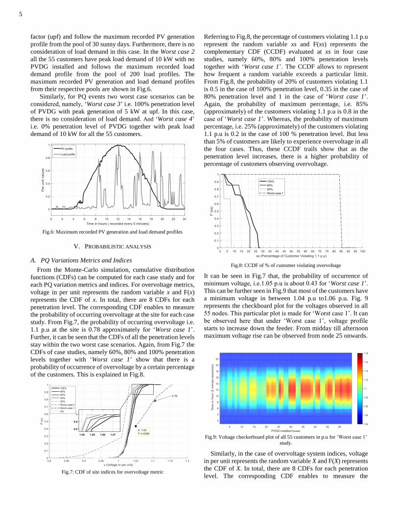
factor (upf) and follow the maximum recorded PV generation

profile from the pool of 30 sunny days. Furthermore, there is no

consideration of load demand in this case. In the Worst case 2

all the 55 customers have peak load demand of 10 kW with no

PVDG installed and follows the maximum recorded load

demand profile from the pool of 200 load profiles. The

maximum recorded PV generation and load demand profiles

from their respective pools are shown in Fig.6.

Similarly, for PQ events two worst case scenarios can be

considered, namely, ‘Worst case 3’ i.e. 100% penetration level

of PVDG with peak generation of 5 kW at upf. In this case,

there is no consideration of load demand. And ‘Worst case 4’

i.e. 0% penetration level of PVDG together with peak load

demand of 10 kW for all the 55 customers.

Fig.6: Maximum recorded PV generation and load demand profiles

V. PROBABILISTIC ANALYSIS

A. PQ Variations Metrics and Indices

From the Monte-Carlo simulation, cumulative distribution

functions (CDFs) can be computed for each case study and for

each PQ variation metrics and indices. For overvoltage metrics,

voltage in per unit represents the random variable x and F(x)

represents the CDF of x. In total, there are 8 CDFs for each

penetration level. The corresponding CDF enables to measure

the probability of occurring overvoltage at the site for each case

study. From Fig.7, the probability of occurring overvoltage i.e.

1.1 p.u at the site is 0.78 approximately for ‘Worst case 1’.

Further, it can be seen that the CDFs of all the penetration levels

stay within the two worst case scenarios. Again, from Fig.7 the

CDFs of case studies, namely 60%, 80% and 100% penetration

levels together with ‘Worst case 1’ show that there is a

probability of occurrence of overvoltage by a certain percentage

of the customers. This is explained in Fig.8.

Fig.7: CDF of site indices for overvoltage metric

Referring to Fig.8, the percentage of customers violating 1.1 p.u

represent the random variable xs and F(xs) represents the

complementary CDF (CCDF) evaluated at xs in four case

studies, namely 60%, 80% and 100% penetration levels

together with ‘Worst case 1’. The CCDF allows to represent

how frequent a random variable exceeds a particular limit.

From Fig.8, the probability of 20% of customers violating 1.1

is 0.5 in the case of 100% penetration level, 0.35 in the case of

80% penetration level and 1 in the case of ‘Worst case 1’.

Again, the probability of maximum percentage, i.e. 85%

(approximately) of the customers violating 1.1 p.u is 0.8 in the

case of ‘Worst case 1’. Whereas, the probability of maximum

percentage, i.e. 25% (approximately) of the customers violating

1.1 p.u is 0.2 in the case of 100 % penetration level. But less

than 5% of customers are likely to experience overvoltage in all

the four cases. Thus, these CCDF trails show that as the

penetration level increases, there is a higher probability of

percentage of customers observing overvoltage.

Fig.8: CCDF of % of customer violating overvoltage

It can be seen in Fig.7 that, the probability of occurrence of

minimum voltage, i.e.1.05 p.u is about 0.43 for ‘Worst case 1’.

This can be further seen in Fig.9 that most of the customers have

a minimum voltage in between 1.04 p.u to1.06 p.u. Fig. 9

represents the checkboard plot for the voltages observed in all

55 nodes. This particular plot is made for ‘Worst case 1’. It can

be observed here that under ‘Worst case 1’, voltage profile

starts to increase down the feeder. From midday till afternoon

maximum voltage rise can be observed from node 25 onwards.

Fig.9: Voltage checkerboard plot of all 55 customers in p.u for ‘Worst case 1’

study.

Similarly, in the case of overvoltage system indices, voltage

in per unit represents the random variable X and F(X) represents

the CDF of X. In total, there are 8 CDFs for each penetration

level. The corresponding CDF enables to measure the

6

probability of occurrence of overvoltage at the site for each case

study. From Fig.10, the probability of occurrence of

overvoltage (i.e. 1.1 p.u) at the system is 0 for all the 8 cases.

But the probability of occurrence of minimum voltage of 1.045

p.u is 0.4 in the case of ‘Worst case 1’. This can be further seen

in Fig.11 that the minimum voltage for all the three phase

voltages at substation transformer is about 1.04 p.u in the case

of ‘Worst case 1’.

Fig.10: CDF of system indices for overvoltage metric

Fig.11: Three phase voltages at substation transformer

For each index, the unbalance factor is computed and quantified

against the standard i.e. the voltage unbalance factor should be

less than 2% for 95% of a defined period. The unbalance site

indices are computed at the three-phase node where the

customers connect their single-phase service cable. Therefore,

there are 55 three phase nodes to consider for site voltage

unbalance. To quantify the percentage of occurrence of voltage

unbalance that exceeds a defined threshold limit, a cumulative

plot of voltage unbalance factor versus percentage of

occurrence (i.e. duration) are shown in Figures 12 and 13. These

graphs are essentially a CCDF. Fig. 12 shows the site voltage

unbalance factor for 8 different cases. It can be seen here that

the percentage of occurring the voltage unbalance factor of

almost 1.8 is 60% in the three cases, namely, 0% penetration

level, ‘Worst case 1’ and ‘Worst case 2’. This increase in

voltage unbalance at 0% penetration is a normal due to

unbalance loading in the LVDN. However, ‘Worst case 1’ and

‘Worst case 2’ are the extreme conditions and stays within the

limit. The percentage of occurring maximum voltage unbalance

factor of 1.907 is 54.3% in the case of ‘Worst case 1’. And, the

percentage of occurring maximum voltage unbalance factor of

1.821 is 41.29% in the case of ‘Worst case 2’. The unbalance

factor primarily depends on the loading in each phase. It can be

recalled that out of the 55 customers, phases A, B and C

accommodate 38.2%, 34.5% and 27.3% of the loads

respectively, showing a certain level of balance loading and is

shown in Fig.12 as 0% penetration.

A further observation from Fig.12 shows that the integration

of PVDG reduces the voltage unbalance factor. This is

primarily due to the phase cancellation between the phases. But

as the PVDG penetration increases from 20% to 100%, the

voltage unbalance factor starts to increase by a small factor. The

percentage of occurring maximum voltage unbalance factor of

about 1 to 1.2 is 100% of all the 8 cases. This means that most

of the time the voltage unbalance factor at each three phase

nodes will be within 1-1.2 meaning it will stay within the limit.

Overall, it can be concluded here that, PVDG integration

alleviates voltage unbalance in the LVDN.

Fig.12: Percentage of site voltage unbalance factor

The system index voltage unbalance factor is shown in Fig.

13. The unbalance factor is within the limit for all the 8 cases.

Similarly, here, as the penetration of PVDG increases from 0%

to 100%, the voltage unbalance increases by a small factor. The

percentage of occurring minimum voltage unbalance factor of

0.74 is 44.44% in the case of ‘Worst case 1’. And, the

percentage of occurring minimum voltage unbalance factor of

0.72 is 18.75% in the case of ‘Worst case 2’. Further, the

percentage of occurring maximum voltage unbalance factor of

about 0.7 to 0.75 is 100% of all the 8 cases. This means that

most of the time the voltage unbalance factor at the transformer

will be within 0.7 to 0.75. Overall, the voltage unbalance at the

transformer will be within the limit in all the 8 cases.

Fig.13: Percentage of site voltage unbalance factor

7

B. PQ Events Metrics and Indices

From the Monte-Carlo simulation, cumulative distribution

functions (CDFs) can be computed for each case study and for

each PQ event metrics and indices. As discussed earlier, the

observed voltage sags will be represented as a percentage of the

remaining voltage due to Monte-Carlo fault study. For voltage

sags site index, the remaining voltage represents the random

variable y and F (y) represents the CDF of y. The corresponding

CDF enables to measure the probability of observing certain

percentage of the remaining voltage for a particular case study.

Higher percentage of remaining voltage means it is a shallow

sag i.e. the low fault current. Whereas, lower percentage of

remaining voltage means it is a deep sag i.e. high fault current.

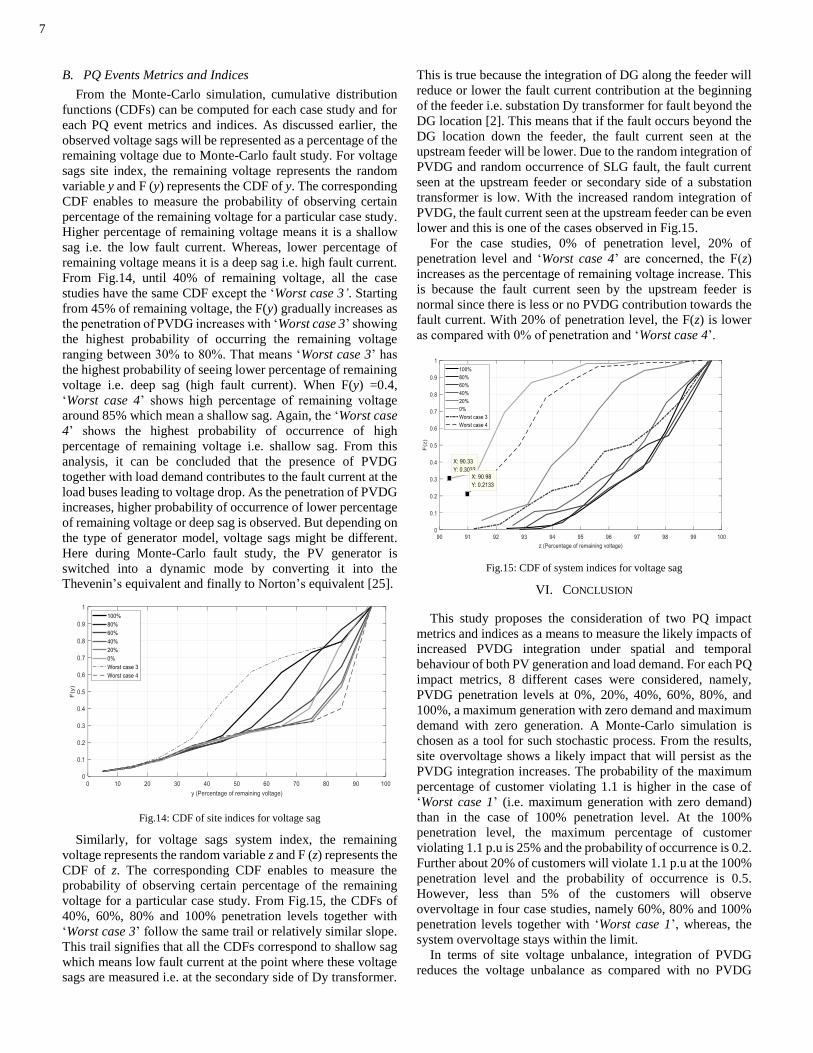
From Fig.14, until 40% of remaining voltage, all the case

studies have the same CDF except the ‘Worst case 3’. Starting

from 45% of remaining voltage, the F(y) gradually increases as

the penetration of PVDG increases with ‘Worst case 3’ showing

the highest probability of occurring the remaining voltage

ranging between 30% to 80%. That means ‘Worst case 3’ has

the highest probability of seeing lower percentage of remaining

voltage i.e. deep sag (high fault current). When F(y) =0.4,

‘Worst case 4’ shows high percentage of remaining voltage

around 85% which mean a shallow sag. Again, the ‘Worst case

4’ shows the highest probability of occurrence of high

percentage of remaining voltage i.e. shallow sag. From this

analysis, it can be concluded that the presence of PVDG

together with load demand contributes to the fault current at the

load buses leading to voltage drop. As the penetration of PVDG

increases, higher probability of occurrence of lower percentage

of remaining voltage or deep sag is observed. But depending on

the type of generator model, voltage sags might be different.

Here during Monte-Carlo fault study, the PV generator is

switched into a dynamic mode by converting it into the

Thevenin’s equivalent and finally to Norton’s equivalent [25].

Fig.14: CDF of site indices for voltage sag

Similarly, for voltage sags system index, the remaining

voltage represents the random variable z and F (z) represents the

CDF of z. The corresponding CDF enables to measure the

probability of observing certain percentage of the remaining

voltage for a particular case study. From Fig.15, the CDFs of

40%, 60%, 80% and 100% penetration levels together with

‘Worst case 3’ follow the same trail or relatively similar slope.

This trail signifies that all the CDFs correspond to shallow sag

which means low fault current at the point where these voltage

sags are measured i.e. at the secondary side of Dy transformer.

This is true because the integration of DG along the feeder will

reduce or lower the fault current contribution at the beginning

of the feeder i.e. substation Dy transformer for fault beyond the

DG location [2]. This means that if the fault occurs beyond the

DG location down the feeder, the fault current seen at the

upstream feeder will be lower. Due to the random integration of

PVDG and random occurrence of SLG fault, the fault current

seen at the upstream feeder or secondary side of a substation

transformer is low. With the increased random integration of

PVDG, the fault current seen at the upstream feeder can be even

lower and this is one of the cases observed in Fig.15.

For the case studies, 0% of penetration level, 20% of

penetration level and ‘Worst case 4’ are concerned, the F(z)

increases as the percentage of remaining voltage increase. This

is because the fault current seen by the upstream feeder is

normal since there is less or no PVDG contribution towards the

fault current. With 20% of penetration level, the F(z) is lower

as compared with 0% of penetration and ‘Worst case 4’.

Fig.15: CDF of system indices for voltage sag

VI. CONCLUSION

This study proposes the consideration of two PQ impact

metrics and indices as a means to measure the likely impacts of

increased PVDG integration under spatial and temporal

behaviour of both PV generation and load demand. For each PQ

impact metrics, 8 different cases were considered, namely,

PVDG penetration levels at 0%, 20%, 40%, 60%, 80%, and

100%, a maximum generation with zero demand and maximum

demand with zero generation. A Monte-Carlo simulation is

chosen as a tool for such stochastic process. From the results,

site overvoltage shows a likely impact that will persist as the

PVDG integration increases. The probability of the maximum

percentage of customer violating 1.1 is higher in the case of

‘Worst case 1’ (i.e. maximum generation with zero demand)

than in the case of 100% penetration level. At the 100%

penetration level, the maximum percentage of customer

violating 1.1 p.u is 25% and the probability of occurrence is 0.2.

Further about 20% of customers will violate 1.1 p.u at the 100%

penetration level and the probability of occurrence is 0.5.

However, less than 5% of the customers will observe

overvoltage in four case studies, namely 60%, 80% and 100%

penetration levels together with ‘Worst case 1’, whereas, the

system overvoltage stays within the limit.

In terms of site voltage unbalance, integration of PVDG

reduces the voltage unbalance as compared with no PVDG

8

integration or low penetration level. This is mainly due to the

phase cancellation. This increase in voltage unbalance at 0%

penetration is a normal due to unbalance loading in the LVDN.

Overall, the site and system voltage unbalance stay within the

limit for all the 8 different cases. In the case of site voltage sag,

as the penetration of PVDG increases, higher probability of

occurrence of lower percentage of remaining voltage or deep

sag is observed. However, the system voltage sags are quite

different from that of the site. The probability of occurrence of

lower remaining voltage or deep sag reduces as the penetration

of PVDG increases. This is because PVDG integration reduces

the fault current seen at the upstream feeder.

In conclusion, the increased integration of PVDG poses some

threat to the performance of the power system. From the

probabilistic study, overvoltage poses the highest threat,

whereas voltage unbalance stays within the limit. Further,

increased integration of PVDG will contribute towards fault

current leading to deep sag at the site. This probabilistic

approach can be used as a tool to identify the likely impacts due

to PVDG integration at the existing load buses. This will enable

in quantifying the likely impacts against the worst-case

scenarios.

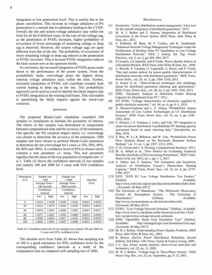
APPENDIX

The proposed Monte-Carlo simulation considerd 100

samples or simulations to estimate the parameter of interest.

The choice of this samples was determined to compromise

between computational time and the accuracy of the estimation.

One specific site PQ variation impact metric i.e. overvoltage

was chosen to determine the accuracy of the estimation. 1000

samples size have chosen to perform Monte-Carlo simulation

to determine the site overvoltage for 5 cases i.e. 0%, 20%, 40%,

60, 80% and 100%. A confidence level of 95% is chosen which

contains a true parameter i.e. mean. This true parameter

signifies that the mean of the true population of samples size ‘n’

is 1. Table A1 shows the confidence intervals of two samples

size namely 100 and 1000 for 5 cases with 95% confidence

level.

Penetration

in %

Sample size

=100

Sample size

=1000

Absolute Error Average Time =

180 seconds

Average Time =

1800 seconds

Confidence

interval

Confidence

interval

low high low high low high

0 1.0316 1.0358 1.0329 1.0343 0.0013 0.0016

20 1.0332 1.0373 1.0345 1.0359 0.0014 0.0014

40 1.0353 1.0397 1.0366 1.0381 0.0013 0.0017

60 1.0377 1.0427 1.0392 1.0409 0.0015 0.0019

80 1.0396 1.0453 1.0417 1.0435 0.0021 0.0018

100 1.0426 1.0491 1.0447 1.0468 0.0021 0.0024

Table A1: Confidence intervals of two samples size namely 100 and 1000 for

5 cases with 95% confidence level

The absolute error from Table A1 shows that sampling size

of 100 is a good estimation for 95% confidence level for the

corresponding confidence intervals at a tenth of the

computation time as compared with sampling size of 1000.

REFERENCES

[1] Eurelectric, “Active distribution system management: A key tool

for the smooth integration of distributed generation,” 2013.

[2] M. H. J. Bollen and F. Hassan, Integration of Distributed

Generation in the Power System. IEEE Press, John Wiley &

Sons, Inc., 2011.

[3] S. Pukhrem, M. Basu, M. F. Conlon, and K. Sunderland,

“Enhanced Network Voltage Management Techniques Under the

Proliferation of Rooftop Solar PV Installation in Low-Voltage

Distribution Network,” IEEE J. Emerg. Sel. Top. Power

Electron., vol. 5, no. 2, pp. 681–694, 2017.

[4] P.Caramia, G.Carpinelli, and P.Verde, Power Quality Indices in

Liberalized Markets. IEEE Press, John Wiley & Sons, Inc., 2009.

[5] A. Bracale, P. Caramia, G. Carpinelli, A. Russo, and P. Verde,

“Site and system indices for power-quality characterization of

distribution networks with distributed generation,” IEEE Trans.

Power Deliv., vol. 26, no. 3, pp. 1304–1316, 2011.

[6] A. Keane et al., “State-of-the-art techniques and challenges

ahead for distributed generation planning and optimization,”

IEEE Trans. Power Syst., vol. 28, no. 2, pp. 1493–1502, 2013.

[7] EPRI, “Stochastic Analysis to Determine Feeder Hosting

Capacity for Distributed Solar PV,” 2011.

[8] EN 50160, “Voltage characteristics of electricity supplied by

public electricity networks,” vol. 44, no. 0, pp. 0–1, 2013.

[9] A. Navarro-Espinosa and L. F. Ochoa, “Probabilistic Impact

Assessment of Low Carbon Technologies in LV Distribution

Systems,” IEEE Trans. Power Syst., vol. 31, no. 3, pp. 2192–

2203, 2016.

[10] V. Klonari, J.-F. Toubeau, J. Lobry, and Vall, “PV integration in

smart city power distribution A probabilistic PV hosting capacity

assessment based on smart metering data,” Smartgreens, no.

May, 2016.

[11] Z. Ren, W. Li, R. Billinton, and W. Yan, “Probabilistic Power

Flow Analysis Based on the Stochastic Response Surface

Method,” vol. 31, no. 3, pp. 2307–2315, 2016.

[12] G. H. Givens and J. A. Hoeting, Computational Statistics. 2013.

[13] M. A. Akbari et al., “New Metrics for Evaluating Technical

Benefits and Risks of DGs Increasing Penetration,” IEEE Trans.

Smart Grid, vol. 3053, no. c, pp. 1–1, 2017.

[14] A. Dubey and S. Santoso, “On Estimation and Sensitivity

Analysis of Distribution Circuit’s Photovoltaic Hosting

Capacity,” IEEE Trans. Power Syst., vol. 32, no. 4, pp. 2779–

2789, 2017.

[15] IEEE, “IEEE EU Low Voltage Distribution Test Feeders.”

[Online]. Available:

http://www.ewh.ieee.org/soc/pes/dsacom/testfeeders/index.html

. [Accessed: 28-May-2017].

[16] The University of Manchester, “The Whitworth Observatory

(Centre for Atmospheric Science - The University of

Manchester).” [Online]. Available:

http://www.cas.manchester.ac.uk/restools/whitworth/.

[Accessed: 28-May-2017].

[17] ENWL, “Low Voltage Network Solutions.” [Online]. Available:

http://www.enwl.co.uk/about-us/the-future/nia-lcnf-tier-1/lcnf-

tier-1-projects/low-voltage-network-solutions.

[18] EPRI, “OpenDSS: Smart Grid Simulation Tool.” [Online].

Available: http://smartgrid.epri.com/SimulationTool.aspx.

[Accessed: 28-May-2017].

[19] M. H. J. Bollen, Understanding Power Quality Problems. IEEE

Press, John Wiley & Sons, Inc., 2001.

[20] R. Brown, Electric Power Distribution Reliability, Second

Edition, 2nd Editio. CRC Press, Taylor & Francis Group, 2009.

[21] J. C. Das, Power system analysis: short-circuit load flow and

harmonics, vol. 22, no. 12. 2002.

[22] M. H. J. Bollen, “Voltage Sags in Three-Phase System,” IEEE

Power Eng. Rev., vol. 21, no. September, pp. 8–15, 2001.

9

[23] W. L. Martinez and A. R. Martinez, Computational Statistics

handbook with MATLAB, Second Edition. Taylor & Francis

Group, 2007.

[24] R. C. Dugan, “OpenDSS Fault Study Mode.” 2003.

[25] EPRI, “OpenDSS Manual,” 2016.

Shivananda Pukhrem (S’18) received

B.E (Hons) degree in Electrical and

Electronics Engineering from

Visvesvaraya Technological University,

Belgaum, India in 2011 and M.Sc. Degree

in Renewable Energy System from

Wroclaw University of Technology,

Poland in 2013. He is currently pursuing

the Ph.D. degree in electrical engineering

at the School of Electrical and Electronic Engineering at Dublin

Institute of Technology (DIT), Dublin, Ireland.

From 2014 to 2016 he was involved in EU FP7 project

entitled “PV CROPS”. His PhD research endeavour includes an

active planning and operation for improving the high share of

non-firm DG integration in public distribution network. Mr.

Pukhrem is a student member of CIGRE.

Malabika Basu (S’99–M’03) received the

B.E. and M.E. degrees in electrical

engineering from Bengal Engineering

College, Shibpur, Kolkata, India, in 1995

and 1997, respectively, and the Ph.D.

degree in electrical engineering from

Indian Institute of Technology, Kanpur,

Uttar Pradesh, India, in 2003.

From 2001 to 2003, she was a Lecturer in Jadavpur

University, Kolkata, West Bengal, India. From 2003 to 2006,

she was Arnold F. Graves Postdoctoral Fellow at Dublin

Institute of Technology, Dublin, Ireland, where she has been a

Lecturer, since 2006. She has authored or co-authored more

than 80 technical publications in various international journals

and conference proceedings. Her current research interests

include grid integration of renewable energy sources, power

quality conditioners and power quality control and analysis,

photovoltaics and wind energy conversion, and smart grid and

microgrids.

Michael F. Conlon (M’88) received the

Dip.E.E., B.Sc. from Dublin Institute of

Technology, Dublin, Ireland, in 1982, the

M.Eng.Sc. degree by research and the

Ph.D. degree from the University College,

Galway, Ireland, in 1984 and 1987,

respectively, all in electrical engineering.

Prof. Michael Conlon is the Head of the

School of Electrical and Electronic Engineering at the Dublin

Institute of Technology, Kevin St, Dublin. He is Director of the

Electrical Power Research Centre (EPRC) in DIT. He was

previously with Monash University and VENCorp in

Melbourne, Australia. His research interests include power

systems analysis and control applications; power systems

economics; integration of wind energy in power networks;

analysis of distribution networks; quality of supply and

reliability assessment.