ww.sciencedirect.com

wat e r r e s e a r c h 5 0 ( 2 0 1 4 ) 2 5 4e2 6 6

Available online at w

ScienceDirect

journal homepage: www.elsevier .com/locate /watres

Probabilistic parameter estimation of activatedsludge processes using Markov Chain Monte Carlo

Soroosh Sharifi a,1, Sudhir Murthy b, Imre Takacs c, Arash Massoudieh a,*aCivil Engineering, The Catholic University of America, 630 Michigan Ave NE, Washington, DC 20064, USAbDC Water and Sewer Authority, 5000 Overlook Avenue, SW, Washington, DC 20032, USAcDynamita, 7 lieu-dit Eoupe, 26110 Nyons, France

a r t i c l e i n f o

Article history:

Received 15 August 2013

Received in revised form

23 November 2013

Accepted 5 December 2013

Available online 15 December 2013

Keywords:

ASM

Biological treatment

Bayesian

Markov Chain Monte Carlo

Uncertainty assessment

* Corresponding author.E-mail addresses: S.Sharifi@bham.ac.uk (

1 Current address: School of Civil Engineer0043-1354/$ e see front matter ª 2013 Elsevhttp://dx.doi.org/10.1016/j.watres.2013.12.010

a b s t r a c t

One of the most important challenges in making activated sludge models (ASMs) applicable

to design problems is identifying the values of its many stoichiometric and kinetic pa-

rameters. When wastewater characteristics data from full-scale biological treatment sys-

tems are used for parameter estimation, several sources of uncertainty, including

uncertainty in measured data, external forcing (e.g. influent characteristics), and model

structural errors influence the value of the estimated parameters. This paper presents a

Bayesian hierarchical modeling framework for the probabilistic estimation of activated

sludge process parameters. The method provides the joint probability density functions

(JPDFs) of stoichiometric and kinetic parameters by updating prior information regarding

the parameters obtained from expert knowledge and literature. The method also provides

the posterior correlations between the parameters, as well as a measure of sensitivity of

the different constituents with respect to the parameters. This information can be used to

design experiments to provide higher information content regarding certain parameters.

The method is illustrated using the ASM1 model to describe synthetically generated data

from a hypothetical biological treatment system. The results indicate that data from full-

scale systems can narrow down the ranges of some parameters substantially whereas

the amount of information they provide regarding other parameters is small, due to either

large correlations between some of the parameters or a lack of sensitivity with respect to

the parameters.

ª 2013 Elsevier Ltd. All rights reserved.

1. Introduction

Since its introduction in 1987, IWA’s Activated Sludge Model 1

(ASM1) (Henze et al., 1987) and its successors have become

extensively popular for the design and optimization of bio-

logical treatment systems (Gernaey et al., 2004; Sin et al.,

S. Sharifi), arashmassoud

ing, University of Birminier Ltd. All rights reserve

2005). As mechanistic models, the main goal of ASMs is to

predict the performance of biological treatment processes in

removing organic matter and nutrients under different con-

ditions. When applying ASMs to design or optimize biological

treatment processes, it is important to recognize and quantify

the uncertainties associated with the model outputs (Belia

et al., 2009). The main sources of uncertainty in ASM

ieh@gmail.com, massoudieh@cua.edu (A. Massoudieh).

gham, Edgbaston, Birmingham B15 2TT, UK.d.

wat e r r e s e a r c h 5 0 ( 2 0 1 4 ) 2 5 4e2 6 6 255

modeling can be categorized into four main groups (Cierkens

et al., 2012):

1) Model input data uncertainty, i.e., uncertainties associated

with influent characterization or environmental factors

such as temperature.

2) Uncertainty in model parameters.

3) Model structural error, due to the fact that the model is, at

best, an idealization of the real process.

4) Uncertainty associated with the numerical methods used

within the model (truncation errors).

Arguably, the most important challenge in making ASM

models usable in practice is attributing the values of its many

stoichiometric and kinetic parameters (Gernaey et al., 2004)d

hereafter, for the sake of simplicity, referred to as “parame-

ters”dwhich sometimes cannot be measured directly

(Weijers and Vanrolleghem, 1997). Usually, when ASMs are

used for practical purposes, the values of kinetic and stoi-

chiometric parameters, such as biomass growth rates, yield

coefficients, and half-saturation constants, are determined

based on the values provided in the literature. The literature

values are obtained through independent batch or other types

of experiments under controlled conditions or by using pre-

vious model calibrations based on data from full-scale sys-

tems. Because different parameter values are suggested by

different studies, a range of values for each parameter is often

reported (Jeppsson, 1996). These ranges are sometime so wide

that choosing different parameterswithin the range can result

in drastically different predictions. Lab experiments under

controlled conditions often require several series of mea-

surements of constituents of interest under a range of other

influencing factors, while keeping other factors constant

(Amano et al, 2002). The values obtained under these condi-

tions are not always applicable to full-scale bioreactors, due to

broader heterogeneities and the interactions of larger

numbers of components, including a more diverse set of

chemical and bacterial species. On the other hand, when

manual calibration is used to estimate ASMmodel parameters

using data collected from full-scale systems, it is not guar-

anteed that the obtained set of parameters is the only

parameter-set, resulting in reproduction of the observed data.

This problem has been referred to as non-uniqueness, lack of

identifiability, or equifinality (Beven and Freer, 2001). This is

due to the fact that ASMs are generally over-parameterized

with respect to the amount of data available for calibration,

and because, under certain operational bioreactor conditions,

the effluent characteristics can be insensitive to the values of

some of the parameters (Cierkens et al., 2012).

Automatic and semi-automatic deterministic methods

based on least-squares and maximum likelihood criteria (e.g.,

linearized maximum likelihood (Kabouris and Georgakakos,

1996a, b)) have been used to estimate the optimal values of

ASM parameters using observed data. Gradient-based (e.g.,

generalized reduced gradient method (Afonso and da

Conceicao Cunha, 2002)) and heuristic search methods (e.g.,

Simplex techniques (Cierkens et al., 2012)) have been used

extensively in the past to determine ASM parameters. Ayesa

et al. (1991) used the extended Kalman filter to estimate ASM

parameters as time-dependent parameters. Vanrolleghem

and Keesman (1996) compared a number of nonlinear

parameter estimation methods for identifying ASM parame-

ters and suggested the use of Monte Carlo simulations. Sin

et al. (2008) used a Monte Carlo-based search algorithm to

estimate the ASM parameters. Cox (2004) compiled a few da-

tabases containing the values of the parameters of ASM and

used a Bayesian approach to develop statistical distributions

for them. Gradient-based methods are prone to getting trap-

ped in a local optima (Abusam et al., 2001), and sometimes,

parameter values thatmay not be physically interpretable end

up being found (Weijers and Vanrolleghem, 1997). In addition,

while deterministic methods might provide a parameter set

that maximizes the chance of reproducing the observed data,

they are incapable of providing any reliability measure for the

estimated parameter values.

The complexity involved in the calibration of ASMs has led

to a number of protocols and guidelines for manual system-

atic calibration of full-scale ASM systems. BIOMATH (Petersen

et al., 2002; 2003; Vanrolleghem et al., 2003), STOWA (Hulsbeek

et al., 2002), HSG (Langergraber et al., 2004), WERF (Melcer

et al., 2003), and IWA’s STR (Rieger et al., 2012) are among

themost well-known protocols. These all consist of four main

steps: 1) characterizing influent wastewater; 2) constructing

dynamic influent loading data; 3) manual parameter estima-

tion; and 4) model validation. A critical comparison of these

methods can be found in (Sin et al., 2005).

Almost all of the approaches used for the automatic cali-

bration of ASMs have been deterministic so far with the

exception of the work of Juznic et al. (2001), who applied

Bayesian inference to estimate parameter uncertainty asso-

ciated with a revised version of ASM3 and showed its advan-

tage over some deterministic linear theory methods. In

deterministic parameter estimation approaches one set of

parameter values often as a results minimization between

some measures of misfit between the modeled and measured

results is obtained using a manual or automated optimization

technique. However, many sources of uncertainty and error,

including observation error, model structural error, errors

associated with input variables and external forcing, and

possible non-uniqueness of optimum parameters or lack of

sensitivity of the predicted effluent concentrations to certain

parameters under some conditions, are inevitably propagated

into the estimated parameters and need to be quantified.

Deterministic parameter estimation approaches provide a

single set of parameters, and it is not clear how much devia-

tion from those estimated values is still acceptable and what

the shape of the region of plausibility in the parameter space

looks like. Regardless of what calibration method is used,

parameter uncertainty is always present and eventually

transmits into model output uncertainty (Morgan and

Henrion, 1992). Using a single set of parameters to obtain

some model outputs could result in the sub-optimal design of

biological treatment systems, incorrect planning decisions,

and poor effluent water quality. Therefore, to use the ASMs

effectively for optimization of the operation and design of

biological treatment systems, it is necessary that the effects of

these uncertainties on the uncertainties of parameter esti-

mation to be quantified.

Various uncertainty quantification approaches have been

used in various scientific fields. These include local sensitivity

wat e r r e s e a r c h 5 0 ( 2 0 1 4 ) 2 5 4e2 6 6256

approaches based on multiple linear regression that are

established on the assumption of a linear dependence of the

model outputs and parameters (e.g. Hill and Tiedeman, 2007;

Foglia et al., 2009), global methods such as Generalized Like-

lihood Uncertainty Estimator, GLUE, (Beven and Freer, 2001)

and Bayesian inference. Local sensitivity analysis is not able to

capture the effects of non-linear dependence of outputs to the

parameters, but on the other hand, requires a much smaller

number of model runs to perform the uncertainty quantifi-

cation. The GLUE methodology uses a subjective measure of

likelihood based on a metric of goodness of fit to assign

different levels of confidence to different parameter sets. It

requires a large number of model evaluations to generate re-

alizations of model outputs using parameters sampled from

(often) uniform distributions over the plausible range of each

parameter. In the Bayesian approach the joint probability

distribution of parameters after conditioning them to the data

and prior knowledge about the parameters (referred to as

posterior distribution) is obtained based on the formal Bayes

theorem. Markov Chain Monte Carlo (MCMC) methods can

then be used to draw large number of samples from this

posterior distribution. The robustness of the Bayesian

approach compared to other methods has been demonstrated

in several studies (e.g Makowski et al., 2002; Gallagher and

Doherty, 2007). Both GLUE and MCMC approaches require a

much larger of model runs compared to the local sensitivity

methods.

Bayesian modeling allows incorporation of prior knowl-

edge regarding the parameters; for example, from past lab

experiments or ranges of parameters provided in the litera-

ture. The resulting joint PDFs of the parameters can be used in

conjunction with Monte Carlo simulation techniques to

perform probabilistic designs and controls of biological

treatment systems, while taking into consideration the

parameter uncertainty. Another advantage of Bayesian

parameter estimation is that, as further data is obtained, it can

be used to update the posterior parameter probability

distributions.

In this study, the development of a Markov Chain Monte

Carlo (MCMC) method based on Bayesian hierarchical

modeling for the probabilistic parameter estimation of acti-

vated sludge systems is described. To demonstrate the

application of the method, this is used for calibrating the

ASM1 using synthetic data obtained from a test case adopted

from the literature.

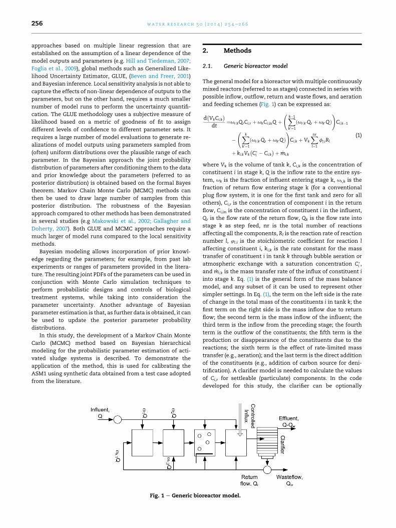
Fig. 1 e Generic bio

2. Methods

2.1. Generic bioreactor model

The generalmodel for a bioreactor withmultiple continuously

mixed reactors (referred to as stages) connected in series with

possible inflow, outflow, return and waste flows, and aeration

and feeding schemes (Fig. 1) can be expressed as:

d�VkCi;k

�dt

¼ur;kQrCi;r þ ukCi;inQ þ Xk�1

k0¼1

ður;k0Qr þ uk0QÞ!Ci;k�1

� Xk

k0¼1

ður;k0Qr þ uk0QÞ!Ci;k þ Vk

Xnrl¼1

fl:iRl

þ ki;kVk

�C�i � Ci;k

�þ _mi;k

(1)

where Vk is the volume of tank k, Ci,k is the concentration of

constituent i in stage k, Q is the inflow rate to the entire sys-

tem, uk is the fraction of influent entering stage k, ur,k is the

fraction of return flow entering stage k (for a conventional

plug flow system, it is one for the first tank and zero for all

others), Ci,r is the concentration of component i in the return

flow, Ci,in is the concentration of constituent i in the influent,

Qr is the flow rate of the return flow, Qk is the flow rate into

stage k as step feed, nr is the total number of reactions

affecting all the components, Rl is the reaction rate of reaction

number l, 4l.i is the stoichiometric coefficient for reaction l

affecting constituent i, ki,k is the rate constant for the mass

transfer of constituent i in tank k through bubble aeration or

atmospheric exchange with a saturation concentration C�i ,

and _mi;k is the mass transfer rate of the influx of constituent i

into stage k. Eq. (1) is the general form of the mass balance

model, and any subset of it can be used to represent other

simpler settings. In Eq. (1), the term on the left side is the rate

of change in the total mass of the constituents i in tank k; the

first term on the right side is the mass inflow due to return

flow; the second term is the mass inflow of the influent; the

third term is the inflow from the preceding stage; the fourth

term is the outflow of the constituents; the fifth term is the

production or disappearance of the constituents due to the

reactions; the sixth term is the effect of rate-limited mass

transfer (e.g., aeration); and the last term is the direct addition

of the constituents (e.g., addition of carbon source for deni-

trification). A clarifier model is needed to calculate the values

of Ci,r for settleable (particulate) components. In the code

developed for this study, the clarifier can be optionally

reactor model.

wat e r r e s e a r c h 5 0 ( 2 0 1 4 ) 2 5 4e2 6 6 257

represented by assuming zero solid concentration in the

effluent and quasi steady-state approximation (i.e. perform-

ing mass balance while ignoring the solid storage changes in

the clarifier), or by the dynamic clarifier model proposed by

Takacs et al. (1991). In addition, in the biological reaction

network used for modeling the reactors, the code allows any

reaction rate expression Rl and stoichiometric constant 4l.i to

be specified by the user as a function of concentrations of

components and model parameters.

2.2. Bayesian parameter estimation

Equation (1) can be expressed in a more general form as:

dCdt

¼ fðCðtÞ;UðtÞ;QÞ (2)

eCðtÞ ¼ gðCðtÞ; εÞ (3)

where C(t) is the state variable vector representing the con-

centrations of various components in the reactor (here also

referred to as the true concentration), U(t) is the input (or

external forcing vector), Q is the parameter vector, eCðtÞ is the

observed data vector, and ε contains some measures repre-

senting the random observation error. In Eqs. (2) and (3),

function f represents the bioreactor model structure, and g

represents the output error structure. When observations at

certain time intervals are available, eCðtÞ and C(t) can be rep-

resented as matrices, with eC ¼ ½~cij� containing the values of

observed constituents i at data point j, and C ¼ [cij] containing

modeled constituent concentrations at the same times.

The goal of stochastic parameter estimation is to find the

joint distribution of the parameters, Q, given observed

external forcing U(t) and observed values eC. In a Bayesian

framework, the joint probability distribution of the parame-

ters after incorporating the observations (posterior distribu-

tion) can be expressed through Bayes’ theorem (Kaipio and

Somersale, 2004):

P�Q;G

��eC� ¼ P�eC��Q;G

�$PðQ;GÞ

P�eC� (4)

where G ¼ [sik] is the variance-covariance matrix of the

observation error between the concentrations of different

constituents and its elements, with each element, sik, being

the covariance between the concentrations of constituents i

and k. In Eq. (4), the first term in the numerator on the right

side is the likelihood function that represents the probability

of seeing the observed concentrations, given the true values of

the parameters; the second term in the numerator is the prior

density, which contains the prior knowledge about the values

of the parameters; and finally, the denominator is a normal-

izing factor referred to as evidence. If we make an assumption

about the observed error structure, g, given the ASM, the

likelihood function can be expressed as:

P�eC��Q;G

�¼ P

heC��CðQ;UðtÞÞ;Gi

(5)

For example, if it is assumed that the observed error fol-

lows a Gaussian distribution, then the likelihood function can

be written as:

�e�� � 1

0B Xn �~Cj � Cj

�G�1

�~Cj � Cj

�T1C

P C C;G ¼ð2pjGjÞn=2

exp@�j¼1

2A (6)

or if the error structure is assumed to be log-normal and

multiplicative, the likelihood function becomes:

P�eC��C;Gln

�¼ 1 Ym

i¼1

Ynj¼1

cij

1Að2pjGlnjÞn=2exp

�0@�

Xnj¼1

hln�~Cj

�� ln

�Cj

�iG�1

ln

hln�~Cj

�� ln

�Cj

�iT2

1A(7)

In Eq. (7), Gln is the variance-covariance matrix of the log-

transformed concentrations of constituent concentrations.

In practice, all of the elements of the variance-covariance

matrix need to be estimated using the MCMC approach.

Since this makes the total number of parameters to be esti-

mated very large and imposes a very large computational

burden, the observation errors are typically assumed to be

independent, and the correlation between the observed con-

centration errors are ignored (Walsh and Whitney, 2012). By

making this assumption, the variance-covariance matrix be-

comes a diagonal matrix:

G ¼

2664s21

s22

:s2m

3775 (8)

where si is the error standard deviation for constituent i. In a

log-normal multiplicative error structure for observed

concentrations:

Gln ¼

2664s2ln;1

s2ln;2

:s2ln;m

3775 (9)

where sln,i is the standard deviation of log-transformed con-

centrations of constituents i. Incorporating Eqs. (8) and (9) into

Eqs. (6) and (7), respectively, results in:

P�eC��C;G� ¼ 1

ð2pÞn=2�Ym

i¼1

si

!n exp

0@�Xnj¼1

Xmi¼1

�~cij � cij

�22s2

i

1A (10)

and

P�eC��C;Gln

�¼ 1 Ym

i¼1

Ynj¼1

cij

1Að2pÞn=2 Ym

i¼1

sln;i

!nexp

�0@�

Xnj¼1

Xmi¼1

�ln�~cij�� ln

�cij�2

2s2ln;i

1A (11)

Assuming that the prior distributions of the parameters are

also independent, the prior distribution can be written as:

PðQ;GÞ ¼Ymi¼1

PðqiÞ$Ymi¼1

P�sðlnÞi

�(12)

wat e r r e s e a r c h 5 0 ( 2 0 1 4 ) 2 5 4e2 6 6258

Furthermore, assuming that the prior distributions are

normal for some of the parameters and log-normal for others,

and considering the fact that no prior information about the

observation error standard deviations are available, Eq. (4) for

the two cases of normally and log-normally distributed

observation error becomes:

P�q1; q2;.; ql;G

��eC�f 1�Ymi¼1

si

!n exp

0@�Xnj¼1

Xmi¼1

�~cij � cij

�22s2

i

1A

�Yl1k¼1

e�ðqk�mkÞ2

2s2p;k

sp;k

Yl2k0¼1

e�ðln qk0 �mk0 Þ2

2s2p;k0

fk0sln;p;k0(13)

P�q1;q2;.;ql;GjeC�f 1�Ym

i¼1

sln;i

!nexp

0@�Xnj¼1

Xmi¼1

�ln�~cij��ln

�cij�2

2s2ln;i

1A

�Yl1k¼1

e�ðqk�mkÞ2

2s2p;k

sp;k

Yl2k0¼1

e�ðln qk0 �mk0 Þ2

2s2p;k0

fk0sln;p;k0(14)

where mk is the mean of the prior distribution of parameter qkand sp,k is its standard deviation.

In order to evaluate various moments or confidence in-

tervals of the posterior parameters, Eq. (4) needs to be inte-

grated over the domains of all parameters. Because it is not

feasible to do this practically, due to the large number of pa-

rameters, an MCMC method (Kaipio and Somersale, 2004;

Gamerman and Hedibert, 2006) is used to generate a large

number of samples from the posterior distribution. Having a

large number of samples according to the posterior distribu-

tion, we can effectively construct histograms representing

marginal distributions of the parameters. In this work, a

MetropoliseHastings algorithm (Metropolis et al., 1953) is used

to sample from Eqs. (13) or (14). The algorithm generates

Markov chains in which each new set of variables depends on

the previous set. The code developed in this study uses

normal or log-normal proposal densities Qðq0i; qkÞ according to

whether the prior densities of parameters are considered

normal or lognormal. The proposal densities are used to

generate proposal parameter sets Q0given the previous states

Qk. The proposal parameter set Q0is accepted as the next

value based on the following criteria:

Qkþ1 ¼

8><>:Q0 if Uð0;1Þ < min

PðQ0 ÞQðQ0 ;QkÞPðQkÞQðQk ;Q0Þ;1

�Qk otherwise

(15)

where U(0,1) is a uniformly distributed random number be-

tween 0 and 1 and P is the posterior probability density.

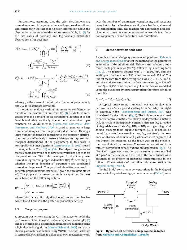
Fig. 2 e Hypothetical activated sludge system (adopted

from Kabouris and Georgakakos, 1996a,b).

2.3. Computer program

A program was written using the Cþþ language to model the

performanceof thebiological treatmentsystembysolvingEq. (1)

and to performboth adeterministic parameter estimationusing

a hybrid genetic algorithm (Massoudieh et al., 2008) and a sto-

chastic parameter estimation using MCMC. The code is flexible

in terms of allowing users to define their own reaction network,

with the number of parameters, constituents, and reactions

being limited by the hardware’s ability to solve the system and

the computation time. The reaction rate expressions and stoi-

chiometric constants can be expressed as user-defined func-

tions of parameters and constituent concentrations.

3. Demonstration test case

A simple activated sludge system was adopted from Kabouris

and Georgakakos (1996b) to test the method for the parameter

estimation of the ASM1 model. This system includes a fully

mixed biological reactor (CSTR), followed by a settling tank

(Fig. 2). The reactor’s volume was V ¼ 16,000 m3, and the

settling tank had an area of 790m2 and volumeof 1455m3. The

underflow rate from the settling tank was Q ¼ 18,350 m3/d,

and the sludge waste and return flow rates were Qw ¼ 600 m3/

d andQr¼ 17,750m3/d, respectively. The clarifierwasmodeled

using the quasi steady-state assumption; therefore, for all of

the solids:

Cr ¼ Cw ¼ CðQ þ QrÞ=ðQr þ QwÞ (16)

A typical time-varying municipal wastewater flow rate

pattern for a 4.5-day period starting from Saturday midnight

to Thursday noon (Tchobanoglous and Burton, 1991) was

considered for the influent (Fig. 3). The influent was assumed

to consist of five constituents: slowly biodegradable substrate

(XS), particulate biodegradable organic nitrogen (XND), readily

biodegradable substrate (SS), NH4 þ NH3 nitrogen (SNH), and

soluble biodegradable organic nitrogen (SND). It should be

noted that since the waste flow rate, Qw, was fixed, the pres-

ence or absence of soluble and particulate inert organics did

not impact the outcome, as the focus was on the stoichio-

metric and kinetic parameters. The assumed variations of the

influent component concentrations are depicted in Fig. 4. The

dissolved oxygen concentration was assumed to be controlled

at 6 g/m3 in the reactor, and the rest of the constituents were

assumed to be present in negligible concentrations in the

influent. Characteristics of the influent data are provided in

Supplementary Table 1.

To find initial constituent concentrations in the biological

tank, a set of reported average parameter values (Table 1) were

Fig. 3 e Influent wastewater flow.

wat e r r e s e a r c h 5 0 ( 2 0 1 4 ) 2 5 4e2 6 6 259

considered, and the ASM1was run to steady state using a fixed

flow rate and flow-weighted average inflow concentrations

until it reached steady-state conditions. Then, using the same

parameter set, the process was simulated using the varying

influent over a 4.5-day period, and a set of “perfect” mea-

surements for the effluent flow time series were obtained. To

generate a time series of realistic measured effluent concen-

trations, the measurements were “corrupted” by simulated

measurement noise. The noise was generated using a multi-

plicative and log-normally distributed first-order auto-

regressive (AR) process. The ARmodelwas used, as opposed to

white noise, in order to better resemble the model structural

error that is often auto-correlated (Yang et al., 2007). The noise

magnitude was selected to resemble the effects of the

different sources of uncertainties including the uncertainties

associated with observation error, model structural error and

input uncertainties in the model predictions. The developed

code can consider settling and aeration parameters as un-

known and estimate their distributions using observed data,

however, in the demonstration case here these parameters

were not included in the analysis.

4. Results

Tables 1 and 2 list the parameters and constituents, respec-

tively, of the ASM1. Eleven of the ASM1 parameters (values

specified as a range in Table 1) were considered parameters to

be estimated using the model, and the values of parameters

with single values (e.g., ka, kx) were considered fixed. It should

Fig. 4 e Concentration variation

be noted that other ranges for ASM1 parameters has been

proposed (e.g. Cox, 2004; Rieger et al., 2012; Benedetti et al.,

2012) in which the range of some of the parameters are

smaller and for some it is wider. Using alternative priors could

impact the estimated posterior parameter distributions. The

prior distributions of the parameters were considered log-

normally distributed with 95% confidence intervals given by

theminimum andmaximum ranges of the parameters shown

in Table 1. In this application, eight chains with a total length

of 5,000,000 samples were used, and the first 1,000,000 sam-

ples were disregarded as the “burn-in” period. The initial

conditions were established using the “true” parameter

values. The criteria suggested by Geweke and Tanizaki (2001)

were used to evaluate the convergence of the MCMC

algorithm.

Fig. 5 shows the obtained posterior distributions of the

ASM1 parameters. In this figure, the dashed line represents

the value of each parameter used to generate the synthetic

observation data, while the solid vertical line represents the

deterministic value of the parameter obtained using the ge-

netic algorithm through maximizing the likelihood function.

Due to a lack of sensitivity toward some of the parameters, a

possible correlation between the parameters, their non-

uniqueness, and the fact that genetic algorithms are not effi-

cient at finding the exact optima (Yuret, 1994), the determin-

istically estimated parameters do not match with the true

parameters. In addition, the noise added to the results of the

simulations used to generate the synthetic observation data

will result in parameter values different than the original

parameter values. However, as can be seen in Fig. 5, the his-

tograms representing the posterior distribution of the pa-

rameters are generally in good agreement with the true values

of the parameters. The level of confidence obtained for each

parameter depends on the confidence in the prior knowledge,

how much the value of that parameter can affect the effluent

concentration of water quality constituents and how close the

data on the effluent concentrations matches the expected

value of the predicted effluent concentrations. Table 3 con-

tains a measure of sensitivity of effluent constituent concen-

trations with respect to the parameters, as well as a measure

of the overall sensitivity of the model output with respect to

all the parameters, which is calculated as the sum of the

sensitivities of each constituent. The sensitivity of constituent

j with respect to parameter qi is calculated as:

s of influent components.

Table 1 e ASM1 model parameter ranges (Jeppsson, 1996).

Parameter Symbol Unit Literaturerange

Geometricaverage

Min Max

Stoichiometric parameters

Heterotrophic yield YH g cell COD formed (g COD oxidized)�1 0.380 e 0.750 0.534

Autotrophic yield YA g cell COD formed (g N oxidized)�1 0.070 e 0.280 0.140

Fraction of biomass yielding particulate products fP Dimensionless 0.080 0.080

Mass N/Mass COD in biomass ixB g N (g COD)�1 in biomass 0.086 0.086

Mass N/Mass COD in products from biomass ixP g N (g COD)�1 in endogenous mass 0.060 0.060

Kinetic parameters

Heterotrophic maximum specific growth rate mH 1/day 0.600 e 13.200 2.814

Heterotrophic decay rate bH 1/day 0.050 e 1.600 0.283

Half-saturation coefficient (hsc) for heterotrophs Ks g COD/m3 5 e 225 33.541

Oxygen hsc for heterotrophs KO,H g O2/m3 0.010 e 0.200 0.045

Nitrate hsc for denitrifying heterotrophs KNO g NO3eN/m3 0.100 e 0.500 0.224

Autotrophic maximum specific growth rate mA 1/day 0.200 e 1.000 0.447

Autotrophic decay rate bA 1/day 0.050 e 0.200 0.100

Oxygen hsc for autotrophs KO,A g O2/m3 0.400 e 2.000 0.894

Ammonia hsc for autotrophs KNH g NH3eN/m3 1.000 1.000

Correction factor for anoxic growth

of heterotrophs (mH)

sG Dimensionless 0.600 e 1.000 0.775

Ammonification rate ka m3/(g COD day) 0.080 0.080

Maximum specific hydrolysis rate kh g slowly biodeg. COD (g cell COD day)�1 3.000 3.000

Hsc for hydrolysis of slowly biodegradable substrate Kx g slowly biodeg. COD (g cell COD)�1 0.030 0.030

Correction factor for anoxic hydrolysis sh Dimensionless 0.400 0.400

wat e r r e s e a r c h 5 0 ( 2 0 1 4 ) 2 5 4e2 6 6260

I ¼Zts �

vln CjðtÞ�2

dt (17)

j;i

0vln qi

and the overall sensitivity of the model results with respect to

parameter i is:

Ii ¼Xj

Ij;i (18)

It should be noted that the sensitivitymeasures introduced

in Eqs. (17) and (18) are local sensitivities and are only appli-

cable to the close neighborhood of the maximum likelihood

solution and do not intend to represent the global sensitivity.

These measures are intended to be loosely considered as

surrogates for the sensitivity with respect to the parameters.

As can be seen, the greatest sensitivity is with respect to

yield coefficient for autotrophs (YA) followed by decay rate of

heterotrophs (bH) yield coefficient for heterotrophs (YH) and

growth rate of autotrophs (mA). The main reason for the large

Table 2 e ASM1 constituents.

Constituent Symbol Unit

Non-biodegradable soluble COD SI g COD/m3

Readily biodegradable substrate SS g COD/m3

Particulate non-biodegradable COD XI g COD/m3

Slowly biodegradable substrate XS g COD/m3

Heterotrophic biomass XB,H g COD/m3

Autotrophic biomass XB,A g COD/m3

Inert particulate product produced XP g COD/m3

Dissolved oxygen SO g O2/m3

Nitrate SNO g N/m3

Ammonia nitrogen SNH g N/m3

Soluble biodegradable organic nitrogen SND g N/m3

Particulate biodegradable organic nitrogen XND g N/m3

overall sensitivitywith respect to (YA) is its effect on ammonia.

This means that data on ammonia, particularly when a high

variation in ammonia is present, contains a great deal of in-

formation for the estimation of YA. bH has a large impact on

several constituents including Ss, Snd and Xnd. The effect of

and YH are spread among Ss and Snh while mA has the highest

effect on ammonia. It should be noted that sensitivity with

respect to a certain parameter does not translate directly into

high estimability for that parameter, as a large correlation

between the parameter and another parameter with a lower

sensitivity can result in a lower estimability. For example,

although the sensitivity with respect to YA is high, its estim-

ability is low, as shown in Fig. 5. In addition, a wide level of

confidence is obtained for the parameter through inverse

modeling, indicating low confidence. The reason for this is the

high correlation of YA with mA and bA. As shown in Fig. 5, the

marginal posterior distributions of some parameters,

including KOH, YH, and bH, are narrow, in spite of wide ranges

attributed to them in their prior distribution and the noise

added to the result of the synthetic simulation. This is because

of their high level of sensitivity and the lack of correlation

with other parameters (Fig. 6). It can also be seen that for these

three parameters, the deterministically estimated parameter

value is close to the true value. The lack of sensitivity toward

Kno is due to the fact that the oxygen level in this numerical

experiment was kept high to ensure that denitrificationwould

not occur.

Fig. 6 shows the pair-wise scatter plot samples of param-

eter values, and Table 4 shows the Pearson correlation matrix

for the parameters. For some parameters, strong correlations

can be observed. For example, there is a near one correlation

between the substrate half-saturation constant, Ks and the

maximum specific growth rate for mH. This high correlation is

due to the fact that in this study, the readily available

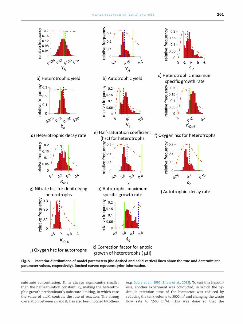
Fig. 5 e Posterior distributions of model parameters (the dashed and solid vertical lines show the true and deterministic

parameter values, respectively). Dashed curves represent prior information.

wat e r r e s e a r c h 5 0 ( 2 0 1 4 ) 2 5 4e2 6 6 261

substrate concentration, Ss, is always significantly smaller

than the half-saturation constant, Ks, making the heterotro-

phic growth predominantly substrate-limiting, in which case

the value of mH/Ks controls the rate of reaction. The strong

correlation between mH and Ks has also been noticed by others

(e.g. Lobry et al., 1992; Shaw et al., 2013). To test this hypoth-

esis, another experiment was conducted, in which the hy-

draulic retention time of the bioreactor was reduced by

reducing the tank volume to 2000 m3 and changing the waste

flow rate to 1500 m3/d. This was done so that the

Table 3 e Sensitivity matrix (overall rate of change of constituent concentrations with respect to the parameters).

YH YA mH bH Ks KO,H KNO mA bA KO,A sG

Si 0.00Eþ00 0.00Eþ00 0.00Eþ00 0.00Eþ00 0.00Eþ00 0.00Eþ00 0.00Eþ00 0.00Eþ00 0.00Eþ00 0.00Eþ00 0.00Eþ00

Ss 1.05E-01 2.76E-03 6.34E-02 1.03E-01 3.52E-03 2.47E-05 4.15E-10 1.83E-03 4.68E-04 3.59E-05 4.45E-06

Xi 0.00Eþ00 0.00Eþ00 0.00Eþ00 0.00Eþ00 0.00Eþ00 0.00Eþ00 0.00Eþ00 0.00Eþ00 0.00Eþ00 0.00Eþ00 0.00Eþ00

Xs 7.43E-03 4.11E-06 2.04E-07 5.96E-02 1.13E-08 4.92E-05 1.62E-10 9.54E-10 2.27E-05 1.83E-11 1.73E-12

Xbh 5.06E-02 6.22E-07 1.34E-06 1.66E-02 7.44E-08 1.59E-09 1.54E-14 3.37E-08 3.57E-06 6.62E-10 9.42E-11

Xba 9.88E-03 5.32E-02 2.58E-07 2.25E-03 1.43E-08 1.18E-10 9.56E-17 2.47E-05 3.04E-02 4.86E-07 4.89E-12

Xp 8.08E-04 2.11E-07 2.63E-08 4.34E-03 1.46E-09 4.11E-11 3.38E-16 2.95E-10 2.15E-06 5.79E-12 1.86E-12

So 2.30E-02 1.40E-04 8.52E-05 4.50E-03 4.92E-06 4.17E-06 2.93E-11 2.86E-05 5.04E-07 4.60E-07 3.18E-07

Sno 4.11E-02 3.61E-04 1.20E-06 9.35E-03 6.66E-08 2.71E-04 2.00E-09 1.10E-04 1.38E-05 2.17E-06 2.16E-05

Snh 1.37E-01 5.16E-01 1.90E-05 3.07E-02 1.06E-06 7.30E-07 5.60E-12 3.27E-01 9.39E-02 6.43E-03 6.20E-08

Snd 1.04E-02 1.48E-06 2.78E-07 9.69E-02 1.54E-08 4.41E-08 1.48E-13 1.40E-08 9.07E-06 2.74E-10 1.93E-11

Xnd 1.47E-02 6.78E-06 3.98E-07 9.09E-02 2.21E-08 4.91E-05 1.61E-10 2.24E-09 3.71E-05 4.35E-11 6.03E-12

S 4.00E-01 5.72E-01 6.35E-02 4.18E-01 3.53E-03 3.99E-04 2.77E-09 3.29E-01 1.25E-01 6.47E-03 2.64E-05

Fig. 6 e Pair scatter plots of the parameters of the model.

wat e r r e s e a r c h 5 0 ( 2 0 1 4 ) 2 5 4e2 6 6262

Table 4 e Correlation matrix of ASM1 parameters.

YA �0.147

mH �0.006 0.023

bH 0.376 �0.280 0.006

Ks �0.016 0.025 1.000 �0.002

KO,H �0.517 �0.024 0.021 �0.287 0.025

KNO �0.012 �0.382 0.394 0.078 0.394 0.118

mA �0.186 0.976 0.032 �0.279 0.034 0.008 �0.449

bA �0.196 0.990 0.015 �0.284 0.017 0.002 �0.382 0.974

KO,A �0.053 0.206 0.063 �0.074 0.064 0.055 �0.435 0.405 0.207

sG �0.158 �0.166 �0.049 0.078 �0.046 �0.047 0.194 �0.165 �0.153 �0.081

YH YA mH bH Ks KO,H KNO mA bA KO,A

wat e r r e s e a r c h 5 0 ( 2 0 1 4 ) 2 5 4e2 6 6 263

concentration of readily biodegradable COD would vary be-

tween 14 g [COD]/m3 and 46 g [COD]/m3, and therefore, have a

value comparable to the half-saturation constant, Ks. Fig. 7

shows that although the correlation between mH and Ks is

still large, it is smaller than the original case, when Ss was

substantially smaller than Ks, thus indicating that the estim-

ability of both parameters improved substantially. This shows

that the estimability of the parameters depends on the oper-

ational condition of the bioreactor, and that a better estim-

ability can be obtained by collecting data from plants under

different operating conditions or designing experiments that

isolate the parameters in question. Although performing such

experiments may not be feasible on a full scale reactor, the

information made available in the posterior correlation anal-

ysis (Fig. 6) is useful for designing pilot experiments that has

more information content for specific parameters.

Fig. 8 shows the observed vs. modeled concentrations for

selected effluent constituents. The modeled concentrations

are the result of running the ASM1 model using 50 parameter

sets sampled from parameter posterior distributions. The 50

realizations are only for presentation purpose. A larger num-

ber of realizations is needed if the intention is to find confi-

dence brackets for the predicted concentrations, for example

for the purpose of chance-constrained design or optimization.

The constituents not shown in this figure match the observed

data relatively closely. Although not shown here, themodeled

constituent concentration curves follow very closely the true

simulated concentration (prior to adding noise) that was used

to build the synthetic observed data that was created by

adding noise to it.

Fig. 7 e Scatter plot of posterior samples of mH versus Ks

and marginal posterior densities of Ks and mH for the high

substrate experiment. In this case, Ss varies between 14

and 46 g [COD]/m3.

Fig. 9 shows the normalized 95% credible intervals of ASM1

model parameters linearlymapped to a 0e100% scale, with 2.5

being the minimum and 97.5 the maximum prior range of the

parameters (horizontal lines) (e.g. xposterior;2:5 ¼ 2:5þ95ðxposterior;2:5 � xprior;2:5Þ=ðxprior;97:5 � xprior;2:5Þ).The mapping is

done in order to make the presentation easier. The results are

shown for the case in which the true synthetic observed data

was corrupted by the original noise magnitude and for the

case in which the noise was increase by a factor of four, in

order to evaluate the effect of measurement uncertainty on

the estimability of the parameters. As can be seen, increasing

the noise by a factor of four does not affect the estimability of

the three parameters, which were originally highly estimable

(YH, bH, and KO,H), but it widens the credible intervals of some

of the less estimable parameters substantially.

5. Summary and conclusions

In this paper, a Bayesian parameter estimation framework for

the calibration of ASM was presented. The method employs a

Markov Chain Monte Carlo based approach to derive the

posterior PDF of the model parameters. The advantages of the

proposed method are:

1) In contrast to deterministic methods, which provide point

estimates of the model parameters, the proposed method

provides the joint probability distribution of parameters

and their correlation. The PDFs can be used in a Monte

Carlo simulation for uncertainty analysis, chance

constraint design, and optimization of wastewater treat-

ment plants.

2) The expert knowledge and degree of belief regarding the

parameters is incorporated in the parameter estimation as

prior functions. Following this approach, parameter

updating becomes possible as further data is collected.

3) Evaluation of the posterior correlations between the pa-

rameters and the constituenteparameter sensitivity ma-

trix can guide us to the experimental conditions that result

in better estimability of the parameters.

Sensitivity analysis on the parameters indicates that for

this particular test case, the ASM1 model was most sensitive

to five of its 11 estimated parameters: YA, bH, YH, and mA,. The

estimability of the parameters was controlled by their

sensitivity and the posterior correlation between the pa-

rameters and other parameters, and the variability in the

Fig. 8 e Observed vs. modeled concentrations for selected effluent components.

wat e r r e s e a r c h 5 0 ( 2 0 1 4 ) 2 5 4e2 6 6264

observed constituents to which the parameters exhibited

high sensitivity. The sensitivity depends on the ranges of

concentrations of the constituents in the reactor used for

model calibration. The results of the hypothetical simulation

presented in this paper show high correlations between

some of the parameters; for example, a posterior correlation

of close to one between mH and Ks, and therefore, a low

estimability for the two parameters was observed. However,

Fig. 9 e Normalized 95% credible intervals of ASM1

parameters.

it was shown that operating the reactor in a different con-

dition can reduce the correlation and enhance the estim-

ability of the parameters.

Acknowledgement

This project was supported by the District of Columbia Water

and Sewer Authority (DCWASA) and partially by DC Water

Resources Research Institute (DCWRRI).

Appendix A. Supplementary data

Supplementary data related to this article can be found at

http://dx.doi.org/10.1016/j.watres.2013.12.010

r e f e r e n c e s

Abusam, A., Keesman, K., Van Straten, G., Spanjers, H., et al.,2001. Parameter estimation procedure for complex non-linear

wat e r r e s e a r c h 5 0 ( 2 0 1 4 ) 2 5 4e2 6 6 265

systems: calibration of ASM No. 1 for N-removal in a full-scaleoxidation ditch. Water Sci. Technol., 357e365.

Afonso, P., da Conceicao Cunha, M., 2002. Assessing parameteridentifiability of activated sludge model number 1. J. Environ.Eng. 128 (8), 748e754.

Amano, K., Kageyama, K., Watanabe, S., Takemoto, T., 2002.Calibration of model constants in a biological reaction modelfor sewage treatment plants. Water Res. 36 (4), 1025e1033.

Ayesa, E., Florez, J., Garcıa-Heras, J.L., Larrea, L., 1991. State andcoefficients estimation for the activated sludge process usinga modified Kalman filter algorithm. Water Sci. Technol. 24 (6),235e247.

Belia, E., Amerlinck, Y., Benedetti, L., Johnson, B., et al., 2009.Wastewater treatment modelling: dealing with uncertainties.Water Sci. Technol. 60 (8), 1929.

Benedetti, L., Batstone, D.J., De Baets, B., Nopens, I.,Vanrolleghem, P.A., 2012.Uncertainty analysis ofWWTP controlstrategies made feasible. Water Qual. Res. J. Can. 47 (1), 14e29.

Beven, K., Freer, J., 2001. Equifinality, data assimilation, anduncertainty estimation in mechanistic modelling of complexenvironmental systems using the GLUE methodology. J.Hydrol. 249 (1), 11e29.

Cierkens, K., Plano, S., Benedetti, L., Weijers, S., et al., 2012.Impact of influent data frequency and model structure on thequality of WWTP model calibration and uncertainty. WaterSci. Technol. 65 (2), 233e242.

Cox, C.D., 2004. Statistical distributions of uncertainty andvariability in activated sludge model parameters. WaterEnviron. Res. 76 (7), 2672e2685.

Foglia, L., Hill, M.C., Mehl, S.W., Burlando, P., 2009. Sensitivityanalysis, calibration, and testing of a distributed hydrologicalmodel using error-based weighting and one objectivefunction. Water Resour. Res. 45 (6), W06427.

Gallagher, M., Doherty, J., 2007. Parameter estimation anduncertainty analysis for a watershed model. Environ. Model.Software 22 (7), 1000e1020.

Gamerman, D., Hedibert, F.L., 2006. Markov Chain Monte Carlo e

Stochastic Simulation for Bayesian Inference, second ed.Chapman & Hall/CRC.

Gernaey, K.V., van Loosdrecht, M., Henze, M., Lind, M., et al., 2004.Activated sludge wastewater treatment plant modelling andsimulation: state of the art. Environ. Model. Software 19 (9),763e783.

Geweke, J., Tanizaki, H., 2001. Bayesian estimation of state-spacemodels using the MetropoliseHastings algorithm within Gibbssampling. Comp. Stat. Data Anal. 37 (2), 151e170.

Henze, M., Grady Jr., C.P.L., Gujer, W., Marais, G.V.R., et al., 1987.Activated Sludge Model No. 1. IAWQ, London, Great Britain.

Hill, M.C., Tiedeman, C.R., 2007. Effective Calibration ofGroundwater Models, with Analysis of Data, Sensitivities,Predictions, and Uncertainty. John Wiely, New York, p. 455.

Hulsbeek, J., Kruit, J., Roeleveld, P., Van Loosdrecht, M., 2002. Apractical protocol for dynamic modelling of activated sludgesystems. Water Sci. Technol. 45 (6), 127e136.

Jeppsson, U., 1996. Modelling Aspects of Wastewater TreatmentProcesses. Ph.D. thesis. Lund Institute of Technology, Sweden.Available from: http://www.iea.lth.se/publications.

Juznic, Z., Flotats, X., Magrı, A., 2011. Model parameter uncertaintyestimation based on Bayesian inference for activated sludgemodel under aerobic conditions: a comparison with a lineartheory method. In: 8th IWA Symposium on Systems Analysisand Integrated Assessment. Internatinal Water Association(IWA), San Sebastian, pp. 428e435.

Kabouris, J.C., Georgakakos, A.P., 1996a. Parameter and stateestimation of the activated sludge processeI. Modeldevelopment. Water Res. 30 (12), 2853e2865.

Kabouris, J.C., Georgakakos, A.P., 1996b. Parameter and stateestimation of the activated sludge process: on-line algorithm.Water Res. 30 (12), 3115e3129.

Kaipio, J., Somersale, E., 2004. Statistical and ComputationalInverse Problems. In: Applied Mathematical Sciences, vol. 160.Springer.

Langergraber, G., Rieger, L., Winkler, S., Alex, J., et al., 2004. Aguideline for simulation studies of wastewater treatmentplants. Water Sci. Technol. 50 (7), 131e138.

Lobry, J.R., Flandrois, J.P., Carret, G., Pave, A., 1992. Monod’sbacterial growth model revisited. Bull. Math. Biol. 54 (1),117e122.

Makowski, D., Wallach, D., Tremblay, M., 2002. Using a Bayesianapproach to parameter estimation; comparison of the GLUEand MCMC methods. Agronomie 22 (2), 191e203.

Massoudieh, A., Mathew, A., Ginn, T.R., 2008. Column and batchreactive transport experiment parameter estimation using agenetic algorithm. Comput. Geosci. 34, 24e34. http://dx.doi.org/10.1016/j.cageo.2007.02.005.

Melcer, H., Dold, P.L., Jones, R.M., Bye, C.M., et al., 2003. Methodsfor Wastewater Characterisation in Activated SludgeModeling. Water Environment Research Foundation (WERF),Alexandria, VA, USA.

Metropolis, N., Rosenbluth, A.W., Rosenbluth, M.N., Teller, A.H.,Teller, E., 1953. Equations of state calculations by fastcomputing machines. J. Chem. Phys. 21 (6), 1087e1092.

Morgan, M.G., Henrion, M., 1992. Uncertainty: a Guide to Dealingwith Uncertainty in Quantitative Risk and Policy Analysis.Cambridge Univ Pr.

Petersen, B., Gernaey, K., Henze, M., Vanrolleghem, P., 2003.Calibration of Activated Sludge Models: A Critical Review ofExperimental Designs. In: Biotechnology for theEnvironment: Wastewater Treatment and Modeling, WasteGas Handling, pp. 101e186.

Petersen, B., Gernaey, K., Henze, M., Vanrolleghem, P.A., 2002.Evaluation of an ASM 1 model calibration procedure on amunicipal-industrial wastewater treatment plant. J.Hydroinfo. 4 (1), 15e38.

Rieger, L., Gillot, S., Langergraber, G., Ohtsuki, T., Shaw, A.,Takacs, I., Winkler, S., 2012. Guidelines for Using ActivatedSludge Models. IWA Scientific and Technical Report, TechnicalReport. IWA Publishing, London.

Sin, G., De Pauw, D.J.W., Weijers, S., Vanrolleghem, P.A., 2008. Anefficient approach to automate the manual trial and errorcalibration of activated sludge models. Biotechnol. Bioeng. 100(3), 516e528.

Sin, G., Van Hulle, S.W.H., De Pauw, D.J.W., Van Griensven, A.,et al., 2005. A critical comparison of systematic calibrationprotocols for activated sludge models: a SWOT analysis. WaterRes. 39 (12), 2459e2474.

Shaw, A., Takacs, I., Pagilla, K.R., Murthy, S., 2013. A newapproach to assess the dependency of extant half-saturationcoefficients on maximum process rates and estimate intrinsiccoefficients. Water Res. 47 (16), 5986e5994.

Takacs, I., Patry, G., Nolasco, D., 1991. A dynamic model of theClarification-Thickening process. Water Res. 25 (10),1263e1271.

Tchobanoglous, G., Burton, F.L., 1991. Wastewater EngineeringTreatment, Disposal and Reuse. McGraw-Hill, Inc.

Vanrolleghem, P.A., Insel, G., Petersen, B., Sin, G., et al., 2003. Acomprehensive model calibration procedure for activatedsludge models. Proc. Water Environ. Federation 2003 (9),210e237.

Vanrolleghem, P.A., Keesman, K.J., 1996. Identification ofbiodegradation models under model and data uncertainty.Water Sci. Technol. 33 (2), 91e105.

wat e r r e s e a r c h 5 0 ( 2 0 1 4 ) 2 5 4e2 6 6266

Walsh, S.,Whitney, P., 2012.AGraphical approach toDiagnosing theValidity of the Conditional Independence assumptions of aBayesiannetworkgivendata. J.Comput.Graph.Stat.21, 961e978.

Weijers, S.R., Vanrolleghem, P.A., 1997. A procedure for selectingbest identifiable parameters in calibrating activated sludgemodel no. 1 to full-scale plant data. Water Sci. Technol. 36 (5),69e79.

Yang, J., Reichert, P., Abbaspour, K.C., 2007. Bayesian uncertaintyanalysis in distributed hydrologic modeling: a case study inthe Thur River basin (Switzerland). Water Resour. Res. 43 (10),W10401.

Yuret, D., 1994. From Genetic Algorithms to EfficientOptimization. Technical Report No. 1569. MassachusettsInstitute of Technology.