Journ

al o

f Ir

ania

n A

ssoci

atio

n o

f E

lect

rica

l an

d E

lect

ronic

s E

ngin

eers

- V

ol.

12-

No.3

- W

inte

r 2015

دسي جوي ه يک ايراىهجل ا الکتر ن -ي برق ازد سم -سال د 3194زهستاى -شوار

Probabilistic Optimal Operation of a Smart Grid

Including Wind Power Generator Units

Behrooz Zaker

1 Mohammad Mohammadi

2

1 BSc, School of Electrical & Computer Engineering, Power and Control Engineering Department,Shiraz University,

Shiraz, Iran

zaker.behrooz@aut.ac.ir

2 Associated Professor, School of Electrical & Computer Engineering, Power and Control Engineering

Department,Shiraz University, Shiraz, Iran

m.mohammadi@shirazu.ac.ir

Abstract :

This paper presents a probabilistic optimal power flow (POPF) algorithm considering different uncertainties in a smart

grid. Different uncertainties such as variation of nodal load, change in system configuration, measuring errors,

forecasting errors, and etc. can be considered in the proposed algorithm. By increasing the penetration of the renewable

energies in power systems, it is more essential to consider the stochastic nature of wind power generation units. In this

study, probability density function (PDF) of wind speed has been considered as Weibull. The proposed algorithm is

based on point estimation method. In order to show the effectiveness of the proposed algorithm it has been applied to

IEEE 14-bus test case power system. Simulation results show the effectiveness and precision of the proposed algorithm.

Keywords: Point estimation, Probabilistic optimal power flow, Probability density function, Wind power.

Submission date: 8, Jun, 2012

Conditionally acceptance date: 19, Nov., 2012

Acceptance date: 11, March, 2013

Corresponding author: Mohammad Mohammadi

Corresponding author’s address: No.1, Zand St. Power and Control Eng. Dep., Shiraz Uni. Shiraz, Iran.

15

دسي جوي ه يک ايراىهجل ا ن -ي برق الکتر -سال دازد 3194زهستاى - سمشوار

Journ

al of Iran

ian A

ssociatio

n o

f Electrical an

d E

lectronics E

ngin

eers - Vol.1

2- N

o.3

- Win

ter 2015

1. Introduction

Smart grid is a complicated power network that uses

bidirectional communications among energy resources,

customers, and a central control system, which leads to

optimal operation and control of power flow in a power

system. Power quality improvements, optimal

exploitation of renewable energy resources such as

wind power, system self-repairing when failures

happen, and opportunity for the customers to manage

their electricity usage for minimizing their expenses

and so on are some of the advantages of smart grid [1-

3].

In recent years, utilization of renewable energy

sources such as wind power and photovoltaics has been

increased considerably because of some reasons such

as environmental concern, increment in fossil fuels

prices, etc. Using wind power in shape of wind farms

has a high penetration in power systems. Therefore,

probabilistic studies are essential to analyze these

systems.

The power flow study has been commonly used as

an efficient tool in power system expansion planning,

real-time control and protection against different kinds

of system faults such as short circuit fault. Since

economic consideration, is one of the most important

aspects in engineering decisions, the optimal power

flow has been used instead of power flow due to

minimizing the generation costs [18-19].

In the power plants, each generation unit has a

specific cost function which shows the relation

between generated power and cost in shape of a

polynomial as below:

2

i i i (i 1,2, ,m)C .P .P (1)

where α, β, and γ are constant coefficients and m is

the number of generators in the system.

In a sample system with n generator buses and

power demand of PRDR, the optimal power flow has been

used to minimize the total cost of generation, which

equals the summation of each unit cost (CRiR) while:

n

D i

i 1

P P

(2)

In real power systems, because of many

uncertainties, such as the variation of loads, the change

in system configuration, and measuring or forecasting

errors of parameters and input variables, the results of

deterministic optimal power flow (OPF) is inaccurate

[5]. Therefore, the probabilistic optimal power flow

(POPF) is used to consider these uncertainties.

Solving power system load flow using probabilistic

methods was first proposed by Borkowska in 1974

[13]. One of the most common methods in probabilistic

studies is Monte Carlo (MC) simulation. The main

drawback of MC simulation is time consumption. In

MC simulation, for each probabilistic variable of the

problem, a vector of numbers with size of NRpR is selected

according to its probability density function (PDF)

using random number generating methods. Then, the

deterministic solution is run for each generated random

numbers. At last, the answer is obtained by averaging

the NRpR results. Obviously, the more accuracy requires

the increment in NRpR.

The conventional MC simulation technique is very

time consuming; therefore, other methods such as the

first-order second-moment method (FOSMM) [6, 14],

the cumulant method (CM) [7, 14], and the two-point

estimation (T-PE) method [8, 9] have been used to

solve the POPF problem. In the T-PE method, every

uncertain variable is replaced with only two

deterministic points, which placed on each side of the

corresponding mean [12] that enables the use of the

deterministic OPF.

Previous literatures have presented different

solutions for OPF problem using two point estimation

(T-PE) method. In these studies, only normal

distribution has been considered for random variables

[10], [11].

In this paper, stochastic behavior of demand loads

is introduced in the OPF calculation by N-point

estimation (N-PE) method and different types of

probability distribution are discussed. In the N-PE

method, each uncertain demand load is replaced with

NRpR points. One of the main advantages of the proposed

approach is reduced computational time, since only

N.M runs of the deterministic OPF are needed for M

uncertain variables.

The paper has been organized as follows: An

introduction to variable wind speed and wind turbine

generation is outlined in Section 2. Section 3 has been

allocated to introduce the N-PE method. Section 4 has

presented the application of N-PE method to solve the

probabilistic optimal power flow (POF) problem.

Monte-Carlo (MC) simulation has been discussed in

Section 5. Results for the IEEE 14-bus test case have

been presented in Section 6 and finally; some

conclusions have been derived in the last section.

2. Wind Speed Modeling and Wind

Turbine

Since using wind power can reduce the CO2/NOx/SO2

emissions generated by traditional fossil fuel, it is one

of the cleanest types among all kinds of renewable

energy sources. Besides that, wind power is an

economic alternative in the areas with appropriate wind

speeds [4].

Probabilistic nature of wind speed led to use

probability density functions for it. The most common

PDFs which has been used for this purpose is two-

parameter Weibull distribution as following:

16

Journ

al o

f Ir

ania

n A

ssoci

atio

n o

f E

lect

rica

l an

d E

lect

ronic

s E

ngin

eers

- V

ol.

12-

No.3

- W

inte

r 2015

دسي جوي ه يک ايراىهجل ا الکتر ن -ي برق ازد سم -سال د 3194زهستاى -شوار

kx( )

k 1

x

k xf (x) ( ) e

(3)

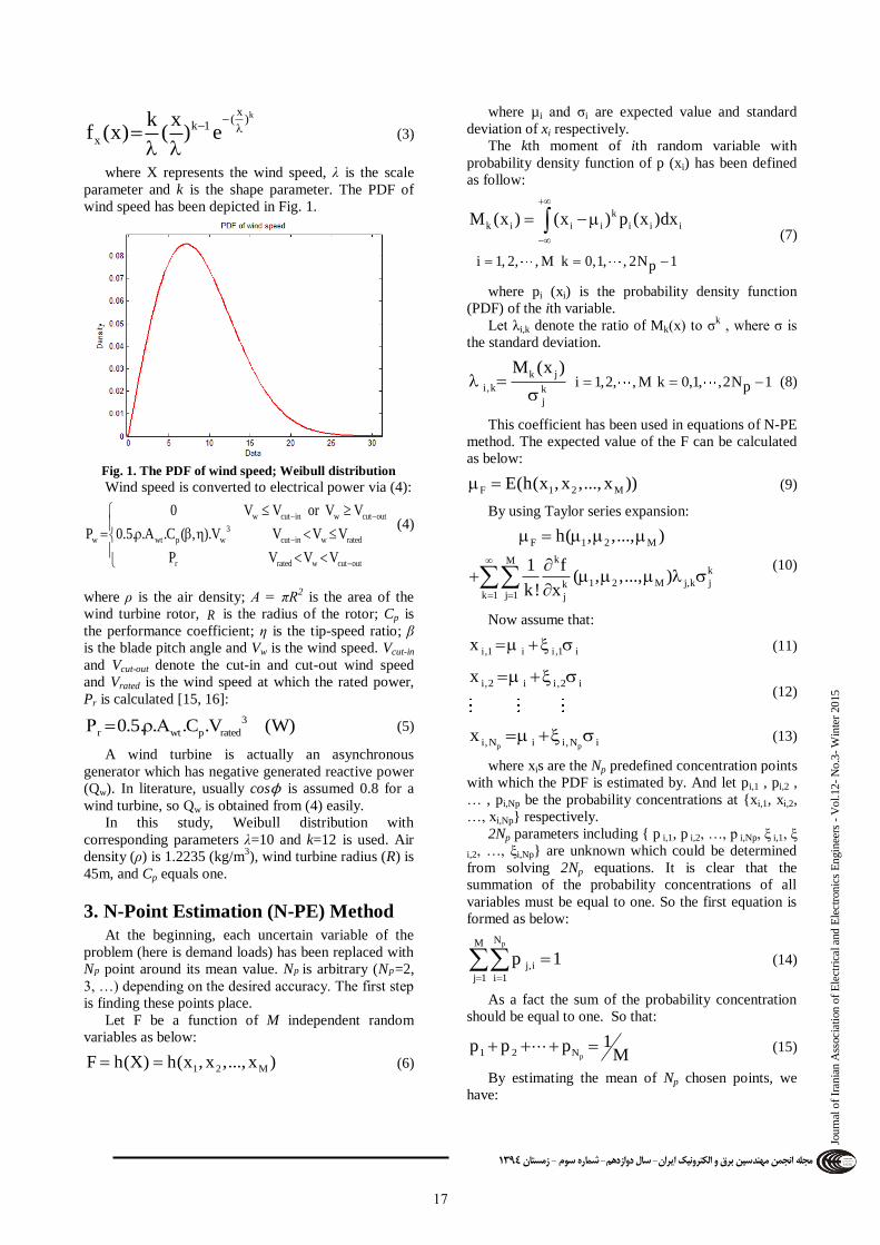
where X represents the wind speed, λ is the scale

parameter and k is the shape parameter. The PDF of

wind speed has been depicted in Fig. 1.

Fig. 1. The PDF of wind speed; Weibull distribution

Wind speed is converted to electrical power via (4):

w cut in w cut out

3

w wt p w cut in w rated

r rated w cut out

0 V V or V V

P 0.5. .A .C ( , ).V V V V

P V V V

(4)

where ρ is the air density; A = πR2 is the area of the

wind turbine rotor, R is the radius of the rotor; Cp is

the performance coefficient; η is the tip-speed ratio; β

is the blade pitch angle and Vw is the wind speed. Vcut-in

and Vcut-out denote the cut-in and cut-out wind speed

and Vrated is the wind speed at which the rated power,

Pr is calculated [15, 16]:

3

r wt p rated0.5. . .C .V (W) (5)

A wind turbine is actually an asynchronous

generator which has negative generated reactive power

(Qw). In literature, usually cosϕ is assumed 0.8 for a

wind turbine, so Qw is obtained from (4) easily.

In this study, Weibull distribution with

corresponding parameters λ=10 and k=12 is used. Air

density (ρ) is 1.2235 (kg/m3), wind turbine radius (R) is

45m, and Cp equals one.

3. N-Point Estimation (N-PE) Method

At the beginning, each uncertain variable of the

problem (here is demand loads) has been replaced with

NRpR point around its mean value. NRpR is arbitrary (NRpR=2,

3, …) depending on the desired accuracy. The first step

is finding these points place.

Let F be a function of M independent random

variables as below:

1 2 MF h(X) h(x , x ,..., x ) (6)

where µi and σi are expected value and standard

deviation of xi respectively.

The kth moment of ith random variable with

probability density function of p (xi) has been defined

as follow:

k

k i i i i i i

i 1, 2, , M k 0,1, , 2N 1p

M (x ) (x ) p (x )dx

(7)

where pi (xi) is the probability density function

(PDF) of the ith variable.

Let λi,k denote the ratio of Mk(x) to σk , where σ is

the standard deviation.

k j

i,k k

j

i 1,2, , M k 0,1, ,2N 1p

M (x )

(8)

This coefficient has been used in equations of N-PE

method. The expected value of the F can be calculated

as below:

F 1 2 ME(h(x , x ,..., x )) (9)

By using Taylor series expansion:

F 1 2 M

kMk

1 2 M j,k jkk 1 j 1 j

h( , ,..., )

1 f( , ,..., )

k! x

(10)

Now assume that:

i,1 i i ,1 ix (11)

i,2 i i,2 ix (12)

p pi,N i i,N ix (13)

where xis are the Np predefined concentration points

with which the PDF is estimated by. And let pi,1 , pi,2 ,

… , pi,Np be the probability concentrations at {xi,1, xi,2,

…, xi,Np} respectively.

2Np parameters including { p i,1, p i,2, …, p i,Np, ξ i,1, ξ

i,2, …, ξi,Np} are unknown which could be determined

from solving 2Np equations. It is clear that the

summation of the probability concentrations of all

variables must be equal to one. So the first equation is

formed as below:

pNM

j,i

j 1 i 1

p 1

(14)

As a fact the sum of the probability concentration

should be equal to one. So that:

p1 2 N1p p p

M (15)

By estimating the mean of Np chosen points, we

have:

17

دسي جوي ه يک ايراىهجل ا ن -ي برق الکتر -سال دازد 3194زهستاى - سمشوار

Journ

al of Iran

ian A

ssociatio

n o

f Electrical an

d E

lectronics E

ngin

eers - Vol.1

2- N

o.3

- Win

ter 2015

p

p

NM

F 1 2 M j,i

j 1 i 1

kMk k k

1 2 M j,1 j,1 j,N j,n jkk 1 j 1 j

f ( , ,..., ). p

1 f( , ,..., )(p . p . )

k! x

(16)

Make the first 2Np orders of (10) and (16)

equivalent, so we will find the 2Np-1 required

equations for jth variable as follow:

i i i

j,1 j,1 j,2 j,2 j,N j,N ip p

i 1, ,2N 1 j 1,2, ,Mp

p . p . p .

(17)

At the end we have a set of equation including (15)

and (17) in dimension of 2Np with 2Np unknowns

including { pi,1, pi,2, …, p i,Np, ξ i,1, ξ i,2, …, ξ i,Np} for

each variable of the system.

As (17) shows, 2Np-1 equations in the system are

nonlinear. Therefore, numerical techniques are required

to solve this set of equations. In this paper, this set of

equations has been solved using FSOLVE command of

MATLAB.

4. Application of N-PE Method to Solve

POFP

The following flowchart given by Fig. 2 explains how

the algorithm is performed:

Step 1: In the OPF problem, the random variables

are active power loads (PRDR) and reactive power loads

(QRDR). These variables which have been characterized

by probability density function (PDF) are considered as

inputs. Besides that, NRpR (number of estimated points) is

an input.

Step 2: For the zth random variable the set of

equations including (15), (17) has been solved to find

unknowns pz, j, ξz, j (j=1, 2… Np). After that, {xz,1, xz,2,

…, xz,Np} have been determined using (13).

Step 3: In this step, x z has been replaced with x z,j

and other random variables are kept at their mean

values to use them in deterministic OPF. OPF has been

run by means of MATPOWER, using this new value

for the zth variable and the mean values for other

variables. The results have been saved as below:

z,1 1 2 z,1 Mh ( , , , x , , ) (18)

z,2 1 2 z,2 Mh ( , , , x , , ) (19)

p pz,N 1 2 z,N Mh( , , ,x , , ) (20)

where θz is the result of deterministic OPF solution,

such as active generated power (PG) and reactive

generated power (QG) of the generators of the system.

Step 4: At the end, the final answer has been

obtained as below:

p p

M

i,1 i,1 i,2 i,2 i,N i,N

i 1

E(F) [p . p . p ]

(21)

p p

M2 2 2

i,1 i,1 i,2 i,2 i,N i,N

i 1

2

VAR(F) {p .[ ] p .[ ] p [ ] }

[E(F)]

(22)

where E(F) and VAR(F) are the mean value and the

variance of the specific output results respectively.

Start

· M random

variables

· Np

· z=1

z > M

· Solve equation set (13), (15) and

obtain {p z,1, p z,2, …, p z,Np, ξ z,1, ξ z,2,

…, ξz,Np}.

· Calculate {xz,1, xz,2, …, xz,Np}

· j=1

· Replace x z with x z,j and keep other

random variables at their mean

value.

· Run OPF using these values.

· Save the results as θz,j

· j=j+1

j > Np

No

z=z+1Yes No

Calculate final

result

Yes

Step 1

Step 2

Step3

Step 4

Fig. 2. Flowchart of proposed algorithm

5. Simulation Results

In order to demonstrate the effectiveness of the

proposed algorithm, it has been applied to IEEE 14-

Bus test case power system [17]. This system contains

14 buses, two generators, three synchronous

condensers (bus 3, 6, and 8), 10 load points, and 20

branches. The single line diagram of the system has

been depicted in Fig. 3.

18

Journ

al o

f Ir

ania

n A

ssoci

atio

n o

f E

lect

rica

l an

d E

lect

ronic

s E

ngin

eers

- V

ol.

12-

No.3

- W

inte

r 2015

دسي جوي ه يک ايراىهجل ا الکتر ن -ي برق ازد سم -سال د 3194زهستاى -شوار

Fig. 3. IEEE 14-Bus system

The cost function of each generator has been considered as (1) and the value of α, β, and γ which are constant coefficients has been presented in Table 1. In order to run OPF, some constraints such as maximum and minimum active and reactive power have been considered for each generation unit. These constraints have given in Table 2. Bus voltages could vary from 0.94 to 1.06 per unit. For all the transmission lines, long term rating has been considered equal to 9900 MVA.

Three different types of PDF have been considered for load points in this study; Normal, Uniform, and Weibull. A wind turbine with specifications which have been mentioned in Section 2 has been considered on Bus#11. Characteristic parameters of each PDF have been given in Table 3. Probability density functions of loads have been listed in Table 4.

Optimal power flow has been run in this system

using Monte Carlo (MC) simulation, Two Point

Estimation (T-PE) method, and Three Point Estimation

method. Final outputs are mean value and standard

deviation of active and reactive generated power of

each generator and synchronous condenser of the

system.

The stochastic OPF has been run using MC

simulation with 1500 simulations, T-PE method, and

Three Point Estimation method. The results of these

simulations have been given in Table 5, Table 6, and

Table 7 respectively. It can be seen that the results are

very close to each other, in spite of large differences in

required calculation time for each method. The

required calculation time for MC simulation, T-PE

method, and Three Point Estimation method have been

compared in Table 8.

Table. 2. Generators constraints (MW & MVAr)

Pmin Pmax Qmin Qmax Generator

0 332.4 0 10 G1

0 140 -40 50 G2

0 100 0 40 G3

0 100 -6 24 G4

0 100 -6 24 G5

Table. 1. Cost function coefficients

γ β α Generator

0.04303 20 0 G1

0.2500 20 0 G2

0.0100 40 0 G3

0.0100 40 0 G4

0.0100 40 0 G5

Table. 4. Probability density functions of loads

Bus Number

& Load Type

Distributio

n Type

First

Parameter(M

W)

Second

Parameter(M

W)

2 P Uniform 20 23.4

Q Uniform 10 15.4

3 P Uniform 90 98.4

Q Uniform 16 22

4 P Normal 47.8 2.25

Q Normal -3.9 1

5 P Normal 7.6 1.12

Q Normal 1.6 1

6 P Weibull 11.44 25

Q Weibull 8.17 5

9 P Normal 29.5 1.5

Q Normal 16.6 0.85

10 P Weibull 9.56 8

Q Weibull 6.32 5

12 P Uniform 5 7.2

Q Uniform 1 2.2

13 P Normal 13.5 0.7

Q Normal 5.8 1.3

14 P Uniform 13 16.8

Q Uniform 3 7

Table. 3. Characteristic parameters

PDF Type First Parameter Second Parameter

Normal Mean (µ) Variance (σ2)

Uniform Lower Bound (a) Upper Bound (b)

Weibull Scale Parameter (a) Shape Parameter

(b)

19

دسي جوي ه يک ايراىهجل ا ن -ي برق الکتر -سال دازد 3194زهستاى - سمشوار

Journ

al of Iran

ian A

ssociatio

n o

f Electrical an

d E

lectronics E

ngin

eers - Vol.1

2- N

o.3

- Win

ter 2015

The relative errors of active generated powers of

generators between MC simulation, T-PE method, and

Three Point Estimation method have been given in

Table 7. There are two considerable errors in Table 9,

19.38% and 21.76%.

It is because of the errors in numerical solution of a

nonlinear set of equations, including (17). However,

the errors are acceptable.

6. Conclusion

This paper presents N-Point estimation method to

handle stochastic smart grid’s problems such as,

probabilistic optimal power flow in presence of wind

generation. The proposed method has been tested on

the IEEE 14-bus system with an additional wind

turbine, in which the Monte Carlo method has been

used to compare the results with the two point and

three point estimation method. Results confirm very

good performance of T-PE method in terms of the

accuracy and calculation time. However, results show a

few considerable errors in T-PE method and Three

Point Estimation method; it is because of the error in

numeric solution of a nonlinear set of equations in

dimension of six. More advanced and accurate

techniques of numeric solution which requires

additional investigations can decrease these errors.

References [1] E. Santacana, G. Rackliffe, Le Tang and Xiaoming

Feng, “Getting Smart”, Power and Energy Magazine,

IEEE , Vol. 8, No. 2, March-April 2010, pp.41-48. [2] K. Moslehi and R. Kumar, “A Reliability Perspective

of the Smart Grid”, Smart Grid, IEEE Transactions on,

Vol.1, No.1, June 2010, pp. 57-64.

[3] A. Ipakchi and F. Albuyeh, “Grid of the future”, Power and Energy Magazine, IEEE, Vol.7, No.2, March-April

2009, pp.52-62.

[4] Chen Wang, Libao Shi, Liangzhong Yao, Liming

Wang, Yixin Ni, and Masoud Bazargan, “Modelling Analysis in Power System Small Signal Stability

Considering Uncertainty of Wind Generation,” Power

and Energy Society General Meeting, 2010 IEEE,

2010, pp. 1-7. [5] Xue Li, Yuzeng Li, and Shaohua Zhang, “Analysis of

Probabilistic Optimal Power Flow Taking Account of

the Variation of Load Power,” IEEE Trans. Power

Syst., vol. 23, no. 3, pp. 992-999, AUGUST 2008. [6] M. Madrigal, K. Ponnambalam, and V. H. Quintana,

“Probabilistic optimal power flow”, in Proc. IEEE

Can. Conf. Electrical and Computer Engineering,

Waterloo, ON, Canada, May 1998, pp. 385–388. [7] A. Schellenberg, W. Rosehart, and J. Aguado,

“Cumulant based probabilistic optimal power flow (P-

OPF) with Gaussian and gamma distributions,”, IEEE

Trans. Power Syst., vol. 20, no. 2, pp. 773-781, MAY 2005.

Table. 8. MCS, T-PEM, and 3-PEM Comparison

Simulation Type Calculation Time (s)

Monte Carlo 239.91

2-Point Estimation 9.45

3-Point Estimation 38.74

Table. 7. Results of Three Point Estimation method Gen.

&Cond.

Bus #

PG(Mean

Value)

PG(Standard

Deviation)

QG(Mean

Value)

QG(Standard

Deviation)

1 193.6502 6.4624 0.00069 0.00015

2 36.3789 1.7881 23.3024 2.1667

3 26.4201 2.3422 23.9568 2.1116

6 0.2704 0.00013 12.1941 2.5390

8 5.9960 1.9214 8.4142 0.6794

Table. 6. Results of T-PE method Gen.

&Cond.

Bus #

PG(Mean

Value)

PG(Standard

Deviation)

QG(Mean

Value)

QG(Standard

Deviation)

1 193.3617 1.4375 0.2376 0.00084

2 36.5462 0.2647 23.9595 1.8354

3 26.9418 1.9026 24.3729 1.7552

6 0.2786 1.8593 11.2044 2.4781

8 6.1192 2.0130 8.2872 0.5505

Table. 9. Relative errors of PG

Bus Number MCS , 2-PEM MCS , 3-PEM

1 0.2800 % 0.1313 %

2 0.2600 % 0.7180 %

3 0.7685 % 0.0408 %

6 19.3800 % 21.7590 %

8 1.8289 % 3.8054 %

Table. 5. Results of MC simulation (1500 simulations) Gen.

&Cond.

Bus #

PG(Mean

Value)

PG(Standard

Deviation)

QG(Mean

Value)

QG(Standard

Deviation)

1 193.9048 0.4429 0.2451 0.00085

2 36.6420 0.0852 23.4923 1.8523

3 27.1500 1.9669 24.0864 1.7263

6 0.3456 0.00077 9.8029 2.3874

8 6.2332 2.3037 8.0012 0.5301

20

Journ

al o

f Ir

ania

n A

ssoci

atio

n o

f E

lect

rica

l an

d E

lect

ronic

s E

ngin

eers

- V

ol.

12-

No.3

- W

inte

r 2015

دسي جوي ه يک ايراىهجل ا الکتر ن -ي برق ازد سم -سال د 3194زهستاى -شوار

[8] G. Verbiˇc and C. A. Cañizares, “Probabilistic optimal

power flow in electricity markets based on a two-point

estimate method,” IEEE Trans. Power Syst., vol. 21,

no. 4, pp. 1883–1893, Nov. 2006. [9] C.-L. Su, “Probabilistic load-flow computation using

point estimate method,” IEEE Trans. Power Syst., vol.

20, no. 4, pp. 1843–1851, Nov.2005.

[10] Juan. M. Morales and Juan. Pérez-Ruiz, “Point Estimate Schemes to Solve the Probabilistic Power

Flow,” IEEE Trans. Power Syst., vol. 22, no. 4, Nov.

2007.

[11] X. Liu and J. Zhong, “Point Estimate Method for Probabilistic Optimal Power Flow with Wind

Generation,”The International Conference on

Electrical Engineering, 2009.

[12] E. Rosenblueth, “Two-point Estimates In Probabilities,” Appl. Math. Modelling, vol. 5, Oct.

1981.

[13] B. Borkowska, “Probabilistic load flow,” IEEE Trans.

Power App. Syst.,vol. PAS-93, pp. 752–759, Apr. 1974.

[14] A. Schellenberg, W. Rosehart, and J. Aguado,

“Cumulant based probabilistic optimal power flow (P-

OPF),” in Proc. Int. Conf. Probabilistic Methods Applied Power Systems, Sep. 2004, pp. 506–511.

[15] P. Ramirez, J. A. Carta, “Influence of the data

sampling interval in the estimation of the parameter of

the Weibull wind speed probability distribution: a case study,” Energy Conv. Manag., Elsevier, vol. 46, pp.

2419-2438, 2005.

[16] T. Ackerman, “Wind Power in Power Systems,” Wiley,

2005. [17] R. Christie, UW Power System Test Case Archive,

Available:

http://www.ee.washington.edu/research/pstca/.

سيذحميذ فتحي ، مرتضي محمذی اردبلي، محمذعلي فتبحي [81]

مسمبن اورشی ذيتل ستميدر س ىيوقط كبری ب هييتع “اردكبوي

بب استفبد از یيگرمب ريب مرا مخسن رخ یيگرمب ي يکیالکتر

، 6جلذ ، ایران الکتريويک ي برقوشری مىذسي ، ”کيشوت تمیالگر

.8811، ببر ي تببستبن 8شمبر

حل مسئل پخش ببر بيى در "، احسبن افضالن،محمد جرابيبن [81]

گري ررات يبيترك تمیبب استفبد از الگر یورمبل ي اضطرار طیشرا

، الکتريويک ایران ي برقوشری مىذسي ، "، (PSO-NM) ذيي ولذر م

.8811، ببر ي تببستبن 8، شمبر 81جلذ

21