Probabilistic Martingales and BPTIME Classes

Kenneth W. Regan∗

State Univ. of N.Y. at BuffaloD. Sivakumar†

University of Houston

March 1998

Abstract

We defineprobabilistic martingalesbased on randomized approximationschemes, and show that the resulting notion ofprobabilistic measurehas sev-eral desirable robustness properties. Probabilistic martingales can simulatethe “betting games” of [BMR+98], and can cover the same class that a “nat-ural proof” diagonalizes against, as implicitly already shown in [RSC95].The notion would become a full-fledged measure on bounded-error com-plexity classes such asBPP and BPE if it could be shown to satisfy the“measure conservation” axiom of [Lut92] for these classes. We give a suffi-cient condition in terms of simulation by “decisive” probabilistic martingalesthat implies not only measure conservation, but also a much tighter boundederror probabilistic time hierarchy than is currently known. In particular itimplies BPTIME[O(n)] 6= BPP, which would stand in contrast to recentclaims of an oracleA giving BPTIMEA[O(n)] = BPPA. This paper alsomakes new contributions to the problem of defining measure onP and othersub-exponential classes. Probabilistic martingales are demonstrably strongerthan deterministic martingales in the sub-exponential case.

1 Introduction

Lutz’s theory of resource-bounded measure [Lut92] is commonly based onmartin-galesdefined on strings. A martingale can be understood as a gambling strategyfor betting on a sequence of events—in this case, the events are membership and∗Supported in part by National Science Foundation Grant CCR-9409104. Address for correspon-

dence: Computer Science Department, 226 Bell Hall, UB North Campus, Buffalo, NY 14260-2000.Email: regan@cs.buffalo.edu†Research initiated while the author was at SUNY/Buffalo, supported in part by National Science

Foundation Grant CCR-9409104. Email:siva@cs.uh.edu

non-membership of strings in a certain language. If the strategy yields unboundedprofit on a languageA, then it is said tocoverA, and the class of languages coveredhas measure zeroin a corresponding appropriate sense.

It is natural to ask whether gambling strategies can be improved, in the senseof covering more languages, if the gambler is allowed to randomize his bets. Ran-domized playing strategies are crucial in areas such as game theory, and proba-bilistic computation is believed or known to be more powerful than deterministiccomputation in various computational settings. Is this so in the setting of resource-bounded measure? We defineprobabilistic martingalesprecisely in order to studythis, basing them on the important prior notion of afully polynomial randomizedapproximation scheme(FPRAS) [KL83, JVV86, JS89].

Probabilistic martingales have already appeared implicitly in recent work. Forevery “natural proof”Π (see [RR97]) of sufficient density, there is a probabilisticmartingaled of equivalent complexity that covers the class of languages thatΠis useful against [RSC95]. The “betting games” of Buhrman et al. [BMR+98]can be simulated by probabilistic martingales of equivalent time complexity, asessentially shown by Section 5 of that paper. Hence in particular, probabilisticmartingales of2O(n) time complexity (which equals polynomial time in Lutz’snotation withN = 2n as the input length) can cover the class of languages thatare polynomial-time Turing-complete forEXP. This class is not known to becovered by any2n

O(1)-time deterministic martingale—and if so, thenBPP 6= EXP

[AS94, BFT95]. The ultimate point of our work here, however, is that probabilisticmartingales provide a new way to study general randomized computation.

For the study of sub-exponential time bounds, we lay groundwork by offering anew extension of Lutz’s measure theory to classes belowE. Our extension is basedon “lex-limited betting games” as defined in [BMR+98]. For measure onP it isweaker than some other notions that have been proposed in [AS94, AS95, Str97,CSS97], but it satisfies all of Lutz’s measure axioms (except for some “fine print”about infinite unions), and carries over desirable results and properties of Lutz’stheory fromE andEXP down to classes below. It also still suffices for the mainresult of [AS94].

We prove that a classC is covered by a probabilistic martingale of time com-plexity T (n) if and only if (unrelativized)C has DTIMEA[T (n)] measure zerorelative to a random oracleA. Hence in particular theEXP-complete sets haveEA-measure zero (orp-measure zero relative toA in Lutz’s terms), for a randomA. Our theorem is roughly analogous to the theorem thatBPP equals the class oflanguages that belong toPA for a randomA [BG81a, Amb86]. Hence we regardour notion as the best candidate for defining a measure on bounded-error classes

such asBPP, BPE, andBPEXP. The latter two classes are defined from thegeneral definition:

Definition 1.1. A languageL belongs toBPTIME[t(n)] if there is a probabilisticTuring machineM running in timet(n) such that for all inputsx, Pr[M(x) 6=L(x)] < 1/3.

If t belongs to a family of time bounds that is closed under multiplication byn,then standard “repeated trials” amplification can be used to reduce the error proba-bility 1/3 below1/2n on inputs of lengthn. Hence the definitions ofBPP, BPE,andBPEXP are robust, but whether the error probability can be reduced in theresulting definition ofBPTIME[O(nk)] for fixed k is pertinent to open problemsin this paper.

The nub is whether our candidate for probabilistic measure has the crucial“measure conservation” property, i.e. whether one can show thatBPP doesnothave “BPP–measure zero,” or thatBPE does not have probabilisticE-measurezero, and so on. We give a sufficient condition that is natural and reasonably plausi-ble, namely that every probabilistic martingaled can be simulated by a probabilisticmartingaled′ (in the sense ofd′ succeeding on all languages thatd succeeds on andhaving a randomized approximation scheme of similar time complexity) such thatevery change in the value ofd′ is not negligibly close to zero. For deterministicmartingales this is an easy simulation. If this holds for probabilistic martingales,then measure conservation holds, and they really define a measure.

Since we show thatBPTIME[O(n)] is covered by aBPP-martingale, andBPP by a probabilistic quasi-polynomial time martingale, andBPE by aBPEXPmartingale (and so on), this would have the following consequence:

BPTIME[O(n)] ⊂ BPP ⊂ BP[qpoly ] ⊂ . . .⊂ BPE ⊂ BPEXP.

None of these successive inclusions is known to be proper. Indeed, Rettinger andVerbeek [RV97] claim to have an oracleA relative to whichBPTIMEA[O(n)] =BPPA = BPTIMEA[qpoly ] (hence alsoBPEA = BPEXPA by translation),fixing a flawed result of Fortnow and Sipser [FS89, FS97]. Thus our simulationproblem ties in to the important open question of whether bounded-error proba-bilistic time enjoys a tight time hierarchy like that of deterministic time. We pro-pose to turn this question on its head by analyzing the problem for probabilisticmartingales, which is equivalent to a more-general problem about randomized ap-proximation schemes treated in [CLL+95]. For instance, it may be useful to seekand study oraclesA relative to which some probabilistic martingale has no decisivesimulation, independent of whether the oracle claim of [RV97] holds up.

2 Resource-Bounded Measure

A martingaleis explicitly defined as a functiond from 0, 1 ∗ into the nonnegativereals that satisfies the following “exact average law”: for allw ∈ 0, 1 ∗,

d(w) =d(w0) + d(w1)

2. (1)

The interpretation in Lutz’s theory is that a stringw ∈ 0, 1 ∗ stands foran initial segment of a language over an arbitrary alphabetΣ as follows: Lets1, s2, s3, . . . be the standard lexicographic ordering ofΣ∗. Then for any languageA ⊆ Σ∗, writew v A if for all i, 1 ≤ i ≤ |w|, si ∈ A iff the ith bit ofw is a 1. Wealso regardw as a function withdomain s1, . . . , s|w| and range 0, 1 , writingw(si) for theith bit ofw. A martingaled succeeds ona languageA if the sequenceof valuesd(w) for w v A is unbounded. LetS∞[d] stand for the (possibly empty,often uncountable) class of languages on whichd succeeds.

Definition 2.1 ([Lut92]). Let ∆ be a complexity class of functions. A classCof languageshas∆-measure zero, writtenµ∆(C) = 0, if there is a martingaledcomputable in∆ such thatC ⊆ S∞[d]. One also says thatd coversC.

Lutz defined complexity bounds in terms of the length of the argumentw to d,which we denote byN . However, we also work in terms of the largest lengthn ofa string in the domain ofw. ForN > 0, n equalsblogNc; all we care about isthatn = Θ(logN) andN = 2Θ(n). Because complexity bounds on languages wewant to analyze will naturally be stated in terms ofn, we generally prefer to usenfor martingale complexity bounds. The following correspondence is helpful:

Lutz’s “p” ∼ NO(1) = 2O(n) ∼ µE

Lutz’s “p2” ∼ 2(logN)O(1)= 2n

O(1) ∼ µEXP

One effect of the change is that the function class∆ corresponding to a time-bounded complexity classD is clear—one simply uses the same time bound forfunctions. We carry forward Lutz’s usage of saying that a classC has measure zeroin a classD if µD(C ∩D) = 0, andmeasure one inD if D \ C has measure zero inD.

The desire to extend Lutz’s theory to define measures on classesD below Eruns into well-known technical problems. We will later propose a new definitionthat works well across the board for all families of sub-exponential time boundsthat are closed under squaring, and is equivalent to Lutz’s for bounds atE andabove. However, we prefer to introduce probabilistic martingales in the specificcase ofE-measure and defer the more-general results to later sections.

3 Measure on E via Probabilistic Computations

Our first definition of measure via probabilistic computations has the followingbasic idea. Lutz’s adaptation of classical measure theory to complexity classesis based onreal-valued martingale functions. To turn this into a meaningfulcomplexity-based notion, Lutz appeals to Turing’s notion of computing a real num-ber by arbitrarily close dyadic rational approximations (see [Ko83]). In a similarvein, we would like to define probabilistic measure via martingales that can beef-ficiently computed probabilistically to arbitrary accuracy. Among many possiblenotions of probabilistic computation of numerical functions, the following naturaldefinition due to Karp and Luby [KL83] has risen to prominence.

Definition 3.1. A functionf : Σ∗ → Q≥0 has afully polynomial-time randomizedapproximation scheme(FPRAS) if there are a probabilistic Turing machineM anda polynomialp such that for allx ∈ Σ∗ andε, δ ∈ Q>0,

Pr[(1− ε)f(x) ≤M(x, ε, δ) ≤ (1 + ε)f(x)] ≥ 1− δ, (2)

andM(x, ε, δ) halts withinp(|x|+ (1/ε) + log(1/δ)) steps.

(It is equivalent to removeδ and write “1− ε” on the right-hand side of (2), but theabove form is most helpful to us.)

Definition 3.2. A probabilisticE-martingaleis a martingale that has an FPRAS.

This definition bounds the time to approximate martingale valuesd(w) by a poly-nomial inN = |w|, which is the same aspoly(2n) = 2O(n). Our later generaliza-tion of an FPRAS will work nicely for all time bounds, stated in terms ofn.

Now to obtain a notion of probabilisticE-measure, we simply carry over Defi-nition 2.1.

Definition 3.3. A classC of languageshas probabilisticE-measure zero, writtenµBPE(C) = 0, if there is a probabilisticE-martingaled such thatC ⊆ S∞[d].

A viewpoint orthogonal to randomized approximation arises naturally fromclassical measure theory.

Definition 3.4. A “randomized martingale machine”M has access to an infinitesequenceρ ∈ 0, 1ω, which it uses as a source of random bits. Every fixedρdefines a martingaledρM , and for any inputw, M first computesdρM (v) on thesuccessive prefixesv < w before computingdρM (w), drawing successive bits fromρ without repetition.M runs inE-time if this computation takes time2O(n) =poly(|w|).

Now we want to say that a classC has probabilistic measure zero if a “random”ρ makesdρM coverC. To do this, we simply use the long-established definition of“random” via classical Lebesgue measureon the space 0, 1 ω of sequencesρ,which is much the same as the familiar Lebesgue measure on the real numbers in[0, 1].

Definition 3.5. A classC is “E-random-null” if there is anE-time randomizedmartingale machineM such that for allA ∈ C, the set

ρ : A ∈ S∞[dρM ]

has Lebesgue measure one.

For countable classesC, it is equivalent to stipulate that the set ofρ such thatC ⊆ S∞[dρM ] has Lebesgue measure one. In the case of uncountable classes suchasP/poly , however, we do not know such an equivalence. Nevertheless, Defini-tion 3.5 is equivalent to Definition 3.3, and to a third condition stated familiarly interms of “random oracles,” which differ from random sequencesρ in that bits canbe used with repetitions. Note thatC is unrelativized in the third case.

Theorem 3.1 For any classC of languages, the following statements are equiva-lent.

(a) There is a probabilisticE-martingale that coversC.

(b) C is E-random-null.

(c) For a random oracleA, C hasEA-measure zero.

The neat thing about the equivalence is that Definition 3.3 allows us to treat a“probabilistic martingale” as a single entity rather than the ensemble of Defini-tion 3.5, while Definition 3.5 does not involve an approximation parameterε, andmakes no reference to bounded-error computation at all! With this understood, wecan point out that probabilisticE-martingales have already implicitly been used inthe literature. The construction in Theorem 18 of [RSC95] shows that for every“natural proof/property”Π of sufficient density, there is a probabilistic martingaleof equivalent complexity that covers the class of languages thatΠ is useful against.The constructions in Section 5 of [BMR+98] show that every “E-betting game”can be simulated by a probabilisticE-martingale. These two constructions hold forEXP in place ofE as well.

The proof of Theorem 3.1 is deferred until Section 6, where the generalizationto other time bounds is stated and proved. The proof is more informative in thegeneral setting. Its general workings are similar to the proofs by Bennett and Gill[BG81b] and Ambos-Spies [Amb86] thatBPP equals the class of languages thatbelong toPA for a random oracleA. These proofs extend to show thatBPE equalsthe class of languages that belong toEA for a random oracleA. The next sectionexplores how well our unified definitions serve as a notion of measure “on”BPE.

4 Measure Properties and BP Time Hierarchies

The important axioms for a measureµ on a complexity classD, as formulated byLutz [Lut92] and summarized in [AS94], are:

M1 Easy unions of null sets are null.We skirt the difficult formal definition ofan “easy” infinite union in [Lut92] and concentrate on the “finite unions”case: ifC1 andC2 are subclasses ofD with µ(C1) = 0 andµ(C2) = 0, thenµ(C1 ∪ C2) = 0.

M2 Singleton sets of easy languages are null.For all languagesL ∈ D,µ(L ) = 0.

M3 The whole space is not null.In other words, it is not the case thatµ(D) = 0.This is called “measure conservation” in [Lut92]. Under the stipulation thatfor C ⊆ D, µ(C) = 1 ⇐⇒ µ(D\C) = 0, this can be rewritten asµ(D) = 1.

All of the recent attempts to strengthen Lutz’s measure framework to make moreclasses null have missed out on one of these axioms, most notably finite unions[AS95, BMR+98], and this paper is no exception.

Why is it interesting to meet these axioms? A “pure” reason is that theyabstract out the distinguishing characteristics of Lebesgue measure, and meetingthem assures the integrity of a measure notion. They can also have direct connec-tion to open problems in complexity theory, however. A recent example is thatif the “betting-game measure” of [BMR+98] has the finite-unions propertyM1,then the nonrelativizable consequenceBPP 6= EXP follows. A similar inter-est applies here: We show that probabilistic martingales satisfyM1 andM2 withD = BPE. If they also satisfyM3, thentight BPTIME hierarchies follow—inparticular,BPTIME[O(n)] ⊂ BPP ⊂ BPTIME[qpoly(n)].

This consequence is interesting at this time because Rettinger and Ver-beek [RV97] have recently claimed to construct an oracleA relative to which

BPTIMEA[O(n)] = BPPA = BPTIMEA[qpoly(n)], which would fix the mainresult of Fortnow and Sipser ([FS89], withdrawn in [FS97]). We have not yet beenable to verify this claim, but the point is that bounded-error probabilistic time is notknown to have a tight hierarchy like that for deterministic or nondeterministic oreven unbounded-error probabilistic time. Karpinski and Verbeek [KV87] provedthatBPP, and alsoBPTIME[qpoly(n)] andBPTIME[t(n)] for some boundst(n)slightly above quasi-polynomial, are properly contained in∩ε>0BPTIME[2n

ε].

This result and its translates are basically the best ones known. Thus interest in ourwork partly depends on how well the following notion provides a new angle on theproblem of diagonalizing out of smallerBPTIME classes into larger ones.

Intuitively, a martingaled is decisiveif it never makes a bet so small that itswinning is insubstantial for the goal of succeeding on any language. In the presentcase of exponential time, supposed on stringsw of lengthN makes bets of mag-nitude less than1/N2. SinceΠN≥1(1 + 1/N2) < ∞, even ifall such bets winalong a languageA, d still does not succeed onA. Hence we would consider anyindividual bet of this size to be insubstantial. Our formal definition actually relaxesthe threshold from1/N2 to 1/Nk for any fixedk.

Definition 4.1. A (probabilistic)E-martingaled is decisiveif there existsk ≥ 1such that for allw, eitherd(w1)− d(w) = 0, or |d(w1)− d(w)| ≥ 1/|w|k.

Proposition 4.1 (a) ProbabilisticE-martingales satisfyM1 andM2.

(b) Decisive probabilisticE-martingales satisfyM2 andM3.

Proof. (a) Givend1 andd2 coveringC1 andC2, the functiond3 = (d1 + d2)/2coversC1 ∪ C2, and has a randomized approximation scheme of the same order ofrunning time and precision as those ford1 andd2. (Note thatd3 is the same asflipping a coin to decide whether to bet according tod1 or d2 on a given string.)For infinite unions, we defer the proof until Section 7.

For M2 in (a) and (b), given a fixed languageA ∈ BPE, use amplificationto find a probabilistic2O(n)-time TM MA such that for allx of any lengthn,Pr[MA(x) = A(x)] > 1− 1/2n

2. Now letd be the trivial martingale that doubles

its capital at every step alongA and gets wiped out to zero everywhere else. Thend is decisive. To compute an FPRAS ford(w), useMA to test for alli whetherwi = 1 ⇐⇒ si ∈ A. With high probability all the tests are correct, and so thevalue—either zero or2|w|—is correct with the same probability.

(b) For M3, given a decisive probabilisticE-martingaled, define a sequenceλ = w0 < w1 < w2 . . . inductively by

wi+1 = wi1 if d(wi1) < d(wi),

= wi0 otherwise.

This infinite sequence defines a languageA. Givenk from Definition 4.1, we canuse amplification to obtain anE-computable FPRASM for d such that for allw,Pr[|M(w) − d(w)| < 1/Nk+1] > 1 − 1/2n

2. (Recall thatN = 2n = |w|.) Now

defineMA to be a machine that on any inputx first runs itself recursively on allinputsy < x. The recursive calls build up a stringw whose domain is all thestrings up to but not includingx. Again with high probability,w = wN−1. Finally,MA computesM(w1) and compares it to its already-computed valueM(w). IfM(w1) < M(w),MA acceptsx; elseMA rejectsx.

The point is that owing to decisiveness, wheneverx ∈ A, |d(w1) − d(w)|is large enough that the approximating valuesM(w) and M(w1) will showM(w1) < M(w) with high probability, soMA will accept. Similarly wheneverx /∈ A, MA will most likely not getM(w1) < M(w), and with high probabilitywill correctly rejectx. SinceMA(x) does little more than run the FPRASM 2n

times,MA runs in2O(n) time, and soA ∈ BPE.

The construction in (a) fails to establishM1 for decisiveE-martingales. Theproblem is thatd1 andd2 can be decisive, but a valued1(w) can be positive andd2(w) negative such thatd1(w)− d2(w) is close to but different from zero. We donot know of any other strategy that makesM1 hold for decisive martingales, so thatthey would yield a fully-qualified notion of measure. Now do we know whetherM1 holding for them would have any larger-scale complexity consequences.

The “bigger game,” of course, is whether every probabilisticE-martingaledcan be simulated by a decisive oned′, in the sense thatS∞[d] ⊆ S∞[d′], fromwhich M3 would follow. For deterministicE-martingales this is a simple simula-tion: taked′ = (d+ e)/2, wheree bets an amount(1/2) · (1/N2) in the directionthat takes the combined bet away from zero. The particular probabilistic martin-galesd that we care about are those that arise in the proof of the next theorem.

Theorem 4.2 For all fixedc > 0, BPTIME[2cn] can be covered by a probabilisticE-martingale.

The tricky part of this, compared to the simple proof that DTIME[2cn] has mea-sure zero inE, is that it may not be possible to obtain a recursive enumerationof “BPTIME[...] machines.” However, probabilistic martingales (though maybenot decisive ones) can take up the slack of starting with a larger enumeration ofunbounded-errorprobabilistic TMs, and arrange to succeed on those TMs thathappen to have bounded error.

Proof. TakeP1, P2, . . . to be a standard recursive enumeration of probabilistic Tur-ing machines that run in time2cn. We define a “randomized martingale machine”M as follows.M divides its initial capitalC0 = 1 into infinitely many “shares”sk = 1/2k2 for k ≥ 0 (with an unused portion1 − π2/12 of C0 left over). Eachsharesk is assigned to the corresponding machinePk, maintains its own capital,and (for a fixed random inputρ) computes a martingale that bets a nonzero amountonly on stringsx of the formy10k. The martingale computed byM is well-definedby the sum of the shares.

To play sharesk on a stringx,M uses its random bits to simulatePk 2cn-manytimes, treating acceptance as+1 and rejection as−1, and letsν be the sample meanof the results. (OrM can apply the construction in [GZ97], which is defined forany probabilistic TM even though it only amplifies whenPk has bounded error.)M then bets a portionν/2 of the current capital of sharesk with the same sign asν. ThenM runs in timeO(22cn).

For anyPk that has bounded error probability, a measure-one set of randomsequences give:

• for all but finitely many0n ∈ L(Pk), ν > 1/2, and

• for all but finitely many0n /∈ L(Pk), ν < −1/2.

For any sequence in this set, sharesk survives a possible finite sequence of lossesand eventually grows to+∞. HenceM succeeds onL(Pk).

By our equivalence theorem, Theorem 3.1,M defines a probabilistic martin-galed that has an FPRAS. We may fail to obtain such ad that is decisive, however,for two main reasons. First and foremost, whenPk has unbounded error, the sam-ple meanν may be very close to zero. However, this does not preventan individualsharesk from playing a decisive betting strategys′k: if |ν| < 1/3 then bet zero.Other thresholds besides1/3 can be used, and can be varied for differentx, orscaled toward zero as1/|x|2, and so on. Since the shares play on different strings,the combination of the revised sharess′k yields a functiond′ that is decisive (i.e.,this is not the problem inM1 for decisive martingales). The second rub, however,is thatd′ may no longer be fully randomly approximable. This is because a tinydifference in a reportedν may cross the threshold and cause a displacement in thevalue ofd′ that is larger than the scheme allows. Put another way, the random vari-ableν for a particularxmay happen to be centered on the currently-used threshold,so that two widely-displaced values are output with roughly equal probability.

Seen in isolation, the problem of simulating a time-t(n) probabilistic martin-galed by a decisived′ is tantalizing. There seems to be slack for fiddling with

thresholds to defined′, or trying to take advantage of the fact that a martingalemust make infinitely many large bets along any language that it succeeds on. Orone could try to make one of the parts of the proof of Theorem 6.2 below producea decisive probabilistic martingale from the given one. However, this problem istied to (and basically a re-casting of) the longer-studied problem of diagonalizingagainst bounded-error probabilistic machines:

Theorem 4.3 If all probabilistic E-martingales can be simulated by decisive ones,then for allk > 0, BPTIME[nk] 6= BPP.

Proof. By Theorem 4.2, it immediately follows that for allc > 0,BPTIME[2cn] 6= BPE. The conclusion then follows by familiar “translation”or “padding” techniques.

Rather than rely on translation/padding results as in the proof of Theorem 4.3,however, we find it more informative to do the measure and diagonalization directlyon BPP. The next section makes this possible, and independently contributes tothe growing debate about the “proper” way to extend Lutz’s theory to measure onsub-exponential time classes.

5 A New Take on Sub-Exponential Measure

The key idea is to focus on the “betting strategy” that a martingale represents.The strategy plays on an unseen languageA, and tries to win money by “pre-dicting” the membership or non-membership of successive stringsx in A. Stan-dardly, a martingaled corresponds to the strategy that starts by betting the amountB1 = d(1) − d(λ) “on” the assertionλ ∈ A, and given a stringw that codes themembership of all stringsy < x in A, betsBx = d(w1) − d(w) on x. Here anegativeBx means that the bet wins ifx /∈ A. For measure atE and above, onecan freely switch between the two views because the (upper bound on the) timeto compute all ofd(λ), d(1), . . . , d(w) has the same order as the time to computed(w) alone.

For sub-exponential time bounds, however, one has to choose one’s view. Pre-vious proposals for measures on classes belowE [May94, AS94, AS95, Str97,CSS97] have worked directly with the martingales. We apply time bounds directlyto the betting strategies, relaxing the condition that they must bet onsuccessive

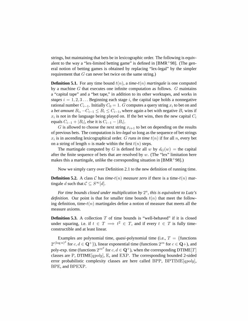
strings, but maintaining that bets be in lexicographic order. The following is equiv-alent to the way a “lex-limited betting game” is defined in [BMR+98]. (The gen-eral notion of betting games is obtained by replacing “lex-legal” by the simplerrequirement thatG can never bet twice on the same string.)

Definition 5.1. For any time boundt(n), a time-t(n) martingaleis one computedby a machineG that executes one infinite computation as follows.G maintainsa “capital tape” and a “bet tape,” in addition to its other worktapes, and works instagesi = 1, 2, 3 . . . Beginning each stagei, the capital tape holds a nonnegativerational numberCi−1. Initially C0 = 1. G computes a query stringxi to bet on andabet amountBi,−Ci−1 ≤ Bi ≤ Ci−1, where again a bet with negativeBi wins ifxi is not in the language being played on. If the bet wins, then the new capitalCiequalsCi−1 + |Bi|, else it isCi−1 − |Bi|.

G is allowed to choose the next stringxi+1 to bet on depending on the resultsof previous bets. The computation islex-legalso long as the sequence of bet stringsxi is in ascending lexicographical order.G runs in timet(n) if for all n, every beton a string of lengthn is made within the firstt(n) steps.

The martingale computed byG is defined for allw by dG(w) = the capitalafter the finite sequence of bets that are resolved byw. (The “lex” limitation heremakes this a martingale, unlike the corresponding situation in [BMR+98].)

Now we simply carry over Definition 2.1 to the new definition of running time.

Definition 5.2. A classC hastime-t(n) measure zeroif there is a time-t(n) mar-tingaled such thatC ⊆ S∞[d].

For time bounds closed under multiplication by2n, this is equivalent to Lutz’sdefinition. Our point is that for smaller time boundst(n) that meet the follow-ing definition, time-t(n) martingales define a notion of measure that meets all themeasure axioms.

Definition 5.3. A collection T of time bounds is “well-behaved” if it is closedunder squaring, i.e. ift ∈ T =⇒ t2 ∈ T , and if everyt ∈ T is fully time-constructible and at least linear.

Examples are polynomial time,quasi-polynomial time (i.e.,T = functions2c(logn)d for c, d ∈ Q+), linear exponential time (functions2cn for c ∈ Q+), andpoly-exp. time (functions2cn

dfor c, d ∈ Q+), when the corresponding DTIME[T ]

classes areP, DTIME[qpoly ], E, andEXP. The corresponding bounded 2-sidederror probabilistic complexity classes are here calledBPP, BPTIME[qpoly ],BPE, andBPEXP.

Proposition 5.1 For any well-behaved collectionT of time bounds, time-t(n) mar-tingales fort ∈ T define a measure onDTIME[T ] that meets measure axiomsM1–M3.

Proof. For the finite-union version ofM1, suppose we are givenG1 andG2 fromDefinition 5.1. DefineG3 to divide its initial capital into two equal “shares”s1

ands2, which follow the respective betting strategies used byG1 andG2. In con-trast to the situation for general betting games in [BMR+98], where closure underfinite unions impliesBPP 6= EXP, the point is that owing to the lex-order stipula-tion,G3 can play the two shares side-by-side with no conflicts. Whichever share’schoice of next string to bet on is the lesser gets to play next; if they both bet on astringx, thenG3’s bet is the algebraic sum of the two bets.

We postpone the definition and treatment of the infinite-unions case until theend of this section.

For M2, we actually show that for any time-t(n) martingaled, there is atime-t(n) printable languageA that is not covered byd. LetM start simulating theGfor d, and definex ∈ A iff G makes a negative bet onx. ThenM can print out allthe strings inA of length up ton within its first t(n) steps.

For M3, we show the stronger result that for anyt ∈ T , DTIME[t(n)] hastime-T measure zero. TakeP1, P2, P3, . . . to be a recursive presentation of time-t(n) Turing machines so that the language (i, x) : x ∈ L(Pi) can be recognizedby a machineM that runs in time, say,t(n)2. LetG divide its initial capital intoinfinitely many “shares”si, wheresi has initial capital1/2i2. To assure meetingthe time bound,G bets only on tally stringsx = 0j as follows: Leti be maximumsuch that2i dividesj. Then bet all of the current value of sharesi positively if x ∈L(Pi), negatively otherwise. For allA ∈ DTIME[t(n)], the sharesi correspondingto anyPi that acceptsA doubles its capital infinitely often, makingG succeed onA regardless of how the other shares do. ThenG runs in timeO(nt(n)2), whichbelongs toT .

Definition 5.1 defines a single infinite process that begins with empty input.We want an equivalent definition in terms of the more-familiar kind of machinethat has finite computations on given inputs. We use the same model of “randominput access” Turing machinesM used by others to define measures on classesbelowE [May94, AS94, AS95], but describe it a little differently: LetM have an“input-query” tape on which it can write a stringsi and receive the bitwi of w thatindexessi. Initially we place onM ’s actual input tape the lexically last stringxthat is indexed byw (if |w| = N , thenx = sN ), and writeM(w : x) orM(w : N)to represent this initial configuration.

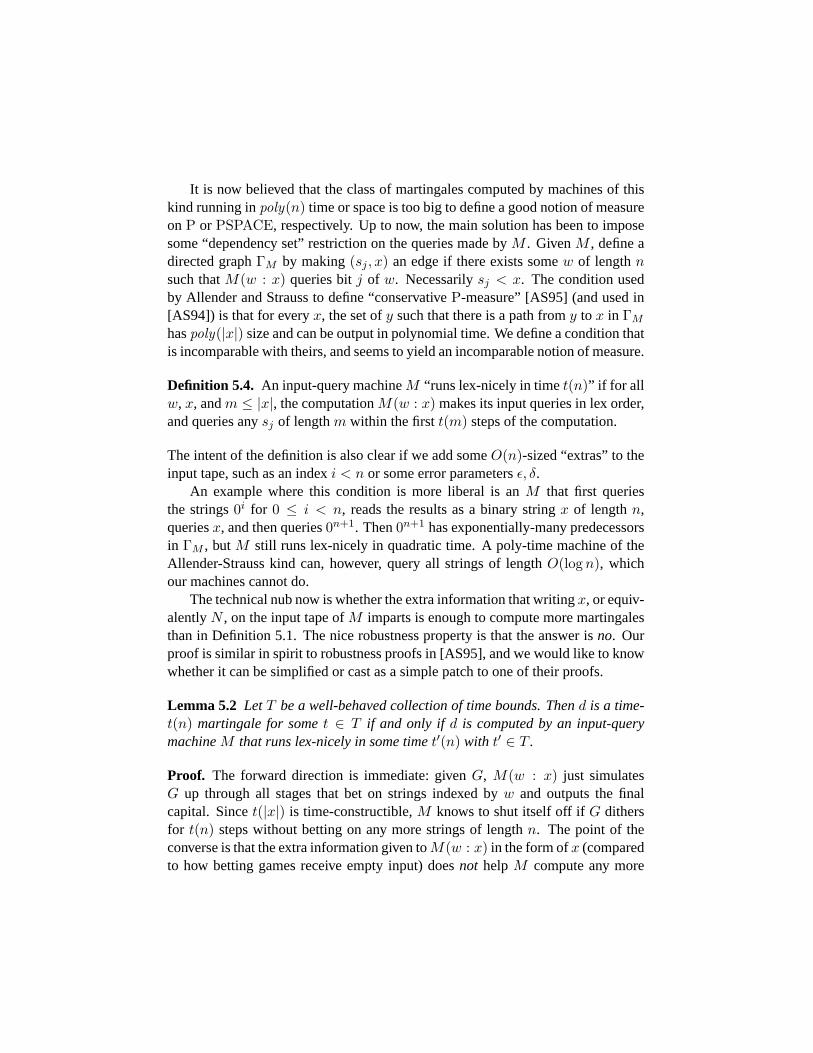
It is now believed that the class of martingales computed by machines of thiskind running inpoly(n) time or space is too big to define a good notion of measureon P or PSPACE, respectively. Up to now, the main solution has been to imposesome “dependency set” restriction on the queries made byM . GivenM , define adirected graphΓM by making(sj , x) an edge if there exists somew of lengthnsuch thatM(w : x) queries bitj of w. Necessarilysj < x. The condition usedby Allender and Strauss to define “conservativeP-measure” [AS95] (and used in[AS94]) is that for everyx, the set ofy such that there is a path fromy to x in ΓMhaspoly(|x|) size and can be output in polynomial time. We define a condition thatis incomparable with theirs, and seems to yield an incomparable notion of measure.

Definition 5.4. An input-query machineM “runs lex-nicely in timet(n)” if for allw, x, andm ≤ |x|, the computationM(w : x) makes its input queries in lex order,and queries anysj of lengthm within the firstt(m) steps of the computation.

The intent of the definition is also clear if we add someO(n)-sized “extras” to theinput tape, such as an indexi < n or some error parametersε, δ.

An example where this condition is more liberal is anM that first queriesthe strings0i for 0 ≤ i < n, reads the results as a binary stringx of lengthn,queriesx, and then queries0n+1. Then0n+1 has exponentially-many predecessorsin ΓM , butM still runs lex-nicely in quadratic time. A poly-time machine of theAllender-Strauss kind can, however, query all strings of lengthO(log n), whichour machines cannot do.

The technical nub now is whether the extra information that writingx, or equiv-alentlyN , on the input tape ofM imparts is enough to compute more martingalesthan in Definition 5.1. The nice robustness property is that the answer isno. Ourproof is similar in spirit to robustness proofs in [AS95], and we would like to knowwhether it can be simplified or cast as a simple patch to one of their proofs.

Lemma 5.2 LetT be a well-behaved collection of time bounds. Thend is a time-t(n) martingale for somet ∈ T if and only if d is computed by an input-querymachineM that runs lex-nicely in some timet′(n) with t′ ∈ T .

Proof. The forward direction is immediate: givenG, M(w : x) just simulatesG up through all stages that bet on strings indexed byw and outputs the finalcapital. Sincet(|x|) is time-constructible,M knows to shut itself off ifG dithersfor t(n) steps without betting on any more strings of lengthn. The point of theconverse is that the extra information given toM(w : x) in the form ofx (comparedto how betting games receive empty input) doesnot helpM compute any more

martingales. The effect is similar to the robustness results for the “conservative”measure-on-P notions of [AS95]. The main point is the following claim:

Claim 5.3 Supposev is a proper prefix ofw such thatd(v1) 6= d(v). ThenM(w :x) must query the stringyv indexed by the ‘1’ inv1.

To prove this, suppose not. TakeW = w′ : |w′| = |w| andv v w′ , W1 =w′ ∈ W : v1 v w′ , andW0 = W \W1. Thanks to the lex-order restriction,noneof thew′ ∈W causeM(w′ : x) to queryyv—they all make the same querieslexically less thanyv, and then either all halt with no further queries, or all makethe same query higher thanyv and can never queryyv from that point on. Now forall w1 ∈W1, there is a correspondingw0 ∈W0 that differs only in the bit indexingyv. It follows thatM(w1 : x) andM(w0 : x) have the same computation. But thenthe average ofM(w1 : x) overw1 ∈ W1 must equal the average ofM(w0 : x)overw0 ∈ W0, which contradictsd(v0) 6= d(v1) sinced is a martingale. Thisproves the claim.

It follows that if v is a shortest initial segment such thatd(v1) 6= d(v), thenfor everyw with |w| > |v|, the computationM(w : |w|) queriesyv, after perhapsquerying some strings lexically beforeyv. Then for a shortestv0 extendingv0with d(v01) 6= d(v0), and allw with |w| > |v0| andv0 v w, the computationM(w : |w|) must queryyv0 , and so on. . . and similarly forv1 extendingv1. . .

Now the lex-limited betting gameG simulatingM takes shape: For alln, thephase of the computation in whichG bets on some (or no) strings of lengthnbegins by simulatingM(w : 1t(n)). WheneverM(w : 1t(n)) queries a stringxof lengthn, call x a “top-level query.”G then simulatesM(w : x) in order tolearn what to bet onx. G maintains a table of all queries made byM and theirresults. If a stringy < x queried byM(w : x) is a top-level query, by the lex-orderrestriction applied toM(w : 1t(n)), y will already be in the table. Ify is not inthe table, thenG doesnot queryy—indeed, it might violate the runtime-provisoto queryy if y is short. Instead,G proceeds as though the answer toy is “no.”Finally, if M(w : x) queriesx, G simulates both the “yes” and “no” branches andtakes half the signed difference as its bet. (IfM(w : x) does not queryx, thenGbets zero onx.) By Claim 5.3, the average of the two branches is the same as thevalue ofM(w : x′) for the top-level queryx′ lexically precedingx (or the averageis d(λ) = 1 in casex is the first query). By induction (see next paragraph), thisequals the capitalG has at this stage, soG has sufficient capital to make the bet.ThenG queriesx. Whent(n) steps of the simulation ofM(w : 1t(n)) have goneby, or whenM(w : 1t(n)) wishes to query a string of length> n,G abruptly skipsto the next stage of simulatingM(w : 1t(n+1)) and handling any queries of lengthn+ 1 that it makes.

For correctness, it suffices to argue that the valuesG computes while simulatingM(w : x) always equalM(w : x), despite the possibly-different answers to non-top-level queriesy. Supposev andv′ be two initial segments up tox that agree onall top-level queries, such thatd(v) 6= d(v′). LetW = w : v v w ∧ xw = 1t(n) andW ′ = w′ : v′ v w′ ∧ xw′ = 1t(n) . Then for everyw ∈ W there is aw′ ∈ W ′, obtained by altering the bits indexing non-top-level queries to makev′ a prefix, on whichM(w′ : 1t(n)) has the same computation asM(w : 1t(n)).Hence the average ofM(w : 1t(n)) overw ∈ W equals that ofM(w′ : 1t(n))overw′ ∈ W ′, but the former equalsd(v) and the latter equalsd(v′) sinced is amartingale, a contradiction. SoG always gets the correct values ofd(w) as it bets.

Finally, the running time of this process up through queries of lengthn isbounded by

∑nm=1 t(m) ≤ nt(n). One technicality needs to be mentioned, how-

ever: G needs to maintain a dynamic table to record and look up queries. On afixed-wordsize RAM model a stringx can be added or looked up in timeO(|x|),but it is not known how to do this on a Turing machine. However, we can appealto the fact that a Turing machine can simulatet steps of a fixed-wordsize RAMin timeO(t2). Hence the final runtime is at most(nt(n))2, which by the closureunder squaring in “well-behaved” is a bound inT .

Now we candefinethe infinite-unions case in a way that carries over Lutz’sintent. Say that a sequenced1, d2, d3, . . . of martingales istime-t(n)-presentedifthere is an input-query machineM that givenN#i on its input tape computesdi(w) (for all w with |w| = N ) lex-nicely in timet(n). A time-t(n) infinite unionof measure-zero classes is then defined by a sequenceC1, C2, C3 . . . of classes forwhich there is a time-t(n) sequence of martingalesd1, d2, d3, . . .with Ci ⊆ S∞[di]for eachi. The niggling extra condition we seem to need restricts attention tocomplexity classesC that are closed under finite variations, meaning that wheneverA ∈ C andA4B is finite, alsoB ∈ C.

Proposition 5.4 Let T be a well-behaved family of time bounds. IfC1, C2, C3 . . .is a time-t(n) infinite union of measure-zero classes, and eachCi is closed underfinite variations, then∪iCi has time-t(n) measure zero.

Proof. We build anM ′ that divides its initial capital into infinitely many sharessi, each with initial capital1/2i2. (The portion1 − π2/12 of the capital left overis ignored.) TakeM to be the time-t(n) input-query machine computing the time-t(n) sequence of martingalesd1, d2, d3, . . . from the above definitions. Then sharesi will try to simulate computationsM(w : x#i).

Givenw andx, where|x| = n, M ′(w : x) loops overm from 1 to n. At eachstagem it allots t(m) steps to each of the computationsM(w : x#1), . . . ,M(w :x#m). The rubis that the last of these, namelyM(w : x#m), was not included inthe previous iterationm−1 and before, and conceivably may want to query stringsof length< m thatM ′ has already passed over. The fix is that we may beginthe simulation ofM(w : x#m) by answering “no” for each such query, withoutsubmitting the query.

For queries made by thesem computations on strings of lengthm itself, M ′

works in the same parallel fashion as in the proof for finite unions in Proposi-tion 5.1. Namely, whichever of the computations wants to query the lexicographi-cally least string is the one that receives attention. This polling takesO(m2) extratime per step on strings of lengthm. If two or more wish to bet on the same string,thenM ′ submits the algebraic sum of the bets. The running time of iterationm ofthe for-loop is thusO(m3t(m)), and summing this tells us thatM ′ runs lex-nicelyin timen4t(n), which bound belongs toT .

For any languageA ∈ ∪iCi, there exists ani such that not onlyA ∈ Ci, but alsoall finite variations ofA belong toCi, and hence are covered bydi. In particular,the finite variationA′ that deletes all strings of length less thani is covered bydi.Then sharesi imitates the simulation byM of di playing onA′, and hence sees itscapital grow to infinity.

Whether we can claim that our measure satisfies Lutz’s infinite-unions axiom,and henceall the measure axioms, is left in a strangely indeterminate state. Allcomplexity classes of interest are closed under finite variations, and we’ve shownthat the infinite-unions axiom holds for them. If we could show thatC null =⇒ theclosureCf of C under finite variations is null, then the construction would probablybe uniform enough for time bounds inT to plug in to the above proof and removethe condition on theCi. But as it stands, this last is an open problem, and a nigglingchink in what is otherwise a healthily robust notion of measure.

For measure onP in particular, our notion lives at the weak end insofar as theP-printable sets, and hence the sparse sets, do not haveP-measure zero. However,it is strong enough for the construction in the main result of [AS94]. For any fixedε > 0, let Eε stand for the collection of time bounds2n

δfor δ < ε. This is closed

under multiplication and hence well-behaved.

Theorem 5.5 (after [AS94]) For everyε > 0, the class of languagesA ∈ Eε suchthatBPP 6⊆ PA hasEε-measure zero (in our terms).

Proof Sketch. The key detail in the proof in [AS94] is that the dependency setsfor computationsM(w : x) have the form 02b|y|y : |y| ≤ (log n)/b , whereb isa constant that depends onε andn = |x|. These sets are computable in polynomialtime, and more important, are sparse enough that every string of lengthm in theset can be queried inpoly(m) time, for allm < n. Hence we can construct anEε-martingale to simulate the martingale in that proof.

6 Probabilistic Sub-Exponential Measure

We first wish to generalize the notion of an FPRAS to general time boundst(n).The indicated way to do this might seem to be simply replacing “p” by “ t” inDefinition 3.1. However, we argue that the following is thecorrect conceptualgeneralization.

Definition 6.1. Let T denote an arbitrary collection of time bounds. A functionf : Σ∗ → Q≥0 has afully poly-T randomized approximation scheme(T -FPRAS)if there are a probabilistic Turing machineM , a boundt ∈ T , and a polynomialpsuch that for allx ∈ Σ∗ andε, δ ∈ Q>0,

Pr[(1− ε)f(x) ≤M(x, ε, δ) ≤ (1 + ε)f(x)] ≥ 1− δ,

andM(x, ε, δ) halts withinp(t(|x|) + (1/ε) + log(1/δ)) steps.

That is, we have replaced “|x|” in Definition 3.1 by “t(|x|).” If T is closed un-der squaring (i.e., well-behaved), thenp(t(|x|)) is a time boundt′ in T , and thetime bound in Definition 6.1 could essentially be rewritten ast′(|x|) · p((1/ε) +log(1/δ)). The point is that the time to achieve a given target accuracyε or errorδ remains polynomial (for anyT ) and is not coupled with the running timet(n),which figuratively represents the time for an individual sample. The application inthis section is entirely general and typical of the way an FPRAS is constructed andused. Hence we assert that the result supports our choice of generalization.

Now we would like to say simply that a probabilistic time-T martingale is amartingale that has a fully poly-T randomized approximation scheme. However,recall the discussion in the last section before Definition 5.4 that the unrestricteddefinition of a deterministic time-t(n) martingale is considered too broad. We needto work the “lex-nicely” condition into the manner of computing the approxima-tion, and so define:

Definition 6.2. A probabilistic time-T martingaleis a martingale that has a fullypoly-T randomized approximation scheme computed by a machineM that runslex-nicely in some timet ∈ T .

Expanded, the lex-nicely proviso in this case says that in the randomized com-putation ofM(w : N, ε, δ), accesses tow must be in ascending (i.e., left-to-right)order, and any requestsj for bit j of w must be made within the firstt(|sj |) steps.Here we could weakent(|sj |) to p(t(|sj |), ε, log(1/δ)) without affecting any ofour results. This proviso may seem artificial, but it makesM play by the samerules used to define sub-2n time martingales in the first place. Anyway, for timeboundsT at E and above, this technicality can be ignored, andM(w, ε, δ) can beanyT -FPRAS ford(w).

The other main definition in Section 3 carries over without a hitch. We simplygive lex-limited betting gamesG access to a sourceρ of random bits, calling theresulting machineGρ.

Definition 6.3. A classC is “time-T -random-null” if there is a time-T randomizedmartingale machineG such that for allA ∈ C, the set

ρ : A ∈ S∞[dGρ ]

has Lebesgue measure one.

Before we prove that this definition yields the same “null” classes as the previ-ous one, we give a noteworthy motivation. A sequence[εn] is “polynomially non-negligible” if there existsc > 0 such that for all but finitely manyn, εn > 1/nc.

Theorem 6.1 For any polynomially non-negligible sequence[εn], the class of lan-guages of density at most1/2− εn is polynomial-time random null, but it—nor thesubclass of languages of density at mostεn—does not have measure zero in anysub-exponential time bound.

Proof Sketch. Let L be any language of density at most1/2 − 1/nc. Then (forall large enoughn) the probability that a random string of lengthn belongs toLis at most1/2 − 1/nc. By samplingO(n2c) strings, we create a process in whichwith probability> 1 − 1/nc there is an excess of at leastnc strings that are notin L. A martingale that bets conservatively on strings not being inL can morethan double its value whwnever that event occurs. Since the product of1 − 1/nc

converges forc > 1, and this analysis holds for any suchL, the class of suchL ispolynomial-time random null.

However, every deterministic time-t(n) martingale fails to cover some time-O(t(n)) printable language, so whent(n) = o(2n), not all languages of that den-sity can be covered. Whent belongs to a well-behaved familyT that does notinclude2n, it follows that for allc > 0, some language of density1/nc is not cov-ered.

Theorem 6.2 LetC be a class of languages, and letT denote a well-behaved col-lection of time bounds. Then the following are equivalent:

(a) There is a probabilistic time-T martingale that coversC.

(b) C is “time-T -random-null.”

(c) For a random oracleA, C hasDTIME[T ]A-measure zero.

Proof. (a) =⇒ (b): Let d be a probabilistic time-T martingale that coversC, andletM compute aT -FPRAS ford. Then there aret ∈ T and a polynomialp suchthatM runs lex-nicely in timep(t(. . .), . . .). Here we may suppose thatt(n) ≥ 2nand thatt(n) is fully time constructible. We describe a probabilistic lex-limitedbetting gameG with an auxiliary sequenceρ ∈ 0, 1ω that works as follows.Gρcarries out the simulation of “M ” in Lemma 5.3, usingρ to supply random bitsrequested byM . WheneverM makes a (top-level) queryx of lengthn, G takesεn = 1/Kt(n)3 andδn = 1/4t(n)3, where the quantityK is described below, andsimulatesM(w : x, εn, δn). Note thatG has time to writeεn andδn down beforebetting on a string of lengthn. (Also note thatp(t(n), εn, log(1/δn)) is likewisea polynomial int(n), which is why the change remarked after Definition 6.2 doesnot affect this result. Moreover, we can chooseδn as low as2−poly(t(n)) rather thanessentially takingδn = εn; this slack is not surprising given the remark on slack indefining an FPRAS after Definition 3.1.)

Now suppose thatGρ has current capitalC just before queryingx. Let windex the strings up to but not includingx. Let C1 be the result of simulatingM(w1 : x, εn, δn), andC0 the result of simulatingM(w0 : x, εn, δn). If we hadcomplete confidence in the estimatesC0 andC1 for the valuesd(w0), andd(w1),respectively, then we would betBx = C C1−C0

C1+C0on the eventx is “in.” However,

since the estimate may err by a factor of(1 ± εn) even whenM ’s approximationis successful, we makeGρ play a little conservatively. Specifically, we will makeG suppose thatC1 underestimatesd(w1), and also thatC0 underestimatesd(w0).Imitating the equations in the proof of Theorem 18 in [RSC95], we define:

Bx = CC1 − C0

(C1 + εnC) + (C0 + εnC). (3)

MakingBx smaller in absolute value in this way also has the effect of preventingthe current capital from going to zero even after a finite sequence of bad bets re-sulting from incorrect estimates byM . This scaling-down works even ifC itselffalls belowεn.

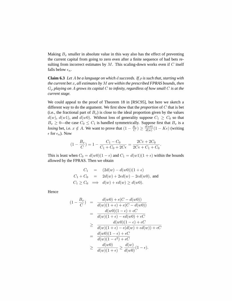
Claim 6.3 LetA be a language on whichd succeeds. Ifρ is such that, starting withthe current betx, all estimates byM are within the prescribed FPRAS bounds, thenGρ playing onA grows its capitalC to infinity, regardless of how smallC is at thecurrent stage.

We could appeal to the proof of Theorem 18 in [RSC95], but here we sketch adifferent way to do the argument. We first show that theproportionof C that is bet(i.e., the fractional part ofBx) is close to the ideal proportion given by the valuesd(w), d(w1), andd(w0). Without loss of generality supposeC1 ≥ C0 so thatBx ≥ 0—the caseC0 ≤ C1 is handled symmetrically. Suppose first thatBx is alosingbet, i.e.x /∈ A. We want to prove that(1− Bx

C ) ≥ d(w0)d(w) (1−Kε) (writing

ε for εn). Now

(1− BxC

) = 1− C1 − C0

C1 + C0 + 2Cε=

2Cε+ 2C0

2Cε+ C1 + C0.

This is least whenC0 = d(w0)(1− ε) andC1 = d(w1)(1 + ε) within the boundsallowed by the FPRAS. Then we obtain

C1 = (2d(w)− d(w0))(1 + ε)C1 + C0 = 2d(w) + 2εd(w)− 2εd(w0), and

C1 ≥ C0 =⇒ d(w) + εd(w) ≥ d(w0).

Hence

(1− BxC

) =d(w0) + ε(C − d(w0))

d(w)(1 + ε) + ε(C − d(w0))

=d(w0)(1− ε) + εC

d(w)(1 + ε)− εd(w0) + εC

≥ d(w0)(1− ε) + εC

d(w)(1 + ε)− ε(d(w) + εd(w)) + εC

=d(w0)(1− ε) + εC

d(w)(1− ε2) + εC

≥ d(w0)d(w)(1 + ε)

≥ d(w)d(w0)

(1− ε).

The last line follows from the identityb, x ≥ 0 ∧ b ≥ a =⇒ a+xb+x ≥

ab , and

d(w0)(1−ε) = a ≥ b = d(w)(1−ε2 becaused(w)(1+ε) ≥ d(w0). That finishesthis case, withK = 1.

The case of a winning bet is not quite symmetrical. We want to show(1 +BxC ) ≥ d(w1)

d(w) (1−Kε). We have

(1 +BxC

) = 1 +C1 − C0

C1 + C0 + 2Cε=

2Cε+ 2C1

2Cε+ C1 + C0.

This is least whenC1 = d(w1)(1− ε) andC0 = d(w0)(1 + ε) within the boundsallowed by the FPRAS. Then we obtain

C0 = (2d(w)− d(w1))(1 + ε)C1 + C0 = 2d(w) + 2εd(w)− 2εd(w1), and

C1 ≥ C0 =⇒ d(w1) ≥ d(w)(1 + ε).

The last line is the part that isn’t symmetrical. Now we get:

(1 +BxC

) =d(w1) + ε(C − d(w1))

d(w)(1 + ε) + ε(C − d(w1))

Now we want to use the identity

(x < 0 ∧ (b+ x) > 0 ∧ a ≥ b) =⇒ a+ x

b+ x≥ a

b.

If C < d(w1), this is satisfied withx = ε(C − d(w1)), a = d(w1), andb =d(w)(1 + ε). This is becauseC1 ≥ C0 =⇒ a ≥ b, andb + x > d(w) + εd(w) −εd(w1) ≥ d(w)(1− ε) sinceC > 0 andd(w1) ≤ 2d(w). Thus we get

(1 +BxC

) ≥ d(w1)d(w)(1 + ε)

≥ d(w1)d(w)

(1− ε)

and we’re home, again withK = 1. Now what ifC ≥ d(w1)? In this analysis,that impliesC ≥ d(w)(1 + ε). We can wave this case away by reasoning that if thecurrent capital is already doing that much better than the “true value”d(w) thenthere is nothing to prove. Or we can makeG always keep some of its capital inreserve, so thatC stays less thand(w) unless the FPRAS estimates are violated onthe high side. Finally, we could also change the “+2εC” in the denominator of (3)to something else, at the cost of makingK higher.

(Remark. One interesting thing about this argument is that the inequalitiesresulting from the worst-case choices ofC1 andC0, namelyd(w1) ≥ d(w)(1 + ε)

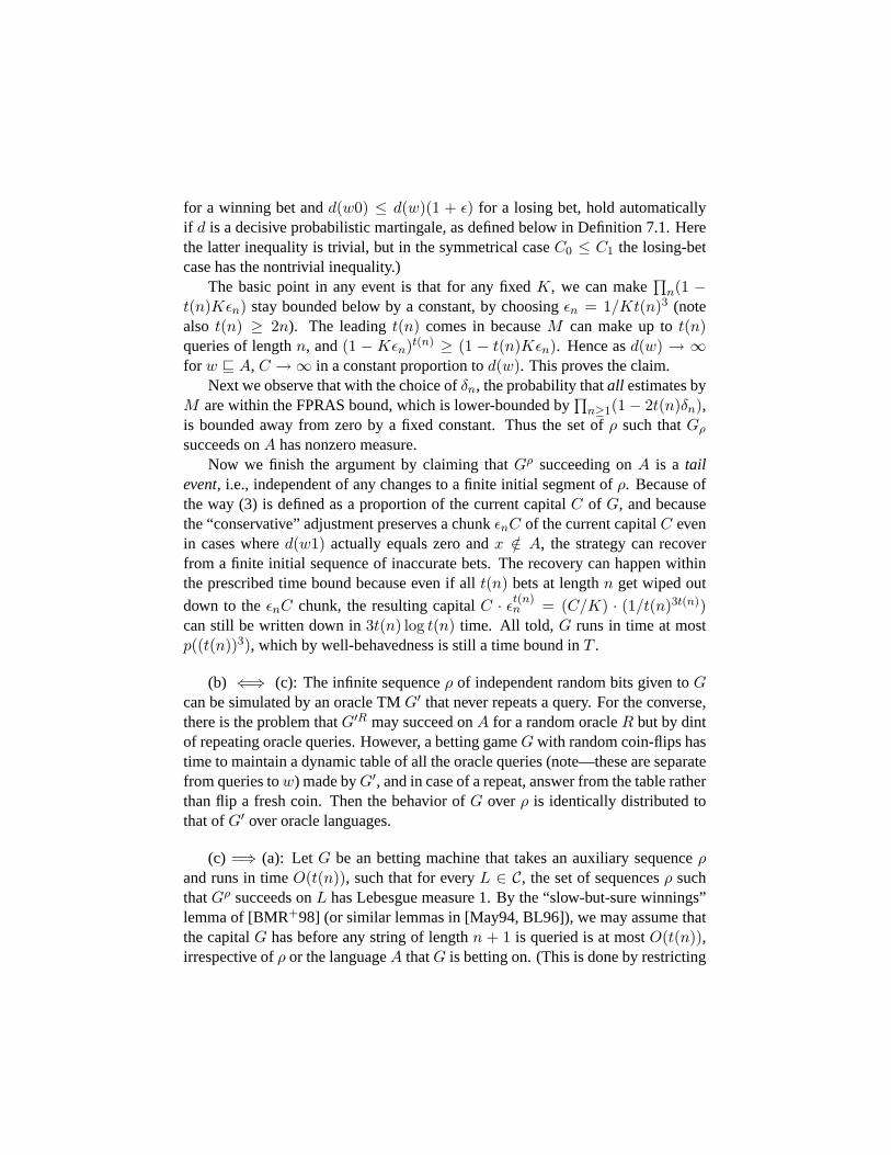
for a winning bet andd(w0) ≤ d(w)(1 + ε) for a losing bet, hold automaticallyif d is a decisive probabilistic martingale, as defined below in Definition 7.1. Herethe latter inequality is trivial, but in the symmetrical caseC0 ≤ C1 the losing-betcase has the nontrivial inequality.)

The basic point in any event is that for any fixedK, we can make∏n(1 −

t(n)Kεn) stay bounded below by a constant, by choosingεn = 1/Kt(n)3 (notealso t(n) ≥ 2n). The leadingt(n) comes in becauseM can make up tot(n)queries of lengthn, and(1 −Kεn)t(n) ≥ (1 − t(n)Kεn). Hence asd(w) → ∞for w v A, C →∞ in a constant proportion tod(w). This proves the claim.

Next we observe that with the choice ofδn, the probability thatall estimates byM are within the FPRAS bound, which is lower-bounded by

∏n≥1(1− 2t(n)δn),

is bounded away from zero by a fixed constant. Thus the set ofρ such thatGρsucceeds onA has nonzero measure.

Now we finish the argument by claiming thatGρ succeeding onA is a tailevent, i.e., independent of any changes to a finite initial segment ofρ. Because ofthe way (3) is defined as a proportion of the current capitalC of G, and becausethe “conservative” adjustment preserves a chunkεnC of the current capitalC evenin cases whered(w1) actually equals zero andx /∈ A, the strategy can recoverfrom a finite initial sequence of inaccurate bets. The recovery can happen withinthe prescribed time bound because even if allt(n) bets at lengthn get wiped out

down to theεnC chunk, the resulting capitalC · εt(n)n = (C/K) · (1/t(n)3t(n))

can still be written down in3t(n) log t(n) time. All told, G runs in time at mostp((t(n))3), which by well-behavedness is still a time bound inT .

(b) ⇐⇒ (c): The infinite sequenceρ of independent random bits given toGcan be simulated by an oracle TMG′ that never repeats a query. For the converse,there is the problem thatG′R may succeed onA for a random oracleR but by dintof repeating oracle queries. However, a betting gameG with random coin-flips hastime to maintain a dynamic table of all the oracle queries (note—these are separatefrom queries tow) made byG′, and in case of a repeat, answer from the table ratherthan flip a fresh coin. Then the behavior ofG overρ is identically distributed tothat ofG′ over oracle languages.

(c) =⇒ (a): LetG be an betting machine that takes an auxiliary sequenceρand runs in timeO(t(n)), such that for everyL ∈ C, the set of sequencesρ suchthatGρ succeeds onL has Lebesgue measure 1. By the “slow-but-sure winnings”lemma of [BMR+98] (or similar lemmas in [May94, BL96]), we may assume thatthe capitalG has before any string of lengthn + 1 is queried is at mostO(t(n)),irrespective ofρ or the languageA thatG is betting on. (This is done by restricting

G to never bet more than one unit of its capital.)For everyn, the computation ofGρ alongA can use at mostt(n) bits of ρ

before all queried strings of lengthn are queried. Thus a finite initial segmentσ v ρ of lengtht(n) suffices to determine the capital thatGρ has at any point priorto querying a string of lengthn + 1. Now define, for anyw of lengthN ≈ 2n,d(w) to be the average, over all sequencesσ of lengtht(n), of the capital thatGσ

has after it has queried all strings (that it queries) whose membership is specifiedbyw. It is immediate thatd is a martingale.

Claim 6.4 C ⊆ S∞[d].

Proof. (of Claim 6.4). Suppose there is a languageL ∈ C on whichd does notsucceed. Then there is a natural numberm such that for allw v L, d(w) ≤ m.Now for eachN define

ON := ρ : (∃w v L, |w| ≤ N)Gρ(w) ≥ 2m , (4)

and finally defineO = ∪wvLOw. Then eachON is topologically open in thespace 0, 1 ω, becauseρ ∈ ON is witnessed by a finite initial segmentσ v ρof lengtht(n), which is long enough to fix the computationGσ(w). Also clearlyO1 ⊆ O2 ⊆ O3 . . ., so thatO is an increasing union of theON .

Finally and crucially, eachON has measure at most1/2. This is because themeasure ofON is just the proportion ofσ of lengtht(n) such thatGσ(w) ≥ 2m.If this proportion were> 1/2, then the overall averaged(w) would be> m,contradicting the choice ofL andm.

Thus we have an increasing countable union of open sets, each of measure atmost1/2. It follows that their unionO has measure at most1/2. The easiest wayto see this is to writeO = O1 ∪ (O2 \ O1) ∪ (O3 \ O2) ∪ . . . . This makesO adisjoint union of piecesON \ ON−1, and boundsµ(O) by an infinite sum whosesummands are non-negative and whose partial sums are all≤ 1/2. Hence the sumconverges to a value≤ 1/2.

Hence the complementA ofO has measure at least1/2. For everyρ ∈ A, andeveryN , ρ /∈ ON . This implies that for allw v L (of any lengthN ), Gρ(w) ≤2m. It follows thatGρ does not succeed onL. Thus the set ρ : L /∈ S∞[Gρ] has measure at least1/2, contradicting the hypothesis that ρ : L ∈ S∞[Gρ] hasmeasure one.

Finally, we note thatd has a full time-T randomized approximation scheme.This is simply because the averages can be estimated to within a desiredpoly(t(n))mean error by makingpoly(t(n)) random samples, in time bounded by a polyno-mial in t(n). More details follow.

Let A be a language along whichG succeeds, fix a prefixw of A of length2n, and for an auxiliary sequenceσ of length t(n), let Gσ,w denote the capitalthatGσ has prior to querying any string of lengthn + 1. As mentioned above,we will assume that the “slow-but-sure” construction of [BMR+98] has been ap-plied toG. This ensures that the capitalG has before querying any string of lengthn + 1 is at mostO(t(n)) (irrespective of its auxiliary sequence and the languagethat it is betting on). Givenε andδ, we will divide theO(t(n))-sized range into

O(t(n)) tiny intervals of constant size. PickO( (t(n))2

ε log t(n)δ ) random auxiliary

sequencesσ, and for each sequenceσ, computeGσ,w and find out which interval

this capital falls within. This computation takes timet(n)O( (t(n))2

ε log t(n)δ ) =

(t(n))O(1)O(1ε log 1

δ ). By standard Chernoff bounds, for any intervalI, with prob-ability 1− δ/Ω(t(n)), the probability thatGσ,w falls within I is accurate to withinε/Ω((t(n))2). Thus with probability at least1−O(t(n))(δ/Ω(t(n))), the probabil-ities are accurate to withinε/Ω((t(n))2) for every interval. Therefore, the estimateof d(w) made this way is accurate withinO(t(n))×O(t(n))× ε/Ω((t(n))2) = εwith probability at least1− δ.

In the above proof of (c)=⇒ (a), by replacing “2m” by “Km” for largerK in (4),we can show that the measure ofO arbitrarily close to zero. Hence we have: givenG andL, if ρ : Gρ coversL does not have measure 1, then it has measure 0.This seems curious, because “Gρ coversL” is not in general a “tail event.” Nev-ertheless, nothing in this part of the argument requires this to be a tail event—noreven thatG be a betting game! Thus our proof actually shows more generally that“FPRAS” is a robust notion of computing real-valued functions onΣ∗, namely thatit is equivalent to the “measure one” type definitions that are possible.

7 Measuring Sub-Exponential BP Time Classes Directly

Now we can carry over the definitions and results of Section 4 to sub-exponentialtime boundst(n), starting right away with the notion of decisiveness.

Definition 7.1. A martingaled is t(n)-decisiveif there existsk > 0 such that forall w, takingN = |w| andn = dlog2eN , eitherd(w1) − d(w) = 0 or |d(w1) −d(w)| ≥ 1/t(n)k.

Recall that a familyT of time bounds is well-behaved if for allt ∈ T andk > 0,the functiont(n)k also belongs toT . The threshold1/t(n)k is fine enough to maketime-t(n) martingales that bet below it fail to succeed, and coarse enough to enable

a time-T (n) randomized approximation scheme’s estimates to be finer than it, withhigh probability.

Although giving proof details here is somewhat redundant with Section 4, wewant to make it fully clear that the results really do carry over to sub-exponentialtime bounds.

Proposition 7.1 Decisive probabilistic martingales for well-behaved time boundsT satisfy measure axiomsM2 andM3. That is:

(a) For any languageA ∈ BPTIME[T (n)], there is a decisiveBPTIME[T (n)]martingaled such thatA ∈ S∞[d].

(b) For every decisiveBPTIME[T (n)] martingaled, there is a languageA ∈BPTIME[T (n)] such thatA /∈ S∞[d].

Proof. (a) Taket ∈ T such thatA ∈ BPTIME[t(n)]. We can find a probabilisticTM MA running in timeO(t(n)) such that for allx of any lengthn, Pr[MA(x) =A(x)] > 1 − 1/22t(n), which is bounded below by1 − 1/22n sincet(n) ≥ n.Now let d be the martingale induced by the lex-limited betting game that playsonly on strings0n and bets all of its capital onA(0n). Thend is trivially decisive,and is approximable usingMA in timeO(t(n)), so it is a time-T (n) probabilisticmartingale that coversA.

(b) DefineA to be the diagonal language of the martingaled, viz. A = x :d loses money onx . We need to show thatA ∈ BPTIME[T (n)]. TakeM be atime-T (n) randomized approximation scheme that with high probability approxi-mates (the betting strategy used by)d to within 1/2t(n)k, and letMA acceptx iffM says that the bet onx is negative. Owing to decisiveness, wheneverx ∈ A,M will say “negative” with high probability, and similarly forx /∈ A. HenceA ∈ BPTIME[T (n)].

Proposition 7.2 Probabilistic time-T martingales satisfyM1–finite unions andM2, and satisfyM1–infinite unions for classes closed under finite variations.

Proof. The proof forM2 is immediate by the last proof. The proof for the finitecase ofM1 is the same as that of (a) in Proposition 4.1. For infinite unions, wecombine the construction in Proposition 5.4 with the idea for finite unions. Byrunning approximations for valuesd1(w), . . . , dn(w) so that each comes within afactor of(1± εn/n) with probability at least(1− δn/n), we can approximate thedesired weighted sum ofd1(w), . . . , dn(w) to within a factor of(1 ± εn), with

probability at least(1− δn). Settingεn = 1/t(n)3 andδn similarly does the trick.

Theorem 7.3 For all individual time boundst ∈ T (n), BPTIME[t(n)] can becovered by a time-T (n) probabilistic martingale.

Proof. TakeP1, P2, . . . to be a standard recursive enumeration of probabilistic Tur-ing machines that run in timet(n). Now play the randomized lex-limited bettinggameM defined as follows.M divides its initial capitalC0 = 1 into infinitelymany “shares”sk = 1/2k2 for k ≥ 1 (with an unused portion1 − π2/12 of C0

left over). Each sharesk is assigned toPk, maintains its own capital, and plays oninfinitely many stringsx of the formx = 0n, wheren is divisible by2k but not by2k+1. Then no two shares play on the same string.

To play sharesk on a stringx = 0n, M uses its random bits to simulatePkt(n)-many times, treating acceptance as+1 and rejection as−1, and letsν be thesample mean of the results.M then bets a portionν/2 of the current capital ofsharesk with the same sign asν. ThenM runs in timeO(t(n)2).

As in the proof of Theorem 4.2, For anyPk that has bounded error probability,a measure-one set of random sequences makeν > 1/2 for all but finitely many0n ∈ L(Pk) andν < −1/2 for all but finitely many0n ∈∼ L(Pk). Hence for anysuch sequence, sharesk survives a possible finite sequence of losses and eventuallygrows to+∞. HenceM succeeds onL(Pk).

The corollary now follows directly from the measure, rather than relying onpadding results.

Corollary 7.4 If probabilistic time-T (n) martingales can be simulated by decisiveones, then for allt(n) ∈ T , BPTIME[t(n)] 6= BPTIME[T (n)].

If the decisive simulation is uniform enough to apply to any well-behavedT ,then

BPTIME[O(n)] ⊂ BPP ⊂ BPTIME[qpoly ], and

BPE ⊂ BPEXP,

all of which are unknown and possibly contradicted by oracle evidence.Cai et al. [CLL+95] define the notion of afeasible generatorto be a prob.

polynomial time machine that, on input1n, generates a string of lengthn accord-ing to some probability distributionD = Dn∞n=0. In that paper we raised the

following question of whether every feasible generator has amonic refinement: forevery feasible generatorM , is there a machineM ′ such that for alln, there existsy ∈ 0, 1n s.t. Pr[M ′(1n) = y] > 3/4? We also studied the analogue of thisquestion for arbitrary generators (i.e., non-feasible generators), and showed that,in general, this is impossible.

Further, in [CLL+95] we observed a connection between this problem and thenotion of fully polynomial time randomized approximation scheme (FPRAS), andestablished the following two facts:

(1) For every functionf with an FPRAS, there is a machineMf such that foreveryx andε there are two valuesy1 andy2 such that(1 − ε)f(x) ≤ y1 ≤ y2 ≤(1 + ε)f(x) and such that for anyδ, Pr[Mf (x, ε, δ) ∈ y1, y2] > 3/4.

(2) If there is a machineMf that achieves an effect similar to (1) with just onevaluey instead of two valuesy1 andy2, then every feasible generator has a monicrefinement.

It follows from our results that if every FPRAS has a symmetry breaking algo-rithm as in (2), then one would obtain a tight BPTIME hierarchy.

8 Conclusions

We have defined a natural and interesting candidate notion of probabilistic mea-sure. The notion has already been applied to “natural proofs” and a simulation of“betting games,” from which it follows that it measures classes not known to bemeasured deterministically. We have proved it to be fairly robust and appropriatefor BPTIME classes. We have tied questions about its suitability to the longstand-ing open problem of whether there is a tightBPTIME hierarchy. One footnote onthe latter deserves measure. It follows from our work that one of the following istrue:

• #P 6= P

• BPP has a nontrivial time hierarchy, viz. for somek, and all c,BPTIME[nc] 6= BPTIME[nkc].

While this can be argued directly by lettingk be something like the time for com-puting the permanent assuming#P = P, the connection through measure is inter-esting.

References

[Amb86] K. Ambos-Spies. Relativizations, randomness, and polynomial re-ducibilities. InProceedings, First Annual Conference on Structure inComplexity Theory, volume 223 ofLect. Notes in Comp. Sci., pages23–34. Springer Verlag, 1986.

[AS94] E. Allender and M. Strauss. Measure on small complexity classes,with applications for BPP. InProc. 35th Annual IEEE Symposium onFoundations of Computer Science, pages 807–818, 1994.

[AS95] E. Allender and M. Strauss. Measure on P: Robustness of the notion.In Proc. 20th International Symposium on Mathematical Foundationsof Computer Science, volume 969 ofLect. Notes in Comp. Sci., pages129–138. Springer Verlag, 1995.

[BFT95] H. Buhrman, L. Fortnow, and L. Torenvliet. Using autoreducibilityto separate complexity classes. In36th Annual Symposium on Foun-dations of Computer Science, pages 520–527, Milwaukee, Wisconsin,23–25 October 1995. IEEE.

[BG81a] C. Bennett and J. Gill. Relative to a random oracleA, PA 6= NPA 6=coNPA with probability 1.SIAM J. Comput., 10:96–113, 1981.

[BG81b] C. Bennett and J. Gill. Relative to a random oracleA, PA 6= NPA 6=coNPA with probability 1.SIAM J. Comput., 10:96–113, 1981.

[BL96] H. Buhrman and L. Longpre. Compressibility and resource boundedmeasure. In13th Annual Symposium on Theoretical Aspects of Com-puter Science, volume 1046 oflncs, pages 13–24, Grenoble, France,22–24 February 1996. Springer.

[BMR+98] H. Buhrman, D. van Melkebeek, K. Regan, D. Sivakumar, andM. Strauss. A generalization of resource-bounded measure, with anapplication. InProc. 15th Annual Symposium on Theoretical Aspectsof Computer Science, volume 1373 ofLect. Notes in Comp. Sci.,,pages 161–171. Springer Verlag, 1998.

[CLL+95] J.-Y. Cai, R. Lipton, L. Longpre, M. Ogihara, K. Regan, andD. Sivakumar. Communication complexity of key agreement on lim-ited ranges. InProc. 12th Annual Symposium on Theoretical Aspects

of Computer Science, volume 900 ofLect. Notes in Comp. Sci., pages38–49. Springer Verlag, 1995.

[CSS97] J.-Y. Cai, D. Sivakumar, and M. Strauss. Constant depth circuits andthe Lutz hypothesis. InProc. 38th Annual IEEE Symposium on Foun-dations of Computer Science, pages 595–604, 1997.

[FS89] L. Fortnow and M. Sipser. Probabilistic computation and linear time.In Proc. 21st Annual ACM Symposium on the Theory of Computing,pages 148–156, 1989.

[FS97] L. Fortnow and M. Sipser. Retraction of “Probabilistic computationand linear time”. InProc. 29th Annual ACM Symposium on the Theoryof Computing, page 750, 1997.

[GZ97] O. Goldreich and D. Zuckerman. Another proof that BPP⊆ PH (andmore). Technical Report TR97–045, Electronic Colloquium on Com-putational Complexity (ECCC), September 1997.

[HILL91] J. Hastad, R. Impagliazzo, L. Levin, and M. Luby. Construction of apseudo-random generator from any one-way function. Technical Re-port 91–68, International Computer Science Institute, Berkeley, 1991.

[JS89] M. Jerrum and A. Sinclair. Approximating the permanent.SIAM J.Comput., 18:1149–1178, 1989.

[JVV86] M. Jerrum, L. Valiant, and V. Vazirani. Random generation of com-binatorial structures from a uniform distribution.Theor. Comp. Sci.,43:169–188, 1986.

[KL83] R. Karp and M. Luby. Monte-Carlo algorithms for enumeration andreliability problems. InProc. 24th Annual IEEE Symposium on Foun-dations of Computer Science, pages 56–64, 1983.

[Ko83] K. Ko. On the definitions of some complexity classes of real numbers.Math. Sys. Thy., 16:95–109, 1983.

[KV87] M. Karpinski and R. Verbeek. Randomness, provability, and the sepa-ration of Monte Carlo time and space. InComputation Theory andLogic, volume 270 ofLect. Notes in Comp. Sci., pages 189–207.Springer Verlag, 1987.

[Lut92] J. Lutz. Almost everywhere high nonuniform complexity.J. Comp.Sys. Sci., 44:220–258, 1992.

[May94] E. Mayordomo.Contributions to the Study of Resource-Bounded Mea-sure. PhD thesis, Universidad Polytecnica de Catalunya, Barcelona,April 1994.

[NW88] N. Nisan and A. Wigderson. Hardness vs. randomness. InProc. 29thAnnual IEEE Symposium on Foundations of Computer Science, pages2–11, 1988.

[RR97] A. Razborov and S. Rudich. Natural proofs.J. Comp. Sys. Sci., 55:24–35, 1997.

[RSC95] K. Regan, D. Sivakumar, and J.-Y. Cai. Pseudorandom generators,measure theory, and natural proofs. InProc. 36th Annual IEEE Sym-posium on Foundations of Computer Science, pages 26–35, 1995.

[RV97] R. Rettinger and R. Verbeek. BPP equals BPLINTIME under an oracle(extended abstract), November 1997.

[Str97] M. Strauss. Measure on P—strength of the notion.Inform. and Comp.,136:1–23, 1997.