probabilistic inference modulo theories - sri …braz/presentations/hr 2015.pdfprobabilistic...
TRANSCRIPT

Rodrigo de Salvo Braz Artificial Intelligence Center - SRI International
joint work with Ciaran O’Reilly
Artificial Intelligence Center - SRI International
Vibhav Gogate University of Texas at Dallas
Rina Dechter
University of California, Irvine
Probabilistic Inference Modulo Theories
Hybrid Reasoning Workshop – IJCAI 2015 - July 26, 2015
Probabilistic Programming for Advanced Machine Learning
Outline
• Two extremes: logic and probabilistic inference
• Probabilistic inference in Graphical Models
– Factorized joint probability distribution
– Marginalization
– Variable elimination
– Mainstream probabilistic inference representation
• Logic Inference
– Theories
– Inference: satisfiability
– DPLL
– DPLL(T)
• Symbolic Generalized DPLL Modulo Theories (SGDPLL(T))
• Experiments
• Conclusion

Two extremes: logic and probabilistic inference • Logic – Initial mainstream approach to AI: represent knowledge declaratively,
have a system using it
– Can use rich theories: data structures, numeric constraints, functions
– Basic logic does not offer treatment for uncertain knowledge
• Probabilistic Inference – Follows the idea of representing knowledge declaratively and having a
system use it
– Very good treatment of uncertainty
– Poor representation, equivalent to discrete variables with equality, lacking interpreted functions (data structures, arithmetic) and even uninterpreted non-nullary functions (friends(X,Y))
– Way to use such constructs is to ground them into tables or formulas
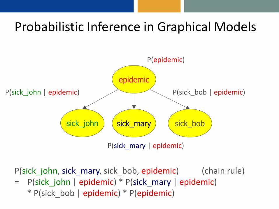
Probabilistic Inference in Graphical Models
epidemic
P(sick_john, sick_mary, sick_bob, epidemic) (chain rule) = P(sick_john | epidemic) * P(sick_mary | epidemic) * P(sick_bob | epidemic) * P(epidemic)
sick_john sick_mary sick_bob
P(sick_bob | epidemic)
P(epidemic)
P(sick_john | epidemic)
P(sick_mary | epidemic)
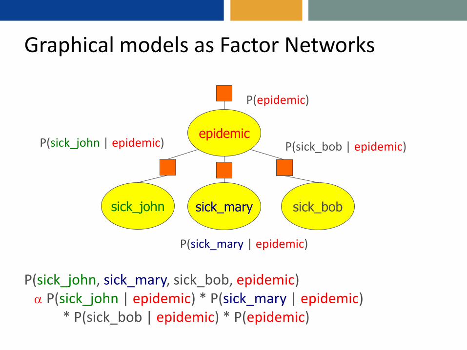
Graphical models as Factor Networks
epidemic
P(sick_john, sick_mary, sick_bob, epidemic) P(sick_john | epidemic) * P(sick_mary | epidemic) * P(sick_bob | epidemic) * P(epidemic)
sick_john sick_mary sick_bob
P(sick_bob | epidemic)
P(epidemic)
P(sick_john | epidemic)
P(sick_mary | epidemic)
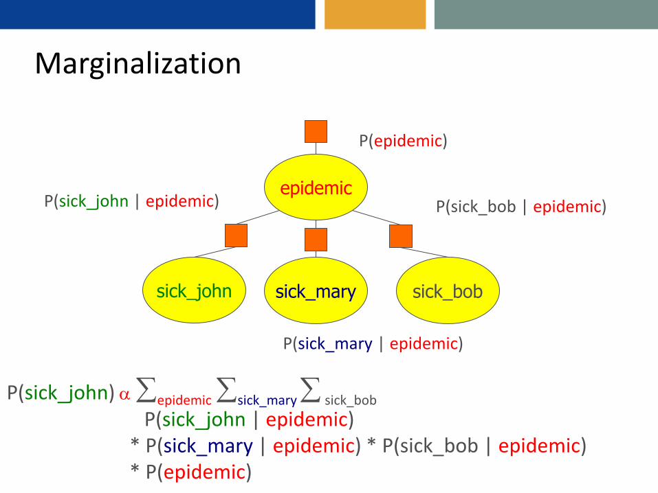
Marginalization
epidemic
P(sick_john) epidemic sick_mary sick_bob P(sick_john | epidemic) * P(sick_mary | epidemic) * P(sick_bob | epidemic) * P(epidemic)
sick_john sick_mary sick_bob
P(sick_bob | epidemic)
P(epidemic)
P(sick_john | epidemic)
P(sick_mary | epidemic)

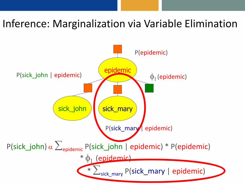
Inference: Marginalization via Variable Elimination
epidemic
sick_john sick_mary sick_bob
P(sick_bob | epidemic)
P(epidemic)
P(sick_john | epidemic)
P(sick_mary | epidemic)
P(sick_john) epidemic P(sick_john | epidemic) * P(epidemic)
* sick_mary P(sick_mary | epidemic)
* sick_bob P(sick_bob | epidemic)

Inference: Marginalization via Variable Elimination
epidemic
sick_john sick_mary
1(epidemic)
P(epidemic)
P(sick_john | epidemic)
P(sick_mary | epidemic)
P(sick_john) epidemic P(sick_john | epidemic) * P(epidemic)
* sick_mary P(sick_mary | epidemic)
* 1 (epidemic)
Inference: Marginalization via Variable Elimination
epidemic
sick_john sick_mary
1(epidemic)
P(epidemic)
P(sick_john | epidemic)
P(sick_mary | epidemic)
P(sick_john) epidemic P(sick_john | epidemic) * P(epidemic)
* 1 (epidemic)
* sick_mary P(sick_mary | epidemic)
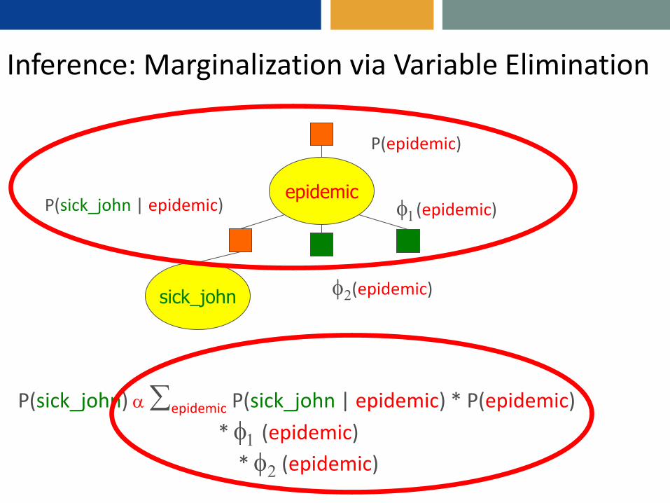
Inference: Marginalization via Variable Elimination
epidemic
sick_john
1(epidemic)
P(epidemic)
P(sick_john | epidemic)
P(sick_john) epidemic P(sick_john | epidemic) * P(epidemic)
* 1 (epidemic)
* 2 (epidemic)
2(epidemic)
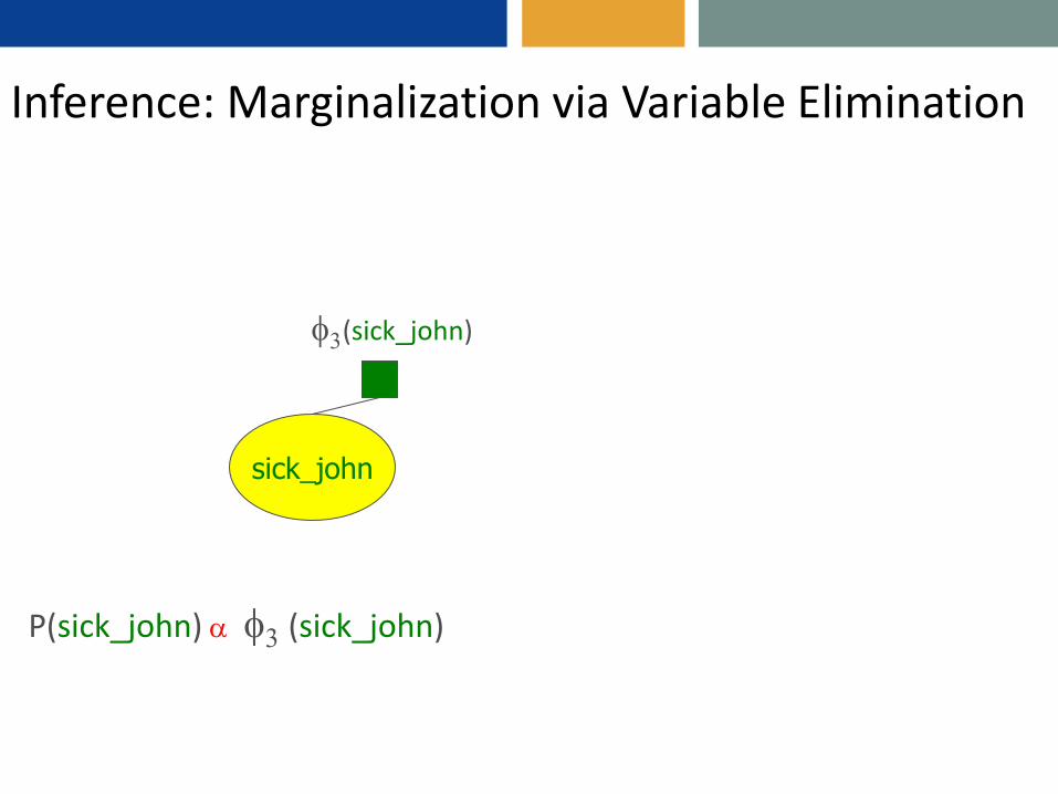
Inference: Marginalization via Variable Elimination
sick_john
3(sick_john)
P(sick_john) 3 (sick_john)
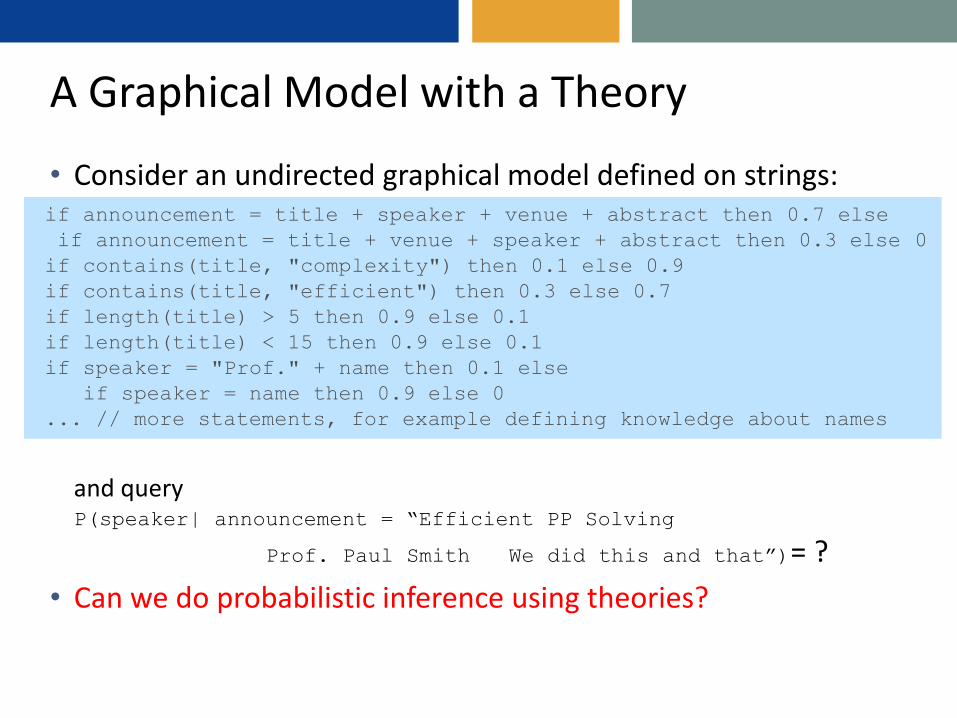
A Graphical Model with a Theory
• Consider an undirected graphical model defined on strings:
and query P(speaker| announcement = “Efficient PP Solving
Prof. Paul Smith We did this and that”)= ?
• Can we do probabilistic inference using theories?
if announcement = title + speaker + venue + abstract then 0.7 else
if announcement = title + venue + speaker + abstract then 0.3 else 0
if contains(title, "complexity") then 0.1 else 0.9
if contains(title, "efficient") then 0.3 else 0.7
if length(title) > 5 then 0.9 else 0.1
if length(title) < 15 then 0.9 else 0.1
if speaker = "Prof." + name then 0.1 else
if speaker = name then 0.9 else 0
... // more statements, for example defining knowledge about names
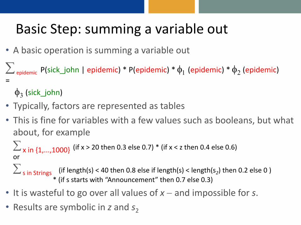
Basic Step: summing a variable out
• A basic operation is summing a variable out
epidemic P(sick_john | epidemic) * P(epidemic) * 1 (epidemic) * 2 (epidemic)
=
3 (sick_john)
• Typically, factors are represented as tables
• This is fine for variables with a few values such as booleans, but what about, for example
x in {1,...,1000} (if x > 20 then 0.3 else 0.7) * (if x < z then 0.4 else 0.6)
or
s in Strings (if length(s) < 40 then 0.8 else if length(s) < length(s2) then 0.2 else 0 )
* (if s starts with “Announcement” then 0.7 else 0.3)
• It is wasteful to go over all values of x and impossible for s.
• Results are symbolic in z and s2
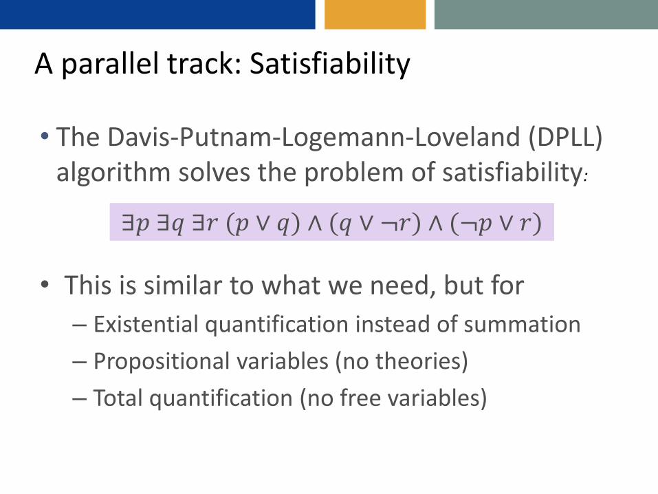
A parallel track: Satisfiability
• The Davis-Putnam-Logemann-Loveland (DPLL) algorithm solves the problem of satisfiability:
∃𝑝 ∃𝑞 ∃𝑟 (𝑝 ∨ 𝑞) ∧ (𝑞 ∨ ¬𝑟) ∧ (¬𝑝 ∨ 𝑟)
• This is similar to what we need, but for
– Existential quantification instead of summation
– Propositional variables (no theories)
– Total quantification (no free variables)
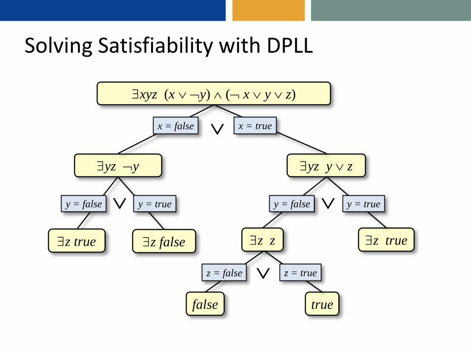
Solving Satisfiability with DPLL
xyz (x y) ( x y z)
yz y yz y z
z true z false z z z true
x = false x = true
y = false y = true y = false y = true
false true
z = false z = true
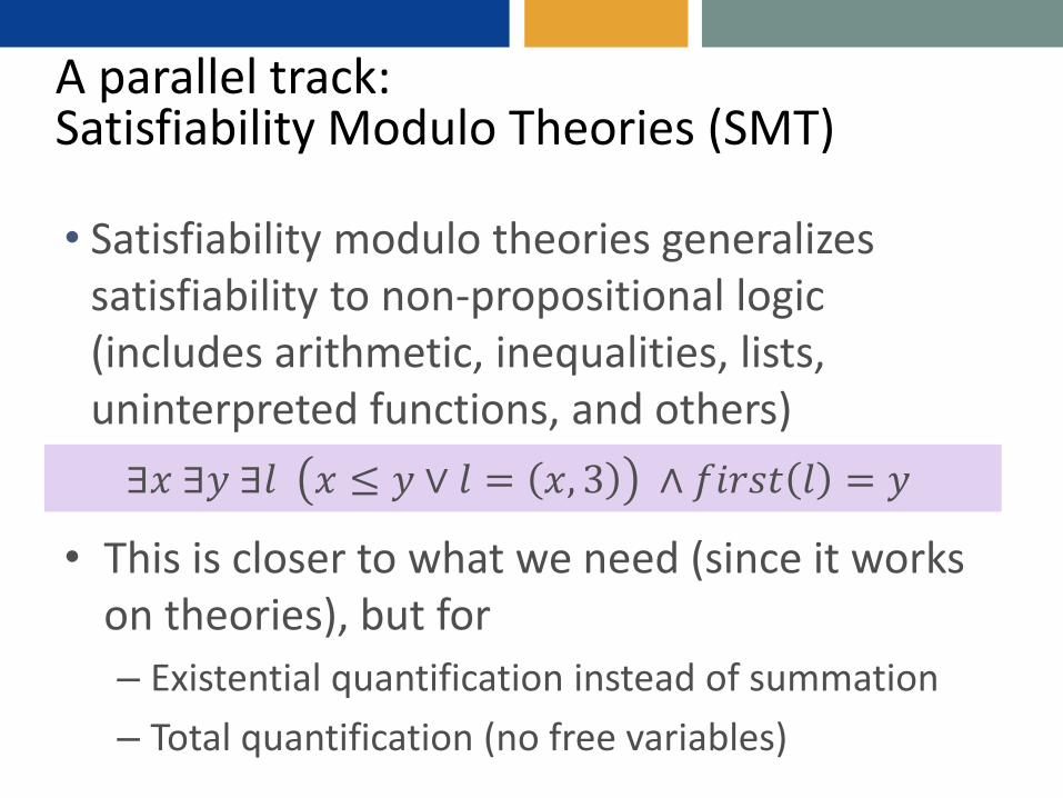
A parallel track: Satisfiability Modulo Theories (SMT)
• Satisfiability modulo theories generalizes satisfiability to non-propositional logic (includes arithmetic, inequalities, lists, uninterpreted functions, and others)
∃𝑥 ∃𝑦 ∃𝑙 𝑥 ≤ 𝑦 ∨ 𝑙 = 𝑥, 3 ∧ 𝑓𝑖𝑟𝑠𝑡 𝑙 = 𝑦
• This is closer to what we need (since it works on theories), but for
– Existential quantification instead of summation
– Total quantification (no free variables)
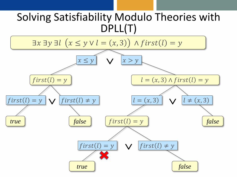
Solving Satisfiability Modulo Theories with DPLL(T)
∃𝑥 ∃𝑦 ∃𝑙 𝑥 ≤ 𝑦 ∨ 𝑙 = 𝑥, 3 ∧ 𝑓𝑖𝑟𝑠𝑡 𝑙 = 𝑦
𝑓𝑖𝑟𝑠𝑡 𝑙 = 𝑦 𝑙 = 𝑥, 3 ∧ 𝑓𝑖𝑟𝑠𝑡 𝑙 = 𝑦
true false
𝑥 ≤ 𝑦 𝑥 > 𝑦
𝑓𝑖𝑟𝑠𝑡 𝑙 = 𝑦 𝑓𝑖𝑟𝑠𝑡 𝑙 ≠ 𝑦 𝑙 = 𝑥, 3 𝑙 ≠ 𝑥, 3
𝑓𝑖𝑟𝑠𝑡 𝑙 = 𝑦 false
𝑓𝑖𝑟𝑠𝑡 𝑙 = 𝑦 𝑓𝑖𝑟𝑠𝑡 𝑙 ≠ 𝑦
false true

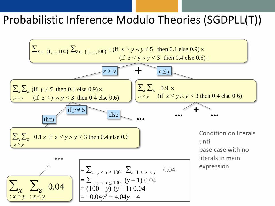
Our solution: Probabilistic Inference Modulo Theories
• Similar to SMT, but based on – Summation (or other quantifiers) instead of
– Partial quantification (free variables)
x{1,…,100}z{1,…,100} (if x > y y ≠ 5 then 0.1 else 0.9)
(if z < y y < 3 then 0.4 else 0.6)
• Note that y is a free variable
• Summed expression is not Boolean
• Language is not propositional (≠, <, …)
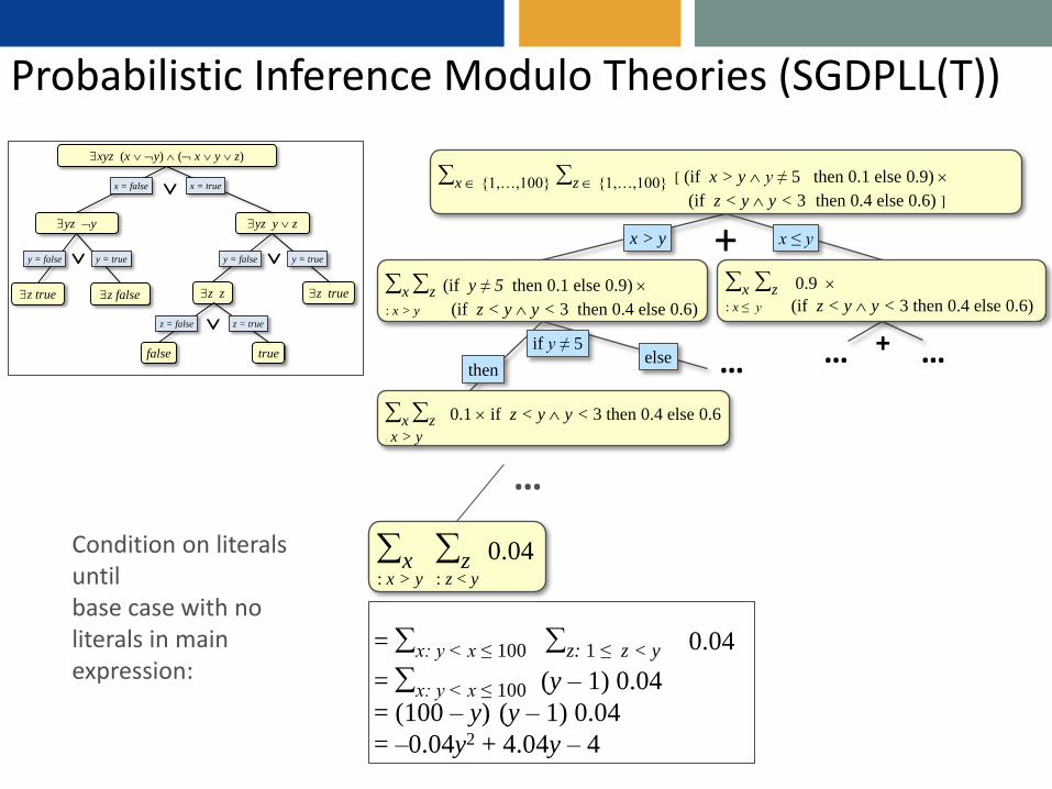
Probabilistic Inference Modulo Theories (SGDPLL(T))
xyz (x y) ( x y z)
yz y yz y z
z true z false z z z true
x = false x = true
y = false y = true y = false y = true
false true
z = false z = true
…
x {1,…,100} z {1,…,100} [ (if x > y y ≠ 5 then 0.1 else 0.9)
(if z < y y < 3 then 0.4 else 0.6) ]
x z (if y ≠ 5 then 0.1 else 0.9)
: x > y (if z < y y < 3 then 0.4 else 0.6)
x ≤ y +
x z 0.1 if z < y y < 3 then 0.4 else 0.6
: x > y
+ … …
x z 0.9
: x ≤ y (if z < y y < 3 then 0.4 else 0.6)
x > y
else then
if y ≠ 5
x z 0.04 : x > y : z < y
= x: y < x ≤ 100 z: 1 ≤ z < y 0.04
= x: y < x ≤ 100 (y – 1) 0.04
= (100 – y) (y – 1) 0.04
= –0.04y2 + 4.04y – 4
…
Condition on literals until base case with no literals in main expression:
Probabilistic Inference Modulo Theories (SGDPLL(T))
= x: y < x ≤ 100 z: 1 ≤ z < y 0.04
= x: y < x ≤ 100 (y – 1) 0.04
= (100 – y) (y – 1) 0.04
= –0.04y2 + 4.04y – 4
Condition on literals until base case with no literals in main expression
…
x {1,…,100} z {1,…,100} [ (if x > y y ≠ 5 then 0.1 else 0.9)
(if z < y y < 3 then 0.4 else 0.6) ]
x z (if y ≠ 5 then 0.1 else 0.9)
: x > y (if z < y y < 3 then 0.4 else 0.6)
x ≤ y +
x z 0.1 if z < y y < 3 then 0.4 else 0.6
: x > y
+ … …
x z 0.9
: x ≤ y (if z < y y < 3 then 0.4 else 0.6)
x > y
else then
if y ≠ 5
x z 0.04 : x > y : z < y
…
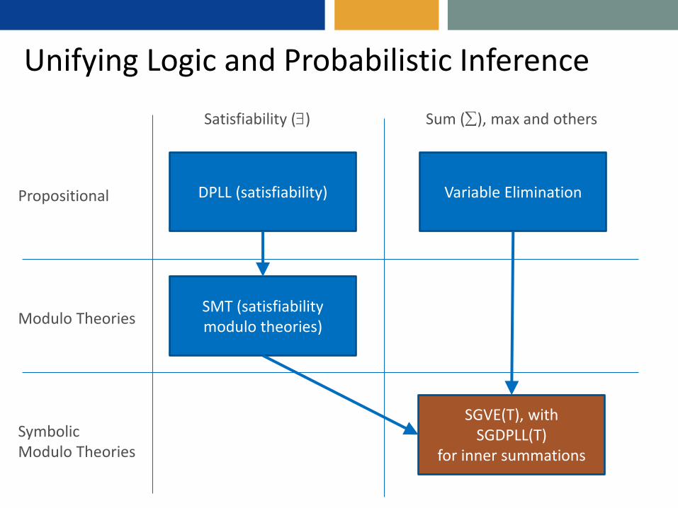
Unifying Logic and Probabilistic Inference
Variable Elimination DPLL (satisfiability)
SMT (satisfiability modulo theories)
SGVE(T), with SGDPLL(T)
for inner summations
Propositional
Modulo Theories
Symbolic Modulo Theories
Satisfiability () Sum (), max and others
Evaluation
• Generated random graphical models defined on equalities on bounded integers
• Evaluated against VEC (Gogate & Dechter 2011), a state-of-the-art graphical model solver, after grounding into tables with increasing random variable domain sizes
• For domain of size 16, our solver was already 20 times faster than VEC.
Final Remarks on SGDPLL(T)
• It is symbolic (S)
• It is generic (not only Boolean expressions) (G)
• Can use theories (T)
• Can re-use SMT techniques – Satisfiability solvers
– Modern SAT solver techniques: – Unit propagation and Watched literals
– Clause learning
• Requires new solvers on theories for base cases (at least as powerful as model counting)

Thanks!