1

Probabilistic assessments in relationship

with Safety Integrity Levels by using Fault Trees

Y. Dutuit, F. Innal,

IMS/LAPS, Université Bordeaux 1, 33405 Talence Cedex, FRANCE

A. Rauzy

IML/CNRS, 163, avenue de Luminy, 13288 Marseille Cedex 09, FRANCE

J.-P. Signoret

Total, CSTJF, Avenue Larribau, 64018 Pau Cedex, FRANCE

Abstract: In this article, we study the assessment of Safety Integrity Levels of Safety

Instrumented System by means of Fault Trees. We focus on functions with a low demand rate.

For these functions, the appropriate measure of performance is the so-called probability of

failure on demande (PFD) or probability of not functioning on demand. In order to calculate

accurately the average PFD as per IEC 61508 standard, we introduce distributions for

periodically tested components into Fault Tree models. We point out the specific problems

raised by the assessment of Safety Integrity Levels, which restrict the use of the formulae

proposed in the standard. Among these problems there is the fact that SIL should be assessed

by considering the time-dependent behavior of the system unavailability in addition to its

average value. We check, on a simple pressure protection system, the results obtained by means

of the fault tree approach against those obtained by means of stochastic Petri nets with

predicates.

Notations & Acronyms:

BDD: Binary Decision Diagrams

HIPPS: High Integrity Pressure Protection System

MCS: Minimal Cutsets

PFD: Probability of not Functioning on Demand

PN: Petri Nets

SIL: Safety Integrity Level

2

SIS: Safety Instrumented System

1. Introduction

The concept of safety integrity levels (SIL) was introduced during the development of IEC

61508 [1]. This standard deals with instrumented systems that have a safety function (SIS) to

perform. The concept of SIL is thus a measure of the confidence with which the system can be

expected to perform their safety function.

The standard points out that safety functions can be required to operate in quite different ways.

Many such functions are only called upon at a low frequency / have a low demand rate. On the

other hand, there are functions which are of a frequent or continuous use. This leads to the

definition of two kinds of SIL.

For functions with a low demand rate, the accident rate is the combination of two parameters:

first, the frequency of demands coming from the equipment under control, second the

probability of not functioning on demand (PFD) of the SIS. The appropriate measure of

performance of the function is the latter (i.e. the mean unavailability of the SIS).

For functions with a high demand rate or functions that operate continuously, the accident rate

is the so-called probability of failure per hour, which is not clearly defined in the standard.

This measure of performance is anyway out of the scope of this article.

Note that we prefer the term "Probability of not Functioning on Demand" to the one used in the

standard, namely "Probability of Failure on Demand", because the latter can be confused with

(or to be restricted to) the probability of failure due to the demand itself which is usually noted

γ (gamma). The former has the advantage to involve both the failure due to the demand itself

and the failure in functioning occurred before the demand [2]. The Safety Integrity Level L of a

system S at time t is derived straight from the unavailability QS(t) by means of the following

formula.

L

SL tQ −+− <≤ 10)(10 )1(

The standard IEC 61508 considers actually levels 1 to 4. In presence of periodically tested

components, QS shows a saw tooth curve behavior. We advocate here that, if the mean value is

necessary to characterize QS, it is far from sufficient. We propose a model of failure probability

distribution for periodically tested components. We show by means of examples how the

3

unavailability of the system may vary with the various parameters of the model (non negligible

duration of tests, availability of components available during tests, failure rates during and

between tests, repair rates, probability of bad restarts after tests, and so on). We propose an

algorithm to assess the unavailability throughout a mission time (the problem is to select a

suitable number of dates at which this quantity is to be assessed). We also show how staggering

the test impacts the maximum PFD and how it decreases the common cause failures impact.

Complex systems like SIS can be assessed accurately by means of formalisms like Petri nets or

Markov graphs. However, the design of models in such formalisms is difficult and error prone.

Fault Trees are much easier to handle for the practitioner, but provide only approximated

results. Therefore, if the Fault Tree approach provides results that are accurate enough, it

should be preferred. It remains that, in a research phase, the former kind of models should be

used to check the accuracy of the latter. This is the reason why we give here both.

The remainder of this article is organized as follows. Section 2 proposes a parametric

distribution for the probability of failure of periodically tested components. Section 3 presents

a simple illustrative example. Section 4 sketches a Petri net model for this example. Section 5

discusses the specific problems raised by the assessment of Safety Integrity Levels when using

fault trees models. Finally, section 6 presents some experimental results obtained with a Fault

Tree model against those obtained with the Petri net model.

2. Periodically Tested Components

The main aim of this article is to show the ability of the Fault Tree approach to model the

failure logic of any SIS and to compute its average PFD. If it is well-known that the

computation of the top-event probability is easily performed by using Fault Tree when all basic

events have “classical” distributions (such as the negative exponential distribution), some

problem can occur when these basic events correspond to periodically inspected and tested

components. Unfortunately, safety instrumented systems involve generally many such

components. Therefore, a general model of periodically tested component (see [3], [4]) must be

elaborated and implemented to make it possible to perform realistic computations of PFD and

SIL. We show hereafter how to deal with this problem and present a generic and parametric

distribution for such components.

4

2.1. Phases

A periodically tested component goes through an alternation of phases. It is successively in

operation, test and maintenance (when a test reveals a failure). There are actually three types of

phases. The first one corresponds to the first operation period that spreads from time 0 to the

date of the first test. The second type corresponds to test periods. Finally, the last type

corresponds to operation periods (between tests). The first phase is distinguished from those of

the third type because in many real-life systems with several components, the dates of first tests

of the components may be shifted, even if the components are otherwise identical and tested

with the same period.

In the sequel, we call θ the date of the first test, τ the time between the beginning of two

consecutive tests and π the duration of the test period. Figure 1 illustrates the meaning of the

parameters θ, τ and π. Each test is performed at dates θ+n.τ, where n is any non negative

integer operation periods spread from dates θ+n.τ+π to θ+(n+1).τ.

Note that it is more convenient in practice to define the time between two consecutive tests than

the duration of the operation period (which is, according to our notation, τ−π). Note also that,

tests are considered to be instantaneous (π=0) by numerous authors. This is in fact relevant only

when the component remains available for its safety function or if the installation under

protection is shut down during the tests. The repair time is also considered very often as to be

negligible. Again, this is a safe approximation only if the installation under protection is shut

down during repair. Therefore in most of the cases θ and repair rate have to be modeled

properly. It is worth to note that, in practice, the test duration is often the top contributor to the

unavailability of a periodically tested component.

2.2. Multi phase Markov Graphs approach

In order to design a probability distribution for periodically tested components, we made the

following assumptions.

• Periods of test and operation alternate as described in the previous section.

• Failures are detected (and therefore repair started) only after an inspection (test) period.

• Components show a Markovian behavior, i.e. they have a constant failure rate – λ

during operation periods, λ* during test periods – and a constant repair rate µ. After a

repair, components are assumed to be as good as new.

5

• Components may be available or not during test period. We use the Boolean indicator x

to tell whether the component is available (x = 1) or not (x = 0).

• There is a (possibly null) probability that the test fails the component (probability of

failure due to the test). As before, we call γ this probability. It is a pure probability of

failure on demand (i.e. due to a demand)

• The coverage of the test may be imperfect, i.e. the failure (if any) of the component is

detected with a probability σ.

• Finally, there is a probability w that the component is badly restarted after a test.

Table 1 summarizes the different parameters of the probability distribution. Other assumptions

could have been done but those we have chosen encompass most of the problem encountered

and are far beyond what is commonly taken under consideration.

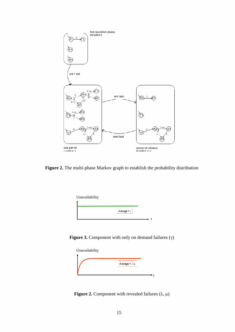
The multi-phase Markov graph for the probability distribution is given in Figure 2. Ai’s, Fi’s,

Ri’s states correspond respectively to states where the component is available, failed and in

repair. The index “i” does not refer to a considered phase. As explained below, it enables us to

distinguish between states which can be successively occupied within a given phase.

Continuous arrows correspond to Markovian transitions and dashed arrows to immediate

transitions. States with only immediate outgoing transitions are transient states (i.e. without

actual duration).

In the first phase, the distribution is a simple exponential law of parameter λ. The component is

assumed to work at t = 0. We added states F1 and R1 for the sake of uniformity. However, the

probability to be in these states is null at the beginning of this phase, but the component can fail

during this first phase (transition λ between states A1 and F2).

At the end of a given phase the component may be either in working, failed or repair states. In

order to simplify the presentation of the Markov graphs, similar states have been split. For

example, at the end of an operation phase, the working state is split between A1 and A3 (A2 is

a transient state) and failed state between F1, F2 and F3. The states A1 (respectively F1) and

A3 (respectively F2 and F3) are temporarily distinguished because they are reached by

different ways. There are also three repair states R1, R2 and R3. The probabilities of these

states are used to calculate the initial probabilities of the following test phase. The probability

to be in A1 (respectively F1) at the beginning of a test phase is then the sum of the probabilities

to be in A1 or A3 (respectively F1, F2 and F3) at the end of an operation phase. The probability

to be in R1 at the beginning of the test phase is simply the probability to be in repair at the end

6

of the previous phase. Similarly, the probability to be in R1 at the beginning of a given

operation phase is the sum of the probabilities to be in states R1, R2 and R3 at the end of the

previous test period. This probability is indeed very low. In this case, the test is cancelled. The

same principle is applied when the phase changes from a phase test to an operation phase.

If the component enters available into an operation phase, the distribution follows an

exponential law of parameter λ. If the component enters failed into this phase, it remains failed

up to the next test phase.

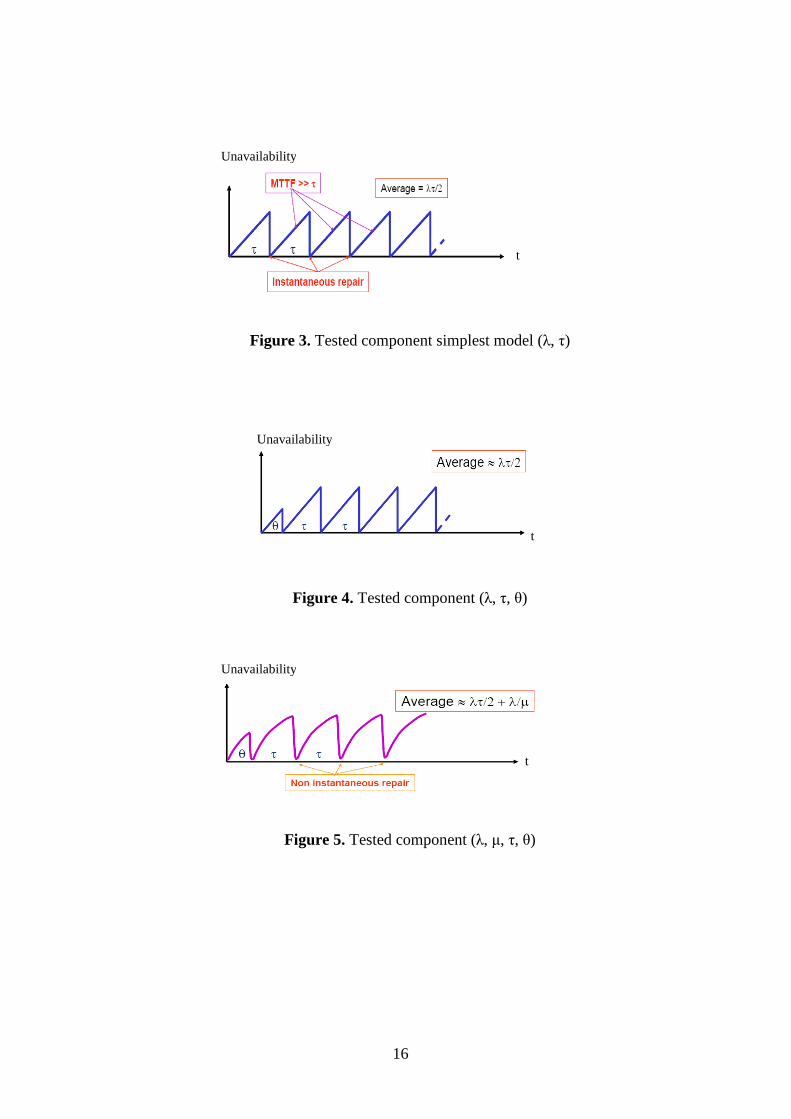
To illustrate the effect of the above parameters on the behavior of a single component, we give

in Figure 3 to Figure 9 the curves of its instantaneous unavailability Q(t) and its average value

according to the parameters taken into account [5]. These distributions make it possible to

calculate the probability of failure of periodically tested components. Combined through the

fault tree this makes it possible to calculate the probability of occurrence of the top event (i.e.

the system unavailability). By performing this calculation for a sufficient number of dates over

a given period of time, we establish a curve of the instantaneous unavailability of the system

under study. Its average value over the considered period is obtained by integration. The saw

tooth curves are typical of systems with periodically tested components. It should be noticed

that the instantaneous unavailability of the system is quite chaotic and goes through minimum

and maximum that are far from the mean value. We shall also observe in section 6 that it

spreads over several SIL zones.

3. Example: A simple Pressure Protection System

Pressure Protection Systems are a typical example of safety instrumented systems. Such a

system is pictured in Figure 10. This SIS is a simple but typical HIPPS (High Integrity Pressure

Protection System) devoted to protect downstream part of a production system against an

overpressure due to its upstream part.

Three pressure sensors detect when the pressure increases over a specified threshold. These

three sensors send the information to a logic solver (LS) implementing a 2oo3 voting logic.

Then, the logic solver sends a signal to solenoid valves SVs. When receiving the signal, the

solenoid valves release the hydraulic pressure maintaining the shutdown valves SDVs open.

Strong springs close these valves. When the shutdown valves are closed, the pressure drops in

the downstream part of the system.

7

As usual, this HIPPS is made up of three subsystems in series.

The first one is the set of three pressure sensors-transmitters. Their undetected dangerous

failures are revealed only by means of proof tests performed every month (730 hours). Their

common failure rate is 4.4e-7 h-1. During its proof test, sensors are unavailable.

The second subsystem consists of the 2oo3 logic solver LS. Its detected failure rate and its

repair rate are respectively 5e-6 h-1 and 0.125 h-1.

The third subsystem has a redundant architecture 1oo2. Each channel is made up of a solenoid

valve SVi and a shutdown valve SDVi. The dangerous undetected failure rate of the former

type is 8.8e-7 h-1. Each SVi is tested for the first time after one month of operation and, after

that, every two months (1460 hours). They are unavailable during the test duration (1 hour).

SDVs exhibit two failure modes. The movement failures are detected by partial stroking tests.

The valve movement failure rate is 2.66e-6 h-1. The first test is performed after respectively one

month for SDV1 and two months for SDV2. After that, each SDVi is tested every two months.

The production is stopped after failures detection. SDV closure failures are detected only by

full stroking tests. The failure rate of this second failure mode is 8.9e-7 h-1. The first full

stroking test occurs after three months (respectively six months) for SDV1 (respectively SDV2)

and the test intervals between the following tests are the same for both SDV1 and SDV2,

namely six months. As previously, the production is stopped after failures detection. Therefore,

the risk disappears during repair. These repairs are, in fact, hidden.

All the reliability data and characteristics are respectively summarized in Tables 2 and 3.

4. A Stochastic Petri Nets model with predicates

The fault tree method is widely used because of its simplicity and its efficiency. However, in

the case of SIS, it can be only an approximation, for this kind of systems involves often

components with mutually exclusive failure modes. In order to validate the Fault Tree approach

we advocate in this article, we developed a stochastic Petri net model for the SIS presented in

the previous section.

This model is actually a combination of Petri nets depicted in Figure 11 to Figure 18 and

variables gathered in Table 4. This kind of Petri nets, so-called stochastic Petri nets with

predicates, look like the conventional ones, but have an extended expression and computation

power. For example, new attributes are affected to the transitions such as elaborated guards

(pre-condition messages) enabling them, affectations (post-condition messages) which update

8

the variables used in the model, and so on. Another advantage of these Petri nets is their ability

to perform modular models. Because they are out of the scope of this paper, the basic features

of Petri nets modeling are not described here, but they can be found in many articles already

published (see, for instance, references [6], [7]).

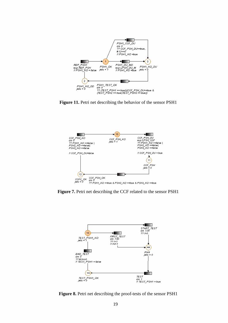
However, the Petri net model we give deserves some explanations. Petri nets for sensors PSHi

(i=1,2,3) and shutdown valves SDVi (i=1,2) are divided respectively into three and four subsets.

Initially all the guards are false, all components work and since no test has been performed, i.e.,

places 1, 12, 13, 26, 46 … are marked. A possible evolution of the HIPPS components can be

described as follows.

A CCF which impacts the three sensors first occurs, i.e., the transition between places 10 and

11 is fired when its delay “exp LPSH_CCF” is elapsed. This firing is enabled because at least

one of the guards of the considered transition (?? PSHi_KO == false) is true. The token

disappears from place 10 and a token appears in place 11. The assignment (!! CCF_PSH_DU =

true) is performed. This induces immediately the firing of the transition between places 1 and 3.

The token leaves place 1 and a token marks place 3. The assignment (!! PSH1_KO = true) is

performed. Now, the sensor PSH1 is failed. Sensors PSH2 and PSH3 are failed as well, due

to CCF. The variable PSHs_PFD is set to 1, because no token remains in places 1, 4 and 7.

This common failure causes the whole system failure of the HIPPS (the value of the variable

HIPPS_PFD equals 1). It is inhibited, i.e., it is unable to act if a demand occurs from the

equipment under control. This failure state remains until the first proof-test related to the

sensors occurs (until now, no test has been performed: the variable I is null). This first test is

started after 730 hours of operation. The transition between places 13 and 44 is then fired. The

token leaves place 13 and a token appears in place 44. After 1 hour, the test duration is elapsed

and the transition between places 44 and 14 is fired. Thus, place 44 has no token and place 14

is marked. The transition between places 3 and 2 is now fired. A token marks place 2. That

means the repair of PSH1 is started. Simultaneously the transition between places 14 and 13 is

triggered; this indicates that the first proof test related to PSH1 is achieved. When the repair of

PSH1 ends, the transition between places 2 and 1 is fired and token appears again in place 1.

The evolution will continue as previously described.

We have performed 106 Monte Carlo trials to simulate the behavior of the HIPPS over a

mission time of 20000 hours to obtain an average PFD equal to 1.636e-3 ± 5.4e-6, which is

very close to the result previously obtained by means of Fault Tree model (1.639e-3, see

below).

9

The good agreement between the above results is not as obvious as it appears, as explained

hereafter. A first cause which could generate a significant difference between FT and PN

numerical results lies in the fact that FT computes an exact top-event probability (if BDD

coding is used) from the probabilities allocated to its basic events, when PN approach only

gives an estimation (with a confidence interval if necessary). A second cause concerns the used

probabilities of basic eevnts. To satisfy the drastic condition which contraints the quantitative

exploitation of any FT, all its basic events are considered as independent events. But it is not

the case, because some of concerned components have not a binary behavior and then not

independent failure modes (DD and DU). Moreover, for each type of components (SV, SDV

and PSH) individual and common cause failures are also mutually exclusive events. Contrary to

FT, PN models, coupled with Monte Carlo simulation, are able to take into account the true

charachteristics of any type of components. In spite of the above differences between FT and

PN models, their mumerical results related to the studied system are close. This is due in

particular to the pre-eminence of the CCF contributions and, in general, to the low value of the

used failure rates.

5. Assessment by means of Fault Trees

As the reader can see, Petri net models, even for simple systems, are quite complex to design

and to maintain. That is the reason why fault tree models are preferable. The assessment of

Safety Integrity Level by means of fault trees raises however a number of specific problems.

A common mistake consists in calculating the top event probability from average values of

components’ unavailability (with the latter’s approximated as λτ/2). The more the system is

redundant the system, the more the result is non conservative. Such a twist in calculation is

indeed unacceptable when dealing with safety systems.

The curves pictured in Figure 5 to Figure 9 illustrate another important issue. The

unavailability curves of periodically tested components and of the whole system show a cyclic

behavior. These curves go through minima and maxima that differ by orders of magnitude.

Therefore, their mean may be a very rough indicator (even if completed with first orders

moments). Similarly, the SIL of the system, if assessed only based on mean unavailability’s,

may be questionable. This phenomenon is even accentuated if the system embeds periodically

tested components for which the test period cannot be considered as instantaneous and that are

not available during the test (in this case the maximum values may go to 1). The experiments

we performed on various systems convinced us that it is necessary to look at whole curves of

10

unavailability to get relevant information. If the notion of SIL as per IEC 61508 is indeed still

of interest, it seems to be insufficient to obtain a good picture of the actual undertaken risk.

Therefore, we suggest assessing the percentage of time the system spends in each SIL zone for

obtaining a more accurate indication. Such information is more concise than a full curve and is

an appropriate measure of the performance of the safety function.

Due to its saw tooth shape, the unavailability of the system must be calculated for a sufficient

number of instants spreading over the mission time in order to get a good picture of its curve

and produce a good calculation of its average value. Most of the fault tree assessment tools

calculate the unavailability of the top event through the minimal cut sets (MCS) approach.

When the system under study is large, the fault tree is large as well and admits many (often too

many) MCS. Therefore, cutoffs are applied to focus on the most important MCS. These cutoffs

discard MCS with too low probabilities. However, in the case of a system with periodically

tested components, the probabilities of MCS evolve periodically through the time. So, the set

of relevant MCS at time t1 may be completely different from the set of relevant MCS at time t2.

To overcome this problem the solution could be to (re)compute MCS at each considered instant.

However, this would be definitely too time consuming. Fortunately this problem is solved by

the Binary Decision Diagram (BDD) approach (see e.g. [8]). With this approach, the BDD is

computed once for all. Then, the system unavailability is assessed in linear time with respect to

the size of the BDD.

In order to get a curve precise enough to accurately calculate its average, we need to assess the

system unavailability at many different times and including all singularities. This is indeed

costly, even with the BDD approach. In order to save computation time, we developed a

heuristic to create an accurate sample. This heuristics consists in looking for all singularity time

points (i.e. the beginnings and ends of test periods) and to add more time points by means of a

dichotomized search between these singularities (an intermediate point is added when the

values at the two points under study differ by a predefined amount).

6. Numerical Results

The Fault Tree model related to the HIPPS is depicted in Figure 19. This Fault Tree is very

small, but presents clearly the different kinds of failures related to components, i.e. the intrinsic

or independent failures and the common cause failures (CCF). The two failure modes of the

shutdown valves (SDVs fail to move and fail to close) also appear.

11

Figure 20 shows the curve of the instantaneous unavailability of the HIPPS over a limited

period of time, but sufficient to highlight its periodical aspect. It must be noted that this curve

has been truncated in magnitude, because its maxima go to 1.

The mean value of the unavailability, computed over 20000 hours, which measures the PFD of

the HIPPS, is 1.639e-3. Therefore, the system, as per IEC 61508 is considered as SIL 2. At first

glance, this may seem surprising because the curve of Figure 20 shows that the system spends

most of the time in SIL 3 zone and, more precisely, in the range of magnitude [1e-4, 5e-4]. This

is confirmed by reading Table 5 which gives the percentage of time spent by the system in each

SIL zone.

In fact, there is no contradiction between the above results (average PFD value versus time

spent in SIL 3 zone). This apparent incoherency disappears if one keeps in mind the maximum

value periodically reached by the system unavailability. These peaks are due to the

unavailability of some components during their proof tests. Their impact on system PFD is

deciding, even if the test duration is very short (1 hour). This important point must be

emphasized because it is not taken into account in the analytical formulae proposed in IEC

61508-6 standard. Another tricky case must be considered which illustrates one of the problems

we highlighted in a previous section and in reference [9]. Let us imagine a system which

spends most of the time in SIL 2 zone and more than 10% of the mission time in SIL 1, which

is far from negligible and can be dangerous. Moreover, if this system also spends more than 3%

of its mission time in SIL3 zone, less risk at one moment does not compensate more risk at

another one. With periodically tested system, when the threshold of a wrong SIL zone is

trespassed the system remains in this wrong zone until the next test and this can be for a long

delay when components are tested every 5 years, for example.

In the previous section, we mention that the choice of an accurate sample (of computation

dates) is an important issue. To illustrate this point, we assess the mean of the unavailability of

the system with samples of different sizes. Namely, we computed QS at 0, dt, 2dt, 3dt… and so

on until 20000 with 6 different values of the step dt, with and without adding the singularity

points (in our case the test dates ± ε). Table 6 gives the mean value of QS we obtained. Note

that the results are indicated with 4 significant digits only for comparison purpose. These

results illustrate the importance of the choice of a good sample. Without adding singularity

points, results may be definitely inaccurate if the sample is not large enough (which means, in

this very simple case, several hundred of points). By adding the singularity points, we can get

accurate results even with relatively small samples (made on few dozens of points).

12

Note that in the petroleum fields, SIL3 is at least required for High Integrity Pressure Protection

Systems and only very short excursions in SIL2 zone with low magnitude are allowed.

Therefore, the simple system analyzed here as example would not be acceptable as HIPPS.

7. Conclusion

In this article, we present the methodology that we have developed to assess the so-called

PFDavg in relationship with Safety Integrity Levels of Safety Instrumented System by means

of Fault Trees. We focused on functions with a low demand rate, for which the appropriate

measure of performance is the unavailability or probability of not functioning o demand (i.e.

the so-called Probability of Failure on Demand as per IEC 61508). We pointed out some

important issues raised by the assessment of systems that embed periodically tested

components. We suggested ways to get rid of these problems.

A very simple example has been analyzed under some common hypotheses adopted by

reliability engineers. This experiment shows that, even in this extremely simplified case, the

saw tooth nature of the instantaneous unavailability cannot be handled properly by using

averaged values.

The solutions we proposed in this article relies on the BDD technology. We implemented new

algorithms dedicated to the assessment of SIL in the Aralia Workshop software package, our

Fault Tree assessment tool. For the sake of verification, we compared results provided by

Aralia with those obtained by means of Monte Carlo simulations based on a Petri Net models.

These comparisons showed that results obtained by means of Fault Trees are almost identical to

those obtained by the more elaborated methods.

Our future works will be performed in two directions:

• Explore the case of systems with high demand rate. This involves the assessment of the

"failure rate" as required by the IEC61508 standard but the relevant parameter is, in fact,

the system unconditional failure intensity. Several mathematical and technical problems

are expected.

• Analyze the impact on spurious failures of the various standard requirements and

specially those in relationship with architectural constraints and the so-called safe

failure fraction (SFF).

13

8. References

[1] IEC 61508. Functional safety of electric/ electronic/ programmable electronic safety-

related systems. Parts 1–7; October 1998 – May 2000.

[2] Innal F., Dutuit Y., Rauzy A., Signoret J.P. An attempt to better understand and to better

apply somme of the recommendations of IEC 61508 standard. 30th ESReDA Seminar on

Reliability of Safety-Critical Systems. SINTEF/NTNU, Trondheim, Norway, June 7-8,

2006.

[3] Signoret J.P. Etude probabiliste des systèmes périodiquement testés : Rapport

DGEP/SES/ARF/JPS/co n° 86. 009 ELF Aquitaine Production (in French), Nov.1986.

[4] Dutuit Y., Rauzy A., Signoret J.P., Thomas P. Disponibilité d’un système en attente et

périodiquement testé. Procedings of the QUALITA 99 Conference (in French), pp.367-

375, Paris, France, March 25-26, 1999.

[5] Signoret J.P. High Integrity Protection System (HIPS) – Overcoming SIL calculation

difficulties. TOTAL document, Pau, 2004.

[6] Malhotra M., Trivedi K.S., Dependability Modeling using Petri Nets, IEEE Trans.

Reliability, vol.44, n° 3, 1995, pp. 428-440.

[7] Dutuit Y., Châtelet E., Signoret J.P., Thomas P., Dependability modelling and evaluation

by using stochastic Petri nets: application to two test cases, Reliability Engineering and

System Safety, vol.55, n° 2, 1997, pp. 117-124.

[8] Rauzy A. New Algorithms for Fault Trees Analysis. Reliability Engineering & System

Safety, 05(59):203–211, 1993

[9] Dutuit Y., Rauzy A., Signoret J.P. Probabilistic assessments in relationship with Safety

Integrity Levels by using Fault Trees. Procedings of the ESREL 2006 Conference, vol.2,

pp.1619-1624, Estoril, Portugal, September 18-22, 2006.

14

Figure 1. The three phases of a periodically tested component

λ Failure rate when the component is working.

λ* Failure rate when the component is tested.

µ Repair rate (once a test showed that the component is failed).

τ Delay between two consecutive tests.

θ Delay before the first test.

γ Probability of failure due to the (beginning of the) test.

π Duration of the test.

x Indicator of the component availability during the test (1 available, 0 unavailable).

σ Test coverage: probability that the test detects the failure, if any.

ω Probability that the component is badly restarted after a test or a repair.

Table 1. Parameters of the probability distribution of periodically tested components.

15

Figure 2. The multi-phase Markov graph to establish the probability distribution

Unavailability

t

Figure 3. Component with only on demand failures (γ)

Unavailability

t

Figure 2. Component with revealed failures (λ, µ)

16

Unavailability

t

Figure 3. Tested component simplest model (λ, τ)

Unavailability

t

Figure 4. Tested component (λ, τ, θ)

Unavailability

t

Figure 5. Tested component (λ, µ, τ, θ)

17

Unavailability

t

Figure 6. Tested component (λ, µ, γ, τ, θ)

Unavailability

t

Figure 9. Tested component (λ, µ, γ, τ, θ, π) unavailable during tests

Figure 10. A simple HIPPS architecture

18

Parameters

Components

Failure Mode λDD (h-1) λDU (h-1) DC Test interval

(h)

Time to First Test

(h)

β

(CCF) %

(applied to

failure

rate)

PSH1 Fails to send a

signal 0 4.4e-7 0 730 730

PSH2 Fails to send a

signal 0 4.4e-7 0 730 730

PSH3 Fails to send a

signal 0 4.4e-7 0 730 730

5

SDV1 Failure to move 0 2.66e-6 0 1460 730

SDV2 Failure to move 0 2.66e-6 0 1460 1460 10

SDV1 Failure to fully

close 0 8.9e-7 0 4380 2190

SDV2 Failure to fully

close 0 8.9e-7 0 4380 4380

10

SV1 Failure to move 0 8.8e-7 0 1460 730

SV2 Failure to move 0 8.8e-7 0 1460 1460 10

Logic solver Failure to act 5.0e-6

Table 2. Reliability parameters of components

Parameters

Components

Repair time

(hours)

Test

Duration

(hours)

Item

available

during test

PSHs 8 1 no

SDVs 8 0 yes

SVs 1 1 no

Logic

Solver 8

Table 3. Other component reliability characteristics

19

Figure 11. Petri net describing the behavior of the sensor PSH1

Figure 7. Petri net describing the CCF related to the sensor PSH1

Figure 8. Petri net describing the proof-tests of the sensor PSH1

20

Figure 9. The Petri net describing the behavior of the logic solver LS

Figure 10. Petri net describing the behavior of the shutdown valve SDV1

21

Figure 11. Petri net describing the proof-tests (FM) of the shutdown valve SDV1

Figure 12. Petri net describing the CCF related to the shutdown valve SDV1

22

Figure 18. Petri net describing the proof-tests (FC) of the shutdown valve SDV1

Type Name Definition/ Initial value Real BETA_PSH 0.05 Real BETA_SDV 0.1 Real BETA_SV 0.1 Integer I, J, K, L, M, N, O, P, Q 0 Real LAMBDA_PSH_DU 4.40E-07 Real LAMBDA_SDV_FC_DU 8.90E-07 Real LAMBDA_SDV_FM_DU 2.66E-06 Real LAMBDA_SV_DU 8.80E-07 Real LLS_DD 5.00E-06 Real LPSH_CCF (LAMBDA_PSH_DU)*BETA_PSH Real LPSH_DU_IN (LAMBDA_PSH_DU)*(1.0-BETA_PSH) Real LSDV_CCF_FC LAMBDA_SDV_FC_DU*BETA_SDV Real LSDV_CCF_FM LAMBDA_SDV_FM_DU*BETA_SDV Real LSDV_FC_DU_IN LAMBDA_SDV_FC_DU*(1.-BETA_SDV) Real LSDV_FM_DU_IN LAMBDA_SDV_FM_DU*(1.-BETA_SDV) Real LSV_CCF LAMBDA_SV_DU*BETA_SV Real LSV_DU_IN LAMBDA_SV_DU*(1.-BETA_SV) Real REP_LS 0.125 Real REP_PSH 0.125 Real REP_SDV 0.125 Real REP_SV 1 Boolean PSHi_KO (i=1,2,3) false Boolean SDVi_FC_KO (i=1,2) false Boolean SDVi_FM_KO (i=1,2) false Boolean SVi_KO (i=1,2) false Boolean LS_KO false Boolean CCF_PSH_DU false Boolean CCF_SV_DU false Boolean FC_CCF_SDV false Boolean FM_CCF_SDV false Boolean TEST_PSHi (i=1,2,3) false Boolean TEST_SDVi_FC (i=1,2) false

23

Boolean TEST_SDVi_FM (i=1,2) false

Boolean TEST_SVi (i=1,2) false

Real PSHs_PFD ite(@(2)((#1==0 |# 13==0),(#4==0 | #39==0),(#7==0| #41==0)),1.0,0.0)

Real LS_PFD ite(#46==0 ,1.0,0.0)

Real SDVs_SVs_PFD ite(@(2)((#26==0|#212==0| #313==0),(#54==0|#261==0| 345==0)),1.0,0.0)

Real HIPS_PFD ite(@(1)(PSHs_PFD==1.,LS_PFD==1.,SDVs_SVs_PFD==1.),1.,0.)

Table 4. Variables used in Petri net model

HIPS inhibited

G1

LS fails toact

LS

SDV1 andSDV2 remain

opened

G2

SDVindependant

failures

G5

Sensorsfail

G6

CCF_failure

S_CCF

Independantfailures

G7

2/3

PSH1failed

PSH1

PSH2failed

PSH2

PSH3failed

PSH3

SDVCCF_failures

G8

SDVs fail tomove

SDV_M.CCF

SDVs fail toclose

SDV_C.CCF

SVs fail tooperate

SV_CCF

SDV1 remainsfully or partially

opened

G10

SDV1 failsto move

SDV1_FM

SDV1 fails tofully close

SDV1_FC

SV1 failsto operate

SV1

SDV2 remainsfully or partially

opened

G11

SDV2 failsto move

SDV2_FM

SDV1 fails tofully close

SDV2_FC

SV2 failsto operate

SV2

Figure 19. Fault Tree for the HIPPS

PFD (t)

0.0000 1000.0000 2000.0000 3000.0000 4000.0000

2.0000e-4

4.0000e-4

6.0000e-4

8.0000e-4

t

Figure 20. System instantaneous unavailability

24

SIL Percentage of time spent in SIL zones

(%)

SIL0 1.36e-1

SIL1 1.22e-4

SIL2 1.22e-5

SIL3 94.4

SIL4 5.48

Table 5. Percentage of time spent in each SIL zone

dt without singularity points with singularity points

0.5 1.6388e-3 1.6388e-3

1 1.6388e-3 1.6388e-3

5 2.8958e-4 1.6388e-3

10 2.9010e-4 1.6389e-3

Table 6. Average PFD with samples of different sizes