probabilistic assessment of the space tourism industry
TRANSCRIPT
Probabilistic Assessment of the Space Tourism Industry
What Will it Take to Make it Profitable?
AE8900 MS Special Problems Report Space Systems Design Lab (SSDL) School of Aerospace Engineering Georgia Institute of Technology
Atlanta, GA
Author James J. Young
Advisor
Dr. John R. Olds Space Systems Design Lab (SSDL)
May 4, 2005

RLVSim Table of Contents
Table of Contents Table of Contents........................................................................................................................................ ii List of Figures ............................................................................................................................................. iii List of Tables .............................................................................................................................................. iv Acronyms...................................................................................................................................................... v 1.0 Introduction................................................................................................................................... 2 2.0 LMNoP Economic Model Update............................................................................................. 3
2.1 Market Demand Curve Update (Futron Market Study)...............................................3 2.2 Market Multipliers ......................................................................................................6 2.3 Reliability Model ......................................................................................................10 2.4 Cost Model ..............................................................................................................12 2.5 Debt Model..............................................................................................................17 2.6 Non-Constant Ticket Price.......................................................................................18 2.7 Government Passenger Model .................................................................................18
3.0 Space Tourism Market Analysis Using LMNoP .................................................................... 20 4.0 Virgin Galactic and SpaceShipTwo Market Study ................................................................. 24
4.1 Case 1 - 100% Reliability, Virgin Galactic Passenger Model......................................25 4.2 Case 2 – 1/1000 Chance of Failure, Virgin Galactic Model ......................................28 4.3 Virgin Galactic Study of Alternatives........................................................................31
4.3.1 Virgin Galactic Ticket Price Sweep, 5 passengers .................................................31 4.3.2 Virgin Galactic Ticket Price Sweep, 8 passengers .................................................33 4.3.3 Virgin Galactic Program Length Sweep, 5 passengers...........................................33 4.3.4 Virgin Galactic Program with Futron Data, Ticket Price Sweep ...........................34
5.0 Sub-Orbital Space Tourism Market Study .............................................................................. 37 5.1 Simulation Environment and Setup ..........................................................................38 5.2 Market Optimization Using Virgin Galactic Market Model.......................................40
5.2.1 Maximum Net Present Value Optimization (Virgin Galactic) ...............................40 5.2.2 Maximum Number of Passenger Optimization (Virgin Galactic)..........................42
5.3 Market Optimization Using LMNoP Market Model .................................................46 5.3.1 Maximum Net Present Value Optimization (Futron)............................................46
5.4 Maximum Number of Passenger Optimization (Futron) ..........................................47 5.5 Philosophy Optimization Comparison .....................................................................49 5.6 Space Tourism Optimal Design Guide .....................................................................51
6.0 Orbital Space Tourism Market Study ...................................................................................... 53 6.1 Orbital Space Tourism Market Study........................................................................56 6.2 Orbital Space Tourism Program Optimization .........................................................58
7.0 Conclusion – Viability of Future Space Tourism Market ..................................................... 61 Appendix A: Monet Carlo Triangular Distributions............................................................................ 62 Appendix B: Tourism Vehicle Model Orbital Example...................................................................... 63 Appendix C: Vehicle Gross/Dry Weight Curve Fits........................................................................... 65 References .................................................................................................................................................. 66
ii

RLVSim List of Figures
List of Figures Figure 1: LMNoP Baseline Market Demand Curves. ............................................................ 4 Figure 2: Monte Carlo Simulations. ...................................................................................... 6 Figure 3: Market Expansion S-Curve.................................................................................... 9 Figure 4: Single Failure and Recover Period. ...................................................................... 11 Figure 5: Double Failure Results in Going out of Business................................................. 12 Figure 6: Sub-orbital Recurring Cost breakdown. ............................................................... 13 Figure 7: Small Entrepreneurial Launch Vehicle’s Development Cost. ............................... 16 Figure 8: Sub-Orbital Cost to First Vehicle as a Function of Capacity. ............................... 22 Figure 9: Virgin Galactic Results for R = 1.0. ..................................................................... 26 Figure 10: Virgin Galactic Results for R = 1.0 (Total Profit, ROI)...................................... 27 Figure 11: Virgin Galactic Discounted Cash Flow Analysis, No Failure (FY $2004). .......... 27 Figure 12: Virgin Galactic Results for R = 0.999 (NPV, Number Passengers). ................... 29 Figure 13: Virgin Galactic Results for R = 0.999 (ROI, Total Profit). ................................. 29 Figure 14: Virgin Galactic Cash Flow Analysis, 2009 Failure. ............................................. 30 Figure 15: Virgin Galactic Ticket Price Trade Study (5 Pax). .............................................. 32 Figure 16: Virgin Galactic Ticket Price Trade Study (8 Pax). .............................................. 33 Figure 18: Virgin Galactic Operating Years Trade Study (5 Pax) 90% Confidence.............. 34 Figure 17: Virgin Galactic Ticket Price Trade Study (Futron Market Data)......................... 35 Figure 19: ModelCenter Optimization Environment .......................................................... 38 Figure 20: Space Tourism Design Space (Genetic Algorithm)............................................. 39 Figure 21: Space Tourism Design Space (Grid Search). ...................................................... 40 Figure 22: Virgin Galactic Demand Model Comparison (Max NPV). ................................. 42 Figure 23: Maximum Passenger Ticket Price Cutoff. .......................................................... 44 Figure 24: Maximum Passenger Reliability Effect Comparison. .......................................... 45 Figure 25: Virgin Galactic Demand Model Comparison (Max Passengers). ........................ 45 Figure 26: LMNoP Optimal Solution Comparison. ............................................................ 50 Figure 27: Orbital Vehicle Weight Comparison (kg), 5 passengers, 1 Crew......................... 54 Figure 28: Orbital Vehicle Development Cost ($M) , 5 passengers, 1 Crew ........................ 55 Figure 29: Orbital Vehicle Operational Cost Comparison ($M) , 5 passengers, 1 Crew....... 56 Figure 30: Orbital Missions Ticket Price Trade Study. ........................................................ 57 Figure 31: Orbital Missions Passenger Capacity Trade Study. ............................................. 59 Figure 32: Orbital Missions Operating Trade Study. ........................................................... 60
iii

RLVSim List of Tables
List of Tables Table I: Sub-orbital Annual Passenger Demand. .................................................................. 5 Table II: Visibility Definition................................................................................................ 7 Table III: Comfort Definition. ............................................................................................. 8 Table IV: Launch Location Multiplier. ................................................................................. 9 Table V: development Cost Comparison. ........................................................................... 15 Table VI: Commercial Development Factor Values. .......................................................... 17 Table VII: Interest Rate as a Function of Debt................................................................... 18 Table VIII: Government Launch Price............................................................................... 19 Table IX: Constant Program Factors.................................................................................. 21 Table X: Ranges Used for Program Factors........................................................................ 23 Table XI: Virgin Galactic Model......................................................................................... 24 Table XII: Failure Record for R = 0.999. ........................................................................... 28 Table XIII: Virgin Galactic Summary of Results (90% Confidence). .................................. 31 Table XIV: Maximize NPV, R = 1.0. ................................................................................. 41 Table XV: Maximize NPV, R = 0.999. ............................................................................... 41 Table XVI: Maximize Number of Passengers, R = 1.0. ...................................................... 43 Table XVII: Maximize Number of Passengers, R = 0.999. ................................................. 44 Table XVIII: Maximize NPV, R = 1.0................................................................................ 46 Table XIX: Maximize NPV, R = 0.999............................................................................... 47 Table XX: Maximize Number of Passengers, R = 1.0. ....................................................... 48 Table XXI: Maximize Number of Passengers, R = 0.999 ................................................... 49
iv

RLVSim Acronyms
Acronyms
IOC Initial Operating Capability
NPV Net Present Value
IRR Internal Rate of Return
ROI Return on Investment
MTBF Mean Time Between Failure
CER Cost Estimating Relationship
CABAM Cost and Business Analysis Module
PDF Probability Distribution Function
CDF Commercial Development Factor
v

RLVSim Introduction
1.0 Introduction
Forty four years ago Yuri Gagarin became the first person to travel into space; this sparked a
heated “space race” between the United States and the Soviet Union which ended with the
historic moon landing in 1969. This began the world wide love for space travel and sparked
interest in a possible future space tourism industry. It has taken nearly 35 years, but the space
tourism industry has finally matured. With the successfully launch of SpaceShipOne, which
captured the X-Prize in October of 2004, a vehicle is now finally available that can provide
affordable access to space. Virgin Galactic has bought the rights to this design and will begin
offering sub-orbital space flights in 2007 for a ticket price of around $200,000.
The goal of this study will be to determine the economic viability of the future space tourism
industry. The study will include an economic evaluation of the currently proposed
SpaceShipTwo Virgin Galactic partnership that will begin providing sub-orbital space flights
in 2007. A second study will then be preformed to characterize a vehicle configuration and
economic business model that will be most profitable in this space tourism industry. These
models will be analyzed using LMNoP, an economic business case analyzer developed in the
Space Systems Design Lab to predict the economic viability of a space tourism business
model. Probabilistic analysis will be used to help provide greater confidence in the results
then could be achieved through a deterministic result. It is the hope that the result of this
study will help to establish a baseline economic model for a successful space tourism
industry and will provide proof that this industry is within reach.
2

RLVSim LMNoP Economic Model Update
2.0 LMNoP Economic Model Update
Launch Marketing for Normal People (LMNoP) is a stochastic economic analysis tool
developed in the Space Systems Design Lab to facilitate in understanding the economic
impact of a vehicle design on the space tourism market. LMNoP is setup as a series of Excel
spreadsheets that take in basic vehicle characteristics such as the vehicle gross weight, dry
weight, passenger capacity, and reliability along with basic program information that includes
the initial operating capability (IOC), program length, and desired ticket price. From these
inputs LMNoP calculates the total number of passengers willing to travel at that ticket price,
models the effects of possible vehicle failures, and develops a cash flow analysis for the
entire program which includes a net present value (NPV), internal rate of return (IRR), and a
return on investment (ROI) calculation. These figures of merit allow the designer to evaluate
the economic attractiveness of different space tourism vehicles and/or programs.
LMNoP utilizes Monte Carlo probabilistics to treat uncertainty in both the baseline
passenger demand and economic inputs (DDTE, TFU, and recurring cost). The Monte
Carlo simulations generate distributions and allow for certainty levels to be determined on
the economic figures of merit. A more detailed discussion of the different distributions
applied and the certainty levels chosen will be discussed at a later point in this report.
LMNoPv1.4 was originally developed in 2000 by Dave McCormick, A.C. Charania, and
Leland Marcus and used to investigate and quantitatively model the driving economic factors
and launch vehicles characteristics that affect a business entering the space tourism market.
These results were presented at the 51st International Astronomical Congress. The following
section outlines the updates made to LMNoPv1.4 [1].
2.1 Market Demand Curve Update (Futron Market Study)
The market demand curve is the most important component of the LMNoP economic
model. It provides a link between the ticket price and the amount of revenue that is
generated for the given economic scenario. The model itself it very basic, it simply utilizes a
3

RLVSim LMNoP Economic Model Update
curve fit of the annual number of passengers willing to pay a particular ticket price for a
specified mission. These missions include sub-orbital, a single Earth orbit, multiple Earth
orbits, and docking with an orbiting space station. The demand curves for each of these
missions can be seen in Figure 1, along with the curve from the original version of LMNoP.
10
100
1000
100,000 1,000,000 10,000,000
Ticket Price/Passenger ($)
Ann
ual P
assn
eger
s
Sub-orbital One-orbit
Multi-orbits Orbital Docking
LMNoP v1.4
Figure 1: LMNoP Baseline Market Demand Curves.
The data for these curves was obtained from a study conducted by the Futron Corporation
in October of 2002 [2]. This study attempted to characterize the future space tourism
market by establishing a passenger demand model for the period between 2006 and 2045.
This model is different than many of the previously conducted studies in that it only
included “potential” space tourist. A “potential” space tourist as defined by The Futron
Corporation is a person who meets the following three criteria. They must be able to
withstand the physical and physiological stress associated with space flight. The physical
training required would be similar to basic military training. They must be able to commit to
a certain amount of training before being certified to travel into space. Futron estimates that
this may be as little as a week for sub-orbital flights and as much as a few months for orbital
flights. The final criteria restricted the survey respondents to those who could actually afford
to pay the high ticket prices that will be associated with future space flights. These
restrictions included a yearly income that exceeded $250,000 or an individual net worth of
4

RLVSim LMNoP Economic Model Update
$1,000,000. The application of these three criteria helped to limited the survey respondents
to those who would be more likely to take part in future space flights and should provide
more accurate data than previously conducted surveys.
Note that the demand data shown above is plotted on a Log/Log plot and that there is a
much greater drop off in demand as the ticket price increases then is suggested by this figure.
A more detailed example of how the demand changes with ticket price for the sub-orbital
market is shown in Table I. The results of the sub-orbital market study will show that there
is a ticket price within this range that provides a positive and optimal net present value for
sub-orbital space tourism.
Table I: Sub-orbital Annual Passenger Demand.
Ticket Price ($) Annual Passenger Demand
100,000 350
500,000 116
1,000,000 71
There is some concern with the accuracy of these results as it is very difficult to forecast a
market that is currently not in existence. There are potentially very large errors in this data
and the market could vary substantially from these values. How can a possible space tourism
company invest millions of dollars into a launch vehicle without a better understanding of
the available market? It is possible to understand the impact of changes in the market
demand through the use of Monte Carlo simulations. Monte Carlo simulations allow
LMNoP to apply triangular distributions to the demand curves to account for asymmetric
variations in the baseline data. The triangular distribution allows the model to consider
scenarios where the passenger demand can be greater or less then the baseline values. The
model is then not run for a single point, but rather multiple times with the demand changing
for every run. This allows for a confidence interval to be developed for the economic
outputs of the model and a more robust decision can be made as to the economic viability of
5

RLVSim LMNoP Economic Model Update
the particular scenario. An example of a confidence interval is shown in Figure 2, a ±15%
triangular distribution is applied to the passenger demand model and a resulting distribution
is obtained for the NPV where the blue region represents a 90% confidence that the NPV
will be greater than $11.2 M (FY 2005).
Frequency Chart
Certainty is 89.90% from $11.20 to +Infinity
.000
.007
.015
.022
.029
0
7.25
14.5
21.75
29
$5.00 $10.00 $15.00 $20.00 $25.00
1,000 Trials 1,000 Displayed
Forecast: NPV
Frequency Chart
Certainty is 89.90% from $11.20 to +Infinity
.000
.007
.015
.022
.029
0
7.25
14.5
21.75
29
$5.00 $10.00 $15.00 $20.00 $25.00
1,000 Trials 1,000 Displayed
Forecast: NPV
Figure 2: Monte Carlo Simulations.
The original LMNoP model utilized a hybrid set of data taken from the Commercial Space
Transportation Study (CSTS) [3] and the work done by Nagatomo and Collins [4]. These
studies were done in the early 90’s and are over 10 years old, the Futron data provides a
more current look at the possible passenger demand in addition to providing some insight
into what a “potential” space tourism participant will look like. The Futron study provides a
more up to date model for the baseline passenger demand.
2.2 Market Multipliers
The demand curves established in the previous section assumes that the passenger demand
model is only a function of ticket price. This is not entirely the case; there are other factors
that can affect this demand. The market multipliers attempt to alter the baseline passenger
demand model to account for changes in the vehicle concept of operations. The original
version of LMNoP included five multipliers that would affect the baseline demand curve.
The ability to accurately model the effects of these multipliers was not available in the
original version and simple factors with a scale of 0.5, 1.0, 1.5, and 2.0 were used to
distinguish between the different categories. The current version of LMNoP attempts to
more accurately model the effects of each of these multipliers. Jane Reifert, president of
Incredible Adventures provided a great source for helping to understand the effect that each
6

RLVSim LMNoP Economic Model Update
of these multipliers would have on the potential space tourism market [5]. Her experiences
with high risk, adventure seeking customers provided a unique insight into the mind of the
potential space tourist. The following sections outline the original five market multipliers and
how they have been updated in the current version of LMNoP.
The visibility multiplier defines the viewing experience that each passenger receives during
the flight. This is a direct factor in the design of the vehicle and is represented by the size of
the viewing area provided for each passenger. The four categories are show in Table II.
Table II: Visibility Definition.
Category v1.4 v2.0
Multiple People/ Window 0.5 0.25
Small Window /Person 1 0.9
Large Window / Person 1.5 1
Glass Ceiling 2 1.25
The changes to the visibility multiplier came as a result of a better understanding as to the
importance in the ability to view the earth from space. Ms. Reifert suggested that this would
be the selling point as many future space tourism designs would require passengers to remain
seated during the flight. Therefore the baseline design would require a large window to be
available to every passenger. If space tourists had to share their view then there would be a
very large decrease in the number of passengers willing to fly, it was estimated that this effect
would decrease the market by as much as 75% from the baseline market demand for any
given ticket price.
The comfort multiplier, shown in Table III were used in the previous version of LMNoP to
account for the idea that passengers would be willing to pay a higher price for a more
comfortable experience. This effect would be similar to that seen in the airline industry
today. First class passengers are will to pay a higher ticket price for a large more comfortable
7

RLVSim LMNoP Economic Model Update
seat during their flight. It is doubtful that a similar result would be seen in future space
flights. Ms. Reifert stated that she has never had a complaint about the comfort level on one
of their jet fighter experiences. She did point out the importance of designing the vehicle to
accommodate for all different size and shapes of passengers as that would limit the number
of passengers more than the comfort of the seat. This multiplier was removed from the
current version as it was unlikely to play a large role in affecting the size of the passenger
demand.
Table III: Comfort Definition.
Category v1.4 v2.0 Sub-Coach 0.5 1.0
Coach 1.0 1.0 Business Class 1.5 1.0
First Class 2.0 1.0
The duration multiplier allowed for the original version of LMNoP to account for varying
mission types having different passenger demands. This was needed in the original version
because there was only data available for an orbital docking mission and the multiplier was
used to calibrate the demand curve for the various other missions. The LMNoP model now
has a demand curve for each of the four mission types. Therefore the demand curve
multiplier was removed form the LMNoP model.
The location demand multiplier accounts for an increase in the demand that would occur if
multiple launch sites are available. The original version of LMNoP assumed that this meant
multiple locations within the United States; however, the general space tourist would not be
driven by the location of the launch facility. The general space tourist would likely be a world
traveler and would be very willing to travel to reach the launch facility. This would indicate
that multiple locations within the United States would not increase the demand by any
significant amount. If there were launch locations available outside of the United States this
could likely lead to a very large increase in the number of passengers willing to travel into
space. Obtaining a visa to enter the United States is becoming increasingly difficult and
8

RLVSim LMNoP Economic Model Update
could hinder sales to foreign nationals. Operating facilities in the European Union or Asia
could greatly increase the demand. The effect of overseas operations on the demand curve is
shown in Table IV below. A multiplier of 1 indicates a single launch location within the
United States.
Table IV: Launch Location Multiplier.
Non - US Locations Multiplier
0 1
1 1.5
2 2
3 2.25
The expansion multiplier suggests that there will be an in increase in the baseline passenger
demand from year to year while the ticket price remains constant. This increase in passenger
demand comes from an increase in interest that is likely to be seen as more and more
tourists travel into space. The perceived risk will begin to decrease and the overall popularity
will begin to increase causing an increase the demand for space flights. This increase in
demand is modeled after an S-curve where there is a small expansion at the beginning and
end with rapid expansion in the middle. This S-curve developed for the LMNoP model is
provided in Figure 3. The user inputs the expected increase after 40 years of space tourism
operation, in this case the increase is 4x.
1.00
1.50
2.00
2.50
3.00
3.50
4.00
4.50
2004 2009 2014 2019 2024 2029 2034 2039
Year
Exp
ansi
on M
ultip
lier
Figure 3: Market Expansion S-Curve.
9

RLVSim LMNoP Economic Model Update
These three remaining market multipliers, visibility, foreign launch site locations and market
expansion are applied multiplicatively to the baseline passenger demand and a final annual
passenger demand is determined.
2.3 Reliability Model
The reliability model implemented in LMNoP attempts to model the effect that a vehicle
failure, and subsequent loss of passengers would have on the overall economic model. The
overall vehicle reliability is modeled using an exponential distribution, with the assumption
that the chance of failure remains constant over the life of the vehicle. The probability (P) is
the probability that there will not be a failure or a specified number of flights this is provided
in equation (1) where the mean time between failures refers to the estimated number of
flights before a vehicles failure occurs, i.e. 1/1000.
MTBFt
eP−
= (1)
This equation can be further expanded until this becomes a function of the number of
flights/vehicle and the overall reliability of design. This expansion is given by the following
equation.
RVehcilesFlights
MTBFt
eeP −−−
== 11
(2)
A random number is then generated to determine if a failure occurs in the given year. The
yearly chance of failure is independently calculated for each year of the program. An example
of this calculation is provided below. Determine the probability of no failure occurring after
200 flights at a vehicle reliability of R = 0.999 and R = 0.998.
999.0819.01000200
===−
ReP (3)
10

RLVSim LMNoP Economic Model Update
998.0670.0500200
===−
ReP (4)
There is an 18% chance that one or more failures would occur within 200 flights for a
reliability of 1/1000, and a 33% chance for a reliability of 1/500.
The above equations predict whether or not a failure occurs within a given year, but what
happens if a failure does occur, what is the effect on the market demand? If a failure does
occur then it would be expected that there would be a decrease in the number of passengers
willing to fly in the following years as many passengers would question the safety of the
vehicle. It would take a series of flights, without incidence, before full confidence was
restored and the market returned to normal operations. LMNoP models this loss of demand
with a recovery period following a vehicle failure. The first year is the year of failure and all
flights are assumed to be canceled while safety measures are taken to ensure that no future
failures occur. The following four years go through a market recovery period where the
market returns to 50% of its pre-failure levels in the 2nd year and slowly gains back the
remaining market by the beginning of the fifth year. An example of this is shown in Figure
4. The y-axis indicates the percentage of the market that is currently willing to partake in
space flights.
Figure 4: Single Failure and Recover Period.
11

RLVSim LMNoP Economic Model Update
The reliability model also assumes that a space tourism operator can not tolerate two failures
within close proximity. If a vehicle has a second failure within the recovery period then the
company is shut down, this could be due to government restrictions or just a complete loss
of the entire market. An example of this is shown in Figure 5.
Figure 5: Double Failure Results in Going out of Business.
An attempt was made to try and more accurately model this recovery period using airline
data from the recovery period that followed September 11, 2001. This attempt failed as the
recovery period for the airlines was much quicker than expected, reaching 90 – 100% of the
original levels within a few months. This is probably due to the fact that the majority of daily
flights are business and not leisure travel related. A failure relating to space travel would
likely have a much greater drop off in demand. The effects of a vehicle with a non-zero
chance of failure will be discussed in later sections of this report. It will be shown that this is
an important driver in the overall design of a space tourism program.
2.4 Cost Model
There was no cost model built into the original version of LMNoP and the values for the
development, production, and operations costs were simply input into the model. These are
three of the most important factors in determining the economic viability of the program. It
would be valuable to develop a model that will allow these values to be calculated within
12

RLVSim LMNoP Economic Model Update
LMNoP while still keeping the vehicle design at a top level. This will be accomplished by
using a modified version of Dr. Robert Goehlich’s SUBORB-TRANSCOST [6] and a
commercial development factor that can be applied to the NASA-developed CERs to help
predict the development and production cost for a commercially developed vehicle.
The SUBORB-TRANSCOST model developed by Dr. Goehlich was derived from the
Statistical-Analytical Model for Cost Estimation (TRANSCOST). The SUBORB-
TRANSCOST model is applicable for single, first, or second stage winged and ballistic
vehicles. Each vehicle can be created with jet engines, rocket engines, or both. The model
takes into account the different number of vehicle reuses, jet engine reuses, and rocket
engine reuses, which strongly influence the total operating costs. The model also calculates
the development and production cost associated with each vehicle’s stage and engine
developed. The model also calculates the fixed and variable recurring cost associated with
operating the vehicle. An example of how the operations cost breakdown is shown in Figure
6. The major contributors to the recurring cost are the cost associated with preparing the
vehicles for launch, the cost associated with performing the mission, and the administrative
cost required to operate a space tourism company. These costs make up 85% of the total
recurring cost.
Transportation Cost6%
Launch Site Cost3% Propellant Cost
2%
Launch Operating Cost19%
Maintenance Cost3%
Improvement Cost1%
Administration Cost23%
Pre-Launch Operating Cost
43%
Figure 6: Sub-orbital Recurring Cost breakdown.
13

RLVSim LMNoP Economic Model Update
The operational costs are strongly dependent on the size of the vehicles, the number of
flights flown/year, and the mission length. As the vehicle increases in size and the number of
flights decreases the operational costs increase, this is indicative of a sub-orbital vs. orbital
vehicle. The sub-orbital vehicles should have a lower gross weight because it has a less
demanding mission then what is required for an orbital mission. The sub-orbital mission
should also have a greater yearly flight rate because the ticket price for a sub-orbital mission
is much less then that for an orbital mission and so the demand for sub-orbital flight should
be greater. This lower gross weight should decrease the development cost and the increased
in flight rate will provide for a lower operations cost. These trends provide evidence that this
model is capable of predicting the operational cost for both sub-orbital and orbital missions.
For the orbital missions the major contributors are the same as in Figure 6, but the launch
operating cost is a larger percentage of the total operating cost.
The cost estimating relationships (CER) used in this model are based largely on NASA
sponsored projects that have been developed over the last 40 years. These projects generally
carry development cost in the hundred of millions to billions of dollars. This is counter
intuitive to most commercially developed projects as cost is generally a driving factor in the
design. If the development cost for a space tourism vehicle were in this range then an
economically viable market could never be developed. It would seem very likely that if a
launch vehicle was commercially developed for space travel then the development cost
would be much less then what the NASA based CERs predict. This was proven to be
correct by the development and successful launch of SpaceShipOne in October 2004. The
total development cost was estimated to be between 20 – 30 $M, this is more then an order
of magnitude less then what the NASA based CERs predict. There is also evidence that
other small commercial launch companies such as SpaceX and Microcosm can develop
launch vehicles for substantially less then what is predicted by the NASA-developed CERs.
This information indicates that the historical based CERs are not applicable to newly
developed small commercial projects and a new method needs to be developed to help
predict theses development cost.
14

RLVSim LMNoP Economic Model Update
The benefit of having the NASA CERs available is that they have already been developed
for many different vehicles types and there is a relatively large database to pull information
from. So if these curves could be adapted to a commercially developed program, that would
be very useful. This can be done through the use of a commercial development factor (CDF)
that can account for the decrease in overhead, regulation and margin that is generally
associated with a government program. The methodology in developing the CDF is to
compare the development cost for a set of commercially-developed vehicles to what these
CERs predict. This will provide a conversion factor to convert from a government
developed vehicle to a commercially developed vehicle. This can then be applied to the
TRANSCOST space tourism cost model. It is the hypothesis of the author that applying this
factor to the development cost of space tourism vehicles provides a more accurate
prediction of these cost then what current models predict. If these low cost can not be
realized then the space tourism is unlikely to mature and the results of this report are not
applicable.
The commercially developed vehicles used in this calculation are provided in Table V. This
table also shows the actual/predicted development cost [7], the development cost as
predicted by NASA’s launch vehicle stage CER [8], and the TRANSCOST ballistic rocket
CER [9]. These vehicles were selected because they are being developed to provide a new
low cost launch alternative, and it is assumed that the development of a space tourism
vehicle would have similar cost constraints, objectives, and compete is a similarly
competitive market. The gross weight was used instead of the dry weight because there was a
better correlation between the gross weight of these vehicles and their development cost.
Table V: development Cost Comparison.
Gross Mass (kg) Total Development ($M) NAFCOM ($M) TRANSCOST ($M)
SS1 8,260 25 n/a n/a
Falcon I 26,133 75 971 1,830
K1 346,544 600 3,061 7,846
Sprite 38,020 75 1,435 3,158
Pegasus 21,911 53 1,046 2,044
15

RLVSim LMNoP Economic Model Update
The results shown in this table are not very surprising, the NAFCOM and TRANSCOST
predictions are off by more than and order of magnitude for each of these vehicles. The
results for these vehicles are provided with their corresponding curve fits in Figure 7. The
actual development costs show a very good exponential trend with an R2 value of 0.99. This
curve also shows a similar trend to the other two CERs, with the gap between the two
decreasing slightly as the size of the vehicle increases.
y = 0.0114x0.8493
R2 = 0.9901
y = 18.311x0.4025
R2 = 0.9643
y = 12.96x0.5041
R2 = 0.9508
1
10
100
1,000
10,000
1,000 10,000 100,000 1,000,000
Gross Mass (kg)
Dev
elop
men
t Cos
t
SELVsNAFCOMTRANSCOST
Figure 7: Small Entrepreneurial Launch Vehicle’s Development Cost.
The development of the commercial development factor from these curves is shown below.
345.045041.0
8493.0
1080.896.12
0114.0 WxWWCDF −== (5)
This factor is a function of the vehicles gross weight to account for the differences in the
slope of these two curves. A set of example values for the commercial development factor
are provided in Table VI.
16
RLVSim LMNoP Economic Model Update
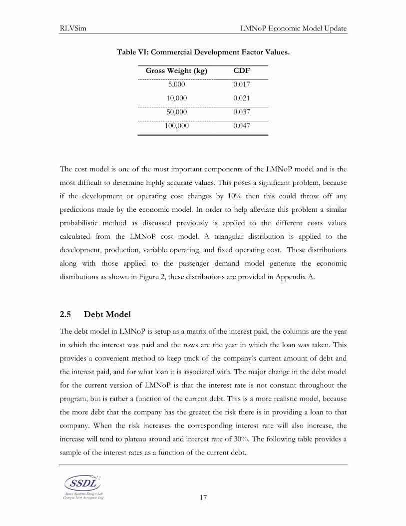
Table VI: Commercial Development Factor Values.
Gross Weight (kg) CDF
5,000 0.017
10,000 0.021
50,000 0.037
100,000 0.047
The cost model is one of the most important components of the LMNoP model and is the
most difficult to determine highly accurate values. This poses a significant problem, because
if the development or operating cost changes by 10% then this could throw off any
predictions made by the economic model. In order to help alleviate this problem a similar
probabilistic method as discussed previously is applied to the different costs values
calculated from the LMNoP cost model. A triangular distribution is applied to the
development, production, variable operating, and fixed operating cost. These distributions
along with those applied to the passenger demand model generate the economic
distributions as shown in Figure 2, these distributions are provided in Appendix A.
2.5 Debt Model
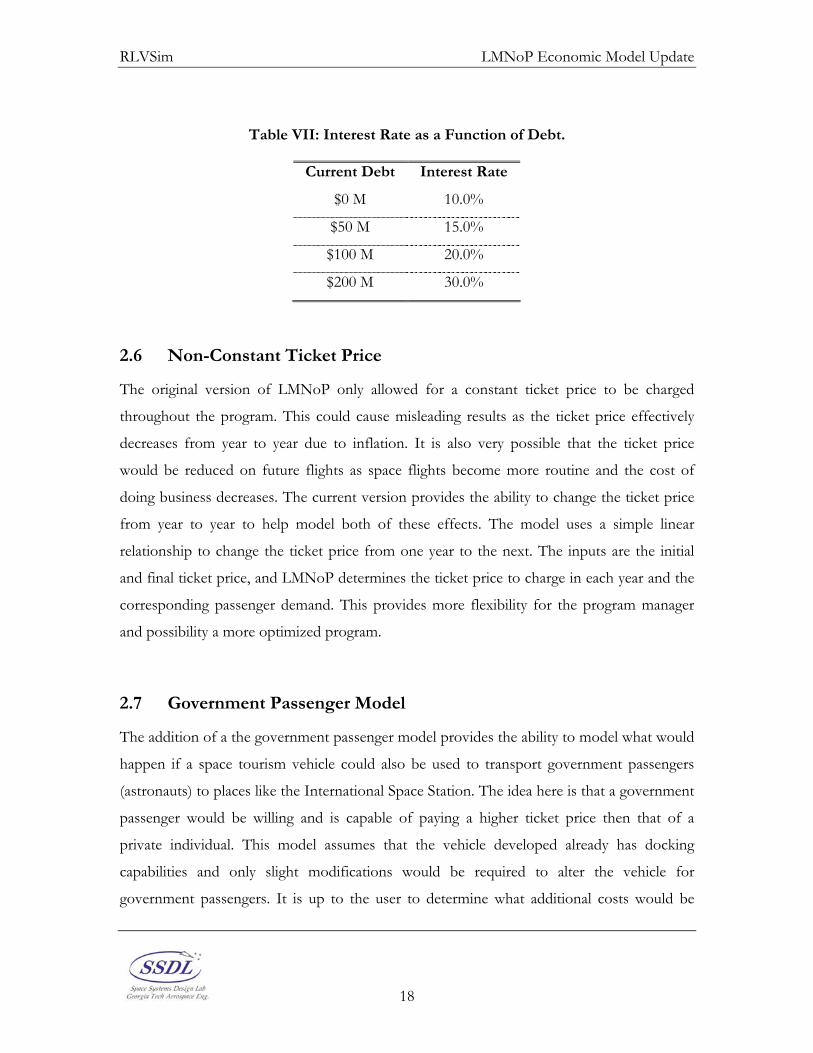
The debt model in LMNoP is setup as a matrix of the interest paid, the columns are the year
in which the interest was paid and the rows are the year in which the loan was taken. This
provides a convenient method to keep track of the company’s current amount of debt and
the interest paid, and for what loan it is associated with. The major change in the debt model
for the current version of LMNoP is that the interest rate is not constant throughout the
program, but is rather a function of the current debt. This is a more realistic model, because
the more debt that the company has the greater the risk there is in providing a loan to that
company. When the risk increases the corresponding interest rate will also increase, the
increase will tend to plateau around and interest rate of 30%. The following table provides a
sample of the interest rates as a function of the current debt.
17
RLVSim LMNoP Economic Model Update
Table VII: Interest Rate as a Function of Debt.
Current Debt Interest Rate
$0 M 10.0%
$50 M 15.0%
$100 M 20.0%
$200 M 30.0%
2.6 Non-Constant Ticket Price
The original version of LMNoP only allowed for a constant ticket price to be charged
throughout the program. This could cause misleading results as the ticket price effectively
decreases from year to year due to inflation. It is also very possible that the ticket price
would be reduced on future flights as space flights become more routine and the cost of
doing business decreases. The current version provides the ability to change the ticket price
from year to year to help model both of these effects. The model uses a simple linear
relationship to change the ticket price from one year to the next. The inputs are the initial
and final ticket price, and LMNoP determines the ticket price to charge in each year and the
corresponding passenger demand. This provides more flexibility for the program manager
and possibility a more optimized program.
2.7 Government Passenger Model
The addition of a the government passenger model provides the ability to model what would
happen if a space tourism vehicle could also be used to transport government passengers
(astronauts) to places like the International Space Station. The idea here is that a government
passenger would be willing and is capable of paying a higher ticket price then that of a
private individual. This model assumes that the vehicle developed already has docking
capabilities and only slight modifications would be required to alter the vehicle for
government passengers. It is up to the user to determine what additional costs would be
18

RLVSim LMNoP Economic Model Update
required to upgrade the vehicle to accommodate government passengers, these cost are built
into the model. The model assumes that NASA would just purchase a flight like any other
customer, except that they would likely purchase all of the seats on a particular flight and just
use the remainder of the vehicle capacity to transfer supplies. The government launch price
curve was taken from the Cost and Business Analysis Module (CABAM) developed by the
Space Systems Design Lab and derived from the Commercial Space Transportation Study
predictions. The Launch price per available seat is shown in Table VIII for a range of
required yearly launches. These prices are close to three times higher then the ticket price
expected to be charged to private individuals, yet they are remarkably lower then what
current estimates predict for the return of the Space Shuttle in 2005.
Table VIII: Government Launch Price.
Annual Government Launches Launch Price ($M)
1 $35 M/Seat
2 $33 M/Seat
3 $31 M/Seat
4 $29 M/Seat
5 $27 M/Seat
6 $25 M/Seat
A further investigation will be preformed to see how the addition of government passengers
effects the economic model of a space tourism docking mission. It looks like this would be a
real benefit to both NASA and the space tourism operator if a vehicle can be developed to
accommodate the needs and requirements of both.
19

RLVSim Space Tourism Market Analysis Using LMNoP
3.0 Space Tourism Market Analysis Using LMNoP
The second part of this project is to investigate the economic viability of the space tourism
industry. This includes a look into both the sub-orbital and orbital markets. The goals of this
study will be to determine the optimized characteristics of a space tourism program. This
optimization will be done for two different philosophies associated with the space tourism
industry. The first philosophy states that a company capable of providing space tourism
flights would do so in an attempt to generate a maximum profit for the company. This
means that a company is more interested in an optimized economic scenario than they are in
providing access to space for the general public. The second philosophy states that a
company is more interested in providing a greater good to the general public than
maximizing their return. This company is interested in maximizing the number of passengers
flown while maintaining a minimum profit. The optimized program for these two
philosophies is expected to differ substantially. The characteristics (LMNoP Inputs) of the
space tourism program under consideration are the following:
1. Vehicle’s Passenger Capacity – This will affect the overall size of the vehicle and
therefore the initial development cost.
2. Fleet Size – This will effect the number of possible flights per year and the total size
of the initial investments.
3. Length of the program – How many years the vehicle will operate.
4. Initial Ticket Price – Establishes the number of annual passengers.
These four characteristics provide the ability to setup a program cash flow and determine its
economic viability. This will assume that the other vehicle factors such as turn around time
and reliability, and the economic factors such as interest, inflation and discount rates remain
constant among the different programs. A list of these values is provided in Table IX.
20
RLVSim Space Tourism Market Analysis Using LMNoP
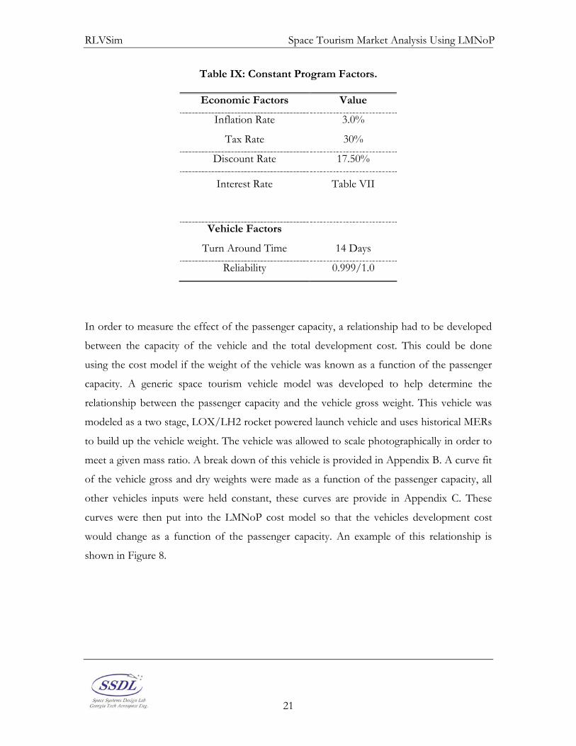
Table IX: Constant Program Factors.
Economic Factors Value
Inflation Rate 3.0%
Tax Rate 30%
Discount Rate 17.50%
Interest Rate Table VII
Vehicle Factors
Turn Around Time 14 Days
Reliability 0.999/1.0
In order to measure the effect of the passenger capacity, a relationship had to be developed
between the capacity of the vehicle and the total development cost. This could be done
using the cost model if the weight of the vehicle was known as a function of the passenger
capacity. A generic space tourism vehicle model was developed to help determine the
relationship between the passenger capacity and the vehicle gross weight. This vehicle was
modeled as a two stage, LOX/LH2 rocket powered launch vehicle and uses historical MERs
to build up the vehicle weight. The vehicle was allowed to scale photographically in order to
meet a given mass ratio. A break down of this vehicle is provided in Appendix B. A curve fit
of the vehicle gross and dry weights were made as a function of the passenger capacity, all
other vehicles inputs were held constant, these curves are provide in Appendix C. These
curves were then put into the LMNoP cost model so that the vehicles development cost
would change as a function of the passenger capacity. An example of this relationship is
shown in Figure 8.
21

RLVSim Space Tourism Market Analysis Using LMNoP
34.00
34.50
35.00
35.50
36.00
36.50
37.00
37.50
0 2 4 6 8 10 12 14 1
Passenger Capacity
Cos
t to
Firs
t Veh
cile
($M
6
)
Figure 8: Sub-Orbital Cost to First Vehicle as a Function of Capacity.
In order to determine the set of characteristics that optimize the two philosophies disused
earlier an optimization scheme needed to be employed. The two options considered were a
Genetic Algorithm and a Full Grid Search. Both of these methods would be able to handle
discrete and integer values. The full grid search would look at every possible combination of
the four characteristics listed above; this was initially estimated to be 6,160 combinations.
The GA would likely decrease the number of runs to fewer than 2,000. Since each of the
simulations is run probabilistically and require approximately 5 seconds to complete the GA
provides the possibility of six hours of time savings. The problem that was encountered
when running the simulations is that the results could vary from one run to the next, due to
the stochastic nature of the problem. In addition to this a certain set of combinations
resulted in very similar objective functions, results that different by less then 5%. In general
there were a collection of results that were within a few percent of the best objective
function. It was difficult to determine if the GA correctly considered the entire design space
and where or not it look at all the possible configurations that were within this small
percentage of the optimal design. It was therefore decided that a grid search would provide a
more complete look at the entire design space. It would require a longer run time, but once
22

RLVSim Space Tourism Market Analysis Using LMNoP
it was complete the entire design space would be available and a ranking of the top choices
could be made. In order to decrease the run time a smaller ranges were used for each of the
design variables. The final ranges investigated are shown in Table X and represent about
1,500 combinations.
Table X: Ranges Used for Program Factors.
Capacity Program Length (yr) # of Vehicles Ticket Price ($M)
Sub-Orbital
Max: Net Present Value 5 – 10 5 – 12: R = 0.999
12: R = 1.0 1 – 5 0.6 – 1.0
Max: Total Passengers 5 – 10 5 – 12: R = 0.999
12: R = 1.0 1 – 5 0.1 – 0.5
Orbital
Max: Net Present Value 8 – 15 5 – 12: R = 0.999
12: R = 1.0 1 – 5 8 – 15
Max: Total Passengers 8 – 15 5 – 12: R = 0.999
12: R = 1.0 1 – 5 1 – 5
The following sections will discuss in detail the results of this study and how they compare
to current space tourism programs. The following sections will look at the Virgin Galactic
model as it is currently advertised, possible improvements that could be made to this model,
effects of changing passenger demand on the Virgin Galactic model, and finally a general
optimized sub-orbital and orbital space tourism market.
23

RLVSim Virgin Galactic and SpaceShipTwo Market Study
4.0 Virgin Galactic and SpaceShipTwo Market Study
Virgin Galactic will become the first commercial space tourism company to provide sub-
orbital space flights when it begins operations in 2007 [10]. Virgin Galactic will operate a
derivative of the historic SpaceShipOne. This vehicle has been coined SpaceShipTwo. Very
little information is known about this vehicle, but what is known is that the vehicle will likely
be a scaled up version of SpaceShipOne carrying 5 – 8 passengers and traveling to an altitude
of 350,000 ft which should provide 7 – 10 minutes of weightlessness. Virgin Galactic has
purchased the rights to SpaceShipTwo and placed an order for five vehicles to be built by
2007. The Virgin Galactic model consist of a $125 M investment, which includes $100 M
paid to Scaled Composites for the development and production of five SpaceShipTwo
vehicles, and a $25 M facilities development cost. Virgin Galactic plans to sale 3,000 tickets
over 5 years of operation at a ticket price of $200,000. A summary of the Virgin Galactic
model is provided in Table XI.
Table XI: Virgin Galactic Model.
Passenger Capacity 5 - 8
Altitude(km) 350,000
Weightlessness (min) 7 - 10
Ticket Price ($) 200,000
Investment Cost ($M) 125
Operating Cost ($/Flight) 0.55*
IOC 2007
Operating Years 5
Passengers / Year 600
* Calculated from the LMNoP cost model not provided by Virgin Galactic
The Virgin Galactic Model as described above will be investigated using LMNoP in order to
determine the economic viability of the current program. The term “economic viability”
24

RLVSim Virgin Galactic and SpaceShipTwo Market Study
refers to the ability to meet specific economic requirements. In this case the requirement for
economic viability will be a net present value greater then zero. Slight changes needed to be
made to the LMNoP model in order to accurately model the Virgin Galactic program. The
most important was a increase in the market demand model that was needed to match the
600 passengers/year predicted by Virgin Galactic, this required a 3.1x multiplier on the
market model within LMNoP as it only predicted 967 passengers/year. The discrepancies
are large between the two models, this could be due to Virgin Galactic’s advertisement that it
will only operate for five years, this “limited time offer” would likely increase the demand as
people would be concerned about possibly missing their initial opportunity. There may also
be a push to be apart of the first group of space tourists, an excitement factor. This
investigation will be done stochastically using the input distribution provided in Appendix A
in order to provide a greater confidence in the results of this investigation; these results will
be provided at a 90% confidence.
The reliability of SpaceShipTwo is not known and so the investigation will look at two
possible cases in order to explore the sensitively to vehicle reliability. Case 1 will be a
perfectly reliable vehicle (R = 1.0), and Case 2 will be a vehicle with a 1/1000 chance of
failure (R=0.999). Case 1 will provide the best case scenario and Case 2 will provide insight
as to how reliability affects the economic viability of the design.
4.1 Case 1 - 100% Reliability, Virgin Galactic Passenger Model
Case 1 assumes that SpaceShipTwo has 100% reliability and completes all 600 flights without
incidence. This totals to 3,000 tickets over the course of five years for a total revenue of
$600 M. This generates a Net Present Value of $15.1 M which suggests that this case is an
economically viable program. In actuality there is a 100% chance that if there are no failures
over the five years of operation that the Virgin Galactic program will be economically viable.
Even for the worse set of noise variable, the highest development and operating cost, the
program would still see an NPV of $7.5 M. This suggests that the program is very robust, as
long as no failures occur. The probability density function (PDF) for the NPV is shown in
Figure 9, the blue section is 90% confidence interval.
25

RLVSim Virgin Galactic and SpaceShipTwo Market Study
Frequency Chart
Certainty is 90.00% from $15.07 to $32.50
.000
.008
.015
.023
.030
0
7.5
15
22.5
30
$7.50 $13.75 $20.00 $26.25 $32.50
1,000 Trials 999 Displayed
Forecast: NPV
Frequency Chart
Certainty is 90.00% from $15.07 to $32.50
.000
.008
.015
.023
.030
0
7.5
15
22.5
30
$7.50 $13.75 $20.00 $26.25 $32.50
1,000 Trials 999 Displayed
Forecast: NPV
Figure 9: Virgin Galactic Results for R = 1.0.
The NPV evaluation helps to determine if an investment should be undertaken and is a good
method to compare different investment options. It general it is difficult to understand what
a NPV of 15.7 $M represents in terms of a cash flow, therefore it will be useful to look at
the total profit, return on investment (ROI), and expect revenue for each program. The total
profit is the final cash on hand at the end of the program after all expenditures have been
paid, the ROI is the incremental gain divided by the total investment cost, and the revenue is
the total amount of money generated.
100
Rex
CostTotal
CostTotalvenueROI
⎟⎠⎞⎜
⎝⎛ −
= (6)
There is a 90% confidence that the Virgin Galactic model will generate at least a 16.9% ROI
and a total profit of $81.6 M (FY 2005). These distributions are shown in Figure 10 below. A
final profit of $81.6 M is small considering the size of the initial investment and the risk that
is involved in operating a space tourism vehicle. A single failure could drastically effect the
economic viability of this program. This effect will be looked at closer in next section. It is
likely that there are other factors involved in Virgin Galactic’s decision that are not
26

RLVSim Virgin Galactic and SpaceShipTwo Market Study
addressed in this study, it seems that there is possibly a better solution to the sub-orbital
space tourism model than one with such a small return.
Frequency Chart
Certainty is 90.00% from 81.58 to 130.00
.000
.007
.014
.020
.027
0
6.75
13.5
20.25
27
60.00 77.50 95.00 112.50 130.00
1,000 Trials 998 Displayed
Forecast: End Cash
Frequency Chart
Certainty is 90.00% from 16.94% to 27.50%
.000
.008
.016
.024
.032
0
8
16
24
32
12.50% 16.25% 20.00% 23.75% 27.50%
1,000 Trials 998 Displayed
Forecast: ROI
Frequency Chart
Certainty is 90.00% from 81.58 to 130.00
.000
.007
.014
.020
.027
0
6.75
13.5
20.25
27
60.00 77.50 95.00 112.50 130.00
1,000 Trials 998 Displayed
Forecast: End Cash
Frequency Chart
Certainty is 90.00% from 16.94% to 27.50%
.000
.008
.016
.024
.032
0
8
16
24
32
12.50% 16.25% 20.00% 23.75% 27.50%
1,000 Trials 998 Displayed
Forecast: ROI
Figure 10: Virgin Galactic Results for R = 1.0 (Total Profit, ROI).
The yearly and cumulative cash flows are shown in Figure 11, these values are discounted at
17.5 % and presented in FY $2005. The initial investment is spread over the first three years
while vehicles are being developed and built by Scaled Composites. Operations begin in year
2007 and last until 2011, the revenue and cost for these five years is the same, and the drop
off that is seen is due to the inflation rate. The cumulative cash flow experiences a large drop
due to the initial investment at the beginning of the program and then begins to rise once
operations begin. The program breaks even somewhere between 2008 and 2009.
$(150)
$(100)
$(50)
$-
$50
$100
$150
2003 2004 2005 2006 2007 2008 2009 2010 2011
$M F
Y20
04
Yearly Cash FlowCummulative Cash Flow
Figure 11: Virgin Galactic Discounted Cash Flow Analysis, No Failure (FY $2004).
27

RLVSim Virgin Galactic and SpaceShipTwo Market Study
4.2 Case 2 – 1/1000 Chance of Failure, Virgin Galactic Model
The second study of the Virgin Galactic model assumes that the vehicle reliability does not
have a 100% reliability and that the vehicles will fail 1/1000 times. This equates to a
reliability of R = 0.999. The Virgin Galactic model assumes about 600 flights over the life of
the program so it is not expected to see a crash during every simulation. The total number of
failures that occur during the 1,000 simulations is provided in Table XII. A failure occurs in
about 40% of the simulations, when this occurs the reliability model begins to take effect.
These effects include a complete loss of the market for the failure year, as the vehicle is
being overhauled to determine the cause of failure. The years following the failure
experience a decreased in demand as the market is regaining confidence in the vehicle, this
recovery trend can be seen in Figure 4 and Figure 5 . There is also an insurance premium
that must be paid along with legal fees and any cost associated with recertifying the fleet for
flight. This could potentially be a large cost to the space tourism operator, especially the first
time that it occurs. This could be in the neighborhood of $50 - $100 M.
Table XII: Failure Record for R = 0.999.
Failures Frequency
0 568
1 342
2 90
This failure has a drastic effect on the economic viability of the program. In the initial case
there was a 100% chance of obtaining a NPV greater than zero, in this case there is only a
55% certainty in reaching this value. That is a very low probability of success and it is
unlikely that the project would be successful. The NPV resulting for this simulation is shown
in Figure 12. This result tends to show a multi-modal tendency where both the failure and
non-failure cases exhibit a normal distribution. The reason behind such a low chance of
success is due to this multi-modal effect. The cases where there is a failure, either one or two
28

RLVSim Virgin Galactic and SpaceShipTwo Market Study
failures, the NPV is less than zero, and this pulls the confidence level down because there is
such a large percentage of the cases where the program isn’t viable. The cause of this is that
the number of passengers decreases so greatly in the cases where there is a failure that
enough revenue can not be generated to offset the initial investment cost.
Frequency Chart
Certainty is 90.00% from ($75.92) to $50.00
.000
.019
.039
.058
.078
0
19.25
38.5
57.75
77
($100.00) ($62.50) ($25.00) $12.50 $50.00
991 Trials 991 Displayed
Forecast: NPV
Frequency Chart
Certainty is 90.00% from 1,735.00 to 3,250.00
.000
.013
.025
.038
.050
0
12.5
25
37.5
50
500.00 1,187.50 1,875.00 2,562.50 3,250.00
1,000 Trials 982 Displayed
Forecast: Total Number of Passengers
Frequency Chart
Certainty is 90.00% from ($75.92) to $50.00
.000
.019
.039
.058
.078
0
19.25
38.5
57.75
77
($100.00) ($62.50) ($25.00) $12.50 $50.00
991 Trials 991 Displayed
Forecast: NPV
Frequency Chart
Certainty is 90.00% from 1,735.00 to 3,250.00
.000
.013
.025
.038
.050
0
12.5
25
37.5
50
500.00 1,187.50 1,875.00 2,562.50 3,250.00
1,000 Trials 982 Displayed
Forecast: Total Number of Passengers
Figure 12: Virgin Galactic Results for R = 0.999 (NPV, Number Passengers).
The effect of the decrease in passengers is easily seen in Figure 13, in the cases where the
program experiences a failure the total profit and ROI are negative. This signifies that the
revenue generated was not enough to off set the total cost of the program. The 90%
confidence values do not have much meaning in this case because there is such a
discrepancy in the two cases. The importance of this study is that a vehicle failure is a very
important factor to the economic viability of the program. This effect can not be simply
ignored in the design of a successful project.
Frequency Chart
Certainty is 90.00% from -244.98 to 150.00
.000
.020
.039
.059
.079
0
19.5
39
58.5
78
-350.00 -225.00 -100.00 25.00 150.00
991 Trials 991 Displayed
Forecast: End Cash
Frequency Chart
Certainty is 90.00% from -40.22% to 30.00%
.000
.024
.048
.073
.097
0
24
48
72
96
-80.00% -52.50% -25.00% 2.50% 30.00%
991 Trials 991 Displayed
Forecast: ROI
Frequency Chart
Certainty is 90.00% from -244.98 to 150.00
.000
.020
.039
.059
.079
0
19.5
39
58.5
78
-350.00 -225.00 -100.00 25.00 150.00
991 Trials 991 Displayed
Forecast: End Cash
Frequency Chart
Certainty is 90.00% from -40.22% to 30.00%
.000
.024
.048
.073
.097
0
24
48
72
96
-80.00% -52.50% -25.00% 2.50% 30.00%
991 Trials 991 Displayed
Forecast: ROI
Figure 13: Virgin Galactic Results for R = 0.999 (ROI, Total Profit).
29

RLVSim Virgin Galactic and SpaceShipTwo Market Study
The cash flow analysis shown in Figure 14 is a representative look at the program life of the
Virgin Galactic model. In this case there is a single failure that occurs in the second year of
operations. The cash flow is very similar to Case 1 up through 2007, but with the failure in
2008 the program has a large expense that increases the debt to almost $100 M. This can not
be recouped in the remains years of the program, especially at the decreased market demand
that will be experienced in the following few years. It would take an additional five years of
operations in order to re-coup the cost of this failure. It could be suggested that if a failure
occurred Virgin Galactic would just end operations so that it didn’t incur this recertification
expense. Further study of the impact of this expense along with its magnitude should be
conducted.
$(100)
$(80)
$(60)
$(40)
$(20)
$-
$20
$40
2003 2004 2005 2006 2007 2008 2009 2010 2011
US
$M
Yearly Discounted Cash FlowCumm. Discounted Cash Flow
Figure 14: Virgin Galactic Cash Flow Analysis, 2009 Failure.
A summary of both cases are shown in Table XIII, note that the 90% confidence for Case 2
is only shown in order to provide a comparison to Case 1. The effect of a single vehicle
failure for the Virgin Galactic model would eliminate any chance of the program becoming
economically viable. The 0.999 reliability is very optimistic as a vehicle has never proven to
have a flight reliability this high. The vehicle reliability will be very important in the design of
a space tourism vehicle, and some time should be spent trying to understand the vehicle
30

RLVSim Virgin Galactic and SpaceShipTwo Market Study
reliability and how it can be improved. It is very likely that Richard Branson would be willing
to accept a program that wasn’t profitable in order to be become the first operating space
tourism company. It may be possible to re-design the Virgin Galactic model such that it has
the capability of withstanding a vehicle failure.
Table XIII: Virgin Galactic Summary of Results (90% Confidence).
R = 1.0 R = 0.999
Net Present Value ($M) 15.1 -75.9
Return on Investment (%) 16.9 -40.2
Ending Cash ($M) 81.6 -244.9
Number of Passengers 2,830 1,735
4.3 Virgin Galactic Study of Alternatives
This study will attempt to increase the robustness of the Virgin Galactic program such that it
could withstand a possible failure and remain an economically viable program. In order to
keep the baseline Virgin Galactic model, the passenger demand multiplier remained on the
LMNoP market data so that the Virgin Galactic demand estimations could be used. Only the
vehicle passenger capacity, ticket price and operating time frame were altered for this study.
The initial investment of $125 M was also kept constant. The following set of trade studies
should help establish trends in the market and provide some information on where a more
optimized solution may exist.
4.3.1 Virgin Galactic Ticket Price Sweep, 5 passengers The first trade study was to look at how the ticket price affected the outlook of the market.
The ticket price was run from $0.1 – $1.0 M holding the other components of the Virgin
Galactic model constant, except that the passenger demand was allowed to change according
to the ticket price. The results for the NPV and the number of passengers as a function of
31

RLVSim Virgin Galactic and SpaceShipTwo Market Study
the ticket price are shown in Figure 15, the $0.2 M point corresponds to the original Virgin
Galactic model. The increase in ticket price, as expected, has a negative effect on the
number of passengers willing to pay that price. There is a significant decrease in the total
number of passengers, dropping from over 3,000 at a ticket price of $0.1 M to 600 for a $1.0
M ticket price. This actually has a very large positive effect on the NPV of the program. The
case where the reliability was assumed to be 100% has a maximum NPV of over $150 M at a
ticket price around $0.9 M, that is a 10x increase from the baseline Virgin Galactic model.
The case where there is a 1/1000 chance of failure reaches a NPV greater than zero when
the ticket price is increased above $0.6 M. This indicates that there is a program design that
is robust enough to withstand a loss of vehicle.
($150.00)
($100.00)
($50.00)
$0.00
$50.00
$100.00
$150.00
$200.00
0.0 0.2 0.4 0.6 0.8 1.0 1.2
Ticket Price ($M)
Net
Pre
sent
Val
ue ($
M)
R = 1.0
R = 0.9990
500
1000
1500
2000
2500
3000
3500
0.0 0.2 0.4 0.6 0.8 1.0 1.2
Ticket Price ($M)
Num
ber o
f Pas
seng
ers R = 1.0
R = 0.999
($150.00)
($100.00)
($50.00)
$0.00
$50.00
$100.00
$150.00
$200.00
0.0 0.2 0.4 0.6 0.8 1.0 1.2
Ticket Price ($M)
Net
Pre
sent
Val
ue ($
M)
R = 1.0
R = 0.9990
500
1000
1500
2000
2500
3000
3500
0.0 0.2 0.4 0.6 0.8 1.0 1.2
Ticket Price ($M)
Num
ber o
f Pas
seng
ers R = 1.0
R = 0.999
* Calibrated for Virgin Galactic Market Model
Figure 15: Virgin Galactic Ticket Price Trade Study (5 Pax).
There are two important reasons why the NPV has such a positive correlation with an
increase in the ticket price. The first and most important is that the increase in passenger
revenue is larger then the decrease in passenger demand so the effect is a net increase in the
total revenue generated each year. This tends to peak around a ticket price of $0.9 M where
the percentage increase in ticket price becomes small. The second factor only affects the
cases where reliability is added to the problem because a decrease in the number of
passengers reduces the number of required flights which decreases the likelihood of a vehicle
failure. This will force the case with reliability added to approach the 100% reliable case, this
can be seen more clearly in Figure 18.
32

RLVSim Virgin Galactic and SpaceShipTwo Market Study
4.3.2 Virgin Galactic Ticket Price Sweep, 8 passengers
The second trade study was to look at how an eight passenger capacity vehicle would
compare to that of the five passenger vehicle. The initial investment cost will remain $125
M, the effect of changing passenger capacity on the vehicle size and the total investment cost
will be included in later studies. The eight passenger case is presented in Figure 16 and
shows very similar results to that of the five passenger case. The NPV still peaks around $0.9
M, but the curves are shifted toward the left. This means that Case 2 now has a positive
NPV for a ticket price greater then $0.4 M, $0.2 M less than that for the five passenger
vehicles. That is a very large increase for only three additional passengers. The coupling of
both an increase in the passenger capacity with the increase in ticket price allows the number
of passengers for Case 2 to approach the 100 % reliability case at a much faster rate. This is
again due to a decrease in the chance of failure associated with a decrease in the total
number of flights.
($150.00)
($100.00)
($50.00)
$0.00
$50.00
$100.00
$150.00
$200.00
0 0.2 0.4 0.6 0.8 1 1.2
Ticket Price ($M)
Net
Pre
sent
Val
ue
R = 1.0
R = 0.9990
500
1000
1500
2000
2500
3000
3500
4000
4500
5000
0 0.2 0.4 0.6 0.8 1 1.2
Ticket Price ($M)
Num
ber o
f Pas
seng
ers
R = 1.0
R = 0.999
($150.00)
($100.00)
($50.00)
$0.00
$50.00
$100.00
$150.00
$200.00
0 0.2 0.4 0.6 0.8 1 1.2
Ticket Price ($M)
Net
Pre
sent
Val
ue
R = 1.0
R = 0.9990
500
1000
1500
2000
2500
3000
3500
4000
4500
5000
0 0.2 0.4 0.6 0.8 1 1.2
Ticket Price ($M)
Num
ber o
f Pas
seng
ers
R = 1.0
R = 0.999
Figure 16: Virgin Galactic Ticket Price Trade Study (8 Pax).
4.3.3 Virgin Galactic Program Length Sweep, 5 passengers The trade study was to look at how the operating length of the program would affect the
economic viability. The ticket price was set at $0.2 M, the passenger capacity was set to five
and the yearly passenger demand was set to match what was predicted by the Virgin Galactic
model. The effect of increasing the program length from 4 – 14 years is shown in Figure 17.
33

RLVSim Virgin Galactic and SpaceShipTwo Market Study
The results of the 100% reliable case are as expected, since there are no losses associated
with an increase in the length of the program the number of passengers and NPV both
increase with an increase in operating years. This is the ideal case, it reality an increase in the
number of years that the vehicle operate greatly increases the chance of failure. This is seen
in Case 2 where there isn’t a simple linear increase in the passenger demand. There is an
unexpected maximum in the total number of passengers. At some point the increase in
number of flights becomes high enough as to ensure a failure at some point in the program.
At this point the total number of passengers drops off and remains relatively constant for
any increase in program length. This could be offset by an increase in the passenger capacity
and/or ticket price which would help to decrease the number of flights.
0
1000
2000
3000
4000
5000
6000
7000
8000
9000
4 6 8 10 12 14 16
Program Operating Years
Num
ber o
f Pas
seng
ers
R = 0.999
R = 1.0
Figure 17: Virgin Galactic Operating Years Trade Study (5 Pax) 90% Confidence.
4.3.4 Virgin Galactic Program with Futron Data, Ticket Price Sweep
One of the major concerns with the Virgin Galactic market model is that it predicts a much
larger passenger demand than any of the currently available models. It predicts 3x as many
passengers as the LMNoP model at any given ticket price. Some of this was explained to be
a result of the program only operating for five years, at which time there may or may not be
another program available. However, it would be of interest to see how economically viable
the Virgin Galactic model is if it used the LMNoP market demand model. These results are
34

RLVSim Virgin Galactic and SpaceShipTwo Market Study
shown in Figure 18. The results of this study do not look very promising. There is only a
small range of ticket prices that provide a positive NPV solution. Looking at the original
Virgin Galactic ticket price (TP = $0.2 M) even the 100% reliable vehicle can not generate a
positive NPV (NPV = -40 $M). The asymptotical trend of Case 2 is greatly exaggerated and
nearly match the 100% reliable case for a ticket price greater then $0.6 M. For this low
passenger demand case the vehicle’s reliability doesn’t have as large of an effect on the
design of the vehicle program. By the time that the program has become viable the two
curves overlap. These results should cause some concern for the viability of the Virgin
Galactic model. If it doesn’t get the passenger demand that it predicts, it will be very tough
for the program to remain viable at the current ticket price.
0
200
400
600
800
1000
1200
1400
1600
0 0.2 0.4 0.6 0.8 1 1.2
Ticket Price ($M)
Net
Pre
sent
Val
ue ($
M)
($140.00)
($120.00)
($100.00)
($80.00)
($60.00)
($40.00)
($20.00)
$0.00
$20.00
Num
ber o
f Pas
seng
ers
R = 1.0
R = 0.999
R = 1.0
R = 0.999
Figure 18: Virgin Galactic Ticket Price Trade Study (Futron Market Data).
These trade studies provided evidence that the Virgin Galactic model could be optimized to
either improve upon the NPV or the total number of passengers that it services. The three
lessons learned from these trade studies are the ticket price that could be charged, this will
decrease the number of passengers, but at the same time greatly improve the economic
viability, especially for the case where reliability is brought into the problem. The vehicle
capacity seems to benefit the NPV of the program by increasing the revenue per flight
35
RLVSim Virgin Galactic and SpaceShipTwo Market Study
without greatly increasing the recurring cost, this study was done assuming that an increase
in the passenger capacity didn’t increase the development cost. In actuality this would not be
the case, for future studies the investment cost needs to be a function of the passenger
capacity. The capacity also helps decrease the chance of failure because fewer flights are
needed to meet the passenger demand. The program length had an unusual effect on the
case where reliability was included. It would be interesting to see if an increase in the
program length coupled with the other two factors could provide for a more optimized
vehicle program. The Virgin Galactic model will be the first program to provide space access
to the general public and in that it is truly revolutionary; however, it has much room for
improvement is the overall design of the program. The next section will outline a study that
could be used to guide the development of a more optimized and robust space tourism
program.
36

RLVSim Sub-Orbital Space Tourism Market Study
5.0 Sub-Orbital Space Tourism Market Study
The sub-orbital space tourism market study will attempt to develop an understanding of
what factors affect the design of a space tourism program. The factors under investigation
are the same three from the trade studies done on the Virgin Galactic model, ticket price,
passenger capacity, and program length in addition to fleet size. These factors were discussed
in detail previously and are shown in Table X along with their specified ranges. The goal of
the study will be to establish what combination of these factors optimizes the space tourism
program. Recall that an optimized space tourism market considers two different
philosophies, one is to maximize the net present value and the overall economic viability,
and the second is to provide the maximum number of passengers access to space while
maintaining a small profit. Both of these philosophies will be considered and a comparison
of the two will be made to see what similarities and differences exist. Two studies that will be
presented in this section. The first will be to determine what combination of ticket price,
passenger capacity and fleet size will comprise the most optimized program while keeping
the Virgin Galactic passenger demand model. This is being done so that a fair comparison
can be made between the results of this study and the Virgin Galactic model. The
standardized passenger model will provide a common platform to the compare the two
results. The second study will differ from the first in that it will use the entire LMNoP model
including the passenger demand curve, and the market expansion This will give the
optimization more freedom as the length of the program will be included as a design
variable. The hope here is that there is an optimal program length that balances the chance
of failure with the total capability of the program.
The results of this study will be to help to guide the design of a new space tourism program.
The results are not meant to be concrete, but rather as basic rules of thumb. It will be shown
that there are many possible solutions to this problem, but these solutions tend to
congregate in specific sections of the design space. It is these design sections that will be of
interest in determining an optimally design program.
37

RLVSim Sub-Orbital Space Tourism Market Study
5.1 Simulation Environment and Setup
The ModelCenter® environment was use to simplify the interface between the optimizer
and the LMNoP model. Crystal Ball was used for the Monte Carlo simulations from within
the LMNoP model. This was done to help increase the speed of simulation, the less
information that needs to be passed between models within ModelCenter the faster it will
run. A snap shot of the ModelCenter environment is shown in Figure 19.
Figure 19: ModelCenter Optimization Environment
The Monte Carlo analysis is built into the LMNoP model and uses a VBA script to
implement the simulation from within ModelCenter. Each simulation consists of 100
probabilistic simulations and 90% confidence value is taken from these results. An initial
comparison was done between 100 and 1,000 simulations and only a small difference was
seen in the 90% confidence value and so 100 simulation was used to help decrease the run
time, each set of 100 simulations takes approximately 5 seconds to complete. The
optimizers under consideration for this simulation were a Genetic Algorithm and a Full
Factorial Grid Search. The Genetic Algorithm has the ability to handle integer design
variables and in general can help to reduce the number of total function calls required for
large problems. The main concern when using a Genetic Algorithm is that it uses random
number generation when it moves through the design space and so is not guaranteed to find
the optimal solution. In general the Genetic Algorithm should be run many times from
38

RLVSim Sub-Orbital Space Tourism Market Study
different initial populations to confirm the results. Initially the Genetic Algorithm was used
in this simulation, but after running the results multiple times it was clear that the optimizer
would not be able to repeat the optimal value as it would change from one simulation to the
next due to the of the stochastic nature of the simulation. There are a series of program
configurations that are different in design but have very similar economic outputs. It was
impossible to determine if the GA looked at all of these cases. Since the design space tended
to have many similar solutions and the idea of this study was to find the target areas of the
design space then it would be more useful to be able to see the entire design space so that a
program designer would know where and where not to operate a program. Therefore it is
decided to go with the Full Factorial Grid Search over the Genetic Algorithm. Since the
probabilistic simulation only took a few seconds the Grid Search could be completed in a
reasonable amount of time (< 1hr) and then the entire design space would be known. This
would allow comparisons to be made between the different “optimal” designs and determine
if certain factors were insensitive to changes in a particular design variable. An example of
how the optimizers look at the different design spaces are provided in Figure 20 and Figure
21 , note just how many design points are very close to the actual optimal solution. The two
lines shown in Figure 20 are the current and best ever solutions.
Model.OptWorks GeneticAlgorithm.driverOutputs.bestValues.bestObjectiveFunctions
Run Number130120110100908070605040302010
0-10-20-30-40-50-60-70-80-90
-100-110-120-130-140-150-160-170-180-190-200-210-220-230-240-250-260-270-280-290
Net
Pre
sent
Val
ue
Run NumberModel.OptWorks GeneticAlgorithm.driverOutputs.bestValues.bestObjectiveFunctions
Run Number130120110100908070605040302010
0-10-20-30-40-50-60-70-80-90
-100-110-120-130-140-150-160-170-180-190-200-210-220-230-240-250-260-270-280-290
Model.OptWorks GeneticAlgorithm.driverOutputs.bestValues.bestObjectiveFunctions
Run Number130120110100908070605040302010
0-10-20-30-40-50-60-70-80-90
-100-110-120-130-140-150-160-170-180-190-200-210-220-230-240-250-260-270-280-290
Net
Pre
sent
Val
ue
Run Number
Figure 20: Space Tourism Design Space (Genetic Algorithm).
39

RLVSim Sub-Orbital Space Tourism Market Study
Run Number1101051009590858075706560555045403530252015105
-10
-20
-30
-40
-50
-60
-70
-80
-90
-100
-110
-120
-130
-140
-150
-160
-170
-180
-190
Net
Pre
sent
Val
ue
Run NumberRun Number
1101051009590858075706560555045403530252015105
-10
-20
-30
-40
-50
-60
-70
-80
-90
-100
-110
-120
-130
-140
-150
-160
-170
-180
-190
Run Number1101051009590858075706560555045403530252015105
-10
-20
-30
-40
-50
-60
-70
-80
-90
-100
-110
-120
-130
-140
-150
-160
-170
-180
-190
Net
Pre
sent
Val
ue
Run Number Figure 21: Space Tourism Design Space (Grid Search).
5.2 Market Optimization Using Virgin Galactic Market Model
5.2.1 Maximum Net Present Value Optimization (Virgin Galactic) The maximum NPV solution was once again calculated for both a 100% reliable vehicle and
for a vehicle with a 1/1000 chance of failure. The top four solutions for an R = 1.0 are
shown in Table XIV. These four solutions have a NPV that is slightly greater than $186 M
and total profit of about $480 M discounted to 2005 dollars. The total profit is the amount
of money on hand at the end of the program after all expenses have been paid These are
both much improved over the original Virgin Galactic model. There are two important
trends that can be seen in these results. The first is that in order to optimize the NPV, the
program would like to set the ticket price around $0.9 M. This is due to a greater increase in
profit per flight than is lost due to the drop off in demand at the higher ticket prices. This
effect tends to tail off at this ticket price, where the drop in demand becomes to great. The
second trend to note is that the optimized solution wants to build only a single vehicle with a
large passenger capacity. The program only needs a single vehicle to complete all of its
missions (TAT = 14 days) especially for the small number of passengers expected. The
greater passenger capacity provides greater revenue per flight without a proportional increase
in the operating cost of the vehicle.
40

RLVSim Sub-Orbital Space Tourism Market Study
Table XIV: Maximize NPV, R = 1.0.
Result 1 Result 2 Result 3 Result 4 Pass Capacity 10 9 9 8 Initial Ticket Price ($M) 0.9 0.85 0.9 1 Number Vehicles 1 1 1 1 Program Length (yr) 5 5 5 5 NPV ($M) 186 184 183 181 Number Passengers 1060 1134 1053 936 Total Profit ($M) 482 477 474 470
A very similar trend is seen in the case where a reliability of 0.999 is used, Table XV. The
NPV is still around $180 M with a total profit of about $460 M. The differences here in
these top results are likely due to the variations in the Monte Carlo simulations and not
actual different optimal design points. This case tends to approach the 100% reliable case
discussed above because at the high ticket price such that the market demand has decreased
to a level where the chance of failure is very small and the design is no longer dependent on
the reliability of the vehicle.
Table XV: Maximize NPV, R = 0.999.
Result 1 Result 2 Result 3 Result 4 Pass Capacity 10 10 8 9 Initial Ticket Price ($M) 1 0.85 0.9 1 Number Vehicles 1 1 1 1 Program Length (yr) 5 5 5 5 NPV ($M) 180 178 177 173 Number Passengers 930 1090 1032 612 Total Profit ($M) 467 461 458 448
A comparison between Result 1 and the Virgin Galactic model is shown in Figure 22, the
bar chart on the left includes the design variables while the chart on the right has the
economic outputs (NPV, Number of Passengers, and Total Profit). There is a very large
increase in both the NPV going from $15.7 M to $186 M and the total profit going from $82
M to $482 M. These are simply accomplished by increasing the ticket price, increasing the
41

RLVSim Sub-Orbital Space Tourism Market Study
fleet size and the passenger capacity of the vehicle. These are design changes that could
easily be implemented into a new program, so it begs the question as to why the program
was designed so differently. This questioned will be answered in the next study.
10
4
0.2
4
10.9
55
0
2
4
6
8
10
12
Pass Capacity Initial Ticket Price Number Vehciles Program Length
Improved Virgin GalacticVirgin Galactic
1060
482
15
2880
82186
0
500
1000
1500
2000
2500
3000
3500
NPV Number Passengers Total Profit
Improved Virgin GalacticVirgin Galactic
Figure 22: Virgin Galactic Demand Model Comparison (Max NPV).
5.2.2 Maximum Number of Passenger Optimization (Virgin Galactic) The second study in this section looks at how to optimize a space tourism program in order
to maximum the actual number of passengers. This goes along with the second philosophy,
that the goal of a space tourism program is to provide a service to humanity and creating an
economically viable program is only a minimum requirement and not the main objective
function. The first of these results, the case where the reliability is 100%, is provided in
Table XVI. These results are vastly different than the ones seen for the maximum NPV
cases discussed above. The major difference to note is that the ticket price has dropped
dramatically as would be expected knowing the correlation of ticket price and market
demand. The ticket price however didn’t reach the minimum allowable ticket price of $0.1 M
because at this price the program isn’t economically viable and so even though the number
of passengers was greater, a program couldn’t operate in this region and so these cases were
discarded. The $0.2 M was the minimum ticket price for which a NPV of greater than zero
could be obtained. The passenger capacity still tends to be high because this allows more
revenue to be generated for each, this allows for a lower ticket price to be charged and a
corresponding increase in the passenger demand. The fleet size is larger than the previous
case because a single vehicle does not have enough capability, even at the high capacities.
The optimal number of passengers requires at least three vehicles (9 Passengers) to meet the
2,850 passenger requirement over a five year program with an assumed turn around time of
42

RLVSim Sub-Orbital Space Tourism Market Study
14 days. These design variables correspond to a NPV between $25 – $40 M and a total profit
of $100 M.
Table XVI: Maximize Number of Passengers, R = 1.0.
Result 1 Result 2 Result 3 Result 4 Pass Capacity 7 9 9 10 Initial Ticket Price ($M) 0.2 0.2 0.2 0.2 Number Vehicles 4 3 5 3 Program Length (yr) 5 5 5 5 NPV ($M) 26 38 28 39 Number Passengers 2856 2844 2844 2840 Total Profit ($M) 98 127 109 130
In this optimization problem the solution is a function of the vehicle reliability and some
differences will exist in the program design variables between these two scenarios. The
reliability plays an important factor in this solution because the number of passengers is
directly related to the chance of vehicle failure. A high chance of failure will decrease the
economic viability of the program because of the large cost associated with the loss of a
vehicle along with the decrease in demand that would be seen following such a failure. The
solution counters this increased chance of failure by increasing the ticket price and
decreasing the number of passengers until the chance of failure decreases and the NPV
becomes greater than zero. This effect is shown in Figure 23 where the actual maximum
number of passengers occurs at a ticket price of 0.2 $M, but the cutoff for an economically
viable solution is at a ticket price of 0.35 $M. A ticket price of 0.2 $M corresponds to the
value obtained in 100 % reliable solutions because the NPV cutoff for this solution is less
then $0.2 M and so the solution can reach this peak.
43

RLVSim Sub-Orbital Space Tourism Market Study
Figure 23: Maximum Passenger Ticket Price Cutoff.
The top four solutions are shown in Table XVII. All of these solutions have a low NPV
around $10 M and total profit of about $50 M. If the resolution of the problem was
increased the solution would drive down the ticket price until the NPV = 0 or whatever
minimum level was set. The results are a ticket price of about $0.35 M and a fleet size of two
vehicles, which is capable of providing flights for over 1,300 passengers while maintaining an
economically viable program.
Table XVII: Maximize Number of Passengers, R = 0.999.
Result 1 Result 2 Result 3 Result 4 Pass Capacity 9 10 8 9 Initial Ticket Price ($M) 0.35 0.4 0.4 0.45 Number Vehicles 2 2 2 3 Program Length (yr) 5 5 5 5 NPV ($M) 8 17 15 12 Number Passengers 1,377 1,260 1,112 1,107 Total Profit ($M) 61 37 56 41
44

RLVSim Sub-Orbital Space Tourism Market Study
A comparison of the program design variables are provide in Figure 24. The results are
similar for both cases with the first case having a lower ticket price, about 50% less, and a
slightly large fleet size.
0.2
4
10
0.5
2
43
9
0
2
4
6
8
10
12
Pass Capacity Initial Ticket Price Number Vehicles Program Length
Reliability = 1.0Reliability = 0.999
Figure 24: Maximum Passenger Reliability Effect Comparison.
A comparison is made between this study and the results of the Virgin Galactic model. The
interesting result here is that the solution for the maximum number of passengers is very
similar to the Virgin Galactic model. In actuality the differences between the two solutions
are within the noise of the LMNoP model. It is very interesting that the Virgin Galactic
model so closely matches the maximum passenger philosophy. If you assume that the Virgin
Galactic program is modeled to provide the maximum number of passengers, then this
provides some confidence in the results of the LMNoP model. This assumption is likely to
be true as the Virgin Galactic company is only one of hundreds of companies in the Virgin
Empire and providing space tourism flights will bring a lot of publicity to the overall
company.
7
0.2
4 4
5
0.2
5
4
0
1
2
3
4
5
6
7
8
Pass Capacity Initial Ticket Price Number Vehciles Program Length
Improved Virgin Galactic
Virgin Galactic
26 9815
2880
82
2856
0
500
1000
1500
2000
2500
3000
3500
NPV Number Passengers Total Profit
Improved Virgin GalacticVirgin Galactic
Figure 25: Virgin Galactic Demand Model Comparison (Max Passengers).
45

RLVSim Sub-Orbital Space Tourism Market Study
5.3 Market Optimization Using LMNoP Market Model
The second space tourism market study will be similar to the first study in that it will look
for an optimal program design for both a maximum NPV and a maximum number of
passengers. The differences are that it will add the program length as an additional design
variable. This variable establishes the number of years the program will provide space
tourism flights. In addition to this the market demand model will use the results of the
Futron market study that is currently built within the LMNoP model instead of the Virgin
Galactic passenger demand model. This model predicts a much lower number of passengers
then the Virgin Galactic model, but it is not restricted to a single program length. This
demand curve is representative of how the market would behave over a longer period of
time and will provide a more robust solution to the optimal program. The results from this
study will be used to characterize the sub-orbital space tourism design space and produce a
set of guideline to aid in the design of future programs.
5.3.1 Maximum Net Present Value Optimization (Futron) The results for the top four design points are shown in Table XVIII. These results are
similar to those seen in the Virgin Galactic study. The ticket price is set to just under $0.9 M,
this is a recurring trend that is seen in each of the three studies preformed. The NPV of the
program seems to peak at these higher ticket prices. This limits the number of passengers to
around 70/year for 12 years. This limited number of passengers requires only a single vehicle
with a passenger capacity of nine. This design results in a program NPV of $50 M and total
profit of $274 M.
Table XVIII: Maximize NPV, R = 1.0.
Result 1 Result 2 Result 3 Result 4 Pass Capacity 9 10 8 7 Initial Ticket Price ($M) 0.88 0.88 0.84 0.88 Number Vehicles 1 1 1 1 Program Length (yr) 12 12 12 12 NPV ($M) 53.0 52.9 52.0 51.8 Number Passengers 819 830 864 819 Total Profit ($M) 274 276 268 266
46

RLVSim Sub-Orbital Space Tourism Market Study
When reliability is included in the problem the economic return drop slightly as there is a
decrease in the average number of passengers over the 100 probabilistic simulations. The
optimal design points are basically the same, due to a decrease in flights, so that this case
approaches the 100% reliable solution shown above. The only difference is that the program
length tends to be slightly lower in this case. This is because there is a peak in the NPV
where the number of passengers flown and the chance of failure balance such that that total
chance of failure is balanced. The NPV will decrease for lower ticket prices and longer
operating years. The results of this study are shown in Table XIX. The NPV obtained is
slightly lower then $50 M with a total program profit of $240 M.
Table XIX: Maximize NPV, R = 0.999.
Result 1 Result 2 Result 3 Result 4 Pass Capacity 9 7 8 10 Initial Ticket Price ($M) 0.88 1 1 0.84 Number Vehicles 1 1 1 1 Program Length (yr) 11 11 12 11 NPV ($M) 48.6 47.5 48.5 47.3 Number Passengers 747 637 688 780 Total Profit ($M) 242 237 256 239
5.4 Maximum Number of Passenger Optimization (Futron)
The final sub-orbital program study was to use the LMNoP market curves to determine the
optimal program to maximize the number of passengers. In this case, where the reliability is
assumed to be 100%, the ticket price is set to $0.3 M. This is higher than what was found for
the Virgin Galactic model because the minimum ticket price to meet the NPV >0
requirement is slightly higher for this smaller market. This results in about 140
passengers/year and again only a single vehicle is required to meet this demand. The NPV is
very low for this case, almost zero, and puts the minimum ticket price for a NPV > 0 at $0.3
M. This is the maximum number of passengers that can be carried while still remaining an
economically viable program.
47

RLVSim Sub-Orbital Space Tourism Market Study
Table XX: Maximize Number of Passengers, R = 1.0.
Result 1
Result 2
Result 3
Result 4
Pass Capacity 8 9 7 10 Initial Ticket Price ($M) 0.3 0.3 0.3 0.3 Number Vehicles 1 1 1 1 Program Length (yr) 12 12 12 12 NPV ($M) 0.0 0.8 1.7 1.6 Number Passengers 1,664 1,656 1,652 1,650 Total Profit ($M) 46.9 52.3 37.0 56.5
In the case where reliability is included in the problem there is a major jump in the ticket
price so that the flight rate is limited and the chance of failure remains low. The ticket price
plays the same game and moves to the lowest value that will still provide a positive NPV,
these results are shown in Table XXI. This decreases the number of passengers to about
100/year. This results in about $45 M in revenue per year and a total program revenue of
$540 M. This still allows the program to have a NPV slightly greater than zero and total
profit at the end of the program of about 55 $M. In order to meet the flight rate the
program only needs a single vehicle, but still chooses to build 2 – 3 vehicles. This is because
of the way that LMNoP handles the loss of a vehicle. If a vehicle is lost the program does
not rebuild a new vehicles, it assumes that all of the vehicles are purchased at the beginning
of the program. When a vehicle is lost it decreases the size of the fleet and the program
continues. So if the fleet size is only a single vehicle and that vehicle is lost then the program
ends and the total passenger demand is likely to be very low for that case. Therefore the
program will tend to build multiple vehicles at the start of the program so that if a failure
occurs the program can continue just with a reduced capability.
48

RLVSim Sub-Orbital Space Tourism Market Study
Table XXI: Maximize Number of Passengers, R = 0.999
Case 1 Case 2 Case 3 Case 4 Pass Capacity 10 9 10 10 Initial Ticket Price ($M) 0.45 0.5 0.45 0.4 Number Vehicles 3 2 2 1 Program Length (yr) 12 12 11 10 NPV ($M) 1.2 13.4 5.6 7.6 Number Passengers 1,220 1,125 1,120 1,030 Total Profit ($M) 54 121 91 78
5.5 Philosophy Optimization Comparison
This space tourism program study set out to look at the optimized solution for two
philosophies considered to be important in space tourism. Should a space tourism program
be designed to maximize the economic return or should it provide a service to humanity?
This study isn’t going to go into the details as to which of these is better, but rather attempt
to point out some commonality and the major differences between the two and leave the
decision as to which one to implement up to the space tourism industry.
A comparison of the two results for the R = 0.999 case are provided in Figure 26. The chart
to the left displays the design variables and the chart to the right displays some interesting
economic outputs. These charts show some of the fundamental differences in the design of
these two programs. The maximum NPV case has the capability to generate about 5 times
the profit of the maximum passenger case, but at the same time the first case can only
provide about half of the flights as the second case. This was the goal of the two cases and
you can see the drastically different solution each was able to obtain. The design points for
these two cases differ in only 2 of the 4 categories, the ticket price and the fleet size. The
program length and passenger capacity are generally set to there maximum values for both
cases as these two variables only affect the profitability of every flight and should be
maximized for any space tourism program.
49

RLVSim Sub-Orbital Space Tourism Market Study
12
10
12
1 1
9
3
0.450
2
4
6
8
10
12
14
Pass Capacity Initial Ticket Price Number Vehicles Program Length
Maximize NPVMaximize Passengers
0.053.0274
819
46.9
1664
0200400600800
10001200140016001800
Number Passengers Total Profit NPV
Maximum NPVMaximum Passengers
Figure 26: LMNoP Optimal Solution Comparison.
The ticket price for the maximum NPV case is about twice that of the maximum passenger
case, this makes sense because the second case wants to attract as many passengers as
possible and this can be done by providing the lowest possible price. The first case also
wants to minimize the size of the fleet because this reduces the size of the initial investment
and as long as it doesn’t greatly reduce the program’s capability it will increase the NPV.
The second case needs a larger fleet size to account for both a greater demand and a higher
chance of failure. Both of these designs have their place in a space tourism market. The first
case is what would be expect for an initial space tourism program as it charges the highest
price to those who want to be the first space tourist. In a competitive market it would be
very difficult to implement this type of a program because if such a high ticket price was
charged then it would be very easy for a competitor to move in and offer a lower price. This
would cause the market price to drop until the competing companies reached their minimum
ticket price at which they could remain an economically viable space tourism provider. This
would likely occur at a similar level and it would be expected that the competing companies
would receive similar market share and offer similar ticket prices. This is similar to the
maximization of the number of passenger scenario. These two cases therefore operate at two
of the most typical points within any economic market. Case 1 can be used when 100% of
the market is captured and people are forced/willing to pay a higher price, and Case 2 is
used in a competitive market where obtaining the largest market share is important and
therefore a company would likely offer the lowest possible price.
50

RLVSim Sub-Orbital Space Tourism Market Study
5.6 Space Tourism Optimal Design Guide
The results of this study are presented here as a guide for designing a new space tourism
program. The actual results will be vehicle specific and depend on the current market
factors, but these results should still hold as a general solution to the design of a space
tourism program.
Maximum Net Present Value
Design Variables
• Passenger Capacity – The passenger capacity of each vehicle should
be as high as can be reasonable designed. A capacity of 10 should
provide a reasonable target value.
• Fleet Size – The fleet size should be minimized to meet the available
demand, this will be 1 – 2 vehicles in most cases.
• Program Length – The program should be operated for periods
longer than 10 years, and as long as the vehicles are maintained and
the demand is there, the business could easily be operated for longer
periods. The risk a failure increases at the length of operation
increases.
• Ticket Price – The optimal setting of the ticket price would be
around $0.9 M, this would assume that there is 100% market capture.
Expected Results
• The Net Present Value should be much great than zero, values
greater than $50 M for a discount rate of 17.5% would not be
unexpected.
• The annual number of passengers will be low; the tickets would only
be available to the upper class. Expect a 100% market capture of less
than 100 passengers per year.
51

RLVSim Sub-Orbital Space Tourism Market Study
Maximum Number of Passengers
Design Variables
• Passenger Capacity – The passenger capacity of each vehicle should
be as high as can be reasonably designed. A capacity of 10 should
provide a reasonable target value.
• Fleet Size – In general the fleet size would need be greater than a
single vehicle, and will depend on the percentage of the market
captured. A good starting point would be enough vehicles to meet
the annual flight requirements + 1.
• Program Length – The program should be operated for periods
longer then 10 years, and as long as the vehicles are maintained and
the demand is there, the business could easily be operated for longer
periods. The risk of failure will be decreased by the increase in the
fleet size.
• Ticket Price – The ticket price should be set as low as possible and
still maintain an economically viable solution. This would tend to be
around $0.4 – $0.5 M.
Expected Results
• The number of passengers will be very high; the largest amount of
people should be able to afford a ticket. Expect a 100% market
capture of 150 passengers/year.
• The Net Present Value should be very close if not equal to zero, as
profits and revenue will be small.
52

RLVSim Orbital Space Tourism Market Study
6.0 Orbital Space Tourism Market Study
The orbital space tourism study will look at viability of three different space tourism
markets. This study will include a single-orbit, a multi-orbits and orbital docking mission
comparison. An orbital vehicle is the logical next step in the development of the space
tourism industry. This however is not an easy step and requires a much larger investment of
time and money than for the development of a sub-orbital vehicles. The benefit is that the
return on investment is much greater making this industry very appealing if the development
hurdle can be overcome. A description of the three missions are outlined below:
Single-Orbit Mission
• Simpler design and development, no orbital insertion
• Shorter mission decreases operating cost, less ground monitoring
• Worse passenger experience for shorter mission, < 1hr space flight
• Still requires a large development cost
Multi-orbit Mission
• Longer mission provides better view and experience
• Passengers have time to adjust to orbital environment
• Additional ECLSS systems adds complexity
• Insertion velocity increases system size and complexity
Orbital Docking Mission
• Long duration stay in an orbiting space hotel, possible weekly stay
• Higher ticket prices can be expected
• Docking capability adds weight and complexity
• Launch operations greatly increase required ground monitoring
53

RLVSim Orbital Space Tourism Market Study
A simple model of each of these vehicles was developed where the required delta-V, number
of passengers, and time of flight could be input and the weight of the vehicles could be
estimated. A curve fit was developed for each of the three missions as a function of
passenger capacity. The corresponding weights for a five passenger capacity vehicle are
shown in Figure 27. The multi-orbits and orbital docking missions are significantly higher
than the one-orbit mission as they require a larger propulsion system and a longer operating
environmental control and life support system (ECLSS).
47250 54000
132,000
231,000
264,000
27,000
0
50,000
100,000
150,000
200,000
250,000
300,000
One-orbit Multi-orbits Orbital Docking
Dry Weight (kg)Gross Weight (kg)
Figure 27: Orbital Vehicle Weight Comparison (kg), 5 passengers, 1 Crew
These models are fairly simple in nature and therefore serve as a comparison of the different
missions and not as a detailed design of the vehicle. These provide for a first order analysis
only, and are used to obtain an estimate on the vehicle development cost.
The development and production cost for this vehicle are provided in Figure 28. These costs
were derived from the orbital TRANSCOST model built into LMNoP. The orbital insertion
missions require a larger investment cost then the single orbit mission as expected, but all
three require a significantly larger investment then the sub-orbital case discussed previously.
The acquisition of such a high initial investment funds is one of the major obstacles that
must be overcome in order for the orbital space tourism industry to exist in the future. It will
54
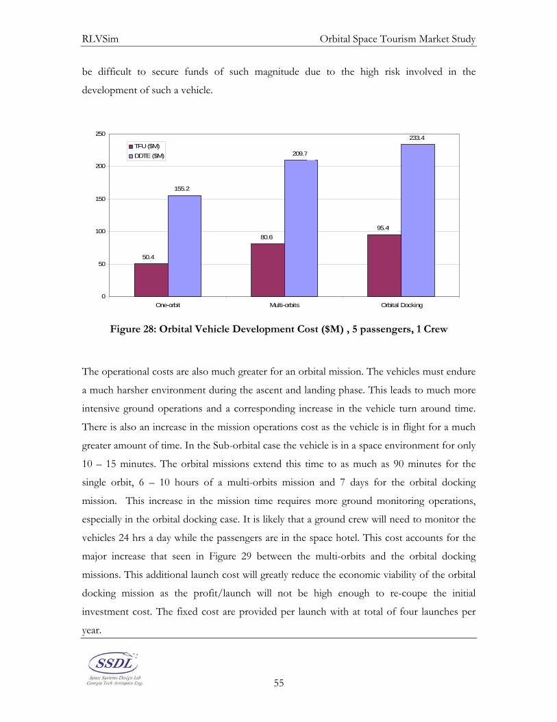
RLVSim Orbital Space Tourism Market Study
be difficult to secure funds of such magnitude due to the high risk involved in the
development of such a vehicle.
50.429
80.6995.49
155.224
209.70
233.42
0
50
100
150
200
250
One-orbit Multi-orbits Orbital Docking
TFU ($M)DDTE ($M)
Figure 28: Orbital Vehicle Development Cost ($M) , 5 passengers, 1 Crew
The operational costs are also much greater for an orbital mission. The vehicles must endure
a much harsher environment during the ascent and landing phase. This leads to much more
intensive ground operations and a corresponding increase in the vehicle turn around time.
There is also an increase in the mission operations cost as the vehicle is in flight for a much
greater amount of time. In the Sub-orbital case the vehicle is in a space environment for only
10 – 15 minutes. The orbital missions extend this time to as much as 90 minutes for the
single orbit, 6 – 10 hours of a multi-orbits mission and 7 days for the orbital docking
mission. This increase in the mission time requires more ground monitoring operations,
especially in the orbital docking case. It is likely that a ground crew will need to monitor the
vehicles 24 hrs a day while the passengers are in the space hotel. This cost accounts for the
major increase that seen in Figure 29 between the multi-orbits and the orbital docking
missions. This additional launch cost will greatly reduce the economic viability of the orbital
docking mission as the profit/launch will not be high enough to re-coupe the initial
investment cost. The fixed cost are provided per launch with at total of four launches per
year.
55
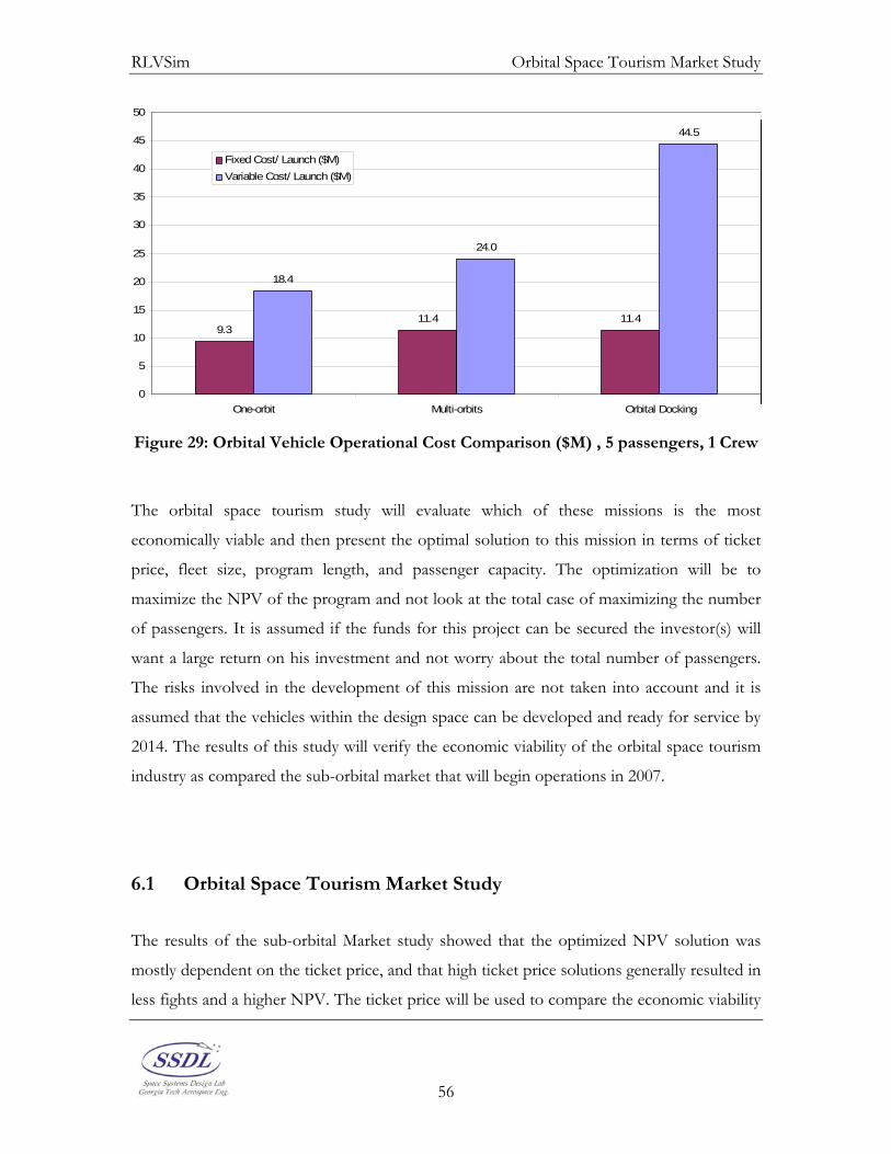
RLVSim Orbital Space Tourism Market Study
9.311.4 11.4
18.4
24.0
44.5
0
5
10
15
20
25
30
35
40
45
50
One-orbit Multi-orbits Orbital Docking
Fixed Cost/ Launch ($M)Variable Cost/ Launch ($M)
Figure 29: Orbital Vehicle Operational Cost Comparison ($M) , 5 passengers, 1 Crew
The orbital space tourism study will evaluate which of these missions is the most
economically viable and then present the optimal solution to this mission in terms of ticket
price, fleet size, program length, and passenger capacity. The optimization will be to
maximize the NPV of the program and not look at the total case of maximizing the number
of passengers. It is assumed if the funds for this project can be secured the investor(s) will
want a large return on his investment and not worry about the total number of passengers.
The risks involved in the development of this mission are not taken into account and it is
assumed that the vehicles within the design space can be developed and ready for service by
2014. The results of this study will verify the economic viability of the orbital space tourism
industry as compared the sub-orbital market that will begin operations in 2007.
6.1 Orbital Space Tourism Market Study
The results of the sub-orbital Market study showed that the optimized NPV solution was
mostly dependent on the ticket price, and that high ticket price solutions generally resulted in
less fights and a higher NPV. The ticket price will be used to compare the economic viability
56

RLVSim Orbital Space Tourism Market Study
of the three missions here as well. The results of this trade study, for a ticket price between
$1 – $15 M, are shown in Figure 30 and a 100% reliability. These three curves exhibit the
same trend with economic viability unobtainable at the low ticket prices. The curve slowly
increase to a peak around a $12 M ticket price for all three missions.
($700.00)
($600.00)
($500.00)
($400.00)
($300.00)
($200.00)
($100.00)
$0.00
$100.00
$200.00
$300.00
0 2 4 6 8 10 12 14 16
Ticket Price ($M)
Net P
rese
nt V
alue
($M
)
Orbital DockingOne -orbitMulti-orbits
Figure 30: Orbital Missions Ticket Price Trade Study.
The unexpected result of this study is that the orbital docking mission is only viable for a
small region of ticket price, while the other two missions have a much wider viable design
space. The NPV for this region is so small as to basically eliminate it from consideration.
This can be explained by the fact that the recurring cost for this mission is so much higher
than the other two. The required monitoring increases the cost such that profit for each
flight can not make back the initial investment cost. Even if this mission showed a positive
NPV it doesn’t provide that much of an increase in demand to justify the increased initial
development and risk involved with developing a vehicle capable of docking with an orbiting
space hotel.
57

RLVSim Orbital Space Tourism Market Study
The other two curves are very similar and show much more promising possibilities. The
single orbit mission actually looks to be the best because its initial investment and operating
cost are much less, and the additional passengers that the multi-orbits mission gets aren’t
enough to offset the difference. However, the single orbit mission is unlikely to be very
enjoyable for most space tourism passengers as it can take a while to adjust to a zero gravity
environment. Therefore it is suggested that the multi-orbit missions provides the most viable
economic solution to the orbital space tourism problem. This mission will be examined
further in the following section.
6.2 Orbital Space Tourism Program Optimization
The optimization of the ticket price was shown in Figure 31 and was determined to be
around $12 M/Launch. This is the same results as seen in the sub-orbital study. There is a
peak in the ticket price for a maximum NPV that occurs at the ticket price were the loss in
passengers becomes too great to be overcome by the marginal increase in revenue. This
limits the number of passengers/year to 32 for a 50% market capture.
The passenger capacity also factors largely into the design of the vehicle as higher passenger
requirements increase the cost and complexity of the vehicle design. The vehicle’s reliability
will be brought back into the problem at this point because the passenger capacity is highly
dependent on the chance of failure. The results for a 100% and 0.995 reliability are shown in
Figure 31, the program length is set to 10 years, the ticket price is set to $12 M, and the fleet
size is set to 1. The 100% case has a peak NPV for a passenger capacity between 4 – 6
passengers. This is the minimum passenger capacity that can meet the passenger demand
without increasing the fleet size above a single vehicle. An additional vehicle would only
decrease the NPV, and would not provide any additional capability. When the reliability is
added to the mission the passenger capacity shifts to a much higher capacity of passengers as
it wants to limit the number of flights. This can bee seen in Figure 31 as the results that
include reliability tend to approach the 100% reliable results as the passenger capacity
increases resulting in a decrease in the number of flights . It is better to spend more money
58

RLVSim Orbital Space Tourism Market Study
up front and design a larger vehicle than it is to risk a failure occurring at some point in the
program. These two curves provide an upper and lower bound on the vehicle passenger
capacity. The more reliable the vehicle is the lower the passenger capacity can be.
($400.00)
($300.00)
($200.00)
($100.00)
$0.00
$100.00
$200.00
$300.00
0 2 4 6 8 10 12 14 16
Passenger Capacity
Net
Pre
sent
Val
ue ($
M)
Reliability = 1.0Reliability = 0.995
Figure 31: Orbital Missions Passenger Capacity Trade Study.
The program length is also an important variable in the design of the overall program
because the longer the vehicle operates the more revenue it can generate and the greater the
return on investment. This is true for the case where the vehicle doesn’t experience a chance
of failure, however in the case where there is a chance of vehicle failure there is maximum
number of years the vehicles can operate before the chance of failure increase such that a
failure occurs in almost every simulation and a greater NPV can not be achieved. Therefore
there is a balance between the number of years that the vehicle brings in revenue and the
chance of failure that occurs for an increase in the number of flights. In this case this
optimal program length is 10 years, after that the chance of a failure occurring is too high for
the program to be economically viable. These results can be seen in Figure 32.
59

RLVSim Orbital Space Tourism Market Study
$0.00
$50.00
$100.00
$150.00
$200.00
$250.00
$300.00
0 5 10 15 20 25
Operating Years
Net
Pre
sent
Val
ure
($M
)
Reliability = 1.0
Reliability = 0.995
Figure 32: Orbital Missions Operating Trade Study.
The final variable of interest was the vehicle fleet size. The passenger demand for a orbital-
space program is not very large, the profit is made from price not volume, and so a large
fleet size is not required. The results run above were all for a single vehicle because that is all
that is required to meet the demand, assuming a 30-day turn around time. Increasing the
number of vehicles only decreases the NPV because the additional vehicles don’t add any
additional capability. Even in the case with reliability the NPV is maximized for single
vehicle. In reality additional vehicles may be needed to account for unexpected problems
that may cause a delay in a vehicle launch. Additional vehicles will help to guarantee that the
launch schedule remains intact.
The optimized program for an orbital space tourism mission is given by the following
• Mission: Multi-orbits
• Ticket Price: $12 M
• Passenger Capacity: Depends on reliability (6-10 passengers)
• Program Length: 10 years
• Fleet Size: 1 vehicle
60

RLVSim Conclusion – Viability of Future Space Tourism Market
7.0 Conclusion – Viability of Future Space Tourism Market
The space tourism study presented here utilized an updated version of the economic analysis
tool LMNoP to conduct a series of studies to determine the economic viability of the space
tourism market. The updated version of LMNoP included an update of the passenger
demand market model derived from the market data collected by the Futron Corporation.
This economic analysis determined that the Virgin Galactic model is an economically viable
market in its current form as long as a failure doesn’t occur during the life of the program, if
one does occur the recovery expresses are too great to overcome. It was also determined
that the Virgin Galactic model is likely operating under the idea that the goal of space
tourism industry is to provide as many flights as possible and making a profit is secondary.
The Virgin Galactic model showed very similar results to the sub-orbital program optimized
for maximum total number of passengers, where the ticket price should be set as low as
possible such that the program can still keep a positive NPV. The study also found that the
optimal program to maximize the economic viability of a space tourism company is to set
the ticket price slightly less then $1 M, have a high passenger capacity (10 Passengers/flight)
and to operate only a single vehicle. This will provide the largest NPV, but at the same time
many less passengers will be able to afford a ride. The orbital space tourism market is most
likely to succeed when a multi-orbits mission is employed. The program again wants to
charge a very high ticket price, $12 M and operate only a single vehicle for 10 year period.
The passenger capacity is highly dependent on the reliability of the vehicle and should be
kept in the range of 6 – 10 passengers/Vehicle.
The results of this study have concluded that the space tourism industry is a very viable
economic market and has great possibilities for the future. With the successful launch of
SpaceShipOne and the formation of Virgin Galactic, the next generation in space adventure
has begun.
61

RLVSim Appendix A: Monet Carlo Triangular Distributions
Appendix A: Monet Carlo Triangular Distributions
0.85 0.925 1 1.075 1.15 Baseline Passenger Demand
0.9 1.05 1.2 1.35 1.5 Development Cost
0.9 1.05 1.2 1.35 1.5 Production Cost
0.9 1.05 1.2 1.35 1.5 Operating Cost
62

RLVSim Appendix B: Tourism Vehicle Model Orbital Example
Appendix B: Tourism Vehicle Model Orbital Example
First Stage –
Level 2 Level 1Wing Group 11,298Tail Group 5,491Body Group 48,737
Primary Structure 34,686.113Seondary Sructure 1,020.180Crew Cabin 0.000Body Flap 0.000Thrust Structure 2,068.562LOX Tank 4,197.435LH2 Tank 6,765.152
Thermal Protection 0Landing Gear 10,676Main Propulsion 18,604RCS Propulsion 0OMS Propulsion 0Primary Power 991Electrical Conversion & Dist. 7,710Hydraulic System 0System Control Actuation 1,558Avionics 1,750Envronmental Control 1,326Personal Equipment 0Dry Weight Margin 16,221
Dry Weight 124,362
Crew and Gear 0Payload Provisions 0Cargo (Delivered & Returned) 192,851Residual Propellants 4,024
Main Propellant Residuals 2,889LOXLH2
RCS/OMS Residuals 1,135OMS/RCS Reserve Propellants 2,270
Landed Weight 323,508
RCS Entry Propellants 1,091
Entry Weight 324,599
RCS/OMS Propellants (on-orbit) 21,613OMS 18,960RCS 2,653
Cargo Discharge 0Ascent Reserve Propellants 2,889
LOX 2,524LH2 366
Inflight Losses and Vents 3,246
Insertion Weight 352,347
Ascent Propellants 577,849LOX 504,704LH2 73,145
Gross Liftoff Weight 930,197
Startup Losses 5,778LOX 5,047LH2 731
Maximum Pre-Launch Weight 935,975
63

RLVSim Appendix B: Tourism Vehicle Model Orbital Example
Second Stage
Level 2 Level 11.0 Wing Group 1,5882.0 Tail Group 9503.0 Body Group 14,146
Primary Structure 8,776Seondary Sructure 413Crew Cabin 2,272Body Flap 0Thrust Structure 426LOX Tank 865LH2 Tank 1,394
4.0 Thermal Protection 6,4725.0 Landing Gear 2,2006.0 Main Propulsion 3,8337.0 RCS Propulsion 7498.0 OMS Propulsion 7819.0 Primary Power 6,14410.0 Electrical Conversion & Dist. 3,54011.0 Hydraulic System 012.0 System Control Actuation 32113.0 Avionics 1,75014.0 Envronmental Control 4,16615.0 Personal Equipment 3,01516.0 Dry Weight Margin 7,448
Dry Weight 57,104
17.0 Crew and Gear 8,25618.0 Payload Provisions 019.0 Cargo (Delivered & Returned) 020.0 Residual Propellants 829
Main Propellant Residuals 595LOXLH2
RCS/OMS Residuals 23421.0 OMS/RCS Reserve Propellants 468
Landed Weight 66,657
22.0 RCS Entry Propellants 225
Entry Weight 66,881
23.0 RCS/OMS Propellants (on-orbit) 4,453OMS 3,907RCS 547
24.0 Cargo Discharge 025.0 Ascent Reserve Propellants 595
LOX 520LH2 75
26.0 Inflight Losses and Vents 669
Insertion Weight 72,599
27.0 Ascent Propellants 119,062LOX 103,991LH2 15,071
Gross Liftoff Weight 191,661
28.0 Startup Losses 1,191LOX 1,040LH2 151
Maximum Pre-Launch Weight 192,851
64

RLVSim Appendix C: Vehicle Gross/Dry Weight Curve Fits
Appendix C: Vehicle Gross/Dry Weight Curve Fits
Sub-orbital
8.41289.8279.
2.60115.230971.12
1
21
++−=
++−=
xxDWxxGW
2.35661.239546.29.41697.385978.2
22
22
++−=
++−=
xxDWxxGW
One-Orbit
95226.42122.4
416091.240864.202
1
21
++−=
++−=
xxDWxxGW
8.41456.27558.2
88838.7172.52
2
22
++−=
++−=
xxDWxxGW
Multi-orbits
7.159011.70405.7
6948753.402146.342
1
21
++−=
++−=
xxDWxxGW
5.692325.46031.46.148347.119868.8
22
22
++−=
++−=
xxDWxxGW
Orbital Docking
190442.843441.8
832182.481627.412
1
21
++−=
++−=
xxDWxxGW
6.82912.551162.5
177666.143539.102
2
22
++−=
++−=
xxDWxxGW
65

RLVSim References
References
[1] Olds, J, McCormick, D, Charania, A, Marcus, L, “Space Tourism: Making it
Work for Fun and Profit,” IAf paperIAA-00-IAA.1.3.05, October 2000. [2] Beard, A., Starzyk, J., “Space Tourism Market Study”, Futron Corporation,
Bethesda, MD, October 2002. [3] Commercial Space Transportation Study Final Report, Boeing, General Dynamics,
Lockheed, Martin Marietta, McDonnell Douglas and Rockwell, pp. 198-229, April 1994.
[4] Nagatomo, M. and Collins, P., “A Common Cost Target of Space Transportation for
Space Tourism and Space Energy Development,” AAS 97-460, pp. 617-630. [5] Reifert, Jane, President of Incredible Adventures, Personal Correspondence, Jan
2005. [6] Goehlich, R.A.: Space Tourism: Economic and technical Evaluation of Suborbital
Space Flights for Tourism, ISBN 3-936231-36-2, Der Andere Verlag, Osnabruck, Germany, 2002
[7] Isakowitz, S., International Reference Guide to Space Launch Systems, Reston,
VA, 2004. [8] “Spacecraft/Vehicle Level Cost Model,” Johnson Spaceflight Center, Texas,
February 2005, [http://www1.jsc.nasa.gov/bu2/SVLCM.html accessed 2/2005.] [9] Koelle, D., Handbook of Cost Engineering: For Space Transportation Systems
with TRANSCOST 7.0, Liebigweg, Germany, 2000. [10] “Virgin Galactic”,2005, [http://www.virgingalactic.com/ accessed 4/2005.]
66