probabilistic analysis of circular tunnels in...

Probabilistic Analysis of Circular Tunnels in HomogeneousSoil Using Response Surface Methodology

Guilhem Mollon1; Daniel Dias2; and Abdul-Hamid Soubra, M.ASCE3

Abstract: A probabilistic analysis of a shallow circular tunnel driven by a pressurized shield in a frictional and/or cohesive soil ispresented. Both the ultimate limit state �ULS� and serviceability limit state �SLS� are considered in the analysis. Two deterministic modelsbased on numerical simulations are used. The first one computes the tunnel collapse pressure and the second one calculates the maximalsettlement due to the applied face pressure. The response surface methodology is utilized for the assessment of the Hasofer-Lind reliabilityindex for both limit states. Only the soil shear strength parameters are considered as random variables while studying the ULS. However,for the SLS, both the shear strength parameters and Young’s modulus of the soil are considered as random variables. For ULS, theassumption of uncorrelated variables was found conservative in comparison to the one of negatively correlated parameters. For both ULSand SLS, the assumption of nonnormal distribution for the random variables has almost no effect on the reliability index for the practicalrange of values of the applied pressure. Finally, it was found that the system reliability depends on both limit states. Notice however thatthe contribution of ULS to the system reliability was not significant. Thus, SLS can be used alone for the assessment of the tunnelreliability.

DOI: 10.1061/�ASCE�GT.1943-5606.0000060

CE Database subject headings: Shields, tunneling; Settlement; Serviceability; Ultimate loads; Limit states; System reliability.

Introduction

The stability analysis of tunnels and the computation of soil dis-placements due to tunneling were commonly performed usingdeterministic approaches �e.g., Jardine et al. 1986; Dias et al.1997; Potts and Addenbrooke 1997; Dias et al. 2002; Yoo 2002;Jenck and Dias 2003; Mroueh and Shahrour 2003; Ribeiro eSousa et al. 2003; Jenck and Dias 2004; Dias and Kastner 2005;Wong et al. 2006; Eclaircy-Caudron et al. 2007�. A reliability-based approach for the analysis of tunnels is more rational since itenables one to consider the inherent uncertainty of the input pa-rameters. In this paper, a reliability-based analysis of a shallowcircular tunnel driven by a pressurized shield in a c−� soil ispresented. Both the ultimate limit state �ULS� and the serviceabil-ity limit state �SLS� are considered in the analysis. Two determin-istic models based on the Lagrangian explicit finite-differencecode FLAC3D �1993� are used. The first one involves the tunnelface stability in the ULS and focuses on the computation of thetunnel collapse pressure. The second one emphasizes the SLS and

1Ph.D. Student, INSA Lyon, LGCIE Site Coulomb 3, Géotechnique,Bât. J.C.A. Coulomb, Domaine Scientifique de la Doua, 69621 Villeur-banne Cedex, France. E-mail: [email protected]

2Associate Professor, INSA Lyon, LGCIE Site Coulomb 3, Géotech-nique, Bât. J.C.A. Coulomb, Domaine Scientifique de la Doua, 69621Villeurbanne Cedex, France. E-mail: [email protected]

3Professor, Institut de Recherche en Génie Civil et Mécanique, Univ.of Nantes, UMR CNRS 6183, Bd. de l’université, BP 152, 44603 Saint-Nazaire, France �corresponding author�. E-mail: [email protected]

Note. This manuscript was submitted on July 30, 2008; approved onJanuary 13, 2009; published online on February 23, 2009. Discussionperiod open until February 1, 2010; separate discussions must be submit-ted for individual papers. This paper is part of the Journal of Geotech-nical and Geoenvironmental Engineering, Vol. 135, No. 9, September 1,
2009. ©ASCE, ISSN 1090-0241/2009/9-1314–1325/$25.00.
1314 / JOURNAL OF GEOTECHNICAL AND GEOENVIRONMENTAL ENGIN

Downloaded 15 Aug 2009 to 213.255.225.31. Redistribution subject to

calculates the maximal settlement due to the applied face pres-sure. The response surface methodology �RSM� is utilized to findan approximation of the analytically unknown performance func-tion and the corresponding reliability index for both limit states.The random variables considered in the analysis are the soil shearstrength parameters c and � for the ULS. However, for the SLS,both the shear strength parameters and Young’s modulus of thesoil are used. After a brief description of the two deterministicmodels, the basic concepts of the theory of reliability are pre-sented. Then, the probabilistic analysis and the corresponding nu-merical results are presented and discussed.

Deterministic Numerical Modeling of Tunnel FaceStability and Face Pressure-Induced DisplacementUsing FLAC3D

FLAC3D is a commercially available three-dimensional finite-difference code, in which an explicit Lagrangian calculationscheme and a mixed discretization zoning technique are used.This code includes an internal programing option �FISH�, whichenables the user to add his own subroutines. In this software,although a static �i.e., nondynamic� mechanical analysis is re-quired, the equations of motion are used. The solution to a staticproblem is obtained through the damping of a dynamic process byincluding damping terms that gradually remove the kinetic energyfrom the system. A key parameter used in the software is theso-called “unbalanced force ratio.” It is defined at each calcula-tion step �or cycle� as the average unbalanced mechanical forcefor all the grid points in the system divided by the average appliedmechanical force for all these grid points. The system may bestable �called also in a steady state of static equilibrium� or un-stable �called also in a steady state of plastic flow�. A steady stateof static equilibrium is one for which a state of static equilibrium
is achieved in the soil-structure system due to given service loads
EERING © ASCE / SEPTEMBER 2009

ASCE license or copyright; see http://pubs.asce.org/copyright

and for which the unbalanced force ratio decreases with the num-ber of cycles increase and then it becomes less than a prescribedtolerance �e.g., 10−5 as suggested in FLAC3D software�. On theother hand, a steady state of plastic flow is one in which soilfailure is achieved. In this case, the unbalanced force ratio de-creases with the number of cycles increase and then attains aquasi-constant nonvarying value. This value is higher than the onecorresponding to the steady state of static equilibrium.

Numerical Simulations

This section focuses on �1� the face stability analysis at ULS and�2� the assessment of face pressure-induced soil displacements atSLS, in the case of a circular tunnel driven by a pressurizedshield. A uniform retaining pressure is applied to the tunnel faceto simulate tunneling under compressed air. Although a randomsoil is studied in this paper, the deterministic FLAC3D simulationsconsider a homogeneous soil. The randomness of the soil is takeninto account from one simulation to another. Because of symme-try, only one-half of the entire domain is considered in the analy-sis, as shown in Fig. 1 �the velocity field being symmetrical withrespect to the vertical plane passing through the longitudinal axisof the tunnel�. A nonsymmetrical velocity field would be neces-sary only for the computation of the reliability of a tunnel in aspatially variable soil �i.e., where the random parameters are con-sidered as random processes�. In all subsequent calculations ofthe ULS and SLS, the following procedure is performed beforeany simulation: geostatic stresses are first applied to the soil, thenseveral cycles are run in order to arrive at a steady state of staticequilibrium, and finally, the obtained displacements are set to zeroin order to obtain the soil displacements due only to the pressureapplied on the tunnel face.

ULS: Face Stability Analysis

Although the present section is intended to the evaluation of thetunnel face stability, no safety factor is calculated. Indeed, onlythe highest pressure applied to the tunnel face for which soilcollapse would occur is computed. This collapse pressure is theone for which the soil in front of the tunnel face undergoes down-ward movement. It is called the tunnel active pressure.

A circular tunnel of diameter D=10 m and cover C=10 m

Fig. 1. Soil domain and mesh used in FLAC3D for ULS

�i.e., C /D=1� driven in a c−� soil is considered in this paper �cf.

JOURNAL OF GEOTECHNICAL AND GEOEN


Fig. 1�. The size of the numerical model is 50 m in the X direc-tion, 26 m in the Z direction, and 40 m in the Y direction. Thesedimensions are chosen so as not to affect the value of the tunnelcollapse pressure. A three-dimensional nonuniform mesh is used.The present model is composed of approximately 27,000 zones.The tunnel face region was subdivided into 198 zones since veryhigh stress gradients were developed in that region.

For the displacement boundary conditions, the bottom bound-ary was assumed to be fixed and the vertical boundaries wereconstrained in motion in the normal direction.

A conventional elastic perfectly plastic model based on theMohr-Coulomb failure criterion was adopted to represent the soil.The soil elastic properties employed are Young’s modulus E=240 MPa and Poisson’s ratio �=0.3. The values of the angle ofinternal friction and cohesion of the soil used in the analysis are�=17° and c=7 kPa, respectively. The soil dilation angle � wasassumed equal to zero in accordance with the commonly usedrelationship �=�−30°. The soil unit weight was taken equal to18 kN /m3. Notice that the soil elastic properties have a negli-gible effect on the collapse pressure. A concrete lining of 0.4-mthickness is used in the analysis. The lining is simulated by a shellof linear elastic behavior. Its elastic properties are Young’s modu-lus E=15 GPa and Poisson’s ratio �=0.2. The lining is connectedto the soil via interface elements that follow Coulomb’s law. Theinterface is assumed to have a friction angle equal to two-thirds ofthe soil angle of internal friction �i.e., 11,3°� and cohesion equalto zero. Normal stiffness Kn=1011 Pa /m and shear stiffness Kn

=1011 Pa /m were assigned to this interface. These parameters area function of the neighboring elements rigidity �FLAC3D 1993�and do not have a major influence on the collapse pressure.

For the computation of a tunnel collapse pressure usingFLAC3D, a stress control method is adopted in this paper. Noticethat a displacement control method could be used instead since itrequires much less computation time. However, this approach re-quires a priori assumption concerning the distribution of the dis-placement on the tunnel face �e.g., uniform or parabolicdistribution, etc.� and may lead to erroneous results. The nextsection is devoted to the presentation of the stress control methodused for the computation of the tunnel collapse pressure.

Stress Control MethodTwo methods may be used for the computation of the tunnelcollapse pressure. The first one is the simple bisection approachand the second one is called the improved bisection method. Inthe simple bisection approach, simulations are run for a series oftrial values of the tunnel pressure �trial. The value of �trial at whichfailure occurs is found using bracketing and bisection approachesas follows:1. Upper and lower brackets are first established.• The initial lower bracket corresponds to any trial pressure for

which the system is unstable. This state corresponds to a non-null face extrusion velocity at each point of the tunnel face�see, for instance, the horizontal velocity of Point A shown inFig. 2�b� where Point A is located at the centre of the tunnelface�. This nonnull velocity at Point A corresponds to a con-tinuously increasing horizontal displacement at this point, asshown in Fig. 2�a�, and it means that a steady state of failure orplastic flow is achieved in this case.

• The initial upper bracket corresponds to any trial pressure inwhich the system is stable. This state corresponds to a zeroface extrusion velocity at each point of the tunnel face �see, forinstance, the horizontal velocity of Point A shown in Fig.
2�b��. This zero velocity at Point A corresponds to a constant
VIRONMENTAL ENGINEERING © ASCE / SEPTEMBER 2009 / 1315


horizontal displacement at this point as long as the number ofcycles increases, as shown in Fig. 2�a�, and it means that asteady state of static equilibrium is achieved in this case.

2. Next, a new value, midway between the upper and lowerbrackets, is tested. If the system is stable for this midwayvalue, the upper bracket is replaced by this new trial pres-sure. If the system does not reach equilibrium, the lowerbracket is then replaced by the midway value.

3. Steps 1 and 2 are repeated until the difference between upperand lower brackets is less than a specific tolerance.

The simple bisection method consists of running severalcycles for the two states of plastic flow and static equilibriumcorresponding, respectively, to the lower and upper brackets. Thisprocedure is very time consuming because the plastic flow stateusually occurs after a large number of cycles. This can be dra-matic if one is looking for a precise value of the collapse pressure.A more efficient method called in this paper as “the improvedbisection approach” may be used. It allows one to check if thesystem is unstable much more quickly than the classical ap-proach. This method is similar to that used in FLAC3D softwarefor the determination of the safety factor. It may be briefly de-scribed as follows. First, a very high value of the cohesion isaffected to the soil. This makes the soil behave as an elasticmaterial. Second, the whole system is set to an unbalanced stateby doubling artificially all the values of the internal stresses. Themethod consists of determining a “representative” number N ofcycles. It corresponds to the number of computation cycles thatthe software must run to return to a static equilibrium state fromthe previous unbalanced state. This number is generally close to3,000 steps. When N is determined, the initial value of the cohe-sion is restored. The system is considered in a steady state ofplastic flow if it remains unstable after performing these N cycles.As one can easily see, there is no need to run a large number ofcycles to check the instability of the system in the improved bi-section method. Interested readers by this method may refer formore details to Fast Lagrangian Analysis of Continua �FLAC3D��1993�. The improved bisection method was coded in FISH lan-guage into the FLAC3D software. It allows one to obtain the col-

Fig. 2. �a� Horizontal displacement; �b� horizontal velocity of Point A�plastic flow�

lapse pressure more quickly than the classical bisection approach.



The CPU time is variable but can be longer than 1 day whenusing the classical bisection method and becomes equal to 90 min�on a Core2 Quad CPU 2.40-GHz PC� when one uses the im-proved bisection method. Thus, the improved bisection techniqueis adopted for the computation of the tunnel collapse pressure.Bracketing and bisection are repeated until the difference betweenthe upper and lower brackets becomes smaller than a prescribedtolerance �e.g., 100 Pa in this paper�. The tunnel face collapsepressure was found equal to �c=34.5 kPa. The correspondingcollapse velocity field given by FLAC3D is provided in Fig. 3.Stability against collapse is ensured as long as the applied pres-sure �t is greater than the tunnel collapse pressure �c.

SLS: Maximal Settlement

First, it should be emphasized here that the deterministic numeri-cal simulations used in the paper for the SLS are limited to thecomputation of the ground settlement due to only the applied facepressure. Notice however that the ground settlement is primarilydue to the shield tail void. In real shield tunneling cases, theproportion of ground settlement induced by the face pressure maybe less than 25% of the total settlement �cf. Vanoudheusden2006�. The settlement due to shield tunneling is pretty much af-fected by the closure of tail void, grouting, unlined length, soil

ter of tunnel face� during stability �static equilibrium� and instability

Fig. 3. Collapse velocity field ��c=34.5 kPa�

�cen



loss, etc., during tunneling. Thus, the present numerical simula-tions can only be regarded as an idealized condition ignoringmany important factors concerning tunneling construction. Thewriters consider the ground settlement due to the sole effect of theface pressure for the following reasons. The face pressure is theparameter that has the most influence on stability. On the otherhand, several parameters �among them the face pressure� wouldinfluence the ground settlement. In this paper, the effect of onlyone tunneling parameter �i.e., the face pressure� on both the sta-bility and deformation analyses of the pressurized shield tunnel-ing was considered in order to be able to make a comparison ofthe tunnel reliability on both the SLS and ULS due to this uniqueparameter.

For the computation of the maximal settlement due to an ap-plied pressure �t on the tunnel face, the excavation by the shieldis also modeled here by the stress control method in order to takeinto account the excavation steps. Contrary to the ULS where theexcavation steps were not necessary in the computation procedureof the collapse pressure, in the present SLS, a total of 50 excava-tion steps �with a length of 1 m for each step� were performed.Cycling was performed after each excavation step in order toobtain the corresponding displacement. It should be mentionedhere that the excavation and the concrete lining installation wereapplied concurrently. This leads, as mentioned before, to a signifi-cant simplification concerning the simulation of tunneling con-struction and provides the settlement induced by only the facedecompression.

An elastic perfectly plastic model is still used here for the soilsince it enables the development of plastic zones that may occurnear the tunnel face for the entire range of variation in the appliedpressure �t and it leads to more accurate solutions than a purelyelastic model. A more sophisticated model including nonlinearityin the elastic range would be of interest and may give betterresults for the settlement. However, it is out of the scope of thispaper and will be used in a future research. The numerical simu-lations have shown that the longitudinal limits of the model havea significant influence on the value of the maximal settlement.This is the reason why the mesh used for the assessment of themaximal settlement is much more extended than the previous onealong the Y axis. Notice however that the same geometry isadopted here in the X-Z section. The mesh used is presented inFig. 4. Fig. 5�a� shows the settlement along the Y axis after 50steps of excavation for an applied pressure of 40 kPa. This curveclearly shows the zone, which is significantly influenced by theboundary Y =0 of the model. The maximal settlement �4.7 mm inthis case� occurs about 10 m behind the tunnel face. Fig. 5�b�

Fig. 4. Soil domain and mesh used in FLAC3D for SLS

presents the maximal settlement versus the number of excavation



steps. This figure shows the stabilization of the maximal settle-ment after about 30 steps of 1 m long. Thus, one can concludethat the 50 steps of excavation adopted in this paper are sufficientto give accurate result for the maximal settlement. Finally, noticethat the CPU time required for each computation of the maximalsettlement was found to be 130 min on a Core2 Quad CPU 2.40-GHz PC.

Ellipsoid Approach in Reliability Theory

The reliability index of a geotechnical structure is a measure ofthe safety that takes into account the inherent uncertainties of theinput parameters. A widely used reliability index is the Hasoferand Lind �1974� index. Its matrix formulation is �Ditlevsen 1981�

�HL = minx�F

��x − �x�TC−1�x − �x� �1�

in which x=vector representing the n random variables; �x

=vector of their mean values; and C=their covariance matrix.The minimization of Eq. �1� is performed subject to the constraintG�x��0, where the limit state surface G�x�=0 separates then-dimensional domain of random variables into two regions: afailure region F represented by G�x��0 and a safe region givenby G�x��0.

Low and Tang �1997a, 2004� introduced the concept of anexpanding ellipsoid �or ellipse in the two-dimensional case�, asshown in Fig. 6, and led to a simple method of computing theHasofer-Lind reliability index in the physical space of the randomvariables. These writers reported that the Hasofer-Lind reliabilityindex �HL may be regarded as the codirectional axis ratio of the

Fig. 5. Settlement determination in SLS: �a� settlement along Y axisafter 50 excavation steps when �t=40 kPa; �b� maximal settlementversus number of excavation steps

smallest ellipsoid that just touches the limit state surface to the



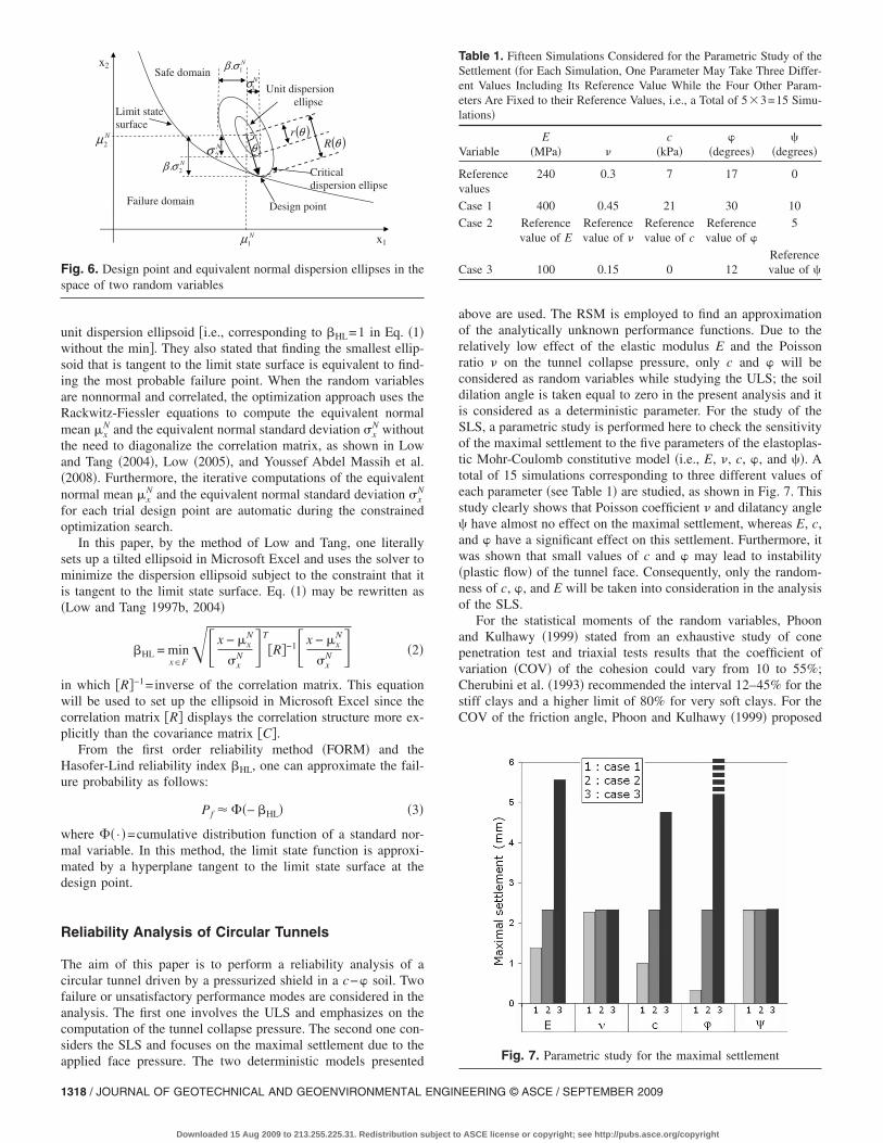
unit dispersion ellipsoid �i.e., corresponding to �HL=1 in Eq. �1�without the min�. They also stated that finding the smallest ellip-soid that is tangent to the limit state surface is equivalent to find-ing the most probable failure point. When the random variablesare nonnormal and correlated, the optimization approach uses theRackwitz-Fiessler equations to compute the equivalent normalmean �x

N and the equivalent normal standard deviation �xN without

the need to diagonalize the correlation matrix, as shown in Lowand Tang �2004�, Low �2005�, and Youssef Abdel Massih et al.�2008�. Furthermore, the iterative computations of the equivalentnormal mean �x

N and the equivalent normal standard deviation �xN

for each trial design point are automatic during the constrainedoptimization search.

In this paper, by the method of Low and Tang, one literallysets up a tilted ellipsoid in Microsoft Excel and uses the solver tominimize the dispersion ellipsoid subject to the constraint that itis tangent to the limit state surface. Eq. �1� may be rewritten as�Low and Tang 1997b, 2004�

�HL = minx�F�� x − �x

N

�xN �T

�R�−1� x − �xN

�xN � �2�

in which �R�−1=inverse of the correlation matrix. This equationwill be used to set up the ellipsoid in Microsoft Excel since thecorrelation matrix �R� displays the correlation structure more ex-plicitly than the covariance matrix �C�.

From the first order reliability method �FORM� and theHasofer-Lind reliability index �HL, one can approximate the fail-ure probability as follows:

Pf � �− �HL� �3�

where � · �=cumulative distribution function of a standard nor-mal variable. In this method, the limit state function is approxi-mated by a hyperplane tangent to the limit state surface at thedesign point.

Reliability Analysis of Circular Tunnels

The aim of this paper is to perform a reliability analysis of acircular tunnel driven by a pressurized shield in a c−� soil. Twofailure or unsatisfactory performance modes are considered in theanalysis. The first one involves the ULS and emphasizes on thecomputation of the tunnel collapse pressure. The second one con-siders the SLS and focuses on the maximal settlement due to the

Failure domain

Safe domain

Limit state

surface

Design point

Critical

dispersion ellipse

N

2.σβ

N

2σ

N

1σUnit dispersion

ellipse

N

1µ

N

2µ

x1

x2 N

1.σβ

( )θr

( )θRθ

Fig. 6. Design point and equivalent normal dispersion ellipses in thespace of two random variables

applied face pressure. The two deterministic models presented



above are used. The RSM is employed to find an approximationof the analytically unknown performance functions. Due to therelatively low effect of the elastic modulus E and the Poissonratio � on the tunnel collapse pressure, only c and � will beconsidered as random variables while studying the ULS; the soildilation angle is taken equal to zero in the present analysis and itis considered as a deterministic parameter. For the study of theSLS, a parametric study is performed here to check the sensitivityof the maximal settlement to the five parameters of the elastoplas-tic Mohr-Coulomb constitutive model �i.e., E, �, c, �, and ��. Atotal of 15 simulations corresponding to three different values ofeach parameter �see Table 1� are studied, as shown in Fig. 7. Thisstudy clearly shows that Poisson coefficient � and dilatancy angle� have almost no effect on the maximal settlement, whereas E, c,and � have a significant effect on this settlement. Furthermore, itwas shown that small values of c and � may lead to instability�plastic flow� of the tunnel face. Consequently, only the random-ness of c, �, and E will be taken into consideration in the analysisof the SLS.

For the statistical moments of the random variables, Phoonand Kulhawy �1999� stated from an exhaustive study of conepenetration test and triaxial tests results that the coefficient ofvariation �COV� of the cohesion could vary from 10 to 55%;Cherubini et al. �1993� recommended the interval 12–45% for thestiff clays and a higher limit of 80% for very soft clays. For theCOV of the friction angle, Phoon and Kulhawy �1999� proposed

Table 1. Fifteen Simulations Considered for the Parametric Study of theSettlement �for Each Simulation, One Parameter May Take Three Differ-ent Values Including Its Reference Value While the Four Other Param-eters Are Fixed to their Reference Values, i.e., a Total of 53=15 Simu-lations�

VariableE

�MPa� �c

�kPa��

�degrees��

�degrees�

Referencevalues

240 0.3 7 17 0

Case 1 400 0.45 21 30 10

Case 2 Referencevalue of E

Referencevalue of �

Referencevalue of c

Referencevalue of �

5

Case 3 100 0.15 0 12Referencevalue of �

Fig. 7. Parametric study for the maximal settlement



the interval of 5–15%. For the COV of Young’s modulus, thesame authors proposed 30%, Bauer and Pula �2000� suggested15%, and Baecher and Christian �2003� proposed the interval2–42%. The illustrative values used in this paper for the statisticalmoments of the shear strength parameters and Young’s modulusbelong to the intervals proposed by the above cited authors andare given as follows: �c=7 kPa, ��=17°, �E=240 MPa,COVc=20%, COV�=10%, and COVE=15%. For the probabilitydistribution of the random variables, two cases may be studied. Inthe first case, referred to as normal variables, c, �, and E areconsidered as normal variables. In the second case, referred to asnonnormal variables, c and E are assumed to be lognormally dis-tributed while � is assumed to be bounded and a beta distributionis used �Fenton and Griffiths 2003�. The parameters of the betadistribution are determined from the mean value and standarddeviation of � �Haldar and Mahadevan 2000�. It should be men-tioned that for the ULS for which only the shear strength param-eters are considered as random variables, E will be considered asdeterministic with its mean value and with a zero COV. Concern-ing the coefficients of correlation between random variables, onlya negative correlation between c and � with ��c,�=−0.5� is as-sumed to exist when these random variables are considered ascorrelated.

After a brief description of the performance functions used inthe present analysis, the RSM and its numerical implementationare presented. Then, the probabilistic numerical results based onthis method are presented and discussed.

Performance Functions

Two performance functions are used in the reliability analysis.The first one is defined with respect to the collapse mode offailure in the ULS as follows:

G1 =�t

�c− 1 �4�

where �t=applied pressure on the tunnel face and �c=tunnel col-lapse pressure computed using FLAC3D. The second performancefunction, which is defined in the SLS with respect to a prescribedadmissible settlement, is given as follows:

G2 = �max − � �5�

where �=maximal settlement �as explained before� calculated byFLAC3D due to an applied pressure �t and �max=maximal admis-sible prescribed settlement.

Response Surface Method

When using numerical simulations, the closed form solution ofthe performance function is not available. Thus, the determinationof the reliability index is not straightforward. An algorithm basedon the RSM proposed by Tandjiria et al. �2000� is used in thispaper with the aim to calculate the reliability index and the cor-responding design point. The basic idea of this method is to ap-proximate the performance function by an explicit function of therandom variables and to improve the approximation via iterations.The approximate performance function widely used in literaturehas a quadratic form. It uses a second order polynomial with
squared terms. The expression of this approximation is given by


G�x� = a0 + i=1

n

aixi + i=1

n

bixi2 �6�

where xi=random variables; n=number of the random variables;and �ai ,bi�=coefficients to be determined. In this paper, two ran-dom variables c and � are considered for the ULS �i.e., n=2�.However, n=3 for the SLS since the random variables used inthat case are c, �, and E. For both limit states, the random vari-ables are characterized by their mean values �i and their COVs�i. A brief explanation of the algorithm used is as follows:1. Evaluate the performance function G�x� at the mean value

point � and the 2n points each at ��k�, where k is usuallyequal to 1 �this parameter may be varied in some cases ifnecessary�.

2. The above 2n+1 values of G�x� can be used to solve Eq. �6�for the coefficients �ai ,bi�. This obtains a tentative responsesurface function.

3. Solve Eq. �1� to obtain a tentative design point and a tenta-tive �HL subject to the constraint that the tentative responsesurface function of Step 2 be equal to zero.

4. Repeat Steps 1–3 until convergence. Each time Step 1 isrepeated, the 2n+1 sampled points are centered at the newtentative design point of Step 3.

Notice finally that Steps 2 and 3 were done using the optimizationtools in Microsoft Excel. However, Step 1 was performed usingdeterministic FLAC3D calculations.

Numerical Results

ULS

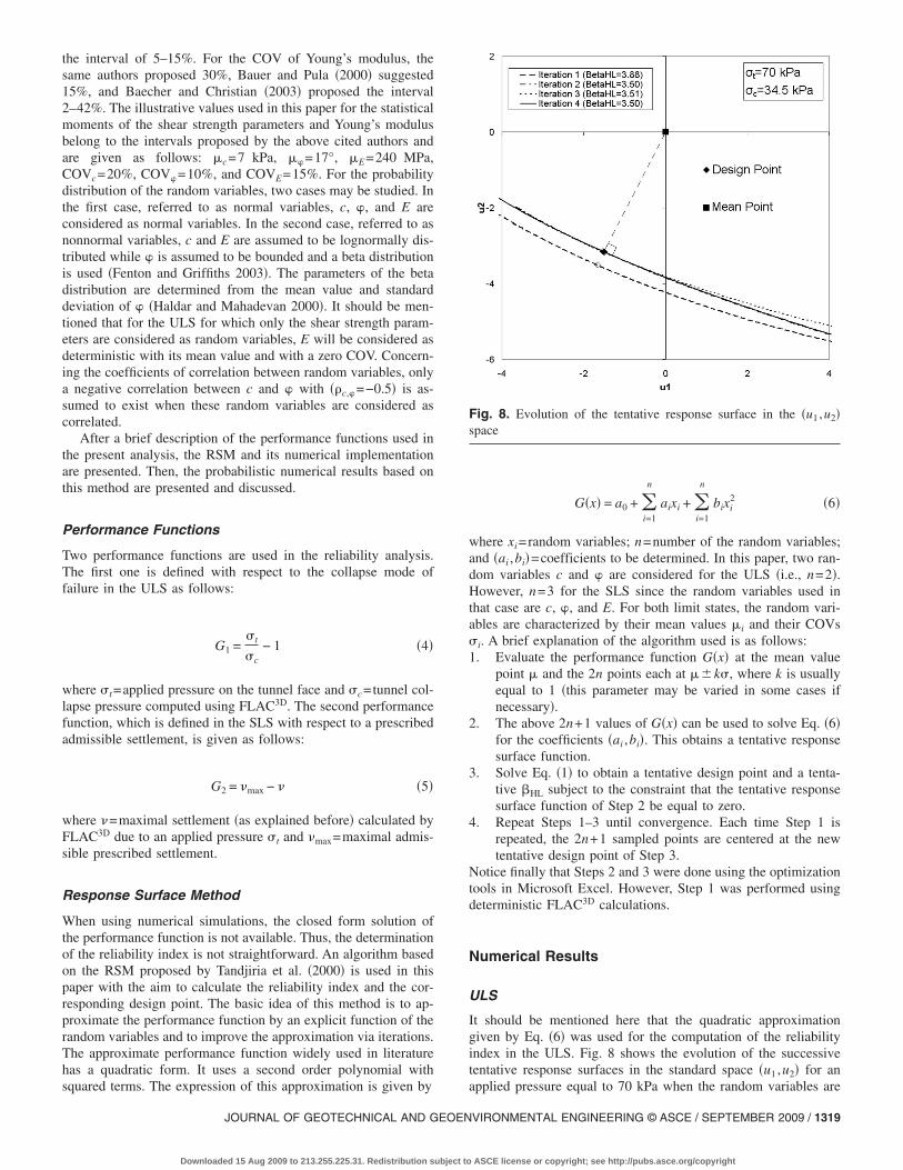
It should be mentioned here that the quadratic approximationgiven by Eq. �6� was used for the computation of the reliabilityindex in the ULS. Fig. 8 shows the evolution of the successivetentative response surfaces in the standard space �u1 ,u2� for an

Fig. 8. Evolution of the tentative response surface in the �u1 ,u2�space

applied pressure equal to 70 kPa when the random variables are



assumed normal and uncorrelated. A convergence criterion on thereliability index was adopted. It considers that convergence isreached when a difference �in absolute value� smaller than 10−2

between two successive reliability indexes is achieved. One cannotice that this criterion is reached after three to five iterations.Thus, only 15–25 numerical simulations by FLAC3D were neces-sary. The corresponding CPU time required is about 2090 min=1,800 min �i.e., 30 h�. A value of 3.50 was found forthe reliability index in the case of uncorrelated ��c,�=0� variablesand a value of 4.47 for correlated ��c,�=−0.5� variables. Thesevalues correspond to failure probabilities of 2.310−4 and 4.010−6 as calculated by FORM approximation.

Fig. 9 shows a comparison between the reliability results �re-

Table 2. Reliability Index and Design Point for ULS for Normal, Nonno

�t

�kPa�

�c,�=0.0

c�

�kPa� �� degrees� �HL Fc

�a� Nor

34.5 7.00 17.00 0.000 1.00

40 6.44 15.94 0.740 1.09

50 5.71 14.36 1.816 1.23

60 5.23 12.89 2.736 1.34

70 4.89 11.63 3.502 1.43

80 4.67 10.46 4.199 1.50

�b� Nonn

34.8 7.00 17.00 0.000 1.00

40 6.40 15.97 0.691 1.09

50 5.82 14.25 1.847 1.20

60 5.42 12.79 2.858 1.29

70 5.17 11.46 3.784 1.35

80 4.92 10.35 4.626 1.42

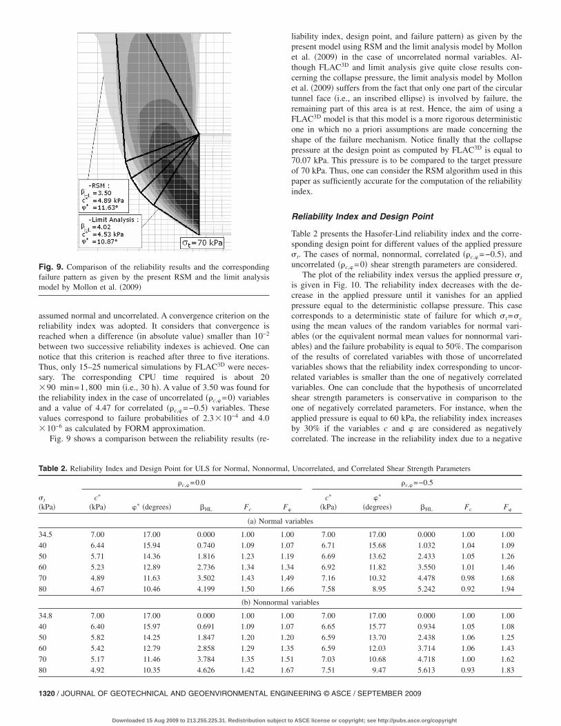
Fig. 9. Comparison of the reliability results and the correspondingfailure pattern as given by the present RSM and the limit analysismodel by Mollon et al. �2009�



liability index, design point, and failure pattern� as given by thepresent model using RSM and the limit analysis model by Mollonet al. �2009� in the case of uncorrelated normal variables. Al-though FLAC3D and limit analysis give quite close results con-cerning the collapse pressure, the limit analysis model by Mollonet al. �2009� suffers from the fact that only one part of the circulartunnel face �i.e., an inscribed ellipse� is involved by failure, theremaining part of this area is at rest. Hence, the aim of using aFLAC3D model is that this model is a more rigorous deterministicone in which no a priori assumptions are made concerning theshape of the failure mechanism. Notice finally that the collapsepressure at the design point as computed by FLAC3D is equal to70.07 kPa. This pressure is to be compared to the target pressureof 70 kPa. Thus, one can consider the RSM algorithm used in thispaper as sufficiently accurate for the computation of the reliabilityindex.

Reliability Index and Design Point

Table 2 presents the Hasofer-Lind reliability index and the corre-sponding design point for different values of the applied pressure�t. The cases of normal, nonnormal, correlated ��c,�=−0.5�, anduncorrelated ��c,�=0� shear strength parameters are considered.

The plot of the reliability index versus the applied pressure �t

is given in Fig. 10. The reliability index decreases with the de-crease in the applied pressure until it vanishes for an appliedpressure equal to the deterministic collapse pressure. This casecorresponds to a deterministic state of failure for which �t=�c

using the mean values of the random variables for normal vari-ables �or the equivalent normal mean values for nonnormal vari-ables� and the failure probability is equal to 50%. The comparisonof the results of correlated variables with those of uncorrelatedvariables shows that the reliability index corresponding to uncor-related variables is smaller than the one of negatively correlatedvariables. One can conclude that the hypothesis of uncorrelatedshear strength parameters is conservative in comparison to theone of negatively correlated parameters. For instance, when theapplied pressure is equal to 60 kPa, the reliability index increasesby 30% if the variables c and � are considered as negativelycorrelated. The increase in the reliability index due to a negative

Uncorrelated, and Correlated Shear Strength Parameters

�c,�=−0.5

c�

�kPa��

�degrees� �HL Fc F�

riables

7.00 17.00 0.000 1.00 1.00

6.71 15.68 1.032 1.04 1.09

6.69 13.62 2.433 1.05 1.26

6.92 11.82 3.550 1.01 1.46

7.16 10.32 4.478 0.98 1.68

7.58 8.95 5.242 0.92 1.94

variables

7.00 17.00 0.000 1.00 1.00

6.65 15.77 0.934 1.05 1.08

6.59 13.70 2.438 1.06 1.25

6.59 12.03 3.714 1.06 1.43

7.03 10.68 4.718 1.00 1.62

7.51 9.47 5.613 0.93 1.83

rmal,

F�

mal va

1.00

1.07

1.19

1.34

1.49

1.66

ormal

1.00

1.07

1.20

1.35

1.51

1.67



correlation may be explained with the aid of Fig. 11 in which thecritical ellipse corresponding to a negative correlation is greaterthan that of no correlation. The reliability index of nonnormalvariables is slightly greater than that of normal variables. For thesame pressure of 60 kPa, the reliability index increases by only5% if the variables are considered as nonnormal. The observationthat both normal and nonnormal variables give close results maybe explained by the fact that the cumulative distribution functionsof normal and nonnormal variables are practically similar in thezone of interest to the engineers corresponding to the differentdesign points obtained in the paper �these curves are not shown inthe paper�.

The values of the design points corresponding to different val-ues of the applied pressure can give an idea about the partialsafety factors of each of the strength parameters c and tan � asfollows:

Fc =�c

c��7�

F� =tan��tan ��

�8�

Table 2 shows that for uncorrelated shear strength parameters, thevalues of c� and �� at the design point are smaller than theirrespective mean values and decrease with the increase in the ap-

Fig. 10. �HL versus applied pressure �t

Limit state surface

Design points

( )* *,c ϕ

c

ϕ

ϕµ

, 0=c ϕρ

, 0<c ϕρ

, 0>c ϕρ

Safe domain

Failure domain

cµ

Fig. 11. General layout of the critical dispersion ellipse for differentvalues of the correlation coefficient



plied pressure. Consequently, the partial safety factors Fc and F�

decrease with the decrease in the applied pressure. They tend to 1when �t=�c. For negatively correlated shear strength parameters,c� slightly exceeds the mean for some values of the applied pres-sure. This can be explained by the counterclockwise rotation ofthe critical dispersion ellipse due to the negative correlation �cf.Fig. 11�. The position of the design point, which is the point oftangency between the critical ellipse and the limit state surface,changes from the one found for uncorrelated soil shear strengthparameters. A higher value of c� and a lower value of �� werefound in the case of negative correlation. Consequently, c� canbecome greater than the mean value for a negative correlation.This conclusion is similar to that found by Youssef Abdel Massihand Soubra �2008�.

SLS

The classical RSM used before in the ULS was found not conve-nient in the present case of the SLS. Two issues were encoun-tered:1. It was impossible to compute a settlement for some sampling

points after a given number i of iterations. This is becausethese cases lead to a collapse of the tunnel face. This oc-curred when calculating the settlement corresponding topoints such as �ci−�c ,�i ,Ei� or �ci ,�i−�� ,Ei� for which asmaller value of ci or �i was considered for the settlementcomputations.

2. It was found that the successive iterations of the RSM do notconverge to a design point when using a quadratic approxi-mation for the limit state surface. Another form of this limitstate function was necessary as will be seen later.

The first issue may be explained with the aid of Fig. 12�a�.This figure shows the seven sampling points projected on a �c ,��plane. Thus, only five points are visible in that figure. It can beeasily seen that some sampling points can lead to a collapse of thetunnel face since they correspond to shear strength parameterslocated in the failure zone of the �c ,�� plane as defined in theULS study. Two different ways may be used to overcome thisissue. The first one consists in reducing the k value defined in theRSM, as shown in Fig. 12�b�. This resolves the collapse issue forall the sampling points but unfortunately it does not lead to con-vergence. This is because the approximation of the limit statesurface was not accurate in this case; this surface being based onvery neighboring sampling points. A second and more efficientmethod is proposed in Fig. 12�c� where the shear strength param-eters are chosen in a nonsymmetrical manner with respect to thecentral point. Thus, the seven sampling points used for the deter-mination of the limit state surface approximation become�ci ,�i ,Ei�, �ci+1.2�c ,�i ,Ei�, �ci−0.3�c ,�i ,Ei�, �ci ,�i+1.4�� ,Ei�,�ci ,�i−0.3�� ,Ei�, �ci ,�i ,Ei+�E�, and �ci ,�i ,Ei−�E�. This choiceof the sampling points was made arbitrarily. It prevents the facecollapse �by not reducing too much the value of c and ��. Itslightly shifts the sampling points to the safe domain. However,these points remain close to the limit state surface in order toobtain a good approximation of this surface. Notice finally thatthe choice of the values of k has a small influence on the results.The sampling points can thus be located anywhere in the neigh-borhood of the design point. This method will be used in allsubsequent SLS simulations.

The second issue is due to the use of a quadratic approxima-tion for the limit state surface. In the present case of the SLS, this
approximation was found not convenient since it does not make


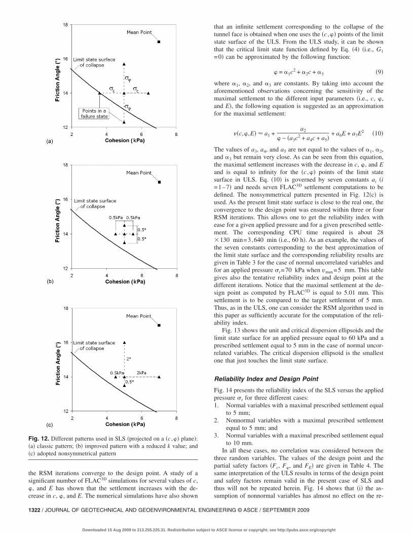
the RSM iterations converge to the design point. A study of asignificant number of FLAC3D simulations for several values of c,�, and E has shown that the settlement increases with the de-

Fig. 12. Different patterns used in SLS �projected on a �c ,�� plane�:�a� classic pattern; �b� improved pattern with a reduced k value; and�c� adopted nonsymmetrical pattern

crease in c, �, and E. The numerical simulations have also shown



that an infinite settlement corresponding to the collapse of thetunnel face is obtained when one uses the �c ,�� points of the limitstate surface of the ULS. From the ULS study, it can be shownthat the critical limit state function defined by Eq. �4� �i.e., G1

=0� can be approximated by the following function:

� = 1c2 + 2c + 3 �9�

where 1, 2, and 3 are constants. By taking into account theaforementioned observations concerning the sensitivity of themaximal settlement to the different input parameters �i.e., c, �,and E�, the following equation is suggested as an approximationfor the maximal settlement:

��c,�,E� � a1 +a2

� − �a3c2 + a4c + a5�+ a6E + a7E2 �10�

The values of a3, a4, and a5 are not equal to the values of 1, 2,and 3 but remain very close. As can be seen from this equation,the maximal settlement increases with the decrease in c, �, and Eand is equal to infinity for the �c ,�� points of the limit statesurface in ULS. Eq. �10� is governed by seven constants ai �i=1–7� and needs seven FLAC3D settlement computations to bedefined. The nonsymmetrical pattern presented in Fig. 12�c� isused. As the present limit state surface is close to the real one, theconvergence to the design point was ensured within three or fourRSM iterations. This allows one to get the reliability index withease for a given applied pressure and for a given prescribed settle-ment. The corresponding CPU time required is about 28130 min=3,640 min �i.e., 60 h�. As an example, the values ofthe seven constants corresponding to the best approximation ofthe limit state surface and the corresponding reliability results aregiven in Table 3 for the case of normal uncorrelated variables andfor an applied pressure �t=70 kPa when vmax=5 mm. This tablegives also the tentative reliability index and design point at thedifferent iterations. Notice that the maximal settlement at the de-sign point as computed by FLAC3D is equal to 5.01 mm. Thissettlement is to be compared to the target settlement of 5 mm.Thus, as in the ULS, one can consider the RSM algorithm used inthis paper as sufficiently accurate for the computation of the reli-ability index.

Fig. 13 shows the unit and critical dispersion ellipsoids and thelimit state surface for an applied pressure equal to 60 kPa and aprescribed settlement equal to 5 mm in the case of normal uncor-related variables. The critical dispersion ellipsoid is the smallestone that just touches the limit state surface.

Reliability Index and Design Point

Fig. 14 presents the reliability index of the SLS versus the appliedpressure �t for three different cases:1. Normal variables with a maximal prescribed settlement equal

to 5 mm;2. Nonnormal variables with a maximal prescribed settlement

equal to 5 mm; and3. Normal variables with a maximal prescribed settlement equal

to 10 mm.In all these cases, no correlation was considered between the

three random variables. The values of the design point and thepartial safety factors �Fc, F�, and FE� are given in Table 4. Thesame interpretation of the ULS results in terms of the design pointand safety factors remain valid in the present case of SLS andthus will not be repeated herein. Fig. 14 shows that �i� the as-
sumption of nonnormal variables has almost no effect on the re-




liability index for �t�60 kPa as in the ULS case and �ii� aprescribed settlement of 10 mm instead of 5 mm increases thereliability index; the increase is equal to 16% when �t=70 kPa.

Comparison between the Two Limit States

Fig. 15 shows a comparison between the values of �HL given bythe ULS and the SLS �in both cases of �max=5 mm and �max

=10 mm�. The reliability index of both limit states have almostthe same evolution versus the applied pressure. This may be ex-plained by the fact that both limit states are controlled by thesame parameters �mainly c and �� and correspond to the samephysical phenomenon: the occurrence of a settlement can be con-sidered as the beginning of a failure state because it implies plas-tic deformations around the tunnel face. Finally, from Fig. 15, onecan easily see that the reliability index against face collapse andthe one against a 10-mm maximal settlement are almost the same.

Table 5 gives the components and the system reliability indexof both limit states. The equations used are given in YoussefAbdel Massih and Soubra �2008� and are not repeated herein. Thecoefficient of correlation between the two limit states was foundvery close to 1 �0.97��ULS-SLS�1� for the different applied pres-sures. This indicates a strong positive correlation between bothlimit states and confirms the observation made above concerningthe evolution of both limit states in the same manner. It was alsofound that the system reliability index depends on both limitstates. It is smaller than the reliability index corresponding to asingle failure mode but it is very close to the one of SLS. It isequal to that of SLS for high values of the applied pressure.

and �max=5 mm�

2 3 4

2.909 2.897 2.903

5.41 5.58 5.51

12.65 12.48 12.50

211.25 220.94 220.94

surface at the fourth iteration:=14.75; a6=−0.0684; and a7=0.000103

Fig. 14. Reliability index versus applied pressure �t for SLS

Table 3. Design Point along the Different RSM Iterations for SLS ��t=70 kPa

RSM iteration number �i� Mean point 1

BHLi 0 3.685

ci �kPa� 7 5.22

�i �deg� 17 11.28

Ei �MPa� 240 211.05

Best approximation of the limit statea1=11.67; a2=5.20; a3=0.0357; a4=−0.882; a5

Fig. 13. Graphical representation of unit and critical dispersion el-lipsoids for SLS: �a� in the three-dimensional space; �b� projected onthe planes c=c� and E=E�



Hence, the contribution of ULS to the system reliability is notsignificant. As a conclusion, SLS can be used alone for the as-sessment of the tunnel reliability.

Conclusions

A reliability-based analysis of a shallow circular tunnel driven bya pressurized shield in a c−� soil is presented. Both the ULS andthe SLS are considered in the analysis. Two deterministic modelsbased on numerical simulations using the Lagrangian explicitfinite-difference code FLAC3D are employed. The first one com-putes the collapse pressure of the tunnel face and the second onecalculates the maximal settlement due to a given applied pressureon the tunnel face. In both models, the stress control method is

Table 4. Reliability Index and Design Point for SLS for Normal and No

�t

�kPa�c�

�kPa��

�deg�E�

�MPa�

�a� Normal variables, max

40 6.90 16.87 239.25

50 6.32 15.26 230.16

60 5.88 13.80 222.95

70 5.51 12.50 220.94

80 5.16 11.39 213.53

�b� Nonnormal variables, m

40 6.85 16.92 237.07

50 6.29 15.31 227.79

60 5.93 13.82 220.22

70 5.62 12.53 213.40

80 5.38 11.33 208.99

�c� Normal variables, max

40 6.54 16.00 239.20

50 5.99 14.43 238.29

60 5.52 13.00 237.76

70 5.09 11.77 235.32

80 4.83 10.76 233.00

Fig. 15. Comparison between ULS and SLS



used. Concerning the assessment of the tunnel reliability, theHasofer-Lind reliability index is adopted here. The RSM is usedto find an approximation of the analytically unknown limit statesurfaces and the corresponding reliability indices. Only the soilshear strength parameters are considered as random variableswhile studying the ULS. However, the randomness of bothYoung’s modulus and the shear strength parameters of the soil istaken into account in the SLS. The main conclusions of this papercan be summarized as follows.

For the ULS, the hypothesis of uncorrelated shear strengthparameters was found conservative in comparison to the one ofnegatively correlated variables. For uncorrelated shear strengthparameters, the values of c� and �� at the design point are foundsmaller than their respective mean values and increase with thedecrease in the applied pressure �t. Consequently, the partialsafety factors Fc and F� decrease with the decrease in the appliedpressure. They tend to 1 when �t=�c. For negatively correlatedshear strength parameters, c� slightly exceeds the mean for somevalues of the applied pressure.

For the SLS, when the shear strength parameters are consid-ered as uncorrelated, the partial safety factors Fc, F�, and FE

decrease with the decrease in �t. They tend to 1 when �t is equalto the pressure that leads to the maximal prescribed settlement�max for the mean values of c, �, and E.

For both ULS and SLS, the assumption of nonnormal distri-

al Variables with No Correlation

�HL Fc F� FE

ettlement equal to 5 mm

0.109 1.01 1.01 1.00

1.165 1.11 1.12 1.04

2.098 1.19 1.24 1.08

2.903 1.27 1.38 1.10

3.628 1.36 1.52 1.12

l settlement equal to 5 mm

0.030 1.02 1.01 1.01

1.121 1.11 1.12 1.05

2.121 1.18 1.24 1.09

3.035 1.25 1.38 1.12

3.899 1.30 1.53 1.15

ttlement equal to 10 mm

0.673 1.07 1.07 1.00

1.676 1.17 1.19 1.01

2.500 1.27 1.32 1.01

3.367 1.38 1.47 1.02

4.031 1.45 1.61 1.03

Table 5. Reliability Index of the System ULS-SLS for �max=5 mm

�t

�kPa�

�HL

ULS SLSSystem

ULS-SLS

40 0.740 0.109 0.089

50 1.806 1.165 1.163

60 2.726 2.098 2.097

70 3.502 2.901 2.901

80 4.189 3.628 3.628

nnorm

imal s

axima

imal se



bution for the random variables has almost no effect on the reli-ability index for the practical range of values of the appliedpressure �t. The reliability index of both limit states follows thesame evolution with the increase in the applied pressure. Thismay be explained by the fact that both limit states are controlledby the same parameters �mainly c and �� and correspond to thesame physical phenomenon: the occurrence of a settlement can beconsidered as the beginning of a failure state because it impliesplastic deformations around the tunnel face.

It was found that the system reliability index depends on bothlimit states. It is smaller than the reliability index correspondingto a single failure mode but it is very close to the one of SLS. Itis equal to that of SLS for high values of the applied pressure.Hence, the contribution of ULS to the system reliability is notsignificant. As a conclusion, SLS can be used alone for the as-sessment of the tunnel reliability. It should be remembered herethat SLS in the present paper is based on the computation of thesettlement due to only the face pressure. In a future work, it issuggested to investigate a more sophisticated SLS deterministicmodel that considers an exhaustive analysis of the total settlementdue to the different construction parameters and to perform aprobabilistic analysis based on this unique limit state. The newprobabilistic SLS model can take advantage of the thoroughanalysis concerning �1� the shape of the response surface found inthe paper; and �2� the nonsymmetrical pattern of the samplingpoints since the influence of both c and � on the settlement isexpected to remain the same in the new sophisticated determinis-tic model.

References

Baecher, G. B., and Christian, J. T. �2003�. Reliability and statistics ingeotechnical engineering, Wiley.

Bauer, J., and Pula, W. �2000�. “Reliability with respect to settlementlimit-states of shallow foundations on linearly-deformable subsoil.”Comput. Geotech., 26�1�, 281–308.

Cherubini, C., Giasi, I., and Rethati, L. �1993�. “The coefficient of varia-tion of some geotechnical parameters.” Probabilistic methods in geo-technical engineering, K. S. Li and S.-C. R. Lo, eds., Balkema,Rotterdam, 179–183.

Dias, D., and Kastner, R. �2005�. “Modélisation numérique de l’apport durenforcement par boulonnage du front de taille des tunnels.” Can.Geotech. J., 42, 1656–1674 �in French�.

Dias, D., Kastner, R., and Dubois, P. �1997�. “Tunnel face reinforcementby bolting: Strain approach using 3D analysis.” Proc., Int. Conf. onTunneling under Difficult Conditions, Basel, Switzerland, Balkema,Rotterdam.

Dias, D., Kastner, R., and Jassionnesse, C. �2002�. “Sols renforcés parboulonnage. Etude numérique et application au front de taille d’untunnel profond.” Geotechnique, 52�1�, 15–27 �in French�.

Ditlevsen, O. �1981�. Uncertainty modeling: With applications to multi-dimensional civil engineering systems, McGraw-Hill, New York.

Eclaircy-Caudron, S., Dias, D., and Kastner, R. �2007�. “Inverse analysison measurements realized during a tunnel excavation.” Proc., ITA-AITES World Tunnel Congress 2007, Prague, Czech Republic, Barták
et al., eds.


Fenton, G. A., and Griffiths, D. V. �2003�. “Bearing capacity prediction ofspatially random C−� soils.” Can. Geotech. J., 40, 54–65.

FLAC3D. �1993�. Fast Lagrangian analysis of continua, ITASCA Con-sulting Group, Inc., Minneapolis.

Haldar, A., and Mahadevan, S. �2000�. Probability, reliability, and statis-tical methods in engineering design, Wiley, New York.

Hasofer, A. M., and Lind, N. C. �1974�. “Exact and invariant second-moment code format.” J. Engrg. Mech. Div., 100�1�, 111–121.

Jardine, R. J., Potts, D. M., Fourie, A. B., and Burland, J. B. �1986�.“Studies of the influence of nonlinear stress strain characteristics insoil-structure interaction.” Geotechnique, 36�3�, 377–396.

Jenck, O., and Dias, D. �2003�. “Numerical analysis of the volume lossinfluence on building during tunnel excavation.” Proc., 3rd Int. FLACSymp.—FLAC and FLAC3D Numerical Modeling in Geomechanics,Sudbury, Ontario, Canada, C. Detournay and R. Hart, eds.

Jenck, O., and Dias, D. �2004�. “Analyse tridimensionnelle en différencesfinies de l’interaction entre une structure en béton et le creusementd’un tunnel à faible profondeur.” Geotechnique, 54�8�, 519–528 �inFrench�.

Low, B. K. �2005�. “Reliability-based design applied to retaining walls.”Geotechnique, 55�1�, 63–75.

Low, B. K., and Tang, W. H. �1997a�. “Efficient reliability evaluationusing spreadsheet.” J. Eng. Mech., 123�7�, 749–752.

Low, B. K., and Tang, W. H. �1997b�. “Reliability analysis of reinforcedembankments on soft ground.” Can. Geotech. J., 34, 672–685.

Low, B. K., and Tang, W. H. �2004�. “Reliability analysis using object-oriented constrained optimization.” Struct. Safety, 26, 69–89.

Mollon, G., Dias, D., and Soubra, A.-H. �2009�. “Probabilistic analysisand design of circular tunnels against face stability.” Int. J. Geomech.,in press.

Mroueh, H., and Shahrour, I. �2003�. “A full 3-D finite element analysisof tunneling-adjacent structures interaction.” Computers and Geotech-nics, 30, 245–253.

Phoon, K.-K., and Kulhawy, F. H. �1999�. “Evaluation of geotechnicalproperty variablity.” Can. Geotech. J., 36, 625–639.

Potts, D. M., and Addenbrooke, T. I. �1997�. “A structure’s influence ontunneling induced ground movements.” Geotech. Eng., 125�2�, 109–125.

Ribeiro e Sousa, L., Dias, D., and Barreto, J. �2003�. “Lisbon metroyellow line extension. Structural behavior of the Ameixoeira station.”Proc., 12th Panamerican Conf. on Soil Mechanics and GeotechnicalEngineering, Boston, Verlag Glückauf Gmbh, eds.

Tandjiria, V., Teh, C. I., and Low, B. K. �2000�. “Reliability analysis oflaterally loaded piles using response surface methods.” Struct. Safety,22, 335–355.

Vanoudheusden, E. �2006�. “Impact de la construction de tunnels urbainssur les mouvements de sol et le bâti existant—Incidence du mode depressurisation du front.” Ph.D. thesis, INSA Lyon, Lyon, France �inFrench�.

Wong, H., Subrin, D., and Dias, D. �2006�. “Convergence-confinementanalysis of a bolt-supported tunnel using homogenization method.”Can. Geotech. J., 43�5�, 462–483.

Yoo, C. S. �2002�. “Finite-element analysis of tunnel face reinforced bylongitudinal pipes.” Computers and Geotechnics, 29�1�, 73–94.

Youssef Abdel Massih, D. S., and Soubra, A.-H. �2008�. “Reliability-based analysis of strip footings using response surface methodology.”Int. J. Geomech., 8�2�, 134–143.

Youssef Abdel Massih, D. S., Soubra, A.-H., and Low, B. K. �2008�.“Reliability-based analysis and design of strip footings against bear-
ing capacity failure.” J. Geotech. Geoenviron. Eng., 134�7�, 917–928.


probabilistic analysis of circular tunnels in...

Documents