private alternating least squares: practical private
TRANSCRIPT
Private Alternating Least Squares:Practical Private Matrix Completion with Tighter Rates
Steve Chien 1 Prateek Jain 1 Walid Krichene * 1 Steffen Rendle 1
Shuang Song 1 Abhradeep Thakurta * 1 Li Zhang 1
Abstract
We study the problem of differentially private(DP) matrix completion under user-level privacy.We design a joint differentially private variantof the popular Alternating-Least-Squares (ALS)method that achieves: i) (nearly) optimal sam-ple complexity for matrix completion (in terms ofnumber of items, users), and ii) the best known pri-vacy/utility trade-off both theoretically, as well ason benchmark data sets. In particular, we providethe first global convergence analysis of ALS withnoise introduced to ensure DP, and show that, incomparison to the best known alternative (the Pri-vate Frank-Wolfe algorithm by Jain et al. (2018)),our error bounds scale significantly better withrespect to the number of items and users, whichis critical in practical problems. Extensive vali-dation on standard benchmarks demonstrate thatthe algorithm, in combination with carefully de-signed sampling procedures, is significantly moreaccurate than existing techniques, thus promisingto be the first practical DP embedding model.
1. IntroductionGiven M ij , (i, j) ∈ Ω where Ω ⊆ [n]× [m] is a set of ob-served user-item ratings, and assuming M ≈ U∗(V ∗)> ∈Rn×m to be a nearly low-rank matrix, the goal of low-rankmatrix completion (LRMC) is to efficiently learn U ∈ Rn×rand V ∈ Rm×r, such that M ≈ U V >.
LRMC, a.k.a. matrix factorization, is a cornerstone tech-nique for building recommendation systems (Koren & Bell,2015; Hu et al., 2008), and though proposed over a decadeago, it remains highly competitive (Rendle et al., 2019).In the recommendation setting, M represents a mostly un-
1Google Research. Correspondence to: WalidKrichene <[email protected]>, Abhradeep Thakurta<[email protected]>.
Proceedings of the 38 th International Conference on MachineLearning, PMLR 139, 2021. Copyright 2021 by the author(s).
known user-item ratings matrix and U and V capture theuser and item embeddings. Using the learned (U , V ), thesystem computes rating predictions M ij = (U V >)ij torecommend items for the users. To ensure good generaliza-tion, one would set the rank r min(m,n).
Such models, while highly successful in practice, have therisk of leaking users’ ratings through model parameters ortheir recommendations. The privacy risk of similar modelshas been well documented, and the protection against it hasbeen intensively studied (Dinur & Nissim, 2003; Dworket al., 2007; Korolova, 2010; Calandrino et al., 2011; Shokriet al., 2017; Carlini et al., 2019; 2020a;b; Thakkar et al.,2020). In this paper, we focus on learning user and itemembeddings, and consequently user-item recommendations,while ensuring privacy of users’ ratings.
We conform to the well-established formal notion of dif-ferential privacy (DP) (Dwork et al., 2006a;b) to protectusers’ ratings. We operate in the setting of user-level pri-vacy (Dwork & Roth, 2014; Jain et al., 2018), where we in-tend to protect all the ratings by the user, a much harder taskthan protecting a single rating from the user (a.k.a. entry-level privacy) (Hardt & Roth, 2013; Meng et al., 2018).Note that user-level privacy is critical in this problem, asthe ratings from a single user tend to be correlated and canthus be used to fingerprint a user (Calandrino et al., 2011).As is standard in the user-level privacy literature (Jain et al.,2018), we estimate the shared item embeddings V whilepreserving privacy with respect to the users. In contrast,each user independently computes their embedding (a rowof U ) as a function of their own ratings and the privacypreserving item embeddings V . Formally, this setup iscalled joint differential privacy (Kearns et al., 2014), and itis well-established (Hardt & Roth, 2012; 2013) that such arelaxation is necessary to learn non-trivial recommendationswhile ensuring user-level privacy.
While several works have studied LRMC under joint-differential privacy (McSherry & Mironov, 2009; Liu et al.,2015; Jain et al., 2018), most of the existing techniques donot provide satisfactory empirical performance comparedto the state-of-the-art (SOTA) non-private LRMC methods.Furthermore, these works either lack a rigorous performance
arX
iv:2
107.
0980
2v1
[cs
.LG
] 2
0 Ju
l 202
1

Private Alternating Least Squares
analysis (McSherry & Mironov, 2009; Liu et al., 2015) orprovide guarantees that are significantly weaker (Jain et al.,2018) than that of non-private LRMC algorithms. Matrixfactorization can also be solved using other first-order meth-ods such as stochastic gradient descent (Ge et al., 2016)or alternating gradient descent (Lu et al., 2019), so onemay apply the differentially private SGD (DPSGD) algo-rithm (Song et al., 2013; Bassily et al., 2014; Abadi et al.,2016) to achieve privacy. However, applying DPSGD toLRMC is challenging as SGD typically requires many stepsto converge, thus increasing privacy cost.
In this work, we design and analyze a differentially pri-vate version of the widely used alternating least squares(ALS) algorithm for LRMC (Koren et al., 2009; Jain et al.,2013). ALS alternates between optimizing over the userembeddings U and the item embeddings V , each throughleast squares minimization. One important property of ALSis that when solving for one side, the optimization can bedone independently for each user or item, which makes ALShighly scalable. Our key insight is that this decoupling of thesolution is also useful for privacy-preserving computation,since there is no accumulation of noise when solving for theembeddings of different users (or items). Besides, ALS isknown to require few iterations to converge in practice, mak-ing it particularly suitable for privacy preserving LRMC.
Indeed, we present a differentially private variant of ALS,which we refer to as DPALS, and demonstrate that it enjoysmuch tighter error rates (see Table 1) and better empiricalperformance than the current SOTA, the differentially pri-vate Frank-Wolfe (DPFW) method of Jain et al. (2018). Fur-thermore, on the large scale benchmark of MovieLens 20M,DPALS produces the first realistic DP embedding modelwith competitive recall metric under moderate privacy loss.
More specifically, our contributions are the following.
Private alternating least squares for matrix completion.We provide the first differentially private version of alter-nating least squares (DPALS) for matrix completion withuser-level privacy guarantee (Section 3). The algorithm isconceptually simple, efficient, and highly scalable. We pro-vide rigorous analysis on its privacy guarantee under thenotion of Joint Renyi Differential Privacy.
Initizlization via noisy power iteration. For convergenceof DPALS algorithm, we need it to be initialized with aV
0close to V ∗ in spectral norm. The standard approach
based on private PCA (Dwork et al., 2014) would requiren = Ω
(m√mε
)to achieve the initialization condition. In-
stead, we show that with a careful analysis, initializingwith noisy power iteration only requires n = Ω
(mε
). Our
analysis shows in particular that it suffices that the top-reigenspace of A := PΩ(M)>PΩ(M) be incoherent, andthat there be a Ω(log2m) gap between the top-r eigenvalues
Table 1. Sample complexity bounds for various algorithms, assum-ing constant Frobenius norm error. Here, n is the number of users,m is the number of items, and Ω(·) hides polylog(n,m, 1/δ). (*)assumes additional property of M being incoherent.
Algorithm Bound on n Bound on |Ω|/n IterationsTrace Norm (*) (non-priv.)
(Candes & Recht, 2009) Ω(m) Ω(log2 n) poly(n,m)
ALS (*) (non-priv.) (Jain et al., 2013) Ω(m) Ω(log2 n) polylog(n,m)
Private SVD(*)(McSherry & Mironov, 2009) - - -
Private SGLD (Liu et al., 2015) - - -Private FW (Jain et al., 2018) Ω(m5/4) Ω(
√m) poly(n,m)
Private ALS (*) (this work) Ω(m) Ω(log3 n) polylog(n,m)
and the rest. This result improves on (Hardt & Price, 2013)which required all the eigenvectors of A to be incoherent, acondition that is hard to guarantee in our setting (Dekel et al.,2011; Vu & Wang, 2015; Rudelson & Vershynin, 2015).
Tighter privacy/utility/computation trade-offs. Weprove theoretical guarantees on the sample complexity andthe error bounds of DPALS under standard assumptions(Section 4). These bounds are much tighter than the cur-rent SOTA, the DPFW method (Jain et al., 2018). In par-ticular, we show the following. First, DPALS requiresonly O(logO(1) n) samples per user to guarantee its con-vergence. In contrast, DPFW requires
√m ratings per user.
Second, to achieve a Frobenius norm error of ζ, DPALSrequires n = Ω
(m√m
ζε +m)
users, which is nearly op-timal in terms of ζ and ε. In contrast, DPFW’s samplecomplexity is n = Ω
(m5/4/(ζ5ε)
); note a significant im-
provement in terms of ζ. Finally, Private SVD (McSherry& Mironov, 2009) is not even consistent, i.e., for a fixedε,m, |Ω| = n
√m, even if we scale n→∞, the Frobenius
norm error bound does not converge to 0 (see Theorem B.3of Jain et al. (2018)).
Practical techniques to improve accuracy. One main dif-ficulty in applying DPALS to practical problems comesfrom a heavy skew in the item distribution. We propose twoheuristics to reduce the skew while preserving privacy (Sec-tion 5). Experiments on real-world benchmarks show thatthese techniques can significantly improve model quality.
Strong empirical results using DPALS. We carry out anextensive study of DPALS on synthetic and real-worldbenchmarks. Aided by the aforementioned practical tech-niques, DPALS achieves significant gains over the currentSOTA method. In particular, on the MovieLens 10M ratingprediction benchmark, DPALS achieves the same error rateas the current SOTA even when trained on a fraction (23%)of users. When trained on all users, it achieves a relativedecrease in RMSE of at least 7%. DPALS also achievesremarkably good performance on the MovieLens 20M itemrecommendation benchmark with modest privacy loss, andremains competitive even with non-private ALS, the first DPprivate embedding model to achieve such strong results.

Private Alternating Least Squares
2. Background2.1. Notation
Let [m] denote the set 1, 2, · · · ,m. Let Rn×m denote theset of n×m matrices. Throughout the paper, we use boldface uppercase letters to represent matrices and lowercaseletters for vectors. For any matrix A = (Aij) ∈ Rn×m, letAi be the i-th row vector of A. Denote by ‖A‖F , ‖A‖∞the Frobenius norm and the max norm of A. For Ω ⊆ [n]×[m], define the projection PΩ(A) ∈ Rn×m as PΩ(A)ij =Aij if (i, j) ∈ Ω and 0 otherwise. For i ∈ [n], defineΩi := j : (i, j) ∈ Ω. Similarly, for j ∈ [m], let Ωj =i : (i, j) ∈ Ω. For u,v ∈ Rr, we use u ·v ∈ R to denotetheir dot product, and u⊗ v ∈ Rr×r for their outer product.
2.2. Matrix Completion, Alternating Least Squares
Let M ∈ Rn×m be a rank r matrix, such that each entryM ij (i ∈ [n], j ∈ [m]) represents the preference/affinity ofuser i for item j. Given a set of observed entries PΩ(M),Ω ⊆ [n]× [m], the goal of LRMC is to reconstruct M withminimal error. This can be achieved by finding U ∈ Rn×rand V ∈ Rm×r such that the regularized squared error‖PΩ
(M − U V >
)‖2F + λ‖U‖2F + λ‖V ‖2F is minimized.
This minimization problem is NP-hard in general (Hardtet al., 2014). But the alternating least squares (ALS) algo-rithm has proved to work well in practice.
ALS alternatingly computes U , V by minimizing the aboveobjective while assuming the other embeddings fixed. Eachstep can be solved efficiently through the standard leastsquares algorithm with the following closed form solution.
∀i Ut
i = (λI +∑j∈Ωi
Vt
j ⊗ Vt
j)−1∑j∈Ωi
M ijVt
j , (1)
∀j Vt+1
j = (λI +∑i∈Ωj
Ut
i ⊗ Ut
i)−1∑i∈Ωj
M ijUt
i. (2)
While ALS does not guarantee convergence to the globaloptimum in general, it works remarkably well in practiceand often produces U and V such that U V > is a goodapproximation of M . The practical success of ALS has in-spired many theoretical analyses, which make the followingadditional assumptions on M and Ω.
Assumption 1 (µ-incoherence). Let M = U∗Σ∗(V ∗)>
be the singular value decomposition of M , i.e. U∗ ∈Rn×r,V ∗ ∈ Rm×r are orthonormal matrices, and Σ∗ ∈Rr×r is the diagonal matrix of the singular values of M .We assume that M is µ-incoherent, that is, ∀i ∈ [n],‖U∗i ‖2 ≤
µ√r√n
; and ∀j ∈ [m],∥∥V ∗j∥∥2
≤ µ√r√m
.
Assumption 2 (Random Ω). We assume that Ω are randomobservations with probability p, that is, Ω = (i, j) ∈[n]× [m] : δij = 1, where δij ∈ 0, 1 are i.i.d. randomvariables with Pr[δij = 1] = p.
Jain et al. (2013); Hardt & Wootters (2014) showed that ALSconverges to M with high probability if M is µ-incoherentand p = Ω
(lognm
), where n ≥ m and Ω hides polynomial
dependence on µ, r, and the condition number of M . In thiswork, we make the same assumptions on M and Ω. Ourkey theoretical contribution is a similar convergence resultfor DPALS, under the additional requirements of user-leveldifferential privacy.
2.3. Joint Differential Privacy
Differential privacy (Dwork et al., 2006b;a) is a widelyadopted privacy notion. We use the variant of user-leveljoint differential privacy (Joint DP). Intuitively, Joint DPrequires any information which may cross different usersto be differentially private, but allows each individual userto use her own private information to her full advantage,for example, when computing the embeddings for generat-ing recommendations to herself. This notion was alreadyimplicit in (McSherry & Mironov, 2009) and made formalin (Kearns et al., 2014; Jain et al., 2018).
Let D = d1, . . . , dn be a data set of n records, whereeach sample di is drawn from a domain τ and belongs toindividual i (which we also refer to as a user). Let A :τ∗ → Sn be an algorithm that produces n outputs in somespace S, one for each user i. Let D−i be the data set withthe i-th user removed, and let A−i(D) be the set of outputswithout that of the i-th user. Also, let (di;D−i) be the dataset obtained by adding di (for user i) to the data set D−i.Joint DP and its Renyi differential privacy (Mironov, 2017)(Joint RDP) variant are defined as follows.Definition 3 (Joint Differential Privacy (Kearns et al.,2014)). An Algorithm A is (ε, δ)-jointly differentially pri-vate if for any user i, for any possible value of data entrydi, d
′i ∈ τ , for any instantiation of the data set for other
users D−i ∈ τn−1, and for any set of outputs S ⊆ Sn, thefollowing two inequalities hold simultaneously:
PrA
[A−i((di;D−i)) ∈ S] ≤ eε PrA
[A−i(D−i) ∈ S] + δ
PrA
[A−i(D−i) ∈ S] ≤ eε PrA
[A−i((di;D−i)) ∈ S] + δ.
An algorithm A is (α, ε)-joint Renyi differentially private(Joint RDP) if Dα (A−i((di;D−i))||A−i(D−i)) ≤ ε andDα (A−i(D−i)||A−i((di;D−i))) ≤ ε, where Dα is theRenyi divergence of order α.
If we replaceA−i withA in the definition, we would recoverthe standard definition of DP and RDP. We note that thejoint DP (resp. joint RDP) enjoys the same composabilityproperties as the notion of DP (resp. RDP).
3. DPALS: Private Alternating Least SquaresWe now provide the details of the DPALS algorithm andprove its privacy guarantee in the joint DP model.

Private Alternating Least Squares
Algorithm 1 DPALS: Private Matrix Completion via Alter-nating MinimizationRequired: PΩ(M): observed ratings, σ: noise standarddeviation, Γu: row clipping parameter, ΓM : entry clippingparameter, T : number of steps, λ: regularization parameter,r: rank, k: maximum number of ratings per user in Aitem ,V
0: initial V .
1 Clip entries in PΩ(M) so that ‖PΩ(M)‖∞ ≤ ΓM
for 0 ≤ t ≤ T dofor 1 ≤ i ≤ n do
2 Ut
i ← Auser (Vt,Ωi,PΩ(M)i, T, λ,Γu)
end3 U
t← [U
t
1, · · · , Ut
n]>
4 Vt+1← Aitem (U
t,Ω,PΩ(M), k, λ,Γu,ΓM )
end
5 return UT, V
T
Procedure Aitem (U , Ω, PΩ(M), k, λ, Γu, ΓM )6 Ω′ ← up to k random samples of (i, j) ∈ Ω, ∀i ∈ [n].
for 1 ≤ j ≤ m do7 Gj ← Nsym
(0,Γ4
u · σ2)r×r
8 gj ← N(0,Γ2
uΓ2M · σ2
)r9 Xj ← λI +
∑i∈Ω′j
U i ⊗U i + Gj
10 V j ← ΠPSD (Xj)+(∑
i∈Ω′jM ij ·U i + gj
)end
11 V = [V 1, · · · ,V m]>
12 return V = V (V>V )−1/2
Procedure Auser (V , Ωi, PΩ(M)i, T , λ, Γu)13 Ω′i ← random samples of 1/T fraction of j ∈ Ωi14 u← (λI +
∑j∈Ω′i
V j ⊗ V j)−1 ∑
j∈Ω′iM ijV j
15 return clip (u,Γu)
Notation. LetN (0, σ2) be the Gaussian distribution of vari-ance σ2, andNsym(0, σ2)r×r be the distribution of symmet-ric matrices where each entry in the upper triangle is drawni.i.d. from N (0, σ2). For a symmetric A, let ΠPSD (A)be its projection to the positive semi-definite cone, ob-tained by replacing its negative eigenvalues with 0. Defineclip (u, c) = u ·max(1, c/‖u‖2), i.e., the projection of uon an `2 ball of radius c. Let A+ be the pseudoinverse of A.
3.1. Algorithm
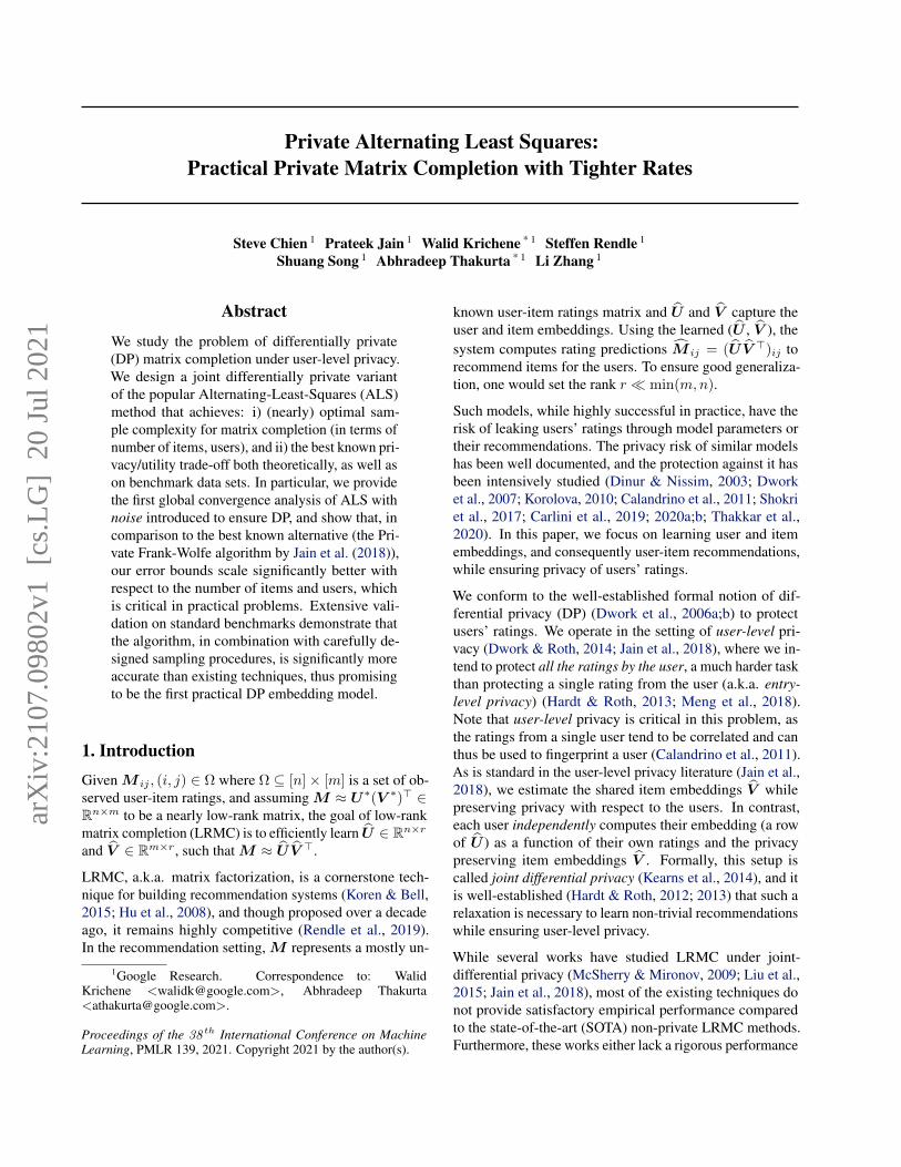
The private alternating least squares algorithm, DPALS,is described in Algorithm 1. It follows the standard ALSsteps, i.e. it alternatingly solves the least squares problemto obtain U and V using (1) and (2). To guarantee joint DP,we compute differentially private item embeddings V t+1
(using procedure Aitem ) by solving a private variant of (2),
User 1 User 2 User 𝑛Compute
$𝑼!" using ratings 𝑃# 𝑴 ! and $𝑽
Compute $𝑼$" using ratings 𝑃# 𝑴 $ and $𝑽
Compute $𝑼%" using ratings 𝑃# 𝑴 % and $𝑽
𝒜&'() 𝒜&'() 𝒜&'()
𝒜*+(,: Privately solve
argmin!𝑽||𝑃# 𝑴− +𝑼 +𝑽$ ||%& +𝑽
Output
Broadcast
......
Figure 1. Block schematic of Joint differentially private alternatingleast squares algorithm. Solid lines and boxes represent privilegedcomputations not visible to an adversary or other users. Dashedboxes and lines are public information accessible to anyone.
and compute each row of U t+1 independently without anynoise using procedure Auser . A block schematic of thealgorithm is presented in Figure 1.
Here we describe how the privacy is guaranteed in Aitem ;see Theorem 1 for a formal statement. For a given j ∈[m], write Ht
j = λI +∑i∈Ωj
U ti ⊗ U t
i and wtj =∑
i∈ΩjM ijU
ti. Then the non-private update (2) can be
written as V t+1j =
(Ht
j
)−1wtj . In the private version,
we need to add noise to protect both Htj and wt
j . To en-sure sufficient noise, we limit the influence of each user by“clipping” each U t
i to a bounded `2 norm Γu (Line 15 inAuser ) and resampling Ω such that each user participates inat most k items’ computation (Line 6 in Aitem ). We thenapply the Gaussian mechanism to Ht
j and wtj before using
them to compute V t+1j in Aitem (Lines 9–12).
While the above procedure is sufficient to guarantee privacy,we need a few additional modifications for utility analysis.
Initialization. Random initialization has worked well forour empirical study. For the utility analysis, we needV
0to be reasonably close to V ∗ (in terms of spectral
norm). We show that by using the noisy power iterationprocess, we are able to obtain V
0within the required bound
with n almost linear in m, an improvement compared toprivate PCA (Dwork et al., 2014), which would requiren = Ω(m
√m). See Section 4.1 for details.
Sampling from Ω. To ease the analysis, we require theobserved values to be independent across different steps.This is achieved by resampling from Ω at the beginning ofAitem (Line 6) and Auser (Line 13). The sampling in Aitem
is more important as it also limits the number of items peruser, for privacy purposes. In practice, we omit the samplingin Auser , and sample only once for Aitem . The samplingdistribution used in the latter has a significant impact inpractice, as discussed in Section 5.1.
Private Alternating Least Squares
3.2. Computational Complexity
The computational complexity of DPALS is comparable tothat of ALS. More precisely, the V step of ALS involvescomputing Ht
j and wtj , in O(|Ω′|r2), then solving the m
linear systems V t+1j =
(Ht
j
)−1wtj in O(mr3), for a total
complexity of O(|Ω′|r2 + mr3) (and similarly for the Ustep). This scales linearly in the number of observations |Ω′|and the number of items m. In the private version (Auser ),the only additional operations are forming the noise matri-ces (Lines 7–8) in O(mr2), and projecting Xj (Line 10), inO(mr3), so the complexity per iteration is the same as ALS.In comparison, the complexity of DPFW isO(Γ(m+ |Ω′|)),using Oja’s method. The per-iteration complexity also scaleslinearly in m and |Ω′|. Even though the per-iteration com-plexity of DPFW and DPALS are comparable, DPALS con-verges in much fewer iterations (see Appendix D.4 for anexample), which makes it more scalable in practice.
3.3. Privacy Guarantee
We now provide the privacy guarantee for DPALS. As eachsubroutine in DPALS is a variant of the Gaussian mecha-nism, we can apply the Renyi accounting (Mironov, 2017)and convert to (ε, δ)-DP. See Appendix A for the proof.
Theorem 1 (Privacy guarantee). Excluding the initializa-
tion of V0, Algorithm 1 is
(α, αρ2
)-joint RDP with ρ2 =
kT2σ2 . Hence for any ε > 0 and δ ∈ (0, 1), Algorithm 1 is
(ε, δ)-joint DP if we set σ =
√(2kT )(ε+log(1/δ))
ε .
The guarantee holds for all values of the parameters Γu,ΓM , T , λ, r, k. Note in particular that the scale of thenoise (Lines 7–8 in Algorithm 1) is normalized so that theexpression of σ in Theorem 1 does not depend on Γu, ΓM .
In the above guarantee, we have excluded the initializationprocess. With random initialization, which we use in prac-tice, there is no extra privacy cost. However, for the utilityguarantee, we need an extra DP procedure, detailed in Sec-tion 4.1, so that V
0is sufficiently close to V ∗. This can be
done within the same privacy bound as the main procedure.
4. Convergence Guarantee for DPALSWe now show that under standard low-rank matrix com-pletion assumptions (Assumptions 1 and 2), Algorithm 1,initialized with the noisy power method, solves the matrixcompletion problem. We will first present the results as-suming that V
0is close to V ∗. We will then present the
guarantee of the initialization procedure.
Theorem 2 (Utility guarantee). Suppose that M is a µ-incoherent rank-r matrix, and Ω consists of random ob-servations with probability p. Let σ∗1 ≥ · · ·σ∗r > 0 be the
singular values of M and κ := σ∗1/σ∗r its condition number.
There exists a universal constant C > 0, such that forall δ ∈ (0, 1), ε ∈ (0, log(1/δ)), if p ≥ µ6κ12r6 · log3 n
m
and√pn ≥ C
γ√
log(1/δ)
ε , where γ = Cκ6µ3r2√m ·
log2(κ · n), then DPALS, initialized with V0
s.t. ‖(I −V ∗(V ∗)>)V
0‖ ≤ C
κ2r2 logn , with parameters k = C ·
m · p log n, T = log(µκn/ε), σ =C√kT log(1/δ)
ε , Γu =Cµσ∗1
√r√
n, ΓM =
µ2rσ∗1√mn
and λ = 0, returns UT
and VT
such that the following holds:
• The distribution of (UT, V
T) satisfies (ε, δ)-joint DP.
• ‖M−UT
(VT
)>‖F ≤ C ·√m log(1/δ)
ε·n · κγ√p‖M‖F , withprobability ≥ 1− 1/n10.
• Similarly, ‖M − UT
(VT
)>‖∞ ≤ C ·√m log(1/δ)
ε·n · κγ√p ·µ2r‖M‖2√
mn, with probability ≥ 1− 1/n10.
Remark 1. The choice of hyper-parameters in Theorem 2assumes knowledge of certain quantities such as r, µ, κ. Inpractice, these quantities are unknown, but one can use stan-dard DP hyper-parameter search techniques (Liu & Talwar,2019) to search for optimal hyper-parameter values.Remark 2. The number of samples needed per user is aboutp ·m = O(µ6κ12r6 log3 n) which is nearly optimal withrespect to m and n. This represents a significant improve-ment over the DPFW algorithm in (Jain et al., 2018) whichrequires Ω(
√m) samples per user.
Remark 3. We did not optimize bounds for dependenceon the rank r and condition number κ. Prior work tends tofocus on the dependence on the size (m and n) and polyno-mial dependence on r, κ is common even in the non-privatesetting, for example (Jain et al., 2013; Sun & Luo, 2015;Ge et al., 2016). Our main goal is to provide a guarantee inthe private setting that is competitive with the non-privatesetting, so we inherit the focus on the size m,n. Further-more, dependence on κ can be removed (up to log factors)by using a stagewise ALS method similar to (Hardt & Woot-ters, 2014). However, this further complicates the proof andthe practical performance of standard ALS is comparable tosuch stagewise methods.Remark 4. Our Frobenius norm error bound is significantlysmaller than the bound for the DPFW algorithm, which is
given by ‖M−UT
(VT
)>‖F ≤(m5/4
nε
)1/5‖M‖F . In par-
ticular, to ensure an error ‖M − UT
(VT
)>‖F ≤ ζ‖M‖F ,DPALS requires n ≥ Cm
ζ·ε , while DPFW requires n ≥Cm5/4
ζ5·ε , which is significantly worse in terms of ζ. Fur-thermore, the DPFW bound is a generalization bound, i.e.,there is an additional bias term which can be large, and tothe best of our knowledge, existing techniques (even in thenon-private setting) require incoherence to control this term.
Private Alternating Least Squares
Remark 5. Consider a set of m linear regression problemsin r-dimensions:
y(i) = Xθ∗(i)
mi=1
, with X ∈ Rn×r.One can use a single iteration of DPALS with (U = X andPΩ(M) = [y(1), . . . ,y(m)]) to solve these linear regressionproblems. Assuming the conditions on M are satisfied, wecan obtain an excess empirical risk of O(
√m/(εn)). This
matches the best known upper bound for solving a set oflinear regressions with privacy (Sheffet, 2019; Smith et al.,2017). So, a better convergence rate of DPALS would leadto a tighter bound on solving a set of linear regressions witha common feature matrix. For m = O(1), we know that thelower bound for private linear regression is Ω(1/εn) (Smithet al., 2017). Thus, we conjecture that the error for DPALSis tight w.r.t. m and εn.Remark 6. Instead of using the perturbed objective func-tion to estimate V
tin DPALS, one can use DPSGD (Bassily
et al., 2014) to do the same (solving a least squares prob-lem with U
tfixed). We leave the empirical comparison of
this approach to future work. However, we know that forleast-square losses, perturbing the objective is known to betheoretically optimal (Smith et al., 2017).
Proof sketch: First, we show that under the assumptionsin Theorem 2, w.h.p., clipping and sampling operations inDPALS have no effect. Note, using k ≥ Cp ·m log n, w.p.≥ 1− 1/n100, ∀i, |Ωi| ≤ k. Furthermore, using Lemma 3,
‖Ut
i‖ ≤ Γu. Similarly, using Lemma 3, σmin(X) ≥ p/4−‖G‖2 ≥ p/4− Γ2
uσ√r ≥ p/8. That is, X 0.
The above observation implies that, under the assumptionsof the theorem, Algorithm 1 is essentially performing thefollowing iterative steps:i) U
t= arg min
U‖PΩ(M − U(V
t)>)‖2F , and
ii) Vt+1
j =(I+
∑i∈Ω′j
Ut
i⊗Ut
i+G)−1( ∑
i∈Ω′j
M ijUt
i+g)
.
Let U t (resp. V t) be the Q part in the QR decomposition ofUt
(resp. Vt). Using Lemma 4, we get Err(V ∗,V t+1) ≤
14Err(V ∗,V t) + α, where Err(V ∗,V ) = ‖(I −V ∗(V ∗)>)V ‖F and α ≤ Cκ6·µ3r2√logn√
pn
√m logn·T log 1/δ
ε .
That is, after T iterations, Err(V ∗,V T ) ≤ 2α. The secondclaim of the theorem now follows from the above observa-tion and Lemma 3. Similarly, the third claim follows byusing the bound on Err(V ∗,V T ) and incoherence of UT ,V T (Lemma 3). See Appendix B for a detailed proof.
Lemma 3. Suppose the assumptions of Theorem 2 hold.Then, w.p. ≥ 1 − 5T/n100, we have: a) each iterate U
t,
Vt
is 16κµ-incoherent, b) 1/2 ≤ σq(Ut(Σ∗)−1) ≤ 2 for
all q ∈ [r], c) 1/4 ≤ σq( 1p
∑i:(i,j)∈Ωv,t u
ti(u
ti)>) ≤ 4.
Lemma 4. Suppose the assumptions of Theorem 2 hold.Also, let V t be 16κµ-incoherent s.t. Err(V ∗,V t) ≤
1κ2 log2 n
. Then, w.p. ≥ 1 − 5T/n100, we have
Err(U∗,U t) ≤ 12Err(V ∗,V t), and Err(V ∗,V t+1) ≤
12Err(U∗,U t) + Cκ6·µ3r2√logn√
pn
√m logn·T log 1/δ
ε , where
Err(V ∗,V ) = ‖(I − V ∗(V ∗)>)V ‖F .
4.1. Noisy Power Iteration Initialization
Theorem 2 requires that DPALS be initialized with V0
suchthat ‖(I − V ∗(V ∗)>)V
0‖ = O(1/ log n). One may apply
Algorithm 1 of (Dwork et al., 2014), i.e. compute the top-r eigenvectors of A + G, where A := PΩ(M)>PΩ(M)and G ∼ Nsym(0,Γ4
Mσ2)m×m. This would require n =
Ω(m√m/ε). However, this turns out to be suboptimal in
our setting as it doesn’t take advantage of the the sparsity ofPΩ(M). Instead, the noisy power iteration method, devel-oped in (Hardt & Roth, 2012; 2013; Hardt & Price, 2013) forper-entry privacy protection, turns out to be more suitable.
One difficulty in applying noisy power iteration is that priorwork requires incoherence of A, which may not hold in oursetting. To overcome this difficulty, we show that it sufficesto have incoherence of the top-r eigenspace of A, togetherwith a (moderate) gap between the top eigenvalues and therest, both of which we are able to establish. This gives atighter analysis of noisy power iteration which may be ofindependent interest, detailed in Appendix B.4. We applythis result to our setting in the next theorem.
Theorem 5 (Initialization guarantee). There exists con-stant C0, C1, C2 > 0, such that for any δ ∈ (0, 1), ε ∈(0, log(1/δ)), if p ≥ C1γ log3m/m and
√pn ≥
C2
√log(1/δ)
ε γ√m log5/2m, where γ = (µκr)C0 , the noisy
power iteration method is (ε, δ)-differentially private, and
with high probability returns a V0
which is close to V ∗ asdefined in Theorem 2.
5. Heuristic Improvements to DPALSWe introduce heuristics to improve the privacy/utility trade-off of DPALS in practice. We describe each heuristic, itsmotivation, and how to implement it differentially privately.
5.1. Reducing Distribution Skew
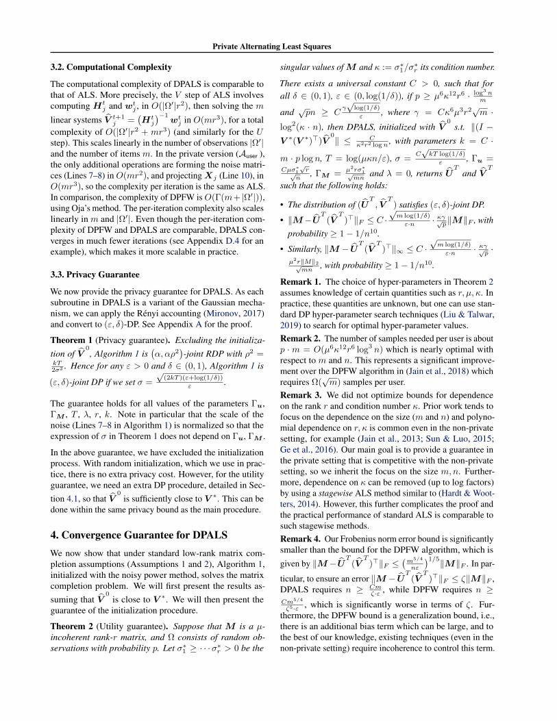
The first heuristics are motivated by the observation that,in practice, the elements of Ω are not sampled uniformlyat random (Marlin et al., 2007). In particular, the numberof observed ratings per item typically follows a power-lawdistribution, and is heavily skewed towards popular items.For example, Figure 2 shows the fraction of observations vs.fraction of top movies in the MovieLens 10M data set. Itshows, for instance, that the top 20% of the movies accountfor more than 85% of the observations.
Private Alternating Least Squares
0.0 0.2 0.4 0.6 0.8 1.0Movie fraction
0.0
0.2
0.4
0.6
0.8
1.0
Data
frac
tion
ML10M (unsampled)Uniform sampling (k = 50)Adaptive sampling (k = 50)
Figure 2. Fraction of observations contributed by the top moviesin MovieLens 10M. Adaptive sampling reduces popularity bias.
Due to this popularity bias, some items may have very fewobservations, and for such rare items j, the embedding V j
learned by DPALS may not be useful: The noise terms inLine 10 of Algorithm 1 do not scale with the number of ob-servations |Ω′j | – for otherwise we may lose the protectionon users who rated rare items – thus, items with a smaller|Ω′j | have a lower signal-to-noise ratio. In our experiments,we found that such noisy embeddings may have a furthercascading effect and lead to quality degradation in the em-beddings of other movies and users. To alleviate this issue,we propose two techniques.
Learning on frequent items. The first strategy is to par-tition the items into two sets, based on an estimate of theitem counts, which we denote by c ∈ Rn. We introduce ahyper-parameter β representing the fraction of movies totrain on. Define the set Frequent to be the dmβe items withthe largest c, and let Infrequent be its complement. Welearn embeddings V j only for j ∈ Frequent , by runningAlgorithm ADPALS on those items. When making predic-tions for any missing entry M ij , if j ∈ Frequent , we usethe dot product U i · V j , and if j ∈ Infrequent we use theaverage observed rating of PΩ(M)i.
To compute c privately, notice that since each user con-tributes at most k items, the exact item count c has `2sensitivity
√k. Thus, c := c + N (0, kσ2) guarantees(
α, α/2σ2)-RDP.
Adaptive sampling. To further reduce the popularitybias, we propose to use an adaptive distribution when sub-sampling Ω. Recall that in Line 6 of Aitem , we pick k itemsper user in Ω, in order to limit the privacy loss. We proposeto sample rare items with higher probability, as follows.Given the count estimate c, for each user i, we pick the kitems in Ωi∩Frequent with the lowest count estimates. Thisheuristic effectively reduces the distribution skew and givesa significant utility gain compared to uniform sampling, seeSection 6.3. Figure 2 illustrates the resulting distributionfor a sample size of k = 50 per user. It’s interesting toobserve that under uniform sampling, the popularity biasis worse than in the unsampled data set, this is due to anegative correlation between user counts and item counts:
conditioned on a light user, the probability to observe a rareitem is lower; see Appendix C for further discussion.
5.2. Additional Heuristics
A common heuristic, used for example by (McSherry &Mironov, 2009), is to center the observed matrix PΩ(M),by subtracting an estimate of the global average, denotedby m. To compute m privately, since ‖PΩ(M)‖∞ ≤ ΓM
and each user contributes at most k items, publishing m =∑(i,j)∈Ω Mij+N (0,kΓ2
Mσ2)
|Ω|+N (0,kσ2) guarantees(α, α/σ2
)-RDP.
Another practice, commonly used in some benchmarks, isto modify the loss function in Section 2.2 by adding theterm λ0‖U V >‖2F , where λ0 is a hyper-parameter. Thisis particularly important for item recommendation tasks,such as the MovieLens 20M benchmark. This modificationintroduces an additional term K := λ0
∑i∈[n] U i ⊗ U i to
X in Line 9 of Aitem . To maintain privacy, we use a noisyversion K obtained by adding Gaussian noise to K. SinceK is independent of j, we reuse the same K for all j ∈ [m],thus limiting the additional privacy loss due to this term.
Finally, we project the matrix Xj = Hj + Gj to the PSDcone (Line 9) to improve stability. In our analysis, we showthat Xj is positive definite with high probability, but inpractice, the projection improves performance.
We account for the privacy cost in the computation of m, c,and K, along with that in Theorem 1, by standard composi-tion properties of RDP (Mironov, 2017). For completeness,the privacy accounting of the full algorithm including datapre-processing, is given in Appendix C.
6. Empirical EvaluationWe run experiments on synthetic data and two benchmarktasks on the widely used MovieLens data sets (Harper &Konstan, 2016). The synthetic task follows the assumptionsof our theoretical analysis, and serves to illustrate the guaran-tees of Theorem 2. The MovieLens benchmark tasks serveas an evaluation of the empirical privacy/utility trade-off ona more realistic application, and to provide some practicalinsights into DPALS. We use current SOTA method DPFWas the main baseline as it is already demonstrated to bemore accurate than techniques like Private SVD (McSherry& Mironov, 2009). Similar to (Jain et al., 2018), we donot compare against (Liu & Talwar, 2019) as the privacyparameters are unclear, and might require (exponential time)Markov chain based sampling methods to compute them.
6.1. Metrics and Data Sets
Metrics. The quality of a learned model (U , V ) will bemeasured either using the RMSE or the Recall@k, de-

Private Alternating Least Squares
1 4 8 12 16ε
0.75
0.80
0.85
0.90
0.95
1.00
1.05
1.10te
st e
rror (
RMSE
)
1 5 10 15 20ε
0.75
0.80
0.85
0.90
0.95
1.00
1.05
1.10
test
erro
r (RM
SE)
1 5 10 15 20ε
0.15
0.20
0.25
0.30
0.35
test
qua
lity
(Rec
all@
20)
DPSVD Simple baseline DPFW DPALS ALS
(a) ML-10M (top 400 movies) (b) ML-10M (c) ML-20M
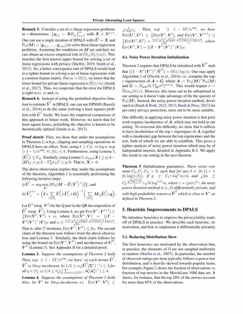
Figure 3. Privacy/utility trade-off of different methods. We observe that DPALS is significantly more accurate than DPFW method, andthe loss in accuracy for DPALS compared to ALS is relatively small, especially for ε ≥ 10.
1 5 10 15 20ε
10−2
10−1
100
test
erro
r (RM
SE)
DPFW, n=5KDPFW, n=10KDPFW, n=20KDPFW, n=50KDPALS, n=5KDPALS, n=10KDPALS, n=20KDPALS, n=50K
Figure 4. Comparison of DPFW and DPALS on synthetic data withdifferent number of rows/users n.
pending on the benchmark. The RMSE is defined asRMSE = ‖PΩtest(U V > −M)‖F /
√|Ωtest|, where Ωtest is
the set of test ratings held out from Ω. Recall@k is definedas follows. For each user i, letRi be the set of k movies withthe highest scores, where the score of movie j is U i · V j .Then Recall@k = 1
n
∑ni=1 |Ri ∩ Ωtest
i |/min(k, |Ωtesti |).
Synthetic data. We generate a rank 5 ground truth ma-trix as the product of two random orthogonal matricesU∗ ∈ Rn×5,V ∗ ∈ Rm×5, where m = 1000, andn ∈ 5000, 10000, 20000, 50000. We scaled the groundtruth matrix such that the standard deviation of the obser-vations is 1, in other words, a trivial model which alwayspredicts the global average has a RMSE of 1. The observedentries Ω are obtained by sampling each entry independentlywith probability p = 20 log(n)/m.
MovieLens data sets. We apply our method to two com-mon recommender benchmarks: (i) rating prediction onMovieLens 10M (ML-10M) following Lee et al. (2013),where the task is to predict the value of a user’s rating, andperformance is measured using the RMSE, (ii) item recom-mendation on MovieLens 20M (ML-20M) following Lianget al. (2018), where the task is to select k movies for eachuser and performance is measured using Recall@k. Forcomparison to DPFW, we use a variant of the ML-10M taskfollowing Jain et al. (2018), where the movies are restricted
to the 400 most popular movies (DPFW did not scale to thefull data set with all movies, unlike DPALS).
Experimental protocol. Each data set is partitioned intotraining, validation and test sets. Hyper-parameters arechosen on the validation set, and the final performance ismeasured on the test set. The privacy loss accounting isdone using RDP, then translated to (ε, δ)-DP with δ = 10−5
for the synthetic data and ML-10M and δ = 1/n for ML-20M. When training DPALS models on synthetic data, weuse the basic Algorithm 1, without heuristics. When train-ing on MovieLens, we use the heuristics described in Sec-tion 5. Note that even when training on Frequent items(Section 5.1), evaluation is always done on the full set ofitems, so that the reported metrics are comparable to pre-viously published numbers. Additional details on the ex-perimental setup are in Appendix D, including a list ofhyper-parameters and the ranges we used for each.
6.2. Privacy-Utility Trade-Off
DPALS vs. DPFW on synthetic data. On synthetic data(Figure 4) we observe: First, as expected, the trade-off ofboth algorithms improves as the number of users increases.Second, for ε = 1, the quality of the DPFW models isno better than the trivial model (RMSE equal to 1), whileDPALS has a lower RMSE, which significantly improveswith larger n. Third, for the largest data set (n = 50K), therelative improvement in RMSE between DPALS and DPFWis at least 7-fold across all values of ε. To further illustratethe difference between DPALS and DPFW, we show inAppendix D.4 the RMSE against number of iterations, bothfor the private and non-private variants (Figure 7).
DPALS vs. DPFW on ML10M. Next, we compare the twomethods on ML-10M-top400 (Figure 3a). For DPFW andDPSVD, the numbers are taken directly from (Jain et al.,2018). For reference, we include the test RMSE of non-private ALS, and a simple baseline model that always pre-

Private Alternating Least Squares
dicts the global average rating. The performance of DPSVDis worse than that of the simple baseline. DPALS performsbest, with a relative improvement in RMSE (compared toDPFW) that ranges from 7% to 11.6%, and that increaseswith ε. In Appendix D.4, we show that DPALS achieves per-formance better than DPFW even when trained on a smallfraction of the users (23%).
Finally, Figure 3b shows the privacy/utility trade-off onthe full ML-10M data. In order to scale DPFW to thethe full data, we use the same procedure described in Sec-tion 5: DPFW is trained on the top movies, and for remain-ing movies the model predicts the user’s average rating.Compared to the restricted data set (ML-10M-top400), theprivacy-utility trade-off is worse on the full data. This in-dicates that a smaller ratio between number of users andnumber of items makes the task harder – a result that is inline with the theory.
The results on synthetic data and ML10M suggest thatDPALS exhibits a much better privacy/utility trade-off thanDPFW, and a better dependence on the number of rows n,which is consistent with the theoretical analysis.
DPALS on MovieLens 20M. Figure 3c shows the pri-vacy/utility trade-off of DPALS on the ML-20M data set.We include as a reference the non-private ALS, and a simplebaseline model that always returns the k most rated movies.
On this task, the performance of the private model is re-markably good. Indeed, the best previously reported Re-call@20 numbers for non-private models on this benchmarkare 36.0% for ALS (Liang et al., 2018) and 41.4% usinga sophisticated auto-encoder model (Shenbin et al., 2020).Our results show that DPALS can achieve performance com-parable to the previously reported state of the art numbersfor (non-private) matrix completion, and the utility does notsignificantly degrade, even at small ε.
6.3. Importance of Adaptive Sampling and Projection
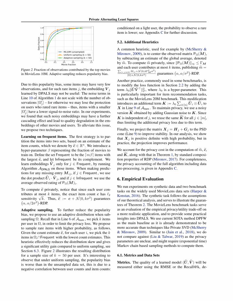
In this section, we give additional insights into the effect ofthe heuristics introduced in Section 5. We run a study onML-10M for ε = 10, r = 128 and a sample size k = 50(both correspond to the best overall model); other hyper-parameters are re-tuned. According to Section 5.1, we par-tition the set of movies into Frequent and Infrequent andtrain only on Frequent . The results are reported in Fig-ure 5, where the movie fraction is simply |Frequent |/n. Wemake the following observations. First, for non-private ALS,we get the highest RMSE by training on all movies, whilethere is a benefit for training on a subset of the movies forthe private models. Second, when training the non-privatemodel on sub-sampled data (red and purple lines), there is aconsiderable increase in RMSE, from 0.785 to 0.812. Thisgives an indication that part of the utility loss is due to sub-
0.0 0.2 0.4 0.6 0.8 1.0Movie fraction
0.75
0.80
0.85
0.90
0.95
1.00
1.05
test
erro
r (RM
SE)
DPALS, no projectionDPALS, uniformDPALS, adaptiveALS, uniformALS, adaptiveALS
Figure 5. RMSE vs. movie fraction for ε = 10 on ML-10M.
sampling, and not simply due to the addition of noise. Third,the sampling strategy has a significant impact on the per-formance of the private DPALS model: adaptive samplingimproves the RMSE from 0.870 to 0.854, in contrast, thesampling strategy appears to have little effect on non-privatemodels (i.e. models trained without noise). Finally, trainingthe private model without PSD projection (ΠPSD in Line 10of Algorithm 1) results in a terrible performance. We findthat while the projection is not technically necessary for thetheoretical analysis, it is essential in practice.
Training on a subset of the movies appears to have onlya marginal effect when combined with adaptive sampling.However, as detailed in the appendix, the effect is muchmore significant for smaller ε, as well as on ML-20M.
Additional experiments are presented in Appendix D, toexplore the effect of other hyper-parameters, such as therank and the regularization of the objective function.
7. ConclusionWe presented DPALS for solving low-rank matrix com-pletion with user-level privacy protection. We show thatDPALS provably converges to high accuracy outputs understandard assumptions and, with careful implementation, sig-nificantly outperforms existing privacy preserving matrixcompletion methods. In fact, DPALS achieves competitivemetrics on benchmark data compared to non-private modelsand scales well with data set size.
The efficiency of DPALS shows that by taking advantage ofthe structure of the problem, one can achieve a much higherutility for privacy-preserving model training. In this case,the alternating structure of ALS, along with the decouplingof the least squares solution, were essential in the design ofan efficient method. These insights may be applicable to abroader class of problems and optimization algorithms.
AcknowledgmentsWe would like to thank Om Thakkar and the anonymousreviewers for insightful comments and discussion.

Private Alternating Least Squares
ReferencesAbadi, M., Chu, A., Goodfellow, I., McMahan, H. B.,
Mironov, I., Talwar, K., and Zhang, L. Deep learningwith differential privacy. In Proceedings of the 2016 ACMSIGSAC conference on computer and communicationssecurity, pp. 308–318, 2016.
Bassily, R., Smith, A., and Thakurta, A. Private empiricalrisk minimization: Efficient algorithms and tight errorbounds. In Proc. of the 2014 IEEE 55th Annual Symp. onFoundations of Computer Science (FOCS), 2014.
Bhatia, R. Matrix analysis, volume 169. Springer Science& Business Media, 2013.
Calandrino, J. A., Kilzer, A., Narayanan, A., Felten, E. W.,and Shmatikov, V. “you might also like:” privacy risksof collaborative filtering. In 2011 IEEE symposium onsecurity and privacy, pp. 231–246. IEEE, 2011.
Candes, E. J. and Recht, B. Exact matrix completion via con-vex optimization. Foundations of Computational mathe-matics, 9(6):717–772, 2009.
Carlini, N., Liu, C., Erlingsson, U., Kos, J., and Song,D. The secret sharer: Evaluating and testing unintendedmemorization in neural networks. In 28th USENIX Se-curity Symposium (USENIX Security 19), pp. 267–284,2019.
Carlini, N., Deng, S., Garg, S., Jha, S., Mahloujifar, S.,Mahmoody, M., Song, S., Thakurta, A., and Tramer, F.An attack on instahide: Is private learning possible withinstance encoding? arXiv preprint arXiv:2011.05315,2020a.
Carlini, N., Tramer, F., Wallace, E., Jagielski, M., Herbert-Voss, A., Lee, K., Roberts, A., Brown, T., Song, D., Er-lingsson, U., et al. Extracting training data from large lan-guage models. arXiv preprint arXiv:2012.07805, 2020b.
Dekel, Y., Lee, J. R., and Linial, N. Eigenvectors of randomgraphs: Nodal domains. Random Structures & Algo-rithms, 39(1):39–58, 2011.
Dinur, I. and Nissim, K. Revealing information while pre-serving privacy. In Proceedings of the twenty-secondACM SIGMOD-SIGACT-SIGART symposium on Princi-ples of database systems, pp. 202–210, 2003.
Dwork, C. and Roth, A. The algorithmic foundations of dif-ferential privacy. Foundations and Trends in TheoreticalComputer Science, 9(3–4):211–407, 2014.
Dwork, C., Kenthapadi, K., McSherry, F., Mironov, I.,and Naor, M. Our data, ourselves: Privacy via dis-tributed noise generation. In Advances in Cryptology—EUROCRYPT, pp. 486–503, 2006a.
Dwork, C., McSherry, F., Nissim, K., and Smith, A. Calibrat-ing noise to sensitivity in private data analysis. In Proc.of the Third Conf. on Theory of Cryptography (TCC), pp.265–284, 2006b.
Dwork, C., McSherry, F., and Talwar, K. The price ofprivacy and the limits of lp decoding. In Proceedings ofthe thirty-ninth annual ACM Symposium on Theory ofComputing, pp. 85–94, 2007.
Dwork, C., Talwar, K., Thakurta, A., and Zhang, L. Analyzegauss: optimal bounds for privacy-preserving principalcomponent analysis. In Proceedings of the forty-sixthannual ACM symposium on Theory of computing, pp.11–20, 2014.
Erdos, L., Knowles, A., Yau, H.-T., and Yin, J. Spectralstatistics of erdos–renyi graphs i: Local semicircle law.The Annals of Probability, 41(3B):2279–2375, 2013.
Ge, R., Lee, J. D., and Ma, T. Matrix completion has nospurious local minimum. Advances in Neural InformationProcessing Systems, pp. 2981–2989, 2016.
Hardt, M. and Price, E. The noisy power method:A meta algorithm with applications. arXiv preprintarXiv:1311.2495, 2013.
Hardt, M. and Roth, A. Beating randomized response onincoherent matrices. In Proceedings of the forty-fourthannual ACM symposium on Theory of computing, pp.1255–1268, 2012.
Hardt, M. and Roth, A. Beyond worst-case analysis in pri-vate singular vector computation. In Proceedings of theforty-fifth annual ACM symposium on Theory of comput-ing, pp. 331–340, 2013.
Hardt, M. and Wootters, M. Fast matrix completion withoutthe condition number. In Conference on learning theory,pp. 638–678. PMLR, 2014.
Hardt, M., Meka, R., Raghavendra, P., and Weitz, B. Com-putational limits for matrix completion. In Conferenceon Learning Theory, pp. 703–725. PMLR, 2014.
Harper, F. M. and Konstan, J. A. The movielens datasets:History and context. Acm Transactions on InteractiveIntelligent Systems (TiiS), 5(4):19, 2016.
Hu, Y., Koren, Y., and Volinsky, C. Collaborative filteringfor implicit feedback datasets. In Proceedings of the 2008Eighth IEEE International Conference on Data Mining,ICDM ’08, pp. 263–272, 2008.
Jain, P. and Netrapalli, P. Fast exact matrix completion withfinite samples. In Conference on Learning Theory, pp.1007–1034. PMLR, 2015.
Private Alternating Least Squares
Jain, P., Netrapalli, P., and Sanghavi, S. Low-rank matrixcompletion using alternating minimization. In Proceed-ings of the forty-fifth annual ACM symposium on Theoryof computing, pp. 665–674, 2013.
Jain, P., Thakkar, O. D., and Thakurta, A. Differentiallyprivate matrix completion revisited. In International Con-ference on Machine Learning, pp. 2215–2224. PMLR,2018.
Kearns, M., Pai, M., Roth, A., and Ullman, J. Mechanismdesign in large games: Incentives and privacy. In Proceed-ings of the 5th conference on Innovations in theoreticalcomputer science, pp. 403–410, 2014.
Koren, Y. and Bell, R. Advances in collaborative filtering.Recommender systems handbook, pp. 77–118, 2015.
Koren, Y., Bell, R., and Volinsky, C. Matrix factorizationtechniques for recommender systems. Computer, 42(8):30–37, 2009.
Korolova, A. Privacy violations using microtargeted ads: Acase study. In 2010 IEEE International Conference onData Mining Workshops, pp. 474–482. IEEE, 2010.
Lee, J., Kim, S., Lebanon, G., and Singer, Y. Local low-rank matrix approximation. In Proceedings of the 30thInternational Conference on International Conference onMachine Learning - Volume 28, ICML’13, pp. II–82–II–90. JMLR.org, 2013.
Liang, D., Krishnan, R. G., Hoffman, M. D., and Jebara,T. Variational autoencoders for collaborative filtering.WWW ’18, pp. 689–698, 2018.
Liu, J. and Talwar, K. Private selection from private candi-dates. In Proceedings of the 51st Annual ACM SIGACTSymposium on Theory of Computing, pp. 298–309, 2019.
Liu, Z., Wang, Y.-X., and Smola, A. Fast differentiallyprivate matrix factorization. In Proceedings of the 9thACM Conference on Recommender Systems, pp. 171–178,2015.
Lu, S., Hong, M., and Wang, Z. PA-GD: On the convergenceof perturbed alternating gradient descent to second-orderstationary points for structured nonconvex optimization.In Proceedings of the 36th International Conference onMachine Learning, pp. 4134–4143, 2019.
Marlin, B. M., Zemel, R. S., Roweis, S., and Slaney, M. Col-laborative filtering and the missing at random assumption.In Proceedings of the Twenty-Third Conference on Un-certainty in Artificial Intelligence, UAI’07, pp. 267–275,Arlington, Virginia, USA, 2007. AUAI Press.
McSherry, F. and Mironov, I. Differentially private recom-mender systems: Building privacy into the netflix prizecontenders. In Proceedings of the 15th ACM SIGKDDinternational conference on Knowledge discovery anddata mining, pp. 627–636, 2009.
Meng, X., Wang, S., Shu, K., Li, J., Chen, B., Liu, H.,and Zhang, Y. Personalized privacy-preserving socialrecommendation. In Proceedings of the AAAI Conferenceon Artificial Intelligence, volume 32, 2018.
Mironov, I. Renyi differential privacy. In 2017 IEEE 30thComputer Security Foundations Symposium (CSF), pp.263–275. IEEE, 2017.
Recht, B. A simpler approach to matrix completion. Journalof Machine Learning Research, 12(12), 2011.
Rendle, S., Zhang, L., and Koren, Y. On the difficulty ofevaluating baselines: A study on recommender systems.CoRR, abs/1905.01395, 2019.
Rudelson, M. and Vershynin, R. Delocalization of eigenvec-tors of random matrices with independent entries. DukeMathematical Journal, 164(13):2507–2538, 2015.
Sheffet, O. Old techniques in differentially private linearregression. In Algorithmic Learning Theory, pp. 789–827.PMLR, 2019.
Shenbin, I., Alekseev, A., Tutubalina, E., Malykh, V., andNikolenko, S. I. Recvae: A new variational autoencoderfor top-n recommendations with implicit feedback. InProceedings of the 13th International Conference on WebSearch and Data Mining, WSDM ’20, pp. 528–536, 2020.
Shokri, R., Stronati, M., Song, C., and Shmatikov, V. Mem-bership inference attacks against machine learning mod-els. In 2017 IEEE Symposium on Security and Privacy(SP), pp. 3–18. IEEE, 2017.
Smith, A., Thakurta, A., and Upadhyay, J. Is interaction nec-essary for distributed private learning? In 2017 IEEE Sym-posium on Security and Privacy (SP), pp. 58–77. IEEE,2017.
Song, S., Chaudhuri, K., and Sarwate, A. D. Stochasticgradient descent with differentially private updates. In2013 IEEE Global Conference on Signal and InformationProcessing, pp. 245–248. IEEE, 2013.
Sun, R. and Luo, Z. Guaranteed matrix completion vianonconvex factorization. In FOCS, 2015.
Thakkar, O., Ramaswamy, S., Mathews, R., and Beaufays,F. Understanding unintended memorization in federatedlearning. arXiv preprint arXiv:2006.07490, 2020.
Private Alternating Least Squares
Tropp, J. A. An introduction to matrix concentration in-equalities. arXiv preprint arXiv:1501.01571, 2015.
Vershynin, R. Introduction to the non-asymptotic analysisof random matrices. arXiv preprint arXiv:1011.3027,2010.
Vu, V. and Wang, K. Random weighted projections, ran-dom quadratic forms and random eigenvectors. RandomStructures & Algorithms, 47(4):792–821, 2015.
Zhu, Y. and Wang, Y.-X. Improving sparse vector tech-nique with renyi differential privacy. Advances in NeuralInformation Processing Systems, 33, 2020.

Private Alternating Least Squares
A. Proof of Theorem 1Proof. To prove the guarantee for Algorithm 1, it suffices to show the following claim: that at each time step t ∈ [T ], thecomputations of X and
∑i∈Ω′j
M ij ·U i, for all j ∈ [m] satisfy(α, α k
2σ2
)-RDP. One can then compose the privacy losses
via simple Renyi composition (Mironov, 2017) to obtain the overall RDP-cost to be(α, α kT
2σ2
).
To prove the claim, notice that at each time step t ∈ [T ], there are m computations of X and∑i∈Ω′j
M ij ·U i. Since eachuser i ∈ [n] can affect only k of those computations, by Gaussian mechanism (Dwork et al., 2006a; Mironov, 2017) andthe generalization of standard composition property of RDP (Mironov, 2017, Proposition 1) to the joint RDP, we have therequired guarantee.
We now translate joint-RDP to join-DP. By the first part of the theorem, Algorithm 1 is (α, αρ2)-joint RDP with ρ2 = kT2σ2 .
Thus by (Mironov, 2017, Proposition 3) it is (ε, δ)-joint DP with ε = αρ2 + log(1/δ)α−1 for any α > 1. The latter expression is
minimized when α = 1+
√log(1/δ)
ρ , which yields εmin(ρ) = αρ2+ log(1/δ)α−1 = 2
√log(1/δ)ρ+ρ2. Now fix ε > 0, δ ∈ (0, 1).
To guarantee (ε, δ)-joint DP while minimizing the noise (which scales as 1/ρ by definition of ρ), it suffices to maximizeρ subject to εmin(ρ) ≤ ε, but since εmin is increasing in ρ, ρ is maximized when εmin(ρ) = ε. This is a second-orderpolynomial in ρ, and it has a positive root at ρ+ =
√log(1/δ) + ε−
√log(1/δ). Therefore, setting
σ =
√kT/2
ρ+=
√kT/2√
log(1/δ) + ε−√
log(1/δ)=
√kT/2(
√log(1/δ) + ε+
√log(1/δ))
ε≤√
2kT (log(1/δ) + ε)
ε
suffices to guarantee (ε, δ)-joint DP. This completes the proof.
B. Proofs from Section 4Recall the problem setting. M = U∗Σ∗(V ∗)> where (U∗)>U∗ = I and (V ∗)>V ∗ = I . Also, U∗ and V ∗ areµ-incoherent by assumption. That is, ‖U∗i ‖2 ≤ µ
√r/√n and ‖V ∗j‖2 ≤ µ
√r/√m. The set of observations is Ω =
(i, j) s.t. δij = 1, where δij are i.i.d. Bernoulli random variables with Pr[δij = 1] = p. We sample a new set ofobservations before every update.
We now present a basic lemma.
Lemma 6. Let U∗ and U t be µ and µ1-incoherent, orthonormal matrices where µ1 ≥ µ and n · p ≥ µµ1r2. Then, the
following holds for all j ∈ [m] (w.p. ≥ 1−mβ):∥∥∥∥∥1
p
n∑i=1
δijU∗i (U
ti)> − (U∗)>U t
∥∥∥∥∥F
≤ C
õ2
1r
n · p· log
r
β.
Proof. The proof follows from the matrix Bernstein inequality (Tropp, 2015, Theorem 6.1.1) and incoherence of U∗,U t.
Lemma 7. Let δij be i.i.d. Bernoulli random variables with Pr[δij = 1] = p. Then, the following holds (w.p. ≥ 1− δ):∥∥∥∥1
pPΩ(M)−M
∥∥∥∥F
≤ C(√
n
plog
1
β+
1
plog
1
β
)· ‖M‖∞.
Proof. The lemma is similar to Theorem 7 of (Recht, 2011) and follows by the matrix Bernstein inequality (Tropp, 2015,Theorem 6.1.1).
B.1. Rank-1 Case
Simplifying the notation, denote M = σ∗u∗(v∗)> where (u∗)>u∗ = 1 and (v∗)>v∗ = 1.
Note that as k = C · p ·m log n w.p. ≥ 1− T/n100, we do not throw any tuples in Line 6 of Algorithm 1. Similarly, usingincoherence we have: ‖M‖∞ ≤ ΓM . So, we do not clip any sample in Line 1 of Algorithm 1.

Private Alternating Least Squares
Now, we use mathematical induction to show the incoherence of resulting vt and ut, and to show that the clipping operationsdo not really apply in our setting with the selected hyper-parameters.
For the base case (t = 0), initialization of v0 ensures that Err(v∗,v0) ≤ Clogn . Now, using (Jain et al., 2013, Lemma C.2)
that uses clipping only in the first step to ensure incoherence, we get that v0 is 16µ-incoherent.
In the induction step, assuming the Lemma holds for vt, we prove the claim for ut and vt+1. Dropping superscripts of Ω′ifor notation simplicity and using λ = 0, we have: ut = arg min
u
∥∥PΩ
(M − u(vt)>
)∥∥2
F. The update of ut = ut/‖ut‖2.
So using (Jain et al., 2013, Lemma 5.5, Lemma 5.7, Theorem 5.1), we get w.p. ≥ 1− 1/n100:
ut is 16µ-incoherent,
‖ut‖2 ≥ σ∗/16,
Err(ut,u∗) ≤ 1
4Err(vt,v∗). (3)
To complete the claim, we only need to study the update for vt+1, which is a noisy version of the ALS update:
vt+1 = (D + Gt)−1(PΩ(M)ut + g
),
where D and Gt are diagonal matrices s.t. Djj =∑
(i,j)∈Ω(uti)2 and Gt
jj ∼ Γ2uσ · N (0, 1).
We first prove that D + Gt is indeed invertible, and has lower-bounded smallest eigenvalue. Using Lemma 6, andpn ≥ µ2 log n log(1/δ), we have w.p. ≥ 1−mδ,
1
pDjj ≥ ‖ut‖22
(1−
√1
log n
).
Also, using maximum of Gaussians, we have w.p. ≥ 1−mβ,
1
p
∥∥Gt∥∥
2≤
Γ2uσ√
log(n/β)
p≤µ2(σ∗)2σ
√log(n/β)
np≤ ‖ut‖22
16× 256,
where the final inequality follows by the assumption on p.
So,
‖(D + Gt)−1‖2 ≤2
p · ‖ut‖22. (4)
We now conduct error analysis for vt+1:vt+1 = α · v∗ −E,
where α = σ∗·(u∗)>ut
‖ut‖2. Furthermore, for a matrix C with Cjj =
∑(i,j)∈Ω utiu
∗i , we have E = E1 + E2 with
E1j = (Djj + Gt
jj)−1(αDjj − σ∗Cjj)v
∗j , E2
j = (Djj + Gtjj)−1(αGt
jjv∗j − gj).
This step follows from the observation that (PΩ(M)ut)j = σ∗Cjjv∗j . (We note that E is a vector but we use upper case to
be consistent with Section B.2.)
Note that E[αDjj − σ∗Cjj ] = 0. Furthermore, using incoherence of v∗,∥∥∥ut∥∥∥
2≥ σ∗/16, and the Bernstein’s inequality,
we have:‖E1‖2 ≤
1
64Err(ut,u∗). (5)
Now,
‖E2‖2 ≤2√
log n
p ·∥∥∥ut∥∥∥2
2
·(16Γ2
uσ + ΓMΓuσ√m)≤ Cµ4
√log n
np· σ. (6)

Private Alternating Least Squares
Using (5) and (6),∥∥∥vt+1
∥∥∥2≥ 3/4.
Thus, we get:
Err(v∗,vt+1) ≤ 1
32Err(u∗,ut+1) +
Cµ4√
log n
np· σ.
Similarly, by incoherence of v∗ and using bound on E1j and E2
j , we get:
‖vt+1‖∞ ≤ 3µ.
Therefore
vt+1 is 16µ-incoherent,
Err(vt+1,v∗) ≤ 1
32Err(ut,u∗) +
Cµ4√
log n
np· σ. (7)
So, the inductive hypothesis holds. Furthermore, we get Theorem 2, by combining the error terms of ut and vt+1.
B.2. Rank-r Case
B.2.1. PROOF OF LEMMA 3
Note that as k = C · p ·m log n, w.p. ≥ 1− T/n100, we do not throw any tuples in Line 6 of Algorithm 1. Similarly, usingincoherence we have: ‖M‖∞ ≤ ΓM . So, we do not clip any samples in Line 1 of Algorithm 1.
Now, we use mathematical induction to show the incoherence of resulting Vt
and Ut, and to show that the clipping
operations do not really apply in our setting with the selected hyperparamters.
For the base case (t = 0), initialization of V0
ensures that (V0)>V
0= I and Err(V ∗, V
0) ≤ C
κ2r2 logn . Now, using (Jain
et al., 2013, Lemma C.2) that uses clipping only in the first step to ensure incoherence, we get that V0
is 16µ√r-incoherent.
For the induction step, assuming the Lemma holds for Vt, we prove the claim for U
tand V
t+1. Dropping superscripts
of Ω′i for notation simplicity and using λ = 0, we have: Ut
= arg minU
∥∥PΩ
(M −U(V t)>
)∥∥2
F. That is, the update of
Ut
= U tRU , with U t being the Q part of QR-decomposition, is identical to the standard non-noisy ALS. So using (Jainet al., 2013, Lemma 5.5, Lemma 5.7, Theorem 5.1)1, we get w.p. ≥ 1− 1/n100,
U t is 16κµ-incoherent,
‖Σ∗R−1U ‖2 ≤ 16κ, i.e., ‖R−1
U ‖2 ≤∥∥(Σ∗)−1
∥∥2‖Σ∗R−1
U ‖2 ≤ 16‖(Σ∗)−1‖2κ,
Err(U t,U∗) ≤ 1
4Err(V t,V ∗). (8)
That is, now to complete the claim we only need to study the update for Vt+1
, which is a noisy version of the ALS update.
Now consider,
Xtj = (U
t)>
∑i:(i,j)∈Ω
eie>i
Ut
+ Gtj = p ·RU
(U t)>
1
p
∑i:(i,j)∈Ω
eie>i
U t + N tj
RU , (9)
where Gt is the noise added in Line 9 of Algorithm 1 at time step t, Dtj = (U t)>
(1p
∑i:(i,j)∈Ω eie
>i
)U t and N t
j =1pR−1U Gt
jR−1U . Note that using Gaussian eigenvalue bound (Vershynin, 2010) and Weyl’s inequality (Bhatia, 2013), we
have w.p. ≥ 1− 1/n100,
σmin(Dtj + N t
j) ≥
(1− C
√µ2κ2r
n · p· log n− 2Γ2
uσ√r
p · σmin(RU )2
)≥ 1
2, (10)
1Lemma 5.5 of (Jain et al., 2013) has a redundant√r term in incoherence claim
Private Alternating Least Squares
where the last inequality follows from: np ≥ Cµ2κ2r log2 n and n√p ≥ Cµ2κ6r
√r ·√m logn·(T log(1/δ))
ε .
Next, we argue that Xtj is PSD. Observe that
σmin(Xtj) ≥
1
2p · σmin(RU )2 ≥ C p · σmin(Σ∗)2
κ2> 0, (11)
where the last inequality follows from (8).
This shows that X used in update of Vt+1
is PSD, and hence the update for Vt+1
is given by:
RU (Vt+1
)>j (12)
=(Dj + N tj)−1(CjΣ
∗(V ∗)>j + gtj)
(13)
=(U t)>U∗Σ∗(V ∗)>j (14)
− (Dj + N tj)−1(Dj(U
t)>U∗ −Cj)Σ∗(V ∗)>j − (Dj + N t
j)−1(N t
j(Ut)>U∗Σ∗(V ∗)>j − gtj), (15)
where Dj = (U t)>(
1p
∑i:(i,j)∈Ω eie
>i
)U t, Cj = (U t)>
(1p
∑i:(i,j)∈Ω eie
>i
)U∗, and gtj = 1
pR−1U gtj .
That is,
Vt+1
RU = V ∗Σ∗(U∗)>U t −E>, Ej = E1j + E2
j ,
E1j = (Dj + N t
j)−1(Dj(U
t)>U∗ −Cj)Σ∗(V ∗)>j , E2
j = (Dj + N tj)−1(N t
j(Ut)>U∗Σ∗(V ∗)>j − gtj). (16)
Let Vt+1
= V t+1RV . Then,
V t+1RVRU = V ∗Σ∗(U∗)>U t −E>, Ej = E1j + E2
j ,
E1j = (Dj + N t
j)−1(Dj(U
t)>U∗ −Cj)Σ∗(V ∗)>j , E2
j = (Dj + N tj)−1(N t
j(Ut)>U∗Σ∗(V ∗)>j − gtj). (17)
Using the technique of (Jain et al., 2013, Lemma 5.6) and the bound on σmin(Dtj + N t
j) (see (10)), we get:∥∥(Σ∗)−1E1∥∥F≤ C
κErr(U t,U∗). (18)
Similarly, w.p. ≥ 1− 1/n100:
‖(Σ∗)−1E2‖F ≤2
σmin(Σ∗)·
(Γ2uσ
pσmin(RU )2
σmax(Σ∗)µ√r2m log n√
m+
ΓuΓMσ
pσmin(RU )·√mr log n
),
≤ Cσ√
log n
pn·(κ5 · µ3r2 + µ3r2κ3
)≤ Cκ5 · µ3r2
√log n
√pn
·√m log n · T
√log(1/δ)
ε. (19)
Let β = Cκ5·µ3r2√logn√pn
√m logn·T log(1/δ)
ε . Now,
σmin(RVRU ) ≥ σmin(Σ∗)(1− 2Err(U t,U∗)− κβ
)≥ σmin(Σ∗)
2, (20)
where the last inequality holds because:
√pn ≥ Cκ6µ3r2
√mT log n
√log(1/δ)
ε.
Using (17), we have:
maxj
∥∥(V t+1)>j∥∥
2≤ 2µκ
√r√
m+
4µκ√r√
m+
2µκrΓ2uσ√
mpσmin(RU )2+
2ΓuΓMσ√r
pσmin(Σ∗)σmin(RU )≤ 16µκ
√r√
m, (21)
where the last inequality follows from the assumption that√pn ≥ Cκ6µ3r2
√mT logn
√log(1/δ)
ε . This concludes the proof.

Private Alternating Least Squares
B.2.2. PROOF OF LEMMA 4
The proof for this key Lemma follows technique similar to the above proof. That is, using previous lemma, the clippingoperations do not have any effect, and hence we get noisy ALS updates. Now, using (18), (19), (20), and Lemma 8, we have:
Err(V ∗,V t+1) ≤ 1
4Err(U∗,U t) + 4κβ. (22)
This proves the lemma.
B.3. Proof of Theorem 2
Using Lemma 8, we have:
Err(V ∗,V t) ≤ 1
4+ Err(V ∗,V t+1) + α,
where α ≤ Cκ6·µ3r2√logn√pn
√m logn·T log 1/δ
ε . So, after T = log Err(V ∗,V 0)α iterations, Err(V ∗,V T ) ≤ 2α.
As UT
= arg minU ‖M − UT
(V T )>‖F , we have:
‖M − UT
(V T )>‖F ≤ ‖M −U∗Σ∗(V T )>‖F ≤ ‖M‖F ‖V ∗ − V T ‖2 ≤ 2α‖M‖F , (23)
where last inequality follows from the fact that ‖V ∗ − V T ‖2 ≤ 2Err(V ∗,V ).
This shows the second claim of the theorem. The third claim follows similarly while using incoherence of V T .
Lemma 8. Let U = U∗Σ∗W +E and U = UR−1 where Σ∗ is a diagonal matrix, W ∈ Rr×r, and R2 = U>U . Then,
assuming σmin(Σ∗)σmin(W ) > ‖Σ∗‖2‖E(Σ∗)−1‖2, the following holds:
‖(I −U∗(U∗)>)U‖2 ≤‖E · (Σ∗)−1‖2
σmin(Σ∗)‖Σ∗‖2 σmin(W )− ‖E(Σ∗)−1‖2
.
That is,
‖(I −U∗(U∗)>)U‖2 ≤κ‖E‖2
σmin(Σ∗)σmin(W )− κ‖E‖2.
Proof.
‖(I −U∗(U∗)>)U‖2 ≤ ‖E ·R−1‖2 ≤ ‖E(Σ∗)−1‖2‖Σ∗R−1‖2.
Furthermore, ‖Σ∗R−1‖ ≤ ‖Σ∗‖2‖R−1‖2. Now,
1
‖R−1‖2= σmin(R) ≥ σmin(Σ∗)σmin(W )− ‖Σ∗‖2‖E(Σ∗)−1‖2.
That is,
‖(I −U∗(U∗)>)U‖2 ≤‖E · (Σ∗)−1‖2
σmin(Σ∗)‖Σ∗‖2 σmin(W )− ‖E · (Σ∗)−1‖2
.
B.4. Noisy Power Iteration Initialization
In this section, we derive a tighter initialization routine through the noisy power iteration procedure. We will show that itonly requires n = O(m) and can succeed with high probability.
Prior work on noisy power iteration requires A = PΩ(M)>PΩ(M) to be incoherent (Hardt & Roth, 2012; 2013; Hardt &Price, 2013). But whether this is true under our sparsity condition is a difficult problem. For example, related bounds, first

Private Alternating Least Squares
conjectured in (Dekel et al., 2011), have only been shown to hold for constant p (Vu & Wang, 2015; Rudelson & Vershynin,2015) but still open for p = O(logcm/m) for constant c > 0, the range interesting to us. To overcome this difficulty, weshow that we actually do not need A to be fully incoherent. Instead, we just need A’s top-r eigenspaces to be incoherent,and the existence of a (moderate) gap between the top eigenspaces and the rest, both of which we are able to establish.Given these two conditions, we then add the proper amount of noise, with a magnitude in between the top-r eigenvalues andthe rest, such that i) it does not interfere with the “boosting” of the top-r eigenspace; and ii) it “randomizes” the remainingeigenvectors such that their incoherence is preserved through the power iteration.
For simplicity, we will present a detailed proof in the rank-1 case. Here, we say a vector w ∈ Rm is µ-incoherent if‖w‖∞ ≤
µ√m
.
Algorithm 2 Noisy power iteration.Required: PΩ(M) ∈ Rn×m, number of iterations: T , incoherence parameter: ν, s: threshold formaximum number of ratings per user, entry clipping parameter: ΓM .
1 w1 ← Random unit vector in m-dimensions.for 1 ≤ t ≤ T do
2 If wt is not ν-incoherent, then report failure and stop.3 Compute zt =
(PΩ(M)>PΩ(M)
)·wt, and z ← zt + gt, where gt ∼ N
(0, σ2 · I
).
4 Normalize zt to obtain wt+1.endreturn wT+1.
Theorem 9 (Privacy guarantee). Algorithm 2 satisfies (α, αρ2)-RDP, where ρ2 =Ts3Γ4
Mν2
2mσ2 .
The proof follows immediately from `2-sensitivity analysis and the RDP guarantee for Gaussian mechanism (Mironov,2017).
For the utility guarantee, consider the case where Ω is randomly sampled with probability p (so setting s ≈ mp is sufficient).Furthermore, since we are in the rank-1 case, we will assume M =
√mn · u⊗ v, where both u and v are µ-incoherent so
ΓM can be set as µ2. Below we assume µ,ΓM = O(1) for simplicity. Now we will show that we can set p = O(log3m/m)and n = O(m logm
√log(1/δ)/ε), with proper choices of ν, σ, such that ρ2 ≤ (ε+log(1/δ))/ε2, and the above procedure
returns a vector w such that |w ·v| > 0.6 with probability 1−o(1), which can be boosted to high probability by the standardmethod.
Theorem 10 (Utility guarantee). There exists constant C1, C2 > 0, such that for any δ ∈ (0, 1), ε ∈ (0, log(1/δ)), if
p ≥ C1 log3 mm and
√pn ≥ C2
√log(1/δ)
ε ·√m log5/2m, then we can choose settings of incoherence parameter ν, noise
standard deviation σ, and number of time steps T in Algorithm 2 s.t., w.p. 1− o(1), we have |wT+1 · v| > 0.6, where v isthe right singular vector of M , and ρ = ε
2√
log(1/δ), i.e. Algorithm 2 satisfies (ε, δ)-differential privacy. The probability
guarantee can be boosted to high probability 1−m−c for any c > 0 with the private selection algorithm (Liu & Talwar,2019; Zhu & Wang, 2020).
Proof. We will prove this theorem through a sequence of claims. Write λ = p2mn. The following claim is from previouswork, e.g. (Recht, 2011).
Claim 11. For n = Ω(m), p = Ω( logmm ), with high probability, A = λ(v⊗v)+B, where ‖B‖2 = O(np
√logm). Hence,
if λ1,h1 are the principal eigenvalue and eigenvector, respectively, of A, then λ1 = (1± o(1))λ and |h1 · v| = 1− o(1).
One key fact we need is that h1 is not only close to v, but also incoherent. The proof essentially follows the arguments in theproof of Theorem 2.16 in (Erdos et al., 2013). One difference in our case is that the entries in A are not independent becauseA = PΩ(M)>PΩ(M). This difficulty was overcome in (Jain & Netrapalli, 2015)(Lemma 6) by using the resamplingtechnique. Here we present a direct argument, which might be of independent interest.
Claim 12. For n = Ω(m), p = Ω( log2 mm ), with high probability, the principal eigenvector of A is C-incoherent for some
absolute constant C > 0.

Private Alternating Least Squares
Proof. We treat PΩ(M) as the adjacency matrix of a random bipartite graph and apply the techniques similar to (Erdoset al., 2013; Jain & Netrapalli, 2015). Recall h1 is the principal eigenvector of A with the eigenvalue λ1. Denote byN = PΩ(M)− p
√mn(u⊗ v). We will first show that when np logm, with high probability, there exists w, where
‖w‖∞ = O(1/√m), such that
h1 = (1± o(1))
(I− 1
λ1N>N
)−1
w . (24)
Since λ1 = (1± o(1))λ,∥∥∥N>N∥∥∥
2= o(λ1), we can expand the above equation to:
h1 = (1± o(1))∑k≥0
(1
λ1N>N
)kw .
We then apply the method in (Erdos et al., 2013; Jain & Netrapalli, 2015) to show that there exists constant c0 < 1 such thatwith high probability: ∥∥∥∥∥
(1
λ1N>N
)kw
∥∥∥∥∥∞
≤ ck0‖w‖∞ . (25)
These would imply that h1 is O(1)-incoherent. We first prove (24). Since N = PΩ(M)− p√mn(u⊗ v), we can write
A = PΩ(M)>PΩ(M) = N>N + p√mn(v ⊗ u)PΩ(M) + p
√mnPΩ(M)>(u⊗ v)− p2mn(v ⊗ v) .
We first observe that with high probability v = 1p√mn
PΩ(M)>u satisfies that
|vj − vj | = O
(√logm
pn|vj |
)for all j ∈ [m]. (26)
Since |h1 · v| = 1− o(1), we have that when pn logm, |h1 · vj − h1 · v| = o(1). Hence
p√mn(v ⊗ u)PΩ(M)h1 = p
√mn(PΩ(M)>u · h1)v = p2mn((h1 · v)± o(1))v . (27)
In addition,p√mnPΩ(M)>(u⊗ v)h1 = p2mn(h1 · v)v . (28)
Applying (27) and (28), we have that
Ah1
=(N>N + p√mn(v ⊗ u)PΩ(M) + p
√mnPΩ(M)>(u⊗ v)− p2mn(v ⊗ v))h1
=N>Nh1 + p2mn((h1 · v)± o(1))v + p2mn(h1 · v)v − p2mn(h1 · v)v
=N>Nh1 + λ(h1 · v)(v ± o(1)v) .
Let w = (h1 ·v)(v±o(1)v). Recall ‖v‖∞ = O(1/√m). When pn logm, using (26), we have ‖v‖∞ = O(1/
√m) too.
Hence ‖w‖∞ = O(1/√m). Since Ah1 = λ1h1, we have that N>Nh1 + λw = λ1h1, hence (λ1I−N>N)h1 = λw,
which implies (24).
Now we prove (25). Since we λ1 = (1± o(1))λ, it suffices to prove (25) by replacing λ1 with λ instead. Furthermore, since
‖N>N‖2 = o(λ), it suffices to consider k = O(logm). Let N ′ = 1p√mn
N . Writew′ =(
1λN
>N)k
w = (N ′>N ′)kw.Following the proof of Lemma 7.10 in (Erdos et al., 2013), we will bound the q-th moment of |w′j | and apply the Markovinequality. We treat N ′ as the adjacency matrix of a bipartite graph [n]× [m] where each edge is labeled with a random
Private Alternating Least Squares
variable ξij = ( 1pχij − 1)uivj where χij’s are independent Bernoulli random variables taking value 1 with probability p.
By its definition E[ξij ] = 0, and for r ≥ 2,
E[|ξij |r] = p((1
p− 1)|uivj |)r + (1− p)(|uivj |)r = O
(p
1
(p√mn)r
). (29)
Let G = [n]× [m] denote the complete bipartite graph with each edge ij labeled with ξij . For j1, j2 ∈ [m], let Pk(j1, j2)denote all the length 2k paths in G starting from the node j1 and ending at node j2. Then,
w′j =∑j1
wj1∑
P∈Pk(j1,j)
∏e∈P
ξe .
Andw′j
q=
∑j1,j2,··· ,jq
wj1wj2 · · ·wjq∑
∀` P`∈Pk(j`,j)
∏e∈∪P`
ξe .
Here ∪`P` is understood as a multiple set. Hence
E[w′jq] =
∑j1,j2,··· ,jq
wj1wj2 · · ·wjq∑
∀` P`∈Pk(j`,j)
E[∏
e∈∪`P`
ξe]
≤ ‖w‖q∞∑
j1,j2,··· ,jq
∑∀` P`∈Pk(j`,j)
|E[∏
e∈∪`P`
ξe]| .
We will now bound ∑j1,j2,··· ,jq
∑∀` P`∈Pk(j`,j)
|E[∏
e∈∪`P`
ξe]| . (30)
Since E[ξij ] = 0 and ξij’s are independent random variables, for E[∏e∈∪`P`
ξe] 6= 0, it must be that every edge in ∪`P`appears at least twice. The bound on E[|w′j |q] is by counting the number of such paths and applying the moments bound(29).
The argument follows (Erdos et al., 2013). We give it here for completeness. Let P denote the set of edges, withoutmultiplicity, in ∪`P`. Write t = |P |. Then t ≤ kq since every edge in ∪`P` has to appear at least twice. In addition, theedges in P form a connected component because all the paths are connected to node j. Hence there are at most t+ 1 vertices.Since the set must include j, there are at most
(m+nt
)choices of the set of vertices. Among t+ 1 vertices, we can make at
most(t+2k
2k
)(2k)! different paths of length 2k. Hence the total number of paths is bounded by(
m+ n
t
)((t+ 2k
2k
)(2k)!
)q≤ nt(c1kq)2kq ,
for some c1 > 0. In the last inequality, we used that n = Ω(m) and t ≤ kq.
Suppose that P = e1, e2, · · · , et, and the multiplicity of these edges in ∪`P` are s1, s2, · · · , st respectively. So∑i si = 2kq. Using (29),
E
[ ∏e∈∪`P`
|ξe|
]= E[|ξe1 |s1 ] E[|ξe2 |s2 ] · · ·E[|ξet |st ]
=
(p
1
(p√mn)s1
)· · ·(p
1
(p√mn)st
)= pt
1
(p√mn)2kq
.
Hence the contribution to (30) by the case of |P | = t is bounded by:
nt(c1kq)2kqpt
1
(p√mn)2kq
=(c1kq)
2kq
(pm)kq(pn)kq−t.

Private Alternating Least Squares
Since t ≤ kq, (30) is bounded by
O
((c1kq)
2kq
(pm)kq
).
Fix c0 = 1/2. For any c > 0 and k = O(logm), we can choose q = logm/(2k) and p ≥ c′ log2m/m for some c′ > 0 suchthat (30) is bounded by ckq0 m−c. Applying Markov inequality, we have that with probability 1−m−c, |w′j | = O(ck0‖w‖∞).Since c can be chosen arbitrarily, we have that with high probability this holds for all k = O(logm). This completes theproof.
The following summarizes the above claims and the conditions we need in our proof.
Claim 13. Assume n = Ω(m), p = Ω( log3 mm ). Let A =
∑i
λi(hi ⊗ hi) be the eigen-decomposition of A where
λ1 ≥ λ2 ≥ . . . λm ≥ 0. Then λ1 = (1 ± o(1))p2mn, and for i ≥ 2, λi = O(np√
logm) = o(λ1/ log2m). In additionh1 · v = 1− o(1), and ‖h1‖∞ ≤ C/
√m.
Now we show that
Claim 14. There exists c2, c3 > 0, such that if σ ≥ c2 λ√m log3/2 m
, then ∀t ∈ [T ], wt’s are c3√
logm-incoherent.
Proof. For notation convenience, we set w0 = 0, hence w1 is a random unit vector. Write wt =∑i αtihi. Then
Awt =∑i λiαtihi and zt = Awt + gt =
∑i(λiαti + gti)hi, where gti = gt · hi. Hence α(t+1)i = (λiαti + gti)/‖zt‖2.
Since gt is sampled fromN (0, σ2I), gti’s are i.i.d Gaussian fromN (0, σ2). In addition α0i = 0. By induction, we have thatE[αti] = 0, and the signs sign(αt1), · · · , sign(αtm) are uniformly distributed in −1, 1m, independent of their values, bythe same argument in (Hardt & Price, 2013) Lemma 4.13. We will now first show, by induction, that with high probability,maxi≥2 |λiαti| = O(σ).
When t = 0, this is clearly true. Now suppose this holds for wt. All the following statements hold with high probability.Note in the following αti’s are random variables. By ‖zt‖2 =
∑i(λiαti + gti)
2 and maxi≥2 |λiαti| = O(σ) with highprobability, we have that with high probability,
‖zt‖22 = Ω(λ21α
2t1 +mσ2) . (31)
By induction hypothesis for any i ≥ 2, |λiαti| = O(σ), hence |λiαti + gti| = O(√
logmσ). Since ‖zt‖ = Ω(√mσ),
|α(t+1),i| = |λiαti + gti|/‖zt‖ = O(√
logm√m
), hence |λiα(t+1),i| = O( λlog2 m
·√
logm√m
) = O( λlog3/2 m
√m
) = O(σ). Wecan clearly choose c3 large enough to make sure the induction goes through.
The j-th coordinate of zt is zt(j) =∑i(λiαti + gti)hi(j). Consider zt(j)′ =
∑i≥2(λiαti + gti)hi(j). Clearly gti’s are
independent Gaussian variables. In addition, sign(αt1), · · · , sign(αtm) are uniformly distributed over −1, 1m. Since|λiαti| = O(σ) for i ≥ 2, and
∑i hi(j)
2 ≤ 1, by applying the concentration bound, we have that with high probability
|zt(j)′| = O(√
logm∑i≥2 σ
2hi(j)2)
= O(σ√
logm) .
Hence, with high probability,
zt(j)2 = O(λ2
1α2t1h1(j)2 + (logm)σ2) = O(λ2
1α2t1/m+ (logm)σ2) . (32)
The last inequality is by ‖h1‖∞ ≤ C/√m. Combining with Equation (31), by distinguishing the cases of |λ1αt1| ≤
√mσ
and |λ1αt1| ≥√mσ, we have that |zt(j)|
‖z‖2 = O(√
logm√m
), i.e wt is O(√
logm)-incoherent.
Now, we show that we need only O(logm) round to get a constant approximation to v. Note that here we cannot get highprobability bound because we need the initial |α01| to be Ω(1/
√m logm) to bootstrap the process. But it does happen with
probability 1− o(1).

Private Alternating Least Squares
Claim 15. There exists c4, c5 > 0, such that with n, p, σ, ν as set above, if T ≥ c4 logm, |wT · v| ≥ 1 − c5/ logm w.p.1− o(1).
Proof. It suffices to show that |αT1| = Ω(1). Because λ2 = O(λ1/ log2m) and√m logmσ = O(λ1/ logm), once
|αT1| = Ω(1), with one more round we would have |αT+1,1| = 1−O(1/ logm).
Suppose that |α01| = Ω(1/√m logm), which happens with probability 1 − o(1). Then |λ1α01| = Ω(logm)σ. We
can prove by induction that |λ1αt1| = Ω(logm)σ with high probability. By α(t+1)1 = (λ1αt1 + gt1)/‖zt‖2, we have|α(t+1)1| ≥ 1
2 |λ1αt1|/‖zt‖2 with high probability. By Equation (32), we can bound
‖zt‖22 = O(λ2
1α2t1 + (m logm)σ2
).
Hence,
|α(t+1)1| ≥1
2|λ1αt1|/‖zt‖2 = Ω(|λ1αt1|/(|λ1αt1|+
√m logmσ)) . (33)
Now if |λ1αt1| ≥√m logm · σ, then |α(t+1)1| = Ω(1) so we are done. Otherwise, |α(t+1)1| = Ω(|λ1αt1|/(
√m logm ·
σ)) = Ω(logm)|αt1|, by σ = O(
λ√m log3/2 m
). Hence within O(logm) rounds, αt1 ≥ c for some constant c > 0.
Now, gather the assumption ΓM = µ2 = O(1) and the conditions ν = O(√
logm), σ = Ω( p2mn√m log3/2 m
), T = O(logm)
and plug them into the formula in Theorem 9. We have that
ρ2 =T (mp)3Γ4
Mν2
2mσ2= O
(m log5m
pn2
). (34)
Hence we can set n = O
(√log(1/δ)
ε
√m/p log5/2m
), such that ρ2 = ε2
4 log(1/δ) . This completes the proof. We note that
when p = O(log3m/m), n = O(m logm) which is nearly optimal.
Note that the only reason that prevents the high probability guarantee is due to the choice of the initial random vector. It canbe boosted to high probability guarantee by running the process O(logm) times and privately releasing the vector w with‖PΩ(M)w‖2 above a threshold. This can be done through the private selection algorithm (Liu & Talwar, 2019) with anextra constant factor in ε.

Private Alternating Least Squares
C. Additional Details on Heuristic ImprovementsAlgorithm 3 summarizes the data pre-processing and sampling heuristics described in Section 5.
Algorithm 3 Data pre-processing heuristics.Required: PΩ(M): Observed ratings, ΓM : entry clipping parameter, k: maximumnumber of ratings per user, σp: standard deviation of the pre-processing noise, β:fraction of movies to train on.
1 Clip entries in PΩ(M) so that ‖PΩ(M)‖∞ ≤ ΓM
2 Uniformly sample Ω′:for 1 ≤ i ≤ n do
Ω′i ← sample k items from Ωi uniformly.end
3 Compute movie counts c← Counts(Ω′).4 Partition movies:
Let Frequent be the dβme movies with the largest c, and let Infrequent be the rest.5 Adaptively sample Ω′′:
for 1 ≤ i ≤ n doΩ′′i ← the k items in (Ωi ∩ Frequent ) with the lowest count c.
end6 Recompute movie counts c← Counts(Ω′′)
7 Center the data PΩ′′(M)← PΩ′′(M)− m, where m =∑
(i,j)∈Ω′′ Mij+N (0,kΓ2Mσ2
p)
|Ω′′|+N (0,kσ2p)
return PΩ′′(M), c
Procedure Counts(Ω)for 1 ≤ j ≤ m do
cj ← |Ωj |+N (0, σ2p)
return cend
First, we compute differentially private movie counts (Line 3) using a uniform sample Ω′, and use it to partition the movies(Line 4) and to perform adaptive sampling (Line 5). The final subset used for training is Ω′′, which consists only of Frequentmovies. Finally, to have a more accurate estimate of the counts, we recompute c on Ω′′ (Line 6). We redo this computationas the counts are also used during optimization, as described in the next section. Note that in both computations of c, we usea subset of Ω that contains at most k movies per user, in order to guarantee user-level differential privacy.
Privacy accounting. As we saw in Theorem 1, Algorithm 1 with random initialization satisfies(α, α(kT )
2σ2
)-joint RDP. The
data processing heuristics in Algorithm 3 satisfy(α, α(2k+2)
2σ2p
)-RDP. So, by standard composition of RDP, we have the
total privacy cost at any order α > 1 to be:(α, α ·
(kT2σ2 + k+1
σ2p
)). We can obtain the final (ε, δ)-joint differential privacy
guarantee by optimizing for α, similarly to Appendix A.
Loss function. We minimize the following loss in practice.
f(U , V ) = ‖PΩ
(M − U V >
)‖2F + λ0‖U V >‖2F + λ
n∑i=1
cνiZ‖U i‖2 + λ
m∑j=1
cµjZ ′‖V j‖2, (35)
where λ0, λ, µ, and ν are hyper-parameters. The loss function used in the description of Algorithm 1 is a special case of (35)where λ0 = µ = ν = 0. The additional terms in (35) do not change the essence of the algorithm, but we find that they makea significant difference in practice.
First, the term λ0‖U V >‖2F is often used in problems with implicit feedback, as in (Hu et al., 2008). In such problems, theobserved entries are often binary, and minimizing the objective ‖PΩ
(M − U V >
)‖2F can yield a trivial solution – the matrix
of all ones. The addition of the second term penalizes non-zero predictions outside of Ω, leading to better generalization.One of the benchmarks we use is an implicit feedback task, in which the use of the second term is necessary. As describedin Section 5.2, this results in an additional term K in Line 9 of Aitem , and care is needed when adding privacy protection to

Private Alternating Least Squares
this term, since it involves a sum over all user embeddings. The key observation is that this term is constant for all items, sowe only need to compute a noisy version of K once and use it for all items, thus limiting the privacy loss it incurs.
Second, we use a weighted `2 regularization, where the weights are defined as follows. The weight of movie j is cµj /Z′,
where c is the vector of approximate counts (computed in Algorithm 3), µ is a non-negative hyper-parameter and Z ′ is thenormalizing constant Z ′ = 1
m
∑mj=1 c
µj . When µ is positive, this corresponds to applying heavier regularization to more
frequent items, and we found in our experiments that this can significantly help generalization. The weights for the users aredefined similarly, with one main difference: instead of using approximate counts c, we use the exact counts c, as this termonly affects the solution in Auser , which is a privileged computation as illustrated in Figure 1.
102 103
User count101
102
103
104
Mov
ie c
ount
100
101
102
103
(a) ML-10M (unsampled)
102 103
User count101
102
103
104
Mov
ie c
ount
(b) Uniform sampling (k = 50)
102 103
User count101
102
103
104
Mov
ie c
ount
(c) Adaptive sampling (k = 50)
Figure 6. Histogram of user and movie counts in ML-10M, in the original data, and under uniform and adaptive sampling. The color barsin Figures 6b and 6c show the difference in marginal probability compared to the original data in 6a. Red indicates an increase in marginalprobability, while blue indicates a decrease. Note that the probability of frequent movies increases under uniform sampling, and decreasesunder adaptive sampling.
Effect of uniform and adaptive sampling. As observed in Figure 2, the movie count distribution of the MovieLens dataset is heavily skewed. We also observed that, perhaps surprisingly, uniformly sampling k items per user tangibly increasesthe skew. This can be explained by a negative correlation between user counts and movie counts; we computed a correlationcoefficient of −0.243. This is also visible in Figure 6a, which shows the joint histogram of (ci, cj), (i, j) ∈ Ω, whereci = |Ωi| is the user count (the number of ratings this user produced) and cj = |Ωj | is the movie count (the number ofratings the movie received). The figure illustrates that infrequent users are more likely to rate frequent movies than theaverage user. By uniformly sampling a constant number of movies per user (Figure 6b), we are, by definition, increasingthe probability of infrequent users, hence increasing the probability of frequent movies (due to the negative correlation).This is made clear by the color bar left of Figure 6b, which shows the change in movie count probability with respect to theoriginal data set. This increase in the probability of frequent movies aggravates the skew of the movie distribution, as seenin Figure 2.
Adaptive sampling has the opposite effect: Figure 6c shows that the probability of frequent movies decreases under adaptivesampling, while that of infrequent movies increases. This leads to a decrease in bias toward frequent movies, as shown inFigure 2, and results in a significant improvement in the privacy/utility trade-off as discussed in Section 6.3.
D. Additional Details on ExperimentsD.1. Details on the Experimental Setup
Table 2 shows the statistics of the MovieLens data sets.
Table 2. Statistics of the experiment data sets.ML-10M-top400 ML-10M ML-20M
n (number of users) 69,692 69,878 136,677m (number of items) 400 10,677 20,108
|Ω| (number of observations) 4.49M 10M 9.99M

Private Alternating Least Squares
For each data set, we partition the set of observations Ω into Ω = ΩtraintΩvalidtΩtest. Hyper-parameter tuning is performedon Ωvalid, and the final results are reported on Ωtest. The pre-processing described in Algorithm 3 is only applied to Ωtrain.
In the ML-10M benchmark, we follow the setup of (Lee et al., 2013) and use a 80-10-10 split (random uniform over Ω). Inthe ML-10M-top400 benchmark, we follow the setup of (Jain et al., 2018) and use a 98-1-1 split (random uniform over Ω).In the ML-20M benchmark, we follow the setup of (Liang et al., 2018) and partition the set by users, that is, a set of 20Krandom users are held-out, half of which are used for validation, and the other half for testing. Note that since held-outusers are never seen in training, the protocol is to further split each user’s observations Ωtest
i (uniformly at random) intoΩtest queryi t Ωtest target
i . At test time, the model is allowed access to Ωtest queryi to compute a user embedding and make a
prediction for the user, and Ωtest targeti is used as the ground truth target. The user embedding U i is computed at test time
simply by minimizing the loss in Eq. (35) given the learned movie embeddings V , that is,
U i = arg minu∈Rr
‖PΩtest queryi
(M i − uV >
)‖2F + λ0‖uV >‖2F + λ
cνiZ ′‖u‖2.
The resulting U i is used to generate predictions for user i. Note that this procedure is consistent with the Joint-DP setting:the computation of U i corresponds to one step ofAuser in Algorithm 1, and is considered privileged (see Figure 1). Besides,since the resulting embedding is not further used for training, it is unnecessary to clip the embedding norm. Avoiding normclipping at test time could result in better predictions.
Finally the recall for user i is computed as follows. Let Ωpredictioni be the top k items that are not in Ωtest query
i . Then
Recall@k =|Ωprediction
i ∩Ωtest targeti |
min(k,|Ωtest targeti |) .
D.2. Hyper-Parameter Description and Ranges
Table 3 summarizes the complete list of hyper-parameters used in Algorithm 1, Algorithm 3, and in the loss function (35),and specifies the ranges used in our experiments. We make several remarks about hyper-parameters:
Table 3. Hyper-parameter description and ranges.
Symbol Description Range
Model and training parametersr rank [2, 128]λ `2 regularization coefficient [0.1, 100]λ0 coefficient of the global penalty term [0.1, 5]µ item regularization exponent 0, 0.5, 1ν user regularization exponent 0, 0.5, 1T number of steps [1, 5]
Privacy parametersΓu row clipping parameter 1ΓM entry clipping parameter 1, 5k maximum number of ratings per user [20, 150]σ noise standard deviation see remark below
Pre-processing parametersβ fraction of items to train on [0, 1]σp standard deviation of pre-processing noise [10, 200]
– In the non-private baselines, only the model and training parameters are tuned.
– Pre-processing (Algorithm 3) is not used in synthetic experiments. Indeed, these heuristics are designed to deal withthe non-uniform distribution of observations in practice. In synthetic experiments, the distribution is uniform by design.
– In the MovieLens experiments, the maximum value in M is known by definition of the task: In ML-10M, entriesrepresent ratings in the interval [0.5, 5], and in ML-20M the entries are binary. Thus, we simply set ΓM to this valuewithout tuning.

Private Alternating Least Squares
– We find that carefully tuning the model parameters, including the regularization coefficients λ, λ0 and the exponentsµ, ν is important and can have a significant effect.
– For the rating prediction tasks (ML-10M and ML-10M-top400), we find that setting λ0 to a positive number isdetrimental, so we always use 0. For the item recommendation task (ML-20M), using a non-zero λ0 is important.
– The partitioning of the movies into Frequent and Infrequent is important for the private models, especially at lowervalues of ε (see Figure 10), but does not help for the non-private baselines.
– To set the standard deviation σ, we use the simple observation that when all hyper-parameters except σ are fixed, ε is adecreasing function of σ that can be computed in closed form. Therefore, in each experiment, we set a target value of εand do a binary search over σ to select the smallest value that achieves the target ε.
– Finally, note that in Algorithm 1, the parameter σ determines the standard deviation of two noise terms: G in Line 7and g in Line 8. While this is sufficient for the analysis, we find in practice that the model is often more sensitive to g,thus it can be advantageous to use different scales of noise. We will use the symbols σG, σg to specify the scales ofeach term.
The optimal hyper-parameter values for each experiment and each value of ε are given in Table 4. These values are obtainedthrough cross-validation. We do not include the privacy loss of hyper-parameter search because our main objective is to giveinsights into the choice of hyper-parameters at different privacy budgets. In practice, this can be accounted for, for exampleby the method in (Liu & Talwar, 2019).
Table 4. Optimal hyper-parameter values for the experiments in Figure 3. The clipping parameter Γu is set to 1 in all experiments.
ML-10M-top400 ML-10M ML-20M
DPALS ALS DPALS ALS DPALS ALS
ε 0.8 4 8 16 - 1 5 10 20 - 1 5 10 20 -
r 50 50 50 50 50 32 128 128 128 128 32 32 32 128 128λ 90 90 80 80 70 120 80 70 60 70 0.5 0.5 0.1 50 30λ0 0 0 0 0 0 0 0 0 0 0 2 0.6 0.4 0.4 0.1µ 0.5 0.5 0.5 0.5 1 0.5 0.5 0.5 0.5 1 - - - - -ν 1 1 1 1 1 1 1 1 1 1 - - - - -T 2 2 2 2 15 2 2 2 2 15 1 3 3 1 15k 40 50 50 50 - 50 50 50 50 - 60 60 100 60 -σG 126.9 29.0 11.3 5.86 - 125.9 27.8 15.5 7.5 - 64.0 20.2 14.0 3.5 -σg 63.4 14.5 11.3 5.86 - 63.0 13.9 7.7 3.8 - 64.0 20.2 14.0 3.5 -β 1 1 1 1 - 0.05 0.4 0.5 0.6 - 0.05 0.1 0.05 0.05 -σp 200 200 20 20 - 100 20 10 10 - 100 100 100 100 -
D.3. Standard Deviation
Finally, Table 5 reports the standard deviation of the DPALS metrics in Figure 3. For each data point, we repeat theexperiment 20 times, using the same set of hyper-parameters selected on the validation set, and report the mean and standarddeviation of the metric measured on the test set. In all cases, the standard deviation is less than 0.5% of the mean.
Table 5. Mean and standard deviation of the DPALS metrics in Figure 3.ML-10M-top400 (test RMSE) ML-10M (test RMSE) ML-20M (test Recall@20)
ε 0.8 4 8 16 1 5 10 20 1 5 10 20mean 0.8855 0.8321 0.8201 0.8147 0.9398 0.8725 0.8530 0.8373 0.3120 0.3330 0.3368 0.3444stddev 0.0025 0.0009 0.0011 0.0008 0.0009 0.0006 0.0004 0.0005 0.0016 0.0010 0.0012 0.0013

Private Alternating Least Squares
D.4. Additional Experiments
Convergence plots for DPALS and DPFW. This experiment illustrates the fact that ALS converges faster than FW, bothin its exact and private variants, making it more suitable for training private models. Figure 7 shows the test error (RMSE)against number of iterations, on the synthetic data set with n = 20K users. We use the vanilla version of DPALS withoutthe heuristics introduced in Section 5. The hyper-parameters of both methods are tuned on the validation set.
For the non-private baselines, ALS converges significantly faster than FW. For example, the error of ALS after 2 iterations islower than the error of FW after 40 iterations. For the private models, we compare the two methods with the same samplingrate (k = 150) and same noise level (σ = 10 in Figure 7a and σ = 20 in Figure 7b), and tune other parameters. Sincethe sampling rate and noise level are fixed, the ε level is directly determined by the number of steps, and the vertical linesshow different levels of ε. We can make the following observations. For both methods, in the presence of noise, the errordecreases for a few iterations at a rate similar to their exact variants, then plateaus at a fixed error. The fixed error for DPALSthe is an order of magnitude lower than DPFW. Furthermore, the error reached by DPALS in 2 iterations is lower than theerror of DPFW after 40 iterations. The faster convergence of DPALS, even in the presence of noise, directly translates to abetter privacy/utility trade-off as demonstrated in Section 6.
0 5 10 15 20 25 30 35 40step
10−3
10−2
10−1
100
test
erro
r (RM
SE)
ε=
10
ε=
20
DPFW, σ= 10FW (non-private)DPALS, σ= 10ALS (non-private)
(a) σ = 10
0 5 10 15 20 25 30 35 40step
10−3
10−2
10−1
100
test
erro
r (RM
SE)
ε=
5
ε=
10
DPFW, σ= 20FW (non-private)DPALS σ= 20ALS (non-private)
(b) σ = 20
Figure 7. RMSE against steps on the synthetic data set with n = 20K. Dashed lines correspond to the non-private baselines (withoutnoise) and solid lines correspond to the private methods with a fixed noise level (left: σ = 10, right: σ = 20).
Varying the number of users. This experiment further illustrates the effect of increasing the number of users. We trainthe DPALS on a subset of the ML-10M-top400 data set, obtained by randomly sampling a subset of n users. Figure 8shows the results for different values of n, and confirms that increasing the number of users (while keeping the number ofmovies constant) improves the privacy/utility trade-off. The figure also compares to the DPFW baseline trained on the fulldata (n = 69692). Note that DPALS significantly outperforms DPFW even when trained on a small fraction of the users(n = 16000, or 26.4% of the total users).
0.8 4.0 8.0 12.0 16.0ε
0.80
0.85
0.90
0.95
1.00
1.05
test
RM
SE
DPALS, n=4KDPALS, n=16KDPALS, n=64KDPALS, n=69KDPFW, n=69K
Figure 8. DPALS on ML-10M-top400 with a varying number of users, n.

Private Alternating Least Squares
Effect of the rank. This experiment explores the effect of the rank on the privacy/utility tradeoff. Figure 9 shows thetrade-offs for models of different ranks r on ML-10M and ML-20M. We observe that for non-private ALS, models of higherrank consistently achieve better performance in the range of ranks that we have tried. This is not always the case for theprivate models. For the ML-10M task, the higher rank model (r = 128) performs well for larger values of ε, but not forε = 1. On the ML-20M task, the private model with r = 128 gives the best recall for ε ≈ 20 while r = 32 performs the bestfor smaller ε. Therefore, unlike in the non-private ALS algorithm where a higher rank is often more desirable given enoughcomputational and storage resources, when training a private model, one needs to carefully choose the rank to balance modelcapacity and utility degradation due to privacy.
1 5 10 15 20ε
0.80
0.85
0.90
0.95
test
RM
SE
DPALS, r=32DPALS, r=64DPALS, r=128
ALS, r=32ALS, r=64ALS, r=128
(a) RMSE on ML-10M (lower is better)
1 5 10 15 20ε
0.28
0.30
0.32
0.34
0.36
0.38
test
Rec
all@
20
ALS, r=128ALS, r=64ALS, r=32
DPALS, r=128DPALS, r=64DPALS, r=32
(b) Recall@20 on ML-20M (higher is better)
Figure 9. Privacy/utility trade-off for models of different ranks. For lower values of ε, a lower rank achieves a better privacy/utility.
Training on Frequent movies. This experiment illustrates the effect of partitioning the set movies into (Frequent tInfrequent ) and training only on Frequent movies. Figure 10 shows the test RMSE vs movie fraction, at different levels ofε. The rank of the model is fixed to r = 32, the sample size is fixed to k = 50, and other hyper-parameters are re-tuned. Theresults show that as ε decreases, the optimal fraction of movies decreases. In particular, for ε = 1, the optimal fraction is5%; note however that this still corresponds to more than 50% of the ratings, as shown on the right sub-figure.
0.0 0.2 0.4 0.6 0.8 1.0Movie fraction
0.85
0.90
0.95
1.00
1.05
1.10
test
RM
SE
ε= 1ε= 5ε= 10
0.2 0.3 0.4 0.5 0.6 0.7 0.8 0.9 1.0Data fraction
0.85
0.90
0.95
1.00
1.05
1.10
test
RM
SE
ε= 1ε= 5ε= 10
Figure 10. RMSE vs movie fraction, for a rank 32 model on ML-10M, at different privacy levels ε. Both figures show the same data,but with a different x axis. The movie fraction (left figure) is defined as |Frequent |/m. The data fraction (right figure) is defined as|(i, j) ∈ Ω : j ∈ Frequent |/|Ω|. The right figure emphasizes the long-tail distribution of movie counts – a small fraction of Frequentmovies corresponds to a large fraction of data.
Figure 11 shows a similar result for ML-20M. The optimal movie fraction in this example is between 5% and 10% dependingon the rank.
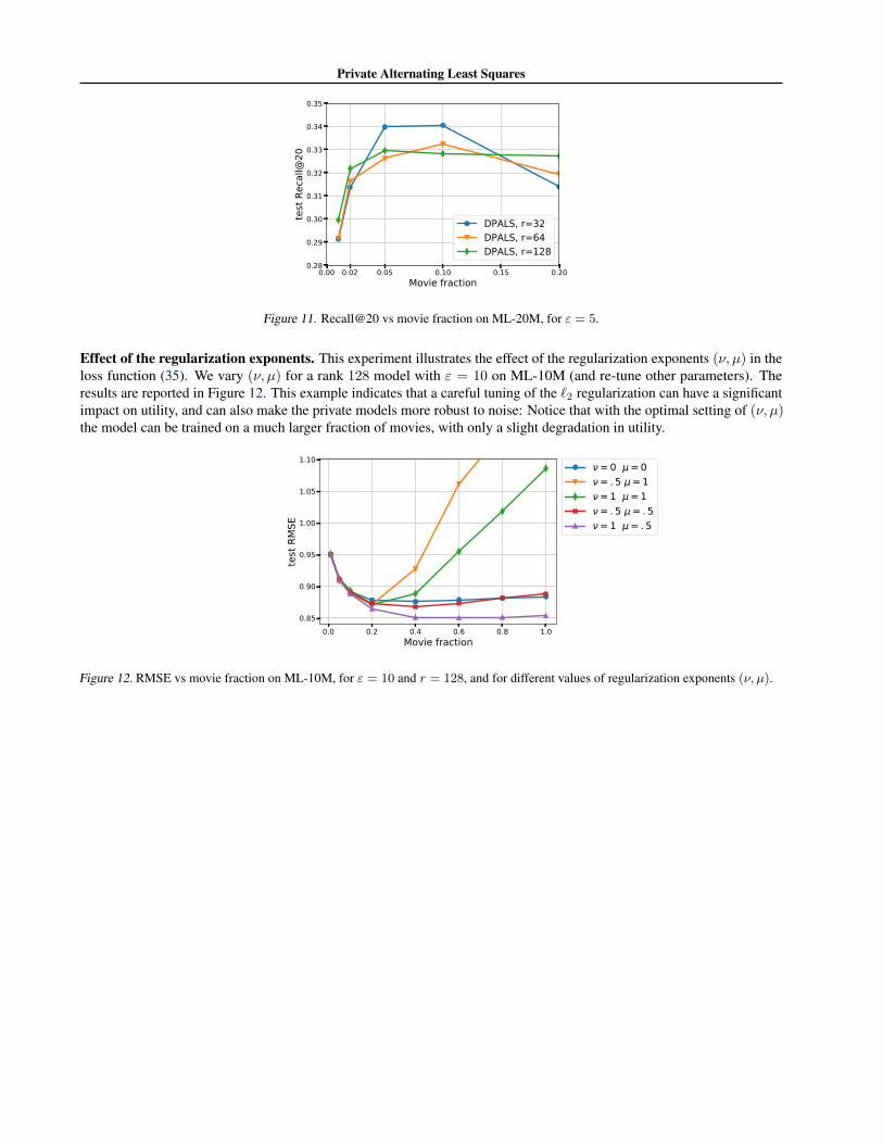
Private Alternating Least Squares
0.00 0.02 0.05 0.10 0.15 0.20Movie fraction
0.28
0.29
0.30
0.31
0.32
0.33
0.34
0.35
test
Rec
all@
20
DPALS, r=32DPALS, r=64DPALS, r=128
Figure 11. Recall@20 vs movie fraction on ML-20M, for ε = 5.
Effect of the regularization exponents. This experiment illustrates the effect of the regularization exponents (ν, µ) in theloss function (35). We vary (ν, µ) for a rank 128 model with ε = 10 on ML-10M (and re-tune other parameters). Theresults are reported in Figure 12. This example indicates that a careful tuning of the `2 regularization can have a significantimpact on utility, and can also make the private models more robust to noise: Notice that with the optimal setting of (ν, µ)the model can be trained on a much larger fraction of movies, with only a slight degradation in utility.
0.0 0.2 0.4 0.6 0.8 1.0Movie fraction
0.85
0.90
0.95
1.00
1.05
1.10
test
RM
SE
ν= 0 μ= 0ν= . 5 μ= 1ν= 1 μ= 1ν= . 5 μ= . 5ν= 1 μ= . 5
Figure 12. RMSE vs movie fraction on ML-10M, for ε = 10 and r = 128, and for different values of regularization exponents (ν, µ).