University of KentuckyUKnowledge

Theses and Dissertations--Computer Science Computer Science

2015

PRIVACY PRESERVING DATA MINING FORNUMERICAL MATRICES, SOCIALNETWORKS, AND BIG DATALian LiuUniversity of Kentucky, lliuc@uky.edu

This Doctoral Dissertation is brought to you for free and open access by the Computer Science at UKnowledge. It has been accepted for inclusion inTheses and Dissertations--Computer Science by an authorized administrator of UKnowledge. For more information, please contactUKnowledge@lsv.uky.edu.

Recommended CitationLiu, Lian, "PRIVACY PRESERVING DATA MINING FOR NUMERICAL MATRICES, SOCIAL NETWORKS, AND BIG DATA"(2015). Theses and Dissertations--Computer Science. Paper 31.http://uknowledge.uky.edu/cs_etds/31

STUDENT AGREEMENT:

I represent that my thesis or dissertation and abstract are my original work. Proper attribution has beengiven to all outside sources. I understand that I am solely responsible for obtaining any needed copyrightpermissions. I have obtained needed written permission statement(s) from the owner(s) of each third-party copyrighted matter to be included in my work, allowing electronic distribution (if such use is notpermitted by the fair use doctrine) which will be submitted to UKnowledge as Additional File.

I hereby grant to The University of Kentucky and its agents the irrevocable, non-exclusive, and royalty-free license to archive and make accessible my work in whole or in part in all forms of media, now orhereafter known. I agree that the document mentioned above may be made available immediately forworldwide access unless an embargo applies.

I retain all other ownership rights to the copyright of my work. I also retain the right to use in futureworks (such as articles or books) all or part of my work. I understand that I am free to register thecopyright to my work.

REVIEW, APPROVAL AND ACCEPTANCE

The document mentioned above has been reviewed and accepted by the student’s advisor, on behalf ofthe advisory committee, and by the Director of Graduate Studies (DGS), on behalf of the program; weverify that this is the final, approved version of the student’s thesis including all changes required by theadvisory committee. The undersigned agree to abide by the statements above.

Lian Liu, Student

Dr. Jun Zhang, Major Professor

Dr. Miroslaw Truszczynski, Director of Graduate Studies

PRIVACY PRESERVING DATA MINING FOR NUMERICAL MATRICES, SOCIALNETWORKS, AND BIG DATA

DISSERTATION

A dissertation submitted in partialfulfillment of the requirements for thedegree of Doctor of Philosophy in the

College of Engineering at theUniversity of Kentucky

ByLian Liu

Lexington, Kentucky

Director: Dr. Jun ZhangProfessor of Computer Science

Lexington, Kentucky 2015

Copyright c© Lian Liu 2015

ABSTRACT OF DISSERTATION

PRIVACY PRESERVING DATA MINING FOR NUMERICAL MATRICES, SOCIALNETWORKS, AND BIG DATA

Motivated by increasing public awareness of possible abuse of confidential information,which is considered as a significant hindrance to the development of e-society, medicaland financial markets, a privacy preserving data mining framework is presented so thatdata owners can carefully process data in order to preserve confidential information andguarantee information functionality within an acceptable boundary.

First, among many privacy-preserving methodologies, as a group of popular techniquesfor achieving a balance between data utility and information privacy, a class of data per-turbation methods add a noise signal, following a statistical distribution, to an originalnumerical matrix. With the help of analysis in eigenspace of perturbed data, the potentialprivacy vulnerability of a popular data perturbation is analyzed in the presence of very littleinformation leakage in privacy-preserving databases. The vulnerability to very little dataleakage is theoretically proved and experimentally illustrated.

Second, in addition to numerical matrices, social networks have played a critical role inmodern e-society. Security and privacy in social networks receive a lot of attention becauseof recent security scandals among some popular social network service providers. So,the need to protect confidential information from being disclosed motivates us to developmultiple privacy-preserving techniques for social networks.

Affinities (or weights) attached to edges are private and can lead to personal securityleakage. To protect privacy of social networks, several algorithms are proposed, includ-ing Gaussian perturbation, greedy algorithm, and probability random walking algorithm.They can quickly modify original data in a large-scale situation, to satisfy different privacyrequirements.

Third, the era of big data is approaching on the horizon in the industrial arena andacademia, as the quantity of collected data is increasing in an exponential fashion. Threeissues are studied in the age of big data with privacy preservation, obtaining a high confi-dence about accuracy of any specific differentially private queries, speedily and accuratelyupdating a private summary of a binary stream with I/O-awareness, and launching a mu-tual private information retrieval for big data. All three issues are handled by two corebackbones, differential privacy and the Chernoff Bound.

KEYWORDS: Privacy Preservation, Data Mining, Social Networks, Big Data, Sampling

Author’s signature: Lian Liu

Date: March 21, 2015

PRIVACY PRESERVING DATA MINING FOR NUMERICAL MATRICES, SOCIALNETWORKS, AND BIG DATA

ByLian Liu

Director of Dissertation: Jun Zhang

Director of Graduate Studies: Miroslaw Truszczynski

Date: March 21, 2015

ACKNOWLEDGMENTS

A long acknowledgement from the bottom of my heart is better off being placed here than

a routine one at the end of my PhD studying periods.

It is extremely unlucky for a 10-month infant to have Poliomyelitis and idiopatHic

scoliosis Diseases (PhD). Even worse, I have no idea who should be blamed for this until

now.

On the other hand, it is also extremely lucky for a handicapped person to pursue a Ph.D.

degree either in China or in the USA. More importantly, I remember the list of persons who

should be appreciated for this through my life, although the list is far from a full one.

The first part of this list definitely includes a lot of my teachers, from my elementary

school to the graduate school, and from China to the Unite States of America.

Mrs. Yu, the first teacher in my elementary school, unhesitatingly accepts me as one of

her students. It is she, a 5-foot-tall and skinny senior lady, who carried me, a 3-foot-6-inch

boy, on her back from the school to the theater to see a cartoon movie on June 1st, 1990.

Mrs. Juan Gao is the Chinese teacher in my elementary school, and her husband, Mr.

Binquan Peng, is the director of the same school. Mrs. Gao leads me to the world of books,

and makes me fall in love with reading for life. In the summer, Mr. Peng teaches me how

to write a good essay at his home and gives me so many free bike rides to the theater later.

Mrs. Yun Li, the Chinese teacher in my high school, always touches my heart in a

motherly manner.

Mrs. Li, who teaches Mathematics in my senior high school, shows me the beauty of

Mathematics in an unbelievable way. One funny thing about her is the following: she is

the first one to teach me that one of my must-have jobs at university is to date a good girl.

But I fail to achieve it until the graduate school in China.

iii

Mrs. Xiaoyun Li, a Physics teacher in my senior high school, gives me so much valu-

able information for my university applications.

Dr. Binxiang Dai is the instructor of Mathematical Analysis I/II/III at the Hunan Uni-

versity in China. His teachings are surely an art since I can always grasp why I need these

theorems and definitions.

Dr. Lihong Huang, my master advisor, generously accepts me to his group and ignites

my ambition to study aboard. He makes me believe that everyone is academically equal,

and the feeling will be enhanced shortly.

Dr. Jun Zhang, my PhD supervisor, inspires and encourages me to conduct research

in the field of privacy preserving data mining, a totally new area to me. In addition to the

mentorship, Dr. Zhang gives me two treasures which will benefit me for life. The first

one is hardwork. I cannot forget that he calls me around 11 pm to discuss a revised draft

and tells me that I can go to his office around 8:30 am the next day if I have any question

about this revision. The second is equality in the academic world. I can always freely argue

anything about a paper or a research topic with him, even if I am wrong in the end.

The second category of this list should go to my relatives. My father, Mr. Shengyan

Liu, and my mother, Mrs. Jujiao Zhang, give birth to me, raise me, educate me, support

me, sponsor me, and more importantly, love me. Although they do not obtain so much

education, they point out the importance of education to me at a very early age.

Wholehearted gratitude should be given to my father-in-law, Mr. Jianhua He, and my

mother-in-law, Mrs. Liqun He, who unconditionally give the apple of their eyes to me. I

would especially express regret to my mother-in-law because I cannot show her anything

before she passes away forever.

Miss. Jiani Liu, my younger sister, is my friend and drives away the lonely feeling from

me, albeit by disputing and even fighting sometimes.

My wife, Mrs. Fang He, is definitely the most important person in my life. She is the

only girl I date with. Like my research on approximation theory, ”the randomly selected

iv

one may be the best one” for approximation and for marriage. I should thank her for endless

love, ever-lasting support, great patience during my graduate study at the University of

Kentucky.

The third group in the list is my committee members and colleagues.

I am deeply indebted to other faculty members of my Advisory Committee, Dr. Jinze

Liu (Department of Computer Science), Dr. Miroslaw Truszczynski (Department of Com-

puter Science), Dr. Caicheng Lu (Department of Electrical and Computer Engineering),

and Dr. Gerry Swan (College of Education) for their insightful comments and invaluable

suggestions on this work.

I want to express my appreciation to my research colleagues from the HiPSCCS and

CMIDA labs at the Department of Computer Science of the University of Kentucky, for

their help, support, interest and valuable hints. Dr. Yin Wang, Dr. Ning Cao, Dr. Dianwei

Han, Mr. Qi Zhuang, Dr. Xuwei Liang, Dr. Changjiang Zhang, Mr. Pengpeng Lin, Dr.

Ruxin Dai, Mr. Xiwei Wang, and Dr. Nirmal Thapa create a friendly working environment

together and give me their helpful discussions and suggestions.

Finally, I would like to repeat that the list is far from a full record, and say ”Thank you

all so much!”

v

TABLE OF CONTENTS

Acknowledgments . . . . . . . . . . . . . . . . . . . . . . . . . . . . . . . . . . . . iii

Table of Contents . . . . . . . . . . . . . . . . . . . . . . . . . . . . . . . . . . . . vi

List of Figures . . . . . . . . . . . . . . . . . . . . . . . . . . . . . . . . . . . . . . viii

List of Tables . . . . . . . . . . . . . . . . . . . . . . . . . . . . . . . . . . . . . . x

Chapter 1 Introduction to Privacy Preserving Data Mining . . . . . . . . . . . . . 11.1 Introduction to PPDM on Numerical Matrices . . . . . . . . . . . . . . . . 11.2 Introduction to PPDM on Social Networks . . . . . . . . . . . . . . . . . . 31.3 Literature Reviews . . . . . . . . . . . . . . . . . . . . . . . . . . . . . . 3

Chapter 2 Privacy Vulnerability with General Perturbation for Numercial Data . . 82.1 Background and Contributions . . . . . . . . . . . . . . . . . . . . . . . . 82.2 Privacy Breach Analysis . . . . . . . . . . . . . . . . . . . . . . . . . . . 92.3 Experimental Results . . . . . . . . . . . . . . . . . . . . . . . . . . . . . 192.4 Summary . . . . . . . . . . . . . . . . . . . . . . . . . . . . . . . . . . . 22

Chapter 3 Wavelet-Based Data Perturbation for Numerical Matrices . . . . . . . . 243.1 Background and Contributions . . . . . . . . . . . . . . . . . . . . . . . . 243.2 Algorithms . . . . . . . . . . . . . . . . . . . . . . . . . . . . . . . . . . 253.3 Normalization . . . . . . . . . . . . . . . . . . . . . . . . . . . . . . . . . 273.4 Experimental Results . . . . . . . . . . . . . . . . . . . . . . . . . . . . . 303.5 Summary . . . . . . . . . . . . . . . . . . . . . . . . . . . . . . . . . . . 32

Chapter 4 Privacy Preservation in Social Networks with Sensitive Edge Weights . 344.1 Background . . . . . . . . . . . . . . . . . . . . . . . . . . . . . . . . . . 344.2 Edge Weight Perturbation . . . . . . . . . . . . . . . . . . . . . . . . . . . 384.3 Experiments . . . . . . . . . . . . . . . . . . . . . . . . . . . . . . . . . . 504.4 Summary . . . . . . . . . . . . . . . . . . . . . . . . . . . . . . . . . . . 57

Chapter 5 Privacy Preservation of Affinities Social Networks via Probabilistic Graph 585.1 Background . . . . . . . . . . . . . . . . . . . . . . . . . . . . . . . . . . 585.2 Data Utility and Privacy . . . . . . . . . . . . . . . . . . . . . . . . . . . . 615.3 Modification Algorithm . . . . . . . . . . . . . . . . . . . . . . . . . . . . 665.4 Experimental Results . . . . . . . . . . . . . . . . . . . . . . . . . . . . . 715.5 Summary . . . . . . . . . . . . . . . . . . . . . . . . . . . . . . . . . . . 77

Chapter 6 Differential Privacy in the Age of Big Data . . . . . . . . . . . . . . . . 796.1 A Roadmap to the Following Chapters and Contributions . . . . . . . . . . 806.2 Preliminaries about Differential Privacy . . . . . . . . . . . . . . . . . . . 82

vi

Chapter 7 A User-Perspective Accuracy Analysis of Differential Privacy . . . . . 947.1 Comparison of d and d . . . . . . . . . . . . . . . . . . . . . . . . . . . . 967.2 Comparison of

∑di and

∑di . . . . . . . . . . . . . . . . . . . . . . . . 97

7.3 Max, Min, Sum, and Mean . . . . . . . . . . . . . . . . . . . . . . . . . . 103

Chapter 8 An I/O-Aware Algorithm for a Differentially Private Mean of a BinaryStream . . . . . . . . . . . . . . . . . . . . . . . . . . . . . . . . . . . 105

8.1 Introduction . . . . . . . . . . . . . . . . . . . . . . . . . . . . . . . . . . 1058.2 Analysis of Previous Methods . . . . . . . . . . . . . . . . . . . . . . . . 1068.3 Private Mean Releasing Scheme . . . . . . . . . . . . . . . . . . . . . . . 1088.4 The Chernoff Bounds . . . . . . . . . . . . . . . . . . . . . . . . . . . . . 112

Chapter 9 Security Information Retrieval on Private Data Sets . . . . . . . . . . . 1189.1 Introduction . . . . . . . . . . . . . . . . . . . . . . . . . . . . . . . . . . 1189.2 Accuracy Analysis of the Naive Solution . . . . . . . . . . . . . . . . . . . 1199.3 Wavelet Transformation of y . . . . . . . . . . . . . . . . . . . . . . . . . 1239.4 Sparsification Strategy for wy . . . . . . . . . . . . . . . . . . . . . . . . . 126

Chapter 10 Future Works . . . . . . . . . . . . . . . . . . . . . . . . . . . . . . . 12810.1 Differential Privacy for Small-Valued Numbers . . . . . . . . . . . . . . . 12810.2 Verification of Differential Privacy . . . . . . . . . . . . . . . . . . . . . . 130

Bibliography . . . . . . . . . . . . . . . . . . . . . . . . . . . . . . . . . . . . . . 133

Vita . . . . . . . . . . . . . . . . . . . . . . . . . . . . . . . . . . . . . . . . . . . 148

vii

LIST OF FIGURES

2.1 Distribution of the singular values of the Bupa dataset during the perturbation. . 202.2 Distribution of the singular values of the Wine dataset during the perturbation. . 21

4.1 Original business network. All nodes in this figure represent either a companyor an agent (supplier) and the edge means a business connection between thetwo entities. The weight of each edge denotes the transaction expense of thecorresponding business connection. . . . . . . . . . . . . . . . . . . . . . . . . 36

4.2 Perturbed business network. . . . . . . . . . . . . . . . . . . . . . . . . . . . 374.3 A simple social network G and the three shortest paths. . . . . . . . . . . . . . 384.4 The perturbed social network G∗ of G in Figure 4.3. Compared to Figure 4.3,

all weights in this figure except w2,3 and w2,5 are perturbed. . . . . . . . . . . . 414.5 The formulization of perturbation purposes. . . . . . . . . . . . . . . . . . . . 444.6 Three different categories of edges. The red bold-faced edges are partially-

visited edges, the black thin edges are non-visited ones, and the blue dashededge is the all-visited edge. . . . . . . . . . . . . . . . . . . . . . . . . . . . . 44

4.7 Perturbation on the non-visited and all-visited edges. . . . . . . . . . . . . . . 454.8 Increasing the weight of the partially-visited edge e2,5. . . . . . . . . . . . . . 464.9 Decreasing the weight of a partially-visited edge e2,5. . . . . . . . . . . . . . . 474.10 Percentage of the perturbed shortest path lengths and weights in the range after

the Gaussian perturbation with σ=0.1 on EIES. . . . . . . . . . . . . . . . . . 514.11 Percentage of the perturbed shortest path lengths and weights in the range after

the Gaussian perturbation with σ=0.15 on EIES. . . . . . . . . . . . . . . . . . 524.12 Percentage of the perturbed shortest path lengths and weights in the range after

the Gaussian perturbation with σ=0.2 on EIES. . . . . . . . . . . . . . . . . . 534.13 Percentage of the perturbed shortest path lengths and weights in the range after

the greedy perturbation with 77% targeted pairs being preserved. . . . . . . . . 544.14 Percentage of the perturbed shortest path lengths and weights in the range after

the greedy perturbation with 54% targeted pairs being preserved. . . . . . . . . 554.15 Percentage of the perturbed shortest path lengths and weights in the range after

the greedy perturbation with 25% targeted pairs being preserved. . . . . . . . . 56

5.1 The original business social network and the modified one. In the modified net-work, the blue edge group and the green edge group satisfy the 4-anonymousprivacy where µ=10. . . . . . . . . . . . . . . . . . . . . . . . . . . . . . . . 64

5.2 The conditions for weight modification of a single edge. . . . . . . . . . . . . . 675.3 The comparison about privacy levels in three sortings and the original case in

the condition of H=10% and µ=10 for the data sets EIES and SYN1. . . . . . . 725.4 The comparison about privacy levels in three sortings and the original case in

the condition of H=10% and µ=10 for the data set SYN2. . . . . . . . . . . . . 735.5 The comparison about the three criteria in three cases in the condition of k=3

and µ=10 for the data sets EIES and SYN1. . . . . . . . . . . . . . . . . . . . 74

viii

5.6 The comparison about the three criteria in three cases in the condition of k=3and µ=10 for the data set SYN2. . . . . . . . . . . . . . . . . . . . . . . . . . 75

5.7 The comparison about the percentage of µ-weighted k-anonymous edges in thecondition of H=10% and µ=10 for the data sets EIES and SYN1. . . . . . . . . 76

5.8 The comparison about the percentage of µ-weighted k-anonymous edges in thecondition of H=10% and µ=10 for the data set SYN2. . . . . . . . . . . . . . . 77

6.1 Three Laplace distributions. . . . . . . . . . . . . . . . . . . . . . . . . . . . . 81

7.1 Histogram for smokers in six areas. . . . . . . . . . . . . . . . . . . . . . . . . 957.2 Mean of Laplace noises. . . . . . . . . . . . . . . . . . . . . . . . . . . . . . 987.3 Mean of Laplace noises. . . . . . . . . . . . . . . . . . . . . . . . . . . . . . 997.4 Sum of Laplace noises. . . . . . . . . . . . . . . . . . . . . . . . . . . . . . . 997.5 Sum of Laplace noises. . . . . . . . . . . . . . . . . . . . . . . . . . . . . . . 100

9.1 1D Haar discrete wavelet decomposition. . . . . . . . . . . . . . . . . . . . . . 1249.2 The workflow of the publication. . . . . . . . . . . . . . . . . . . . . . . . . . 126

ix

LIST OF TABLES

2.1 Percentages of angle preservation between Ak and Ak. . . . . . . . . . . . . . 22

3.1 Performance comparison of SVD and wavelet transformation on WBC. . . . . 313.2 Performance comparison between SVD and wavelet transformation on WDBC. 323.3 Different parameter comparison of SVD and wavelet perturbation. . . . . . . . 33

8.1 Ranges of exponential noises. . . . . . . . . . . . . . . . . . . . . . . . . . . . 115

9.1 Notations. . . . . . . . . . . . . . . . . . . . . . . . . . . . . . . . . . . . . . 120

10.1 Percentages of Laplace samples in/beyond ranges. . . . . . . . . . . . . . . . . 129

x

Chapter 1 Introduction to Privacy Preserving Data Mining

With the widespread availability of digital data in the information age, data collection aswell as data mining are becoming more and more a standard practice whose goal is toefficiently and correctly discover patterns, association rules, or relationships hidden in alarge number of different formats and multiparty data, and then combine the historicalpatterns and the current understanding to predict future trends. Although with such a broadand attractive prospect, data mining techniques undoubtedly face a challenge to their legalsurvivals. That is how to protect the privacy of certain crucial data such as medical records,private financial messages, and homeland security information.

The major spectrum of this dissertation falls in Privacy Preserving Data Mining (PPDM)on numerical matrices, social networks, and big data. It is motivated and inspired by theincreasing public awareness of possible abuse and leakage of confidential information,which is considered as a significant hindrance to the development of e-society, medical andfinancial markets, and technology adoption and advance in homeland security. The mainobjective of this thesis is to develop a set of techniques that data owners can use to pro-cess sensitive data in order to preserve confidential information and guarantee informationfunctionality within an acceptable boundary.

This dissertation is simply divided into two parts. One covers privacy preservation onnumerical matrices and social networks, the other deals with big data. In this chapter, abrief introduction will be demonstrated to cover the first part presented in Chapters 2, 3, 4,and 5. Chapter 6 will give a background for differential privacy in the age of big data, fromconfidence analysis of private queries in Chapter 7 to an I/O- aware private algorithm for abinary stream in Chapter 8 and mutual private information retrieval in Chapter 9. Chapter10 makes two proposals for future privacy research in the era of big data.

1.1 Introduction to PPDM on Numerical Matrices

Generally speaking, data mining, also known as information or knowledge discovery indatabases, is a relatively new field in computer science. It aims at finding valuable andusable patterns, knowledge and information from a large volume of data sets by usinginterdisciplinary methodologies from statistics, machine learning, artificial intelligence,for example.

Even with such a broad and attractive prospect, however, data mining techniques onconfidential data undoubtedly face a challenge to their legal survivals. That is how to pro-tect the privacy of certain crucial data such as medical records, private financial messages,and homeland security information. Although data mining itself has no ethical implica-tions, the functionality of data mining can be applied to discover the relationship betweendifferent implicit informative patterns hidden in unknown domains. This relationship maylead to confidential information leakage through malicious analysis. To satisfy the desiredprivacy requirement, more and more organizations and law enforcements establish a bodyof codes of privacy and security. For example, to comply with the Health Insurance Porta-bility and Accountability Act (HIPAA), individual persons and organizations do not have

1

to reveal their medical data for the public use without the privacy protection guarantee inany case.

Another example could be in commercial data analysis fields. In order to maximizebusiness profit return and to provide better customer services, different business organiza-tions may reach a multiparty agreement that each party is willing to share its own com-mercially processed data with others. The set of processed data can be clustered into var-ious targeted groups, by each business organization whose goal is to implement suitablemarketing strategies. After such classification, the further analyses like decision tree andregression can potentially boost business profits with the aid of statistical analysis. Theoriginal data shared to the partners without identified identities such as SSN will probablyviolate customer’s privacy since those anonymized data can be de-anonymized by auxiliaryinformation from outside contributors [13]. Hence, it is needed to take concrete steps toensure that certain private information in each owner’s data is not disclosed to the otherparties.

For traditional data mining applications such as in the previous commercial case, a lot ofdata to be processed can be easily transformed to numerical format. From this perspective,data mining can smoothly go ahead with the help of some numerical computing techniqueslike matrix manipulation. Among many traditional privacy-preserving methodologies, as agroup of popular techniques for achieving a balance between data utility and informationprivacy, a class of data perturbation methods add certain amount of noise signal, followinga statistical distribution, to the original data as follows:

A = A ∗R + E,

where A is the original numerical data with any dimension, R is an orthogonal matrixwhich has an appropriate dimension with respect to A, and E is a noise matrix followinga certain statistical distribution. In this dissertation, data perturbation’s potential privacyvulnerability is first analyzed in the presence of very little information leakage in privacy-preserving database and data mining based on the eigenspace of the perturbed data undersome constraints. The situation is studied in which data privacy may be compromised withthe leakage of a few original data entries and it will be shown that, in a general perturba-tion model, even the leakage of only one single original data entry may compromise theprivacy of perturbed data in some cases. Chapter 2 theoretically proves and experimentallyillustrates that in this model most data is vulnerable to very little data leakage.

Chapter 3 presents a class of novel privacy-preserving collaborative analysis methodsbased on wavelet transformation instead of the above general noise addition/deletaion.Wavelets are a set of functions which are localized, scaled and well-organized in orderto satisfy certain requirements. Wavelet transformation is widely used in signal processing[35, 44] and noise suppression [147]. With the aid of wavelet analysis, the perturbation isbased on the data property instead of following an independent distribution.

Furthermore, it is needed for some privacy-preserving data perturbation strategies tokeep very good data mining utilities while preserving certain privacy, data statistics areusually not included in the consideration of these techniques. For certain applications, it isnecessary to keep statistical properties so that the perturbed data can be used for statisticalanalysis in addition to the data mining analysis. So a strategy based on wavelet perturba-

2

tion and normalization post-processing is developed to maintain data mining utilities andstatistical properties in addition to the data privacy protection.

1.2 Introduction to PPDM on Social Networks

In addition to traditional data sources, social networks have played a critical role in themodern e-society as well as in anthropology, biology, economics, geography, and psychol-ogy, etc. Security and privacy in social networks receive a lot of attention because of therecent security scandals among some popular social network service providers [62, 93].

A social network is a computer network based graph structure made of entities andconnections between these entities. The entities, or nodes, are abstract representations ofeither individuals or organizations that are connected by links with one or more attributes.The connections, or edges, denote relationships or interactions between these nodes. Socialnetworks typically contain a large amount of private information. The need to protectconfidential, sensitive, and security information from being disclosed motivates researchersto develop privacy-preserving techniques for social networks.

From data mining points of view, unfortunately, data in social networks cannot easilybe manipulated in traditional transformation due to the nature of extreme high-dimensionand large-scale. Faced with the dramatically increasing of social networks, the volume ofnon-traditional data, like social networks, does grow exponentially.

From the privacy preserving perspective, the challenge in social network security studyis twofold. First, it is unknown what information in social networks is confidential andits relationship to personal privacy. For instance, it is argued that affinities (or weights)attached to edges are privacy and they can lead to personal security leakage, in additionto identities privacy in social networks. Second, it is hard to mathematically define andmanipulate data in social networks and quickly process such data to keep its privacy.

Based on the above reasons, new theoretical foundations and corresponding technolo-gies should be proposed to successfully and confidentially discover invaluable informationin non-traditional data domains like social networks with a guarantee of privacy preser-vation within a satisfactory level. New theoretical foundations and methodologies shouldbe fitted into the large-scale computational environment. For example, the secure data inone party probably becomes vulnerable due to data publishing by the other parties. Thispossibility requires researchers to create a unified analysis on large-scale data resided in asmany locations as possible.

1.3 Literature Reviews

Current Status of Traditional Data Privacy Preservation

In the past decade, there have been a large number of privacy-preserving data mining lit-erature. Many researchers attempt to develop techniques to maintain data utilities withoutdisclosing the original data and to produce data analysis results that are as close to thosebased on the original data as possible. Among those techniques, there are two main cat-egories. Methods in the first category modify data mining algorithms so that they allowdata mining operations on distributed datasets without knowing the exact values of the data

3

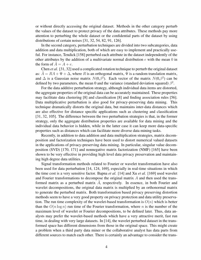
or without directly accessing the original dataset. Methods in the other category perturbthe values of the dataset to protect privacy of the data attributes. These methods pay moreattention to perturbing the whole dataset or the confidential parts of the dataset by usingdistributions of certain noises [31, 32, 54, 82, 91, 126].

In the second category, perturbation techniques are divided into two subcategories, dataaddition and data multiplication, both of which are easy to implement and practically use-ful. For instance, Tendick [158] perturbed each attribute in the dataset independently of theother attributes by the addition of a multivariate normal distribution e with the mean 0 inthe form of A = A+ e.

Chen et al. [31, 32] used a complicated rotation technique to perturb the original datasetas: A = RA+ Ψ + ∆, where R is an orthogonal matrix, Ψ is a random translation matrix,and ∆ is a Gaussian noise matrix N (0,β2). Each vector of the matrix N (0,β2) can bedefined by two parameters, the mean 0 and the variance (standard deviation squared) β2.

For the data additive perturbation strategy, although individual data items are distorted,the aggregate properties of the original data can be accurately maintained. These propertiesmay facilitate data clustering [8] and classification [8] and finding association rules [56].Data multiplicative perturbation is also good for privacy-preserving data mining. Thistechnique dramatically distorts the original data, but maintains inter-data distances whichare also effective for distance specific applications such as clustering and classification[31, 32, 105]. The difference between the two perturbation strategies is that, in the formerstrategy, only the aggregate distribution properties are available for data mining and theindividual data behavior is hidden, while in the latter case it can keep more data-specificproperties such as distances which can facilitate more diverse data mining tasks.

Recently, in addition to data addition and data multiplication strategies, matrix decom-position and factorization techniques have been used to distort numerical valued datasetsin the applications of privacy-preserving data mining. In particular, singular value decom-position (SVD) [170, 171] and nonnegative matrix factorization (NMF) [165] have beenshown to be very effective in providing high level data privacy preservation and maintain-ing high degree data utilities.

Signal transformation methods related to Fourier or wavelet transformation have alsobeen used for data perturbation [14, 124, 169], especially in real-time situations in whichthe time cost is a very sensitive factor. Bapna et al. [14] and Xu et al. [169] used waveletand Fourier transformations to decompose the original matrix A and then used the trans-formed matrix as a perturbed matrix A, respectively. In essence, in both Fourier andwavelet decompositions, the original data matrix is multiplied by an orthonormal matrixto generate the perturbed matrix. Both transformation based privacy preserving distortionmethods seem to have a very good property on privacy protection and data utility preserva-tion. The run time complexity of the wavelet-based transformation is O(n) which is betterthan the O(n log n) run time of the Fourier transformation, where n is the number of themaximum level of wavelet or Fourier decompositions, to be defined later. Thus, data an-alysts may prefer the wavelet-based methods which have a very attractive merit, fast runtime, in dealing with very large datasets. In [14], the wavelet perturbed dataset in the trans-formed space has different dimensions from those in the original space. This might createa problem when a third party data miner or the collaborative analyst has data parts fromdifferent sources to match each other. There is certainly an advantage to consider the trans-

4

formed dataset that keeps the same dimension as the original dataset in the collaborativedata analysis situation.

For the statistical property maintenance, some publications [125, 137] focus on keepingthe data privacy and data statistics. But these techniques generate perturbed values whichare purely consistent with the original statistical distribution and independent of originaldata. Because the perturbed data is independent of the original value, data mining utilitiesmay not be perfectly preserved in some cases.

For multiparty data mining, there are two cooperative analysis directions. The first oneis referred to as vertically collaborative analysis [159] in which the databases of differ-ent companies have exactly the same customer set but the attribute sets of the datasets aredifferent. The second one is called horizontally collaborative analysis [114] where the at-tribute set of the multiparty database is the same but companies target at different customersets. In both scenarios, the collaborative analysis is considered as an essential approach togaining more comprehensive knowledge from the combined databases.

In recent years, however, it is noticed that the perturbed or distorted datasets from cer-tain data perturbation techniques may not be safe if an attacker has some background in-formation about the original datasets [71, 72, 91, 86, 111]. In practice, it is unlikely that anattacker has no idea about the original dataset other than the public perturbed version. Thecommon sense, statistical measure, reference, and even a small amount of leakage may dra-matically help the attacker weaken the privacy of the dataset. Kargupta et al. [92] showedthat it is highly possible to differentiate the original true values from the additively per-turbed data. Guo and Wu [71, 72] calculated a useful upper bound and lower bound aboutthe difference between the original dataset and the estimated dataset which is computedfrom the perturbed dataset by spectral filtering techniques. Aggarwal [5] presented that, inthe data additive perturbation, the privacy is susceptible from a known public dataset in ahigh dimensional space.

Their works have mentioned the use of background information probably possessed bythe attacker in either data additive perturbation or multiplicative strategies, and they neededmuch more background information to support their privacy breach analysis. In Chapter2, attention will be paid to privacy breach analysis of the perturbed dataset with one singlebackground record in a general data perturbation.

Besides, there are several classes of data distortion or perturbation methods. For ex-ample, one class is focused on data anonymization [117, 153, 162, 164, 181]. Briefly,on one hand, the data anonymization strategy removes certain parts of the dataset such asunique and confidential identifiers, e.g., social security numbers or driver’s license num-bers or credit card numbers. Sweeney [152] demonstrated that this strategy may not besafe to guarantee identification privacy because the intruders can discover certain secretinformation by exploiting relationships among other attributes. On the other hand, the datarandomization perturbation preserves data utilities such as patterns and association rulesby using the additive random noise. However, Kargupta et al. [92] showed that it is highlypossible to differentiate the original true values from the additive randomization noise per-turbed datasets.

5

Current Status of Social Networks Privacy Preservation

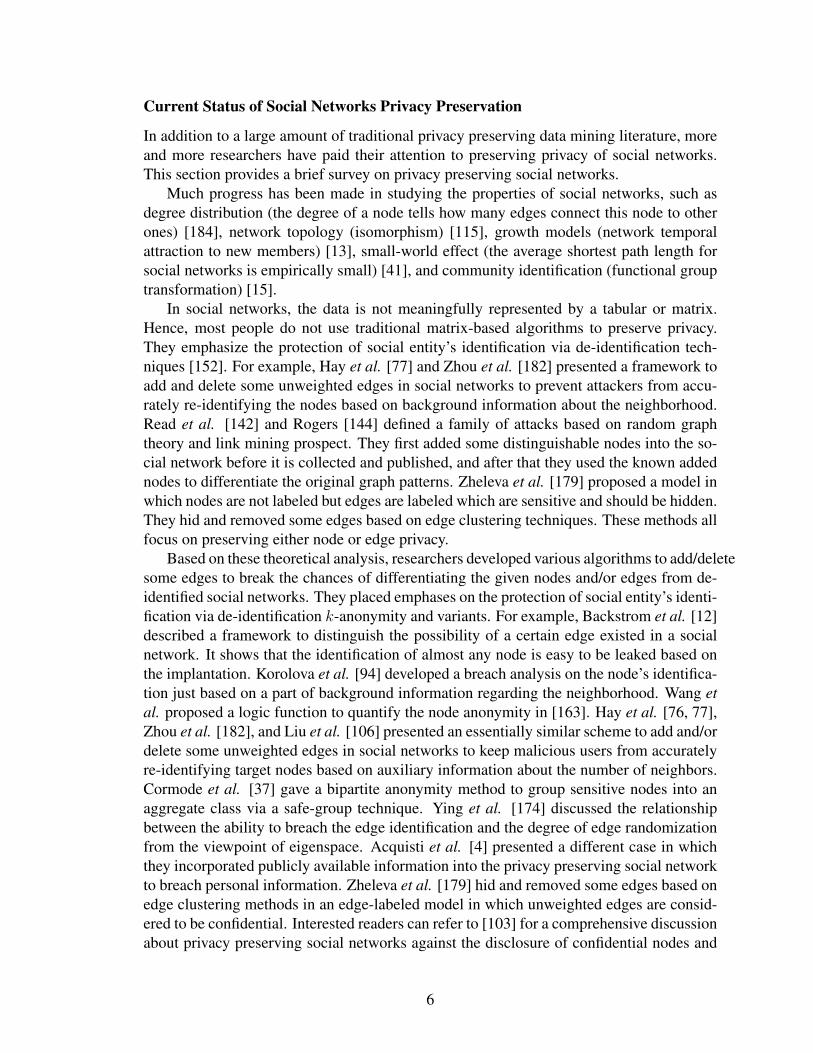
In addition to a large amount of traditional privacy preserving data mining literature, moreand more researchers have paid their attention to preserving privacy of social networks.This section provides a brief survey on privacy preserving social networks.

Much progress has been made in studying the properties of social networks, such asdegree distribution (the degree of a node tells how many edges connect this node to otherones) [184], network topology (isomorphism) [115], growth models (network temporalattraction to new members) [13], small-world effect (the average shortest path length forsocial networks is empirically small) [41], and community identification (functional grouptransformation) [15].

In social networks, the data is not meaningfully represented by a tabular or matrix.Hence, most people do not use traditional matrix-based algorithms to preserve privacy.They emphasize the protection of social entity’s identification via de-identification tech-niques [152]. For example, Hay et al. [77] and Zhou et al. [182] presented a framework toadd and delete some unweighted edges in social networks to prevent attackers from accu-rately re-identifying the nodes based on background information about the neighborhood.Read et al. [142] and Rogers [144] defined a family of attacks based on random graphtheory and link mining prospect. They first added some distinguishable nodes into the so-cial network before it is collected and published, and after that they used the known addednodes to differentiate the original graph patterns. Zheleva et al. [179] proposed a model inwhich nodes are not labeled but edges are labeled which are sensitive and should be hidden.They hid and removed some edges based on edge clustering techniques. These methods allfocus on preserving either node or edge privacy.

Based on these theoretical analysis, researchers developed various algorithms to add/deletesome edges to break the chances of differentiating the given nodes and/or edges from de-identified social networks. They placed emphases on the protection of social entity’s identi-fication via de-identification k-anonymity and variants. For example, Backstrom et al. [12]described a framework to distinguish the possibility of a certain edge existed in a socialnetwork. It shows that the identification of almost any node is easy to be leaked based onthe implantation. Korolova et al. [94] developed a breach analysis on the node’s identifica-tion just based on a part of background information regarding the neighborhood. Wang etal. proposed a logic function to quantify the node anonymity in [163]. Hay et al. [76, 77],Zhou et al. [182], and Liu et al. [106] presented an essentially similar scheme to add and/ordelete some unweighted edges in social networks to keep malicious users from accuratelyre-identifying target nodes based on auxiliary information about the number of neighbors.Cormode et al. [37] gave a bipartite anonymity method to group sensitive nodes into anaggregate class via a safe-group technique. Ying et al. [174] discussed the relationshipbetween the ability to breach the edge identification and the degree of edge randomizationfrom the viewpoint of eigenspace. Acquisti et al. [4] presented a different case in whichthey incorporated publicly available information into the privacy preserving social networkto breach personal information. Zheleva et al. [179] hid and removed some edges based onedge clustering methods in an edge-labeled model in which unweighted edges are consid-ered to be confidential. Interested readers can refer to [103] for a comprehensive discussionabout privacy preserving social networks against the disclosure of confidential nodes and

6

links. For a survey about privacy preserving social networks to date, readers can take alook at [183].

Copyright c© Lian Liu, 2015.

7

Chapter 2 Privacy Vulnerability with General Perturbation for Numercial Data

The issue of data privacy is considered a significant hindrance to the development andindustrial applications of database publishing and data mining techniques. Among manyprivacy-preserving methodologies, data perturbation is a popular technique for achieving abalance between data utility and information privacy. It is known that the attacker’s back-ground information about the original data can play a significant role in breaching dataprivacy. In this chapter, data perturbation’s potential privacy vulnerability will be analyzedin the presence of known background information in privacy-preserving database publish-ing and data mining based on the eigenspace of the perturbed data under some constraints.The situation is studied in which data privacy may be compromised with the leakage ofa few original data records. It first shows that additive perturbation preserves the anglebetween data records during the perturbation. Based on this angle-preservation property,in a general perturbation model even the leakage of only one single original data probablydegrades the privacy of perturbed data in some cases. Theoretical and experimental resultsshow that a general data perturbation model is vulnerable from this type of backgroundprivacy breach.

2.1 Background and Contributions

Database publishing and data mining techniques enable the discovery of valuable data pat-terns and knowledge in collected and shared data and increase business profitability andenhance national security. The precondition of useful data analysis is the collection oflarge amounts of data, which has been made possible by the recent availability of relativelyinexpensive means of large scale electronic data collections. On the other hand, users alsoface the challenge of controlling the level of private information disclosure and securingcertain confidential patterns within the data, without noticeably affecting the utilities of thedata for intended purposes of analysis. The difficulty of data security increases consid-erably if users aim to achieve the goal of maintaining confidential data privacy and datautility at the same time, in privacy-preserving database publishing and data mining.

Data privacy and security can be compromised from many different ways, both insideand outside the data collection organizations. Even within the data collection organiza-tions, different people are assigned different levels of trustworthiness, usually through theprivileges of the computer accounts they use. To protect data privacy and security frombeing compromised intentionally or unintentionally, it is preferable that data is prepro-cessed appropriately before it is distributed for analysis or made to the public. One of themost useful data preprocessing techniques is data perturbation (or data randomization [7]),which attempts to perturb the true values of the original data in an effort to preserve thedata privacy and data utility.

In this chapter, data privacy vulnerability will be theoretically analyzed in the presenceof background information and strategies will be developed to breach original informationfrom the perturbed data. Background information is one or more original data records ex-actly known by an attacker. Such background information may be used by the attacker

8

to compromise other records in the original data, with the availability of the public per-turbed data. Suppose a fictitious situation where an organization collects many recordsfrom hundreds of thousands of persons including Bob, and compiles such records into awell-defined dataset as the original matrix A and distorts the original dataset to a perturbeddataset as a matrix A and finally publishes this perturbed dataset A to the public. For Bob,he knows the exact values of his original record in A, the corresponding perturbed valuesof his record, and the whole perturbed dataset A. This chapter considers the theoreticalpossibility that Bob may use his original data values and the perturbed dataset to breachthe privacy of other records in the original dataset.

Contributions in this chapter are fivefold as follows:(1). In general, there are two major techniques for data perturbation, data additive

perturbation and data orthogonal multiplicative perturbation (the data multiplication is thesame as the data orthogonal multiplication in this chapter unless otherwise stated explic-itly). A property of this type of data multiplication is that it is a rotation operation whichwill keep the angle of inter-data during the perturbation. The first contribution shows thatthe data additive perturbation also has this property under some conditions.

(2). Although many literature have shown the vulnerability of data additive perturbation[7, 11, 91, 111] and data multiplicative perturbation [71, 72, 104] from different viewpoints,respectively. The privacy analysis in this chapter is based on a general perturbation modelwhich consists of data additive and multiplicative perturbation techniques together. In otherwords, the potential vulnerability of privacy can be applied to both perturbation methods.

(3). Previous privacy breach analysis [7, 6, 54, 104] are practical and useful with the aidof many more known samples. But the results show that even the leakage of one single datarecord (sample) probably causes the failure of privacy preservation under some conditions.

(4). In most privacy analysis techniques, there exist some assumptions to be knownexplicitly after perturbation, such as the standard deviation of additive noise [7, 6], the as-sumption of privacy analysis is minimized to one known original data record as well as thecorresponding perturbed data records. Based on this information, under some constraints,other original data records can be breached from the public perturbed data records.

(5). A practical and simple method is proposed to analyze and breach the privacy ofperturbed data in some cases.

2.2 Privacy Breach Analysis

This section first presents a general data perturbation model, explains why different dataperturbation algorithms can fall into this model, gives some useful mathematical prepara-tions, and generalizes notations.

Data Perturbation Model

To generalize the perturbation techniques to essentially cover additive and multiplicativestrategies discussed previously as well as many other methods which can be obtained froma general model to perform the perturbation process on the original datasets, a theoreticalgeneral data perturbation model is defined as follows:

A = AR + E, (2.1)

9

where A is an n ∗ m original numerical matrix that presents n original records in an mattribute space, A is the corresponding perturbed data, R is an orthogonal matrix and E isa Gaussian noise matrix with the mean 0 and an arbitrary variance β2.

For a record a=(a1, ..., am) in the original database A, data additive perturbation gen-erates a same size randomization perturbation (or noise) vector e=(e1, ..., em), and eachentry ei in this vector is drawn from a distribution denoted by f(e) which has a standarddeviation β and a mean 0. So the perturbed version for this original record is a=(a1, ...,am)= (a1 + e1, ..., am + em). In most cases, the distribution f(e) is defined as

f(e) =1√2πβ

exp(− e2

2β2).

From the matrix viewpoint, this data additive perturbation with that distribution isequivalent to

A = A+ E.

Here E is a Gaussian matrix with the mean 0 and the variance β2.Data multiplicative perturbation usually transforms the original data from the original

data space Rm to another data space Rd (d ≤ m). It first generates an orthogonal basis(R1, ..., Rd) (Ri is an m ∗ 1 vector). Then for individual original vector a=(a1, ..., am), theperturbed version a=(a1, ..., ad)= (a ∗ R1, ..., a ∗ Rd). So, for all original data records, thedata multiplicative perturbation is

A = AR.

Therefore, the general data perturbation model (2.1) can be considered as a combinationof data addition and data multiplication from the previous analysis.

Equation (2.1) seems to first perturb the original data by multiplication and then byaddition. A similar general perturbation model is given which first perturbs the originaldata by addition and then by multiplication as follows:

A = (A+ E)R. (2.2)

Note that Equation (2.2) can be expanded to A = AR + ER, and the multiplication of aGaussian matrix and an orthogonal matrix ER is still a Gaussian matrix. Equation (2.2)is therefore equivalent to Equation (2.1). So the order of data addition and multiplicationdoes not matter much, and Equation (2.1) is chosen as the prototype of privacy analysis.

Singular Value Decomposition

A useful tool in the data analysis, Singular Value Decomposition (SVD), is a popular matrixfactorization method in matrix computation and is widely used in data mining and infor-mation retrieval. It has been used to reduce the dimensionality of databases in practice andremove the noise in noisy databases [17]. The use of SVD techniques in data perturbationfor privacy-preserving data mining is proposed in [170, 171].

The SVD of the original n ∗m data matrix A is written as

A = USV T . (2.3)

10

Here U is an n∗n orthonormal matrix, S = diag[σ1, ..., σs], where s = min(n,m), withoutthe loss of generality, and nonnegative diagonal entries σis are in a non-increasing order.The diagonal entries σ1, ..., σs are called the singular values. And V T is also an orthonormalmatrix with dimension m ∗m. The number of nonzero diagonal entries of S is equal to therank of the matrix A.

DefineAk = UkSkV

Tk , for a positive integer k ≤ min(n,m),

where Uk only contains the first k columns of U , Sk contains the first k nonzero singularvalues of S, and V T

k contains the first k rows of V T . Obviously, the rank of the matrix Akis k, and Ak is often called the rank-k truncated SVD. Ak has a well-known property thatit is the best k-dimensional (rank-k) approximation of A in terms of the Frobenius norm[69].

In information retrieval, Ek = A - Ak can be considered as the noise of the originaldata matrix. In privacy-preserving data mining, Ak can be used as a perturbed version ofA [170, 171]. So, Ak represents a good approximation which keeps similar patterns of A,while it provides protection for data privacy [170, 171].

Stability of Angle Preservation

For simplicity, in the following discussion, Matlab notations are used to represent matrixentries and rows, respectively.

A the original matrixA the perturbed matrix

Ai,j the entry (i,j) of AAi,: the i-th row of A, simplified as Ai

Ai1:i2,j1:j2 the submatrix of A from the i1-th row to thei2-th row and from the j1-th column to thej2-th column

ai Ai ∗ VkAik the i-th row of Ak as in Theorem 2.2.2

In the following contents, ‖ · ‖ is referred to as the 2- norm (Euclidean norm) unlessotherwise explicitly stated.

The major work of this chapter shows that the attacker has a high possibility to figureout the other original matrix records based on one background record which is an originalmatrix record exactly known by this attacker. From the mathematical viewpoint, the per-turbation model in Equation (2.1) preserves not only the angles between the entire rowsof the original dataset and those of the perturbed dataset, but also the angles between thesubsets of the entire original rows and the corresponding perturbed counterparts during theperturbation.

Lemma 2.2.1. [69] If R is an orthogonal matrix of appropriate dimension, then for anymatrix A,

‖AR‖ = ‖RA‖ = ‖A‖.

11

Lemma 2.2.1 obviously shows that multiplying the original matrix by an orthogonalmatrix does not change the norm. Geometrically, orthogonal matrix multiplication is arotation on all original data such that the inter-data distances and angles are perfectly kept.So, it is known that data multiplicative perturbation can maintain the properties of originalinter-data distances and angles.

Firstly it will be shown that not only the data multiplicative perturbation (A = AR),but also the data additive perturbation (A = A + E) will maintain the inter-data distancesand angles in some cases.

Lemma 2.2.2. If the singular value decomposition of the matrix A is

A = USV T ,

then the following equations hold:

1. AV=US,

2. ‖Ai‖=‖U iS‖,

3. ‖AiVk‖=‖U iSk‖, there Sk is an n ∗m diagonal matrix which only contains the firstk singular values of S.

The proof of this lemma is straightforward. The purpose of the Lemma 2.2.2 is to showthat the norm of an original data record Ai can be represented by the norm of the multi-plication of two SVD-based factorization matrices U i ∗ S which is useful in the followingtheorems.

Theorem 2.2.1. Let A and A = A+ E be n ∗m real matrices, and

A = USV T , A = U SV T

be the SVDs of A and A, respectively.Let

Ak = UkSkVTk , Ak = UkSkV

Tk

be the rank-k best approximations to A and A, respectively.Assume that ‖E‖ ≤ (σk − σk+1) and ‖E‖ ≤ σk, where σk and σk are the k-th singular

values of A and A, respectively.

Defineai = AiVk, a

i = AiVk, and ei = EiVk.

Then‖ai‖ ≈ ‖Ai‖ and ‖ei‖ ≤ ‖ai‖.

12

Proof.

‖ai‖ = ‖Ai ∗ Vk‖= ‖U i ∗ Sk‖ (Lemma 2.2.2.3)

≈ ‖U i ∗ S‖ (∵ σk+1 is small relative tok∑i=1

σi)

= ‖Ai‖. (Lemma 2.2.2.2)

SVD of E is defined as E = UESEVTE , and SE = diag(σ1

E, σ2E, ..., σ

mE ). Since ‖E‖ =

σ1E ≤ σk, the following holds

‖Ei‖2 = ‖U iESE‖2 (Lemma 2.2.2.2)

=m∑j=1

(U ijE )2 ∗ (σjE)2

≤m∑j=1

(U ijE )2 ∗ (σ1

E)2

= (σ1E)2, (∵ U i

E is an unitary vector)≤ (σk)

2, (∵ ‖E‖ = σ1E ≤ σk)

=m∑j=1

(U ij)2 ∗ (σk)2

≤m∑j=1

(U ij)2 ∗ (σj)2, (∵ σk ≤ σ1, ..., σk−1)

= ‖U iSV T‖2

= ‖Ai‖2. (2.4)

Then from Inequality (2.4), it is easy to obtain ‖ei‖ ≤ ‖ai‖.

As in the data additive perturbation (A = A+E), if the additive perturbationE satisfiestwo conditions (‖E‖ ≤ (σk − σk+1) and ‖E‖ ≤ σk), the additive perturbation can bebounded by the original data (‖ei‖ ≤ ‖ai‖). Since only the perturbed data A and σiare known to the public but the original data A, ai and σi are not known to the public,these two conditions cannot be practically used to bound the additive perturbation. But apractical method will be presented to accurately approximate ‖E‖ and σi from the knownperturbed data later. Even approximations for ‖E‖ and σi can be obtained to verify thesatisfaction of the two conditions, the original data, ai, is unknown to the attacker, so it isstill impossible to bound the additive perturbation practically. Actually, the major purposeof Theorem 2.2.1 is to show that if the two conditions (‖E‖ ≤ (σk−σk+1) and ‖E‖ ≤ σk)are satisfied, the two bounds (‖ai‖ ≈ ‖Ai‖ and ‖ei‖ ≤ ‖ai‖) are automatically satisfiedwhich are the basis of the Theorem 2.2.2.

Corollary 2.2.1. Let A and A = A + E be n ∗ m real matrices. Assume that ‖E‖ ≤(σk − σk+1) and ‖E‖ ≤ σk. Assume ai,j1:j2 = Ai,j1:j2V j1:j2,:

k , ai,j1:j2 = Ai,j1:j2V j1:j2,:k , and

13

ei,j1:j2 = Ei,j1:j2V j1:j2,:k .

Then‖ai,j1:j2‖ ≈ ‖Ai,j1:j2‖ and ‖ei,j1:j2‖ ≤ ‖ai,j1:j2‖.

Corollary 2.2.1 is a subset version of Theorem 2.2.1. For an individual original datarecordAi=(Ai,1, ..., Ai,m), the corresponding perturbed version Ai=(Ai,1, ..., Ai,m)= (Ai,1 +Ei,1, ..., Ai,m + Ei,m) is the sum of the original data record and the additive perturbation.Theorem 2.2.1 says that if the two conditions are satisfied, then the entire row additiveperturbation (Ei,1, ..., Ei,m) can be bounded by the entire original data record. WhileCorollary 2.2.1 says that if the two conditions are satisfied, then the subset of the entirerow additive perturbation can also be bounded by the corresponding subset of the entireoriginal data record. The mathematical proof is very similar to the proof of Theorem 2.2.1.For example, it just needs to replace ai, ai, and ei by ai,j , ai,j and ei,j (j is in j1:j2),respectively.

Theorem 2.2.2. [11] LetA and A = A+E be n∗m real matrices andR be an orthogonalmatrix. Assume that ‖E‖ ≤ (σk − σk+1) and ‖E‖ ≤ σk. ai, ai and ei are defined as inTheorem 2.2.1. Then

‖ai −Rai‖ � ‖ai‖ and ‖Aik − Aik‖ � ‖Aik‖.Theorem 2.2.2 establishes a link between the original data Aik and the perturbed data

Aik and bounds the difference between them. Ai and Ai are the i-th original data recordand the corresponding i-th perturbed data record, respectively. Aik is the projection of Ai

on the major k-truncated eigenspace of the original data. Aik is the projection of Ai on themajor k-truncated eigenspace of the perturbed data (it will be discussed as how to selecta detailed value of k at the end of this section). In detail, Theorem 2.2.2 shows that thenorm of the difference between Aik and Aik is much smaller than the norm of Aik, whichmay imply that the angle between Aik and Aik is very small and hence Aik and Aik are closeto each other.

Theorem 2.2.2 is a simplified version of Theorem 2 in [11] which needs to verify theconditions ‖ai‖ ≈ ‖Ai‖ and ‖ei‖ ≤ ‖ai‖. If the conditions are met, Theorem 2 in [11]is true. However, in practice, Ai, ei and ai are not known, it is not practical to verifythese conditions. Based on Theorem 2.2.1, these conditions will be simplified to verify if‖E‖ ≤ σk and ‖E‖ ≤ (σk − σk+1) instead of ‖ai‖ ≈ ‖Ai‖ and ‖ei‖ ≤ ‖ai‖. If ‖E‖ ≤ σkand ‖E‖ ≤ (σk − σk+1), Theorem 2 in [11] as well as the simplified version, Theorem2.2.2 in this chapter, are always true. Later, the discussion will be extended to how toverify ‖E‖ ≤ σk and ‖E‖ ≤ (σk − σk+1) in practice. The details of proof of Theorem2.2.2 can be found in [11].

Based on Theorem 2.2.2, its subset variant is straightforward as the following corollary.

Corollary 2.2.2. Let A and A = A + E be n ∗ m real matrices. Assume that ‖E‖ ≤(σk − σk+1) and ‖E‖ ≤ σk. ai,j1:j2 , ai,j1:j2 , and ei,j1:j2 are defined as in Corollary 2.2.1.Then

‖ai,j1:j2 −Rai,j1:j2‖ � ‖ai,j1:j2‖,and

‖Ai,j1:j2k − Ai,j1:j2

k ‖ � ‖Ai,j1:j2k ‖.

14

Corollary 2.2.2 says that if the two conditions are satisfied, then the subset of the entirerow additive perturbation can also be bounded by the corresponding subset of the originaldata records.

Although Theorem 2.2.2 and Corollary 2.2.2 present a fact that the norm of the differ-ence of the original data and the corresponding perturbed data is much smaller than thenorm of the original data, the original data and its norm are unknown. So the bounds arenot practically useful. But the theoretical bound can be used to show the angle preservationof data additive perturbation.

Based on Theorem 2.2.2 and Corollary 2.2.2, a connection will be established betweenan original data pair and a perturbed data pair, as in the next corollary.

Corollary 2.2.3. Let A and A = A+E be n ∗m real matrices. If ‖E‖ ≤ (σk−σk+1) and‖E‖ ≤ σk, then

1. [11] ‖∠(Apk, Aqk)− ∠(Apk, A

qk)‖ ≤ ε,

2. ‖∠(Ap,j1:j2k , Aq,j1:j2

k )− ∠(Ap,j1:j2k , Aq,j1:j2

k )‖ ≤ ε.

Here, Apk (resp. Aqk) is the p-th (resp. q-th) row of Ak, ε is a small positive number, and∠(Apk, A

qk) denotes the angle between Apk and Aqk (the p-th row and q-th row of Ak).

Corollary 2.2.3 is the main theoretical analysis results on data perturbation privacy. Forexample, according to Corollary 2.2.3.1 ‖∠(Apk, A

qk)−∠(Apk, A

qk)‖ ≤ ε, Ap and Aq are the

p-th and q-th original data records, respectively, Ap and Aq are the corresponding perturbeddata records, respectively. Briefly, Apk is the projection of Ap on the major k-truncatedeigenspace of the original data, and Apk is the projection of Ap on the major k-truncatedeigenspace of the perturbed data. As in the data additive perturbation (A=A + E), theangle between inter-original-data ∠(Apk, A

qk) is very close to that of the inter-perturbed-

data ∠(Apk, Aqk) (Corollary 2.2.3.1), so are those of the corresponding subsets (Corollary

2.2.3.2).Based on Corollary 2.2.3.1, ‖∠(Apk, A

qk)−∠(Apk, A

qk)‖ ≤ ε, it follows that ∠(Apk, A

qk) ≈

∠(Apk, Aqk). In the data additive perturbation A = A+ E, the inter-data angle, under some

conditions, is closely preserved.Secondly in the general perturbation model as in Equation (2.1) A = AR + E, the

inter-data angle is also preserved.

Proposition 2.2.1. [69] For any matrix A, if R is an orthogonal matrix, then A = ARdoes not change the angle between any data records of A.

The proof is very simple and can be found in many books on matrix algorithms. Fromthis proposition, the multiplication of the original matrix and an orthogonal matrix doesnot change the angle of any records of the original matrix. The first part of the generalperturbation model in Equation (2.1), AR, does not change the angle distribution of therecords of the original matrix A. Intuitively, the general perturbation model A = AR + Ecan be considered as a two-step perturbation. The first step is data multiplicative perturba-tion, the second one is data additive process. The multiplication of the original data matrixand an orthogonal matrix does not change the inter-data angle according to Proposition

15

2.2.1. Based on Corollary 2.2.3, data additive perturbation also preserves the angle of datarecords during the process. Therefore, the combination of this proposition and Corollary2.2.3 can prove that the inter-data angle is preserved in this general perturbation model.The skeleton of the proof is as follows. For the general perturbation model A = AR+E,AR can preserve the inter-data angle by Proposition 2.2.1. Based on AR, AR+E does notchange the angle too much according to Corollary 2.2.3. Hence, the angle between A andA is preserved within a boundary under the conditions ‖E‖ ≤ (σk − σk+1) and ‖E‖ ≤ σk.

Although the property of angle preservation in the general perturbation model is proved,what hackers want to breach is the detailed values of the original data records rather theinter-data angles. In the following a strategy is developed to breach the detailed values ofentries of some original data records.

Lemma 2.2.3. If the angle of two vectors X=(x1, ..., xm) and Y =(y1, ..., ym) is very small,the two vectors are highly possible to have similar vector entries.

Proof.

cos∠(X, Y ) =XY T

‖X‖‖Y ‖=

x1y1 + ...+ xmym√x2

1 + ...+ x2m

√y2

1 + ...+ y2m

.

Because the angle of the two vectors X and Y is very small, cos∠(X, Y ) ≈ 1 as follows:

x1y1 + ...+ xmym√x2

1 + ...+ x2m

√y2

1 + ...+ y2m

≈ 1.

Expand the above equation and cancel the common items,

2x1y1x2y2 + ...+ 2xm−1ym−1xmym ≈ x21y

22 + ...+ x2

my2m−1 (2.5)

Equation (2.5) is satisfied if and only if xiyj ≈ xjyi(i, j = 1, ...,m, i 6= j). Given thevarious scales of different dimensions, it can be further concluded that it is highly possiblethat Equation (2.5) is satisfied if and only if xi ≈ yi(i = 1, ...,m).

With the aid of Lemma 2.2.3, the angle preservation presented in Corollary 2.2.3 isuseful for privacy breach analysis.

In addition to the privacy analysis of angle preservation of the general data perturba-tion model, the detailed values of other original data records can be found based on onebackground original data in some cases. For example, it is assumed that the attacher Bobknows one background original data (Ap) and its corresponding perturbed version (Ap).If he can find out another perturbed data (Aq) which has a very small angle with Ap, ac-cording to Corollary 2.2.3.1 (‖∠(Apk, A

qk) − ∠(Apk, A

qk)‖ ≤ ε), it is highly possible, under

the two conditions, that the angle between the original data Apk and Aqk is also very small.According to Lemma 2.2.3, the small angle of the original data Apk and Aqk means that Aq

is very similar to Ap which is known to Bob. So every entry of another original data Aq isbreached. In some cases, although two entire records are not similar, the subsets of the two

16

entire original records may be similar and it still can breach the similar subsets accordingto Corollary 2.2.3.

This example shows that using a single background data as well as the perturbed datacan breach other similar original data. Furthermore, privacy violation will be shown ifBob knows more than a single background original data and the corresponding perturbedversion. It should be noted that this breach algorithm has one drawback. If there is no datain the original space which is similar to the known single background data, e.g., the singlebackground data is an outlier, the breach algorithm cannot hack other perturbed data.

Definition 2.2.1. A set of background original data records, Db, and its correspondingperturbed data records, Db, are the data records which are known to the attackers likeBob. In other words, Bob knows the exact values of all Ai (Ai ∈ Db) and all Ai (Ai ∈ Db).

Theorem 2.2.3. If the number of data in Db is not less than the number of features dimen-sion (or matrix column dimension m), |Db| ≥ m, and the two conditions as in Corollary2.2.3 are satisfied, all other original data are susceptible to this privacy vulnerability.

Theorem 2.2.3 is straightforward and obvious. As an example, there are totally 10 datarecords to be perturbed by the general perturbation model and each record has 4 features(n=10, m=4). Unfortunately, the attacker Bob knows 4 original data records (Db) and theircorresponding perturbed data records (Db). For simplicity, assume that Bob knows A1, A2,A3, A4, A1, A2, A3, and A4. Based on Db and Db, the remaining 6 original data recordscan be also approximated.

For an unknown dataA5, its 4 entries like 4 unknown variables. According to Corollary2.2.3,

‖∠(A1k, A

5k)− ∠(A1

k, A5k)‖ ≤ ε1

‖∠(A2k, A

5k)− ∠(A2

k, A5k)‖ ≤ ε2

‖∠(A3k, A

5k)− ∠(A3

k, A5k)‖ ≤ ε3

‖∠(A4k, A

5k)− ∠(A4

k, A5k)‖ ≤ ε4,

which imply cos∠(A1

k, A5k) ≈ cos∠(A1

k, A5k)

cos∠(A2k, A

5k) ≈ cos∠(A2

k, A5k)

cos∠(A3k, A

5k) ≈ cos∠(A3

k, A5k)

cos∠(A4k, A

5k) ≈ cos∠(A4

k, A5k).

Note that in these equations, all items in the right-hand side are known since they comefrom the perturbed data. In the left-hand side, A1

k, ..., A4k are known since they belong to

Db, only A5k is unknown (A5

k has 4 unknown entries). So this equation system is solvablesince there are 4 equations and 4 unknowns.

Remark 2.2.1.1. Due to the disclosure of the perturbed dataset, all A related information, such as Apk,Aqk, Ap,j1:j2

k and Aq,j1:j2k in Corollary 2.2.3, are known. In a background information case,

one or more original records are assumed to be known as the background information.It is assumed that the attacker, Bob, knows the exact original value of Ap. Therefore, inCorollary 2.2.3, Apk, A

p,j1:j2k , Apk, Aqk, Ap,j1:j2

k , and Aq,j1:j2k are all known. Only Aqk and

17

Aq,j1:j2k are unknown which are the attacker’s breach targets.

2. When the perturbed dataset, in the general perturbation model as in Equation (2.1),satisfies the conditions ‖E‖ ≤ (σk − σk+1) and ‖E‖ ≤ σk, it is highly possible for Bob towork out the unknown original record Aqk through Corollary 2.2.3, if either Aqk or its subsetis highly similar to the Apk record.3. In practice, the attacker, Bob, only needs to calculate the angle between Apk and any Aqkor the subsets. If the angle is very close to 0 (the cosine value is very close to 1), then thecorresponding entire data or the subsets of the original recordsAp andAq are very similar.In such a case, the attacker can see that either Aq or its subset is close to Ap, and he candirectly figure out Aq based on the known Ap.

So, practically, if ‖E‖, σk, and σk can be estimated, one can establish the connectionbetween the original data pairs and the perturbed data pairs in Corollary 2.2.3. The onlyremaining problem is how to verify whether the perturbed dataset satisfies the conditions‖E‖ ≤ (σk − σk+1) and ‖E‖ ≤ σk. If the verification is positive, the practical strategyin Remark 2.2.1 can be used to breach the data privacy in a background information case.The following Theorem 2.2.4 can be used to estimate ‖E‖, σk and σk.

Theorem 2.2.4. [91] Let A and A = AR + E be n ∗m real matrices. If n/m → ∞, Aand E are uncorrelated, and the norm of the matrix E is small relative to the norm of A,then

S ≈ S + SE.

Here, S, S and SE are diagonal matrices whose diagonal entries are the singular valuesof the perturbed matrix A, the original matrix A and the Gaussian noise matrix E in adescending order, respectively. In other words, Theorem 2.2.4 means that the i-th singularvalue of the perturbed matrix A is approximately equal to the sum of the i-th singular valueof the original matrix A and the i-th singular value of the Gaussian noise matrix E (σi ≈σi + σiE).

In [21], it is stated that the norm of a random matrix whose entries are independentrandom variables with the mean zero is almost close to

√m+ n. Therefore,

√m+ n can

be used as an approximation to the norm of E if E is a Gaussian noise matrix with themean 0. If the approximated norm of E, i.e.,

√m+ n, is small relative to σk+1 of the

perturbed matrix for a certain k (all σi, 1 ≤ i ≤ k, are known due to A being the publicperturbed dataset), σ1, ..., σk+1 are very close to σ1, ..., σk+1, per Theorem 2.2.4. Therefore,σk, σk+1 and

√n+m can be used to approximately verify the satisfaction of conditions

‖E‖ ≤ (σk− σk+1) and ‖E‖ ≤ σk. Based on these approximations, the following formulamay be used to determine the value of k.

k = min{ i | ‖E‖ ≤ σi and ‖E‖ ≤ σi − σi+1}≈ min{ i |

√m+ n ≤ σi and

√m+ n ≤ σi − σi+1}.

Practically, k is selected as the smallest i such that√m+ n ≤ σi and

√m+ n ≤ σi−σi+1.

Here, m, n, σi, and σi+1 are known.

18

2.3 Experimental Results

In the experiment section, two real databases are obtained from Machine Learning Repos-itory [10] at the University of California, Irvine (UCI).

The first one is Bupa Liver-disorders Research Database donated by Richard S. Forsyth.It has 5 numerical-valued attributes in 345 instances (male patients) which are all bloodtest results and are thought to be sensitive to liver disorders that might arise from excessivealcohol consumption. In addition to the first 5 numerical values, there are 2 additionalattributes: drinks and selectors. The former represents the number of half-pint equivalentsof alcoholic beverages drunk per day, while the latter denotes the field used to split datainto two sets. So in the experiment, the Bupa dataset is a 345*7 numerical matrix whosefirst 5 columns are numerical values and the last 2 columns are categorical numbers (drinksand selectors).

The second dataset is Wine Recognition Database donated by Stefan Aeberhard whosepurpose is to use chemical analysis to determine the origin of wines. The dimension of thismatrix is 178*14, representing 13 constituents found in each of the three types of winesand a wine category.

The purpose of these experiments is to use only the perturbed public dataset to checkthe satisfaction of the conditions ‖E‖ ≤ (σk − σk+1) and ‖E‖ ≤ σk, then further examinethe preservation property of the angles between the records during the general perturbationmodel in Equation (2.1).

The following results of experiments were obtained from a Dell desktop workstationwith a P4-2.8GHz CPU, 40G harddisk, and 256MB memory in Matlab 6.5.0.180913a witha Linux operating system.

Approximation of ‖E‖, σk and σk

According to Lemma 2.2.1 and Theorem 2.2.4, the characteristics of singular value (eigen-value) distribution of the data perturbation model in Equation (2.1) are as follows:

1. The multiplication of an orthogonal matrix R will not change the original singularvalues (eigenvalues).

2. A Gaussian noise matrix E will perturb the original singular values (eigenvalues) atmost

√m+ n which is an approximation of ‖E‖.

3. The singular values (eigenvalues) of the perturbed matrix are approximately equal tothe sum of the singular values (eigenvalues) of the original matrix and those of theGaussian noise matrix.

In the experiments about the singular value distribution during the perturbation, thegeneral perturbation model is used in Equation (2.1) to show the correctness of mathemati-cal analysis. Theoretically, the matrix R can be any orthogonal matrix with the appropriatedimension to multiply with A. In these experiments, the U matrix of the SVD of A inEquation (2.3) is used to be R and a random matrix from the standard Gaussian noise ma-trix N(0, 1) (β2=1) as E. The experimental results are shown in Figure 2.1 for the Bupadataset and in Figure 2.2 for the Wine dataset. Since there can be many different choices

19

for R and E, the results in Figures 2.1 and 2.2 are not unique. However, the basic trendof the singular value distribution using other choices of the R and E matrices should besimilar to those shown in the two figures.

1 2 3 4 5 6 710

0

101

102

103

104

Mag

nitu

de o

f the

Sin

gula

r V

alue

s

The Value of k

‖E‖ = 20.3467,√m+ n = 18.7083

Original Singular ValuesPerturbed Singular Vales

Figure 2.1: Distribution of the singular values of the Bupa dataset during the perturbation.

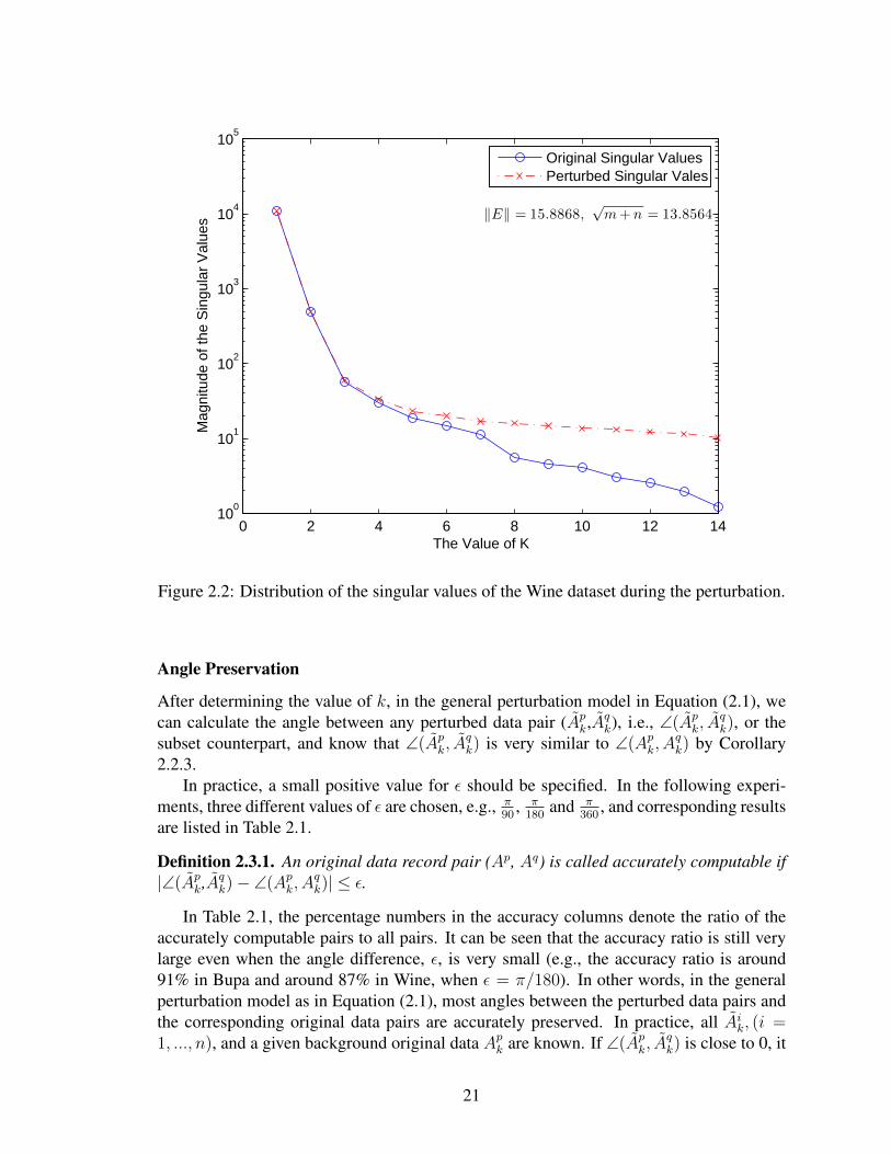
Based on Figures 2.1 and 2.2, it is clear that the singular values (eigenvalues) of theperturbed datasets are very close to those of the original datasets. In Figure 2.1, the first 6perturbed singular values are almost the same as those of the original ones, (the two linesoverlap at the beginning, and they diverge starting at the 6-th point). In Figure 2.2, the first4 perturbed singular values are almost identical to the original ones, (they overlap from thefirst point to the 4-th point). The difference between the last perturbed singular value andthe corresponding original one is still very small, (note that the y-axes of these figures are ina logarithmic scale). Therefore, the perturbed singular values σi can be used to approximatethe first few original singular values (σi ≈ σi). From the two figure legends, there are no bigdifferences between ‖E‖ and

√m+ n, given the comparatively large singular values. For

example, for the Bupa dataset, ‖E‖ = 20.3467 and√m+ n = 18.7083, their difference

is much smaller than the singular values, σ1 = 2385.5 and σ∗1 = 2388.2, (σ4 = 263.6 andσ∗4 = 264.6).

20

0 2 4 6 8 10 12 1410

0

101

102

103

104

105

Mag

nitu

de o

f the

Sin

gula

r V

alue

s

The Value of K

‖E‖ = 15.8868,√m+ n = 13.8564

Original Singular ValuesPerturbed Singular Vales

Figure 2.2: Distribution of the singular values of the Wine dataset during the perturbation.

Angle Preservation

After determining the value of k, in the general perturbation model in Equation (2.1), wecan calculate the angle between any perturbed data pair (Apk,A

qk), i.e., ∠(Apk, A

qk), or the

subset counterpart, and know that ∠(Apk, Aqk) is very similar to ∠(Apk, A

qk) by Corollary

2.2.3.In practice, a small positive value for ε should be specified. In the following experi-

ments, three different values of ε are chosen, e.g., π90

, π180

and π360

, and corresponding resultsare listed in Table 2.1.

Definition 2.3.1. An original data record pair (Ap, Aq) is called accurately computable if|∠(Apk,Aqk)− ∠(Apk, A

qk)| ≤ ε.

In Table 2.1, the percentage numbers in the accuracy columns denote the ratio of theaccurately computable pairs to all pairs. It can be seen that the accuracy ratio is still verylarge even when the angle difference, ε, is very small (e.g., the accuracy ratio is around91% in Bupa and around 87% in Wine, when ε = π/180). In other words, in the generalperturbation model as in Equation (2.1), most angles between the perturbed data pairs andthe corresponding original data pairs are accurately preserved. In practice, all Aik, (i =1, ..., n), and a given background original data Apk are known. If ∠(Apk, A

qk) is close to 0, it

21

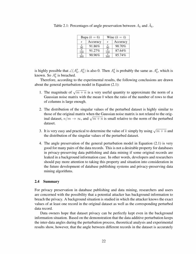
Table 2.1: Percentages of angle preservation between Ak and Ak.

Bupa (k = 6) Wine (k = 4)ε Accuracy ε Accuracyπ90 91.86% π

90 90.70%π

180 91.27% π180 87.64%

π360 90.96% π

360 85.74%

is highly possible that ∠(Apk, Aqk) is also 0. Then Aqk is probably the same as Apk, which is

known. So Aqk is breached.Therefore, according to the experimental results, the following conclusions are drawn

about the general perturbation model in Equation (2.1):

1. The magnitude of√m+ n is a very useful quantity to approximate the norm of a

Gaussian noise matrix with the mean 0 when the ratio of the number of rows to thatof columns is large enough.

2. The distribution of the singular values of the perturbed dataset is highly similar tothose of the original matrix when the Gaussian noise matrix is not related to the orig-inal dataset, n/m → ∞, and

√m+ n is small relative to the norm of the perturbed

dataset.

3. It is very easy and practical to determine the value of k simply by using√m+ n and

the distribution of the singular values of the perturbed dataset.

4. The angle preservation of the general perturbation model in Equation (2.1) is verygood for many pairs of the data records. This is not a desirable property for databasesin privacy-preserving data publishing and data mining if some original records areleaked in a background information case. In other words, developers and researchersshould pay more attention to taking this property and situation into consideration inthe future development of database publishing systems and privacy-preserving datamining algorithms.

2.4 Summary

For privacy preservation in database publishing and data mining, researchers and usersare concerned with the possibility that a potential attacker has background information tobreach the privacy. A background situation is studied in which the attacker knows the exactvalues of at least one record in the original dataset as well as the corresponding perturbeddata record.

Data owners hope that dataset privacy can be perfectly kept even in the backgroundinformation situation. Based on the demonstration that the data additive perturbation keepsthe inter-data angles during the perturbation process, theoretical analysis and experimentalresults show, however, that the angle between different records in the dataset is accurately

22

preserved during the perturbation in the general data perturbation model. Moreover, inthis model, the angle is not only preserved in the original space, but also in the subsetspaces. Obviously, this is extremely undesirable for the privacy protection of databases.For example, if the attacker discovers that one perturbed record (or its subsets) and theperturbed background record (or its corresponding subsets) are similar, through theoreticalanalysis, it is highly possible that the attacker will find that the two records (or their subsets)in the original dataset are similar or even identical. In addition, if the attacker knows manyoriginal data records and the corresponding perturbed version whose number is not lessthan the number of the data’s features, almost all original data records are susceptible tothis data privacy breach analysis.

Copyright c© Lian Liu, 2015.

23

Chapter 3 Wavelet-Based Data Perturbation for Numerical Matrices

To overcome drawbacks of potential breach possibilities of general data noise addition/multiplicationmodel for privacy preservation, a class of novel privacy-preserving data distortion methodsis presented in collaborative analysis situations based on wavelet transformation, whichprovides an effective and efficient balance between data utilities and privacy protectionbeyond its fast run time. A multi-basis wavelet data distortion strategy is given for bet-ter privacy preserving in these situations. Through experiments on real-life datasets, it isconcluded that the multi-basis wavelet data distortion method is a very promising privacy-preserving technique.

Moreover, a privacy-preserving strategy based on wavelet perturbation will be intro-duced to keep the data privacy and data statistical properties and data mining utilities atthe same time. Although some privacy-preserving data perturbation strategies can keepvery good data mining utilities while preserving certain privacy, data statistics are usuallynot included in the consideration of these techniques. For certain applications, it is neces-sary to keep statistical properties so that perturbed data can be used for statistical analysisin addition to the data mining analysis. Hence, a privacy-preserving method is presentedbased on wavelet transformation and normalization to maintain data mining utilities andstatistical properties in addition to the data privacy protection.

3.1 Background and Contributions

In commercial data analysis fields, in order to maximize business profit return and toprovide better customer services, different business organizations may reach a multipartyagreement that each party is willing to share its own commercial data with others. In suchcases, multiparty data mining models are developed based on accurate collaborative dataanalysis. At the same time, taking concrete steps is necessary to ensure that certain privateinformation in each owner’s data is not disclosed to the other parties.

Suppose two scenarios where different companies can share their data. The first oneis referred to as vertically collaborative analysis [159] in which the databases of differentcompanies have exactly the same customer set but the attribute sets of the dataset are differ-ent. The second one is called horizontally collaborative analysis [114] where the attributeset of the multiparty database is the same but companies target at different customer sets. Inboth scenarios, the collaborative analysis is considered as an essential approach to gainingmore comprehensive knowledge from the combined databases.

In the collaborative analysis cases, especially in real-time situations, the time cost is asensitive factor. The wavelet-based transformation is very promising among many method-ologies in terms of the run time complexity, only O(t) (t is the maximum level number ofwavelet decompositions).

Therefore, a class of novel privacy-preserving collaborative analysis methods is devel-oped based on wavelet distortion, suppression and reconstruction (transformation back)strategies with the intention to keep the dimensions of the original and distorted datasets.

Major contributions in this chapter can be summarized as follows:

24

1. Discrete Wavelet Transformation (DWT) and Inverse Discrete Wavelet Transforma-tion (IDWT) are proposed to distort original dataset and the distorted dataset is trans-formed back to the original space to keep the same dimension as the original dataset.Clearly, the purpose of keeping dimension is to facilitate collaborative analysis in thetwo cases.

2. It is discovered that the classification analysis results of the distorted data using onlysingle basis wavelet and the partitioned distorted data using multi-basis wavelet areas good as that of the original one.

3. Based on normalization, experimental results demonstrate that both data privacy andbasic statistical properties can be kept at the same time.

3.2 Algorithms

In this section, the detailed procedures of the privacy-preserving data distortion methodare given based on wavelet transformation for collaborative analysis which can achieve adesirable balance between accurate data utilities and good privacy protection.

The matrix representation (vector-space format) is one of the most popular ways toencode the object-attribute relationships in many real-life datasets. In this chapter, the ma-trix representation (vector-space format) is chosen in which a 2-dimensional (2D) matrixis used to store the dataset in which each row of the matrix stands for an individual objectand each column represents a particular attribute of these objects. Apparently, in this ma-trix, the privacy is a set of all confidential attributes represented by columns and all secretobjects represented by rows. In such a matrix, it is assumed that every element is fixed,discrete, and numerical. Any missing element is not allowed.

Wavelet Decomposition

In mathematical terms, a discrete wavelet transformation (DWT) is a wavelet transforma-tion for which the input discrete samples (x, whose length is 2l, l > 0) are divided intoapproximation coefficients (ylow) and detail coefficients (yhigh) which correspond to thelow frequency and high frequency decompositions of the original samples, respectively.Such wavelet decomposition process is applied recursively with high (h) and low passingfilters (g) on the approximation coefficients of the previous level and then down-sampledas follows.

ylow[l] =∞∑

k=−∞

x[k]g[2l − k]

yhigh[l] =∞∑

k=−∞

x[k]h[2l − k]

Although the standard 2D wavelet decomposition requires the matrix to be representedin 2a ∗ 2b dimensions, where a and b are two integers, it can still deal with matrices of anydimension size. For any 2a∗2b dimension matrix, the DWT decomposition can process and

25

downsample all columns through the standard DWT filters, but the rows may not be suffi-ciently decomposed (for simplicity, it is assumed that a > b). However, in data distortionapplications, that does not matter because it can still suppress the entire detail coefficientsand then reconstruct them and the approximation coefficients, to be introduced in the nextsection, to successfully distort the whole original data if N is large enough (N will bedefined in the next paragraph).

Thus, the maximum number of decomposition levels, N , of a data matrix of any di-mension a ∗ b is defined as: N = dlog2 min(a, b)e.

Coefficient Suppression and Wavelet Reconstruction

Although the original matrix could be replaced by the approximation coefficient matrixas the analysis target dataset, the dimension of the approximation coefficient matrix isdownsized. The strategy proposed by Bapna and Gangopadhyay [14] will further removesome columns of the transformed data deemed as “less important”. So there may be aproblem to use the transformed data in the multiparty collaborative analysis situations,which require the dimensions of the individual datasets to match each other to facilitateanalysis with respect to the corresponding object set or the corresponding attribute set.One way of maintaining dimensions of the dataset matrices is to transform the individualdataset matrices back to the original spaces and to reconstruct the original matrix formats.For the privacy-preserving purpose, data is needed to be distorted when the data entries aretransformed back to the original space.

Therefore, the detail coefficients are suppressed to reduce the high frequency ”noise”which is hidden among the original data entries. The proposed suppression procedure is:

yhigh[i] =

0 if |yhigh[i]| < δ,yhigh[i] + δ if yhigh[i] < 0 and |yhigh[i]| > δ,yhigh[i]− δ if yhigh[i] > 0 and |yhigh[i]| > δ,

where yhigh[i] is the detail coefficient element of the original matrix and δ is a predefinedpositive threshold value. In the experiments, δ=0.5 ∗max(yhigh[i]) is chosen.

With this coefficient suppression process, the inverse discrete wavelet transformation(IDWT) is used on the approximation coefficients and modified detail coefficients to trans-form the data matrix back to the original space to obtain a new data matrix, S∗, which hasthe same dimension as the original data matrix S, but with different attribute values. Thenew data matrix not only preserves the data utilities such as classes and patterns, but alsoprevents intruders from guessing the original attribute values from the distorted matrix.

Multi-Basis Wavelet Transformation

The single basis wavelet transformation distortion algorithm may efficiently prevent thepublic from guessing the true data values. To prevent potential attacker breach exploitationon the simple single basis wavelet distortion, a multi-basis wavelet data distortion strategyis proposed for better privacy preserving in these situations.

Generally speaking, the data matrix can be partitioned in any way, vertically or hor-izontally into any number of submatrices. Since the possibility of guessing the correct

26

matrix partition, the possibility of guessing the correct choice of a particular basis waveletfor a particular submatrix, and the possibility of guessing a particular threshold value for aparticular row or column of a particular submatrix are very remote, the use of multi-basiswavelet and multiple threshold values for data distortion can be very difficult to breach.

3.3 Normalization

After the pre-perturbation process using the above techniques, the following normalizationprocess can be performed in order to keep the same mean value and the standard deviationvalue as the original matrix on every attribute as follows:

A∗∗i,j = (A∗i,j +σ1j

σj∗ µj − µ∗j) ∗

σjσ∗j

i = 1, ..., n, j = 1, ...,m, (3.1)

where A is the n ∗m original matrix, A∗ is the perturbed A∗i,j is the element of A∗ in thei-th row and j-th column. Let µj and µ∗j be the mean values of the j-th column of A andA∗, respectively, and σj and σ∗j be the standard deviation values of A and A∗, respectively.In detail,

µ∗j =1

n∗

n∑i=1

A∗i,j

µj =1

n∗

n∑i=1

Ai,j

σ∗j =

√∑ni=1(A∗i,j − µ∗j)2

n− 1

σj =

√∑ni=1(Ai,j − µj)2

n− 1

After the above normalization process, the matrix A∗∗ is the final version of the per-turbed matrix whose mean values and standard deviation values are the same as those ofthe original matrix A.

Theorem 3.3.1. For the proposed normalization strategy, the following properties hold

(1) µA∗∗j = µj ,

(2) σA∗∗j = σj .

Here µA∗∗j and σA∗∗j are the mean value and standard deviation value of the jth-column ofA∗∗.

27

Proof.

(1).uA∗∗j = E((A∗j +σ∗jσj∗ µj − µ∗j) ∗

σjσ∗j

)

=σjσ∗j∗ [E(A∗j) +

σ∗jσj∗ µj − µ∗j ]

=σjσ∗j∗ (µ∗j +

σ∗jσj∗ µj − µ∗j)

=σjσ∗j∗ (σ∗jσj∗ µj)

= µj,

(2).σA∗∗j = σ((A∗j +σ∗jσj∗ µj − µ∗j) ∗

σjσ∗j

)

=

√∑ni=1(A∗j ∗ σj

σ∗j+ µj − µ∗j ∗ σj

σ∗j− µj)2

n− 1

=

√∑ni=1(A∗j ∗ σj

σ∗j− µ∗j ∗ σj

σ∗j)2

n− 1

=σjσ∗j∗

√∑ni=1(A∗j − µ∗j)2

n− 1

=σjσ∗j∗ σ∗j

= σj,

where E(·) and σ(·) are statistical expectation and deviation operators, respectively.

The following function is defined

f(j) =n∑i=1

(A∗∗i,j − A∗i,j)2 i = 1, ..., n, j = 1, ...,m, (3.2)

as a cost of the perturbation A∗∗ upon A∗ under the constraint of Theorem 3.3.1.

Theorem 3.3.2. The normalization formula (3.1) minimizes the function (3.2) under theconstraint of Theorem 3.3.1. For this method, µj and σj and n are related to the originalmatrix A, so they are all known values. A∗i,j is the element of pre-normalization matrixwhich is known to the data publisher but not to the public. In other words, µj , σj , n andA∗i,j are known, and only A∗∗i,j is variable.

Proof. A Lagrangian Multiplier is constructedL(A∗∗j ) = f(j) + λ1 ∗ (

∑ni=1A

∗∗i,j − n ∗ µj) + λ2 ∗ (

∑ni=1(A∗∗i,j − µj)2 − (n− 1) ∗ (σj)

2).

28

Let L′A∗∗i,j be the first derivative of L(A∗∗j ) with respect to A∗∗i,j .

L′

A∗∗i,j= 2 ∗ (A∗∗i,j − A∗i,j) + λ1 + 2 ∗ λ2 ∗ (A∗∗i,j − µj) = 0,

so A∗∗i,j =2 ∗ λ2 ∗ µj + 2 ∗ A∗i,j − λ1

2 + 2 ∗ λ2

.

According to the following equations

n∑i=1

A∗∗i,j = n ∗ µj,

n∑i=1

(A∗∗i,j − µj)2 = (n− 1) ∗ σj,

the following holds

λ1 = 2 ∗ (µ∗j − µj),

λ2 =σ∗jσj− 1.

So,

L(A∗∗j ) =n∑i=1

(A∗∗i,j − A∗i,j)2

+ 2 ∗ (µ∗j − µj) ∗ (n∑i=1

A∗∗i,j − n ∗ µj)

+ (σ∗jσj− 1) ∗ (

n∑i=1

(A∗∗i,j − µj)2

− (n− 1) ∗ (σj)2,

dL = 2 ∗n∑i=1

(A∗∗i,j − A∗i,j)dA∗∗i,j

− 2 ∗ (µ∗j − µj) ∗n∑i=1

dA∗∗i,j

+ 2 ∗ (σ∗jσj− 1) ∗

n∑i=1

(A∗∗i,j − µj)dA∗∗i,j,

d2L = 2 ∗ d2A∗∗i,j

+ 2 ∗ (σ∗jσj− 1) ∗

n∑i=1

(A∗∗i,j − µj) ∗ d2A∗∗i,j

>= 2 ∗ σ∗j

σj∗ d2A∗∗i,j > 0.

29

Hence, dL and dA∗∗i,j are the first derivative of L and A∗∗i,j , and d2L is the second derivativeof L. So, the function (3.2) is minimized under the constraint of Theorem 3.3.1 with theformula (3.1).

3.4 Experimental Results

Data Privacy Measures

The five data distortion privacy measure metrics, VD, RP, RK, CP and CK, are defined in[170], and then in [171], to evaluate the proposed data distortion methods. The objective ofthese measure metrics is to evaluate the possibility of estimating the true values and rangeof the original data from the distorted data [55].

In brief,

V D =||A− A||F||A||F

,

where A is the original dataset and A is the perturbed version of A, and ||A|| is the Frobe-nius norm of the matrix A.

The RP value presents the ratio of the average change of ranks for all attributes to thenumber of total elements of the matrix. Its definition is as follows,

RP =1

m

m∑i=1

(

∑nj=1 |Rankij −Ranki∗j |

n),

where for the n*m dataset A, Rankji denotes the rank in the ascending order of the j-thelement in the attribute i, and Rankj∗i denotes the rank in ascending order of the perturbedversion A.

RK denotes the percentage of elements which keep their ranks of values in each columnafter the distortion.

RK =1

m

m∑i=1

(

∑nj=1RK

ij

n),

where RKij=1 if Rankij=Rank

i∗j , and RKi

j=0 otherwise.CP stands for change of ranks of the average values of the attributes.

CP =

∑mi=1 |RAVi −RAV ∗i |

m,

where RAVi (resp. RAV ∗i ) is the rank in the ascending order of the average value of thei-th attribute at A (resp. A).

CK is defined to evaluate the percentage of the attributes that keep their ranks of averagevalues after the distortion.

CK =

∑mi=1CK

i

m,

30

Table 3.1: Performance comparison of SVD and wavelet transformation on WBC.

Database VD RP RK CP CK Time AccuracyOriginal 96.0%

SVD 0.2080 239.4 0.006358 1.556 0.4444 0.07882 95.9%Wavelet(S) 0.2557 238.6 0.004769 1.333 0.5556 0.03081 96.0%

Wavelet(VP) 0.3526 247.1 0.005564 1.556 0.333 0.06362 95.6%Wavelet(HP) 0.3140 239.1 0.005087 2.000 0.333 0.05153 96.1%

where CKi = 0 if RAVi=RAV ∗i , and CKi=0 otherwise.According to their definitions, it is clear that a larger VD, RP and CP, and a smaller RK

and CK value refers to a better privacy-preserving level.

Distortion Experiments

In the experiment section, two real-life databases are obtained from Machine LearningRepository [10] at the University of California, Irvine (UCI). They are the Wisconsin breastcancer original dataset (WBC) donated by Olvi Mangasarian in which 699 instances with9 features are in 2 classes, and the Wisconsin breast cancer diagnostic database (WDBC)donated by Nick Street where 599 examples with 30 features also belong to 2 classes. Theattributes of the two databases only have numerical values and no missing value. (In theoriginal WBC database, there are a few missing values in the sixth column. These missingvalues are replaced by 1 if the object belongs to the malignant class and 2 if the object is inthe benign class, according to the standard classification provided by the UCI Repository.)

Tables 3.1 and 3.2 demonstrate the privacy-preserving distortion experimental results.In the experiments, the SVD-based data distortion method is chosen for comparison [170,171]. The simplest SVD data distortion method, i.e., no sparsification strategy, is imple-mented. For each database, three wavelet transformations are performed: the single basiswavelet transformation (S), the vertically partitioned multi-basis wavelet transformation(VP), and the horizontally partitioned multi-basis wavelet transformation (HP).

In the SVD data distortion experiment, the reduced rank k is chosen to be 5 in WBCand 15 in WDBC.

For simplicity, in the vertical and horizontal partitions, the original database is onlypartitioned into two submatrices and each submatrix is approximately a half of the originalone in size.

In the single basis wavelet transformation (S) of both Tables 3.1 and 3.2, the Haarbasis wavelet is chosen for decomposition and reconstruction. In the vertically (VP) andhorizontally (HP) partitioned multi-basis wavelet transformations of both Tables 3.1 and3.2, Haar basis wavelet is selected for the first half partition and Daub-4 basis wavelet forthe second half for decomposition and reconstruction.

The time reported is the measure of the summed time in seconds of all transformationsboth in the single basis wavelet and the multi-basis wavelet processes.

31

Table 3.2: Performance comparison between SVD and wavelet transformation on WDBC.

Database VD RP RK CP CK Time AccuracyOriginal 85.4%

SVD 0.000035 121.3 0.3454 0 1.0000 0.13880 85.4%Wavelet(S) 0.000843 165.3 0.1083 4.800 0.4000 0.05166 85.4%

Wavelet(VP) 0.001011 168.6 0.1041 4.733 0.4667 0.09274 85.4%Wavelet(HP) 0.000962 165.5 0.1141 3.267 0.4667 0.08177 85.4%

The results of experiments, especially the run time, are averaged values of five repeatedexperiments, obtained from a Dell desktop workstation with a P4-2.8GHz CPU, 40G hard-disk, and 256MB memory in Matlab 6.5.0.180913a with a Linux operating system. Forthe results reported in Tables 3.1 and 3.2, the support vector machine (SVM light) with afive-fold cross validation [88] is employed as the standard classification tool which is usedto measure the data utility accuracy in the experiments. According to Tables 3.1 and 3.2,the following conclusions can be drawn:

1. The data accuracy level of the wavelet-based distortion methods is as good as that ofthe SVD and the original data.

2. The run time of the wavelet-based distortion methods is faster than that of the SVD-based method even in the multi-basis wavelet transformation. When the size of thedataset is larger, this advantage is more significant.

3. Most of the privacy preservation metrics show that the wavelet-based distortion meth-ods can keep a better privacy level than the standard SVD-based method.

4. In the three wavelet-based distortion methods (S, VP and HP), their analysis accuracyand privacy-preserving and run time performances are similar.

After wavelet-based data perturbation, this chapter normalizes the post-perturbed data.Specially, for SVD and wavelet methods, because the different parameters of such twomethods have a varied influence on the final results, it shows that every final results indifferent parameter conditions. In details, for SVD the k value could be chosen from 1 tothe rank(A)−1, while for wavelet the coefficient suppression percentage is from 10% to90% in Table 3.4.

3.5 Summary

In this chapter, a class of new privacy preserving data distortion methods is proposed basedon wavelet transformation. Through experiments, the wavelet-based data distortion meth-ods, especially the multi-basis wavelet transformation, can effectively and efficiently ren-der a balance between data utilities and data privacy beyond its fast run time in comparisonwith the SVD-based distortion method which has already been demonstrated as a promis-ing privacy preserving data distortion method [170]. Besides, the post-perturbed data can

32

Table 3.3: Different parameter comparison of SVD and wavelet perturbation.

Without Statistics With Statisticsk Accuracy VD Accuracy VD1 96.28% 0.196 96.28% 0.19152 95.71% 0.1909 95.99% 0.19263 95.71% 0.1527 95.42% 0.15634 95.85% 0.1442 95.71% 0.143

SVD 5 95.85% 0.132 95.99% 0.13896 95.85% 0.1254 95.99% 0.12267 95.99% 0.1075 96.14% 0.10768 95.99% 0.0767 96.28% 0.0764

average 95.90% 0.1407 95.98% 0.1411

percentage Accuracy VD Accuracy VD10% 95.99% 0.0341 95.99% 0.025720% 95.99% 0.067 95.99% 0.050730% 95.85% 0.0985 95.85% 0.075140% 95.57% 0.1276 95.57% 0.098850% 95.57% 0.1558 95.71% 0.1232

Wavelet 60% 95.85% 0.1824 95.99% 0.147870% 95.85% 0.2082 96.14% 0.173480% 94.56% 0.2332 95.28% 0.200390% 94.42% 0.2567 94.56% 0.2273

average 95.52% 0.1515 95.68% 0.1247

be normalized to keep the data statistical properties the same as for the original dataset inorder to facilitate statistical analysis.

Copyright c© Lian Liu, 2015.

33

Chapter 4 Privacy Preservation in Social Networks with Sensitive Edge Weights

With the development of social networks, such as Facebook and MySpace, security andprivacy threats arising from social network analysis bring a risk of disclosure of confidentialknowledge when the social network data is shared or made public. In addition to the currentsocial network anonymity de-identification techniques, a business transaction warehouseis essentially a social network, in which weights are attached to network edges that areconsidered to be confidential (e.g., transactions). In such a business transaction socialnetwork, weight can represent the cost of one transaction between two business entities, thephysical distance between two stores, to name a few. Perturbing the weights of some edgesis for preserving data privacy when the network is published, while retaining the shortestpath and the approximate length of the path between some pairs of nodes is required inthe original network. Two privacy-preserving strategies are developed for this application.The first strategy is based on a Gaussian randomization multiplication, the second one is agreedy perturbation algorithm based on graph theory. In particular, the second strategy notonly yields an approximate length of the shortest path while maintaining the shortest pathbetween selected pairs of nodes, but also maximizes privacy preservation of the originalweights. Experimental results are given to support mathematical analysis.

4.1 Background

Due to recent advances in computer and network, gathering and collecting data concerningdifferent individuals and organizations becomes relatively easy. Establishing and research-ing social networks have become a major interest in data mining communities. There area variety of social networks published so far for research purpose, including those for epi-demiologists [142], sociologists [144], zoologists [59], intelligence communities (terrorismnetworks) [15], and much more.

A social network is a special graph structure made of entities and connections betweenthese entities. The entities, or nodes, are abstract representations of either individuals or or-ganizations that are connected by one or more attributes. The connections, or edges, denoterelationships or interactions between these nodes. Connections can be used to represent fi-nancial exchanges, friend relationships, conflict likelihood, web links, sexual relations,disease transmission (epidemiology), etc.

Social networks typically contain a large amount of private information and are goodsources for data analysis and data mining. The need to protect confidential, sensitive,and security information from being disclosed motivates researchers to develop privacy-preserving techniques for social networks. One of the major challenges, therefore, is toapproach an optimal tradeoff between securing the confidential information and maximiz-ing the social network’s utility analysis.

Recent study of privacy preservation in social networks focuses on the de-identificationprocess to protect the privacy of individuals while preserving the patterns between smallcommunities [77, 179, 182]. Such de-identification processes are often helpful when theindividual’s identity is considered to be confidential, such as a patient’s identity.

34

However, the individual identity is not always considered to be confidential. For ex-ample, a recent tool called ArnetMiner [155] has been developed to allow mining the aca-demic research network through a public web portal. Each node of this network representsa researcher. An edge exists between two nodes if the corresponding researchers share aco-authorship. Another feature that is supported by the system is the association searchbetween two researchers, which enumerates all possible topics that connect one researcherto the other and show how closely the two researchers are connected. In this case, sinceall data needed to compute such network are obtained from public web pages or databases,privacy of identity is not a big concern. However, it is important to realize that the networkderived from these public data makes implicit knowledge explicit and more specific, suchas the association between individuals.

Next, another example of weighted social networks is given, which is thoroughly stud-ied in [83]. The social network represents an automotive business network between Japanesecorporations and American suppliers in North America. The background behind this exam-ple is that many Japanese automotive companies have already taken roots in North Amer-ica, and American suppliers would seek access to such a profitable subcontract market.On one hand, the existence of a long-term and loyal connection between Japanese first-tiersuppliers and auto makers plays a key role in making decisions. So these preferences surelyprevent American suppliers from obtaining contracts easily. On the other hand, since mostfirst-tier suppliers are sensitive to importing cost and have U.S. political pressure to avoidmass outsourcing, they prefer to collaborate with the qualified local American suppliers.Therefore, it is practical and economical to become a subcontractor of these lower-levelsuppliers. For every potential American supply contractor, it is desirable to obtain a com-prehensive business network that can guide them in finding the most economical businesspath.

However, due to the fierce competition between suppliers, managers may not be willingto disclose the true transaction expenses to their adversaries. Otherwise, their adversariescould probably reduce the quotation below the price obtained in a secret bidding compe-tition. Hence, suppliers would like to preserve their transaction expenses (edge weights)before the business network is published. At the same time, some global and local utili-ties of the social networks, such as the optimal supply chains (the lowest cost path betweencompanies) and the corresponding lengths, are probably desired to be maintained for futureanalysis.

In this chapter, the focus is on publishing a social network which maintains the utilityof the shortest paths while perturbing the actual weight between a pair of entities. Theedge between two nodes is often associated with a quantitative weight that reflects theaffinity between the two entities. The weighted graph allows deeper understanding aboutrelationships between entities within the network. The shortest path between a pair ofnodes is a path such that the sum of the weights of its constituent edges is to be minimum.The shortest path is a major data utility which has applications in different fields.

So each node in this business graph represents a company or a supplier (or an agent),the edge denotes business relationship and the weight of the edge represents the transactionexpenses according to some measures (such as per month, per person or per transaction)between the two entities [175]. As an abstract business network in Figure 4.1, the boldnumbers beside edges are the transaction expenses per month (the unit is million/month).

35

In this business example, for example, Company A wants to purchase some products orservices, in the future, from Company D which cannot directly access each other due tosome trade barriers. Company A needs to choose some trade intermediate suppliers whohave the most competitive path (the shortest path of price) between themselves and Com-pany D (maybe these suppliers need other suppliers to connect Company D). If the weightsof the business social network are perturbed as in Figure 4.2 but the shortest paths (andthe corresponding lengths) are well preserved, Company A may be able to make an in-telligent decision based on this privacy-preserving social network without having to knowconfidential details of the relationship between agents and Company D.

According to the proposed algorithms, the perturbed graph preserves the same shortestpaths and maintains the shortest path lengths close to the true values. Moreover, the totalprivacy of all edge weights is maximized by the methods. Here, the more weight of anedge changes, the more edge’s privacy is preserved. As the example in Figure 4.1, the trueexpense between Agent 2 (or Supplier 2) and Company D is lower than that between Agent3 (or Supplier 3) and Company D, but in the perturbed network as in Figure 4.2, the expensebetween Agent 2 and Company D is higher than that between Agent 3 and Company D. Soin a bidding competition, the business secret between Agent 2 and Company D is blind toAgent 3 (Agent 2’s adversary) even if the perturbed business network is published. Aftera series of perturbations, the final perturbed version is in Figure 4.2. The shortest pathbetween Company A and Company D is the same as the original one and the correspondingperturbed length is close to the original one.

Figure 4.1: Original business network. All nodes in this figure represent either a companyor an agent (supplier) and the edge means a business connection between the two entities.The weight of each edge denotes the transaction expense of the corresponding businessconnection.

To utilize the privacy-preserving social network analysis, each people (or organization)has a local (private) weighted graph before perturbation. The process of information shar-

36

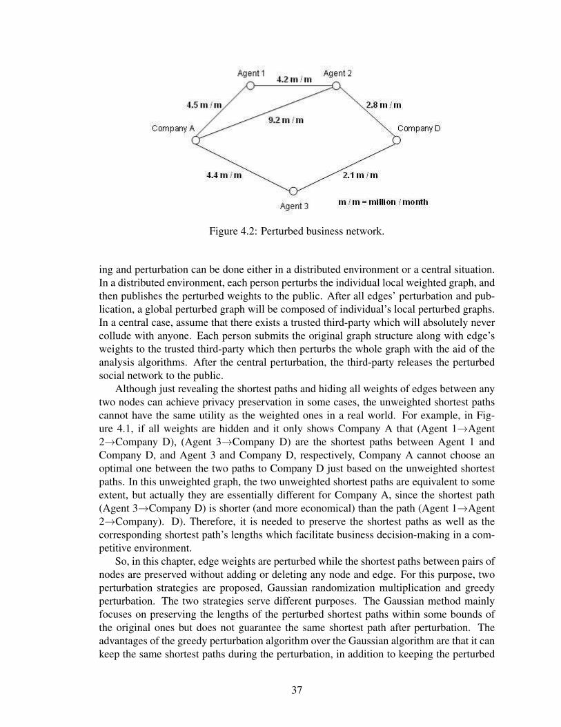
Figure 4.2: Perturbed business network.

ing and perturbation can be done either in a distributed environment or a central situation.In a distributed environment, each person perturbs the individual local weighted graph, andthen publishes the perturbed weights to the public. After all edges’ perturbation and pub-lication, a global perturbed graph will be composed of individual’s local perturbed graphs.In a central case, assume that there exists a trusted third-party which will absolutely nevercollude with anyone. Each person submits the original graph structure along with edge’sweights to the trusted third-party which then perturbs the whole graph with the aid of theanalysis algorithms. After the central perturbation, the third-party releases the perturbedsocial network to the public.

Although just revealing the shortest paths and hiding all weights of edges between anytwo nodes can achieve privacy preservation in some cases, the unweighted shortest pathscannot have the same utility as the weighted ones in a real world. For example, in Fig-ure 4.1, if all weights are hidden and it only shows Company A that (Agent 1→Agent2→Company D), (Agent 3→Company D) are the shortest paths between Agent 1 andCompany D, and Agent 3 and Company D, respectively, Company A cannot choose anoptimal one between the two paths to Company D just based on the unweighted shortestpaths. In this unweighted graph, the two unweighted shortest paths are equivalent to someextent, but actually they are essentially different for Company A, since the shortest path(Agent 3→Company D) is shorter (and more economical) than the path (Agent 1→Agent2→Company). D). Therefore, it is needed to preserve the shortest paths as well as thecorresponding shortest path’s lengths which facilitate business decision-making in a com-petitive environment.

So, in this chapter, edge weights are perturbed while the shortest paths between pairs ofnodes are preserved without adding or deleting any node and edge. For this purpose, twoperturbation strategies are proposed, Gaussian randomization multiplication and greedyperturbation. The two strategies serve different purposes. The Gaussian method mainlyfocuses on preserving the lengths of the perturbed shortest paths within some bounds ofthe original ones but does not guarantee the same shortest path after perturbation. Theadvantages of the greedy perturbation algorithm over the Gaussian algorithm are that it cankeep the same shortest paths during the perturbation, in addition to keeping the perturbed

37

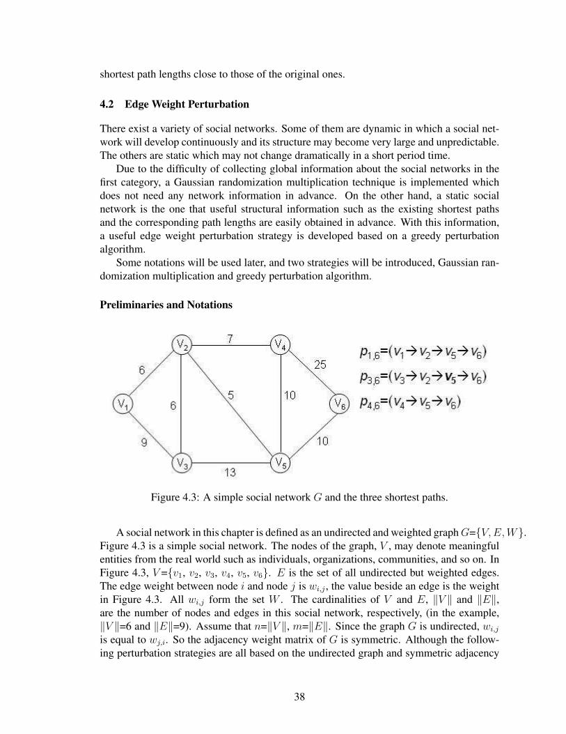
shortest path lengths close to those of the original ones.

4.2 Edge Weight Perturbation

There exist a variety of social networks. Some of them are dynamic in which a social net-work will develop continuously and its structure may become very large and unpredictable.The others are static which may not change dramatically in a short period time.

Due to the difficulty of collecting global information about the social networks in thefirst category, a Gaussian randomization multiplication technique is implemented whichdoes not need any network information in advance. On the other hand, a static socialnetwork is the one that useful structural information such as the existing shortest pathsand the corresponding path lengths are easily obtained in advance. With this information,a useful edge weight perturbation strategy is developed based on a greedy perturbationalgorithm.

Some notations will be used later, and two strategies will be introduced, Gaussian ran-domization multiplication and greedy perturbation algorithm.

Preliminaries and Notations

Figure 4.3: A simple social network G and the three shortest paths.

A social network in this chapter is defined as an undirected and weighted graphG={V,E,W}.Figure 4.3 is a simple social network. The nodes of the graph, V , may denote meaningfulentities from the real world such as individuals, organizations, communities, and so on. InFigure 4.3, V ={v1, v2, v3, v4, v5, v6}. E is the set of all undirected but weighted edges.The edge weight between node i and node j is wi,j , the value beside an edge is the weightin Figure 4.3. All wi,j form the set W . The cardinalities of V and E, ‖V ‖ and ‖E‖,are the number of nodes and edges in this social network, respectively, (in the example,‖V ‖=6 and ‖E‖=9). Assume that n=‖V ‖, m=‖E‖. Since the graph G is undirected, wi,jis equal to wj,i. So the adjacency weight matrix of G is symmetric. Although the follow-ing perturbation strategies are all based on the undirected graph and symmetric adjacency

38

weight matrix, they can be easily modified for the directed graphs and the correspondingnonsymmetric adjacency weight matrices.

Let w∗i,j be the perturbed weight of the edge between node i and node j, di,j and d∗i,j bethe shortest path lengths between node i and node j before and after a perturbation strategy,respectively, pi,j and p∗i,j be the shortest paths between node i and node j before and aftera perturbation strategy, respectively.

Distributed Perturbation by Gaussian Randomization Multiplication

In this section, some preliminaries and the intuition behind edge weight perturbation strat-egy are given in a social network represented as an undirected but weighted graph withoutloops and multiedges.

The basic idea behind this algorithm is that every two linked nodes cooperate withthe generation of a random number which is consistent with a Gaussian distribution. Theweight of the edge connecting these two entities is multiplied by the random number andthe individual perturbed weight is released to the public. Because each edge’s randomnumber and the edge’s perturbation process is only related to these two linked entities, therandom number generation and weight perturbation have nothing to do with other edges. Inother words, the perturbation of all edge’s weights can be done in a distributed environment.The maximum increment or decrement of each weight is only dependent on the parametersof this distribution. So the shortest paths and the corresponding lengths will probably bepreserved if the parameters of the Gaussian distribution are chosen appropriately. Assumethat the parameters of the Gaussian distribution are predefined and globally known.

Proposition 4.2.1. There does not exist a perturbation schema such that every edge weightis perturbed but the shortest paths and the corresponding lengths between every pair ofnodes are preserved.

Proof. By contradiction.Let ei,k1 , ek1,k2 , ..., ekh−1,kh , ekh,j be the shortest path between node i and node j, theircorresponding weights are wi,k1 , wk1,k2 , ..., wkh−1,kh , wkh,j . Suppose that there is a per-fect perturbation strategy which perturbs each edge weight but preserves every node pair’sshortest path length. Obviously, after the perturbation, the path e∗i,k1 , e∗k1,k2 , ..., e∗kh−1,khis the shortest path between nodes i and kh which can be easily proved by contradiction(subpaths of the shortest paths are the shortest paths, see pp. 519 of [36]), and di,kh=d∗i,kh .The following holds

d∗i,j = d∗i,kh + w∗kh,j= di,kh + w∗kh,j6= di,kh + wkh,j, (∵ wkh,j 6= w∗kh,j)

= di,j

Hence, the assumption at the beginning of the proof is incorrect. Namely, there does notexist such a perfect perturbation schema.

39

Gaussian randomization multiplication strategy. Assume that W is an n ∗ n matrixwhose entries are either weights if two nodes have a link or ∞ otherwise. W is calledthe adjacency weight matrix of the graph G. W ∗ is the perturbed adjacency weight matrixwith the same dimension after this schema. N(0,σ2) stands for an n∗n symmetric Gaussiannoise matrix with the mean 0 and the standard deviation σ. Define the perturbed weight ofeach edge as

w∗i,j = wi,j(1− xi,j), i, j = 1, ..., n.

Here xi,j is a randomly generated number from the Gaussian distribution N(0, σ2).If node vi has a connection with vj , then vi generates a random number, x1

i,j , from theGaussian distribution N(0, σ2), and vj also generates a random number, x2

i,j , from thesame distribution. xi,j is the averaged value between x1

i,j and x2i,j . The Gaussian-perturbed

version of the graph G in Figure 4.3 is shown in Figure 4.4. Here, the symmetric Gaussiannoise matrix is generated from N(0, 0.152) (σ=0.15).

Note that the above multiplication is based on undirected graphs. If the weight mul-tiplication is extended to directed graph cases, the cooperation of generating xi,j is notnecessary. Instead, if node vi has a directed edge from node i to node j, then node i candirectly generate a random number xi,j from the Gaussian distribution without the cooper-ation with node j. Other procedures are the same as the above undirected graph case.

The reasons why the Gaussian randomization multiplication strategy is chosen are asfollows. 1). It is straightforward to implement in practice. 2). Due to the dynamic evolutionnature of social networks, collecting all global information in advance is very hard or costlyin a huge and dynamic social network. In particular, in an evolutionary environment, somenodes or edges will emerge in the future and be added to the current network, in which thecollection of the current state will probably be totally changed after these insertions. Soit is impossible or useless to collect comprehensive global information at a given time forlater analysis.

The perturbed graph is reconstructed as G∗={V ∗, E∗,W ∗}. It is clear that the aboveGaussian randomization multiplication strategy does not change the structure of the origi-nal graph. Namely, V =V ∗, E=E∗. The only difference between G and G∗ is the weights.

In Figure 4.4, all values of V ∗ and E∗ are the same as those of V and E in Figure 4.3.The major difference between G∗ and G in these figures is the numbers corresponding tothe weights.

For most paths in the network, using Gaussian randomization multiplication will keepa perturbed shortest path length close to the original one within a small range, 2σ, as shownin Theorem 4.2.1.

Theorem 4.2.1. In the Gaussian randomization multiplication strategy, assume the lengthof a path (vi → vk1 → vk2 → ... → vkh → vj) is Li,j (their edges are ei,k1 , ek1,k2 , ...,ekh−1,kh , ekh,j , and their weights are wi,k1 , wk1,k2 , ..., wkh,j). L

∗i,j and w∗i,k1 , w∗k1,k2 , ..., w∗kh,j

are the corresponding perturbed values after the Gaussian algorithm, then

Pr( |L∗i,j − Li,j|

Li,j≤ ζσ

)> erf

(ζ√2

), for different i, j,

where i and j denote the beginning and ending nodes of the path, σ is the standard deviationof the Gaussian distribution and ζ can be any positive integer.

40

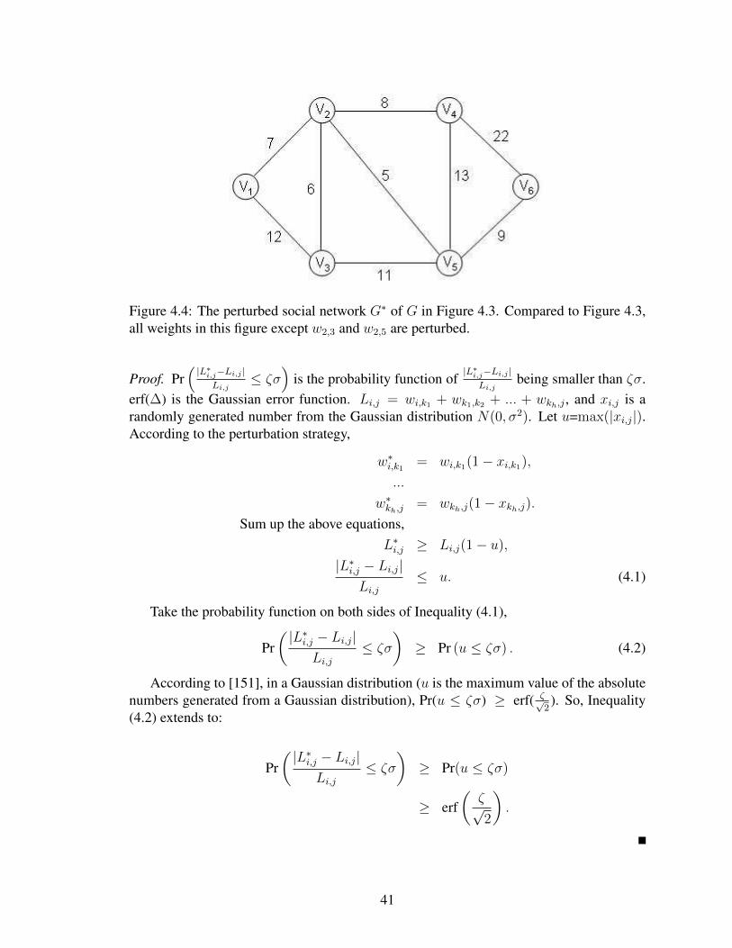
Figure 4.4: The perturbed social network G∗ of G in Figure 4.3. Compared to Figure 4.3,all weights in this figure except w2,3 and w2,5 are perturbed.

Proof. Pr(|L∗i,j−Li,j |

Li,j≤ ζσ

)is the probability function of

|L∗i,j−Li,j |Li,j

being smaller than ζσ.erf(∆) is the Gaussian error function. Li,j = wi,k1 + wk1,k2 + ... + wkh,j , and xi,j is arandomly generated number from the Gaussian distribution N(0, σ2). Let u=max(|xi,j|).According to the perturbation strategy,

w∗i,k1 = wi,k1(1− xi,k1),...

w∗kh,j = wkh,j(1− xkh,j).Sum up the above equations,

L∗i,j ≥ Li,j(1− u),

|L∗i,j − Li,j|Li,j

≤ u. (4.1)

Take the probability function on both sides of Inequality (4.1),

Pr( |L∗i,j − Li,j|

Li,j≤ ζσ

)≥ Pr (u ≤ ζσ) . (4.2)

According to [151], in a Gaussian distribution (u is the maximum value of the absolutenumbers generated from a Gaussian distribution), Pr(u ≤ ζσ) ≥ erf( ζ√

2). So, Inequality

(4.2) extends to:

Pr( |L∗i,j − Li,j|

Li,j≤ ζσ

)≥ Pr(u ≤ ζσ)

≥ erf(ζ√2

).

41

The path in question is not required to be the shortest path, and it could be any pathbetween the two nodes.

From [151], erf( 1√2), erf( 2√

2) and erf( 3√

2) are approximately equal to 0.68, 0.95 and

0.997, respectively. In other words, if the parameter σ is carefully chosen, based on theabove theorem, the weight summations of each path, including the shortest path, can bepreserved as close as possible to those of the original social network while protecting theexact edge weights of the original networks from disclosure.

Comparing Figure 4.3 to Figure 4.4, all perturbed shortest path lengths between everynode pair except for d∗1,3 are in the corresponding range [di,j(1− 2σ), di,j(1 + 2σ)], whereσ=0.15. d1,3 is 9 and d∗1,3 is 12 and the difference is 0.33 which is more than 2σ. In otherwords, in the totally 15 shortest paths (due to the symmetry, pi,j and pj,i are counted onlyonce), the lengths of the 14 perturbed shortest paths are in the range [di,j(1-2σ), di,j(1+2σ)]with the length of just one perturbed shortest path, p∗1,3, being outside the range. The ratioof the perturbed shortest path lengths falling within the range ±2σ is 14/15=93% which isconsistent with mathematical analysis in Theorem 4.2.1.

Corollary 4.2.1. Let di,j be the length of the shortest path between node i and node j.Assume dsecondi,j is the length of the second shortest path between them. Define a ratio

βi,j =dsecondi,j − di,j

di,j.

If βi,j is greater than 2σ, the shortest path is highly possible to be preserved after theGaussian randomization multiplication strategy. Here, σ is the parameter of the Gaussiannoise matrix N(0,σ2).

According to Corollary 4.2.1, in the case of a good choice of σ, for example, σ ∈ [0.1,0.2], Gaussian randomization multiplication strategy preserves not only the very accurateshortest path length between certain pairs, but also exactly the same shortest path afterperturbation strategy.

Comparing Figure 4.3 to Figure 4.4 again, all perturbed shortest paths, except p∗3,5,p∗4,5 and p∗4,6, are identical with the original ones. In this example, all the three shortestpaths have two different paths of an equal length, (p∗3,5=(v3 → v5) or (v3 → v2 → v5),p∗4,5=(v4 → v5) or (v4 → v2 → v5), p∗4,6=(v4 → v6) or (v4 → v5 → v6)), the second of theseis different from the corresponding original ones. Therefore their perturbed shortest pathsare changed even one of their perturbed shortest paths is the same as that of the originalone.

But the Gaussian randomization multiplication strategy cannot guarantee the sameshortest path preservation after perturbation, if βi,j is very small. For example, the originalshortest path length between v3 and v5 in Figure 4.3 is 11 (v3 → v2 → v5) and the originalsecond shortest path length is 13 (v3 → v5). Its ratio β3,5 is (13-11)/11=0.18 which is notgreater than 2σ. According to Corollary 4.2.1, the perturbed shortest path may be changedafter the Gaussian strategy. Actually, in this example, p∗3,5 has two different shortest pathswhich are not considered to be exactly preserved in comparison to the original p3,5 accord-ing to the above statement. By contrast, the original shortest path length between v1 and v6

in Figure 4.3 is 21 (v1 → v2 → v5 → v6) and the original second shortest path length is

42

30 (v1 → v3 → v2 → v5 → v6). So the perturbed shortest path, p∗1,6, is exactly preservedsince the ratio is (30-21)/21=0.43 which is greater than 2σ.

Therefore, another strategy is proposed to ensure that, for certain selected shortestpaths, the perturbation strategy preserves exactly the same shortest paths in any cases in astatic social network in the next section.

Shortest Path Preserving Greedy Perturbation Algorithm

In a static social network, some necessary information about this social network for analy-sis and privacy-preserving purpose is first collected. But a trusted third-party is needed whowill absolutely never collude with any network entities. All social network entities submittheir original graph structures along with the edge’s weights to the third-party. Then allanalysis and perturbation procedures are done by the third-party, and a global perturbedsocial network will be published to the public after the perturbation. Because all analy-sis and perturbation are done by a central third-party, the undirected social network anddirected one have a very similar procedure. In detail, only the directed edges (and thecorresponding weights) and directed paths (and the corresponding lengths) are chosen tobe fed into the following analysis and perturbation in a directed social network. So, thedifference is not distinguished between undirected and directed social networks below.

Before applying perturbation strategy, assume that not all shortest paths of node pairsin a social network are considered to be significant. Actually, in the real world, it is not rea-sonable that all information is considered as confidential. Suppose that only the data ownerhas the right to select which shortest paths should be preserved or which ones should notbe preserved. The tasks are, under data owner’s restrictions, to maximize the preservationof edge weight’s privacy and minimize the difference of the shortest paths and the cor-responding lengths between the original social networks and perturbed ones as much aspossible.

In other words, the assumption that not all shortest paths are confidential keeps theprivate shortest paths (the starting and ending nodes, (s1,s2), in the shortest paths form anode pair set H , see below) and the corresponding lengths as close to the original onesas possible, while ignoring possible changes to other public paths. Let H be the set oftargeted pairs whose shortest paths and the corresponding path lengths should be preservedas much as possible. For example, in the graphG={V,E,W} in Figure 4.3, letH be {(1,6),(4,6), (3,6)}. In a real social network, some of the shortest paths are just one-edge lengthpaths, e.g., p1,3=e1,3, but it is assumed that these shortest paths are not included in H . Inthis case, the greedy perturbation algorithm aims to keep the exact shortest paths and thecorresponding close path lengths between v1 and v6, v4 and v6, v3 and v6, respectively.

Then, in a social network G={V,E,W} (‖V ‖=n), the shortest path list set P and thecorresponding length n ∗ n matrix D are generated. In P , each entry ps1,s2 is a linkedlist representing the shortest path between s1 and s2, (i.e., s1 and s2 are the beginning andending nodes of the shortest path, respectively). For example, p1,6=(v1 → v2 → v5 → v6),the shortest path p1,6 successively passes through v1, v2, v5 and v6. In the matrix D, eachds1,s2 is the length of the shortest path connecting s1 and s2. In the following contents, allnode pairs (s1, s2) of ps1,s2 and ds1,s2 are in the set H unless otherwise stated explicitly.

43

So, the goal is to generate a perturbed graph G∗={V ∗, E∗,W ∗} which satisfies theconditions in Figure 4.5.

1. V ∗ = V and E∗ = E,

2. maximize the number of w∗i,j such that

w∗i,j 6= wi,j,

3. d∗s1,s2 ≈ ds1,s2, for every (s1,s2) in H,

4. p∗s1,s2 = ps1,s2, for every (s1,s2) in H.

Here, s1 and s2 are the beginning and

ending nodes of the shortest paths in H,

respectively.

Figure 4.5: The formulization of perturbation purposes.

Based on the combination of the above conditions and the collected information, likeP and D, all edges in G are divided into three different categories as in Figure 4.6 basedon their involvement in the shortest paths to be preserved.

Figure 4.6: Three different categories of edges. The red bold-faced edges are partially-visited edges, the black thin edges are non-visited ones, and the blue dashed edge is theall-visited edge.

Definition 4.2.1. An edge ei,j is a non-visited edge, if ei,j /∈ ps1,s2 for every (s1, s2) ∈ H .In other words, none of the shortest path in P passes through the edge ei,j .

In Figure 4.6, all black thin edges such as edges e1,3, e2,4, e4,6 and e3,5 are non-visitededges, because the shortest paths of all three targeted pairs inH={(1,6), (4,6), (3,6)} do notpass through these edges. In practice, empirically, the non-visited edges are the majorityof edges in a social network.

Definition 4.2.2. An edge ei,j is called an all-visited edge, if ei,j ∈ ps1,s2 for every (s1, s2)∈ H , i.e., all the shortest paths in H pass through the edge ei,j .

44

In Figure 4.6, the blue dashed edge e5,6 is the all-visited edge since the shortest pathsp1,6, p4,6 and p3,6 in H all go through the edge e5,6. Typically, the all-visited edges are veryrare in a real social network.

Definition 4.2.3. An edge ei,j is a partially-visited edge, if ∃ (s1,s2) ∈ H and ∃ (s3,s4) ∈H such that ei,j ∈ ps1,s2 , but ei,j /∈ ps3,s4 . In this case, only some of the shortest paths passthrough this edge while this edge does not appear in other the shortest paths.

The red bold-faced edges in Figure 4.6 are the partially-visited edges. For example, e2,5

is a partially-visited edge since the shortest paths p1,6 and p3,6 pass through the edge e2,5,but p4,6 does not go through it.

Each edge is perturbed in the graph by four different schemes according to these threedifferent categories.

Proposition 4.2.2. If a non-visited edge ei,j increases its weight by any positive value t(the new perturbed weight is w∗i,j = wi,j + t), all ds1,s2 and ps1,s2 in H will not be changed,i.e., d∗s1,s2 = ds1,s2 and p∗s1,s2 = ps1,s2 .

Because nobody in H passes any non-visited edge, increasing the weights of non-visited edges to any value will not change the shortest paths and the corresponding lengthsin H .

Proposition 4.2.3. If an all-visited edge ei,j decreases its weight to any positive value (i.e.,w∗i,j = wi,j−t and w∗i,j > 0), all ps1,s2 inH will not be affected, but ds1,s2 will be decreased.Actually, p∗s1,s2=ps1,s2 and d∗s1,s2 = ds1,s2 − t.

Figure 4.7: Perturbation on the non-visited and all-visited edges.

45

As in the social network shown in Figure 4.3, the non-visited and all-visited edges areperturbed as in Figure 4.7. The weights of the non-visited edges e1,3, e2,4 and e4,6 areincreased, and the weight of the all-visited edge e5,6 is decreased.

In a social network, partially-visited edges are prevalent which are major perturbationtargets. To minimize the difference between the length of the original shortest path and thatof the corresponding perturbed shortest path, two perturbation schemes are developed onpartially-visited edges. If the current length of the perturbed shortest path is bigger than theoriginal one, the weight of one edge in this path can be decreased. Otherwise, its weight isincreased. So increasing and decreasing are two alternate choices to keep the length of theperturbed shortest path close to the original one.

Proposition 4.2.4. If a partially-visited edge ei,j increases its weight by t (the new per-turbed weight is w∗i,j = wi,j + t) and t satisfies the following condition:

0 < t < min{d−s1,s2 − ds1,s2 |for all ps1,s2 such that ei,j ∈ ps1,s2},

all p∗s1,s2 are not changed and d∗s1,s2 (the edge ei,j is in ps1,s2) will become larger, (p∗s1,s2=ps1,s2and d∗s1,s2 = ds1,s2 + t), where d−s1,s2 is the length of the conditional shortest path betweennode s1 and node s2 in a graphG−={V,E−{ei,j, ej,i},W −{wi,j, wj,i}}. G− is the graphin which only the edges ei,j and ej,i and the corresponding weights from G are deleted. Foreach node pair (s1, s2), ds1,s2 ≤ d−s1,s2 .

Figure 4.8: Increasing the weight of the partially-visited edge e2,5.

An example of increasing the weight of the partially-visited edge e2,5 is shown in Figure4.8. The shortest paths of two targeted pairs in H , p1,6 and p3,6, pass through the edge e2,5,but the shortest length path p4,6 does not go through it. Increasing w2,5 will probably affect

46

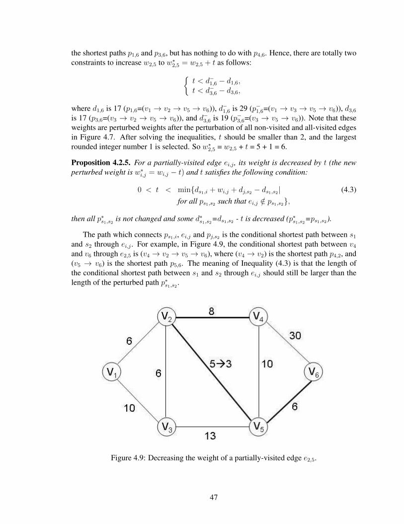
the shortest paths p1,6 and p3,6, but has nothing to do with p4,6. Hence, there are totally twoconstraints to increase w2,5 to w∗2,5 = w2,5 + t as follows:{

t < d−1,6 − d1,6,t < d−3,6 − d3,6,

where d1,6 is 17 (p1,6=(v1 → v2 → v5 → v6)), d−1,6 is 29 (p−1,6=(v1 → v3 → v5 → v6)), d3,6

is 17 (p3,6=(v3 → v2 → v5 → v6)), and d−3,6 is 19 (p−3,6=(v3 → v5 → v6)). Note that theseweights are perturbed weights after the perturbation of all non-visited and all-visited edgesin Figure 4.7. After solving the inequalities, t should be smaller than 2, and the largestrounded integer number 1 is selected. So w∗2,5 = w2,5 + t = 5 + 1 = 6.

Proposition 4.2.5. For a partially-visited edge ei,j , its weight is decreased by t (the newperturbed weight is w∗i,j = wi,j − t) and t satisfies the following condition:

0 < t < min{ds1,i + wi,j + dj,s2 − ds1,s2| (4.3)for all ps1,s2 such that ei,j /∈ ps1,s2},

then all p∗s1,s2 is not changed and some d∗s1,s2=ds1,s2 - t is decreased (p∗s1,s2=ps1,s2).

The path which connects ps1,i, ei,j and pj,s2 is the conditional shortest path between s1

and s2 through ei,j . For example, in Figure 4.9, the conditional shortest path between v4

and v6 through e2,5 is (v4 → v2 → v5 → v6), where (v4 → v2) is the shortest path p4,2, and(v5 → v6) is the shortest path p5,6. The meaning of Inequality (4.3) is that the length ofthe conditional shortest path between s1 and s2 through ei,j should still be larger than thelength of the perturbed path p∗s1,s2 .

Figure 4.9: Decreasing the weight of a partially-visited edge e2,5.

47

An example of decreasing the weight of the partially-visited edge e2,5 is depicted inFigure 4.9. The shortest paths of two targeted pairs in H , p1,6 and p3,6, pass through theedge e2,5, but the shortest length path p4,6 does not go through it. Decreasing w2,5 will notaffect the shortest paths p1,6 and p3,6, but has something to do with p4,6. Hence, there isonly one constraint to decrease w2,5 to w∗2,5 = w2,5 − t as follows:

d4,2 + (w2,5 − t) + d5,6 > d4,6 ⇒ t < d4,2 + w2,5 + d5,6 − d4,6,

where d4,2 is 8 (p4,2=(v4 → v2)), d5,6 is 6 (p5,6=(v5 → v6)), and d4,6 is 16 (p4,6=(v4 →v5 → v6)). After the inequality is solved, t should be smaller than 3, and the largestrounded integer number 2 will be selected. So w∗2,5 = w2,5 - t = 5 - 2 = 3.

Algorithm

Summing up the aforementioned propositions briefly, a practical greedy perturbation pro-cess is as follows (the pseudocode is in Algorithm 1). Based on the original adjacencyweight matrix W , it first generates the shortest paths P and the corresponding lengths Dby Floyd-Warshall algorithm [36] (see Line 1 of Algorithm 1). Then each edge ei,j in Eis determined as in one of the three categories: non-visited, all-visited or partially-visited.The non-visited edges and all-visited edges are perturbed based on Proposition 4.2.2 andProposition 4.2.3 (see Line 2 and Line 3), respectively, before the partially-visited edges,and at the same time, the perturbed adjacency weight matrix W ∗ and the perturbed short-est path length matrix D∗ are updated simultaneously. Then all partially-visited edges aresorted in a descending order based on the number of the shortest paths passing throughthis partially-visited edge. Such all partially-visited edges form a stack PB. From the topto the bottom of this stack PB, it pops out the current top partially-visited edge ei,j , andperturb ei,j only once by either Proposition 4.2.4 or Proposition 4.2.5 based on the verifi-cation whether the number of d∗s1,s2 (ei,j ∈ ps1,s2 and d∗s1,s2 ≤ the original one) is largerthan the number of d∗s1,s2 (ei,j ∈ ps1,s2 and d∗s1,s2 > the original one). If yes, the perturbedweight is increased according to Proposition 4.2.4 (see Lines 8-9). Otherwise, it decreasesthe weight based on Proposition 4.2.5 (see Lines 11-12). Note that an edge popped outfrom PB will never be put back in the stack again. In other words, every partially-visitededge is perturbed only once and the perturbation is a one pass procedure. After perturbingthe weight of any edge, the lengths of the all-pair shortest paths in D∗ will be recalculatedand updated by Floyd-Warshall algorithm. According to these four propositions, all theperturbed shortest paths will not be changed in any case (p∗s1,s2=ps1,s2 , for every (s1, s2)in H according to Propositions 4.2.4 and 4.2.5). The perturbed shortest path lengths willprobably not be the same as the original ones (d∗s1,s2 6= ds1,s2), but the difference is reducedby the alternate choice of either weight increment or decrement.

48

Algorithm 1 Greedy perturbation algorithm.Input: The symmetric adjacency weight matrix W of an original graph G and H (the set

of selected shortest paths to be preserved).Output: The symmetric adjacency weight matrix W ∗ of the corresponding perturbed

graph G∗

1: generate P and D based on W , and assign D to D∗

2: for all non-visited edges ei,j , w∗i,j ⇐ wi,j + r (r is any random positive number), andupdate D∗

3: for all all-visited edges ei,j , w∗i,j ⇐ wi,j - r (r is any random positive number which issmaller than wi,j), and update D∗

4: sort all partially-visited edges in a descending order with respect to the number of theshortest paths which pass through this partially-visited edge. Such all partially-visitededges form a stack PB

5: while PB 6= ∅ do6: pop out the top edge ei,j from PB7: if # of cases where d∗s1,s2 ≤ the original one is larger than # of cases where d∗s1,s2

> the original one then8: generate a random value t given the range determined by Proposition 4.2.49: w∗i,j ⇐ wi,j + t

10: else11: generate a random value t given the range determined by Proposition 4.2.512: w∗i,j ⇐ wi,j - t13: end if14: update D∗

15: end while

49

4.3 Experiments

Databases

In the experiment section, one real database, EIES (Electronic Information Exchange Sys-tem) Acquaintanceship at time 2, is obtained from International Network for Social Net-work Analysis [61].

The EIES data at time 2 were collected by Freeman and Freeman [61]. This datasetwas also discussed in Wasserman and Faust [58]. This is a network of 48 researchers whoparticipated in an early study on the effects of electronic information exchange, a precursorof email communication. The measure of acquaintanceship in this dataset has four levels,from 1 (do not know the other) to 4 (very good friendships). The acquaintanceship in twopeople may not be the same. For example, A thinks B is his/her best friend, but B probablythinks A is a normal friend for him/her. Therefore, the social network in this dataset is di-rected and weighted. If the weight (acquaintanceship in this case) is considered as privacyand need to be protected, the weight should be perturbed. From the individual point ofview, a perturbed weight between two researchers may lose meaning. Based on the globalviewpoint, however, it can still benefit many applications. For example, even all acquain-tanceships between any two researchers are changed, but the shortest paths with respectto the acquaintanceship between two far-away researchers can be kept, which means thatthere are chances of collaboration between the two.

In addition to the EIES database, to test the scalability of the greedy perturbation algo-rithm, a synthetic database is created which consists of 1600 objects and 70% objects areconnected with each other, and the weights of the edges range randomly from 10 to 100.Its corresponding adjacency weight matrix is a 1600*1600 symmetric matrix.

Results with Gaussian Randomization Multiplication Algorithm

Figures 4.10, 4.11 and 4.12 show experimental results with different values of σ in Gaus-sian randomization multiplication. In each figure, the x-axis is the difference between theoriginal ones and the corresponding perturbed ones, and the y-axis denotes the percentageof either perturbed weights or perturbed lengths which fall within the x-axis difference tothe original ones. In each figure, there are two lines, a dashed line and a solid line. Thedashed line represents the perturbed shortest path lengths and the solid line denotes theperturbed edge weights.

For example, in Figure 4.10, at x-axis 0.15, the dashed point (length) is 0.8699 and thesolid point (weight) is 0.8565. It means that, in the Gaussian algorithm, for each w∗i,j =wi,j(1− xi,j) (xi,j is from N (0,0.12)), 85.65% w∗i,j of the perturbed edges fall into wi,j(1±0.15), and 86.99% d∗i,j of the perturbed shortest paths fall into di,j(1± 0.15).

Based on Figures 4.10, 4.11 and 4.12, it is clear that the distribution of the shortestpath lengths in the perturbed social network confirms the mathematical analysis in Section4.2: the percentage of the shortest path lengths in the perturbed social network whichfall within ±σ, ±2σ and ±3σ of those of the original social network is approximately68%, 95% and 99%, respectively. In Figure 4.11 (σ=0.15), for example, at x-axis 0.15(0.15=σ) the percentage of the perturbed shortest path lengths close to the original oneswithin ±σ is around 74%; at x-axis 0.3 (0.3=2σ) the percentage of the perturbed shortest

50

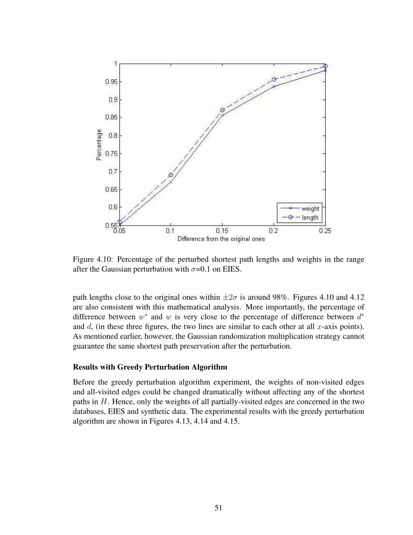
Figure 4.10: Percentage of the perturbed shortest path lengths and weights in the rangeafter the Gaussian perturbation with σ=0.1 on EIES.

path lengths close to the original ones within ±2σ is around 98%. Figures 4.10 and 4.12are also consistent with this mathematical analysis. More importantly, the percentage ofdifference between w∗ and w is very close to the percentage of difference between d∗

and d, (in these three figures, the two lines are similar to each other at all x-axis points).As mentioned earlier, however, the Gaussian randomization multiplication strategy cannotguarantee the same shortest path preservation after the perturbation.

Results with Greedy Perturbation Algorithm

Before the greedy perturbation algorithm experiment, the weights of non-visited edgesand all-visited edges could be changed dramatically without affecting any of the shortestpaths in H . Hence, only the weights of all partially-visited edges are concerned in the twodatabases, EIES and synthetic data. The experimental results with the greedy perturbationalgorithm are shown in Figures 4.13, 4.14 and 4.15.

51

Figure 4.11: Percentage of the perturbed shortest path lengths and weights in the rangeafter the Gaussian perturbation with σ=0.15 on EIES.

52

Figure 4.12: Percentage of the perturbed shortest path lengths and weights in the rangeafter the Gaussian perturbation with σ=0.2 on EIES.

53

(a) EIES

(b) Synthetics

Figure 4.13: Percentage of the perturbed shortest path lengths and weights in the rangeafter the greedy perturbation with 77% targeted pairs being preserved.

54

(a) EIES

(b) Synthetics

Figure 4.14: Percentage of the perturbed shortest path lengths and weights in the rangeafter the greedy perturbation with 54% targeted pairs being preserved.

55

(a) EIES

(b) Synthetics

Figure 4.15: Percentage of the perturbed shortest path lengths and weights in the rangeafter the greedy perturbation with 25% targeted pairs being preserved.

56

The interpretation of these figures is that, for example, in Figure 4.13(a), at x-axis 0.15,the dashed line point (length) is 0.6 (60%) and the solid point (weight) is 0.54 (54%). Itmeans that, after the greedy perturbation algorithm, 54% w∗i,j of the perturbed edges fallintowi,j(1±0.15), and 60% d∗i,j of the perturbed shortest path lengths fall into di,j(1±0.15),in addition to the shortest paths of all targeted pairs in H being exactly preserved.

Figures 4.13, 4.14 and 4.15 are three different experimental results based on variousnumbers of targeted pairs, 77%, 54%, 25%, which are the same shortest paths and theclose lengths of the shortest paths in the two databases. In other words, only 77%, 54%and 25% pairs of all pairs were included in the targeted pair set H , respectively. In ad-dition to the various numbers of targeted pairs, the ratios of partially-visited edges to alledges are 13%, 15% and 9% in EIES, and 19%, 14% and 20% in the synthetic data, re-spectively. For example, in Figure 4.13(a), the number of all edges is 820, but only 13%edges (820*13%=103) are partially-visited edges and under the constraint while the other87% edges could be changed.

From Figures 4.13, 4.14 and 4.15, it is obvious that even a large amount of targetedpairs in H which need keep exactly the same shortest paths and the close lengths of theshortest paths, the perturbed shortest path lengths are still very close to the original ones.In addition to this, the shortest paths of all 77%, 54% and 25% targeted pairs are exactlykept after perturbation, respectively.

4.4 Summary

In consideration of the privacy issue in social network data mining techniques, the link’sweights between social network entities are sensitive in some cases such as the businesstransaction expenses. This chapter addresses a balance between protection of sensitiveweights of network links (edges) and some global structure utilities such as the shortestpaths and the corresponding shortest path lengths.

In this chapter, two perturbation strategies, Gaussian randomization multiplication andgreedy perturbation algorithm, are presented to perturb individual (sensitive) edge weightsand try to keep exactly the same shortest paths as well as their lengths close to those ofthe original social network. The experimental results demonstrate that the two proposedperturbation strategies do meet the expectation of mathematical analysis.

Copyright c© Lian Liu, 2015.

57

Chapter 5 Privacy Preservation of Affinities Social Networks via Probabilistic Graph

The development of digital technology and internet has promoted a proliferation of so-cial networks. Due to the public concern of privacy, the potential of sharing certain socialnetworks may be seriously limited by the need for a balance between the protection ofsensitive content and public accessibility of social networks. So privacy preservation tech-nologies should be employed to protect social networks against various privacy leakagesand attacks. Beyond the ongoing privacy preserving social network studies which mainlyfocus on node de-identification and link protection, issues of preserving the privacy oflink’s affinities, or weights, are studied in a finite and directed social network. To protectthe weight privacy of edges, a privacy measurement, µ-weighted k-anonymity, is definedover individual weighted edges. A µ-weighted k-anonymous edge can make itself more in-distinguishable from adjacent edges with respect to edge weights rather than node degrees.It transforms the original weighted edges to µ-weighted k-anonymous edges, while pre-serving the shortest paths and the corresponding lengths between user-defined node pairsas much as possible. To achieve this goal, a probabilistic graph is proposed to model theweighted and directed social network. Based on this probabilistic graph, random walk,and matrix analysis, a modification algorithm is presented on the weights of edges to ac-complish a balance between the weight privacy preservation and the shortest path utility.Finally, experimental results are given to support the theoretical analysis.

5.1 Background

A social network consists of a set of entities and some intrinsic relationships between theseentities. Although most current social network research focuses on unweighted relation-ships without certain affinities (or weights), it is believed that topologically unweightedrelationships miss the affinity dimension of social networks. On the other hand, adding rel-evant weights into social networks may produce a balanced structure which embeds affinitypatterns into topological metrics. As a result, the affinity enhances understanding about thesocial network, such as the community evolution [156], modular structures [80], politicaltrends [97], terrorist covert subgroups [95], scientific collaborations [129], traffic impor-tance [9], urban sprawl patterns [116]. Therefore, it is of interest to study weighted socialnetworks.

A weighted social network can be simply represented by a graph, where each nodecorresponds to an entity and the weight of each edge between two nodes corresponds toan affinity. Strictly, affinities are the numerical metrics attached to individual edges torepresent meaningful and siginficant relationship. In this chapter, affinities and weights areinterchangeable.

Motivation

Affinities are privacy in a weighted social network. Current research in privacy preserv-ing social networks mainly pays attention to the protection of node attributes, especially

58

node’s identification, via de-identification processes [12, 37, 76, 77, 106, 163, 174, 179,182]. In a weighted social network, the de-identification process without taking weightprivacy into account is not enough to ease public privacy concern for two reasons.

First, node identifications are not considered as privacy in all cases. As said in previousChapter, ArnetMiner [156] allows the creation of the academic research network by miningbibliography databases and researchers’ personal web sites through public web portals. Inthis case, privacy of individual researchers is not a major concern given that these networksare constructed from the public data. So in this case, the node de-identification process isunnecessary.

Second, it is worthwhile noting that some distinguishable weights can be used to re-veal certain sensitive relationships if the weights are not modified in a weighted privacy-preserving social network. For example, in a college cell phone social network, the affinityis represented as the frequencies of cell phone communications between two entities ina period of time. Obviously, a high affinity probably denotes a very close personal re-lationship such as boyfriend or girlfriend. Somebody is probably not willing to disclosethis personal relationship to the public. The exposure of the personally confidential rela-tionship will hinder social data collection. More importantly, distinguishable weights canhelp attackers recover the node identification even if all node are de-identified in terms ofthe unweighted topological structure. For example, a research group consists of a director(the professor) and n-1 graduate research students. In the small social network, everyonehas a connection with each other via the email communication which makes the network acomplete graph on n nodes denoted as Kn. From the unweighted topology point of view,each node is k-anonymous with the remaining nodes [106]. Due to the fact that only thedirector frequently sends group emails such as seminar notes, student meeting announce-ments to all his/her students, the director node is vulnerable to the affinity structure sinceonly the director has a comparatively high frequent email communication to the remainingnodes even if the director node identification is removed and the node is k-anonymous withrespect to the unweighted relationship topology.

Therefore, in addition to the ongoing privacy preserving social networks which mainlyfocus on node de-identification and link protection, the significance about the privacy ofedge weights also deserves to be seriously studied.

How to protect weight privacy. In this chapter, for simplicity, it is assumed thatthe weighted social network is already de-identified but the weights are not modified atthe moment. Some potential affinity privacy-preserving options and the correspondingadvantages and disadvantages are given at first. Then based on this analysis, a problemformulation will be presented in the next subsection.

The first and simple option is that to protect the weight privacy, it is needed to hideor delete weights in social networks. This protection implementation is straightforwardbut problematic. Just hiding weights will not only violate the increasing need for infor-mation sharing about affinities but also seriously limit the utility of the weighted socialnetwork, such as the modular structure [80] which is stored in the weights rather than thegraph node topology. Imagine a scenario that student X would like to apply for a post-doc position under Professor Z. He knows that, in his department, Professors A, B, ..., Thave some relationships with Professor Z (this can be done via arnetminer.org [156] whichcan give an unweighted connection between two scholars). Some professors have a close

59

connection to Professor Z such as co-authors, classmates, even good friends, but some oth-ers are just loosely related to professor Z such as citing Professor Z’s paper. Surely, theclosely connected professors in this department are better to write a recommendation letterto Professor Z than those loosely related professors. The scholar connection’s closeness isendowed with weights. Assume it is not possible to ask all professors to write a letter forstudent X. In such a case, if just these weights are hidden, student X will not know whichprofessor in this department is the best choice to write a useful recommendation letter.

As another option, each edge weight can be either added or multiplied by a non-zeroconstant. This strategy is easily implemented which is inappropriate to keep the weightprivacy and maintain the utility of weighted social networks. In the case that every orig-inal weight is changed to the modified weight by a non-zero constant multiplication, alloriginal weights will be vulnerable if the constant is breached. So constant multiplicationor supplement is not safe to maintain the weight privacy. Alternatively, a non-constantmultiplication or supplement is desirable to avoid potential subgraph privacy collapse. Onthe other hand, some global utilities of the social network depend on the weights such asthe shortest paths [98] which can be applied to measure the probability of the creation of anew edge between nodes. The non-zero constant weight multiplication inflates the lengthsof the shortest paths and further produces a wrong probability of the new edge birth. Sothe preservation of some social network utilities should be taken into consideration in theproblem formulation.

Problem Formulation

Based on the previous analysis, an edge weight modification strategy is proposed to max-imize both information sharing and data utility while at the same time preserve weightprivacy. In this chapter, the data utility of a weighted social network is defined as theshortest paths and their lengths in this network. Compared to a shortest path being a pathwith minimum steps in the unweighted social network, here the shortest path is defined asthe one path whose total sum of the weights of the passing edges is the smallest one amongall possible paths between the node pair in question. The data privacy about weights is re-lated to the discrepancy between the weights of adjacent edges. The discrepancy related toweighted edges should make these edges more indistinguishable from their adjacent edgeswith respect to edge weights.

So, the purpose of this chapter is to modify as many edge weights as possible to achievea given weight privacy standard (i.e., µ-weighted k-anonymity, defined in the later), atthe same time keep the shortest paths the same as the original paths and maintain theircorresponding lengths close to the original lengths.

Contributions

To accomplish the purpose, a weighted graph is reduced to a probabilistic graph. A proba-bilistic graph is a general graph model where the transition probability from one node to theothers defines the affinities between two identities. Although replacing the original weightsby probabilities is a privacy preserving approach to some extent, the privacy concerned inthis chapter goes well beyond this process.

60

A privacy preserving social network is designed in which only the edge weights aremodified to minimize the weight discrepancy without adding or deleting any node andedge, while the shortest paths and the corresponding lengths between user-defined nodepairs in the modified social network are maintained to be as close to the original ones aspossible.

Contributions in this chapter are summarized as follows:

1. A probabilistic graph is constructed in order to inexpensively perform a quantitativeanalysis on data utility and data privacy.

2. The definition of µ-weighted k-anonymous privacy is given to measure the privacylevel of individual edge weights. µ-weighted k-anonymous privacy is proposed overthe continuous weights since the standard k-anonymity, defined on discrete and cat-egorical values [154], is not applicable to continuous values.

3. Based on the proposed single edge weight modification algorithm and the quantita-tive analysis of the modification procedure, an edge frequency order is constructedto achieve the balance between data utility and data privacy.

4. A comprehensive experimental results are illustrated to support the claim about agood balance between privacy and utility.

5.2 Data Utility and Privacy

In this section, a detailed weight modification in accordance with the data utilization andthe privacy preservation will be given. Some preliminaries and notations are first given thatwill be used later.

A social network is defined in this chapter as a weighted and directed graphG={V,E,W}.The nodes of the graph, V , are abstract representation of any meaningful entities. Here,nodes of social networks are not de-identified, especially in identification-public social net-works such as academic collaboration networks. E is the set of all directed and weightededges. One positive numerical weight, wi,j , between node i and node j, is tied to the di-rected edge which reflects the affinity between the two entities. And it is assumed thatall weights in this chapter are positive. If there is no edge between two nodes, the cor-responding weight is denoted as a large enough number and excluded in the modificationalgorithm. The adjacency matrix,W , of the social network is composed of all edge weightswi,j . The shortest path between two different nodes is a path whose total sum of the weightsof the passing edges is the smallest one among all possible paths. The cardinalities of Vand E, n=‖V ‖ and m=‖E‖, are the numbers of nodes and edges in this social network,respectively. Although the algorithm is based on directed graphs, it can be easily extendedto undirected graphs. Each undirected and weighted edge can be transformed into two di-rected edges between the same node pair with opposite directions and the same weightswhile the graph topology is unchanged. It is assumed that Ri,j is the set of all possiblepaths connecting node i and node j, and ri,j is a particular path from node i to node j. Rand r are short for Ri,j and ri,j without otherwise explicitly stated.

61

Data Utility

Before the formal definition about the probabilistic graph, the adjacent edge set Φ(i) of agiven edge (i → j) is defined as Φ(i)={the edge (b → c)| b = i & wb,c 6= 0}. Theadjacent edge set Φ(i) is the set of all edges coming from the same source node i in thegraph. Let γi be the cardinality of Φ(i).

The weight in weighted graphs is transformed into a transition probability as in Defini-tion 5.2.1, based on the adjacency matrix W of a social network.

Definition 5.2.1. The transition probability, pi,j , of a given directed and weighted edge (vi→ vj) is defined as

pi,j =

1wi,j∑γit=1

1wi,t

. (5.1)

Intuitively, an edge with a small weight is more likely to be chosen as a part of theshortest path correspondingly. Since pi,j is inversely related to the weight, based on Defi-nition 5.2.1, an edge with a large pi,j is more likely to be chosen as an edge in the shortestpath than the one with a small pi,j .

The shortest path from node i to node j in weighted graphs is equivalent to a path rwhose probability P (r), defined in Formula (5.2) [173], is highest among all possible pathsbetween the two nodes,

P (r) =exp[−θE(r) + ln P (r)]

Zi,j, (5.2)

where P (r) =∏τ(r)

t=1 pvt,vt+1 , E(r) =∑τ(r)

t=1 wvt,vt+1 , Zi,j =∑

r∈R exp[−θE(r) + ln P (r)],τ(r) is the number of edges in the path r, and θ is a parameter, saying 20 [173]. TheE(r) is the sum of edge weights in the path of weighted graphs, and P (r) is the product ofedge transition probabilities in a path. Formula (5.2) implies that the shortest path has thehighest probability P (r) among all possible paths. Moreover, the smaller E(r) a path has,the higher P (r) it has.

The length of the shortest path between node i and node j in weighted graphs is trans-lated into the expected energy, E, defined as follows [173]:

E =∑r∈Ri,j

exp[−θE(r) + ln P (r)]E(r)

Zi,j. (5.3)

Here, E(r) is the sum of edge weights for any path r (r is not required to be the shortestpath), and E is the length of the shortest path.

From the viewpoint of probabilistic graphs, the shortest path is a path with the highestprobability P (r) and the corresponding length being E. To calculate the possibility of agiven path, the numerator of Formula (5.2), exp[−θE(r) + ln P (r)], is easy to calculategiven the path is known. But the computation of the denominatorZi,j =

∑r∈R exp[−θE(r)+

ln P (r)] is difficult since it requires to enumerate all possible paths. The difficulty in com-puting E is similar. Alternatively, the computation of Zi,j can be transformed into the

62

computation of matrix power series. Before discussing the computation of Zi,j , a matrix Qis defined as:

Q = exp[−θW + ln P ], (5.4)

where, W is the same as W with the exception of the j-th row of W being infinite (inpractice a very large positive number is chosen). P is a matrix composed of pi,j , butthe j-th row of P is 0. For example, the (i, j)-th entry of Q3 (or Q ∗ Q ∗ Q) equalsZi,j =

∑r∈R(3) exp[−θE(r)+ln P (r)], where R(t) denotes a set of paths connecting node

i and node j by t edges.Based on the matrix Q, Z can be computed as:

Z =∑r∈Ri,j

exp[−θE(r) + ln P (r)]

=∞∑t=1

∑r∈Ri,j(t)

exp[−θE(r) + ln P (r)]

=∞∑t=1

Qt. (5.5)

Under the condition i 6= j and the absolute value of maximal eigenvalue of Q is smallerthan 1, Zi,j =

∑∞t=1[Qt]i,j = [(I −Q)−1 − I]i,j = eTi (I −Q)−1ej , where [·]i,j denotes the

(i, j)-th entry of the matrix and ei is the i-th column of an identity matrix with proper di-mension. Here, the computation for the sum of possibilities for all paths can be transformedinto computing the inverse of a matrix.

Similarly, the length of the shortest path, E, is calculated asE = − zTi ∗S∗zjZi,j

(please referto [173] for detail), where, zi, zj and Zi,j are the i-th, j-th columns, and the (i, j)-th entryof the matrix Z, and S = exp[−θW ∗ ln W + ln P ∗ ln W ].

Until now, from the viewpoint of probabilistic graphs, the shortest paths and the corre-sponding lengths between node pairs are introduced. A modification scheme will be pro-posed to approach a balance between privacy preservation of edge weights and utilizationof the shortest path in the next subsection.

Data Privacy

One of the two purposes in this chapter is to protect the weight privacy of the edges. Anedge with an indistinguishable weight is relatively difficult to breach based on the back-ground information about adjacent edges in this social network.

For example, Company A has four directed edges to Agent 1, Agent 2, Agent 3, andAgent 4 with corresponding weights 40, 10, 48, and 43 as in Figure 5.1(a). It is possibleto guess what the edge (Company A→Agent 2) is if background information is availablesuch as that one weight is far more different than the others. But if the weights of the fouredges are very close to each other, like 35, 32, 36, and 33 as in Figure 5.1(b), it is not easyto know which one is the distinguishable edge. Also note that in the modified network as inFigure 5.1(b), the shortest path between Company A and Company D (Company A→Agent

63

Com

pany A

Com

pany D

Agent 2

Agent 4

Agent 5Agent 1

Agent 3

60

5085

48 66

70

43

10

40

90

unit=million/month(a) The Original Network

Com

pany A

Com

pany D

Agent 2

Agent 4

Agent 5Agent 1

Agent 3

70

6570

36 70

70

33

32

35

67

unit=million/month(b) The Modified Network

Figure 5.1: The original business social network and the modified one. In the modifiednetwork, the blue edge group and the green edge group satisfy the 4-anonymous privacywhere µ=10.

64

2→Company D) is the same as the original one in Figure 5.1(a), and the correspondinglength (99) in the modified network is very close to the original one (100) in Figure 5.1(a).

To eliminate the distinguishability between edge weights, µ-weighted k-anonymousweight privacy is defined as follows:

Definition 5.2.2. The edge (i→ j) is µ-weighted k-anonymous if and only if there exist atleast k edges in Φ(i) whose weights wi,tl , l=1, ..., c, and c ≥ k, satisfy ‖wi,j − wi,tl‖ ≤ µ,l=1, ..., c.

Here, µ is a predefined positive parameter to control the degree of privacy and Φ(i) isthe adjacent edge set in which all edges come from the i-th node. Please note that in thecase of the total number of edges in Φ(i) being smaller than k, saying k′ (k′ ≤ k), theedge is µ-weighted k-anonymous if all edges in Φ(i) are not far away more than µ and theweights of at least k-k′ other edges outside Φ(i) are not far away more than µ.

In Figure 5.1(a), the shortest path between Company A and Company D is the path(Company A→Agent 2→Company D), and the corresponding length is 100. But the pri-vacy of the edges in the original network is not good since the adjacent edges are notindistinguishable, i.e., the edge (Company A→Agent 2) is obviously different from thethree others, the edge (Agent 1→Company D) has a big difference from the edge (Agent1→Agent 5), and so do the four incoming edges to Company D. After the weight modifi-cation, as in Figure 5.1(b), most edges are indistinguishable from their adjacent edges asboth the blue edge group and the green edge group satisfy a 4-anonymous privacy, whereµ=10. At the same time, the shortest path in the modified network is the same as the one inthe original network, while the corresponding modified length is 99 and the original one is100.

From the perspective of a probabilistic graph, Definition 5.2.2 is equivalent to the fol-lowing definition.

Definition 5.2.3. The edge (i → j) is µ-weighted k-anonymous if and only if there existat least k edges in Φ(i) whose transition probability pi,tl , l=1, ..., c, and c ≥ k, satisfy‖1/pi,j − 1/pi,tl‖ ≤ µ∆, l=1, ..., c, and ∆=

∑γil=1 1/wi,tl .

Formally, the following theorem is used to decide whether an edge is µ-weighted k-anonymous or not.

Theorem 5.2.1. An edge (i→ j) is µ-weighted k-anonymous if

γi∑l=1

sign(‖ 1

pi,j− 1

pi,tl‖ − µ∆) ≤ γi − k.

Here, sign(·) is a modified sign function such that

sign(x) =

{1 x ≥ 0,0 otherwise.

Theorem 5.2.1 can be proved straightforwardly by using Definition 5.2.3, since theinequality of Theorem 5.2.1 just shows that among all γi neighbors, there are at least k

65

neighbors holding the property ‖ 1pi,j− 1

pi,tl‖ ≤ µ∆. The meaning of Theorem 5.2.1 is that

an edge (i → j) is not µ-weighted k-anonymous (see Definition 5.2.2) if the number ofedges whose weights are more than µ far away from that of this given edge is larger thanγi − k.

Measured over the weighted edges, the µ-weighted k-anonymous privacy definition issubstantially different from the anonymity privacy definition on nodes [76, 77, 94, 103,106, 182]. As mentioned in the introduction, the privacy against the disclosure of nodeinformation is unnecessary in some cases. Furthermore, previous node privacy definitionssuch as k-anonymous nodes [76, 77] and neighborhood attacks [12, 182] are not easy tobe extended to the confidential weights of the edges since edge weights can be continu-ous values and the node privacy definitions are almost essentially based on discrete nodedegrees.

Although it is hoped to construct a social network with any amount of edges to achievethe same data utility and µ-weighted k-anonymous privacy, it is not always possible to doso due to the shortest-path data utilization being a strong constraint when the number ofthe shortest paths to be maintained is large. So, the privacy preserving purpose is to makeas many edges µ-weighted k-anonymous as possible, under the condition of data utility.

5.3 Modification Algorithm

Although there is at least one shortest path between any pairs of nodes in a connected graph,it is reasonable to assume that not all shortest paths are equally important. In addition, ithas been proved in the previous Chapter that it is impossible to modify each weight andpreserve all the shortest paths and the corresponding lengths [108]. It is assumed that thedata owners decide about the subset of all shortest paths to be preserved, denoted as H ,according to their utility demands. For example, at the beginning of weight modification,Bank A requires the privacy-preserving social network server to keep the shortest pathsbetween itself and Bank Z the same as the original one since Bank Z is its most importantbusiness partner. At the moment, Bank A does not know which algorithm the server willimplement and even it does not know the global structure of the whole network. The onlything that data owners have to do is to propose a data utility requirement (i.e., the set H).The task is, given the data utility requirement H , to maximize both the weight privacypreservation and the shortest path utilization H .

The algorithm is given for the single edge modification in Section 5.3, and the methodwill be presented to choose an optimal order to modify multiple edges in Section 5.3.

Single Edge Weight Modification

The change of a single edge weight can affect both the shortest paths passing through it andnot passing through it. To modify the weight wi,j of a given directed and weighted edge(i → j) without changing the set of the shortest paths in H , several conditions needed tobe satisfied and they are listed in Figure 5.2.

Condition 1 implies that the topology of the social network (node structure V =V ∗ andedge structure E=E∗) will not be changed. Conditions 2 and 3 make sure that after the

66

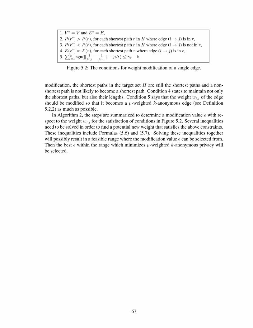
1. V ∗ = V and E∗ = E,2. P (r∗) > P (r), for each shortest path r in H where edge (i→ j) is in r,3. P (r∗) < P (r), for each shortest path r in H where edge (i→ j) is not in r,4. E(r∗) ≈ E(r), for each shortest path r where edge (i→ j) is in r,5.∑γi

l=1 sgn(‖ 1pi,j− 1

pi,tl‖ − µ∆) ≤ γi − k.

Figure 5.2: The conditions for weight modification of a single edge.

modification, the shortest paths in the target set H are still the shortest paths and a non-shortest path is not likely to become a shortest path. Condition 4 states to maintain not onlythe shortest paths, but also their lengths. Condition 5 says that the weight wi,j of the edgeshould be modified so that it becomes a µ-weighted k-anonymous edge (see Definition5.2.2) as much as possible.

In Algorithm 2, the steps are summarized to determine a modification value e with re-spect to the weight wi,j for the satisfaction of conditions in Figure 5.2. Several inequalitiesneed to be solved in order to find a potential new weight that satisfies the above constraints.These inequalities include Formulas (5.6) and (5.7). Solving these inequalities togetherwill possibly result in a feasible range where the modification value e can be selected from.Then the best e within the range which minimizes µ-weighted k-anonymous privacy willbe selected.

67

Algorithm 2 Single edge weight modification algorithm.Input: The weight wi,j of the edge (i → j) and the social network G=(V,E,W ), and the

set H of the selected shortest paths to be maintained.Output: The modification value e with respect to wi,j .

1: Initialize U1=(-∞,+∞)2: for each path r in H do3: if edge (i→ j) is in r then4: solve the inequality, and let its answer be U ′

P (r∗) =exp[−θEnew(r∗) + ln P new(r∗)]

Znewi,j

> P (r) (5.6)

5: else6: solve the inequality, and let its answer be U ′

P (r∗) =exp[−θEnew(r∗) + ln P new(r∗)]

Znewi,j

< P (r) (5.7)

7: end if8: U1=U1 ∩ U ′.9: end for

10: if U1 6= ∅ then11: U2={e | e ∈ U1 & E

new ≈ E}12: else13: EXIT14: end if15: e=argmin

e∈U2

∑γil=1 sgn(‖ 1

pi,j− 1

pi,tl‖ − µ∆)

68

The following shows how to calculate the Formulas (5.6) and (5.7) when the weight ismodified from wi,j to w∗i,j=wi,j+e.

When a weight is updated, its corresponding new transition probability pnewi,j can becomputed based on Definition 5.2.1 as follows:

pnewi,j =

1wi,j+e∑γi

t=1&t6=j1wi,t

+ 1wi,j+e

. (5.8)

Formula (5.8) implies the following information. Firstly, since all weights are positive,the value of e should be larger than −wi,j . Secondly, the change of one edge weight isonly effective in pi,j and has nothing to do with other probabilities. Thirdly, Formula (5.8)is a monotonically decreasing function with respect to e in the range (−wi,j , +∞) byrewriting it into the form of pnewi,j = 1

δ∗(wi,j+e)+1, where δ =

∑γit=1&t6=j

1wi,t

is a constant inthe case of only wi,j being changed. This monotonically decreasing property means thatthe probability pnewi,j will be increasing as long as wi,j is decreasing and vice versa.

The new probability of the shortest path as referred to in Formulas (5.6) and (5.7)concerns both Enew(r∗), P new(r∗) and Znew

i,j . Here the focus is on the computation ofZnewi,j since the rest are straightforward to compute

Enew(r∗) = E(r) + e, (5.9)

and

P new(r∗) = P (r) ∗ pnewi,j

pi,j. (5.10)

How to calculate the numerator and denominator of P (r∗) as in Formulas (5.6) and(5.7) will be discussed in the following paragraphs from the viewpoint of matrix perturba-tion.

Regarding the numerator, exp[−θEnew(r∗)+ln P new(r∗)] = exp[−θ(E(r)+e)+ln(P ∗pnewi,j

pi,j)].

With respect to the denominator, the updating algorithm for Q is proposed first sinceZi,j is related to Q according to Formula (5.5). The new Q, denoted as Qnew, is recon-structed as:

Qnew = exp[−θW + ln P new]

= exp[−θ(W + e) + ln(P ∗ pnewi,j

pi,j)]

= exp(−θe)pnewi,j

pi,jQ, (5.11)

Here, θ is a user-defined parameter and e is the value for the weight modification, pnewi,j isthe updating transition probability of the modified weight w∗i,j as in Formula (5.8), pi,j isthe transition probability of the weight wi,j in the original social network as in Formula(5.1), and Q is the original value as in Formula (5.4). Because Q/pi,j in Formula (5.11) isonly related to the original social network, it is a constant.

69

Znewi,j is the (i, j)-th entry of the matrix (I −Qnew)−1. So, based on Formula (5.11),

Znewi,j = (I −Qnew)−1 = (1−Q+ [β])−1

i,j (5.12)

= (I −Q)−1 − β

1 + βZj,iziz

Tj (5.13)

= Zi,j −β

1 + βZj,iZi,j. (5.14)

Here, β is a scalar whose value is [1− exp(−θe)pnewi,j

pi,j]Q. Zi,j , Zj,i, zi and zj are the (i, j)-th

entry, the (j, i)-th entry, the i-th column and the j-th row of the matrix Z. Because the fouritems have nothing to do with the modification and are known to the data owner, they canbe computed in the preprocessing step to reduce the computational cost. The derivationfrom Formula (5.12) to Formula (5.13) is based Sherman-Morrison-Woodbury formula,(A + UCV )−1 = A−1 − A−1U(C−1 + V A−1U)−1V A−1. Particularly, based on resultsin [30], when the perturbation matrix UCV is a one-entry matrix D, the inversion of theperturbed matrix is as (A+D)−1 = A−1−A−1(1+DB)−1DB, whereA is an n*n positivematrix, D is a one-entry matrix with the (i, j)-th entry being a non-zero number e, A−1 isthe i-th column of A−1, D is e, B is the (j, i)-th entry of A−1, and B is the j-th row of A−1.

A new length of the corresponding shortest path is decided by W ∗ and Znew’s compo-nents (the i-th, the j-th columns and the (i, j)-th entry of Znew). So, the new length of thisshortest path is extended from Equation (5.3) as follows:

Enew

=zTi (W + [e]) ◦ (P ◦ [

pnewi,j

pi,j]) ◦ exp[−θ(W + [e])]zTj

znewi,j

. (5.15)

Here, the operator ◦ is the elementwise matrix multiplication, and zi, zj and znewi,j are the

i-th, the j-th columns and the (i, j)-th entry of Znew. [pnewi,j

pi,j] and [e] are one-entry matrices

with the corresponding values, respectively. The computation of zi, zj and znewi,j is identicalto Formula (5.14).

Therefore, to satisfy Condition 4 in Figure 5.2, Enew

should be close to E which isa fixed value and known to the data owner. Note that if e throughout the computation ofFormula (5.15) is not in the range of Formulas (5.6) and (5.7), this value is discarded andthe bound value is chosen in the range of Formula (5.6) and Formula (5.7), respectively. Ifan optimal weight modification is impossible to choose due to the boundary limitation inFormulas (5.6) and (5.7) at one step, a close length of the shortest path can be obtained inthe modification process of other weights.

Multi-Edge Modification Order

Although all edges can be randomly selected for modification, different orders of modifica-tion do not give the same level of privacy. A special order is discussed to modify the set ofedges in order to achieve a high level µ-weighted k-anonymous privacy while maintainingthe same data utilities. Note that each edge weight is modified only once.

Decreasing an edge weight will increase the probabilities of the paths containing thisedge to be a part of the shortest paths while increasing an edge weight will decrease theirprobabilities. These were shown in Lemma 5.3.1.

70

Lemma 5.3.1.P (r∗) =

exp[−θEnew(r∗) + ln P new(r∗)]

Znewi,j

increases for a negative e and decreases for a positive e. Here Enew(r∗), P new(r∗) andZnewi,j are the functions of e.

Proof.

P (r∗) =exp[−θEnew(r∗) + ln P new(r∗)]

Znewi,j

replace Enew(r∗) and P new(r∗) by Formulas (5.9) and (5.10)

=exp[−θ(E(r) + e) + lnP (r) ∗ p

newi,j

pi,j]

Znewi,j

replace P newi,j by Formula (5.8)

=exp[−θ(E(r) + e) + lnP (r) ∗

1wi,j+e∑γi

t=1&t 6=j1

wi,t+ 1wi,j+e

pi,j]

Znewi,j

.

In the above formula, if assume all other variables are constant and just e is a variable, itcan be concluded that P (r∗) increases for a negative e and decreases for a positive e.

Decreasing the weight of a given edge has two consequences: (1) The probability of theshortest paths going through this edge will increase, i.e., they are still the shortest paths;(2) The probability of the non-shortest paths going through this edge will also increase. Itis possible that they become the shortest paths since their new probabilities have increased.Therefore, there exists a range of the modification value e such that, after the modification,the shortest paths will stay the same, and the non-shortest paths will not become the shortestpaths.

Although the modification range for a high frequency edge is tight, µ-weighted k-anonymous privacy may be achieved by the weight modification of low frequency edgeswhich have a bigger range and are modified later. Based on this observation, all edges aresorted in terms of their presence frequencies in the shortest paths. The weight of one edgewhose presence frequency in the shortest paths is highest is first modified. Such sortingcan achieve a high level µ-weighted k-anonymous privacy.

5.4 Experimental Results

One real database, EIES (Electronic Information Exchange System) Acquaintanceship attime 2, and two synthetic databases will be used for experiments.

The social network in the EIES dataset is a directed and weighted graph in which thedata were collected to measure the acquaintanceship between 48 researchers to show theircooperation in research activities. In addition to the EIES database, to test the efficiency

71

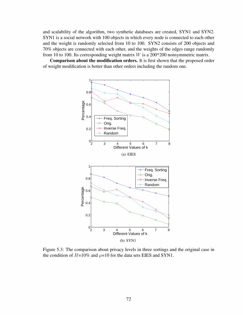
and scalability of the algorithm, two synthetic databases are created, SYN1 and SYN2.SYN1 is a social network with 100 objects in which every node is connected to each otherand the weight is randomly selected from 10 to 100. SYN2 consists of 200 objects and70% objects are connected with each other, and the weights of the edges range randomlyfrom 10 to 100. Its corresponding weight matrix W is a 200*200 nonsymmetric matrix.

Comparison about the modification orders. It is first shown that the proposed orderof weight modification is better than other orders including the random one.

2 3 4 5 6 7 80

0.2

0.4

0.6

0.8

1

Different Values of k

Per

cent

age

Freq. SortingOrig.Inverse Freq.Random

(a) EIES

2 3 4 5 6 7 80

0.2

0.4

0.6

0.8

1

Different Values of k

Per

cent

age

Freq. SortingOrig.Inverse Freq.Random

(b) SYN1

Figure 5.3: The comparison about privacy levels in three sortings and the original case inthe condition of H=10% and µ=10 for the data sets EIES and SYN1.

72

2 3 4 5 6 7 80

0.2

0.4

0.6

0.8

1

Different Values of k

Per

cent

age

Freq. SortingOrig.Inverse Freq.Random

Figure 5.4: The comparison about privacy levels in three sortings and the original case inthe condition of H=10% and µ=10 for the data set SYN2.

In Figures 5.3(a), 5.3(b), and 5.4, the y-axis is the percentage of µ-weighted k-anonymousedges (see Definition 5.2.2), and the x-axis is the different values of k. In Figures 5.3(a),5.3(b) and 5.4, the Freq. Sorting is the descending frequency sorting, the Orig. is theprivacy level of the original social network, the Inverse Freq. is the ascendent frequencysorting, and the Random is one random sorting. For Figure 5.3(a), the Frequent SortingLine at k=3 is 0.94. It means that after perturbation in a frequent ascending order, thereexists 94% edges each of which has at least k-1 (=2) other edges whose lengths meet|ei-ej| ≤ µ. These figures show that the frequency sorting can achieve a higher level of µ-weighted k-anonymous privacy compared to other two sortings in all three social networkswith different values of k.

Comparison about different sizes of H . The efficiency of the edge weight modifica-tion is really dependent on the ratio of the size of H to all node pairs in a social network.The more shortest paths and the corresponding lengths to preserve, the less room of privacyimprovement it can achieve. So several different sizes of H are chosen such as 5%, 10%,15%, 20%, and 25% of all nodes pairs in order to test this algorithm. All the node pairs inH are randomly selected. The parameter θ is chosen as 20.

The purpose of these experiments is to show three things. 1). The ratio of µ-weightedk-anonymous edges to all edges. 2). The percentage of the shortest paths with respect tothe node pairs ofH in the modified social network is the same as the real one in the originalsocial network. 3). The ratio of the length difference between the modified shortest pathand the original one to the length of the original shortest path. The first criterion denotesthe degree of weight privacy preservation, and the second and third criteria stand for theshortest path utilization.

73

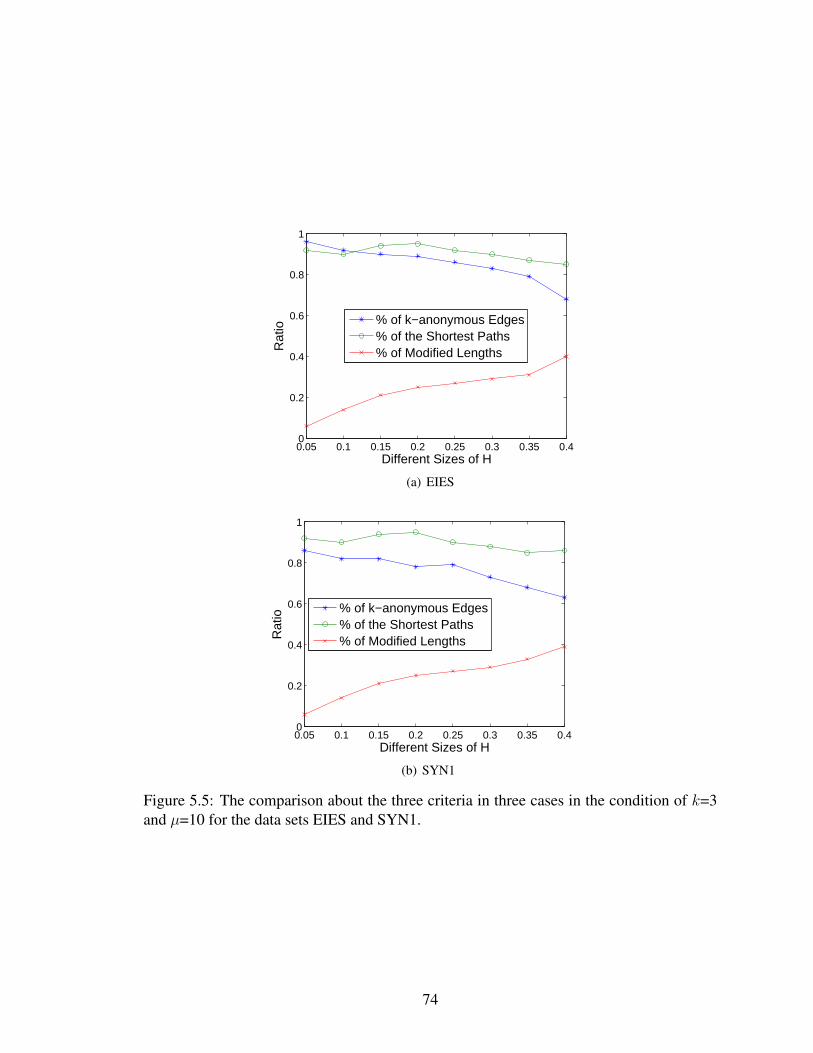
0.05 0.1 0.15 0.2 0.25 0.3 0.35 0.40

0.2

0.4

0.6

0.8

1

Different Sizes of H

Rat

io

% of k−anonymous Edges% of the Shortest Paths% of Modified Lengths

(a) EIES

0.05 0.1 0.15 0.2 0.25 0.3 0.35 0.40

0.2

0.4

0.6

0.8

1

Different Sizes of H

Rat

io

% of k−anonymous Edges% of the Shortest Paths% of Modified Lengths

(b) SYN1

Figure 5.5: The comparison about the three criteria in three cases in the condition of k=3and µ=10 for the data sets EIES and SYN1.

74

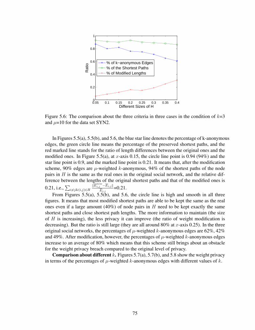
0.05 0.1 0.15 0.2 0.25 0.3 0.35 0.40

0.2

0.4

0.6

0.8

1

Different Sizes of H

Rat

io

% of k−anonymous Edges% of the Shortest Paths% of Modified Lengths

Figure 5.6: The comparison about the three criteria in three cases in the condition of k=3and µ=10 for the data set SYN2.

In Figures 5.5(a), 5.5(b), and 5.6, the blue star line denotes the percentage of k-anonymousedges, the green circle line means the percentage of the preserved shortest paths, and thered marked line stands for the ratio of length differences between the original ones and themodified ones. In Figure 5.5(a), at x-axis 0.15, the circle line point is 0.94 (94%) and thestar line point is 0.9, and the marked line point is 0.21. It means that, after the modificationscheme, 90% edges are µ-weighted k-anonymous, 94% of the shortest paths of the nodepairs in H is the same as the real ones in the original social network, and the relative dif-ference between the lengths of the original shortest paths and that of the modified ones is0.21, i.e.,

∑i 6=j&(i,j)∈H

‖Enewi,j −Ei,j‖Ei,j

=0.21.From Figures 5.5(a), 5.5(b), and 5.6, the circle line is high and smooth in all three

figures. It means that most modified shortest paths are able to be kept the same as the realones even if a large amount (40%) of node pairs in H need to be kept exactly the sameshortest paths and close shortest path lengths. The more information to maintain (the sizeof H is increasing), the less privacy it can improve (the ratio of weight modification isdecreasing). But the ratio is still large (they are all around 80% at x-axis 0.25). In the threeoriginal social networks, the percentages of µ-weighted k-anonymous edges are 62%, 42%and 49%. After modification, however, the percentages of µ-weighted k-anonymous edgesincrease to an average of 80% which means that this scheme still brings about an obstaclefor the weight privacy breach compared to the original level of privacy.

Comparison about different k. Figures 5.7(a), 5.7(b), and 5.8 show the weight privacyin terms of the percentages of µ-weighted k-anonymous edges with different values of k.

75

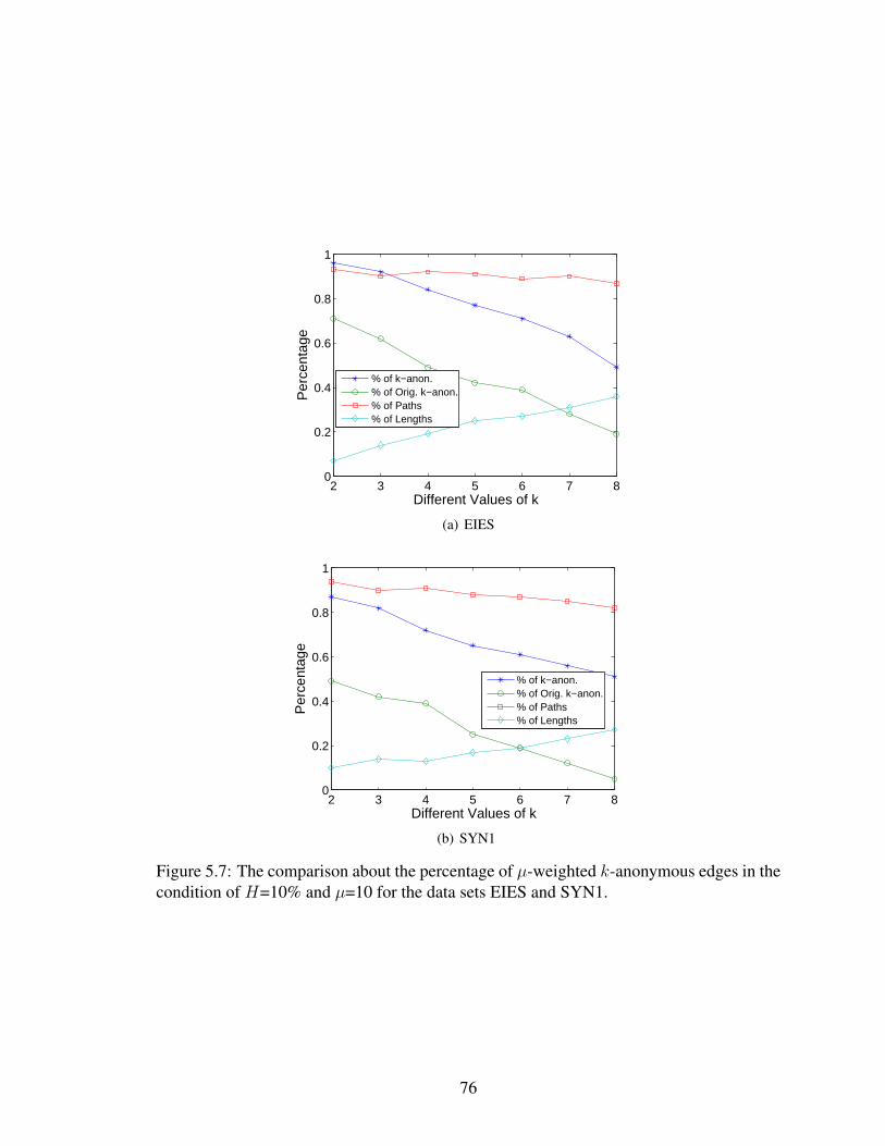
2 3 4 5 6 7 80

0.2

0.4

0.6

0.8

1

Different Values of k

Per

cent

age

% of k−anon.% of Orig. k−anon.% of Paths% of Lengths

(a) EIES

2 3 4 5 6 7 80

0.2

0.4

0.6

0.8

1

Different Values of k

Per

cent

age

% of k−anon.% of Orig. k−anon.% of Paths% of Lengths

(b) SYN1

Figure 5.7: The comparison about the percentage of µ-weighted k-anonymous edges in thecondition of H=10% and µ=10 for the data sets EIES and SYN1.

76

2 3 4 5 6 7 80

0.2

0.4

0.6

0.8

1

Different Values of k

Per

cent

age

% of k−anon.% of Orig. k−anon.% of Paths% of Lengths

Figure 5.8: The comparison about the percentage of µ-weighted k-anonymous edges in thecondition of H=10% and µ=10 for the data set SYN2.

In Figures 5.7(a), 5.7(b), and 5.8, the blue star line denotes the percentage of k-anonymousedges in modified networks, the green circle line means the percentage of k-anonymousedges in original networks, the red squared line stands for the preserved shortest paths, andthe cyan diamond line is the ratio of length differences between the original ones and themodified ones. In Figures 5.7(a), 5.7(b), and 5.8, the green circle line denotes the ratioof the number of µ-weighted k-anonymous edges to that of all edges in the original socialnetworks, and the blue star line means the µ-weighted k-anonymous edge ratio in the mod-ified one. It can be seen that both the privacy level (circle line) in the original network andthe privacy (star line) in the modified social network are decreasing as the value of k is in-creasing. But there are remarkable privacy differences between all original social networksand the corresponding modified networks. It demonstrates that the scheme can definitelyincrease the privacy preservation of original social networks to a noticeably higher level indifferent privacy protection requirements such as various k. More importantly, the preser-vation probability of the shortest paths (square line) are still maintained at a smooth levelsince the shortest-path utility is kept before the data privacy. Although the lengths of theshortest paths (cyan diamond line) in modified social networks increase as k increases, theslope is not so sharp as the corresponding lines (red mark line) in Figures 5.5(a), 5.5(b),and 5.6. It implies that the relative difference between the lengths of the original shortestpaths and that of the modified ones is more affected by the size of H rather than k.

5.5 Summary

In consideration of the privacy issue in social network data mining applications, the link’sweights between social network entities are sensitive in some cases such as in the businesstransaction expenses. This chapter addresses a balance between the protection of sensitiveweights of network links (edges) and two global structure utilities, the shortest paths andthe corresponding shortest path lengths.

77

In this chapter, one algorithm is presented based on random walk and matrix analysis tomodify individual (sensitive) edge weights and try to keep exactly the same shortest pathsas well as their lengths close to those of the original social network. These experimentalresults demonstrate that the proposed modification strategy does meet the expectation ofmathematical analysis.

Copyright c© Lian Liu, 2015.

78

Chapter 6 Differential Privacy in the Age of Big Data

In the previous chapters, privacy protection is applied on numerical data in the form oftables, represented by matrices in Chapters 2 and 3, and Social Networks (SNs for short),described as weighted graphs in Chapters 4 and 5. These proposed privacy preserving al-gorithms are immune from specific privacy attacks on confidential numerical data sets withthe help of a variety of perturbation methodologies, such as SVD, wavelet transformation,Gaussian noises addition, and so on. These techniques, however, have two drawbacks asfollows.

First, all previous algorithms presented in the first part of this dissertation perturb anoriginal confidential data d to a public version d=d+e, and release d instead of d to thepublic, where e is either an additive or reduced noise. From the perspective of public users,only d is accessible and hence the confidential information of the original data d is hidden,while d may maintain desired properties which can benefit future statistical analyses ordata mining applications. But it is not easy for data owners to link d or e to a reasonableprivacy definition.

Second, due to lack of a general privacy definition, the previous algorithms of Chap-ters 3, 4, and 5 cannot protect sensitive data from general privacy violations with strongassumptions. Here, assumptions include limited accessibility to auxiliary information andcomputationally-bounded ability. For example, the original salaries of four anonymouspersons in a community are d = {78082, 250821, 45614, 15286}, and after perturbation,d = {83712, 236523, 51356, 21563}. In this case, although the real sensitive salaries areprotected, hackers can still associate d2 = 236523 with Bob with a high confidence be-cause there is only one surgeon, Bob, in the middle-class community and further concludethat the real salary for Bob should be close to 240000. In fact, Ganta et al. [66] recognizedindividuals from a k-anonymized census data set with the aid of public auxiliary informa-tion. Another famous re-identified example is the breach of the Netflix prize competitionin which Narayanan and Shmatikov [127] de-anonymized a carefully anonymized movieratings data set by the public IMDB Database Statistics. Backstrom et al. [12] also re-identified a majority of anonymous social network accounts by a small subset of knownusers.

Third, data owners have to look for different solutions for various domains because ofinflexibility of previous algorithms in different spaces. For instance, perturbation-basedtechniques are good in a numerical domain, but they cannot be easily extended to otherdomains, like frequent itemset mining whose outputs are sets rather than numbers.

To overcome the above mentioned downsides of traditional perturbation-based algo-rithms, differential privacy was proposed in 2006 [45] with the intention to provide a gen-eral and robust privacy framework for a rich body of domains and tasks. Roughly speaking,as a recent de facto privacy preserving model, differential privacy quantitatively boundsthe contribution of a single original data record to the perturbed output. For instance, ifthe probability of the perturbed output S of an original data set D in any domain R isPr(S ∈ R), the probabilities of corresponding perturbed outputs of the data sets D − {d}and D+ {d} in R are at most exp(k

ε)Pr(S ∈ R), where D is the set of all original individ-

79

ual data, S is the output of D by a differential privacy preserving algorithm, and d is anysingle original data record which can be either d ∈ D or d /∈ D. D − {d} and D + {d}mean set deletion and set union. ε is a predefined privacy parameter, and k is a query-basedconstant which will be explained later.

A detailed coverage about concepts of differential privacy will be shown in Section6.2, including core concepts, promising potentials to unravel the above mentioned threedrawbacks.

A similar privacy preserving technique to differential privacy is SMC (Secure Multi-party Computation) which proposes a method for multiple parties to compute a numericalfunction over individual private data. The differences between the two lie in two aspects.First, SMC is essentially a subfield of cryptography which needs cooperation of multipleparties, but differential privacy is a stand-alone technique which only depends on two pre-defined parameters. Second, differential privacy is a general privacy preservation model,and it can satisfy a variety of tasks at the same time since it is a perturbation-based method.For different tasks, however, SMC has to choose different schemas because it is based on acryptographic computation.

Differential privacy attracts a large amount of researchers’ attention in a line of variousdisciplines. However, little attention is devoted to the combination of differential privacyand big data. The second part of this dissertation from Chapter 6 to Chapter 9 will shedlight on this combination. In Section 6.1, a brief roadmap to individual chapters in thesecond part of this thesis will be introduced, as well as contributions.

6.1 A Roadmap to the Following Chapters and Contributions

Big data is referred to collected information with the quantity being increasing in anexponential fashion. Briefly, this dissertation focuses on three issues in the age of bigdata, obtaining a high confidence about the accuracy of any specific differentially privatequery, speedily and accurately updating a private summary of a binary stream with theI/O-awareness, and launching a mutual private information retrieval for a big data set.

The Chernoff Bound is the backbone to handle the three issues. To put it simply, theChernoff Bound states that for N variables with the same or different distributions in [0,1], only n2 samples (n2 << N ) are enough to approximate some statistical properties, likesum, of all variables. Analogously, the n2 samples serve as the ”eigenvector” or ”basis” forthe entire data set.

Fast approximation to a big data set. By the Chernoff Bound, n2 samples (n2 << N )are enough to approximate the sum of N numbers in a speedy way. Because of the fastapproximation, a high confidence about the accuracy of any specific private query can beobtained.

Capability to speedily and accurately update statistical properties on a time-seriesdata set with the I/O-awareness. To update the holistic statistical properties, like sum,mean, and top-k, only n2 samples instead of the entire time-series with the size N areneeded to fetch. If n2 is independent of N , I/O operations can be significantly reduced to areasonable level for big data.

Mutual private information retrieval for big data. To protect privacy of both users’queries and data centers’ confidential data, the query and the data set to be queried should

80

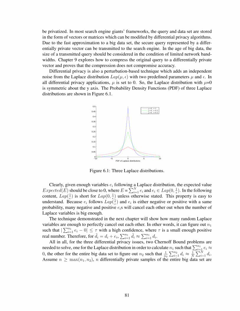
be privatized. In most search engine giants’ frameworks, the query and data set are storedin the form of vectors or matrices which can be modified by differential privacy algorithms.Due to the fast approximation to a big data set, the secure query represented by a differ-entially private vector can be transmitted to the search engine. In the age of big data, thesize of a transmitted query should be considered in the condition of limited network band-widths. Chapter 9 explores how to compress the original query to a differentially privatevector and proves that the compression does not compromise accuracy.

Differential privacy is also a perturbation-based technique which adds an independentnoise from the Laplace distribution Lap(µ, ε) with two predefined parameters µ and ε. Inall differential privacy applications, µ is set to 0. So, the Laplace distribution with µ=0is symmetric about the y axis. The Probability Density Functions (PDF) of three Laplacedistributions are shown in Figure 6.1.

−10 −5 0 5 100

0.05

0.1

0.15

0.2

0.25

0.3

0.35

0.4

0.45

0.5

PDF of Laplace distributions

µ=0, ǫ=1µ=0, ǫ=0.5µ=0, ǫ=0.2

Figure 6.1: Three Laplace distributions.

Clearly, given enough variables ei following a Laplace distribution, the expected valueExpected(E) should be close to 0, whereE =

∑Ni=1 ei and ei ∈ Lap(0, 1

ε). In the following

content, Lap(1ε) is short for Lap(0, 1

ε) unless otherwise stated. This property is easy to

understand. Because ei follows Lap(1ε) and ei is either negative or positive with a same

probability, many negative and positive eis will cancel each other out when the number ofLaplace variables is big enough.

The technique demonstrated in the next chapter will show how many random Laplacevariables are enough to perfectly cancel out each other. In other words, it can figure out n1

such that |∑n1

i=1 ei − 0| ≤ τ with a high confidence, where τ is a small enough positivereal number. Therefore, for di = di + ei,

∑n1

i=1 di ≈∑n1

i=1 di.All in all, for the three differential privacy issues, two Chernoff Bound problems are

needed to solve, one for the Laplace distribution in order to calculate n1 such that∑n1

i=1 ei ≈0, the other for the entire big data set to figure out n2 such that 1

n2

∑n2

i=1 di ≈ 1N

∑Ni=1 di.

Assume n ≥ max(n1, n2), n differentially private samples of the entire big data set are

81

chosen,

1

n

n∑i=1

di

=1

n

n∑i=1

(di + ei)

=1

n

n∑i=1

di +1

n

n∑i=1

ei

≈ 1

n

n∑i=1

di + 0

≈ 1

N

N∑i=1

di.

Based on the above deduction, 1n

∑ni=1 di ≈ 1

N

∑Ni=1 di. Hence, the n differentially private

samples can accurately approximate the original data set∑N

i=1 di, where N >> n.Contributions from Chapter 7 to Chapter 9 are as follows.

1. The accuracy analysis of statistical properties of the standard differential privacymechanism over any subset of data sets is proposed, including sum, mean, min, andmax.

2. Quantitative calculation of n samples is given for N Laplace variables (n << N )such that |∑n

i=1 ei − 0| ≤ τ with a high confidence, where ei follows Lap(1ε).

3. Using n samples to accurately approximate statistical properties of big data in adifferential privacy way is demonstrated in detail.

4. How to compress a confidential vector to a differentially private one is presented.

5. The accuracy compromise of the multiplication of two differentially private vectorsis also analyzed.

The description of aforementioned contributions is a brief summary. In each chapter, adetailed contribution, including the accuracy improvements and reduced time and/or spacecomplexities, will be mentioned, as well as challenges.

An introduction to differential privacy is given in Section 6.2, which serves as the pre-liminary background for following chapters.

6.2 Preliminaries about Differential Privacy

Differential privacy was first proposed by Cynthia Dwork [45] in 2006, and the core con-cepts were developed by McSherry and Talwar who also fostered an exponential mecha-nism [113] in 2007 and PING [112], a differential privacy query platform. Ilya Mironovet al. [120] gave a computationally differential privacy mechanism in 2009. Dwork et al.

82

[51, 50] extended the standard differential privacy to pan privacy for streaming data setsin 2010, and they [51, 50] first distinguished privacy from security. The difference willbe recalled briefly later in this section. After that, a number of researchers were involvedin developing applications or theories. Readers can refer to surveys [46, 47, 149] as acomprehensive understanding.

Core concepts of differential privacy include inputs (original data sets), outputs (re-leased perturbed data sets), queries, randomized mechanisms, neighboring data sets, theglobal sensitivity, and the Laplace distribution, which are introduced one by one in detailand illustrated by examples.

Definition 6.2.1. A data set D is a set of (individual) records in a data universe X .

DN is a data set with the cardinality of N . Accordingly, DN→∞ has an infinite size,e.g., a time-series. For simplicity, the superscript N of DN is dropped if it is clear from thecontext. In the following chapters, D is the data set consisting of original sensitive data.

Definition 6.2.2. A query f is a function such as f : D → R, where D serves as the input,and R is the set of real numbers.

For example, assume D={persons in Kentucky who smoke frequently}, and f is aquery that counts the cardinality of D.

Definition 6.2.3. D and D′

are neighboring data sets, iff 1). D ∈ X and D′ ∈ X ; 2).

max(|D − D′ |, |D′ − D|) ≤ 1. Here, D − D

′is the set deletion, and |D − D

′ | is thecardinality of the set D −D′ .

Please note that D−D′ is not the same as D′ −D. For instance, D={Alice, Bob, Carl,David, Elvis}, andD′={Alice, Carl, David, Elvis}. Then,D−D′={Bob}, andD′−D = ∅.

No matter if Bob ∈ D={persons in Kentucky who smoke frequently} or not, D andD-{Bob} are neighboring data sets, as are D and D+{Bob}, D-{Bob} and D+{Bob}.

For example,D={Alice, Bob, Carl, David, Elvis}, i.e., Bob∈ D. Then,D-{Bob}={Alice,Carl, David, Elvis}, D+{Bob}={Alice, Bob, Carl, David, Elvis}. Hence,

• max(|D − (D − {Bob})|, |(D − {Bob}) −D|)= max(|{Bob}|, |∅|) = 1, so D andD-{Bob} are neighboring data sets.

• max(|D−(D+{Bob})|, |(D+{Bob})−D|)= max(|∅|, |∅|) = 0, soD andD+{Bob}are neighboring data sets.

• max(|(D+{Bob})−(D−{Bob})|, |(D−{Bob})−(D+{Bob})|)= max(|{Bob}|, |∅|) =1, so D+{Bob} and D-{Bob} are neighboring data sets.

The second example isD={Alice, Carl, David, Elvis}, i.e., Bob /∈ D, andD-{Bob}={Alice,Carl, David, Elvis}, D+{Bob}={Alice, Bob, Carl, David, Elvis}. Hence,

• max(|D − (D − {Bob})|, |(D − {Bob}) − D|)= max(|{∅}|, |∅|) = 0, so D andD-{Bob} are neighboring data sets.

83

• max(|D − (D + {Bob})|, |(D + {Bob}) −D|)= max(|∅|, |{Bob}|) = 1, so D andD+{Bob} are neighboring data sets.

• max(|(D+{Bob})−(D−{Bob})|, |(D−{Bob})−(D+{Bob})|)= max(|{Bob}|, |∅|) =1, so D+{Bob} and D-{Bob} are neighboring data sets.

Definition 6.2.4. A randomized mechanismA is a function over any query f : A(f(X ))→R.

Definition 6.2.5. [45] A randomized mechanism A is ε-differentially private or simply ε-private, if for any two neighboring data sets D and D

′and any subset S ∈ R,

Pr[A(f(D)) ∈ S] ≤ exp(ε)Pr[A(f(D′)) ∈ S], (6.1)

where Pr[·] is a probability and exp() is the exponential function with the natural base.Equation (6.1) can be transformed to

Pr[A(f(D)) ∈ S]

Pr[A(f(D′)) ∈ S]≤ exp(ε).

Assume D={persons in Kentucky who smoke frequently} and D′ = D + {Bob} (notethat possibly D=D′ if Bob ∈ D), D and D′ are neighboring data sets, and f is a countingfunction. Suppose S is the set {x≥439,529}, namely 10% of the total estimated populationof Kentucky in 2013 [2]. Definition 6.2.5 can guarantee the probabilistic contribution ofany single original data to the output at most at scale exp(ε). This explanation has twodifferent versions. First, the presence or absence of any single sensitive data cannot changethe output too much. Second, a stronger description of differential privacy is as follows.Assume the first hacker knows nothing about D, and the probability of breaching whetherBob is inD is Pr(x). Suppose the second hacker knows allN -1 persons inD (Bob is not inthe group of theN -1 persons), the probability of breaching whether Bob is inD is boundedat most exp(ε)Pr(x). Here, ”breach” means that a hacker can make sure the absence orpresence of a person inD. In healthcare statistical surveys, for instance, differential privacycan safeguard a patient’s disease even if the number of this particular disease holders is verysmall (even just one). Because even only one person has this disease and hackers know themedical records of all other N -1 persons, differential privacy can obscure the output whichcannot benefit breach of the health condition of the last unknown person.

Regarding the crucial privacy parameter ε, Hsu et al. [81] surveyed the choice of ε. Inmost applications, the predefined privacy parameter ε is small, like from 0.1 to 1. Whenε=0.1, exp(0.1)≈ 1.105. In other words, the probability that hackers can violate dN , thelast unknown person, with the help of {d1, d2, ..., dN−1}, where di is the i-th original dataof D, is only increasing 10.5% at most, compared to no knowledge of {d1, d2, ..., dN−1}.

Clearly, the smaller ε is, the better privacy but the worse accuracy can be attained. Notethat ”accuracy” expresses how the perturbed data is close to the original one. The formaldefinition about accuracy will be presented in the next chapter. Moreover, accuracy andutility are interchangeable. In Figure 6.1, the PDF of a Laplace distribution with a small εdisperses more widely than the one with a big ε. Namely, the majority of Laplace noises

84

with a big ε will fall in a narrow range around the y axis. Hence, a large number of di willbe in close proximity to di, for di=di+ei.

A weaker version, (ε, δ)-differential privacy, is given as follows.

Definition 6.2.6. [45] A randomized mechanism A is (ε, δ)-differential private if, for anytwo neighboring data sets D and D

′and any subset S ∈ R,

Pr[A(f(D)) ∈ S] ≤ exp(ε)Pr[A(f(D′)) ∈ S] + δ,

where Pr[·] is a probability and exp() is the exponential function with the natural base.

Before [51], researchers always think that ”security” and ”privacy” are interchangeable.Actually, they should have different implications in privacy preserving data mining. Pri-vacy is a protection over the public disclosure against possible linkage and reconstructionof confidential information, while security should be thought of a state free from break-insand embezzlements [93]. Specifically, for example, after collecting a confidential data dfrom some sources, a perturbed version d = d + e is released to the public. A perturbationmechanism is designed to increase the burden of rebuilding any private property of d basedon d. The difficulty of reconstruction is called ”privacy”. For security, data owners shouldprotect d after collection processes and prior to any perturbation mechanism, because dstored inside a security system can be probably stolen because of break-ins and embezzle-ments. One way to protect data security is the cryptographic mechanism. In detail, aftercollecting a confidential data, the original data should be encoded before it proceeds to thenext stage, like storage and calculation. Likewise, when collecting a confidential data at in-put portals, pan-differential privacy perturbs it immediately and sends the perturbed one tostorage for future bulk calculation in which all private data proceed to the next perturbationmechanism. Formal definitions about pan-privacy are as follows.

Definition 6.2.7. Assume I is one internal state of a mechanismA. Given any private dataD, ID is output of any partial portion of D processed by any partial procedure. A is ε-panprivate against a single inside intrusion, if for any two neighboring confidential data setsD ∈ X and D

′ ∈ X , any one internal state I , and any subset S in the output domain R,Pr[A(ID) ∈ S] ≤ exp(ε)Pr[A(ID′ ) ∈ S].

Definition 6.2.8. Assume I is set of internal states of a mechanism A, and |I| = t. Givenany private data D, I tD is output of any partial portion of D processed by any partialprocedure at any t different stages. A mechanism is ε-pan private against multiple insideintrusions, if for any two neighboring confidential data sets D ∈ X and D

′ ∈ X , anyset of internal states I , and any subset St in the output domain Rt, Pr[A(I tD) ∈ St] ≤exp(ε)Pr[A(I t

D′) ∈ St].

Consider the example D={persons in Kentucky who smoke frequently} and D′

=D + {Bob}. Data owners would disclose differentially-private numbers of smokers fromdifferent counties of Kentucky. After gathering dfayette from input portals, pan-privacy re-quires data owners to perturb it immediately before it is saved to the memory or the harddrive with the intention to avoid security violation by break-ins.

85

Laplace Mechanisms

This section will introduce how to find a differentially private mechanism A for querieswhose outputs are in R, such as calculation of mean, max, min, sum, and so forth. On theother hand, there are a bunch of queries whose outputs are not in R. For example, algo-rithms for frequent itemset mining should publish items/sets instead of real numbers. TheExponential Mechanism is designed to address this issue [113]. Because this dissertationdoes not touch nominal problems, the introduction to the Exponential Mechanism is omit-ted. Further studies in this direction can be found in [113]. After the introduction to theLaplace Mechanism, three differential privacy’s appealing properties will be demonstratedin Section 6.2, and the promising benefits and limitations of differential privacy will bedescribed in Section 6.2.

Basically, for queries whose outputs are inR, differential privacy is also a perturbation-based algorithm. Its perturbation only hinges on the nature of queries and the privacy levelε, but is independent of the original input data domain X .

Definition 6.2.9. The global sensitivity of a query function f in X is ∆f = max∀D,D′∈X |f(D)−f(D

′)|.

∆f depends on the query function f and the domain X , and it has nothing to do with aparticular input data set. So, the global sensitivity of a query function f is data independent.

Proposition 6.2.1. If X is the population with any certain properties and f is the countingfunction, ∆f=1.

Proof. Let two neighboring data sets beD = {d1, ..., dN , dN+1} andD′ = {d1, ..., dN , d′N+1}.

It is unknown if dN+1 ∈ D′ and d′N+1 ∈ D.f(D) = f({d1, ..., dN}) + f({dN+1}), and f(D

′) = f({d1, ..., dN}) + f({d′N+1}).

max |f(D)− f(D′)| = max |f({d1, ..., dN}) + f({dN+1})− f({d1, ..., dn})− f({d′N+1}|

= max |f({dN+1})− f({d′N+1})|= max |f({dN+1} − {d

′

N+1})|≤ 1.

Note {dN+1} − {d′N+1} = Ø, if dN+1 = d′N+1, otherwise {dN+1}.

One of popular differential privacy mechanisms can be obtained by adding a noise efrom a Laplace distribution.

Theorem 6.2.1. [45] The Standard Laplace Mechanism

A(f(D)) = f(D) + e, (6.2)

where D is any original data set in X , e is independent of f(D), and e follows Lap(∆fε

),is ε-differential private. Here, ∆f is in relation to the query f and X .

86

The proof for Theorem 6.2.1 can be found in [45]. Before the explanation why theLaplace distribution can satisfy ε-differential privacy, a basic knowledge about the Laplacedistribution should be given.

A Laplace distribution can be determined by two parameters, µ and b. Its PDF (Proba-bility Density Function) is as follows:

f(x|µ, b) =1

2bexp(−|x− µ|

b). (6.3)

Based on Equation (6.3), µ is the mean of the Laplace distribution Lap(µ, b). ThreeLaplace distributions can be seen in Figure 6.1. In most applications focusing on differen-tial privacy, µ=0, and b is replaced by ∆f

ε. To follow conventions in this field, Lap(µ, b) is

replaced by Lap(∆fε

) henceforth. In the case of A(f(Di)) = f(Di) + e, Di is the originaldata and e is an independent noise from Lap(∆f

ε). Fixing Di, Pr(A(f({Di})) <= t) =

Pr(f({Di}) + e <= t) =Pr(e <= t− f(Di)) = PDF ( ε2∆f∗ exp(− |t−f(Di)|ε

∆f)).

Next, the reason why the Laplace distribution can satisfy ε-differential privacy will beshown. Given two neighboring data sets D and D′ , a query function f , any subset S ∈ R,and any value t ∈ S,

Pr(t = A(f(D)))

Pr(t = A(f(D′))

=Pr(t = f(D) + e1)

Pr(t = f(D′) + e2)

=Pr(e1 = t− f(D))

Pr(e2 = t− f(D′))

=PDF (t− f(D))

PDF (t− f(D′))

=

ε2∆f

exp(− (t−f(D))ε∆f

)

ε2∆f

exp(− (t−f(D′ ))ε∆f

)

= exp((−t+ f(D) + t− f(D

′))ε

∆f)

= exp((f(D)− f(D

′))ε

∆f)

≤ exp(ε).

Until here, although differential privacy is also a perturbation-based technique, a jus-tified privacy protection model between a random noise and a reasonable privacy require-ment can be rigorously built.

There are two basic places where the perturbation can happen, input perturbation andoutput perturbation.

Back to the example D={persons in Kentucky who smoke frequently}, all personsin Kentucky are in the input domain. If the i-th person in Kentucky is a smoker, di=1,otherwise 0. For input perturbation, di = di + e, and then A(f(D)) =

∑Ni=1 di. di is

87

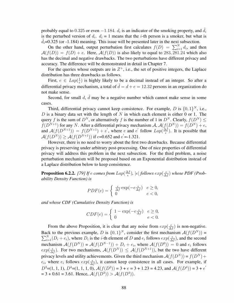
probably equal to 0.325 or even −1.184. di is an indicator of the smoking property, and diis the perturbed version of di. di = 1 means that the i-th person is a smoker, but what isdi=0.325 (or -1.184) meaning. This issue will be presented later in the next subsection.

On the other hand, output perturbation first calculates f(D) =∑N

i=1 di, and thenA(f(D)) = f(D) + e. Here, A(f(D)) is also likely to equal to 283, 281.24 which alsohas the decimal and negative drawbacks. The two perturbations have different privacy andaccuracy. The difference will be demonstrated in detail in Chapter 7.

For the queries whose outputs are in Z+, i.e., the set of positive integers, the Laplacedistribution has three drawbacks as follows.

First, e ∈ Lap(1ε) is highly likely to be a decimal instead of an integer. So after a

differential privacy mechanism, a total of d = d+ e = 12.32 persons in an organization donot make sense.

Second, for small d, d may be a negative number which cannot make sense in somecases.

Third, differential privacy cannot keep consistence. For example, D is {0, 1}N , i.e.,D is a binary data set with the length of N in which each element is either 0 or 1. Thequery f is the sum of DN , or alternatively f is the number of 1 in DN . Clearly, f(DN) ≤f(DN+1) for any N . After a differential privacy mechanism A, A(f(DN)) = f(DN) + e,and A(f(DN+1)) = f(DN+1) + e

′ , where e and e′ follow Lap(∆fε

). It is possible thatA(f(DN)) ≥ A(f(DN+1)) if e=0.652 and e′=-1.321.

However, there is no need to worry about the first two drawbacks. Because differentialprivacy is preserving under arbitrary post-processing. One of nice properties of differentialprivacy will address this problem in the next subsection. For the third problem, a noiseperturbation mechanism will be proposed based on an Exponential distribution instead ofa Laplace distribution below to keep consistence.

Proposition 6.2.2. [79] If e comes from Lap(∆fε

), |e| follows exp( ε∆f

) whose PDF (Prob-ability Density Function) is

PDF (e) =

{ε

∆fexp(−e ε

∆f) e ≥ 0,

0 e < 0,

and whose CDF (Cumulative Density Function) is

CDF (e) =

{1− exp(−e ε

∆f) e ≥ 0,

0 e < 0.

From the above Proposition, it is clear that any noise from exp( ε∆f

) is non-negative.Back to the previous example, D is {0, 1}N , consider the first mechanism A(f(DN)) =∑N

i=1(Di + ei), where Di is the i-th element of D and ei follows exp( ε∆f

), and the secondmechanism A(f(DN)) = A(f(DN−1)) + Di + ei, where A(f(D0)) = 0 and ei followsexp( ε

∆f). For two mechanisms, A(f(DN)) ≤ A(f(DN+1)), but the two have different

privacy levels and utility achievements. Given the third mechanismA(f(DN)) = f(DN)+ei, where ei follows exp( ε

∆f), it cannot keep consistence in all cases. For example, if

D3=(1, 1, 1), D4=(1, 1, 1, 0), A(f(D3)) = 3 + e = 3 + 1.23 = 4.23, and A(f(D4)) = 3 + e′

= 3 + 0.61 = 3.61. Hence, A(f(D3)) > A(f(D4)).

88

Theorem 6.2.2. The mechanism A(f(D)) = f(D) + e is ε-differentially private. Here D isany original data set in X , e follows exp( ε

∆f) which is positive and independent of f(D),

∆f is in relation to the query f and X , and ε > 0.

Proof. For any two neighboring data sets D and D′ ,

Pr(t = A(f(D)))

Pr(t = A(f(D′))

=Pr(t = f(D) + e1)

Pr(t = f(D′) + e2)

=Pr(e1 = t− f(D))

Pr(e2 = t− f(D′))

=PDF (t− f(D))

PDF (t− f(D′))

=

ε∆fexp(−(t− f(D)) ε

∆f)

ε∆fexp(−(t− f(D′)) ε

∆f)

= exp((−t+ f(D) + t− f(D

′))ε

∆f)

= exp((f(D)− f(D

′))ε

∆f)

≤ exp(ε).

The spectrum of different mechanisms to achieve differential privacy is being widened,such as Gaussian equivalent [49], Median Mechanism [146], Multiplicative Weights Mech-anism [74], classical Randomized Response [48, 47], Random Projection [19], standardLaplace Mechanism [45], Exponential Mechanism [113] for non-numerical outputs, andGeometric Mechanism [68] for the integer domain. Theorem 6.2.2 is one contribution ofthis chapter to handle problems in the positive number domain.

Properties of Differential Privacy

Differential privacy has three major appealing properties, privacy preservation under arbi-trary post-processing, sequential composition, and parallel composition.

Privacy preservation under arbitrary post-processing.If A(f(D)) satisfies ε-differential privacy, any linear function G(A(f(D))) is also ε-

differentially private, where G(A(f(D))) = k ∗ A(f(D)) + b, where k and b are any realnumbers and they are independent of A(f(D)).

For the decimal drawback in differential privacy, e.g., 18.32 persons cannot make sense,a Roundup post-processing mechanism can overcome it as follows.

Definition 6.2.10. Aroundup(f(D)) = f(D) + e+ ω, where e ∈ Lap(1ε), ω = [e]− e, and

[e] is the nearest integer to e.

89

In Definition 6.2.10, this mechanism just rounds A(f(D)) up to its nearest integer.Explicitly, ω ∈ [−0.5, 0.5], e.g., 17.6→ 17.6 + 0.4 = 18, and 8.41→ 8.41 - 0.41 = 8, insteadof 8.41 + 0.59 = 9. The next theorem demonstrates privacy of the Roundup mechanism.

Theorem 6.2.3. For an ε-differentially private mechanismA(f(D)),Aroundup is 2ε-differentiallyprivate.

Proof. Given two neighboring data sets D and D′ , a query function f , any subset S ∈ R,and any value t ∈ S,

Pr(t = A(f(D)))

Pr(t = A(f(D′))

=Pr(t = f(D) + e1 + ω1)

Pr(t = f(D′) + e2 + ω2)

=Pr(e1 = t− f(D)− ω1)

Pr(e2 = t− f(D′)− ω2)

=PDF (t− f(D)− ω1)

PDF (t− f(D′)− ω2)

=

ε2∆f

exp(− (t−f(D)−ω1)ε∆f

)

ε2∆f

exp(− (t−f(D′ )−ω2)ε∆f

)

= exp((−t+ f(D)− ω1 + t− f(D

′) + ω2)ε

∆f)

= exp((f(D)− f(D

′) + ω2 − ω1)ε

∆f)

= exp((f(D)− f(D

′))ε

∆f) ∗ exp((ω2 − ω1)ε

∆f)

≤ exp(2ε), because max |ω2 − ω1|=1.

Sequential composition.Generally speaking, for N independent εi-differnetial privacy mechanisms Ai over the

same input domain D, any linear function G(Ai(f(D))) is (∑N

i εi)- differential private.Particularly, if a single A(f(D)) satisfies ε-differential privacy and it runs t times over thesame input data set D, any linear combination of the t results will be (tε)-differentiallyprivate.

For instance, ifA is ε1-differentially private and B is ε2-differentially private, B(A(D))and A(B(D)) are (ε1 + ε2)-differentially private.

Assume D={persons in Kentucky who smoke frequently}. An ε-differentially privatemechanismA(f(D)) generates two Laplace noises e1 and e2 both from Lap(1

ε). A(f(D))1 =

f(D)+e1, andA(f(D))2 = f(D)+e2. Both are ε-differentially private, but 12∗(A(f(D))1+

A(f(D))2) = 12∗ (f(D) + e1 + f(D) + e2) = f(D) + e1+e2

2is 2ε-differential private be-

cause of the property of sequential composition. Although the combination of A(f(D))1

90

andA(f(D))2 probably increases accuracy since a positive e1 may cancel a negative e2 outto some extent, the combination’s privacy level degrades.

Parallel composition.In contrast to sequential composition over the overlapping input domain, for N inde-

pendent εi-differential privacy mechanisms Ai over disjoint input data domains Di, anylinear function G(Ai(f(Di))) is (maxi εi)-differentially private, where Di

⋂Dj = Ø for

∀i 6= j.Assume D={persons in Kentucky who smoke frequently}, D1={males in Kentucky

who smoke frequently}, and D2={females in Kentucky who smoke frequently}. An ε1-differentially private mechanism A1(f(D1)) = f(D1) + e1, and ε2-differentially privatemechanism A2(f(D2)) = f(D2) + e2, where e1 and e2 come from Lap( 1

ε1) and Lap( 1

ε2),

respectively. A1(f(D1)) + A2(f(D2)) = f(D1) + e1 + f(D2) + e2 =f(D) + e1 + e2 ismax(ε1, ε2)-differentially private.

The comprehensive discussion about the three properties and corresponding proofs canbe found in [112].

Benefits and Limitations

In addition to its strong privacy protection, the following reasons make differential privacybecome a de facto technique for privacy preserving data mining, especially for queries witha low global sensitivity. Note that the following benefits and limitations are restricted onreal valued queries

First, it is simple. In essence, differential privacy is a perturbation-based mechanism.The basic jobs data analysts have to do are as follows. First, determine the global sensitivity∆f in relation to the query f and the original data domain X without any informationabout input data sets. Second, randomly and independently generate i.i.d. Laplace noisesfrom Lap(∆f

ε), and release the combination of real outputs and noises.

Beyond extending differential privacy to new applications, a body of literature exploitedthe above mentioned two jobs from various perspectives in theory.

1. How to determine ∆f if it is not apparent for either specific tasks or input domains?For example, the counting function is easy to calculate ∆f , but how about ∆f for amedian function f over a population?

2. How to generate a conditional or local ∆f if the global ∆f is big? The Laplacenoise follows the distribution Lap(∆f

ε) in which a big ∆f can significantly widen

variance of noises and reduce accuracy of d. Definition 6.2.9 is a global sensitivityon any D,D′ ∈ X . A local sensitivity for a particular input D is ∆local around Df =max∀D′∈X |f(D) − f(D

′)|. The upper bound of ∆local around D over all possible Ds

can be a substitute for the global sensitivity.

3. Given the requirement to a fixed privacy level, how to boost accuracy?

a) Given a privacy level ε which can be also called privacy budget, data ownerscan divide the budget into two or more parts, i.e., ε = ε1 + ε2, and d = d +e1 + e2, where e1 ∈ Lap( 1

ε1) and e2 ∈ Lap( 1

ε2). Because it is possible for a

91

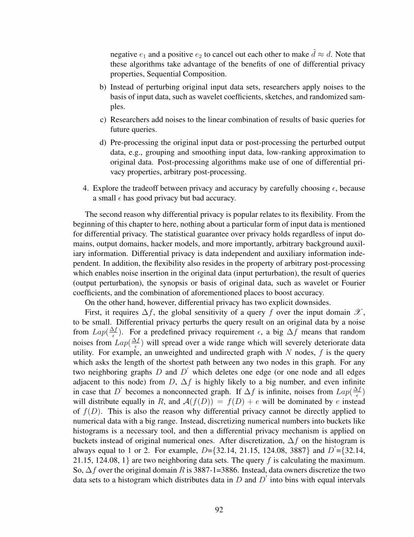
negative e1 and a positive e2 to cancel out each other to make d ≈ d. Note thatthese algorithms take advantage of the benefits of one of differential privacyproperties, Sequential Composition.

b) Instead of perturbing original input data sets, researchers apply noises to thebasis of input data, such as wavelet coefficients, sketches, and randomized sam-ples.

c) Researchers add noises to the linear combination of results of basic queries forfuture queries.

d) Pre-processing the original input data or post-processing the perturbed outputdata, e.g., grouping and smoothing input data, low-ranking approximation tooriginal data. Post-processing algorithms make use of one of differential pri-vacy properties, arbitrary post-processing.

4. Explore the tradeoff between privacy and accuracy by carefully choosing ε, becausea small ε has good privacy but bad accuracy.

The second reason why differential privacy is popular relates to its flexibility. From thebeginning of this chapter to here, nothing about a particular form of input data is mentionedfor differential privacy. The statistical guarantee over privacy holds regardless of input do-mains, output domains, hacker models, and more importantly, arbitrary background auxil-iary information. Differential privacy is data independent and auxiliary information inde-pendent. In addition, the flexibility also resides in the property of arbitrary post-processingwhich enables noise insertion in the original data (input perturbation), the result of queries(output perturbation), the synopsis or basis of original data, such as wavelet or Fouriercoefficients, and the combination of aforementioned places to boost accuracy.

On the other hand, however, differential privacy has two explicit downsides.First, it requires ∆f , the global sensitivity of a query f over the input domain X ,

to be small. Differential privacy perturbs the query result on an original data by a noisefrom Lap(∆f

ε). For a predefined privacy requirement ε, a big ∆f means that random

noises from Lap(∆fε

) will spread over a wide range which will severely deteriorate datautility. For example, an unweighted and undirected graph with N nodes, f is the querywhich asks the length of the shortest path between any two nodes in this graph. For anytwo neighboring graphs D and D

′ which deletes one edge (or one node and all edgesadjacent to this node) from D, ∆f is highly likely to a big number, and even infinitein case that D′ becomes a nonconnected graph. If ∆f is infinite, noises from Lap(∆f

ε)

will distribute equally in R, and A(f(D)) = f(D) + e will be dominated by e insteadof f(D). This is also the reason why differential privacy cannot be directly applied tonumerical data with a big range. Instead, discretizing numerical numbers into buckets likehistograms is a necessary tool, and then a differential privacy mechanism is applied onbuckets instead of original numerical ones. After discretization, ∆f on the histogram isalways equal to 1 or 2. For example, D={32.14, 21.15, 124.08, 3887} and D′={32.14,21.15, 124.08, 1} are two neighboring data sets. The query f is calculating the maximum.So, ∆f over the original domainR is 3887-1=3886. Instead, data owners discretize the twodata sets to a histogram which distributes data in D and D′ into bins with equal intervals

92

of 1000. Hence, HD=(3, 0, 1), HD′=(4, 0, 0). ∆f over the histogram is defined as ∆f =max∀D,D′∈X |f(HD)−f(H

′D)|. As a result, ∆f is 1 which is much smaller than ∆f=3886

over the original domain R and therefor significantly increases data utility.Second, differential privacy cannot protect any privacy. Its protection only covers the

presence or absence of memberships in a group. In other words, differential privacy paysattention to statistically bounded contribution of any single original data to output domains.Because the contribution of any single original data is bounded, the ability to breach thepresence or absence of any member is also limited. Differential privacy, however, is notcapable of preserving privacy beyond membership presence. For example, assume d is thenumber of smokers in Kentucky, d = d + e is the ε-differentially privatized version of d.Based on d, it is likely to guess the rough range of the original d. So, d cannot keep a goodprivacy of d’s possible range. Instead, given d, the ability to guess any person in Kentuckybeing a smoker or not is statistically bounded.

Copyright c© Lian Liu, 2015.

93

Chapter 7 A User-Perspective Accuracy Analysis of Differential Privacy

In this chapter, accuracy analysis of a differentially private query from a public user per-spective is studied. In most differential privacy applications, data owners hold originalconfidential data, and are required to fulfill a data analysis task along with a differentialprivacy parameter ε. Data owners are needed to carefully design a differential privacymechanism to achieve a satisfactory tradeoff between privacy and accuracy. Usually, dataowners could use the standard differential privacy mechanism, the Laplace Mechanism[45], to meet a predefined privacy requirement. Then, further analyses verify the accuracyof perturbed data under the Laplace Mechanism with the privacy parameter ε. If the resultof accuracy analysis is satisfied, the data owners proceed to publish it to the public. Oth-erwise, they must design a subtle differential privacy mechanism to replace the standardLaplace Mechanism to boost accuracy, or choose a new privacy parameter ε. Noted that abigger ε means worse privacy but better accuracy.

The standard Laplace Mechanism can satisfy the privacy-accuracy balance for a richbody of industrial applications, such as the demographic census [24] and healthcare [40].For privacy, the standard Laplace Mechanism can simply hold ε-differential privacy. Manypapers [75, 78, 172, 177] used the Mean Squared Error (MSE) to quantify accuracy. Forexample, the cardinality of original data D in X is N , i.e., D = {di}, i = 1, ..., N .Accuracy is considered satisfactory with respect to an upper bound Υ, if 1

N

∑Ni=1(di −

di)2 ≤ Υ. Data owners can claim that after the application of the differential privacy

mechanism, released data satisfies ε-differential privacy and Υ-accuracy.The above perspective is the point of view of data owners. But from the user’s perspec-

tive, the upper bound Υ of accuracy is not always meaningful for two reasons.First, given a theoretic upper bound of accuracy over the entire input domain, there is

no opportunity to exploit or verify it in the age of big data because there is no access to theentire input domain due to the time limitation, such as time-series sequences which will goon indefinitely, or public users are not authorized to explore the entire data set.

Second, faced with the released perturbed data, users only care about the accuracy of aportion of perturbed data, rather than the entire data set. It is necessary for biostatisticansor biomedical providers to have knowledge of the bound of utility of a subset of releaseddata prior to advanced processing [52], for example.

In Figure 7.1, for instance, a public user has only access to the green perturbed data andconsiders the following questions?

• How close is d40503 to the original data d40503?

• What is the difference between d40503 + d40506 + d40508 and the original counterpartof the corresponding original data?

• Provided that d40506 is the maximum of the six areas in the public report, what is theprobability that d40506 is still the maximum of the original data?

• Given the fact that d40506 + d40511 > d40503 + d40508, what is the probability thatd40506 + d40511 > d40503 + d40508?

94

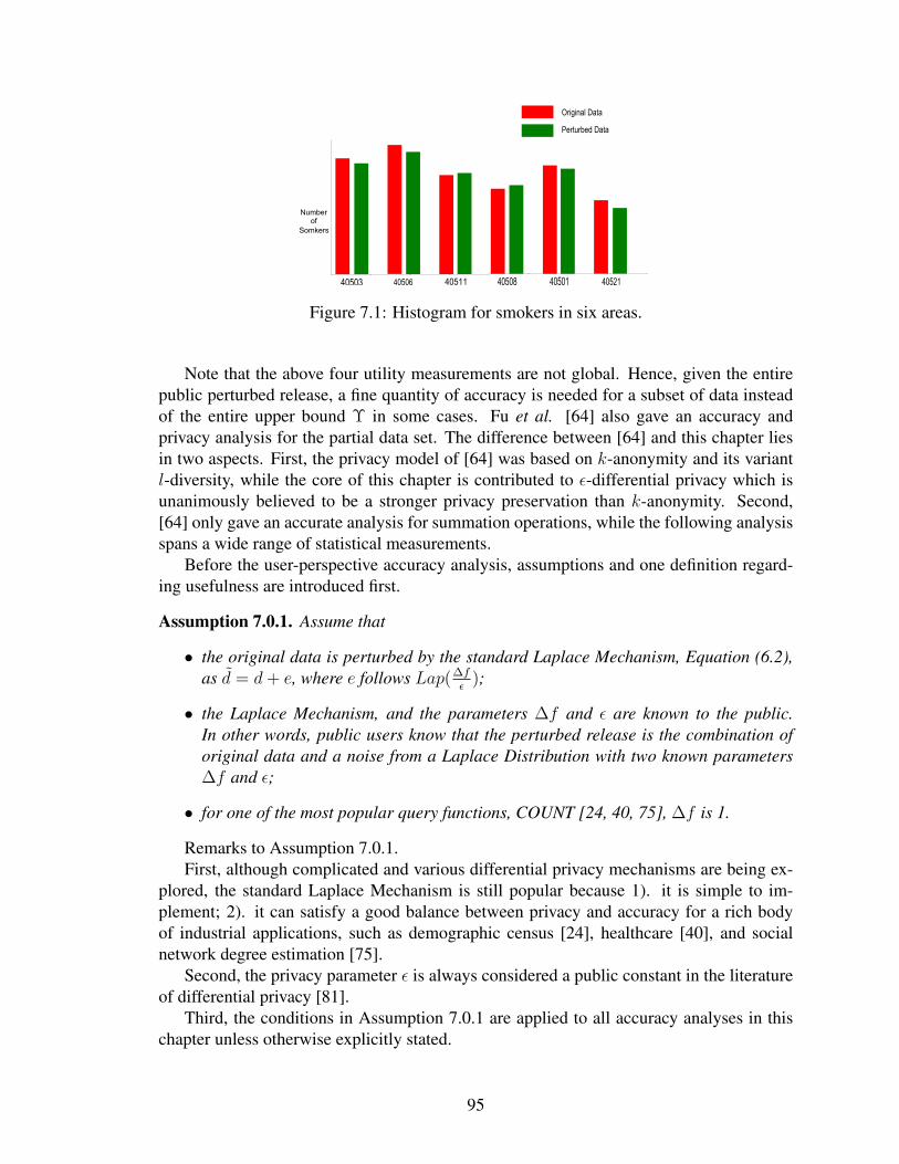
40503 40506 40511 40508 40501 40521

Original Data

Perturbed Data

Numberof

Somkers

Figure 7.1: Histogram for smokers in six areas.

Note that the above four utility measurements are not global. Hence, given the entirepublic perturbed release, a fine quantity of accuracy is needed for a subset of data insteadof the entire upper bound Υ in some cases. Fu et al. [64] also gave an accuracy andprivacy analysis for the partial data set. The difference between [64] and this chapter liesin two aspects. First, the privacy model of [64] was based on k-anonymity and its variantl-diversity, while the core of this chapter is contributed to ε-differential privacy which isunanimously believed to be a stronger privacy preservation than k-anonymity. Second,[64] only gave an accurate analysis for summation operations, while the following analysisspans a wide range of statistical measurements.

Before the user-perspective accuracy analysis, assumptions and one definition regard-ing usefulness are introduced first.

Assumption 7.0.1. Assume that

• the original data is perturbed by the standard Laplace Mechanism, Equation (6.2),as d = d+ e, where e follows Lap(∆f

ε);

• the Laplace Mechanism, and the parameters ∆f and ε are known to the public.In other words, public users know that the perturbed release is the combination oforiginal data and a noise from a Laplace Distribution with two known parameters∆f and ε;

• for one of the most popular query functions, COUNT [24, 40, 75], ∆f is 1.

Remarks to Assumption 7.0.1.First, although complicated and various differential privacy mechanisms are being ex-

plored, the standard Laplace Mechanism is still popular because 1). it is simple to im-plement; 2). it can satisfy a good balance between privacy and accuracy for a rich bodyof industrial applications, such as demographic census [24], healthcare [40], and socialnetwork degree estimation [75].

Second, the privacy parameter ε is always considered a public constant in the literatureof differential privacy [81].

Third, the conditions in Assumption 7.0.1 are applied to all accuracy analyses in thischapter unless otherwise explicitly stated.

95

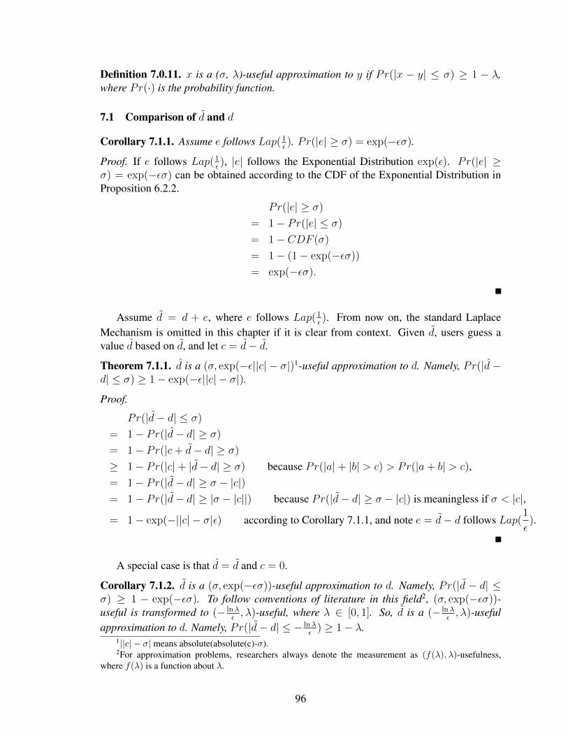
Definition 7.0.11. x is a (σ, λ)-useful approximation to y if Pr(|x − y| ≤ σ) ≥ 1 − λ,where Pr(·) is the probability function.

7.1 Comparison of d and d

Corollary 7.1.1. Assume e follows Lap(1ε). Pr(|e| ≥ σ) = exp(−εσ).

Proof. If e follows Lap(1ε), |e| follows the Exponential Distribution exp(ε). Pr(|e| ≥

σ) = exp(−εσ) can be obtained according to the CDF of the Exponential Distribution inProposition 6.2.2.

Pr(|e| ≥ σ)

= 1− Pr(|e| ≤ σ)

= 1− CDF (σ)

= 1− (1− exp(−εσ))

= exp(−εσ).

Assume d = d + e, where e follows Lap(1ε). From now on, the standard Laplace

Mechanism is omitted in this chapter if it is clear from context. Given d, users guess avalue d based on d, and let c = d− d.

Theorem 7.1.1. d is a (σ, exp(−ε||c| − σ|)1-useful approximation to d. Namely, Pr(|d −d| ≤ σ) ≥ 1− exp(−ε||c| − σ|).

Proof.

Pr(|d− d| ≤ σ)

= 1− Pr(|d− d| ≥ σ)

= 1− Pr(|c+ d− d| ≥ σ)

≥ 1− Pr(|c|+ |d− d| ≥ σ) because Pr(|a|+ |b| > c) > Pr(|a+ b| > c),= 1− Pr(|d− d| ≥ σ − |c|)= 1− Pr(|d− d| ≥ |σ − |c||) because Pr(|d− d| ≥ σ − |c|) is meaningless if σ < |c|,= 1− exp(−||c| − σ|ε) according to Corollary 7.1.1, and note e = d− d follows Lap(

1

ε).

A special case is that d = d and c = 0.

Corollary 7.1.2. d is a (σ, exp(−εσ))-useful approximation to d. Namely, Pr(|d − d| ≤σ) ≥ 1 − exp(−εσ). To follow conventions of literature in this field2, (σ, exp(−εσ))-useful is transformed to (− lnλ

ε, λ)-useful, where λ ∈ [0, 1]. So, d is a (− lnλ

ε, λ)-useful

approximation to d. Namely, Pr(|d− d| ≤ − lnλε

) ≥ 1− λ.1||c| − σ| means absolute(absolute(c)-σ).2For approximation problems, researchers always denote the measurement as (f(λ), λ)-usefulness,

where f(λ) is a function about λ.

96

According to Theorem 7.1.1 and Corollary 7.1.2, given d and the public privacy param-eter ε, it is easy to get a probability, 1− exp(−εσ), that how close is di to di.

7.2 Comparison of∑di and

∑di

Next, the difference,∑N

i=1 ei, between∑di and

∑di will be demonstrated. Note that al-

though there is superscript N in all following summation-related equations, the superscriptN can be replaced by any others, such as N

2, M (M ≤ N ), and so on. This replacement

means that all following theorems can be applied to any arbitrary subset of the entire dataset. This is accuracy analysis from a user perspective, i.e., public users only care aboutwhat users interest in.

Corollary 7.2.1. The distribution of∑N

i=1 ei is the same as∑N

i=1(−1)jiei, where ji israndomly 1 or 0 for i = 1, ..., N , and ei follows Lap(1

ε).

Corollary 7.2.1 means that for exampleN=5, e1−e2−e3+e4−e5,−e1−e2+e3−e4−e5,e1 − e2 + e3 + e4 + e5, and e1 + e2 + e3 + e4 + e5 have a same distribution. The proofof Corollary 7.2.1 is simple because Lap(1

ε) is a symmetric distribution about the y axis.

e ∈ Lap(1ε) and −e ∈ Lap(1

ε) have the same PDF (Probability Density Function). So, the

PDF of e1 + e2 is essentially the same as e1 − e2, for instance.

Theorem 7.2.1. (Theorem 6.5 in [73]3) Let E =∑N

i=1 ei, where ei follows Lap(1ε), for i

= 1, ..., N . {Pr(E ≥ −6 lnλ

ε) ≤ λ, if N < −6 lnλ,

Pr(E ≥√−6N lnλ

ε) ≤ λ, if N ≥ −6 lnλ.

(7.1)

E is symmetric about the the y axis because each element ei in E is symmetric. So |E|can be obtained as followsPr(|E| ≥ −

6 ln λ2

ε) ≤ λ, if N < −6 ln λ

2,

Pr(|E| ≥√−6N ln λ

2

ε) ≤ λ, if N ≥ −6 ln λ

2.

(7.2)

Remarks to Theorem 7.2.1. Fixing a given probability λ, the mean of E is approaching3A similar theorem was obtained as Lemma 2.8 in [27].

97

to 0 when N is close to infinite because of the following.

Pr(E ≥√−6N lnλ

ε) ≤ λ, if N →∞

Pr(E

N≥√−6N lnλ

εN) ≤ λ,

Pr(E

N≥√−6 lnλ

ε√N

) ≤ λ,

Pr(E

N≤√−6 lnλ

ε√N

) ≥ 1− λ, (7.3)

Pr( limN→∞

E

N≤ lim

N→∞

√−6 lnλ

ε√N

) ≥ 1− λ,

Pr( limN→∞

E

N≤ 0) ≥ 1− λ.

A similar result about the mean of |E| can be obtained. The result Pr(limN→∞|E|N≤ 0) ≥

1−λ is consistent with the fact of the mean of noises from Lap(1ε) being 0. Equation (7.3)

provides a detailed measurement about when the mean of E is small enough with respectto ε, λ, and N .

0 200 400 600 800 10000

0.1

0.2

0.3

0.4

0.5

0.6

0.7

0.8

0.9

Per

cent

age

N

µ=0, ǫ=0.2, error=1

Figure 7.2: Mean of Laplace noises.

Figures 7.2 and 7.3 illustrate that the means of Laplace noises are approaching 0 whenthe number of noises, N , is from 1 to 1000. When N=200, for example, this method gen-erates 200 noises from Lap( 1

0.2) in Figure 7.2, sums the 200 noises, repeats the generation

and sum processes 10000 times, and counts the percentage/ratio of the number of sums

98

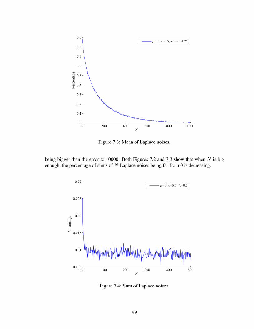
0 200 400 600 800 10000

0.1

0.2

0.3

0.4

0.5

0.6

0.7

0.8

0.9

Per

cent

age

N

µ=0, ǫ=0.5, error=0.25

Figure 7.3: Mean of Laplace noises.

being bigger than the error to 10000. Both Figures 7.2 and 7.3 show that when N is bigenough, the percentage of sums of N Laplace noises being far from 0 is decreasing.

0 100 200 300 400 5000.005

0.01

0.015

0.02

0.025

0.03

Per

cent

age

N

µ=0, ǫ=0.1, λ=0.2

Figure 7.4: Sum of Laplace noises.

99

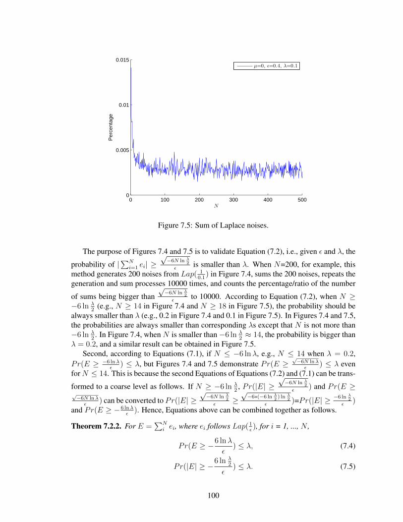
0 100 200 300 400 5000

0.005

0.01

0.015

Per

cent

age

N

µ=0, ǫ=0.4, λ=0.1

Figure 7.5: Sum of Laplace noises.

The purpose of Figures 7.4 and 7.5 is to validate Equation (7.2), i.e., given ε and λ, the

probability of |∑Ni=1 ei| ≥

√−6N ln λ

2

εis smaller than λ. When N=200, for example, this

method generates 200 noises from Lap( 10.1

) in Figure 7.4, sums the 200 noises, repeats thegeneration and sum processes 10000 times, and counts the percentage/ratio of the number

of sums being bigger than√−6N ln λ

2

εto 10000. According to Equation (7.2), when N ≥

−6 ln λ2

(e.g., N ≥ 14 in Figure 7.4 and N ≥ 18 in Figure 7.5), the probability should bealways smaller than λ (e.g., 0.2 in Figure 7.4 and 0.1 in Figure 7.5). In Figures 7.4 and 7.5,the probabilities are always smaller than corresponding λs except that N is not more than−6 ln λ

2. In Figure 7.4, when N is smaller than−6 ln λ

2≈ 14, the probability is bigger than

λ = 0.2, and a similar result can be obtained in Figure 7.5.Second, according to Equations (7.1), if N ≤ −6 lnλ, e.g., N ≤ 14 when λ = 0.2,

Pr(E ≥ −6 lnλε

) ≤ λ, but Figures 7.4 and 7.5 demonstrate Pr(E ≥√−6N lnλ

ε) ≤ λ even

forN ≤ 14. This is because the second Equations of Equations (7.2) and (7.1) can be trans-

formed to a coarse level as follows. If N ≥ −6 ln λ2, Pr(|E| ≥

√−6N ln λ

2

ε) and Pr(E ≥

√−6N lnλ

ε) can be converted to Pr(|E| ≥

√−6N ln λ

2

ε≥√−6∗(−6 ln λ

2) ln λ

2

ε)=Pr(|E| ≥ −6 ln λ

2

ε)

and Pr(E ≥ −6 lnλε

). Hence, Equations above can be combined together as follows.

Theorem 7.2.2. For E =∑N

i ei, where ei follows Lap(1ε), for i = 1, ..., N ,

Pr(E ≥ −6 lnλ

ε) ≤ λ, (7.4)

Pr(|E| ≥ −6 ln λ2

ε) ≤ λ. (7.5)

100

Although Equations (7.4) and (7.5) are coarser than the counterparts in Theorem 7.2.1,they are independent of the number of noise variables from Lap(1

ε). In the following con-

text, both Equations in Theorems 7.2.1 and 7.2.2 are needed to handle different require-ments.

Theorem 7.2.3 can be obtained as follows, by the combination of Theorem 7.2.2 andCorollary 7.2.1.

Theorem 7.2.3. Suppose E =∑N

i=1(−1)jiei, where ji=1 or 0 randomly for i = 1, ..., N ,and ei follows Lap(1

ε) for i = 1, ..., N .

Pr(E ≥ −6 lnλ

ε) ≤ λ,

Pr(|E| ≥ −6 ln λ2

ε) ≤ λ.

Next, how to determine whether∑N1

i=1 di ≥∑N2

j=1 dj given the fact∑N1

i=1 di ≥∑N2

j=1 djwill be shown.

Theorem 7.2.4. For simplicity, suppose∑N1

i=1 di ≥∑N2

j=1 dj , and let c =∑N2

j=1 dj −∑N1

i=1 di, and N = N1 +N2. It is clear that c ≤ 0.

Pr(

N1∑i=1

di ≥N2∑j=1

dj) ≥{

1− exp( cε6

), if N < −cε,1− exp(− c2ε2

6N), if N ≥ −cε. (7.6)

Proof.

Pr(

N1∑i=1

di ≥N2∑j=1

dj)

= Pr(

N1∑i=1

(di − ei) ≥N2∑j=1

(dj − ej))

= Pr(

N1∑i=1

di −N2∑j=1

dj ≥N1∑i=1

ei −N2∑j=1

ej)

= Pr(−c ≥N∑k=1

ek)

= Pr(N∑k=1

ek ≤ −c)

= 1− Pr(N∑k=1

ek ≥ −c).

Just follow Equations (7.1) of Theorem 7.2.1 and substitute −c for −6 lnλε

and√−6N lnλ

εto

figure out the probability λ. For instance, let −c = −6 lnλε

, λ = exp( cε6

) is obtained, if

101

N < −cε.

Theorem 7.2.4 quantifies the possibility of comparison of original data, and the possi-bility is only contingent on public parameters ε, N , and c.

First, looking at Equations (7.6), the smaller c is (i.e.,∑N1

i=1 di is much bigger than∑N2

j=1 dj , and note c is negative), the bigger possibility of∑N1

i=1 di ≥∑N2

j=1 dj is. It isconsistent with the common sense.

Second, the bigger ε is, the bigger possibility of∑N1

i=1 di ≥∑N2

j=1 dj is. In Figure 6.1,a big ε makes most random variables to concentrate on a narrower range around the y axisthan a small ε.

Similar to Theorem 7.2.4 which is built upon Equation (7.1), the boundary of the dif-ference between two original data can be quantified by the boundary of two perturbed datawith the aid of Equation (7.2).

Theorem 7.2.5. For simplicity, suppose∑N1

i=1 di ≥∑N2

j=1 dj , and let c =∑N2

j=1 dj −∑N1

i=1 di, and N = N1 +N2. It is clear that c ≤ 0. For ∀σ > 0,

Pr(|N1∑i=1

di −N2∑j=1

dj| ≤ σ) ≤{

1−max(1, 2 exp(− ε(σ+|c|)6

)), if N < ε(σ + |c|),1−max(1, 2 exp(− ε2(σ+|c|)2

6N)), if N ≥ ε(σ + |c|).

Proof.

Pr(|N1∑i=1

di −N2∑j=1

dj| ≤ σ)

= Pr(|N1∑i=1

(di − ei)−N2∑j=1

(dj − ej)| ≤ σ)

= Pr(|N1∑i=1

di −N2∑j=1

dj −N1∑i=1

ei +

N2∑j=1

ej| ≤ σ)

= Pr(| − c+N∑k=1

ek| ≤ σ)

≤ Pr(−|c|+ |N∑k=1

ek| ≤ σ)

≤ Pr(|N∑k=1

ek| ≤ σ + |c|)

≤ 1− Pr(|N∑k=1

ek| ≥ σ + |c|).

Similarly, follow Equations (7.2) of Theorem 7.2.1 and substitute σ + |c| for −6 ln λ2

εand√

−6N ln λ2

εto figure out the probability λ. Note that, for instance, let σ + |c| = −6 ln λ

2

ε,

102

λ = 2 exp(− ε(σ+|c|)6

) and its range is [0, 2]. But λ is a probability which should be in therange [0, 1]. So, λ is limited to max(1, 2 exp(− ε(σ+|c|)

6)).

Based on Theorem 7.2.5, observations, similar to ones from Theorem 7.2.4, can beobtained.

Given ε, N , and the difference between∑N1

i=1 di and∑N2

j=1 dj , Theorem 7.2.4 quantifiesthe possibility of

∑N1

i=1 di ≥∑N2

i=1 dj , and Theorem 7.2.5 measures the possibility of theabsolute difference between

∑N1

i=1 di and∑N2

i=j dj being no more than a threshold. In Figure7.1, knowing the perturbed (green) data, the confidence can be held that the real number ofsmokers on campus (zipcodes: 40503, 40506, and 40508) is more than the one off campus(zipcodes: 40511, 40501, and 40521), and the difference of numbers of smokers betweenon-campus and off-campus is not small.

7.3 Max, Min, Sum, and Mean

This subsection, based on ε and di, i= 1, ...,N , will show how to determine max(d1, ..., dN),min(d1, ..., dN),

∑Ni di, and mean(d1, ..., dN). The max/min estimation in a privacy pre-

serving fashion is helpful for applications in decision theory [56], game theory [70], statis-tics [150], and network topology [65].

Theorem 7.3.1. Assume ∀ dmax ≥ di, for i = 1, ..., N , and ci = di − dmax.

Pr(dmax ≥ max(d1, ..., dN)) ≥N∏i=1

f(ci, ε),

where

f(ci, ε) =

{1− exp( ciε

6), if 1 < −ciε,

1− exp(− ci2ε2

6), if 1 ≥ −ciε.

Theorem 7.3.2. Assume ∀ dmin ≤ di, for i = 1, ..., N , and ci = dmin − di.

Pr(min(d1, ..., dN) ≥ dmin) ≥N∏i=1

f(ci, ε),

where

f(ci, ε) =

{1− exp( ciε

6), if 1 < −ciε,

1− exp(− ci2ε2

6), if 1 ≥ −ciε.

The proof of Theorems 7.3.1 and 7.3.2 can be directly deduced from Theorem 7.2.4.They can help users obtain a confidence about what the max/min values of original datashould be. Based on di, i=1, ...,N , to guess the max/min values of di with a high confidenceλ, say 99%, it is just needed to do the following jobs. First, solve ci from 1− exp( ciε

6) = λ

N

and 1 − exp(− ci2ε2

12) = λ

N, and pick up any value dmax ≥ ci + di and dmin ≤ di − ci,

∀ i = 1, ..., N . Beyond this naive method, other sophisticated or adaptive methods arepromising to be explored in the future.

103

Two extensions of Theorem 7.2.1, the summation and the mean of original data, areshown next.

Theorem 7.3.3.∑N

i=1 di is a (6 ln 2

λ

ε, λ)-useful approximation forN < −6 lnλ, or (

√6N ln 2

λ

ε, λ)-

useful approximation to∑N

i=1 di when N ≥ −6 lnλ.

Theorem 7.3.4. 1N

∑Ni=1 di is a (

6 ln 2λ

Nε, λ)-useful approximation forN < −6 lnλ, or (

√6 ln 2

λ

ε√N, λ)-

useful approximation to 1N

∑Ni=1 di when N ≥ −6 lnλ.

Theorem 7.3.3 is just an extension of Equations (7.2) in Theorem 7.2.1. Accordingto Equation (7.3), Theorem 7.3.4 is easily obtained. Both theorems can give public usersa confidence about the summation and the mean of original data with the help of publicperturbed data and two known parameters N and ε.

Copyright c© Lian Liu, 2015.

104

Chapter 8 An I/O-Aware Algorithm for a Differentially Private Mean of a BinaryStream

8.1 Introduction

Collecting statistical measures from online retailers, search engines, location-based serviceproviders, social network portals brings an explosion of interest in mining stream data, inorder to have a deep understanding of valuable social and economic patterns, like diseaseoutbreaks [22], over a long term. The introduction of stream mining also fuels debatesof potential privacy leakages because tracking historical patterns uncovers more sensitiveknowledge than one-shot analysis, which will in turn potentially breach personal privacy[23, 145], and even cause casualties [62]. Therefore, privacy preserving collections andpublications of aggregated information from a stream are a necessary task.

In the age of big data, the volume of data is exploded at an exponential rate, and theability of calculation based on big data is also increased due to the development of compu-tational hardware and software infrastructures. However, this development is not advancedat the same speed between computational devices and input/output drives. The speeds ofI/O operations and network transmission cannot keep pace with the advance of memorybandwidths and CPU clock rates.

According to [128], Henry Newman provided a survey that memory bandwidths in-creased from 4.3GB/sec in 2004 to 40GB/sec in 2009 for Intel, PCI-X boosted bus band-widths from 250MB/sec in 2004 to 1GB/sec in 2010, and CPU units doubled its per-formance every 18 months under Moore’s Law. But SATA Disk performances only im-proved from 64MB/sec to 84MB/sec recently, and the total throughput of Ethernet (Wire-less 802.1g, resp.) is just 10MB/sec (54MB/sec, resp.). Because frequent I/O operations,like disk seeks and network transmissions, are expensive comparing to CPU calculationsand memory fetches, they become a bottleneck in the age of big data [85] and are worth-while paying an attention. Memcachem, an in-memory hash table which was implementedby Facebook to mitigate the performance bottleneck, supports billions of requests on tril-lions of data per second, to alleviate congestions dominated by I/O operations of data re-trievals [130]. Due to limitations of bandwidths, on the other hand, statistical measurescannot be transmitted losslessly over links of finite capacities, and only a subset of se-quences of sensor’s readings can be transported to central servers [140, 96].

In this chapter, how to release a differentially private mean of a binary stream withan I/O-awareness is studied. Briefly, the purpose of this study is to release the mean (orexpected value) of a binary stream in a differential privacy preservation way, and try tohave as less I/O operations as possible at the same time, like hard drive reading, writing,and network transmissions.

A wealth of researchers already shed light on the problem of releasing a private ag-gregation of statistical measures over streams from a variety of perspectives, like fault-tolerance [84, 28], multi-parties [29], distributed sources [63], high-dimensional domains[57], differentially private aggregations and variants pan-privacy [50, 119, 27], binarystreams [27], and streams with special properties [26, 20]. To the best of our knowledge,

105

there is little attention to be shifted to the I/O-aware private aggregation of streams.For simplicity, this preliminary study begins with an easy setting, a binary stream with

only elements 0 or 1 which is also the research target in [27]. Let S = {0, 1}N be abinary stream of the length of N , and the element Si at timestamp i be 0 or 1, and θ(t) =1t

∑ti=1 Si, where t ≤ N . Note that the length N can be extended to infinite.

The purpose of private mean publications of a binary stream is to release θ(t) instead ofthe original θ(t) in order to limit the attacker’s confidence about Si=0 or 1, ∀ i ≤ t. For I/O-awareness, I/O operations, like hard drive reading, writing, and network transmissions, aredesired to be limited. Assume reading a bit Si of the binary stream from a local storage (ahard drive) or remote resources (networks) is one time I/O operation. Because the privacypreservation algorithm is just disclosing θ(t) to the public, writing I/O operations are notin the scope of our consideration. But it is probably desired to release multiple θ(t)s fordifferent t ≤ N , and the maximum number of publications is N , i.e., the private meanhas to be published at each timestamp. To this end, sampling and approximation are tookfor granted. Simply, θ(t) or θ(t) can be approximated with the help of retrieving a certainsubset of Si. The detailed schema will be introduced in Sections 8.3 and 8.4.

8.2 Analysis of Previous Methods

Previous Privacy Preservation Releasing Model

Releasing a differentially private measure, like sum, of an binary stream has two ways.First, at timestamp i, a differentially private bit is generated in the form of Si = Si

+ ei, where ei follows a Laplace Distribution Lap(1ε). Then SUM(t)=

∑ti=1 Si, where

t ≤ N , is released to the public. The series of publications at each timestamp, (SUM(1),SUM(2), ..., SUM(N)), is ε-differentially private since each bit of the stream is involved

in one differential privacy mechanism. But at each timestamp i, SUM(i) is (√−6i ln λ

2

ε,

λ)-useful approximation to SUM(i). That is, Pr(|SUM(i) − SUM(i)| ≤√−6i ln λ

2

ε) =

Pr(|∑ij=1 ej| ≤

√−6i ln λ

2

ε) ≥ 1− λ, according to Equation (7.2) of Theorem 7.2.1.

Second, at timestamp i, a differentially private sum SUM(i) = SUM(i) + ei is di-rectly released to the public, where ei follows a Laplace Distribution Lap(1

ε). (SUM(1),

SUM(2), ..., SUM(N)), is (Nε)-differentially private since each bit of the stream is in-volved in N differential privacy mechanisms. According to the property of sequentialcomposition of differential privacy, its protection level is (Nε)-differentially private. Onthe other hand, at timestamp i, SUM(i) is (− lnλ

ε, λ)-useful approximation to SUM(i),

according to Corollary 7.1.2.It is clear that the first scheme has a high privacy because ε-privacy is better than (Nε)-

privacy, but a low accuracy since√−6i ln λ

2

εis bigger than − lnλ

ε, when i → ∞. To get a

good balance between privacy and accuracy, previous works [27, 26, 20] used a combi-nation strategy in which authors heuristically split a stream into substreams, like (0, 1, 0,1, 1, 1, 0)=((0), (1, 0, 1), (1), (1, 0)), used the first scheme to privatize each substream to

106

get multiple private intermediate results, and used the second scheme to obtain a privatesum of the intermediate results. The challenges are how to make a well-balanced splitstrategy in terms of accuracy and privacy. Until now, the known best differentially pri-vate sum publications can achieve (O(1

ε(logN)1.5 log( 1

λ)), λ)-useful approximations, i.e.,

Pr[SUM(N)−SUM(N)| ≤ O(1ε(logN)1.5 log( 1

λ))] ≥ 1−λ, while the protection is still

ε-differential privacy [27].

Limitations

The above strategy has three drawbacks as follows.First, although the accuracy complexity is O(1

ε(logN)1.5 log( 1

λ))1, the complexity of

its I/O operations is O(N). That is, it needs to scan all bits of a binary stream in onepass or more. For a long stream and a large number of online queries during the rushhour, like Facebook information retrieval infrastructure to support billions of requests ontrillions of data per second [130], the feedback of online queries will be dominated bythe time-consuming I/O operations which deteriorate user experiences. Hence, an I/O-aware privacy scheme should harvest as less data from I/O devices as possible at a cost ofsacrificing a little bit accuracy.

Second, the accuracy provided in [27] is an absolute error bound which is independentof the real sum. In other words, for two real sums, say 10 and 10, 000, the accuracy boundis the same. For a small-valued real sum, a big accuracy bound is not helpful. So, a relativeaccuracy bound is desired.

Third, the Standard Laplace Mechanism used in [27, 26, 20] cannot keep consistence.It is clear that the maximum (minimum, resp.) of the sum of a binary stream of the lengthof N is N (0, resp.). But publishing either SUM(N) � N or SUM(N) � 0 is likelyto happen in the Standard Laplace Mechanism for a binary stream. The reason why thissituation happens is because noises from Lap(1

ε) may dominate SUM if ε is big. So, the

level of privacy protection defined by ε cannot be arbitrarily strong, and there is a balancebetween accuracy and privacy if users need to keep consistent statistical measures. In theexample of a private mean of a binary stream, θ(i) should always be in [0, 1]. Anotherinconsistent problem of the Standard Laplace Mechanism used in [27, 26, 20] for a binarystream to release a private sum is SUM(i) > SUM(i + 1). In fact, for a binary stream,SUM(i) ≤ SUM(i + t), where for any t ≥ 1, always holds. A privacy preservationscheme should also keep this property. But due to a Laplace noise being probably negative,SUM(i) > SUM(i+ 1) in some cases [27, 26, 20]. For example, a binary stream is (0, 1,0, 1, 0), SUM(4) = SUM(4) + e4 = 2 + e4, and SUM(5) = SUM(5) + e5 = 2 + e5. Ife4 ≥ 0, e5 ≤ 0, and e4 ≤ |e5|, then θ(4) > θ(5). To overcome this problem, noises from anExponential Distribution are chosen instead of a Laplace Distribution. For a private meanpublication, it is not a problem, because the mean for a binary stream is not monotonous.A bit of 0 will decrease the mean and a bit of 1 will increase the mean.

1For a real output Out and a perturbed output Out, the accuracy complexity O( 1ε (logN)1.5 log( 1

λ ))

means that ∃k, for any Out and Out, |Out−Out| ≤ k 1ε (logN)1.5 log( 1

λ ).

107

8.3 Private Mean Releasing Scheme

Introduction to the private mean publication scheme with the aid of Reservoir Sampling[161] is given first in this section. Second, it will be proved that this scheme satisfiesε-differential privacy.

As said in the previous section, noises from a Laplace Distribution may ignite incon-sistency, i.e., the mean of a binary stream is below 0. Instead, random variables from anExponential Distribution will play a role in the publication of a consistent and private mean.

Although the backbone of the Exponential Distribution in differential privacy was al-ready introduced in the previous chapter, it will be re-introduced for self-contained pur-poses.

Proposition 8.3.1. [79] If a noise e comes from Lap(∆fε

), |e| followsExp( ε∆f

) whose PDF(Probability Density Function) is

PDF (e) =

{ε

∆fexp(−e ε

∆f) e ≥ 0,

0 e < 0,

and whose CDF (Cumulative Density Function) is

CDF (e) =

{1− exp(−e ε

∆f) e ≥ 0,

0 e < 0.

From Proposition 8.3.1, it is clear that any noise from Exp( ε∆f

) is non-negative.Algorithm 3 shows how to generate a differentially private bit of a binary stream.

Algorithm 3 Releasing a differentially private bit.Input: Si ∈ {0, 1} and εOutput: Si

1: Randomly generate ei from Exp(ε)2: Si = Si + ei

After Algorithm 3, it is possible that Si ≥ 1. It looks like not consistent. But thefinal intention is to release a private and consistent mean. Here, we can temporally ignoreinconsistency of individual private bits.

Next, it is needed to prove that Algorithm 3 is ε-differential privacy for individual bits.According to the introduction to preliminaries of differential privacy in the previous

chapter, the input domain X = {0, 1}, and there are just four neighboring data sets, (D ={0}, D′ = {0}), (D = {1}, D′ = {1}), (D = {1}, D′ = {0}), and (D = {0}, D′ = {1}),in this input domain for individual bits 2.

Theorem 8.3.1. Algorithm 3 generates an ε-differentially private bit of a single element ofa binary stream.

2Quick reminder: D and D′

are neighboring data sets, iff 1). D ∈ X and D′ ∈ X ; 2). max(|D −

D′ |, |D′ −D|) ≤ 1.

108

Proof. According to Definition 6.2.5, a randomized mechanismA is ε-differentially privateif, for any two neighboring data sets D and D′ and any subset S in the domain of all realnumbers,

Pr[A(f(D)) ∈ S] ≤ exp(ε)Pr[A(f(D′)) ∈ S].

Here, ∆f = 1, Si = f(D), and Si is short for A(f(D)). The privacy mechanismadds noises from an Exponential Distribution to original data to generate A(f(D)) andA(f(D

′)) for D and D′ .

Pr(t = A(f(D)))

Pr(t = A(f(D′))

=Pr(t = f(D) + e1)

Pr(t = f(D′) + e2)

=Pr(e1 = t− f(D))

Pr(e2 = t− f(D′))

=PDF (t− f(D))

PDF (t− f(D′))

=

ε∆fexp(−(t− f(D)) ε

∆f)

ε∆fexp(−(t− f(D′)) ε

∆f)

= exp((−t+ f(D) + t− f(D

′))ε

∆f)

= exp((f(D)− f(D

′))ε

∆f)

≤ exp(ε).

For a static binary array, i.e., the length is fixed and will not be increased in the future,if users would publish a differentially private mean with limited I/O operations, they canrandomly select a subset of differentially private bits generated by Algorithm 3 to approx-imate the mean. But for a binary stream, i.e., the length will be increased forever, if userswould publish a series of private means, like (θ(10), θ(26), θ(73), θ(110), θ(198), ...), dothey need to select different subsets of bits to approximate various θ(i)s? No, to approx-imate θ(26), for example, users can take advantage of subsets used by approximation toθ(10). The reuse of subsets is to reduce the burden of I/O operations.

Based on Algorithm 3, the I/O-awareness private mean publication scheme is illustratedin Algorithm 4.

In Algorithm 4, briefly, n = 2+σσ2 ln 2

λis the number of randomly selected bits to ap-

proximate the mean of St, i.e., θ(t). This approximation has an accuracy Pr(|θ(t)−θ(t)| ≤σ + 1

ε

√6σ2

2+σ) ≥ 1 − λ, where θ(t) = 1

n

∑nj=1(Sij + eij). Why n = 2+σ

σ2 ln 2λ

and

Pr(|θ(t) − θ(t)| ≤ σ + 1ε

√6σ2

2+σ) ≥ 1 − λ will be introduced in detail in next section.

Note that n is independent of the length of a binary stream, and it is only based on theaccuracy requirements, e.g., parameters σ and λ. When the length of a binary stream is

109

Algorithm 4 An I/O-awareness private mean publication.Input: S ∈ {0, 1}∞, (t1, t2, ..., tq) where each ti ≥ 1 and ti ≤ ti+1, ε > 0, σ ∈ [0, 1], and

λ ∈ [0, 1].

Output: (θ(t1), ..., θ(tq)) s.t. for each i ∈ {1, 2, ..., q}, Pr(|θ(ti)−θ(ti)| ≤ σ+ 1ε

√6σ2

2+σ) ≥

1− λ.1: Create an array W of a size of n = 2+σ

σ2 ln 2λ

in the cache2: if tq ≤ n then3: for i=1 to tq do4: Wi = Si + ei, where ei follows Exp(ε)5: if i ∈ {t1, t2, ..., tq} then6: θ(i) = 1

i

∑ik=1Wk

7: end if8: end for9: else

10: for i=1 to n do11: Wi = Si + ei, where ei follows Exp(ε)12: end for13: r = 1 and t = tr14: for i=n+ 1 to t do15: j is randomly selected between 1 and i16: if j ≤ n then17: Wj = Si + ei, where ei follows Exp(ε)18: else19: Do not read Si from the local storage or transmit it from networks20: end if21: if i = t then22: θ(i) = 1

n

∑nk=1Wk

23: r = r + 1 and t = tr24: end if25: if r > q then26: Private Mean Publication is finished and Quit27: end if28: end for29: end if

110

increased, the number of selected bits for approximation does not change if the accuracyrequirement is unchanged.

In Algorithm 4, if tq ≤ n (Lines 2 to 8), the mean does not have to be approximated.For example, to calculate θ(10), just figure out θ(10) = 1

10

∑10i=1(Si + ei).

Theorem 8.3.2. In Algorithm 4, the probability of each bit of the binary stream S ∈ {0, 1}t

to be chosen is independent and identical, and the probability is nt

=2+σ

σ2ln 2λ

t.

Proof. Consider a scenario that users would release θ(t). At timestamp i (Line 14), Algo-rithm 4 generates a random number j between 1 and i (Line 15). If j is less than n, Wj isreplaced with Si + ei (Lines 16 and 17). In fact, for all i, the probability that Si is chosento be included in W is n/i. Similarly, the probability of Wj being chosen to be replacedwith is 1/n * n/i, which can be simplified to 1/i. And after execution, each bit of S has anindependent and identical probability, i.e., n/t, of being included in W .

The reason why Algorithm 4 can limit I/O operations is threefold.First, to calculate θ(t), Algorithm 4 does not fetch all data from I/O devices (Line 19).Second, to obtain θ(t2) after the calculation of θ(t1), Algorithm 4 does not read a fresh

subset of n randomly selected bits from I/O devices. Instead, it continues updating W bychanging the range of new randomly selected bits from t1 to t2 (Line 23).

Third, because the capacity of the reservoir, the array W to store randomly selectedbits in Algorithm 4, is small and limited, users can use cache to act as the reservoir andreadings/writings can be done in the cache which are much faster than in the I/O devices.So, the I/O operations implemented in the cache will not be counted in the I/O-awarealgorithm.

Theorem 8.3.3. For any binary stream, the differential privacy mechanism A can keepconsistency, i.e., θ(i) ≥ 0, for any i.

Its proof is straightforward, because a non-negative noise from the Exponential Distri-bution will add to θ at each timestamp. On the other hand, how to impose the consistencyof θ(i) ≤ 1 for any i depends on the choice of ε and will be introduced in the next section.

Theorem 8.3.4. The series of private means (θ(t1), ..., θ(tq)) published by Algorithm 4 isε-differentially private.

Proof. We first prove each θ(ti) is ε-differentially private for example, then demonstratethis series is also ε-differential private.

For two neighboring binary streams ST and SD in the domain Sti , assume they have thesame length ti, and they have exactly the same contents but one bit. That is,

∑tij=1(STj −

SDj)2 = 1, where STj (SDj , resp.) is the bit of ST (SD, resp.) at timestamp j. Suppose

the only different bit is at timestamp k.According to Definition 6.2.5, Algorithm 4 is ε-differentially private for θ(ti) if, for any

two neighboring data sets ST and SD and any subset S in the domain of all real numbers,

Pr[θ(ST(ti)) ∈ S] ≤ exp(ε)Pr[θ(SD(ti)) ∈ S]. (8.1)

111

Here, ∆f = 1, and θ(ST(ti)) is the private mean for the binary stream ST at timestamp ti.Because Algorithm 4 is an approximated scheme which will randomly select bits to

calculate θ(ti). STk and SDk, i.e., the only different bits, have two options. They areselected by Algorithm 4, or not.

If STk and SDk are not selected, θ(ST(ti)) = θ(SD(ti)) according to Algorithm 4. So,Equation (8.1) is satisfied.

Consider the scenario that STk and SDk are selected. For simplicity, assume the firstn bits are selected to approximate, and STk and SDk are the last bits, i.e., k = n. Then,∑n−1

j=1 (STj + ej) =∑n−1

q=1 (SDq + eq), according to Algorithm 4.

Pr(y = θ(ST(ti)))

Pr(y = θ(SD(ti)))

=Pr(y =

∑nj=1(STj + ej))

Pr(y =∑n

q=1(SDq + eq))

=Pr(y =

∑n−1j=1 (STj + ej) + STk + ek)

Pr(y =∑n−1

q=1 (SDq + eq) + SDk + e′k)

=Pr(ek = y −∑n−1

j=1 (STj + ej)− STk)Pr(e

′k = y −∑n−1

q=1 (SDq + eq)− SDk)

=PDF (y −∑n−1

j=1 (STj + ej)− STk))PDF (y −∑n−1

q=1 (STq + eq)− SDk))

=

ε∆fexp(−(y −∑n−1

j=1 (STj + ej)− STk) ε∆f

)

ε∆fexp(−(y −∑n−1

q=1 (STq + eq)− SDk)ε

∆f)

= exp((STk − SDk)ε

∆f)

≤ exp(ε).

So, Equation (8.1) is satisfied too.

8.4 The Chernoff Bounds

This section will present why Pr(|θ(t)− θ(t)| ≤ σ+ 1ε

√6σ2

2+σ) ≥ 1−λ when n = 2+σ

σ2 ln 2λ

samples are chosen to approximation in Algorithm 4. The reason lies in the backgroundof the Chernoff Bounds and its application. Armed with the help of the Chernoff Bounds,approximation of measures, like the mean, of a binary stream in a differential privacy waywill be given later.

Briefly speaking, the Chernoff Bound, proposed by Herman Chernoff, presents an ex-ponentially decreasing bound on tail distributions of sums of independent random vari-ables. One of its popular applications is probably in sampling and polling because its vari-ant can approximate the distribution of a population with a given property, e.g., approvalof a candidate, by the subset of all populations.

112

Proposition 8.4.1. [121] The Chernoff Bound. Let X1, ..., XN be independent ran-dom variables within the range of [0, 1], X =

∑Ni=1 Xi, and µ = Expected(X) =∑N

i=1Expected(Xi). Note that here X1, ..., XN are not required to follow an identicaldistribution.

Then for any τ > 0,

Pr(X ≥ (1 + τ)µ) ≤ exp(− τ 2

2 + τµ),

P r(X ≤ (1− τ)µ) ≤ exp(−τ2

2µ).

Proposition 8.4.2. The Two-sided Chernoff Bound. Follow the setting of Proposition8.4.1, and let τ ∈ [0, 1],

Pr(|X − µ| ≥ τµ) ≤ 2 exp(− τ 2

2 + τµ). (8.2)

Proof. {Pr(X ≥ (1 + τ)µ) ≤ exp(− τ2

2+τµ),

P r(X ≤ (1− τ)µ) ≤ exp(− τ2

2µ).

For τ ∈ [0, 1],

⇒{Pr(X ≥ (1 + τ)µ) ≤ exp(− τ2

2+τµ),

P r(X ≤ (1− τ)µ) ≤ exp(− τ2

2µ) ≤ exp(− τ2

2+τµ).

Sum up the two inequalities above to get Equation (8.2).

The released mean is a differentially private one, θ(i) = 1i

∑ij=1(Sj+ej) = 1

i

∑ij=1 Sj+∑i

j=1 ej , which includes two parts, the sum of the original binary stream and the sum ofadded Exponential noises. How to approximate the first part,

∑ij=1 Sj , is given first with

the help of the Chernoff Bound in the next subsection.

Approximation to∑i

j=1 Sj

Inspired by the lecture note [157], we consider the scenario of a binary stream of the lengthof N . Assume a percentage of all bits in the binary stream being 1 is p ∈ [0, 1]. p is theaccurate mean of a binary stream and is the research target in this chapter. From anotherperspective, p also presents the probability of a bit in the stream being to 1. Next, we willshow how to estimate p with the help of a subset of the entire stream.

S1, ..., SN are independent, and Nθ(N) =∑N

i=1 Si since θ(N) is the real mean andNθ(N) is the sum of the binary stream by the multiplication of mean and the number ofbits. It follows a Bernoulli distribution with N and p, i.e., Nθ(N) ∼ Bernoulli(N , p),whose expectation, µ, is Np. According to Equation (8.2) of Proposition 8.4.2, for any

113

τ ∈ [0, 1],

Pr(|Nθ(N)− µ| ≥ τµ) ≤ 2 exp(− τ 2

2 + τµ),

P r(|Nθ(N)−Np| ≥ τNp) ≤ 2 exp(− τ 2

2 + τNp),

P r(|θ(N)− p| ≥ τp) ≤ 2 exp(− τ 2

2 + τNp),

P r(|θ(N)− p| ≥ τp) ≤ 2 exp(− τ 2p2

2p+ τpN). (8.3)

For p ∈ [0, 1], 2 exp(− τ2p2

2p+τpN) ≤ 2 exp(− τ2p2

2+τpN). Hence, Equation (8.3) can be trans-

formed to

Pr(|θ(N)− p| ≥ τp) ≤ 2 exp(− τ 2p2

2 + τpN). (8.4)

Let σ = τp, Equation (8.4) is

Pr(|θ(N)− p| ≥ σ) ≤ 2 exp(− σ2

2 + σN). (8.5)

Theorem 8.4.1. If Si1 , Si2 , ..., Sin , where n ≥ 2+σσ2 ln 2

λ, are randomly picked and θ(n) =

1n

∑nj=1 Sij , then Pr(|θ(n)− p| ≤ σ) ≥ 1− λ, where p is the accurate mean (or expected

value) of the binary stream in the form of p = 1N

∑Nj=1 Sj . Armed with n bits of a length-N

binary stream, θ(n) is an approximation to p.

Proof. According to Equation (8.5), Pr(|θ(N)−p| ≤ σ) ≥ 1−2 exp(− σ2

2+σN). To satisfy

Pr(|θ(N)−p| ≤ σ) ≥ 1−λ, 2 exp(− σ2

2+σN) has to be smaller than λ. Solve the inequality

2 exp(− σ2

2+σN) ≤ λ to get the result N ≥ 2+σ

σ2 ln 2λ

. Namely, only 2+σσ2 ln 2

λbits can achieve

the (σ, λ)-useful approximation to p. In the following content, n is the number of randomlyselected bits for approximation, i.e., n ≥ 2+σ

σ2 ln 2λ

.

Note that n ≤ N in this chapter, and n bits of the binary stream are picked up to approx-imate the statistical measures of the entire length-N stream. Hence, θ(n) = 1

n

∑nj=1 Sij is

(σ, λ)-useful approximation to p = 1N

∑Nj=1 Sj , where n ≥ 2+σ

σ2 ln 2λ

. The biggest advan-tage of Theorem 8.4.1 lies in the fact that the number of bits, n ≥ 2+σ

σ2 ln 2λ

, chosen to makean accurate approximation to the entire population is independent of N , the length of thebinary stream. In other words, for a given usefulness metric with two predefined param-eters σ and λ, the number of chosen bits to approximate the entire population is almostirrelevant to the increasing length of streams in real time. This property of irrelevancy isessentially helpful for extreme long and even infinite streams.

Proposition 8.4.1, Proposition 8.4.2, and Theorem 8.4.1 are related to the original bi-nary stream. Next, we will show how to approximate the sum of added Exponential noises.

114

Table 8.1: Ranges of exponential noises.

ε [0, ln(1000ε)]0.01 [0, 2.3]0.1 [0, 4.7]0.2 [0, 5.3]0.5 [0, 6.3]1 [0, 6.9]10 [0, 9.2]

Approximation to∑i

j=1 ej

If the privacy parameter ε is known, there is no need to approximate∑i

j=1 ej because it canbe bounded by Theorem 7.2.1. So, this subsection mainly focuses on how to approximate∑i

j=1 ej by the Chernoff Bound when ε is unknown.One of conditions of the Chernoff Bound is Xi ∈ [0, 1]. Noises from the Exponen-

tial Distribution is in [0, +∞]. Noises from a standard Exponential Distribution can betruncated to be fit in with the Chernoff Bound.

According to the CDF (Cumulative Density Function) of the Exponential Distributionin Proposition 8.3.1,

CDF (e) = 1− exp(−eε), for e ≥ 0,

99.9% noises from this distribution will fall in [0, ln(1000ε)]. Some ranges about [0,ln(1000ε)] are shown in Table 8.4.

Based on the above table, it is highly likely that 99.9% noises from the ExponentialDistribution are not more than 10. Note that in differential privacy, it is unlikely to letthe privacy parameter ε be too big, because even if ε=2, according to Definition 6.2.5,Pr[A(f(D))∈S]

Pr[A(f(D′ ))∈S]≤ exp(ε), the privacy level will decrease at the rate of exp(ε) = exp(2) ≈

7.4. Most applications [81] of differential privacy adopted ε ∈ [0, 1].Despite an unknown ε, ei from an Exponential Distribution spans the range [0, 10]

with a probability of at least 99.9%. So ei10

is in [0, 1]. Expected( ei10

) = 110ε

sinceExpected(ei) = 1

εwhere ei follows an Exponential Distribution Exp(ε).

Assume e1, e2, ..., eN follow an Exponential Distribution Exp(ε) with an unknownparameter ε, and E =

∑Ni=1 ei. According to Equation (8.2) in Proposition 8.4.2, the

115

following holds

Pr(|E10− 1

10ε| ≥ τ

10ε) ≤ 2 exp(− τ 2

2 + τ

1

10ε),

P r(|E − 1

ε| ≥ τ

ε) ≤ 2 exp(− τ 2

2 + τ

1

10ε),

P r(|EN− 1

Nε| ≥ τ

Nε) ≤ 2 exp(− τ 2

2 + τ

1

10ε).

Let ε′=

1

Nε,

Pr(|EN− ε′| ≥ τε

′) ≤ 2 exp(− Nε

′τ 2

20 + 10τ),

P r(|EN− ε′| ≥ τε

′) ≤ 2 exp(− Nτ 2(ε

′)2

20ε′ + 10ε′τ).

If ε ≥ 1

N, ε′ ≤ 1,

Pr(|EN− ε′| ≥ τε

′) ≤ 2 exp(− Nτ 2(ε

′)2

20 + 10ε′τ).

Let σ = τε′,

Pr(|EN− ε′ | ≥ σ) ≤ 2 exp(− Nσ2

20 + 10σ). (8.6)

Based on Equation (8.6), the number of noises from an Exponential Distribution withan unknown parameter ε to approximate the entire population can be obtained.

Theorem 8.4.2. If ei1 , ei2 , ..., ein , where n ≥ 20+10σσ2 ln 2

λ, are randomly picked, Pr(|

∑nj=1 eijn−

1Nε| ≤ σ) ≥ 1−λ, where 1

εis the accurate mean (or expected value) of Exponential noises

of the entire population.

The proof is similar to the one of Theorem 8.4.1. The number of selected noises toapproximate all Exponential random variables is also independent of ε and N , the lengthof a binary stream. It is clear that the number of selected noises, n ≥ 20+10σ

σ2 ln 2λ

, toapproximate all Exponential random variables is 10 times of the one, n ≥ 2+σ

σ2 ln 2λ

, toapproximate the original binary stream.

In detail, for a binary stream S = {0, 1}N , an ε-differentially private sum is iθ(i) =∑ij=1(Sj +ej), where Sj is the bit of the stream at timestamp j and ej follows an Exponen-

tial Distribution with the parameter ε. Randomly selected n ≥ 2+σσ2 ln 2

λbits of the binary

stream can approximate∑i

j=1 Sj with a high confidence. On the other hand, randomlyselected n ≥ 20+10σ

σ2 ln 2λ

Exponential random variables can approximate∑i

j=1 ej with ahigh confidence. Combined the two numbers together, n ≥ 20+10σ

σ2 ln 2λ

randomly selectedSj = Sj + ej can approximate θ(i).

One reason why we would shed light on the situation of the privacy parameter ε beingunknown is that according to Theorem 8.4.2, n ≥ 20+10σ

σ2 ln 2λ

is independent of ε. Theproperty of independence on ε means that a variety of privacy protection (i.e., different ε)

116

can be applied to various bits of a binary stream, given a fact that different bits do not havethe same privacy requirement.

Analysis of I/O Operations and Accuracy

In Section 8.3, the ε-differential privacy for Algorithm 4 is already proved. This sectionwill show the complexity of I/O operations and accuracy.

Theorem 8.4.3. The complexity of I/O operations for Algorithm 4 is O(1), i.e., a constantindependent of the length of a binary stream.

Theorem 8.4.3 is clear because Algorithm 4 just reads n ≥ 2+σσ2 ln 2

λbits from local

storages or networks. And n is only in relation to σ and λ, which are parameters to controlaccuracy.

Theorem 8.4.4. For a binary stream S, assume n ≥ 20+10σσ2 ln 2

λbits, Si1 , ..., Sin , from

this stream St are randomly selected, θ(t) = 1t

∑tj=1 Sj , and θ(t) = 1

n

∑nj=1(Sij + ej),

where ej follows an Exponential Distribution with the parameter ε, then Pr(|θ(t)−θ(t)| ≤σ + 1

ε

√6σ2

2+σ) ≥ 1− λ.

Copyright c© Lian Liu, 2015.

117

Chapter 9 Security Information Retrieval on Private Data Sets

9.1 Introduction

With the development of public awareness of privacy protection, privacy preservationshould not only expand to the underlying data sets, but also cover information users pro-vide to the Internet interface. Because such information probably reveals confidential andidentifiable messages pertaining to religious affiliations, sexual orientations, political opin-ions, personal identities, and to name a few. For example, it was reported by the WallStreet Journal that Staples, Inc., presented different prices for various customers based ontheir location-based information, such as zipcodes or Location-Based Identities (GPS) [42].Customers close to Staples’ competitors tend to receive a discounted price.

Privacy Preserving Data Mining, like differential privacy [19, 24, 40, 45, 46, 47, 48,50, 81, 102, 113, 119, 120, 146, 149, 172, 177, 178, 100, 99, 101], mainly focuses on theproblem that the underlying data sets are sensitive. On the other hand, Private InformationRetrieval (PIR) [67, 133] entitles users to search patterns from a server who holds a publicdata set without revealing the information users provide to the server.

In this chapter, the problem of launching an information retrieval between users andservers with protection on both sides is studied. Although PIR can also be extended to thisproblem, compared to differential privacy, it has two downsides. First, PIR basically ex-ploits homomorphic encryption techniques which are computationally expensive and needa lot of communication budgets between users and servers. Second, PIR is an ad-hocscheme. Namely, a PIR algorithm is compatible with one task, but may be not good forother purposes. The reason lies in the nature of encryption techniques. In contrast, differen-tial privacy is a perturbation-based technique whose space complexity is almost a constant[27] and its run time is linear with the cardinality of the input. Because differentially pri-vate perturbation is able to preserve main statistical properties of data sets, and the secureoutputs are capable of benefiting multiple tasks simultaneously, discussed in Chapter 6.

Problem Formalization and A Naive Solution

Conceptually, suppose the server holds an original data set x, like the histogram in Figure7.1, and the client keeps an original query y, like a series of keywords. For simplicity,assume x and y are two numerical vectors with the same length. If not, we could pad zerosto the short one. The purpose of the information retrieval is to compute xTy. For example,in Figure 7.1, x = (167, 182, 143, 135, 151, 109)T , y = (1, 1, 0, 1, 0, 0), xTy means thetotal number of smokers around the campus of the University of Kentucky.

To protect personal privacy, like smoking addictions, to avoid potential employmentand health insurance discrimination, the histogram needs to be safeguarded before pub-lication. An ε-differentially private histogram, represented by x, is generated. The sameprinciple is also applied to the query y, which will be perturbed to y in a differential privacyway. Based on y, malicious ones can infer that the querist is likely to have a relationship

118

with the University of Kentucky, such as living around the campus, an employee of theuniversity, prospective students dreaming of this institution, etc.

The client sends y to the server by communication channels, and the server will returnxT y to the client, instead of xTy.

So, the first task is analyzing |xTy − xT y|, which is hoped to be as small as possible.A naive solution is generating x = x + ex and y = y + ey, where ex and ey follow

Lap(1ε), by the Standard Laplace Mechanism. Theorem 6.2.1 proves that the naive solution

can make x and y ε-differentially private.In the histogram example, for instance, x=(172.13, 178.98, 125.03, 139.87, 140.10,

97.87), y=(0.285, 1.875, 0.951, 2.871, -0.91, 0.123).A problem of the naive solution is surfaced as far as communication costs, measured

by the size of data to be transmitted, are concerned. In most cases, the original query y isa sparse vector. But after a differential privacy process, y becomes a dense one. In the ageof big data, compared to y, y means that the client has to send more data to the server. So,it is not a good choice.

A naive improvement is that the client only transports a subset of y by k-anonymity,like yk=(0.285, 1.875, 0.951, 2.871, 0, 0), where k=4, instead of the entire y.

There is also a drawback. Based on yk= (0.285, 1.875, 0.951, 2.871, 0, 0), for example,it is clear that the original keywords are existed in the first four areas and the latter twoareas are not in the scope of interests. If the client chooses yk = (0, 1.875, 0, 2.871, -0.91,0), for instance, xT y will definitely lose desired patterns, like the number of smokers in thefirst area. This problem happens because each keyword only exists in one element of y.

Hence, the second task is making the communication cost, measured by the size of y orits variant, as small as possible.

9.2 Accuracy Analysis of the Naive Solution

Without consideration of communication complexity, the naive solution demonstrated inthe previous section is sending the entire y to the server which will in turn compute xT y.In this section, the bound of |xTy − xT y| is analyzed from the theoretic and user pointsof view. Simply, the theoretic bound of |xTy − xT y| is shown in Theorem 9.2.1, whileTheorem 9.2.3 presents the bound from the user perspective. What are the theoretic anduser perspectives meaning will be explained in this section in detail. All notations usedin this chapter are briefly summarized in Table 9.1. The details of these notations will beintroduced when necessary.

Theorem 9.2.1. Expected(|xTy−xT y|) = 0. That is,Expected(xTy) = Expected(xT y),where Expected() is the expected value.

119

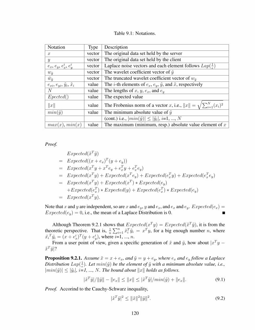
Table 9.1: Notations.

Notation Type Descriptionx vector The original data set held by the servery vector The original data set held by the clientex, ey, eix, eiy vector Laplace noise vectors and each element follows Lap(1

ε)

wy vector The wavelet coefficient vector of ywy vector The truncated wavelet coefficient vector of wyexi, eyi, yi, xi value The i-th elements of ex, ey, y, and x, respectivelyN value The lengths of x, y, ex, and eyEpected() value The expected value

‖x‖ value The Frobenius norm of a vector x, i.e., ‖x‖ =√∑N

i=1(xi)2

min(y) value The minimum absolute value of y(cont.) i.e., |min(y)| ≤ |yi|, i=1, ..., N

max(x), min(x) value The maximum (minimum, resp.) absolute value element of x

Proof.

Expected(xT y)

= Expected((x+ ex)T (y + ey))

= Expected(xTy + xT ey + eTx y + eTx ey)

= Expected(xTy) + Expected(xT ey) + Expected(eTx y) + Expected(eTx ey)

= Expected(xTy) + Expected(xT ) ∗ Expected(ey)

+Expected(eTx ) ∗ Expected(y) + Expected(eTx ) ∗ Expected(ey)

= Expected(xTy).

Note that x and y are independent, so are x and ey, y and ex, and ex and ey. Expected(ex) =Expected(ey) = 0, i.e., the mean of a Laplace Distribution is 0.

Although Theorem 9.2.1 shows that Expected(xTy) = Expected(xT y), it is from thetheoretic perspective. That is, 1

n

∑ni=1 x

Ti yi = xTy, for a big enough number n, where

xiT yi = (x+ eix)

T (y + eiy), where i=1, ..., n.From a user point of view, given a specific generation of x and y, how about |xTy −

xT y|?Proposition 9.2.1. Assume x = x+ ex, and y = y + ey, where ex and ey follow a LaplaceDistribution Lap(1

ε). Let min(y) be the element of y with a minimum absolute value, i.e.,

|min(y)| ≤ |yi|, i=1, ..., N . The bound about ‖x‖ holds as follows.

|xT y|/‖y‖ − ‖ex‖ ≤ ‖x‖ ≤ |xT y|/min(y) + ‖ex‖. (9.1)

Proof. Accorind to the Cauchy-Schwarz inequality,

|xT y|2 ≤ ‖x‖2‖y‖2. (9.2)

120

From Equation (9.2),

‖x+ ex‖ = ‖x‖‖x‖+ ‖ex‖ ≥ ‖x‖

≥ |xT y|‖y‖

‖x‖ ≥ |xT y|‖y| − ‖ex‖.

Similarly, an upper bound about ‖x‖ can be obtained.

‖ (min(y), ...,min(y))︸ ︷︷ ︸N

x‖ ≤ |xT y|

|min(y)|‖x‖ ≤ |xT y|‖x‖ ≤ |xT y|/|min(y)|. (9.3)

‖x+ ex‖ = ‖x‖‖x‖ − ‖ex‖ ≤ ‖x‖

‖x‖ ≤ ‖x‖+ ‖ex‖. (9.4)

Combine Equations (9.3) and (9.4),

‖x‖ ≤ |xT y|/|min(y)|+ ‖ex‖.

Note that y, min(y), y, and ey are known to the client. Because xT y will be returnedback to the client, xT y is also known to the client. But the client does not know ‖ex‖ in thebound. The following Proposition is to solve this problem.

Proposition 9.2.2. Expected(r2) = 2ε2

, where r comes from Lap(1ε).

Proof. Because r follows Lap(1ε), |r| comes from an Exponential Distribution Exp(ε) and

its PDF (Probability Density Function) is{ε exp(−rε) r ≥ 0,0 r < 0.

(9.5)

121

Because r2 only changes the quantity and does not alter a PDF, the PDF of r2 is thesame as Equation (9.5). The expected value of r2 is

Expected(r2) =

∫ ∞0

r2ε exp(−rε)dr

= −∫ ∞

0

r2d(exp(−rε))

= −[r2 exp(−rε)|∞0 −∫ ∞

0

exp(−rε)d(r2)]

=

∫ ∞0

exp(−rε)d(r2)

= 2

∫ ∞0

r exp(−rε)dr

= −2

ε

∫ ∞0

r ∗ (−ε exp(−rε))dr

= −2

ε

∫ ∞0

rd(exp(−rε))

= −2

ε[r exp(−rε)|∞0 −

∫ ∞0

exp(−rε)dr]

=2

ε

∫ ∞0

exp(−rε)dr

= − 2

ε2

∫ ∞0

−ε exp(−rε)dr

= − 2

ε2

∫ ∞0

exp(−rε)d(−rε)

= − 2

ε2exp(−rε)|∞0

=2

ε2.

In Equation (9.1), ‖ex‖ =√∑N

i=1 e2xi, where exi follows a Laplace DistributionLap(1

ε).

Because the length of ex isN , whenN is a big number, limN→∞1N

∑Ni=1(exi)

2=Expected((exi)2),

according to Equation (7.3). So ‖ex‖ ≈√

2N/ε, when 2/ε2 = Expected((exi)2), accord-

ing to Proposition 9.2.2.So, Proposition 9.2.1 is modified as follows.

Theorem 9.2.2. Given x = x + ex, and y = y + ey, where ex and ey follow a LaplaceDistribution Lap(1

ε), the bound about ‖x‖ is hold as follows.

|xT y|/‖y‖ −√

2N/ε ≤ ‖x‖ ≤ |xT y|/|min(y)|+√

2N/ε. (9.6)

Theorem 9.2.3. For specific ex and ey,|xT y−xT y||xT y| ≤ ‖ey‖

max(y)+

√2Nε‖y‖

max(y)(|xT y|/|min(y)|+√

2N/ε),

where all individual items on the right side are known to the client.

122

Proof.

|xT y − xTy||xTy| =

|xTy + xT ey + eTx y + eTx ey − xTy||xTy|

=|xT ey + eTx y + eTx ey|

|xTy|

=|xT ey + eTx (y + ey)|

|xTy|

≤ |xT ey|+ |eTx y||xTy|

≤ ‖x‖ ∗ ‖ey‖+ ‖ex‖ ∗ ‖y‖|xTy|

≤ ‖x‖ ∗ ‖ey‖+√

2Nε‖y‖

max(y)‖x‖

≤ ‖ey‖max(y)

+

√2Nε‖y‖

max(y)‖x‖Substitute the upper bound in Equation (9.6) for ‖x‖,

≤ ‖ey‖max(y)

+

√2Nε‖y‖

max(y)(|xT y|/|min(y)|+√

2N/ε). (9.7)

In Equation (9.7), all individual items on the right are known to the client.

9.3 Wavelet Transformation of y

Transmission of the y or its variant should take communication costs into account in the ageof big data. As said in the introduction section of this chapter, a k-anonymized subset of yis not a good choice since either it will lose information of keywords or unearth potentialmemberships of original keywords.

Instead, wavelet sparsification scheme is proposed to save the communication costwhile maintain a desired accuracy in term of |xT y − xTy|. In this section, a basic back-ground of 1D discrete wavelet decomposition will be given first. Second, its advantageswill be explained in the security information retrieval on a private data set.

One example of 1D discrete Haar wavelet decomposition is shown in Figure 9.1. Thenumbers in blue boxes are the original data set before decomposition, and the ones includedin red boxes are wavelet coefficients. For an original vector with the length of N , thereare totally log2N levels of decomposition. For a numerical vector y, assume its waveletcoefficient vector is wy. In Figure 9.1, y=(16, 9, 11, 8, 23, 15, 10, 15), and wy=(38, -10, 4,6, 5, 2, 6, -4).

The basic procedures of 1D Haar wavelet decomposition are as follows.The first level, wydi/2e = yi+yi+1√

2and wy(di/2e+N/2) = yi−yi+1√

2, where i=1, 3, 5, ..., N /2,

di/2e is the ceiling function of i/2, and wydi/2e is the di/2e-th element of wy.

123

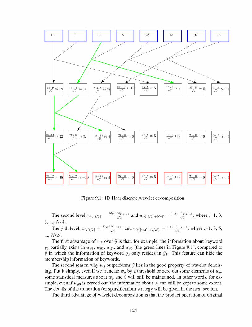
16 9 11 8 23 15 10 15

11+8√2

≈ 13 23+15√2

≈ 2716+9√2

≈ 1810+15√

2≈ 18 16−9√

2≈ 5 11−8√

2≈ 2 23−15√

2≈ 6 10−15√

2≈ −4

27+18√2

≈ 32 18−13√2

≈ 418+13√2

≈ 2216−9√

2≈ 5 11−8√

2≈ 2 23−15√

2≈ 6 10−15√

2≈ −427−18√

2≈ 6

22−32√2

≈ −10 18−13√2

≈ 422+32√2

≈ 3816−9√

2≈ 5 11−8√

2≈ 2 23−15√

2≈ 6 10−15√

2≈ −427−18√

2≈ 6

Figure 9.1: 1D Haar discrete wavelet decomposition.

The second level, wydi/2e =wyi+wy(i+1)√

2and wy(di/2e+N/4) =

wyi−wy(i+1)√2

, where i=1, 3,5, ..., N/4.

The j-th level, wydi/2e =wyi+wy(i+1)√

2and wy(di/2e+N/2j) =

wyi−wy(i+1)√2

, where i=1, 3, 5,..., N /2j .

The first advantage of wy over y is that, for example, the information about keywordy3 partially exists in wy1, wy2, wy3, and wy6 (the green lines in Figure 9.1), compared toy in which the information of keyword y3 only resides in y3. This feature can hide themembership information of keywords.

The second reason why wy outperforms y lies in the good property of wavelet denois-ing. Put it simply, even if we truncate wy by a threshold or zero out some elements of wy,some statistical measures about wy and y will still be maintained. In other words, for ex-ample, even if wy3 is zeroed out, the information about y3 can still be kept to some extent.The details of the truncation (or sparsification) strategy will be given in the next section.

The third advantage of wavelet decomposition is that the product operation of original

124

vectors can be replaced by the multiplication of wavelet coefficient vectors of x and y.

Theorem 9.3.1. Assume wx and wy are the 1D Haar wavelet coefficient vectors of x andy, and they have the same length. The following equation holds.

xT y = wTxwy.

Proof. For 1D Haar wavelet decomposition, the transformation can be presented in a ma-trix form as wx = HN ∗ x, where HN is an N ∗N (where log2N = dlog2Ne) matrix withfollowing elements [176]:

H1l = 1/√N, where l=1, ..., N,

for k ≥ 2, k = 2p + q, where 1 ≤ q ≤ 2p − 1, and 1 ≤ p ≤ N − 1,

akl =

2p−N

2 , if q2n−p ≤ l < (q + 1/2)2n−p,

−2p−N

2 , if (q + 1/2)2n−p ≤ l < (q + 1)2n−p,

0, otherwise.

For example,

H4 =

∣∣∣∣∣∣∣∣0.5 0.5 0.5 0.50.5 0.5 −0.5 −0.5√

22−√

22

0 0

0 0√

22

−√

22

∣∣∣∣∣∣∣∣ .So, HN is an invertible matrix, H−1

N = HTN , and HT

NHN = I .

wTxwy = (HN ∗ x)T (HN ∗ y)

= xT ∗HTN ∗HN ∗ y

= xT y.

Other 1D discrete wavelet decomposition techniques by various bases, like Daubechies,just involve more elements each time and have different summation and difference coeffi-cients, like

√2 in Haar. Readers can refer to [25, 60] for a comprehensive understanding

about the discrete wavelet decomposition. In other words, the server and the client donot have to use a same 1D wavelet decomposition. If they take different wavelet bases,Theorem 9.3.1 just changes to xT y = C(wTxwy). Here C is a diagonal-like (diagonal orblock-diagonal) matrix which is equal to the product of H1

N and H2N , where H1

N is thetransformed matrix of the one basis and H2

N is the other one. This chapter just considers asituation in which both sides use the same Haar basis for simplicity, but the algorithm andtheorems can be extended to the products of different wavelet bases.

Because of Theorem 9.3.1, only theorems and operations on wavelet coefficient vectorsare discussed in the following contents, instead of ones on x and y.

125

9.4 Sparsification Strategy for wy

The purpose of a sparsification strategy for wy is threefold.First, it can save communication costs. Second, it can keep the main statistical prop-

erties of y because of the nature of wavelet denoising. Third, it can keep the privacy ofinformation the client would provide to the server.

Input :yǫ-differentially privatize:

y → y

Wavelet Decomposition:

y → wy

Sparsification:

wy → wy

Output: wy

The Server

Figure 9.2: The workflow of the publication.

The entire workflow of the publication of an ε-differentially private query compati-ble with a limited communication cost is shown in Figure 9.2. Finally, the output wy tothe server should be like in the form of wy=(wy1, 0, ..., 0, wy32, 0, ..., 0, wy105, 0, ...,0, wy274, 0, ..., 0), for instance. Note that if y is ε-differentially private, wy and wy arealso ε-differentially private since wy and wy are calculated based on y. Differential pri-vacy has a property about arbitrary post-processing, i.e., any post-processed results fromε-differentially private variables are also ε-differentially private.

The accurate result of an information retrieval is xTy, and a secure information re-trieval on a private data set returns xT y which is transformed to wTxwy (according to The-orem 9.3.1) after the wavelet decomposition. The accurate bound |x

T y−xT y||xT y| is changed to

|xT y−wTx wy ||xT y| . Based on Theorem 9.3.1, |x

T y−xT y||xT y| = |x

T y−wTx wy ||xT y| . It is meaning that the wavelet

decomposition will keep the exactly same accurate bound, compared to xT y.In the previous section, the wavelet decomposition is already demonstrated. The strat-

egy for sparsification or truncation will be presented in this section.The wavelet sparsification is credited to wavelet denoising in which the big absolute

value coefficients hold most information existed in the original signal. So, the backbone is

126

how to maintain big absolute value coefficients. Remaining coefficients are dismissed byzeroing out.

A body of wavelet denoising techniques take the k biggest absolute value coefficients[38]. Others denoise w in a truncated manner [168], i.e., wi = wi, if |wi| ≥ η; otherwise,wi = 0, where η is a predefined threshold parameter. In some cases it is the mean of w orits variant, like the double or the half of the mean. In the age of big data, the method inthe first category is not desired, because finding the k biggest absolute value coefficientsof wy is a top-k algorithm whose time complexity is O(N log k) and I/O complexity ismuch higher than O(N log k). In the second category of wavelet denoising, the easy wayto know the mean is scanning all elements in the vector in one pass. So the time and I/Ocomplexities are O(N).

According to Theorems 8.4.1 and 8.4.2, a mean estimator can significantly reduce thetime and I/O complexities from O(N) to O(1) with acceptable accuracy. When the lengthof the vector is big in the age of big data, this estimator can save a lot time which is probablydominated by calculations and/or I/O operations.

The sparsification strategy for wy is as follows.

wyi =

{wyi if |wyi| ≥ η,

0 otherwise,

where η = 1n

∑nq=1 wyjq , n ≥ max(wy)

2+σσ2 ln 2

λ, and wyjq , q=1, .., n, are randomly selected

elements from wy.In the sparsification strategy, max(wy) is the element of wy with the maximum ab-

solute value. In practical cases, it can be approximated based on the nature of a waveletdecomposition. The first element of wy is the mean of y, and the second one, wy2, is thedifference between the mean of the first half y and the one of the second half. max(wy)can be approximated from whichever has a big absolute value.

Although wy1 is the mean of y, η is the mean of wy. Therefore, they are different andwy1 cannot be used to approximate η.

An accuracy bound between η and the true mean of wy can be built in a similar way toTheorems 8.4.1 and 8.4.2.

Theorem 9.4.1. If wyj1 , wyj2 , ..., wyjn , where n ≥ max(wy)2+σσ2 ln 2

λ, are randomly picked

and η = 1n

∑nq=1wyjq , then Pr(|η − 1

N

∑Ni=1wyi| ≤ σ) ≥ 1− λ.

The proof of Theorem 9.4.1 is like the one of Theorems 8.4.1 and 8.4.2. Clearly, theestimation of η has a time complexity O(1), compared to O(N) in the case of calculatingan accurate mean.

Copyright c© Lian Liu, 2015.

127

Chapter 10 Future Works

Future works can be implemented along the lines of differential privacy on large-scale datamanagement, e.g., differential privacy for small-valued numbers, e.g., 1.02 and -3.73, andverification of differential privacy. Simply, big data analysts should get used to the inte-gration of heterogeneous data, including small-valued numbers, from multiple sources. Toenhance privacy on heterogeneous data, it is necessary to pay attention to differential pri-vacy for small-valued numbers. On the other hand, with the increasing transmission of bigdata between warehouses and end-users, data corruption probably also compromises pri-vacy. In such a case, verification of differential privacy for massive data is worth exploring.

10.1 Differential Privacy for Small-Valued Numbers

Big data implicitly means a smorgasbord of heterogeneous forms, representations (e.g.,diverse health data [122]), sources, domains (e.g., real or complex domains [63]), and soon.

Differential privacy is not well compatible with the small-valued numbers, however. Adetailed discussion to touch the problem of differential privacy on small-valued numberscould be found in Chapter 6.2 of the survey [34], but it did not present a solution. Fu etal. [64] also gave a private mechanism for small sums, but their model was based on k-anonymity and its variant l-diversity. Sarathy et al. [148] and Xiao et al. [167] noticedthis problem too. Sarathy et al. [148] showed that differential privacy mechanisms ona small size of samples can result in substantial errors. Xiao et al. [167] proposed anadaptive noise injection algorithm to tackle the mixture of small- valued and big-valuednumbers in order to get a good overall accuracy. The difference between the proposalpresented in this section and the one in [167] is that [167] was dedicated to reducing theoverall errors which are caused by both small-valued and big-valued numbers. But theprivacy mechanism which generates a good overall accuracy cannot always guarantee agood accuracy for only small-valued numbers since big numbers may dominate the overallaccuracy. Hence, we only focus on the accuracy of differential privacy mechanism forpurely small-valued numbers in this section.

Assume a number of original data fall in the range [−c, c], where c > 0, and the dataowner would apply an ε-differential privacy mechanism on these data. The CDF (Cumula-tive Density Function) of a Laplace Distribution Lap(1

ε) is

CDF (x) =

{0.5 exp(xε) if x < 0,1− 0.5 exp(−xε) if x ≥ 0.

128

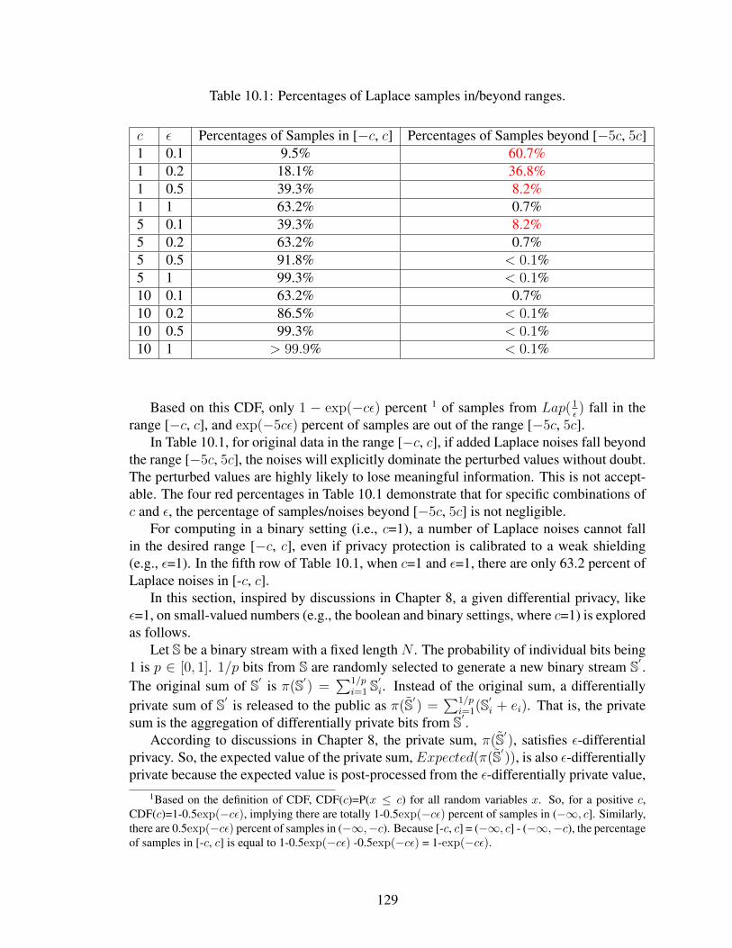
Table 10.1: Percentages of Laplace samples in/beyond ranges.

c ε Percentages of Samples in [−c, c] Percentages of Samples beyond [−5c, 5c]1 0.1 9.5% 60.7%1 0.2 18.1% 36.8%1 0.5 39.3% 8.2%1 1 63.2% 0.7%5 0.1 39.3% 8.2%5 0.2 63.2% 0.7%5 0.5 91.8% < 0.1%5 1 99.3% < 0.1%10 0.1 63.2% 0.7%10 0.2 86.5% < 0.1%10 0.5 99.3% < 0.1%10 1 > 99.9% < 0.1%

Based on this CDF, only 1 − exp(−cε) percent 1 of samples from Lap(1ε) fall in the

range [−c, c], and exp(−5cε) percent of samples are out of the range [−5c, 5c].In Table 10.1, for original data in the range [−c, c], if added Laplace noises fall beyond

the range [−5c, 5c], the noises will explicitly dominate the perturbed values without doubt.The perturbed values are highly likely to lose meaningful information. This is not accept-able. The four red percentages in Table 10.1 demonstrate that for specific combinations ofc and ε, the percentage of samples/noises beyond [−5c, 5c] is not negligible.

For computing in a binary setting (i.e., c=1), a number of Laplace noises cannot fallin the desired range [−c, c], even if privacy protection is calibrated to a weak shielding(e.g., ε=1). In the fifth row of Table 10.1, when c=1 and ε=1, there are only 63.2 percent ofLaplace noises in [-c, c].

In this section, inspired by discussions in Chapter 8, a given differential privacy, likeε=1, on small-valued numbers (e.g., the boolean and binary settings, where c=1) is exploredas follows.

Let S be a binary stream with a fixed length N . The probability of individual bits being1 is p ∈ [0, 1]. 1/p bits from S are randomly selected to generate a new binary stream S′ .The original sum of S′ is π(S′) =

∑1/pi=1 S

′i. Instead of the original sum, a differentially

private sum of S′ is released to the public as π(S′) =∑1/p

i=1(S′i + ei). That is, the privatesum is the aggregation of differentially private bits from S′ .

According to discussions in Chapter 8, the private sum, π(S′), satisfies ε-differentialprivacy. So, the expected value of the private sum, Expected(π(S′)), is also ε-differentiallyprivate because the expected value is post-processed from the ε-differentially private value,

1Based on the definition of CDF, CDF(c)=P(x ≤ c) for all random variables x. So, for a positive c,CDF(c)=1-0.5exp(−cε), implying there are totally 1-0.5exp(−cε) percent of samples in (−∞, c]. Similarly,there are 0.5exp(−cε) percent of samples in (−∞,−c). Because [-c, c] = (−∞, c] - (−∞,−c), the percentageof samples in [-c, c] is equal to 1-0.5exp(−cε) -0.5exp(−cε) = 1-exp(−cε).

129

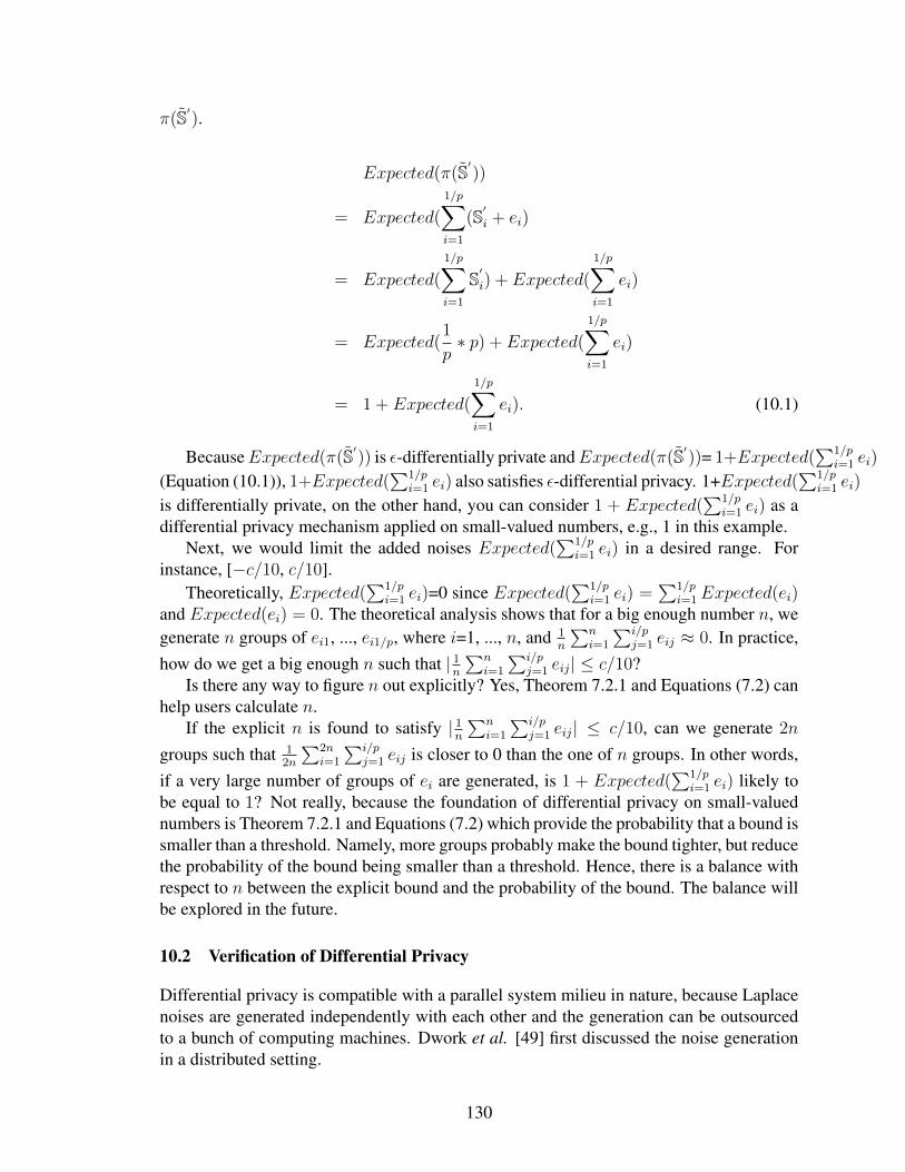
π(S′).

Expected(π(S′))

= Expected(

1/p∑i=1

(S′i + ei)

= Expected(

1/p∑i=1

S′i) + Expected(

1/p∑i=1

ei)

= Expected(1

p∗ p) + Expected(

1/p∑i=1

ei)

= 1 + Expected(

1/p∑i=1

ei). (10.1)

BecauseExpected(π(S′)) is ε-differentially private andExpected(π(S′))= 1+Expected(∑1/p

i=1 ei)

(Equation (10.1)), 1+Expected(∑1/p

i=1 ei) also satisfies ε-differential privacy. 1+Expected(∑1/p

i=1 ei)

is differentially private, on the other hand, you can consider 1 + Expected(∑1/p

i=1 ei) as adifferential privacy mechanism applied on small-valued numbers, e.g., 1 in this example.

Next, we would limit the added noises Expected(∑1/p

i=1 ei) in a desired range. Forinstance, [−c/10, c/10].

Theoretically, Expected(∑1/p

i=1 ei)=0 since Expected(∑1/p

i=1 ei) =∑1/p

i=1Expected(ei)and Expected(ei) = 0. The theoretical analysis shows that for a big enough number n, wegenerate n groups of ei1, ..., ei1/p, where i=1, ..., n, and 1

n

∑ni=1

∑i/pj=1 eij ≈ 0. In practice,

how do we get a big enough n such that | 1n

∑ni=1

∑i/pj=1 eij| ≤ c/10?

Is there any way to figure n out explicitly? Yes, Theorem 7.2.1 and Equations (7.2) canhelp users calculate n.

If the explicit n is found to satisfy | 1n

∑ni=1

∑i/pj=1 eij| ≤ c/10, can we generate 2n

groups such that 12n

∑2ni=1

∑i/pj=1 eij is closer to 0 than the one of n groups. In other words,

if a very large number of groups of ei are generated, is 1 + Expected(∑1/p

i=1 ei) likely tobe equal to 1? Not really, because the foundation of differential privacy on small-valuednumbers is Theorem 7.2.1 and Equations (7.2) which provide the probability that a bound issmaller than a threshold. Namely, more groups probably make the bound tighter, but reducethe probability of the bound being smaller than a threshold. Hence, there is a balance withrespect to n between the explicit bound and the probability of the bound. The balance willbe explored in the future.

10.2 Verification of Differential Privacy

Differential privacy is compatible with a parallel system milieu in nature, because Laplacenoises are generated independently with each other and the generation can be outsourcedto a bunch of computing machines. Dwork et al. [49] first discussed the noise generationin a distributed setting.

130

Instead of the parallel generation of Laplace noises, verification of differential privacyfor massive data will be studied in the age of big data.

Suppose there exists an HBC (honest-but-curious) middleware (middleware in shorthereafter) between the private data publisher and the public. The middleware can only seethe released data, d, and it has no access to the original sensitive data, d. It serves as averifier to confirm that the released data, d, is really ε-differentially private. If not, thereleased data will be discarded by the middleware and it will inform the data publisherto regenerate and resend the privatized data once again. Otherwise, the middleware willforward the released data to the public. Here, the middleware is honest but curious. Thatis, it will honestly report the result of verification, but it is eager to know the originalconfidential data, d. The reasons why the released data is not compatible with ε-differentialprivacy are twofold. First, the data publisher does not follow the rules of differential privacyon purpose or unintentionally. Second, the released data is polluted during the transmission,like signal loss due to long distance and the photoelectric effect. In the era of big data,with the increasing quantity of data to be collected, stored, analyzed, and transmitted, theprobability that data pollution or corruption happen is also growing.

Before the introduction to the skeleton of verification, we would answer one question.How about if the middleware maliciously changes d to violate ε-differential privacy or if dwill be also polluted in the process of transmissions between the middleware and the public.The question is equivalent to alternative ones. What is the difference between pollutionscaused by the server and the middleware? What is the difference between pollutions thathappened in the transmissions before and after the middleware?

If the middleware verifies differential privacy successfully, differential privacy will bekept even if the middleware maliciously changes anything or the released data is pollutedin the transmission from the middleware to the public. The reason is as follows. When thedata received by the middleware is ε-differentially private, any post-processing operations,like malicious alterations by the middleware and pollutions in the transmission between themiddleware and the public, on the private data cannot change its privacy property. In otherwords, any manipulation operated by the server is based on the original data, so intentionalor unintentional alternations may violate differential privacy, whereas any manipulationoperated by the middleware is based on the private data (if verification is successful), andthese alternations will keep the privacy since post-processing cannot change differentialprivacy.

There are two ways to verify whether published data is compatible with ε-differentialprivacy.

First, the middleware strictly verifies whether the published data follows the definitionof differential privacy in Definition 6.2.5. Namely, to verify the released data A(f(D)),the middleware has to find all neighboring data sets to D and all possible subsets S ∈ R,and verify whether the following holds or not.

Pr[A(f(D)) ∈ S] ≤ exp(ε)Pr[A(f(D′)) ∈ S].

This verification strategy is the safest yet most impractical solution. Because the mid-dleware has no idea about the original data set D, it has no way to enumerate all neigh-boring data sets of D. Even if D is known to it by a fully homomorphic encryption, the

131

verification process will be extremely computationally expensive since the middleware hasto enumerate all possible neighboring data sets.

Przydatek et al. [138] was testing if a sum aggregation is polluted or not by approxima-tion theory. The sum in [138] has nothing to do with any given distribution. In contrast, ε-differential privacy implicitly includes noises generated from a Laplace distribution whichcould be harnessed to refine the verification.

Hence, we move to the second verification strategy in which the middleware adaptsa private goodness of fit test for the Laplace noises contained in the released data by theKolmogorov-Smirnov test, a nonparametric test for one probability distribution.

Briefly, for n identically and independently distributed (iid) observations e1, ..., en, theempirical distribution function Fn(x) is defined as

Fn(x) =1

n

n∑i=1

Iei≤x,

where Iei≤x is the indicator function, and it is 1 if ei ≤ x, and 0 otherwise.Let D be the Kolmogorov-Smirnov statistic for a given probability distribution with the

Cumulative Distribution Function CDF(x).

D = supx|Fn(x)− CDF (x)|,

where supx is the supremum of distances.After obtaining D, the middleware can compare D with critical values in the Kolmogorov-Smirnov

Table to know if the n variables follow a given distribution. The details of goodness of fittests of Laplace distributions can be found in [139].

From the brief introduction to the Kolmogorov-Smirnov test, we can know that the keypoint is the knowledge of all n noises, e.g., e1, ..., en. But the server only sends d1, ..., dnto the middleware and di = di + ei. The middleware has no idea about the explicit valuesof ei, i=1, ..., n.

So, in the future, cryptographic protocols and non-cryptographic approximations areworthwhile trying to solve this problem without revealing explicit ei to the middleware.

Copyright c© Lian Liu, 2015.

132

Bibliography

[1] European Parliament: DIRECTIVE 2009/72/EC (2009).

[2] Kentucky QuickFacts from the US Census Bureau.http://quickfacts.census.gov/qfd/states/21000.html.

[3] Standard for Privacy of Individually Identifiable Health Information. Federal regis-ter, 66(40), 2001. http://www.hhs.gov/ocr/hipaa/finalmaster.html

[4] A. Acquisti, and R. Gross. Privacy Risks for Mining Online Social Networks. InNSF Symposium on Next Generation of Data Mining and Cyber-Enabled Discoveryfor Innovation (NGDM 2007), Baltimore, MD, October 2007.

[5] C. C. Aggarwal. On Randomization, Public Information and the Curse of Dimen-sionality. In Proceedings of the 23rd International Conference on Data Engineering(ICDE 2007), Istanbul, Turkey, April, 2007.

[6] D. Aggarwal, and C. C. Aggarwal. On the Design and Quantification of PrivacyPreserving Data Mining Algorithms. The 21st ACM SIGACT-SIGMOD-SIGARTSymposium on Principles of Database Systems, Madison, Wisconsin, June, 2002.

[7] C. C. Aggarwal, and P. S. Yu. Privacy-Preserving Data Mining: Models and Al-gorithms, Chapter 6: A Survey of Randomization Methods for Privacy-PreservingData Mining. Springer, July, 2008.

[8] R. Agrawal, R. Srikant, and D. Thomas. Privacy-Preserving Data Mining. ACMSIGMOD Record, 29(2): 439-450, 2000.

[9] L. Dall’ Asta, A. Barrat, M. Barthelemy, and A. Vespignani. Vulnerability ofWeighted Networks. Journal of Statistical Mechanics: Theory and Experiment 2006,no. 04 (2006): P04006.

[10] A. Asuncion, and D. J. Newman. UCI Machine Learning Repository. Depart-ment of Information and Computer Science, University of California, Irvine, CA.http://www.ics.uci.edu/∼mlearn/MLRepository.html, 2007.

[11] Y. Azar, A. Fiat, A. Karlin, F. Mcsherry, and J. Saia. Spectral Analysis of Data. InProceedings of The 33rd Symposium on Theory of Computing, ACM, pp. 619-626,New York, NY, 2001.

[12] L. Backstrom, C. Dwork, and J. Kleinberg. Wherefore Art Thou R3579X?Anonymized Social Networks, Hidden Patterns, and Structural Steganography. InProceedings of the 16th International Conference on World Wide Web, Alberta,Canada, pp. 181-190, 2007.

133

[13] L. Backstrom, D. Huttenlocher, J. Kleinberg, and X. Lan. Group Formation in LargeSocial Networks: Membership, Growth, and Evolution. In Proceedings of the 12thACM SIGKDD International Conference on Knowledge Discovery and Data Min-ing, Philadelphia, PA, pp. 44-54, 2006.

[14] S. Bapna, and A. Gangopadhyay. A Wavelet-Based Approach to Preserve Privacyfor Classification Mining. Decision Sciences Journal, 37(4):623-642, 2006.

[15] J. Baumes, M. Goldberg, M. Magdon-Ismail, and A. Wallace. Discovering HiddenGroups in Communication Networks. In Proceedings of the 2nd NSF/NIJ Sympo-sium on Intelligence and Security Informatics, Tucson, Arizona, pp. 378-389, June2004.

[16] Omar Benjelloun, Hector Garcia-Molina, David Menestrina, Qi Su, Steven EuijongWhang, and Jennifer Widom. Swoosh: A Generic Approach to Entity Resolution.The VLDB Journal, vol. 18, no. 1, pp. 255-276, Jan. 2009.

[17] M. W. Berry, Z. Drmac, and E. R. Jessup. Matrix, Vector Space, and InformationRetrieval. SIAM Review, 41: 335-362, 1999.

[18] Mikhail Bilenko, Raymond Mooney, William Cohen, Pradeep Ravikumar, andStephen Fienberg. Adaptive Name Matching in Information Integration. IEEE In-telligent Systems, vol. 18, no. 5, pp. 16-23, 2003.

[19] Jeremiah Blocki, Avrim Blum, Anupam Datta, and Or Sheffet. The Johnson-Lindenstrauss Transform Itself Preserves Differential Privacy. In Proceedings of the2012 IEEE 53rd Annual Symposium on Foundations of Computer Science (FOCS’12), Pages 410-419, IEEE Computer Society, Washington, DC, USA, 2012.

[20] Jean Bolot, Nadia Fawaz, S. Muthukrishnan, Aleksandar Nikolov, and Nina Taft.Private Decayed Sum Estimation under Continual Observation. arXiv preprintarXiv:1108.6123, 2011.

[21] R. B. Boppana. Eigenvalues and Graph Bisection: an Average-Case Analysis. InProceedings of the 28th Annual FOCS, pp. 280-285, Los Angeles, CA, 1987.

[22] Scott H Burton, Kesler W Tanner, Christophe G Giraud-Carrier, Joshua H West, andMichael D Barnes. ”Right Time, Right Place”: Health Communication on Twitter:Value and Accuracy of Location Information. Journal of Medical Internet Research,14(6), 2012.

[23] J. A. Calandrino, A. Kilzer, A. Narayanan, E. W. Felten, and V. Shmatilov. ”YouMight Also Like: ” Privacy Risks of Collaborative Filtering. In 2011 IEEE Sympo-sium on Security and Privacy (SP2011), pp. 231-246, Orkland, CA, 2011.

[24] A. Casteigts, M. -H. Chomienne, L. Bouchard, and G. -V. Jourdan. Differential Pri-vacy in Tripartite Interaction: A Case Study with Linguistic Minorities in Canada.DPM 2012 and SETOP 2012, LNCS 7731, 75-88, 2013.

134

[25] Kaushik Chakrabarti, Minos Garofalakis, Rajeev Rastogi, and Kyuseok Shim. Ap-proximate Query Processing Using Wavelets. The International Journal on VeryLarge Data Bases, vol. 10, no. 2-3, pp. 199-223, 2001.

[26] T. -H. Chan, Mingfei Li, Elaine Shi, and Wenchang Xu. Differentially Private Con-tinual Monitoring of Heavy Hitters from Distributed Streams. In Privacy EnhancingTechnologies, pp. 140-159, Springer Berlin Heidelberg, 2012.

[27] T. -H. Hubert Chan, Elaine Shi, and Dawn Song. Private and Continual Release ofStatistics. ACM Transactions on Information and System Security (TISSEC), vol:14, issue: 3, November 2011.

[28] T. -H. Hubert Chan, Elaine Shi, and Dawn Song. Privacy-Preserving Stream Aggre-gation with Fault Tolerance. Financial Cryptography and Data Security, pp. 200-214,Springer Berlin Heidelberg, 2012.

[29] T. -H. Chan, Elaine Shi, and Dawn Song. Optimal Lower Bound for DifferentiallyPrivate Multi-Party Aggregation. In Algorithms-ESA 2012, pp. 277-288. SpringerBerlin Heidelberg, 2012.

[30] F. C. Chang. Inversion of a Perturbed Matrix. Applied Mathematics Letters, 19:169-173, 2006.

[31] K. Chen, and L. Liu. Privacy Preserving Data Classification with Rotation Pertur-bation. In Proceedings of the 5th IEEE International Conference on Data Mining(ICDM 2005), pp. 589-592, Houston, Texas, 2005.

[32] K. Chen, G. Sun, and L. Liu. Towards Attack-Resilient Geometric Data Perturbation.In Proceedings of the 2007 SIAM International Conference on Data Mining (SDM2007), pp. 78-89, Minneapolis, MN, 2007.

[33] C. Clifton, M. Kantarcioglu, J. Vaidya, X. Lin, and M. Zhu. Tools for Privacy Pre-serving Distributed Data Mining. ACM SIGKDD Explorations, 4(2):1-7, 2003.

[34] Chris Clifton, and Tamir Tassa. On Syntactic Anonymity and Differential Privacy.Transactions on Data Privacy 6, no. 2 (2013): 161-183.

[35] R. Coifman, Y. Meyer, and V. Wickerhauser. Wavelet Analysis and Signal Process-ing. Wavelets and Their Applications, Edited by M. B. Ruskai, Jones, and BartlettPublishers, Sudbury, MA, 1991.

[36] T. H. Cormen, C. E. Leiserson, and R. L. Rivest. Introduction to Algorithms. MITPress, 1990.

[37] G. Cormode, D. Srivastava, T. Yu, and Q. Zhang. Anonymizing Bipartite Graph DataUsing Safe Groupings. In Proceedings of VLDB 2008, pp. 833-844, Auckland, NewZealand, Aug 23-28, 2008.

135

[38] Graham Cormode, Minos Garofalakis, and Dimitris Sacharidis. Fast ApproximateWavelet Tracking on Streams. In Advances in Database Technology-EDBT 2006,pp. 4-22. Springer Berlin Heidelberg, 2006.

[39] L. Cranor. Special Issue on Internet Privacy. Communications of the ACM, 42(2):28-38, 1999.

[40] Fida K. Dankar, and Khaled El Emam. Practicing Differential Privacy in HealthCare: A Review. Transactions On Data Privacy, vol: 5, pages 35-67, 2013.

[41] G. F. Davis, M. Yoo, and W. E. Baker. The Small World of the American CorporateElite, 1982-2001. Strategic Organization, 1(3): 301-326, 2003.

[42] Jennifer Valentino-DeVries, Jeremy Singer-Vine, and AshkanSoltani. Websites Vary Prices, Deals Based on Users’ In-formation. The Wall Street Journal, December 24, 2012.http://online.wsj.com/news/articles/SB10001424127887323777204578189391813881534

[43] Romain Dillet. Nest Uses Its Data To Turn Electric Utilities Into Cash Cows.TechCrunch, April 18, 2014. http://techcrunch.com/2014/04/18/nest-uses-its-data-to-turn-electric-utilities-into-cash-cows/

[44] D. Donoho. Nonlinear Wavelet Methods for Recovery of Signals, Densities andSpectra from Indirect and Noisy Data. In Proceedings of Symposia in Applied Math-ematics, American Mathematical Society, 47:173-205, 1993.

[45] Cynthia Dwork. Differential Privacy. In the 33rd International Colloquium on Au-tomata, Languages and Programming, Part II (ICALP 2006), Springer Verlag,Venice, Italy, July 2006.

[46] Cynthia Dwork. The Differential Privacy Frontier. In Proceedings of 6th Theory ofCryptography Conference, TCC 2009, Springer Verlag, San Francisco, CA, March2009.

[47] Cynthia Dwork. A Firm Foundation for Private Data Analysis. In Communicationsof the ACM, 54(1): 86-95, 2011.January 2011.

[48] Cynthia Dwork, and Adam Smith. Differential Privacy for Statistics: What WeKnow and What We Want to Learn. Journal of Privacy and Confidentiality, 1(2):2,2010.

[49] Cynthia Dwork, Krishnaram Kenthapadi, Frank McSherry, Ilya Mironov, and MoniNaor. Our Data, Ourselves: Privacy via Distributed Noise Generation. In EURO-CRYPT, pages 486-503, 2006.

[50] Cynthia Dwork, Moni Naor, Toniann Pitassi, and Guy N. Rothblum. DifferentialPrivacy under Continual Observation. In STOC ’10: In Proceedings of the 42ndACM Symposium on Theory of Computing, Cambridge, MA, June 2010.

136

[51] Cynthia Dwork, Moni Naor, Toniann Pitassi, Guy N. Rothblum, and SergeyYekhanin. Pan-Private Streaming Algorithms. In Proceedings of the First Sympo-sium on Innovations in Computer Science (ICS 2010), Tsinghua University Press,January 2010.

[52] K. E. Emam, F. K. Dankar, R. Issa, E. Jonker, D. Amyot, E. Cogo, J. -P. Corriveau,M. Walker, S. Chowdhury, R. Vaillancourt, T. Roffey, and J. Bottomley. A Glob-ally Optimal K-Anonymity Method for the De-Identification of Health Information.Journal of the American Medical Informatics Association, 16:670-682, 2009.

[53] Z. Erkin, Z. J. R. Troncoso-Pastoriza, R. L. Lagendijk, and F. Perez-Gonzalez.Privacy-Preserving Data Aggregation in Smart Metering Systems. IEEE Signal Pro-cessing Magazine, Volume: 30, Issue: 2, Pages: 75-86, 2013.

[54] A. Evfimievski. Randomization in Privacy Preserving Data Mining. ACM SIGKDDExplorations Newsletter, 4(2):43-48, 2002.

[55] A. Evfimievski, J. Gehrke, and R. Srikant. Limiting Privacy Breaches in PrivacyPreserving Data Mining. In Proceedings of PODS 2003, pp. 211-222, San Diego,CA, 2003.

[56] Alexandre Evfimievskia, Ramakrishnan Srikantb, Rakesh Agrawalb, and JohannesGehrke. Privacy Preserving Mining of Association Rules. Information Systems, Vol-ume 29, Issue 4, June 2004, Pages 343-364.

[57] Liyue Fan, Li Xiong, and Vaidy Sunderam. Differentially Private Multi-DimensionalTime Series Release for Traffic Monitoring. In Data and Applications Security andPrivacy XXVII, pp. 33-48. Springer Berlin Heidelberg, 2013.

[58] K. Faust, and S. Wasserman. Social Network Analysis: Methods and Applications.Cambridge University Press, New York, NY, 1994.

[59] I. R. Fischhoff, S. R. Sundaresan, J. Cordingley, H. M. Larkin, M. J. Sellier, andD. I. Rubenstein. Social Relationships and Reproductive State Influence LeadershipRoles in Movements of Plains Zebra, Equus Burchellii. Animal Behaviour, 73(5):825-831, 2007.

[60] Patrick Van Fleet. Discrete Wavelet Transformations: An Elementary Approach withApplications. John Wiley & Sons, 2011.

[61] L. C. Freeman, and S. C. Freeman. A Semi-Visible College: Structural Effects on aSocial Networks Group. Henderson, M.M., and McNaughton, M.J. (eds.) ElectronicCommunication: Technology and Impacts Boulder, CO: Westview Press, pp. 77-85,1980.

[62] Zoe Fox. Did Social Media Over-Sharing Lead to a Chinese Teen’s Death? Mash-able, Jan 24, 2013. http://mashable.com/2013/01/24/chinese-teen-death-weibo-social-media/

137

[63] Arik Friedman, Izchak Sharfman, Daniel Keren, and Assaf Schuster. Privacy-Preserving Distributed Stream Monitoring. In the 2014 Network and DistributedSystem Security (NDSS) Symposium, February 23-26, 2014, San Diego, Califor-nia.

[64] Ada Wai-Chee Fu, Ke Wang, Raymond Chi-Wing Wong, Jia Wang, and MinhaoJiang. Small Sum Privacy and Large Sum Utility in Data Publishing. Journal ofBiomedical Informatics, 2014, to appear.

[65] D. R. Fulkerson, and Gary C. Harding. Maximizing the Minimum Source-Sink PathSubject to a Budget Constraint. Mathematical Programming, Volume 13, Issue 1, pp116-118, 1977.

[66] S. R. Ganta, S. P. Kasiviswanathan, and A. Smith. Composition Attacks and Auxil-iary Information in Data Privacy. In Proceeding of the 14th ACM SIGKDD Interna-tional Conference (KDD’08), Las Vagas, August 2008.

[67] William Gasarch. A Survey on Private Information Retrieval. In Bulletin of theEATCS. 2004.

[68] A. Ghosh, T. Roughgarden, and M. Sundararajan. Universally Utility-MaximizingPrivacy Mechanisms. SIAM Journal on Computing 41, no. 6 (2012): 1673-1693.

[69] G. H. Golub, and C. F. Van Loan. Matrix Computations. John Hopkins University,Columbia, MD, 1996.

[70] P. D. Grunwald, and A. P. Dawid. Game Theory, Maximum Entropy, MinimumDiscrepancy and Robust Bayesian Decision Theory. The Annals of Statistics, Vol:32, No. 4, pp. 1367-1433, 2004.

[71] S. Guo, and X. Wu. On the Use of Spectral Filtering for Privacy Preserving DataMining. In Proceedings of the 21st ACM Symposium on Applied Computing, pp.622-626, Dijon, France, 2006.

[72] S. Guo, X. Wu, and Y. Li. On the Lower Bound of Reconstruction Error forSpectral Filtering Based Privacy Preserving Data Mining. Knowledge Discovery inDatabases: PKDD 2006, 4213: 520-527, 2006.

[73] Anupam Gupta, Aaron Roth, and Jonathan Ullman. Iterative Constructions and Pri-vate Data Release. In Proceedings of the 9th International Conference on Theory ofCryptography, Pages 339-356, Springer-Verlag Berlin, Heidelberg, 2012.

[74] M. Hardt, and G. N. Rothblum. A Multiplicative Weights Mechanism for Privacy-Preserving Data Analysis. In 2010 IEEE 51st Annual Symposium on Foundationsof Computer Science, pages 61-70. IEEE, 2010.

[75] M. Hay, C. Li, G. Miklau, and D. Jensen. Accurate Estimation of the Degree Distri-bution of Private Networks. ICDM 2009, pages 169-178.

138

[76] M. Hay, G. Miklau, D. Jensen, D. F. Towsley, and P. Weis. Resisting Structural Re-Identification in Anonymized Social Networks. In Proceedings of VLDB 2008, pp.102-114, Auckland, New Zealand, Aug 23-28, 2008.

[77] M. Hay, G. Miklau, D. Jensen, P. Weis, and S. Srivastava. Anonymizing Social Net-works. University of Massachusetts, Amherst, MA, Tech. Rep. 07-19, 2007.

[78] Michael Hay, Vibhor Rastogi, Gerome Miklau, and Dan Suciu. Boosting the Accu-racy of Differentially-Private Histograms Through Consistency. In Proceedings ofthe VLDB Endowment, Vol. 3, No. 1, Pages 1021-1032, 2010.

[79] Michiel Hazewinkel. Laplace Distribution. Encyclopedia of Mathematics, Springer,ISBN 978-1-55608-010-4, 2001.

[80] T. Heimo, J. Kumpula, K. Kaski, and J. Saramaki. Detecting Modules in DenseWeighted Networks with the Potts Method. arXiv: 0804.3457, 2008.

[81] J. Hsu, M. Gaboardi, A. Haeberlen, S. Khanna, A. Narayan, B. C. Pierce, andA. Roth. Differential Privacy: an Economic Method for Choosing epsilon. ArXiv:1402.3329v1, Feb 2014.

[82] Z. Huang, W. Du, and B. Chen. Deriving Private Information from RandomizedData. In Proceedings of the 2005 ACM SIGMOD Conference, pp. 37-48, Baltimore,MD, 2005.

[83] A. Inkpen. The Japanese Corporate Network Transferred to North America: Im-plications for North American Firms. The International Executive, 36(4): 411-433,1994.

[84] Marek Jawurek, and Florian Kerschbaum. Fault-Tolerant Privacy-Preserving Statis-tics. Privacy Enhancing Technologies, pp. 221-238, Springer Berlin Heidelberg,2012.

[85] Adam Jacobs. The Pathologies of Big Data. Communications of the ACM, Vol. 52No. 8, Pages 36-44, 2009.

[86] T. Jiang. How Many Entries of a Typical Orthogonal Matrix can be Approximatedby Independent Normals? Annals of Probability, 34(4): 1497-1529, 2006.

[87] T. Joachims. Making Large-Scale SVM Learning Practical. In Advances in KernelMethods - Support Vector Learning, B. Scholkopf, C. Burges, and A. Smola (ed.),MIT Press, Cambridge, MA, 1999.

[88] T. Joachims. Learning to Classify Text Using Support Vector Machines: Methods,Theory, and Algorithms. Kluwer Academic Publisher, Norwell, MA, 2002.

[89] G. Kalogridis, C. Efthymiou, S. Z. Denic, T. A. Lewis, and R. Cepeda. Privacy forSmart Meters: Towards Undetectable Appliance Load Signatures. In Proceedingsof IEEE 1st International Conference on Smart Grid Communication, Gaithersburg,MD, Oct. 2010, pp. 232-237.

139

[90] Erich Kaltofen. Polynomial Factorization: a Success Story. In Proceedings of the2003 International Symposium on Symbolic and Algebraic Computation, pp. 3 - 4,New York, NY, USA, 2003.

[91] H. Kargupta, S. Datta, Q. Wang, and K. Sivakumar. On the Privacy Preserving Prop-erties of Random Data Perturbation Techniques. In Proceedings of the 3rd IEEEInternational Conference on Data Mining (ICDM 2003), pp. 99-106, Melbourne,Florida, 2003.

[92] H. Kargupta, S. Datta, Q. Wang, and K. Sivakumar. Random-Data PerturbationTechniques and Privacy-Preserving Data Mining. Knowledge and Information Sys-tems, 7(4):387-414, 2005.

[93] Jason Kincaid. This is the Second Time a Google Engineer Has BeenFired for Accessing User Data. September 14, 2010, TechCrunch.http://techcrunch.com/2010/09/14/google-engineer-fired-security/

[94] A. Korolova, R. Motwani, S. Nabar, and Y. Xu. Link Privacy in Social Networks.In Proceedings of IEEE 24th International Conference on Data Engineering (ICDE2008), pp. 1355-1357, Cancun, Mexico, Apr 7-12, 2008.

[95] V. E. Krebs. Mapping Networks of Terrorist Cells. Connections, 24(3): 43-52, 2002.

[96] Klaus Kursawe, George Danezis, and Markulf Kohlweiss. Privacy-Friendly Ag-gregation for the Smart-Grid. In Privacy Enhancing Technologies, pp. 175-191,Springer Berlin Heidelberg, 2011.

[97] S. H. Lee, P. J. Kim, Y. Y. Ahn, and H. Jeong. Googling Social Interactions: WebSearch Engine Based Social Network Construction. arXiv:0710.3268, 2007.

[98] J. Leskovec, L. Backstrom, R. Kumar, and A. Tomkins. Microscopic Evolution ofSocial Networks. In Proceeding of the 14th ACM SIGKDD International Conferenceon Knowledge Discovery and Data Mining, pp. 462-470, Las Vegas, Nevada, USA,2008.

[99] Chao Li. Optimizing Linear Queries under Differential Privacy. PhD dissertation,Computer Science Department of University of Massachusetts at Amherst, Septem-ber 1, 2013.

[100] Chao Li, and Gerome Miklau. An Adaptive Mechanism for Accurate Query An-swering under Differential Privacy. In Proceedings of the VLDB Endowment 5, no.6 (2012): 514-525.

[101] Chao Li, Michael Hay, Gerome Miklau, and Yue Wang. A Data- and Workload-Aware Algorithm for Range Queries Under Differential Privacy. In Proceedings ofthe VLDB Endowment 7, no. 5 (2014).

[102] C. Li, M. Hay, V. Rastogi, G. Miklau, and A. McGregor. Optimizing HistogramQueries under Differential Privacy. arxiv.org, abs/0912.4742, 2009.

140

[103] K. Liu, K. Das, T. Grandison, and H. Kargupta. Privacy-Preserving Data Analysison Graphs and Social Networks. In Next Generation Data Mining. Chapter 21, pp.419-437. Edited by Hillol Kargupta, Jiawei Han, Philip Yu, Rajeev Motwani, andVipin Kumar, CRC Press, Dec 2008.

[104] K. Liu, C. Giannella, and H. Kargupta. An Attacker’s View of Distance PreservingMaps for Privacy-Preserving Data Mining. The 10th European Conference on Prin-ciples and Practice of Knowledge Discovery in Databases (PKDD 2006), Berlin,Germany, September, 2006.

[105] K. Liu, H. Kargupta, and J. Ryan. Random Projection Based Multiplicative DataPerturbation for Privacy Preserving Distributed Data Mining. IEEE Transactions onKnowledge and Data Engineering, 18(1): 92-106, 2006.

[106] K. Liu, and E. Terzi. Towards Identity Anonymization on Graphs. In Proceedings ofSIGMOD 2008, pp. 93-106, Vancouver, BC, Canada, Jun 9-12, 2008.

[107] L. Liu, J. Wang, Z. Lin and J. Zhang. Wavelet-Based Data Distortion for Privacy-Preserving Collaborative Analysis. Technical Report No. 482-07, Department ofComputer Science, University of Kentucky, July, 2007.

[108] L. Liu, J. Wang, J. Liu, and J. Zhang. Privacy Preservation Social Networks withSensitive Edge Weights. In Proceedings of the 2009 SIAM International Conferenceon Data Mining (SDM 2009), pp. 954-965, Sparks, Nevada, April 30-May 2, 2009.

[109] L. Liu, J. Wang, and J. Zhang. Wavelet-Based Data Perturbation for SimultaneousPrivacy-Preserving and Statistics-Preserving. In Proceedings of the 2008 IEEE In-ternational Conference on Data Mining Workshops, pp. 27-35, Pisa, Italy, Dec 2008.

[110] Hao Ma, Haixuan Yang, Michael R. Lyu, and Irwin King. Sorec: Social Recommen-dation Using Probabilistic Matrix Factorization. In Proceedings of the 17th ACMConference on Information and Knowledge Management, pp. 931-940, Napa Val-ley, California, October 26-30, 2008.

[111] D. Martin, D. Kifer, A. Machanavajjhala, J. Gehrke, and J. Halpern. Worst-CaseBackground Knowledge for Privacy-Preserving Data Publishing. In Proceedings ofthe 23rd International Conference on Data Engineering (ICDE 2007), pp. 126-135,Istanbul, Turkey, 2007.

[112] Frank McSherry. Privacy Integrated Queries: an Extensible Platform for Privacy-Preserving Data Analysis. In Proceedings of the 35th SIGMOD International Con-ference on Management of Data (SIGMOD ’09), Carsten Binnig and BenoitDageville (Eds.), ACM, New York, NY, USA, 19-30, 2009.

[113] Frank McSherry, and Kunal Talwar. Mechanism Design via Differential Privacy.In Annual IEEE Symposium on Foundations of Computer Science (FOCS), IEEE,Providence, RI, October 2007.

141

[114] S. Meregu, and J. Ghosh. Privacy-Preserving Distributed Clustering Using Gener-ative Models. In Proceedings of the 3rd IEEE International Conference on DataMining (ICDM 2003), pp. 211-218, Melbourne, FL, 2003.

[115] B. T. Messmer, and H. Bunke. Efficient Subgraph Isomorphism Detection: a De-composition Approach. IEEE Transactions on Knowledge and Data Engineering,12(2): 307-323, 2000.

[116] S. Metcalf, and M. Paich. Spatial Dynamics of Social Network Evolution. The23rd International Conference of the System Dynamics Society, July 17-21, 2005,Boston, USA.

[117] A. Meyerson, and R. Williams. General k-Anonymization is Hard. Carnegie MellonUniversity, School of Computer Science Tech Report, 03-113, 2003.

[118] Piet Van Mieghem. Performance Analysis of Communications Networks and Sys-tems. Cambridge University Press, Cambridge, New York, 2006.

[119] Darakhshan Mir, S. Muthukrishnan, Aleksandar Nikolov, and Rebecca N. Wright.Pan-Private Algorithms via Statistics on Sketches. In Proceedings of the ThirtiethACM SIGMOD-SIGACT-SIGART Symposium on Principles of Database Systems,pp. 37-48, Athens, Greece, 2011.

[120] Ilya Mironov, Omkant Pandey, Omer Reingold, and Salil Vadhan. ComputationalDifferential Privacy. In Advances in Cryptology RYPTO 2009, Springer, August2009.

[121] Michael Mitzenmacher, and Eli Upfal. Probability and Computing: RandomizedAlgorithms and Probabilistic Analysis. Cambridge University Press, 2005.

[122] Noman Mohammed, Xiaoqian Jiang, Rui Chen, Benjamin CM Fung, and LucilaOhno-Machado. Privacy-Preserving Heterogeneous Health Data Sharing. Journal ofthe American Medical Informatics Association 20, no. 3, pp. 462-469, 2013.

[123] Michele Mostarda, Davide Palmisano, Federico Zani, and Simone Tripodi. Towardsan OpenID-Based Solution to the Social Network Interoperability Problem. In W3CWorkshop on the Future of Social Networking, Barcelona, Spain, pp. 15-16, 2009.

[124] S. Mukherjee, Z. Chen, and A. Gangopadhyay. A Privacy Preserving Technique forEuclidean Distance-Based Mining Algorithms Using Fourier-Related Transforms.The VLDB Journal, 15(4): 293-315, 2006.

[125] K. Muralidhar, R. Parsa, and R. Sarathy. A General Additive Data PerturbationMethod for Database Security. Management Science, 45(10): 1399-1415, 1999.

[126] K. Muralidhar, and R. Sarathy. Security of Random Data Perturbation Methods.ACM Transactions on Database Systems, 24(4): 487-493, 1999.

[127] A. Narayanan, and V. Shmatikov. Robust De-Anonymization of Large SparseDatasets. In Proceedings of S&P IEEE 2008, May 2008.

142

[128] Henry Newman. I/O Bottlenecks: Biggest Threat to Data Storage. 2009.http://www.enterprisestorageforum.com/technology/features/article.php/3856121/IO-Bottlenecks-Biggest-Threat-to-Data-Storage.htm

[129] M. E. J. Newman. Scientific Collaboration Networks, II. Shortest Paths, WeightedNetworks, and Centrality. Physical Review E, 64(1): 161321-161327, 2001.

[130] Rajesh Nishtala, Hans Fugal, Steven Grimm, Marc Kwiatkowski, Herman Lee,Harry C. Li, Ryan McElroy, Mike Paleczny, Daniel Peek, Paul Saab, David Stafford,Tony Tung, and Venkateshwaran Venkataramani. Scaling Memcache at Facebook. InProceedings of the 10th USENIX conference on Networked Systems Design and Im-plementation (NSDI’13), Pages 385-398, USENIX Association Berkeley, CA, USA,2013.

[131] Parmy Olson, and Aaron Tilley. The Quantified Other: Nest And Fit-bit Chase A Lucrative Side Business. In the May 5, 2014 Issue ofForbes. http://www.forbes.com/sites/parmyolson/2014/04/17/the-quantified-other-nest-and-fitbit-chase-a-lucrative-side-business/

[132] Alexei Oreskovic. Yahoo to Stop User Access of Services with Facebook, GoogleIDs. Reuters, March 05, 2014. http://www.reuters.com/article/2014/03/05/us-yahoo-login-idUSBREA2407820140305

[133] Rafail Ostrovsky, and William E. Skeith III. A Survey of Single-Database PrivateInformation Retrieval: Techniques and Applications. In Public Key Cryptography-PKC 2007, pp. 393-411. Springer Berlin Heidelberg, 2007.

[134] E.M. Ould-Ahmed-Vall. Distributed Unique Global ID Assignment for Sensor Net-works. In Proceedings of IEEE International Conference on Mobile Adhoc and Sen-sor Systems Conference, pp. 580-588, Washington, DC, Nov 7, 2005.

[135] Alex Patriquin. Connecting the Social Graph: Member Over-lap at OpenSocial and Facebook. Compete.com blog, 2007.https://blog.compete.com/2007/11/12/connecting-the-social-graph-member-overlap-at-opensocial-and-facebook/

[136] H. Polat, and W. Du. SVD-Based Collaborative Filtering with Privacy. In the 20thACM Symposium on Applied Computing, Track on e-Commerce Technologies, pp.791-795, Santa Fe, NM, 2005.

[137] S. Polettini. Maximum Entropy Simulation for Microdata Protection. Statistics andComputing, 13(4): 307-320, 2003.

[138] Bartosz Przydatek, Dawn Song, and Adrian Perrig. SIA: Secure Information Aggre-gation in Sensor Networks. In Proceedings of the 1st International Conference onEmbedded Networked Sensor Systems, pp. 255-265. ACM, 2003.

[139] P. Puig, and M.A. Stephens. Tests of Fit for the Laplace Distribution, with Applica-tions. Technometrics, 42, no. 4, p. 417-424, 2000.

143

[140] S. Raj Rajagopalan, Lalitha Sankar, Soheil Mohajer, and H. Vincent Poor. SmartMeter Privacy: A Utility-Privacy Framework. Technical Report, HP Laboratories,HPL-2011-121, 2011.

[141] V. Rastogi and S. Nath. Differentially Private Aggregation of Distributed Time-Series with Transformation and Encryption. In Proceedings of 2010 InternationalConference on Data Management, Indianapolis, Indiana, USA, 2010, pp. 735-746.

[142] J. M. Read, and M. J. Keeling. Disease Evolution on Networks: the Role of ContactStructure. In Proceedings of the Royal Society B: Biological Sciences, 270: 699-708, 2003.

[143] M. G. Reed, and P. F. Syverson. Onion Routing. In the Proceeding of AIPA 1999,March 1999.

[144] E. M. Rogers. Diffusion of Innovations, 5th ed., Simon & Shuster, Inc., 2003.

[145] Deevakar Rogith, Rafeek A. Yusuf, Shelley R. Hovick, Susan K. Peterson, Alli-son M. Burton-Chase, Yisheng Li, Funda Meric-Bernstam, and Elmer V. Bern-stam. Attitudes Regarding Privacy of Genomic Information in Personalized Can-cer Therapy. Journal of the American Medical Informatics Association, 2014.doi:10.1136/amiajnl-2013-002579

[146] A. Roth, and T. Roughgarden. Interactive Privacy via the Median Mechanism. InProceedings of the 42nd ACM Symposium on Theory of Computing, pages 765-774, ACM, 2010.

[147] N. Saito. Simultaneous Noise Suppression and Signal Compression Using a Libraryof Orthonormal Bases and the Minimum Description Length Criterion. In: Waveletsin Geophysics, Foufoula-Georgiou and Kumar (eds.), pp. 224-235, Academic Press,Burlington, MA, 1994.

[148] R. Sarathy, and K. Muralidhar. Evaluating Laplace Noise Addition to Satisfy Differ-ential Privacy for Numeric Data. Transactions on Data Privacy, 4(1):1-17, 2011.

[149] A. D. Sarwate, and K. Chaudhuri. Signal Processing and Machine Learning withDifferential Privacy, Algorithms and Challenges for Continuous Data. IEEE SignalProcessing Magazine, vol. 86, September 2013.

[150] J. Shi, Y. Zhang, and Y. Liu. PriSense: Privacy-Preserving Data Aggregation inPeople-Centric Urban Sensing Systems. In Proceedings of the IEEE INFOCOM2010, pp. 1-9, March 14-19 2010, San Diego, CA, USA.

[151] S. M. Stigler. Statistics on the Table. Harvard University Press, 1999.

[152] L. Sweeney. Guaranteeing Anonymity When Sharing Medical Data, the Datafly Sys-tem. Journal of the American Medical Informatics Association, Suppl. S, pp. 51-55,1997.

144

[153] L. Sweeney. Achieving k-Anonymity Privacy Protection Using Generalization andSuppression. International Journal on Uncertainty, Fuzziness and Knowledge-BasedSystems, 10(5): 571-588, 2002.

[154] L. Sweeney. K-Anonymity: a Model for Protecting Privacy. International Journal onUncertainty, Fuzziness and Knowledge-Based systems, 10(5): 557-570, 2002.

[155] J. Tang, D. Zhang, and L. Yao. Social Network Extraction of Academic Researchers.In Proceedings of 2007 IEEE International Conference on Data Mining (ICDM2007), Omaha, NE, Oct, 2007.

[156] J. Tang, D. Zhang, L. Yao, J. Li, L. Zhang, and Z. Su. ArnetMiner: Extraction andMining of Academic Social Networks. In Proceeding of the 14th ACM SIGKDD,pp. 990-998, Las Vegas, Nevada, USA, Aug 24-27, 2008.

[157] Robert Tarjan. Lecture Notes for Computer Science 521, Advanced Algorithm De-sign. The Department of Computer Science at Princeton University, Fall 2009.

[158] P. Tendick. Optimal Noise Addition for Preserving Confidentiality in MultivariateData. Journal of Statistical Planning and Inference, 27(2): 341-353, 1991.

[159] J. Vaidya, and C. Clifton. Privacy-Preserving k-Means Clustering Over VerticallyPartitioned Data. In Proceedings of the 9th ACM SIGKDD International Conferenceon Knowledge Discovery and Data Mining, pp. 206-215, Washington, DC, 2003.

[160] D. Varodayan, and A. Khisti. Smart Meter Privacy Using a Rechargeable Battery:Minimizing the Rate of Information Leakage. In Proceedings of IEEE InternationalConference on Acoustics, Speech, and Signal Processing, Prague, Czech Republic,2011.

[161] Jeffrey S Vitter. Random Sampling with a Reservoir. ACM Transactions on Mathe-matical Software (TOMS) 11, no. 1, pp. 37-57, 1985.

[162] K. Wang, B. C. M. Fung, and G. Dong. Integrating Private Databases for Data Anal-ysis. In Proceedings of the 2005 IEEE International Conference on Intelligence andSecurity Informatics (ISI 2005), pp. 171-182, Atlanta, GA, 2005.

[163] D. Wang, C. Liau, and T. Hsu. Privacy Protection in Social Network Data Disclo-sure Based on Granular Computing. In Proceedings of the 2006 IEEE InternationalConference on Fuzzy Systems, pp. 997-1003, Vancouver, BC, Canada, July 16-21,2006.

[164] K. Wang, P. S. Yu, and S. Chakraborty. Bottom-Up Generalization: a Data MiningSolution to Privacy Protection. In Proceedings of the 4th IEEE International Confer-ence on Data Mining (ICDM 2004), pp. 249-256, 2004.

[165] J. Wang, W. J. Zhong, and J. Zhang. NNMF-Based Factorization Techniques forHigh-Accuracy Privacy Protection on Non-Negative-Valued Datasets. In Proceed-ings of the 2006 International Workshop on Privacy Aspects of Date Mining (PADM2006), pp. 513-517, Hong Kong, China, 2006.

145

[166] M. Weeks, and M. A. Bayoumi. Three-Dimensional Discrete Wavelet TransformArchitectures. IEEE Transactions on Signal Processing, 50(8): 2050-2063, 2002.

[167] Xiaokui Xiao, Gabriel Bender, Michael Hay, and Johannes Gehrke. iReduct: Dif-ferential Privacy with Reduced Relative Errors. In Proceedings of the 2011 ACMSIGMOD International Conference on Management of Data, pp. 229-240. ACM,Athens, Greece, 2011.

[168] Xiaokui Xiao, Guozhang Wang, and Johannes Gehrke. Differential Privacy viaWavelet Transforms. IEEE Transactions on Knowledge and Data Engineering, vol.23, no. 8 (2011): 1200-1214.

[169] S. Xu, and S. Lai, Fast Fourier Transform Based Data Perturbation Method for Pri-vacy Protection. In Proceedings of the 2007 IEEE International Conference on In-telligence and Security Informatics, pp. 221-224, New Brunswick, NJ, 2007.

[170] S. Xu, J. Zhang, D. Han, and J. Wang. Data Distortion for Privacy Protection in aTerrorist Analysis System. In Proceedings of the 2005 IEEE International Confer-ence on Intelligence and Security Informatics, pp. 459-464, Atlanta, GA, 2005.

[171] S. Xu, J. Zhang, D. Han, and J. Wang. Singular Value Decomposition Based DataDistortion Strategy for Privacy Protection. Knowledge and Information Systems,10(3): 383-397, 2006.

[172] Jia Xu, Zhenjie Zhang, Xiaokui Xiao, Yin Yang, and Ge Yu. Differentially PrivateHistogram Publication. In Proceedings of 2012 IEEE 28th International Conferenceon Data Engineering, pp. 32-43, 2012.

[173] L. Yen, M. Saerens, A. Mantrach, and M. Shimbo. A Family of Dissimilarity Mea-sures Between Nodes Generalizing both the Shortest-Path and the Commute-TimeDistances. In Proceedings of the 14th ACM SIGKDD International Conference onKnowledge Discovery and Data Mining (KDD 2008), pp. 785-793, Las Vegas, NV,USA, Aug 24-27, 2008.

[174] X. Ying, and X. Wu. Randomizing Social Networks: a Spectrum Preserving Ap-proach. In Proceedings of the 2008 SIAM International Conference on Data Mining,pp. 739-750, Atlanta, GA, Apr 24-26, 2008.

[175] L. W. Young, and R. B. Johnston. The Role of the Internet in Business-to-BusinessNetwork Transformations: a Novel Case and Theoretical Analysis. Information Sys-tems and e-Business Management, 1(1): 73-91, 2003.

[176] Abdou Youssef. Transforms in Lossy Compression. Lecture Notes of CS 225DATA COMPRESSION in Fall 2011. Department Computer Science, School ofEngineering and Applied Science at the George Washington University, 2011.http://www.seas.gwu.edu/ ayoussef/cs225/transforms.html#haarmatrix

146

[177] X. Zhang, R. Chen, J. Xu, X. Meng, and Y. Xie. Towards Accurate Histogram Pub-lication under Differential Privacy. In Proceedings of the 14th SIAM InternationalConference on Data Mining (SDM 14), April 24-26, Philadelphia, Pennsylvnia,USA, 2014.

[178] J. Zhao, T. Jung, Y. Wang, and X. Y. Li. Achieving Differential Privacy of DataDisclosure in the Smart Grid. In IEEE INFOCOM, 2014.

[179] E. Zheleva, and L. Getoor. Preserving the Privacy of Sensitive Relationships inGraph Data. In Proceedings of the 1st ACM SIGKDD International Workshop onPrivacy, Security, and Trusting of KDD, San Jose, California, pp. 153-171, Aug2007.

[180] Hui-Xin Zheng, and Kuo-Hao Chang. Enhancing Energy Transmission Efficiencyof Hybrid Renewable Energy in Smart Grid. In Proceedings of the Asia Pacific In-dustrial Engineering & Management Systems Conference 2012.

[181] S. Zhong, Z. Yang, and R. N. Wright. Privacy-Enhancing k-Anonymization of Cus-tomer Data. In Proceedings of the 24th ACM SIGMOD-SIGACT-SIGART Sympo-sium on Principles of Database Systems, pp. 139-147, 2005.

[182] B. Zhou, and J. Pei. Preserving Privacy in Social Networks Against NeighborhoodAttacks. In Proceedings of the 24th International Conference on Data Engineering(ICDE’08), Cancun, Mexico, pp. 506-515, April 2008.

[183] B. Zhou, J. Pei, and W. S. Luk. A Brief Survey on Anonymization Techniquesfor Privacy Preserving Publishing of Social Network Data. ACM SIGKDD Explo-rations, 10(2): 12-22, December, 2008, ACM Press.

[184] T. Zhou, G. Yan, and B. Wang. Maximal Planar Networks with Large Clustering Co-efficient and Power-Law Degree Distribution. Physical Review E 71, no. 4 (2005):046141.

147

Vita

Personal Data:

• Name: Lian Liu

• Place of Birth: Hunan, China

Educational Background:

• Master of Applied Mathematics, Hunan University, Hunan, China, 2006.

• Bachelor of Informational and Computational Science, Hunan University, Hunan,China, 2003.

Awards:

• Verizon Communications Graduate Fellowship, 2011-2012.

• Student Travel Support Award ($800), sponsored by University of Kentucky, 2010.

• Kentucky Opportunity Fellowship, 2009-2010.

• SDM 2009 Student Travel Award ($900), sponsored by SDM 2009 conference, 2010.

• Student Travel Support Award ($400), sponsored by University of Kentucky, 2009.

• Full Travel Support from Lawrence Berkeley National Laboratory for the Ninth DOEAdvanced Computational Software (ACTS) Collection Workshop, Berkeley, CA,August 19 - 22, 2008.

• Carol Adelstein Outstanding Student Award, University of Kentucky, USA, 2008.

• Student Travel Support Award ($400), sponsored by University of Kentucky, 2008.

• Furong Outstanding Student Award, Hunan University, China, 2006.

Research Interests:

• Databases, Data Mining, and Information Security & Privacy in Data Mining andDatabases.

• Numerical Analysis, Matrix Eigenspace Analysis, and Matrix Factorization.

• Ordinary Differential Equation (ODE) and Neural Networks.

148

Research Experience

• 2008 Fall – present. Department of Computer Science, University of Kentucky, USA.

– Privacy Preserving Social Network Data Mining.

• 2007 Fall – 2008 Summer. Department of Computer Science, University of Ken-tucky, USA.

– Eigenspace Analysis on Noise Additive Perturbation.

• 2006 Fall – 2007 Summer. Department of Computer Science, University of Ken-tucky, USA.

– Fourier and Wavelet Transformation for Privacy Control on Confidential Nu-merical Databases.

• 2005 Spring – 2006 Fall. Department of Mathematics, Hunan University, China.

– Stability Analysis of Ordinary Differential Equations and its Application toART Neural Network.

Teaching Experience

• 2010 Fall – 2011 Spring. Teaching Assistant, Department of Computer Science,University of Kentucky, USA.

• 2006 Fall – 2009 Spring. Teaching Assistant, Department of Computer Science,University of Kentucky, USA.

Publications:

• In Process

– Lian Liu and Jun Zhang. An I/O-Aware Algorithm for A Differentially PrivateMean of A Binary Stream. 2014.

– Lian Liu and Jun Zhang. Security Information Retrieval on Private Data Sets.2014.

• Book

– Lian Liu and Guokai Yang. Network Framework of Windows 2000/XP OS (inChinese). Beijing Hope Electronic Press, 2001.

• Referred Journal Papers

– Lian Liu, Lihong Huang, and Mingyong Lai. Projective ART with Buffer forClustering in High Dimensional Spaces and an Application to Discover StockAssociations. NeuroComputing, doi:10.1016/j.neucom.2008.01.020.

149

• Referred Conferences Papers

– Lian Liu, Jinze Liu, Jun Zhang, and Jie Wang. Privacy Preservation of Affini-ties in Social Networks. In Proceedings of the International Conference onInformation Systems, pp. 372–376, Porto, Portugal, March 18-20, 2010.

– Zhenmin Lin, Jie Wang, Lian Liu and Jun Zhang. Generalized Random Ro-tation Perturbation for Vertically Partitioned Data Sets. 2009 Symposium onComputational Intelligence and Data Mining (IEEE CIDM 2009), Nashville,TN, USA, March 30–April 2, 2009.

– Lian Liu, Jie Wang, and Jun Zhang. Privacy Vulnerabilities with BackgroundInformation in Data Perturbation. 2009 Workshop on Link Analysis, Counteter-rorism and Security, in conjunction with 2009 SIAM International Conferenceon Data Mining (SDM09), pp. 954-965, Sparks, Nevada, May 2, 2009.

– Lian Liu, Jie Wang, Jinze Liu, and Jun Zhang. Privacy Preservation in SocialNetworks with Sensitive Edge Weights. 2009 SIAM International Conferenceon Data Mining (SDM09), pp. 954-965, Sparks, Nevada, April 30–May 2,2009.

– Lian Liu, Jie Wang, and Jun Zhang. Wavelet-Based Data Perturbation for Si-multaneous Privacy-Preserving and Statistics-Preserving. In Proceedings of the2008 IEEE International Conference on Data Mining Workshops on ReliabilityIssues in Knowledge Discovery (RIKD’08), pp. 27-35, Pisa, Italy, Dec 2008.

– Jie Wang, Lian Liu, Dianwei Han, and Jun Zhang. Simultaneous Pattern andData Hiding in Unsupervised Learning. 2007 IEEE International Conferenceon Data Mining (ICDM), Workshop on Privacy Aspects of Data Mining, Om-aha, Nebraska, October 28, 2007.

• Technical Reports

– Lian Liu, and Jun Zhang. Privacy Preserving Weighted Social Networks forMinimum Spanning Tree Analysis. Technical Report CMIDA-HiPSCCS, De-partment of Computer Science, University of Kentucky, Lexington, KY, 2009.

– Lian Liu, Jie Wang, and Jun Zhang. µ-Weighted k-Anonymity: an Approachto Preserve Privacy of Weighted Social Networks. Technical Report CMIDA-HiPSCCS, Department of Computer Science, University of Kentucky, Lexing-ton, KY, 2009.

150