principles of financial computing

Principles of Financial Computing

Prof. Yuh-Dauh Lyuu

Dept. Computer Science & Information Engineeringand

Department of FinanceNational Taiwan University

c©2011 Prof. Yuh-Dauh Lyuu, National Taiwan University

Class Information

• Yuh-Dauh Lyuu. Financial Engineering & Computation:Principles, Mathematics, Algorithms. CambridgeUniversity Press. 2002.

• Official Web page is

www.csie.ntu.edu.tw/~lyuu/finance1.html

• Check

www.csie.ntu.edu.tw/~lyuu/capitals.html

for some of the software.


Class Information (concluded)

• Please ask many questions in class.

– The best way for me to remember you in a largeclass.a

• Teaching assistants have been announced.a“[A] science concentrator [...] said that in his eighth semester of

[Harvard] college, there was not a single science professor who could

identify him by name.” (New York Times, September 3, 2003.)


Useful Journals

• Applied Mathematical Finance.

• Finance and Stochastics.

• Financial Analysts Journal.

• Journal of Banking & Finance.

• Journal of Computational Finance.

• Journal of Derivatives.

• Journal of Economic Dynamics & Control.

• Journal of Finance.

• Journal of Financial Economics.


Useful Journals (continued)

• Journal of Fixed Income.

• Journal of Futures Markets.

• Journal of Financial and Quantitative Analysis.

• Journal of Portfolio Management.

• Journal of Real Estate Finance and Economics.

• Management Science.

• Mathematical Finance.


Useful Journals (concluded)

• Quantitative Finance.

• Review of Financial Studies.

• Review of Derivatives Research.

• Risk Magazine.

• SIAM Journal on Financial Mathematics

• Stochastics and Stochastics Reports.


Introduction


You must go into finance, Amory.— F. Scott Fitzgerald (1896–1940),

This Side of Paradise (1920)

The two most dangerous words in Wall Streetvocabulary are “financial engineering.”

— Wilbur Ross (2007)


What This Course Is About

• Financial theories in pricing.

• Mathematical backgrounds.

• Derivative securities.

• Pricing models.

• Efficient algorithms in pricing financial instruments.

• Research problems.

• Finding your thesis directions.


What This Course Is Not About

• How to program.

• Basic mathematics in calculus, probability, and algebra.

• Details of the financial markets.

• How to be rich.

• How the markets will perform tomorrow.


The Modelers’ Hippocratic Oatha

• I will remember that I didn’t make the world, and it doesn’t

satisfy my equations.

• Though I will use models boldly to estimate value, I will not

be overly impressed by mathematics.

• I will never sacrifice reality for elegance without explaining

why I have done so.

• Nor will I give the people who use my model false comfort

about its accuracy. Instead, I will make explicit its

assumptions and oversights.

• I understand that my work may have enormous effects on

society and the economy, many of them beyond my

comprehension.aEmanuel Derman and Paul Wilmott, January 7, 2009.


Analysis of Algorithms


It is unworthy of excellent mento lose hours like slaves

in the labor of computation.— Gottfried Wilhelm Leibniz (1646–1716)


Computability and Algorithms

• Algorithms are precise procedures that can be turnedinto computer programs.

• Uncomputable problems.

– Does this program have infinite loops?

– Is this program bug free?

• Computable problems.

– Intractable problems.

– Tractable problems.


Complexity

• A set of basic operations are assumed to take one unit oftime (+,−,×, /, log, xy, ex, . . . ).

• The total number of these operations is the total workdone by an algorithm (its computational complexity).

• The space complexity is the amount of memory spaceused by an algorithm.

• Concentrate on the abstract complexity of an algorithminstead of its detailed implementation.

• Complexity is a good guide to an algorithm’s actualrunning time.


Asymptotics

• Consider the search algorithm on p. 17.

• The worst-case complexity is n comparisons (why?).

• There are operations besides comparison.

• We care only about the asymptotic growth rate not theexact number of operations.

– So the complexity of maintaining the loop issubsumed by the complexity of the body of the loop.

• The complexity is hence O(n).


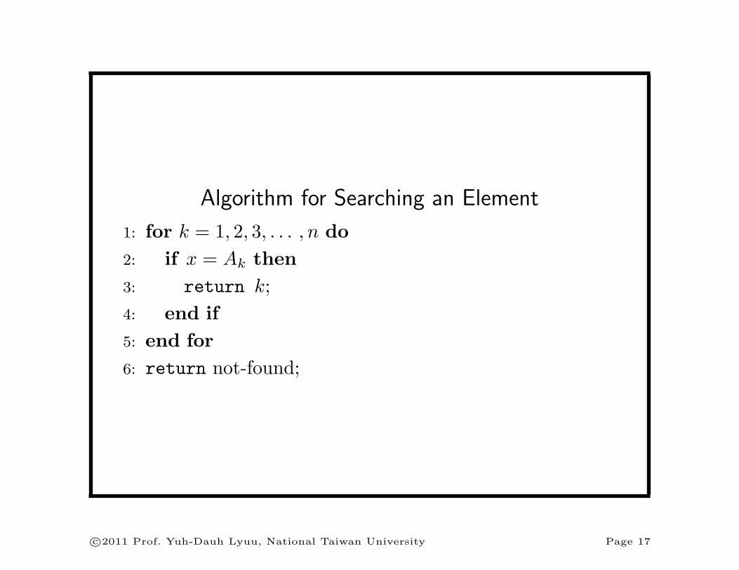
Algorithm for Searching an Element

1: for k = 1, 2, 3, . . . , n do2: if x = Ak then3: return k;4: end if5: end for6: return not-found;


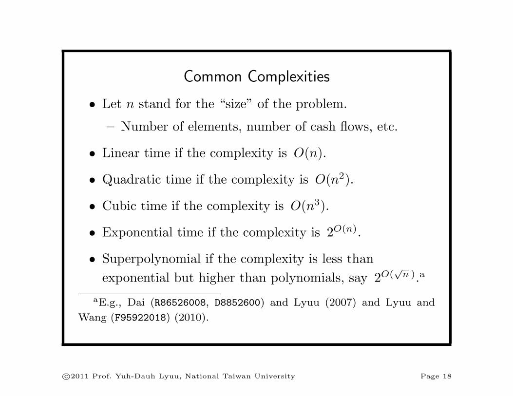
Common Complexities

• Let n stand for the “size” of the problem.

– Number of elements, number of cash flows, etc.

• Linear time if the complexity is O(n).

• Quadratic time if the complexity is O(n2).

• Cubic time if the complexity is O(n3).

• Exponential time if the complexity is 2O(n).

• Superpolynomial if the complexity is less thanexponential but higher than polynomials, say 2O(

√n ).a

aE.g., Dai (R86526008, D8852600) and Lyuu (2007) and Lyuu and

Wang (F95922018) (2010).


Basic Financial Mathematics


In the fifteenth centurymathematics was mainly concerned withquestions of commercial arithmetic and

the problems of the architect.— Joseph Alois Schumpeter (1883–1950)

I’m more concerned aboutthe return of my money than

the return on my money.— Will Rogers (1879–1935)


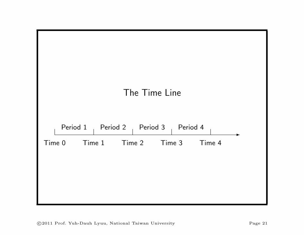
The Time Line

-Time 0 Time 1 Time 2 Time 3 Time 4

Period 1 Period 2 Period 3 Period 4


Time Value of Moneya

FV = PV(1 + r)n,

PV = FV× (1 + r)−n.

• FV (future value).

• PV (present value).

• r: interest rate.aFibonacci (1170–1240) and Irving Fisher (1867–1947).


Periodic Compounding

• Suppose the annual interest rate r is compounded m

times per annum.

• Then

1 →(1 +

r

m

)→

(1 +

r

m

)2

→(1 +

r

m

)3

→ · · ·

• Hence, after n years,

FV = PV(1 +

r

m

)nm

. (1)


Common Compounding Methods

• Annual compounding: m = 1.

• Semiannual compounding: m = 2.

• Quarterly compounding: m = 4.

• Monthly compounding: m = 12.

• Weekly compounding: m = 52.

• Daily compounding: m = 365.


Easy Translations

• An annual interest rate of r compounded m times ayear is “equivalent to” an interest rate of r/m per 1/m

year.

• If a loan asks for a return of 1% per month, the annualinterest rate will be 12% with monthly compounding.


Example

• Annual interest rate is 10% compounded twice perannum.

• Each dollar will grow to be

[ 1 + (0.1/2) ]2 = 1.1025

one year from now.

• The rate is equivalent to an interest rate of 10.25%compounded once per annum,

1 + 0.1025 = 1.1025


Continuous Compoundinga

• Let m →∞ so that(1 +

r

m

)m

→ er

in Eq. (1) on p. 23.

• ThenFV = PV× ern,

where e = 2.71828 . . . .aJacob Bernoulli (1654–1705) in 1685.


Continuous Compounding (concluded)

• Continuous compounding is easier to work with.

• Suppose the annual interest rate is r1 for n1 years andr2 for the following n2 years.

• Then the FV of one dollar will be

er1n1+r2n2 .


Efficient Algorithms for PV and FV

• The PV of the cash flow C1, C2, . . . , Cn at times1, 2, . . . , n is

C1

1 + y+

C2

(1 + y)2+ · · ·+ Cn

(1 + y)n.

• This formula and its variations are the engine behindmost of financial calculations.a

– What is y?

– What are Ci?

– What is n?a“Asset pricing theory all stems from one simple concept [...]: price

equals expected discounted payoff” (see Cochrane (2005)).


An Algorithm for Evaluating PV

1: x := 0;2: for i = 1, 2, . . . , n do3: x := x + Ci × /(1 + y)i;4: end for5: return x;

• The algorithm takes time proportional to∑ni=1 i = O(n2).

• Can improve it to O(n) if you apply ab = eb ln a.a

aThat is why we counted xy as taking one unit of time.


Another Algorithm for Evaluating PV

1: x := 0;2: d := 1 + y;3: for i = n, n− 1, . . . , 1 do4: x := (x + Ci)/d;5: end for6: return x;


Horner’s Rule: The Idea Behind p. 31

• This idea is(· · ·

((Cn

1 + y+ Cn−1

)1

1 + y+ Cn−2

)1

1 + y+ · · ·

)1

1 + y.

– Due to Horner (1786–1837) in 1819.

• The algorithm takes O(n) time.

• It is the most efficient possible in terms of the absolutenumber of arithmetic operations.a

aBorodin and Munro (1975).


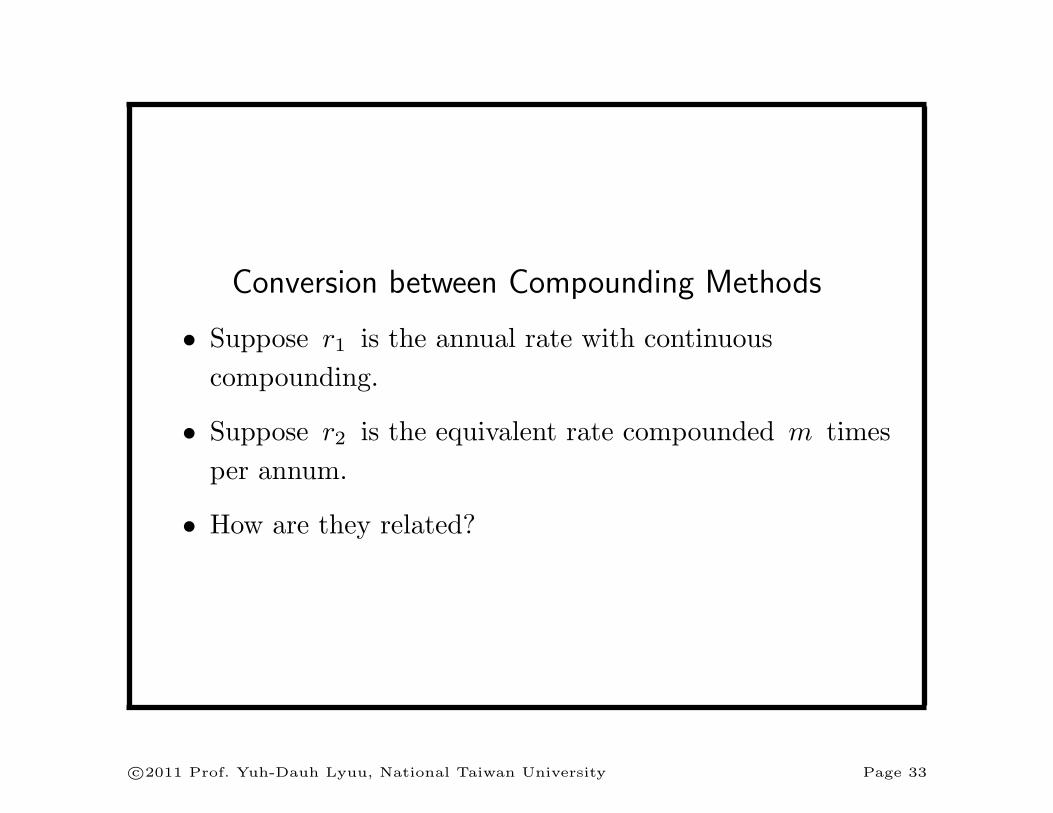
Conversion between Compounding Methods

• Suppose r1 is the annual rate with continuouscompounding.

• Suppose r2 is the equivalent rate compounded m timesper annum.

• How are they related?


Conversion between Compounding Methods(concluded)

• Both interest rates must produce the same amount ofmoney after one year.

• That is, (1 +

r2

m

)m

= er1 .

• Therefore,

r1 = m ln(1 +

r2

m

),

r2 = m(er1/m − 1

).


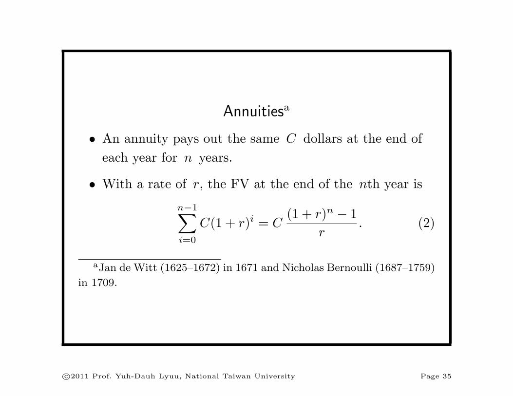
Annuitiesa

• An annuity pays out the same C dollars at the end ofeach year for n years.

• With a rate of r, the FV at the end of the nth year is

n−1∑

i=0

C(1 + r)i = C(1 + r)n − 1

r. (2)

aJan de Witt (1625–1672) in 1671 and Nicholas Bernoulli (1687–1759)

in 1709.


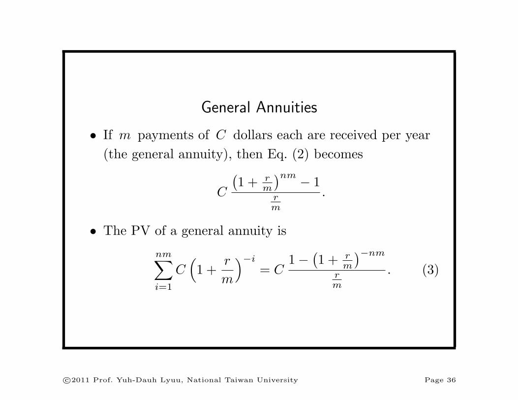
General Annuities

• If m payments of C dollars each are received per year(the general annuity), then Eq. (2) becomes

C

(1 + r

m

)nm − 1rm

.

• The PV of a general annuity is

nm∑

i=1

C(1 +

r

m

)−i

= C1− (

1 + rm

)−nm

rm

. (3)


Amortization

• It is a method of repaying a loan through regularpayments of interest and principal.

• The size of the loan (the original balance) is reduced bythe principal part of each payment.

• The interest part of each payment pays the interestincurred on the remaining principal balance.

• As the principal gets paid down over the term of theloan, the interest part of the payment diminishes.


Example: Home Mortgage

• By paying down the principal consistently, the risk tothe lender is lowered.

• When the borrower sells the house, the remainingprincipal is due the lender.

• Consider the equal-payment case, i.e., fixed-rate,level-payment, fully amortized mortgages.

– They are called traditional mortgages in the U.S.


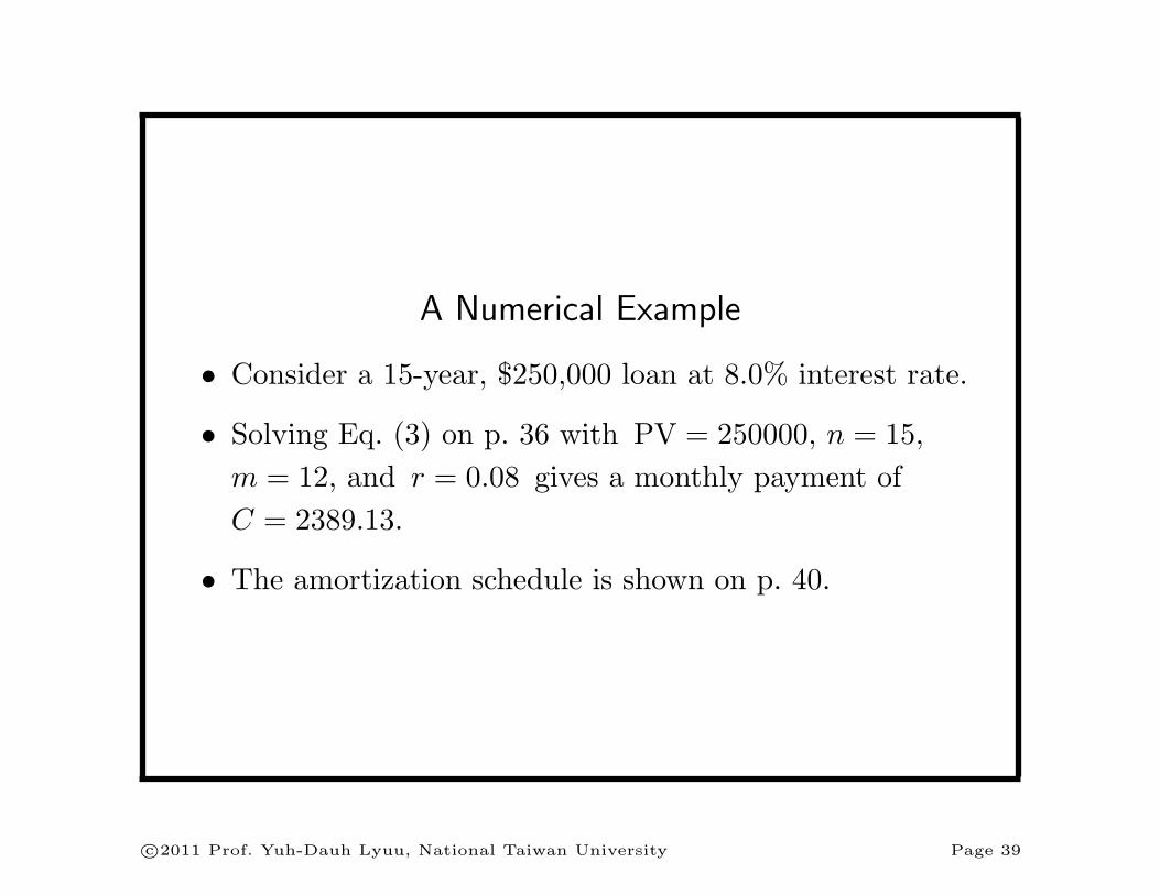
A Numerical Example

• Consider a 15-year, $250,000 loan at 8.0% interest rate.

• Solving Eq. (3) on p. 36 with PV = 250000, n = 15,m = 12, and r = 0.08 gives a monthly payment ofC = 2389.13.

• The amortization schedule is shown on p. 40.


Month Payment Interest PrincipalRemainingprincipal

250,000.000

1 2,389.13 1,666.667 722.464 249,277.536

2 2,389.13 1,661.850 727.280 248,550.256

3 2,389.13 1,657.002 732.129 247,818.128

· · ·178 2,389.13 47.153 2,341.980 4,730.899

179 2,389.13 31.539 2,357.591 2,373.308

180 2,389.13 15.822 2,373.308 0.000

Total 430,043.438 180,043.438 250,000.000


A Numerical Example (concluded)

In every month:

• The principal and interest parts add up to $2,389.13.

• The remaining principal is reduced by the amountindicated under the Principal heading.a

• The interest is computed by multiplying the remainingbalance of the previous month by 0.08/12.

aThis column varies with r. Thanks to a lively class discussion on

Feb 24, 2010.


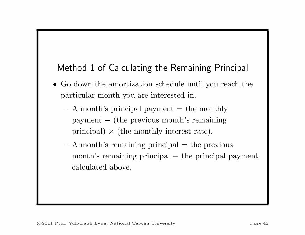
Method 1 of Calculating the Remaining Principal

• Go down the amortization schedule until you reach theparticular month you are interested in.

– A month’s principal payment = the monthlypayment − (the previous month’s remainingprincipal) × (the monthly interest rate).

– A month’s remaining principal = the previousmonth’s remaining principal − the principal paymentcalculated above.


Method 1 of Calculating the Remaining Principal(concluded)

• This method is relatively slow but is universal in itsapplicability.

• It can, for example, accommodate prepayment andvariable interest rates.


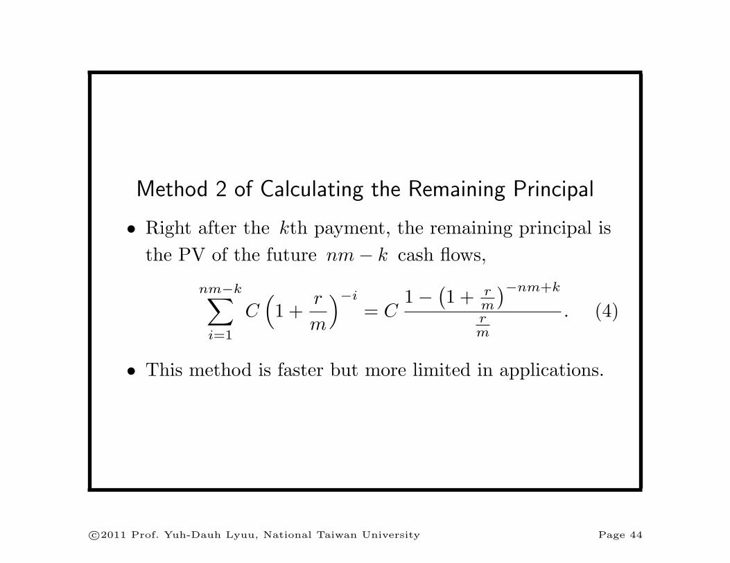
Method 2 of Calculating the Remaining Principal

• Right after the kth payment, the remaining principal isthe PV of the future nm− k cash flows,

nm−k∑

i=1

C(1 +

r

m

)−i

= C1− (

1 + rm

)−nm+k

rm

. (4)

• This method is faster but more limited in applications.


Yields

• The term yield denotes the return of investment.

• Two widely used yields are the bond equivalent yield(BEY) and the mortgage equivalent yield (MEY).

• Recall Eq. (1) on p. 23: FV = PV(1 + r

m

)nm.

• BEY corresponds to the r above that equates PV withFV when m = 2.

• MEY corresponds to the r above that equates PV withFV when m = 12.


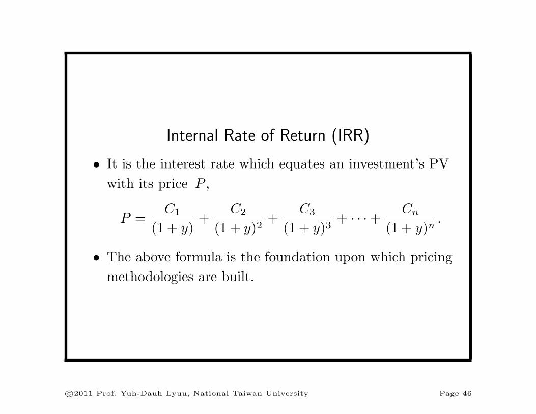
Internal Rate of Return (IRR)

• It is the interest rate which equates an investment’s PVwith its price P ,

P =C1

(1 + y)+

C2

(1 + y)2+

C3

(1 + y)3+ · · ·+ Cn

(1 + y)n.

• The above formula is the foundation upon which pricingmethodologies are built.


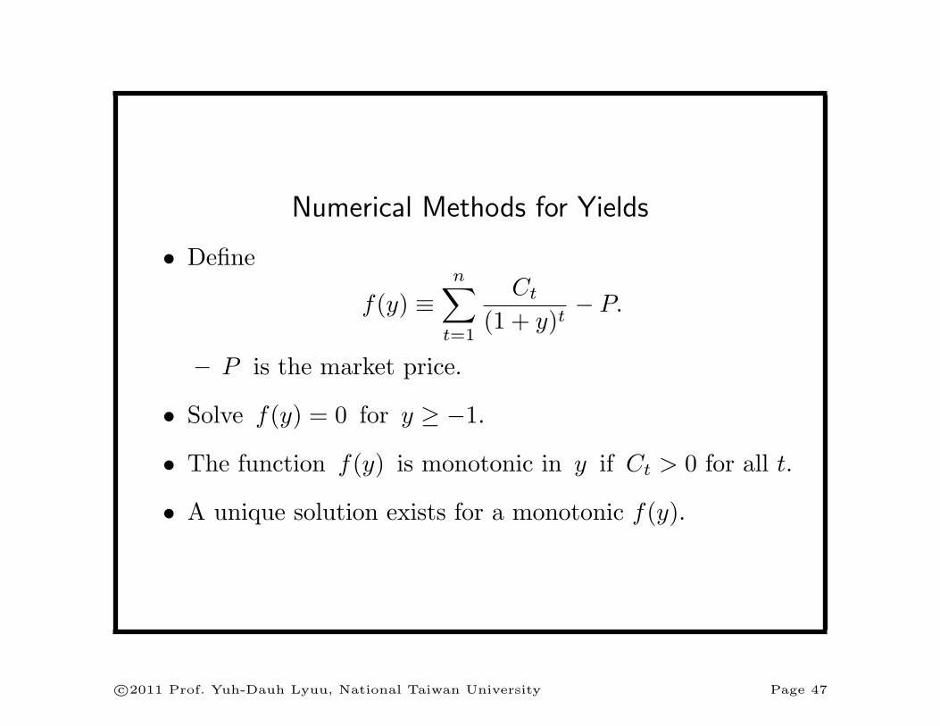
Numerical Methods for Yields

• Define

f(y) ≡n∑

t=1

Ct

(1 + y)t− P.

– P is the market price.

• Solve f(y) = 0 for y ≥ −1.

• The function f(y) is monotonic in y if Ct > 0 for all t.

• A unique solution exists for a monotonic f(y).


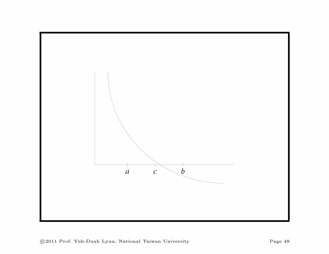
The Bisection Method

• Start with a and b where a < b and f(a) f(b) < 0.

• Then f(ξ) must be zero for some ξ ∈ [ a, b ].

• If we evaluate f at the midpoint c ≡ (a + b)/2, either(1) f(c) = 0, (2) f(a) f(c) < 0, or (3) f(c) f(b) < 0.

• In the first case we are done, in the second case wecontinue the process with the new bracket [ a, c ], and inthe third case we continue with [ c, b ].

• The bracket is halved in the latter two cases.

• After n steps, we will have confined ξ within a bracketof length (b− a)/2n.


D EF


The Newton-Raphson Method

• Converges faster than the bisection method.

• Start with a first approximation x0 to a root off(x) = 0.

• Then

xk+1 ≡ xk − f(xk)f ′(xk)

.

• When computing yields,

f ′(x) = −n∑

t=1

tCt

(1 + x)t+1.


xk xk 1

x

y

f x( )


The Secant Method

• A variant of the Newton-Raphson method.

• Replace differentiation with difference.

• Start with two approximations x0 and x1.

• Then compute the (k + 1)st approximation with

xk+1 = xk − f(xk)(xk − xk−1)f(xk)− f(xk−1)

.


The Secant Method (concluded)

• Its convergence rate is 1.618.

• This is slightly worse than the Newton-Raphsonmethod’s 2.

• But the secant method does not need to evaluate f ′(xk)needed by the Newton-Raphson method.

• This saves about 50% in computation efforts periteration.

• The convergence rate of the bisection method is 1.


Solving Systems of Nonlinear Equations

• It is not easy to extend the bisection method to higherdimensions.

• But the Newton-Raphson method can be extended tohigher dimensions.

• Let (xk, yk) be the kth approximation to the solution ofthe two simultaneous equations,

f(x, y) = 0,

g(x, y) = 0.


Solving Systems of Nonlinear Equations (concluded)

• The (k + 1)st approximation (xk+1, yk+1) satisfies thefollowing linear equations,

∂f(xk,yk)∂x

∂f(xk,yk)∂y

∂g(xk,yk)∂x

∂g(xk,yk)∂y

∆xk+1

∆yk+1

= −

f(xk, yk)

g(xk, yk)

,

where unknowns ∆xk+1 ≡ xk+1 − xk and∆yk+1 ≡ yk+1 − yk.

• The above has a unique solution for (∆xk+1, ∆yk+1)when the 2× 2 matrix is invertible.

• Set (xk+1, yk+1) = (xk + ∆xk+1, yk + ∆yk+1).


Zero-Coupon Bonds (Pure Discount Bonds)

• The price of a zero-coupon bond that pays F dollars inn periods is

F/(1 + r)n,

where r is the interest rate per period.

• Can meet future obligations without reinvestment risk.


Example

• The interest rate is 8% compounded semiannually.

• A zero-coupon bond that pays the par value 20 yearsfrom now will be priced at 1/(1.04)40, or 20.83%, of itspar value.

• It will be quoted as 20.83.

• If the bond matures in 10 years instead of 20, its pricewould be 45.64.


Level-Coupon Bonds

• Coupon rate.

• Par value, paid at maturity.

• F denotes the par value, and C denotes the coupon.

• Cash flow:

-6 6 66

1 2 3 n

C C C · · ·C + F

• Coupon bonds can be thought of as a matching packageof zero-coupon bonds, at least theoretically.a

a“You see, Daddy didn’t bake the cake, and Daddy isn’t the one who

gets to eat it. But he gets to slice the cake and hand it out. And when

he does, little golden crumbs fall off the cake. And Daddy gets to eat

those,” wrote Tom Wolfe (1931–) in Bonfire of the Vanities (1987).


Pricing Formula

P =

n∑i=1

C(1 + r

m

)i+

F(1 + r

m

)n

= C1− (

1 + rm

)−n

rm

+F(

1 + rm

)n . (5)

• n: number of cash flows.

• m: number of payments per year.

• r: annual rate compounded m times per annum.

• C = Fc/m when c is the annual coupon rate.

• Price P can be computed in O(1) time.


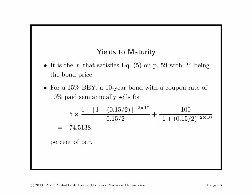
Yields to Maturity

• It is the r that satisfies Eq. (5) on p. 59 with P beingthe bond price.

• For a 15% BEY, a 10-year bond with a coupon rate of10% paid semiannually sells for

5× 1− [ 1 + (0.15/2) ]−2×10

0.15/2+

100[ 1 + (0.15/2) ]2×10

= 74.5138

percent of par.


Price Behavior (1)

• Bond prices fall when interest rates rise, and vice versa.

• “Only 24 percent answered the question correctly.”a

aCNN, December 21, 2001.


Price Behavior (2)

• A level-coupon bond sells

– at a premium (above its par value) when its couponrate is above the market interest rate;

– at par (at its par value) when its coupon rate is equalto the market interest rate;

– at a discount (below its par value) when its couponrate is below the market interest rate.


9% Coupon Bond

Yield (%)Price

(% of par)

7.5 113.37

8.0 108.65

8.5 104.19

9.0 100.00

9.5 96.04

10.0 92.31

10.5 88.79


Terminology

• Bonds selling at par are called par bonds.

• Bonds selling at a premium are called premium bonds.

• Bonds selling at a discount are called discount bonds.


Price Behavior (3): Convexity

0 0.05 0.1 0.15 0.2

Yield

0

250

500

750

1000

1250

1500

1750

Price


Day Count Conventions: Actual/Actual

• The first “actual” refers to the actual number of days ina month.

• The second refers to the actual number of days in acoupon period.

• The number of days between June 17, 1992, andOctober 1, 1992, is 106.

– 13 days in June, 31 days in July, 31 days in August,30 days in September, and 1 day in October.


Day Count Conventions: 30/360

• Each month has 30 days and each year 360 days.

• The number of days between June 17, 1992, andOctober 1, 1992, is 104.

– 13 days in June, 30 days in July, 30 days in August,30 days in September, and 1 day in October.

• In general, the number of days from dateD1 ≡ (y1,m1, d1) to date D2 ≡ (y2,m2, d2) is

360× (y2 − y1) + 30× (m2 −m1) + (d2 − d1).

• Complications: 31, Feb 28, and Feb 29.


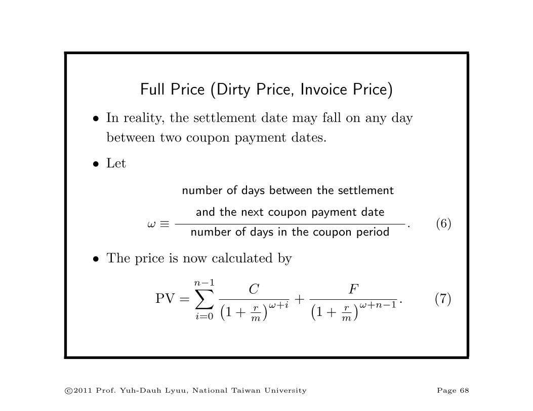
Full Price (Dirty Price, Invoice Price)

• In reality, the settlement date may fall on any daybetween two coupon payment dates.

• Let

ω ≡

number of days between the settlement

and the next coupon payment date

number of days in the coupon period. (6)

• The price is now calculated by

PV =n−1∑

i=0

C(1 + r

m

)ω+i+

F(1 + r

m

)ω+n−1 . (7)


Accrued Interest

• The buyer pays the invoice price (the quoted price plusthe accrued interest):

C ×

number of days from the last

coupon payment to the settlement date

number of days in the coupon period= C × (1− ω).

• The yield to maturity is the r satisfying Eq. (7) whenP is the invoice price.

• The quoted price in the U.S./U.K. does not include theaccrued interest; it is called the clean price or flat price.


-

6

coupon payment date

C(1− ω)

coupon payment date

¾ -(1− ω)% ¾ -ω%


Example (“30/360”)

• A bond with a 10% coupon rate and paying interestsemiannually, with clean price 111.2891.

• The maturity date is March 1, 1995, and the settlementdate is July 1, 1993.

• There are 60 days between July 1, 1993, and the nextcoupon date, September 1, 1993.


Example (“30/360”) (concluded)

• The accrued interest is (10/2)× 180−60180 = 3.3333 per

$100 of par value.

• The yield to maturity is 3%.

• This can be verified by Eq. (7) on p. 68 with

– ω = 60/180,

– m = 2,

– C = 5,

– PV= 111.2891 + 3.3333,

– r = 0.03.


Price Behavior (2) Revisited

• Before: A bond selling at par if the yield to maturityequals the coupon rate.

• But it assumed that the settlement date is on a couponpayment date.

• Now suppose the settlement date for a bond selling atpar (i.e., the quoted price is equal to the par value) fallsbetween two coupon payment dates.

• Then its yield to maturity is less than the coupon rate.

– The short reason: Exponential growth is replaced bylinear growth, hence “overpaying” the coupon.


principles of financial computing

Documents