principles of accounting review - dallas baptist...

Reading 2: Managerial Accounting Decision Making & Principles of Accounting Review (File 005r reference only)

1

Managerial Accounting Decision Making and Principles of Accounting Review

Managerial Accounting and Financial Accounting are quite different disciplines. Financial Accounting is primarily concerned with financial statements such as Balance Sheet, Income Statement and Cash Flows and the entries to bring about a correct display of those statements. Managerial Accounting, on the other hand, is concerned about how to use the numbers in making business decisions. Since this course is a decision making course, we will find our focus on reviewing decisions which are made using Managerial Accounting approaches. This review will presuppose you have taken a Managerial Accounting course and will develop decisions based on the belief you have this basic understanding. We will also review some Financial Accounting issues. In Managerial Accounting, the decision maker dwells on relevant information when making a decision. It is probably best if we look at a number of decision making problems. We will focus on marketing decisions and production decisions based on the use of relevant information. Relevant information depends on the decision under consideration. From the viewpoint of the Managerial Accountant relevant information is the predicted future costs and revenues that will differ among alternative courses of action. Wow, you say. That’s confusing. Okay, I say, let’s break it down into understandable key words. First, the definition refers to either cost or revenues. Managerial accountant decisions are always associated with either cost reductions or revenue enhancements. Second, predicted future is a term that means we are looking at something in the future and that something (cost or revenues) is estimated or predicted or forecasted. This means we are not looking at past costs and are only concerned with future costs. Historical costs have no bearing on the decisions we are going to make in the future. Remember we are looking at decisions from the viewpoint of a Managerial Accountant not a Financial Accountant. Financial Accountants are very interested in historical costs, but not the Managerial Accountant. Third, the phrase among alternatives means we have more than one choice. If there was only one choice there is nothing to evaluate thus only one decision is possible.


2

The idea can be summarized into two primary criteria. First, there must be expected future costs or revenues. Second, there must be a difference among alternatives. Several over simplified examples may serve to illustrate the point. #1) If a department manager’s salary is the same regardless of the number of products stocked, the salary is irrelevant to the selection and stocking of those products. #2) If gasoline costs $1.75 per gallon at one station and $1.80 at another station, there are two alternatives with difference between the alternatives so the cost is relevant to any decision we make. The historical cost of the gas last week is unimportant to our decision to purchase gas today (for the future). #3) Two oil changing station charge $19.95 to change the oil. These can be considered to be future costs, but they do not meet the criteria of having different alternatives. Any decision will not be made base on the future cost since there is really only one alternative to consider - $19.95. #4) Changing from copper to aluminum material for making ashtrays has the following information – Direct Labor Costs is $0.70 for either, but material costs change from $0.20 to $0.30 per ashtray. The material cost difference ($0.10) is relevant in making the decision, but the direct labor cost of $0.70 is not relevant in the decision to change from copper to aluminum. #5) Quantitative decisions are measured more easily than qualitative decisions. Quantitative decisions often lead to better decisions than qualitative ones. Qualitative decisions are difficult to measure. A union causes a manager to not purchase and install robotic equipment that would eliminate union jobs, although the decision is financially a good one for the company. Merc has found a drug for curing a deadly disease, but the market is small and unprofitable. Merc chooses to market the drug because of the life saving nature of the drug. Before we work thorough examples of everyday decisions, let’s take a time out and review some of the basics of Financial Accounting. The Managerial Accountant will use data developed and gathered by the Financial Accountant when making decisions. Financial Accountants prepare three primary financial statements. First is the Income Statement which is a statement of the profit and loss of the operation. It is for a period of time usually ending at the end of the fiscal year which might be the calendar year. Second is the Balance Sheet which is a statement of the Assets and Liabilities of an operation at a particular point in time, usually the end of the year. When the business closes at the end of the fiscal or calendar


3

year, the Income Statement is reset to zero and begins measuring profitability all over again. Let’s assume the year end is 12-31-XX for a company. At 12-31-X1, there would be a Balance Sheet and an Income Statement. Assuming there was a profit, the profit is at the bottom of the Income Statement, but it would also be reflected in the Equity section of the Balance Sheet as an account called Retained Earnings. Usually there are two retained earnings accounts, one for prior periods and one for the current period. Retained earning is the net account that ties the Income Statement and the Balance Sheet together. In other words, everything in the Income Statement will be rolled into the Balance Sheet as a single entry at the end of the fiscal year. The Income Statement to begins at zero for all entries at 1-01-X2 (or the start of a new fiscal year). The only other major statement of interest to the Financial Accountant is the Cash Flow Statement. In the Balance Sheet there is an account called “Cash”. There are two methods of accounting – cash accounting where all transactions are recorded based on when you receive the money and when you write the checks and accrual accounting where you match the income and expenses to the period of interest. For example, you may pay $15,000 for a three year insurance policy. This is a cash payment of $15,000, but for purposes of the Income Statement an expense of $5,000 would be recorded for the year. The $10,000 balance would be deferred and recorded equally in the next two fiscal year Income Statements. The cash & cash equivalents account(s) (Balance Sheet accounts) have been recorded based on cash-in, cash-out. The Cash Flow Statement converts this cash basis account to an accrual basis account, thus matching periods of expense and income. This is probably one of the more important statements and one of the more difficult to prepare. Businesses tend to go broke from the lack of cash not the lack of income. The Financial Accountant is interested in the proper development and recordation of transactions for these three statements using generally accepted accounting principles (GAAP). The Managerial Accountant will take the information developed by the Financial Accountant and use it to make business decisions. The Managerial Accountant is not bound by the same GAAP principles as the Financial Accountant, since business decisions consider tactical as well as strategic planning rather than accurate recordation of historical data. The Managerial Accountant will use the information developed by the Financial Accountant as a starting point in making day to day business decisions. Statement Examples: Below are examples of all three statements beginning with a comparative Balance Sheet, Income Statement and a Cash Flow Statement.


4

Davis Corporation Comparative Balance Sheets

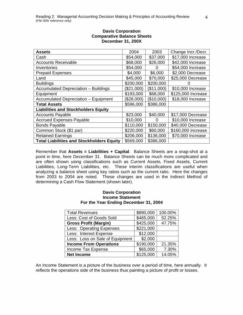
December 31, 200X Assets 2004 2003 Change Incr./Decr.Cash $54,000 $37,000 $17,000 Increase Accounts Receivable $68,000 $26,000 $42,000 Increase Inventories $54,000 0 $54,000 Increase Prepaid Expenses $4,000 $6,000 $2,000 Decrease Land $45,000 $70,000 $25,000 Decrease Buildings $200,000 $200,000 0 Accumulated Depreciation – Buildings ($21,000) ($11,000) $10,000 Increase Equipment $193,000 $68,000 $125,000 IncreaseAccumulated Depreciation – Equipment ($28,000) ($10,000) $18,000 Increase Total Assets $596,000 $386,000 Liabilities and Stockholders Equity Accounts Payable $23,000 $40,000 $17,000 Decrease Accrued Expenses Payable $10,000 0 $10,000 Increase Bonds Payable $110,000 $150,000 $40,000 Decrease Common Stock ($1 par) $220,000 $60,000 $160,000 IncreaseRetained Earnings $206,000 $136,000 $70,000 Increase Total Liabilities and Stockholders Equity $569,000 $386,000 Remember that Assets = Liabilities + Capital. Balance Sheets are a snap-shot at a point in time, here December 31. Balance Sheets can be much more complicated and are often shown using classifications such as Current Assets, Fixed Assets, Current Liabilities, Long-Term Liabilities, etc. These interim classifications are useful when analyzing a balance sheet using key ratios such as the current ratio. Here the changes from 2003 to 2004 are noted. These changes are used in the Indirect Method of determining a Cash Flow Statement (shown later).

Davis Corporation Income Statement

For the Year Ending December 31, 2004

Total Revenues $890,000 100.00% Less: Cost of Goods Sold $465,000 52.25% Gross Profit (Margin) $425,000 47.75% Less: Operating Expenses $221,000 Less: Interest Expense $12,000 Less: Loss on Sale of Equipment $2,000 Income From Operations $190,000 21.35% Income Tax Expense $65,000 7.30% Net Income $125,000 14.05%

An Income Statement is a picture of the business over a period of time, here annually. It reflects the operations side of the business thus painting a picture of profit or losses.


5

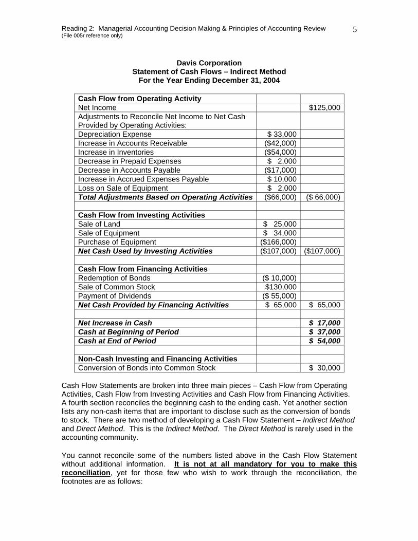
Davis Corporation

Statement of Cash Flows – Indirect Method For the Year Ending December 31, 2004

Cash Flow from Operating Activity Net Income $125,000Adjustments to Reconcile Net Income to Net Cash Provided by Operating Activities:

Depreciation Expense $ 33,000 Increase in Accounts Receivable ($42,000) Increase in Inventories ($54,000) Decrease in Prepaid Expenses $ 2,000 Decrease in Accounts Payable ($17,000) Increase in Accrued Expenses Payable $ 10,000 Loss on Sale of Equipment $ 2,000 Total Adjustments Based on Operating Activities ($66,000) ($ 66,000) Cash Flow from Investing Activities Sale of Land $ 25,000 Sale of Equipment $ 34,000 Purchase of Equipment ($166,000) Net Cash Used by Investing Activities ($107,000) ($107,000) Cash Flow from Financing Activities Redemption of Bonds ($ 10,000) Sale of Common Stock $130,000 Payment of Dividends ($ 55,000) Net Cash Provided by Financing Activities $ 65,000 $ 65,000 Net Increase in Cash $ 17,000Cash at Beginning of Period $ 37,000Cash at End of Period $ 54,000 Non-Cash Investing and Financing Activities Conversion of Bonds into Common Stock $ 30,000

Cash Flow Statements are broken into three main pieces – Cash Flow from Operating Activities, Cash Flow from Investing Activities and Cash Flow from Financing Activities. A fourth section reconciles the beginning cash to the ending cash. Yet another section lists any non-cash items that are important to disclose such as the conversion of bonds to stock. There are two method of developing a Cash Flow Statement – Indirect Method and Direct Method. This is the Indirect Method. The Direct Method is rarely used in the accounting community. You cannot reconcile some of the numbers listed above in the Cash Flow Statement without additional information. It is not at all mandatory for you to make this reconciliation, yet for those few who wish to work through the reconciliation, the footnotes are as follows:


6

1. Operating Expenses include depreciation expense of $33,000 and charges from

prepaid expenses of $2,000. 2. Land was sold at its book value for cash. 3. Cash dividends of $55,000 were declared and paid in 2003. 4. Interest Expense of $12,000 was paid in cash. 5. Equipments with a cost of $166,000 was purchased for cash. Equipments with a

cost of $41,000 and a book value of $36,000 was sold for $34,000 cash. 6. Bonds of $10,000 were redeemed at their book value for cash. Bonds of

$30,000 were converted into common stock. 7. Common stock ($1 par) of $130,000 was issued for cash. 8. Accounts payable pertain to merchandise suppliers.

With these footnotes you should be able to, if you want to, create the Cash Flow Statement using the Balance Sheet and the Income Statement previously given. (Footnote reference only: Statements are File 006r) Let’s now look at some very specific relationships that bear heavily on decision making from the viewpoint of the Managerial Accountant. Cost-Volume-Profit Relationships There are two basic relationships associated with CVP relationships. The first is Cost Behavior Analysis and the second is Cost-Volume-Profit Analysis.

• Cost Behavior Analysis

Under this analysis we evaluate variable costs, fixed costs, relevant range and mixed costs.

• Cost-Volume-Profit Analysis

Under this analysis we evaluate contribution margin, break-even analysis, and target net income.

Let’s look at the details of each idea. Cost Behavior Analysis Variable costs are costs that vary in total directly and proportionately with changes in the activity level. If the level of activity increases 15%, total variable cost will increase 15%. If the level of activity decreases 10%, total variable cost decreases 10%. Direct material and direct labor are the best examples of variable cost. Variable costs also include such things as sales commissions, cost of goods sold, freight-out, gasoline for an airline or trucking company. One key to using variable cost is to remember that variable cost may be defined as cost that remains the same PER UNIT at every level of activity.


7

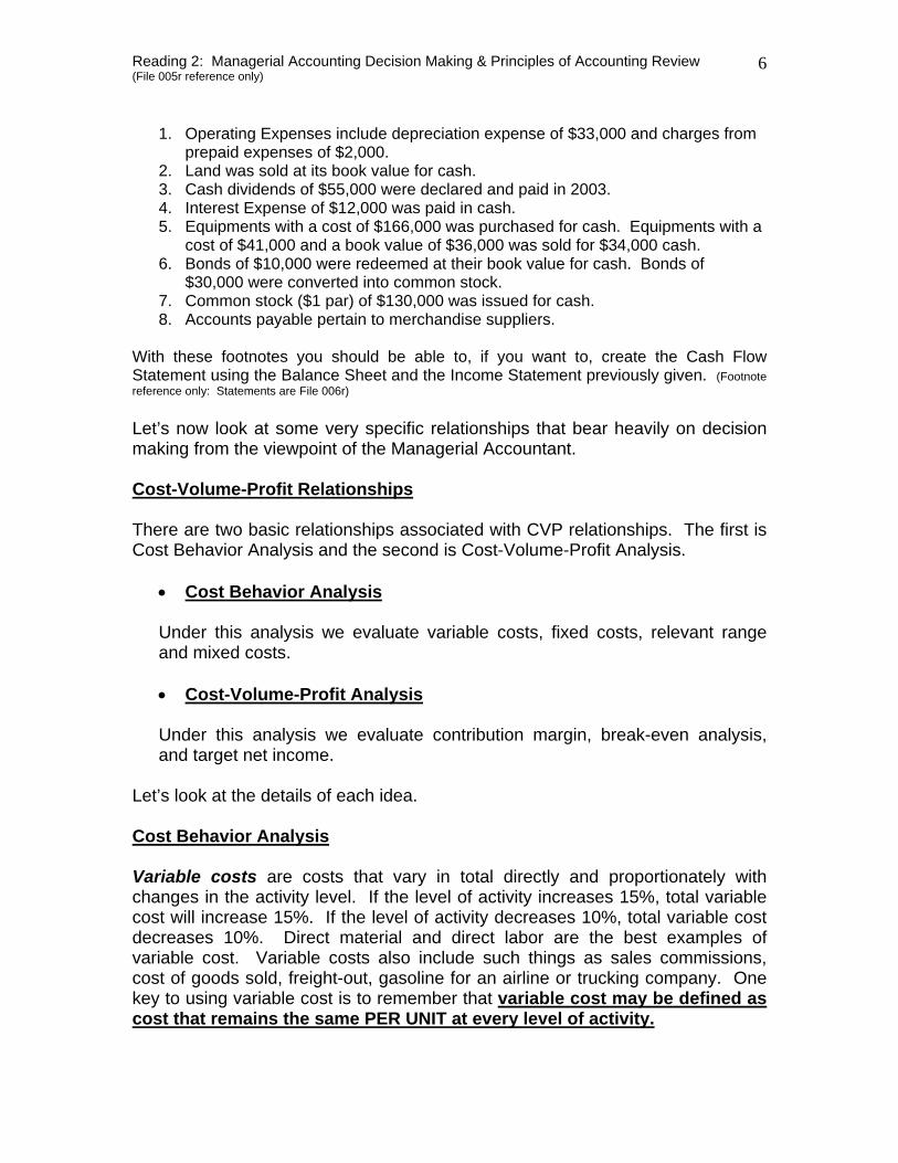
To illustrate, let’s suppose that the variable cost per unit to produce a widget is $20. At unit production of 1,000, the total cost is $20,000 ($20 per unit times 1,000 units). At unit production of 2,000, the total cost increases to $40,000 ($20 times 2,000). A graph can be used to visually reflect this relationship. Graph A: Total Variable Cost

Widgets - Total Variable Cost

0

20

40

60

80

100

120

1 2 3 4 5

Wi dge t s P r oduc e d ( 0 0 0 )

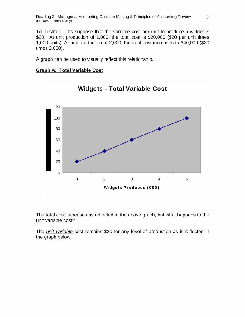
The total cost increases as reflected in the above graph, but what happens to the unit variable cost? The unit variable cost remains $20 for any level of production as is reflected in the graph below.


8

Graph B: Variable Cost Per Unit

Widgets - Variable Cost Per Unit

0

5

10

15

20

25

30

35

40

1 2 3 4 5

Widgets Produced (000)

Var

iabl

e Co

st P

er U

nit

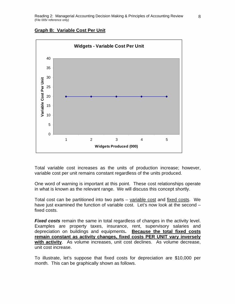
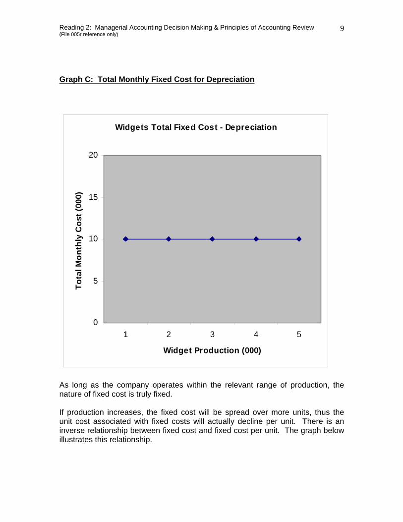
Total variable cost increases as the units of production increase; however, variable cost per unit remains constant regardless of the units produced. One word of warning is important at this point. These cost relationships operate in what is known as the relevant range. We will discuss this concept shortly. Total cost can be partitioned into two parts – variable cost and fixed costs. We have just examined the function of variable cost. Let’s now look at the second – fixed costs. Fixed costs remain the same in total regardless of changes in the activity level. Examples are property taxes, insurance, rent, supervisory salaries and depreciation on buildings and equipments. Because the total fixed costs remain constant as activity changes, fixed costs PER UNIT vary inversely with activity. As volume increases, unit cost declines. As volume decrease, unit cost increase. To illustrate, let’s suppose that fixed costs for depreciation are $10,000 per month. This can be graphically shown as follows.


9

Graph C: Total Monthly Fixed Cost for Depreciation

Widgets Total Fixed Cost - Depreciation

0

5

10

15

20

1 2 3 4 5

Widget Production (000)

Tota

l Mon

thly

Cos

t (00

0)

As long as the company operates within the relevant range of production, the nature of fixed cost is truly fixed. If production increases, the fixed cost will be spread over more units, thus the unit cost associated with fixed costs will actually decline per unit. There is an inverse relationship between fixed cost and fixed cost per unit. The graph below illustrates this relationship.


10

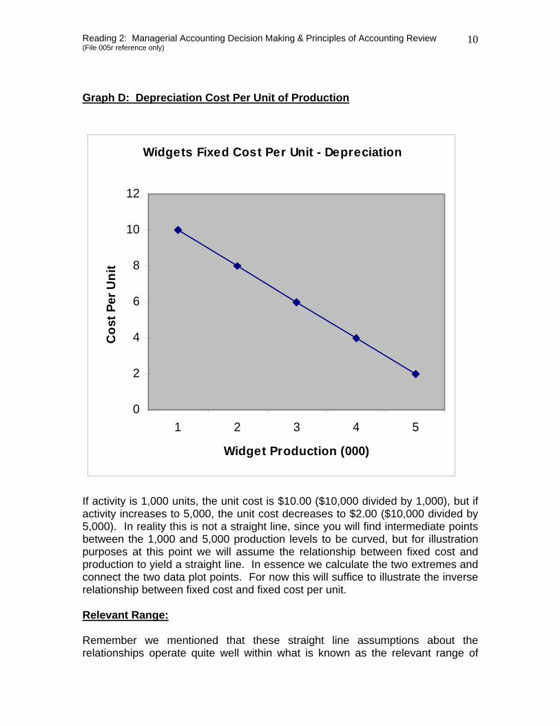
Graph D: Depreciation Cost Per Unit of Production

Widgets Fixed Cost Per Unit - Depreciation

0

2

4

6

8

10

12

1 2 3 4 5

Widget Production (000)

Cos

t Per

Uni

t

If activity is 1,000 units, the unit cost is $10.00 ($10,000 divided by 1,000), but if activity increases to 5,000, the unit cost decreases to $2.00 ($10,000 divided by 5,000). In reality this is not a straight line, since you will find intermediate points between the 1,000 and 5,000 production levels to be curved, but for illustration purposes at this point we will assume the relationship between fixed cost and production to yield a straight line. In essence we calculate the two extremes and connect the two data plot points. For now this will suffice to illustrate the inverse relationship between fixed cost and fixed cost per unit. Relevant Range: Remember we mentioned that these straight line assumptions about the relationships operate quite well within what is known as the relevant range of


11

production. Production can vary from zero (0) capacity to 100% capacity. Few companies produce on either of the two extreme ends of the entire range of production. In other words, few companies operate at zero or at 100% of capacity. At the extremes the functions of both fixed and variable cost do not take on a true linear character. Let’s look at some of the problems with those assumptions we have made about the straight line relationship for both fixed and variable cost. The relevant range is a concept that is often ignored by many decision makers, but should not be. Working with fixed and variable costs, the assumption is made they exhibit straight line relationships at all levels of production. This assumption is not reasonable. Many factors will change the costs at various levels of production. When discussing the relevant range, you must consider the entire range of production available to a company. A company can produce at 0% capacity or at 100% capacity, but neither is likely. Usually companies stay within a range of 40% to 80% of capacity. Often variable costs exhibit a curve-linear relationship when production is less than 40% or greater than 80%. For example, a company operating at the lower end of capacity will not be able to take advantage of quantity discounts, or may not be able to afford specialized labor. At the high levels of activity labor costs may increase because of overtime pay or excess spoilage caused by worker fatigue. These anomalies at the extreme ends (lower and upper) of the cost will cause variable cost to operate in something other than a linear fashion. Inside the relevant range; however, the variable cost tend to operate in a straight line fashion. Often fixed costs exhibit stair-stepped cost behavior. Some examples are new product development and management training programs. When the company is operating in the lower range of capacity the fixed cost will be less but move to the higher range and the cost will increase yet will still maintain a straight line relationship, but at a higher level of activity. As long as the company operates in the relevant range of capacity, the relationship can be considered to be a straight line relationship. Most companies will establish their budgeted cost based on some assumption of capacity. This assumption becomes the relevant range. Mixed Costs: Sometimes costs can include both fixed and variable costs. When this occurs they are known as mixed costs. A good example of mixed cost is a rental trailer or vehicle. You will pay $29.95 per day (fixed) plus $0.50 per mile (variable). As miles increase the total cost increases. For purposes of CVP analysis (explained below), mixed costs must be classified into their fixed and variable components. This can be a reasonably complex method. Usually a division will be made at the end of a time period rather than a case by case basis.


12

Review of fixed and variable costs, mixed costs and the relevant range is important as we look at cases. Another useful idea is cost-volume-profit analysis (CVP). Cost-Volume-Profit Analysis The idea behind Cost-Volume-Profit (CVP) analysis is the study of the effect of changes in costs and volume on a company’s profit. This concept is important in setting selling prices, determining product mix and maximizing use of the production facilities among other things. When using CVP interrelationships, the volume (level of activity), unit selling price, variable cost per unit, total fixed cost and the sales mix are all important factors to be considered. Notice we mentioned unit cost. Most decisions can be made without having to know the total cost, but unit cost becomes very important. In short, the Managerial Accountant does not need to complete a full blown balance sheet or income statement to make decisions. Often the idea of contribution margin in dollars or units can be useful. Contribution margin is an extremely important concept for the Managerial Accountant. Contribution margin is the amount of revenue remaining after deducting variable costs. For example, assume you own a VCR sales business with several locations. Your sales are 1,000 units with total revenues of $500,000. Variable costs are $300,000. The contribution margin is $200,000 ($500,000 - $300,000). You can also determine a contribution margin per unit. If your contribution margin is $200,000 and your sales are 1,000 units, the contribution margin per unit is $200 ($200,000 ÷ 1,000). If we, for the sake of illustration, assume the fixed costs are also $200,000, we can state that every unit sold will contribute $200 to cover the fixed costs. With 1,000 units additional units sold, we reach breakeven (1,000 units times $200 per unit = $200,000 contributed to cover fixed cost), thus any sale above the 1,000 units in sales volume will contribute $200 to income. If we sell an additional 1,500 units, the additional contribution margin will be $100,000 (1,500 units sold less 1,000 breakeven = 500 units times $200 contribution margin per unit). Total Revenues $500,000 Less: Variable Cost - 300,000 Equals: Contribution Margin * $200,000 Less: Fixed Cost (Assumption) $200,000 Breakeven Zero *To Generate $200,000 in Revenues to Cover the Fixed Cost The Company Must Sell 1,000 new units at a contribution margin per unit of $200. Selling anything over and above the 1,000 units will yield additional contribution margin. For example: 500 additional units times $200 = $100,000 additional revenues.


13

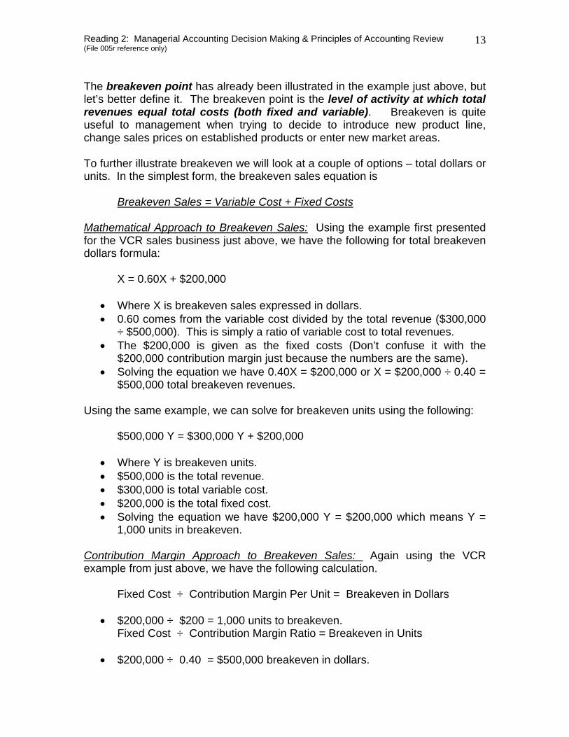
The breakeven point has already been illustrated in the example just above, but let’s better define it. The breakeven point is the level of activity at which total revenues equal total costs (both fixed and variable). Breakeven is quite useful to management when trying to decide to introduce new product line, change sales prices on established products or enter new market areas. To further illustrate breakeven we will look at a couple of options – total dollars or units. In the simplest form, the breakeven sales equation is Breakeven Sales = Variable Cost + Fixed Costs Mathematical Approach to Breakeven Sales: Using the example first presented for the VCR sales business just above, we have the following for total breakeven dollars formula: X = 0.60X + $200,000

• Where X is breakeven sales expressed in dollars. • 0.60 comes from the variable cost divided by the total revenue ($300,000

÷ $500,000). This is simply a ratio of variable cost to total revenues. • The $200,000 is given as the fixed costs (Don’t confuse it with the

$200,000 contribution margin just because the numbers are the same). • Solving the equation we have 0.40X = $200,000 or X = $200,000 ÷ 0.40 =

$500,000 total breakeven revenues. Using the same example, we can solve for breakeven units using the following: $500,000 Y = $300,000 Y + $200,000

• Where Y is breakeven units. • $500,000 is the total revenue. • $300,000 is total variable cost. • $200,000 is the total fixed cost. • Solving the equation we have $200,000 Y = $200,000 which means Y =

1,000 units in breakeven. Contribution Margin Approach to Breakeven Sales: Again using the VCR example from just above, we have the following calculation.

Fixed Cost ÷ Contribution Margin Per Unit = Breakeven in Dollars

• $200,000 ÷ $200 = 1,000 units to breakeven. Fixed Cost ÷ Contribution Margin Ratio = Breakeven in Units

• $200,000 ÷ 0.40 = $500,000 breakeven in dollars.


14

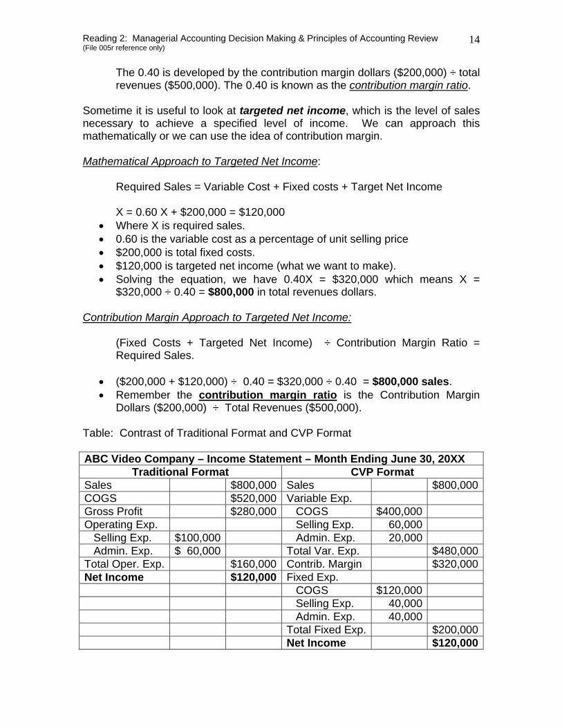
The 0.40 is developed by the contribution margin dollars ($200,000) ÷ total revenues ($500,000). The 0.40 is known as the contribution margin ratio.

Sometime it is useful to look at targeted net income, which is the level of sales necessary to achieve a specified level of income. We can approach this mathematically or we can use the idea of contribution margin. Mathematical Approach to Targeted Net Income: Required Sales = Variable Cost + Fixed costs + Target Net Income X = 0.60 X + $200,000 = $120,000

• Where X is required sales. • 0.60 is the variable cost as a percentage of unit selling price • $200,000 is total fixed costs. • $120,000 is targeted net income (what we want to make). • Solving the equation, we have 0.40X = $320,000 which means X =

$320,000 ÷ 0.40 = $800,000 in total revenues dollars. Contribution Margin Approach to Targeted Net Income: (Fixed Costs + Targeted Net Income) ÷ Contribution Margin Ratio = Required Sales.

• ($200,000 + $120,000) ÷ 0.40 = $320,000 ÷ 0.40 = $800,000 sales. • Remember the contribution margin ratio is the Contribution Margin

Dollars ($200,000) ÷ Total Revenues ($500,000). Table: Contrast of Traditional Format and CVP Format ABC Video Company – Income Statement – Month Ending June 30, 20XX

Traditional Format CVP Format Sales $800,000 Sales $800,000COGS $520,000 Variable Exp. Gross Profit $280,000 COGS $400,000 Operating Exp. Selling Exp. 60,000 Selling Exp. $100,000 Admin. Exp. 20,000 Admin. Exp. $ 60,000 Total Var. Exp. $480,000Total Oper. Exp. $160,000 Contrib. Margin $320,000Net Income $120,000 Fixed Exp. COGS $120,000 Selling Exp. 40,000 Admin. Exp. 40,000 Total Fixed Exp. $200,000 Net Income $120,000


15

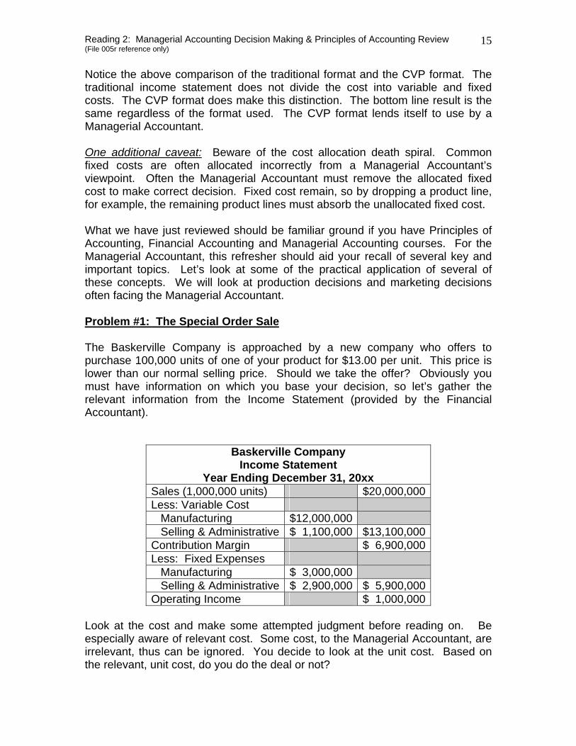
Notice the above comparison of the traditional format and the CVP format. The traditional income statement does not divide the cost into variable and fixed costs. The CVP format does make this distinction. The bottom line result is the same regardless of the format used. The CVP format lends itself to use by a Managerial Accountant. One additional caveat: Beware of the cost allocation death spiral. Common fixed costs are often allocated incorrectly from a Managerial Accountant’s viewpoint. Often the Managerial Accountant must remove the allocated fixed cost to make correct decision. Fixed cost remain, so by dropping a product line, for example, the remaining product lines must absorb the unallocated fixed cost. What we have just reviewed should be familiar ground if you have Principles of Accounting, Financial Accounting and Managerial Accounting courses. For the Managerial Accountant, this refresher should aid your recall of several key and important topics. Let’s look at some of the practical application of several of these concepts. We will look at production decisions and marketing decisions often facing the Managerial Accountant. Problem #1: The Special Order Sale The Baskerville Company is approached by a new company who offers to purchase 100,000 units of one of your product for $13.00 per unit. This price is lower than our normal selling price. Should we take the offer? Obviously you must have information on which you base your decision, so let’s gather the relevant information from the Income Statement (provided by the Financial Accountant).

Baskerville Company Income Statement

Year Ending December 31, 20xx Sales (1,000,000 units) $20,000,000 Less: Variable Cost Manufacturing $12,000,000 Selling & Administrative $ 1,100,000 $13,100,000 Contribution Margin $ 6,900,000 Less: Fixed Expenses Manufacturing $ 3,000,000 Selling & Administrative $ 2,900,000 $ 5,900,000 Operating Income $ 1,000,000

Look at the cost and make some attempted judgment before reading on. Be especially aware of relevant cost. Some cost, to the Managerial Accountant, are irrelevant, thus can be ignored. You decide to look at the unit cost. Based on the relevant, unit cost, do you do the deal or not?


16

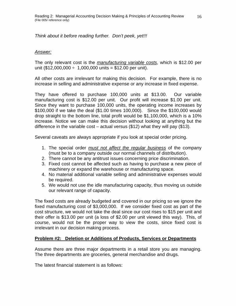
Think about it before reading further. Don’t peek, yet!!! Answer: The only relevant cost is the manufacturing variable costs, which is $12.00 per unit ($12,000,000 ÷ 1,000,000 units = $12.00 per unit). All other costs are irrelevant for making this decision. For example, there is no increase in selling and administrative expense or any increase in fixed expense. They have offered to purchase 100,000 units at $13.00. Our variable manufacturing cost is $12.00 per unit. Our profit will increase $1.00 per unit. Since they want to purchase 100,000 units, the operating income increases by $100,000 if we take the deal ($1.00 times 100,000). Since the $100,000 would drop straight to the bottom line, total profit would be $1,100,000, which is a 10% increase. Notice we can make this decision without looking at anything but the difference in the variable cost – actual versus ($12) what they will pay ($13). Several caveats are always appropriate if you look at special order pricing.

1. The special order must not affect the regular business of the company (must be to a company outside our normal channels of distribution).

2. There cannot be any antitrust issues concerning price discrimination. 3. Fixed cost cannot be affected such as having to purchase a new piece of

machinery or expand the warehouse or manufacturing space. 4. No material additional variable selling and administrative expenses would

be required. 5. We would not use the idle manufacturing capacity, thus moving us outside

our relevant range of capacity. The fixed costs are already budgeted and covered in our pricing so we ignore the fixed manufacturing cost of $3,000,000. If we consider fixed cost as part of the cost structure, we would not take the deal since our cost rises to $15 per unit and their offer is $13.00 per unit (a loss of $2.00 per unit viewed this way). This, of course, would not be the proper way to view the costs, since fixed cost is irrelevant in our decision making process. Problem #2: Deletion or Additions of Products, Services or Departments Assume there are three major departments in a retail store you are managing. The three departments are groceries, general merchandise and drugs. The latest financial statement is as follows:


17

Retail Store Income Statement

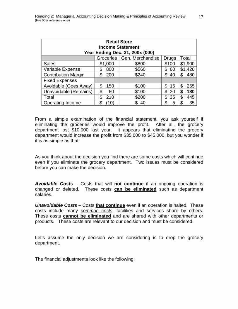
Year Ending Dec. 31, 200x (000) Groceries Gen. Merchandise Drugs Total Sales $1,000 $800 $100 $1,900Variable Expense $ 800 $560 $ 60 $1,420Contribution Margin $ 200 $240 $ 40 $ 480Fixed Expenses Avoidable (Goes Away) $ 150 $100 $ 15 $ 265Unavoidable (Remains) $ 60 $100 $ 20 $ 180Total $ 210 $200 $ 35 $ 445Operating Income $ (10) $ 40 $ 5 $ 35

From a simple examination of the financial statement, you ask yourself if eliminating the groceries would improve the profit. After all, the grocery department lost $10,000 last year. It appears that eliminating the grocery department would increase the profit from $35,000 to $45,000, but you wonder if it is as simple as that. As you think about the decision you find there are some costs which will continue even if you eliminate the grocery department. Two issues must be considered before you can make the decision. Avoidable Costs – Costs that will not continue if an ongoing operation is changed or deleted. These costs can be eliminated such as department salaries. Unavoidable Costs – Costs that continue even if an operation is halted. These costs include many common costs, facilities and services share by others. These costs cannot be eliminated and are shared with other departments or products. These costs are relevant to our decision and must be considered. Let’s assume the only decision we are considering is to drop the grocery department. The financial adjustments look like the following:


18

Decision Process (000)

Item Original Summary Fin.

Statement

Decision to Drop Grocery

After Dropping Grocery

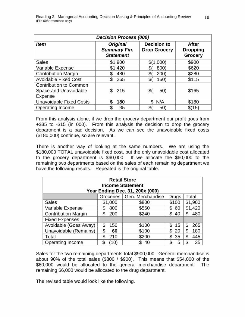
Sales $1,900 $(1,000) $900 Variable Expense $1,420 $( 800) $620 Contribution Margin $ 480 $( 200) $280 Avoidable Fixed Cost $ 265 $( 150) $115 Contribution to Common Space and Unavoidable Expense

$ 215

$( 50)

$165

Unavoidable Fixed Costs $ 180 $ N/A $180 Operating Income $ 35 $( 50) $(15) From this analysis alone, if we drop the grocery department our profit goes from +$35 to -$15 (in 000). From this analysis the decision to drop the grocery department is a bad decision. As we can see the unavoidable fixed costs ($180,000) continue, so are relevant. There is another way of looking at the same numbers. We are using the $180,000 TOTAL unavoidable fixed cost, but the only unavoidable cost allocated to the grocery department is $60,000. If we allocate the $60,000 to the remaining two departments based on the sales of each remaining department we have the following results. Repeated is the original table.

Retail Store Income Statement

Year Ending Dec. 31, 200x (000) Groceries Gen. Merchandise Drugs Total Sales $1,000 $800 $100 $1,900Variable Expense $ 800 $560 $ 60 $1,420Contribution Margin $ 200 $240 $ 40 $ 480Fixed Expenses Avoidable (Goes Away) $ 150 $100 $ 15 $ 265Unavoidable (Remains) $ 60 $100 $ 20 $ 180Total $ 210 $200 $ 35 $ 445Operating Income $ (10) $ 40 $ 5 $ 35

Sales for the two remaining departments total $900,000. General merchandise is about 90% of the total sales ($800 / $900). This means that $54,000 of the $60,000 would be allocated to the general merchandise department. The remaining $6,000 would be allocated to the drug department. The revised table would look like the following.


19

Retail Store

Income Statement Year Ending Dec. 31, 200x (000)

Groceries (Shown as

Reference Only-Not in Totals)

General Merchandise

Drugs Totals for Remaining Two

Departments

Sales $1,000 $800 $100 $900 Variable Expense $ 800 $560 $ 60 $620 Contribution Margin

$ 200 $240 $ 40 $280

Fixed Expenses Avoidable (Goes Away)

$ 150 $100 $ 15 $115

Unavoidable (Remains)

$ 60 $100 $ 20 $120

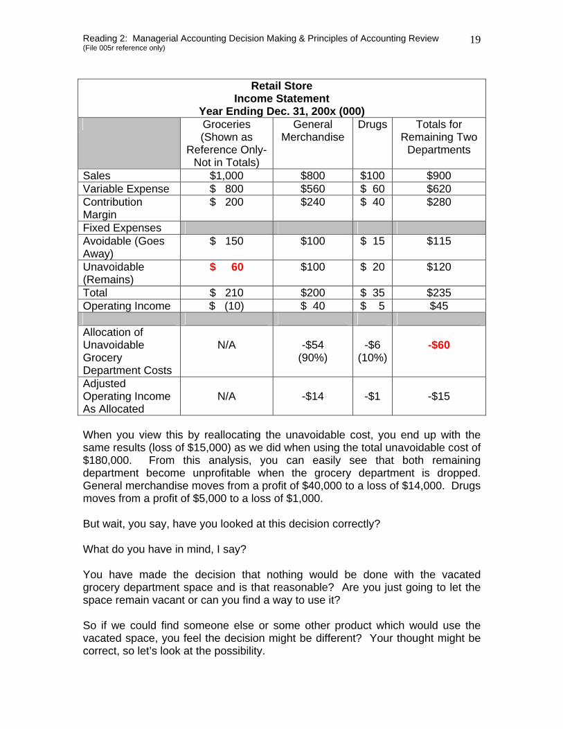
Total $ 210 $200 $ 35 $235 Operating Income $ (10) $ 40 $ 5 $45 Allocation of Unavoidable Grocery Department Costs

N/A

-$54

(90%)

-$6

(10%)

-$60

Adjusted Operating Income As Allocated

N/A

-$14

-$1

-$15

When you view this by reallocating the unavoidable cost, you end up with the same results (loss of $15,000) as we did when using the total unavoidable cost of $180,000. From this analysis, you can easily see that both remaining department become unprofitable when the grocery department is dropped. General merchandise moves from a profit of $40,000 to a loss of $14,000. Drugs moves from a profit of $5,000 to a loss of $1,000. But wait, you say, have you looked at this decision correctly? What do you have in mind, I say? You have made the decision that nothing would be done with the vacated grocery department space and is that reasonable? Are you just going to let the space remain vacant or can you find a way to use it? So if we could find someone else or some other product which would use the vacated space, you feel the decision might be different? Your thought might be correct, so let’s look at the possibility.


20

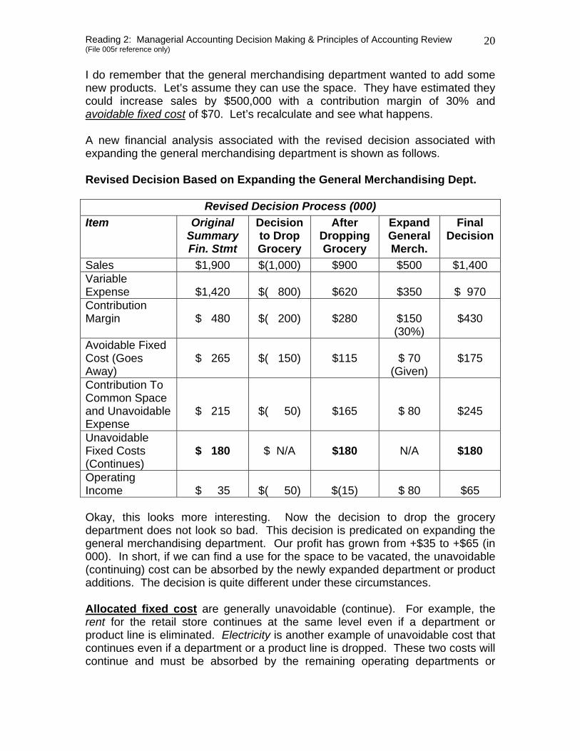
I do remember that the general merchandising department wanted to add some new products. Let’s assume they can use the space. They have estimated they could increase sales by $500,000 with a contribution margin of 30% and avoidable fixed cost of $70. Let’s recalculate and see what happens. A new financial analysis associated with the revised decision associated with expanding the general merchandising department is shown as follows. Revised Decision Based on Expanding the General Merchandising Dept.

Revised Decision Process (000) Item Original

Summary Fin. Stmt

Decision to Drop Grocery

After Dropping Grocery

Expand General Merch.

Final Decision

Sales $1,900 $(1,000) $900 $500 $1,400 Variable Expense

$1,420

$( 800)

$620

$350

$ 970

Contribution Margin

$ 480

$( 200)

$280

$150 (30%)

$430

Avoidable Fixed Cost (Goes Away)

$ 265

$( 150)

$115

$ 70

(Given)

$175

Contribution To Common Space and Unavoidable Expense

$ 215

$( 50)

$165

$ 80

$245

Unavoidable Fixed Costs (Continues)

$ 180

$ N/A

$180

N/A

$180

Operating Income

$ 35

$( 50)

$(15)

$ 80

$65

Okay, this looks more interesting. Now the decision to drop the grocery department does not look so bad. This decision is predicated on expanding the general merchandising department. Our profit has grown from +$35 to +$65 (in 000). In short, if we can find a use for the space to be vacated, the unavoidable (continuing) cost can be absorbed by the newly expanded department or product additions. The decision is quite different under these circumstances. Allocated fixed cost are generally unavoidable (continue). For example, the rent for the retail store continues at the same level even if a department or product line is eliminated. Electricity is another example of unavoidable cost that continues even if a department or a product line is dropped. These two costs will continue and must be absorbed by the remaining operating departments or


21

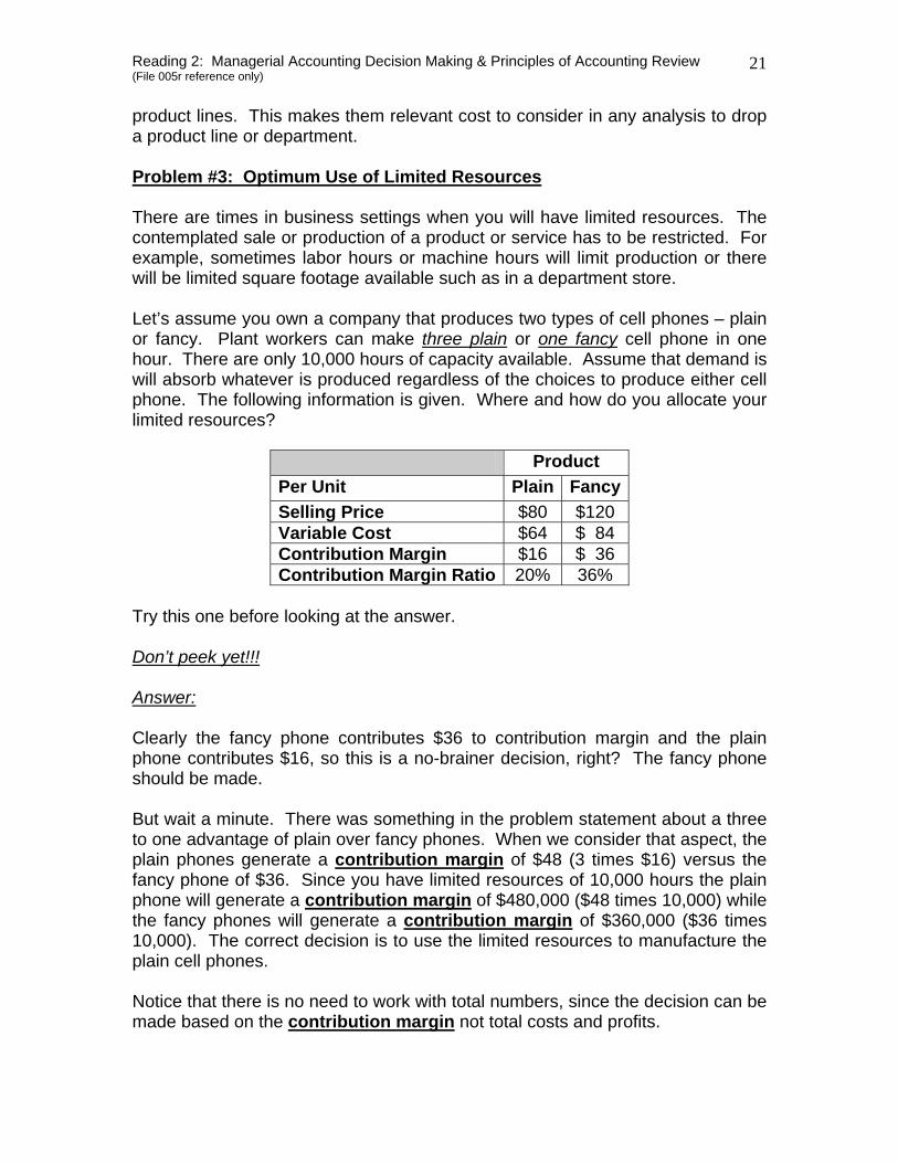
product lines. This makes them relevant cost to consider in any analysis to drop a product line or department. Problem #3: Optimum Use of Limited Resources There are times in business settings when you will have limited resources. The contemplated sale or production of a product or service has to be restricted. For example, sometimes labor hours or machine hours will limit production or there will be limited square footage available such as in a department store. Let’s assume you own a company that produces two types of cell phones – plain or fancy. Plant workers can make three plain or one fancy cell phone in one hour. There are only 10,000 hours of capacity available. Assume that demand is will absorb whatever is produced regardless of the choices to produce either cell phone. The following information is given. Where and how do you allocate your limited resources?

Product Per Unit Plain FancySelling Price $80 $120 Variable Cost $64 $ 84 Contribution Margin $16 $ 36 Contribution Margin Ratio 20% 36%

Try this one before looking at the answer. Don’t peek yet!!! Answer: Clearly the fancy phone contributes $36 to contribution margin and the plain phone contributes $16, so this is a no-brainer decision, right? The fancy phone should be made. But wait a minute. There was something in the problem statement about a three to one advantage of plain over fancy phones. When we consider that aspect, the plain phones generate a contribution margin of $48 (3 times $16) versus the fancy phone of $36. Since you have limited resources of 10,000 hours the plain phone will generate a contribution margin of $480,000 ($48 times 10,000) while the fancy phones will generate a contribution margin of $360,000 ($36 times 10,000). The correct decision is to use the limited resources to manufacture the plain cell phones. Notice that there is no need to work with total numbers, since the decision can be made based on the contribution margin not total costs and profits.


22

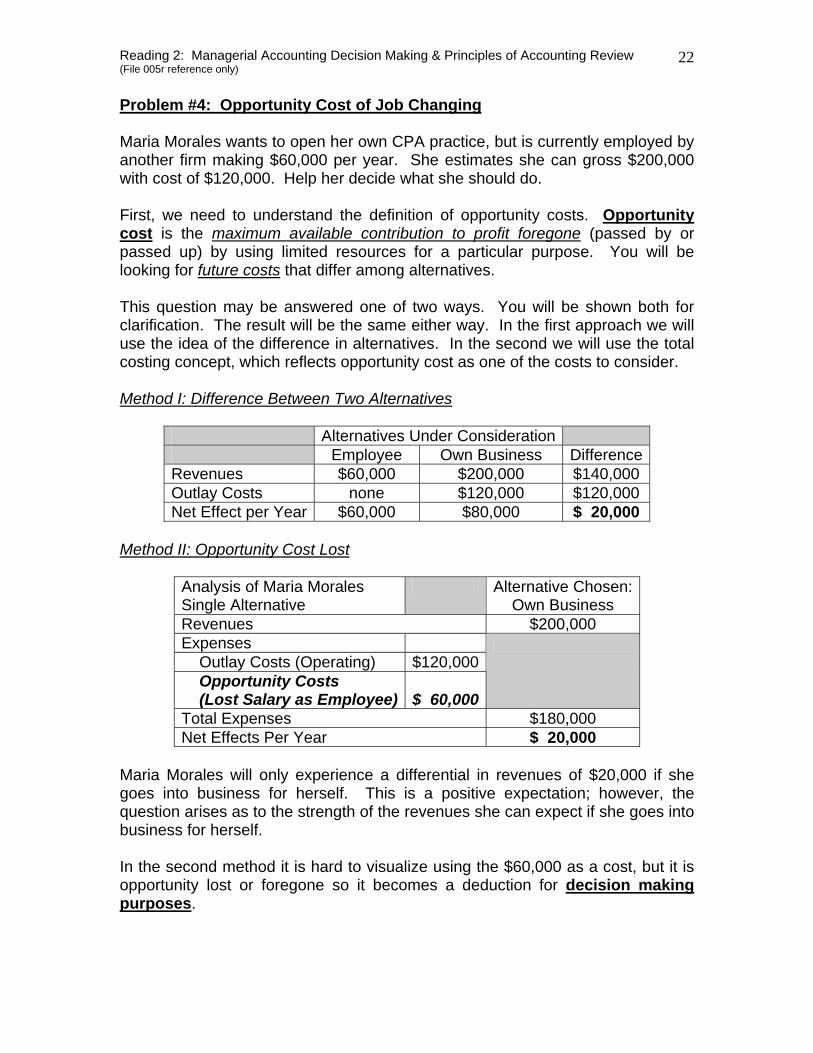
Problem #4: Opportunity Cost of Job Changing Maria Morales wants to open her own CPA practice, but is currently employed by another firm making $60,000 per year. She estimates she can gross $200,000 with cost of $120,000. Help her decide what she should do. First, we need to understand the definition of opportunity costs. Opportunity cost is the maximum available contribution to profit foregone (passed by or passed up) by using limited resources for a particular purpose. You will be looking for future costs that differ among alternatives. This question may be answered one of two ways. You will be shown both for clarification. The result will be the same either way. In the first approach we will use the idea of the difference in alternatives. In the second we will use the total costing concept, which reflects opportunity cost as one of the costs to consider. Method I: Difference Between Two Alternatives

Alternatives Under Consideration Employee Own Business Difference Revenues $60,000 $200,000 $140,000 Outlay Costs none $120,000 $120,000 Net Effect per Year $60,000 $80,000 $ 20,000

Method II: Opportunity Cost Lost

Analysis of Maria Morales Single Alternative

Alternative Chosen: Own Business

Revenues $200,000 Expenses Outlay Costs (Operating) $120,000 Opportunity Costs (Lost Salary as Employee)

$ 60,000

Total Expenses $180,000 Net Effects Per Year $ 20,000

Maria Morales will only experience a differential in revenues of $20,000 if she goes into business for herself. This is a positive expectation; however, the question arises as to the strength of the revenues she can expect if she goes into business for herself. In the second method it is hard to visualize using the $60,000 as a cost, but it is opportunity lost or foregone so it becomes a deduction for decision making purposes.


23

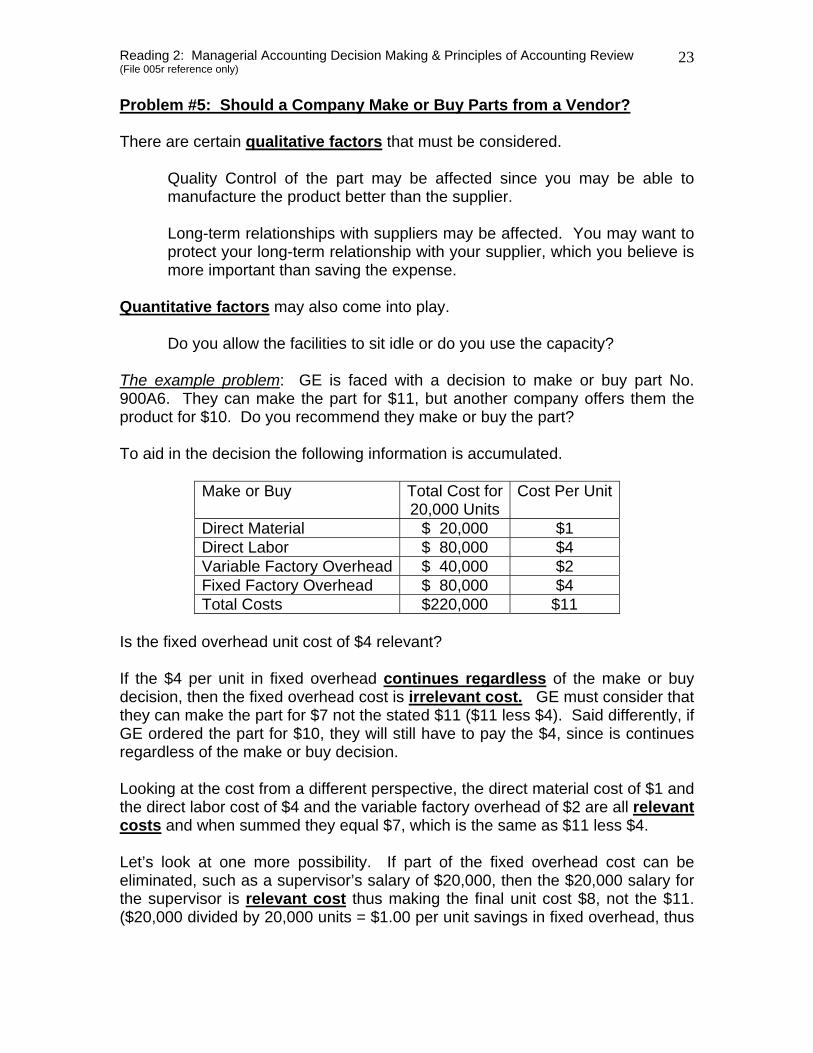
Problem #5: Should a Company Make or Buy Parts from a Vendor? There are certain qualitative factors that must be considered.

Quality Control of the part may be affected since you may be able to manufacture the product better than the supplier.

Long-term relationships with suppliers may be affected. You may want to protect your long-term relationship with your supplier, which you believe is more important than saving the expense.

Quantitative factors may also come into play.

Do you allow the facilities to sit idle or do you use the capacity?

The example problem: GE is faced with a decision to make or buy part No. 900A6. They can make the part for $11, but another company offers them the product for $10. Do you recommend they make or buy the part? To aid in the decision the following information is accumulated.

Make or Buy Total Cost for20,000 Units

Cost Per Unit

Direct Material $ 20,000 $1 Direct Labor $ 80,000 $4 Variable Factory Overhead $ 40,000 $2 Fixed Factory Overhead $ 80,000 $4 Total Costs $220,000 $11

Is the fixed overhead unit cost of $4 relevant? If the $4 per unit in fixed overhead continues regardless of the make or buy decision, then the fixed overhead cost is irrelevant cost. GE must consider that they can make the part for $7 not the stated $11 ($11 less $4). Said differently, if GE ordered the part for $10, they will still have to pay the $4, since is continues regardless of the make or buy decision. Looking at the cost from a different perspective, the direct material cost of $1 and the direct labor cost of $4 and the variable factory overhead of $2 are all relevant costs and when summed they equal $7, which is the same as $11 less $4. Let’s look at one more possibility. If part of the fixed overhead cost can be eliminated, such as a supervisor’s salary of $20,000, then the $20,000 salary for the supervisor is relevant cost thus making the final unit cost $8, not the $11. ($20,000 divided by 20,000 units = $1.00 per unit savings in fixed overhead, thus


24

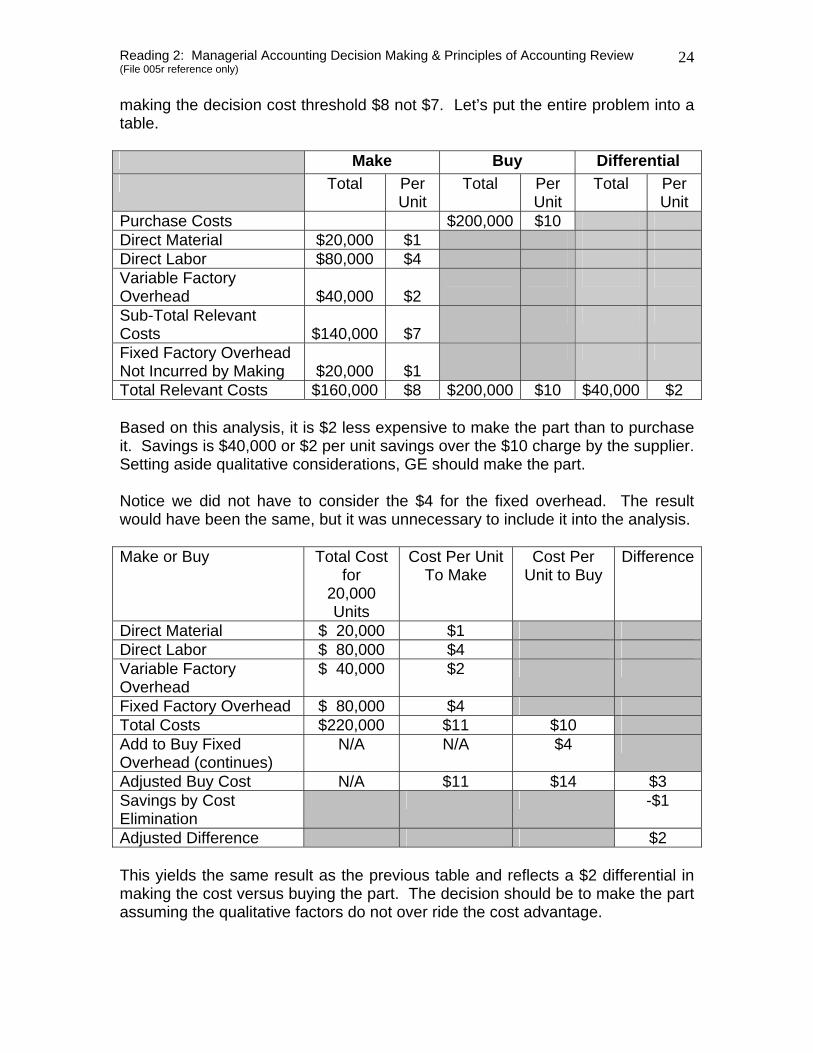
making the decision cost threshold $8 not $7. Let’s put the entire problem into a table. Make Buy Differential Total Per

Unit Total Per

Unit Total Per

Unit Purchase Costs $200,000 $10 Direct Material $20,000 $1 Direct Labor $80,000 $4 Variable Factory Overhead

$40,000

$2

Sub-Total Relevant Costs

$140,000

$7

Fixed Factory Overhead Not Incurred by Making

$20,000

$1

Total Relevant Costs $160,000 $8 $200,000 $10 $40,000 $2 Based on this analysis, it is $2 less expensive to make the part than to purchase it. Savings is $40,000 or $2 per unit savings over the $10 charge by the supplier. Setting aside qualitative considerations, GE should make the part. Notice we did not have to consider the $4 for the fixed overhead. The result would have been the same, but it was unnecessary to include it into the analysis. Make or Buy Total Cost

for 20,000 Units

Cost Per Unit To Make

Cost Per Unit to Buy

Difference

Direct Material $ 20,000 $1 Direct Labor $ 80,000 $4 Variable Factory Overhead

$ 40,000 $2

Fixed Factory Overhead $ 80,000 $4 Total Costs $220,000 $11 $10 Add to Buy Fixed Overhead (continues)

N/A N/A $4

Adjusted Buy Cost N/A $11 $14 $3 Savings by Cost Elimination

-$1

Adjusted Difference $2 This yields the same result as the previous table and reflects a $2 differential in making the cost versus buying the part. The decision should be to make the part assuming the qualitative factors do not over ride the cost advantage.


25

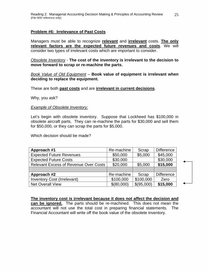
Problem #6: Irrelevance of Past Costs Managers must be able to recognize relevant and irrelevant costs. The only relevant factors are the expected future revenues and costs. We will consider two types of irrelevant costs which are important to consider. Obsolete Inventory - The cost of the inventory is irrelevant to the decision to move forward to scrap or re-machine the parts. Book Value of Old Equipment – Book value of equipment is irrelevant when deciding to replace the equipment. These are both past costs and are irrelevant in current decisions. Why, you ask? Example of Obsolete Inventory: Let’s begin with obsolete inventory. Suppose that Lockheed has $100,000 in obsolete aircraft parts. They can re-machine the parts for $30,000 and sell them for $50,000, or they can scrap the parts for $5,000. Which decision should be made? Approach #1 Re-machine Scrap DifferenceExpected Future Revenues $50,000 $5,000 $45,000 Expected Future Costs $30,000 $30,000 Relevant Excess of Revenue Over Costs $20,000 $5,000 $15,000 Approach #2 Re-machine Scrap Difference Inventory Cost (Irrelevant) $100,000 $100,000 Zero Net Overall View $(80,000) $(95,000) $15,000 The inventory cost is irrelevant because it does not affect the decision and can be ignored. The parts should be re-machined. This does not mean the accountant will not use the total cost in preparing financial statements. The Financial Accountant will write off the book value of the obsolete inventory.


26

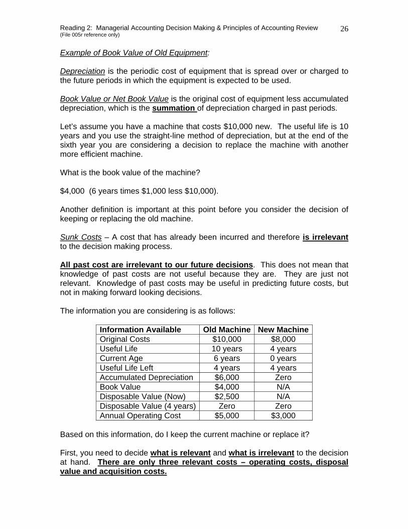
Example of Book Value of Old Equipment: Depreciation is the periodic cost of equipment that is spread over or charged to the future periods in which the equipment is expected to be used. Book Value or Net Book Value is the original cost of equipment less accumulated depreciation, which is the summation of depreciation charged in past periods. Let’s assume you have a machine that costs $10,000 new. The useful life is 10 years and you use the straight-line method of depreciation, but at the end of the sixth year you are considering a decision to replace the machine with another more efficient machine. What is the book value of the machine? $4,000 (6 years times $1,000 less $10,000). Another definition is important at this point before you consider the decision of keeping or replacing the old machine. Sunk Costs – A cost that has already been incurred and therefore is irrelevant to the decision making process. All past cost are irrelevant to our future decisions. This does not mean that knowledge of past costs are not useful because they are. They are just not relevant. Knowledge of past costs may be useful in predicting future costs, but not in making forward looking decisions. The information you are considering is as follows:

Information Available Old Machine New Machine Original Costs $10,000 $8,000 Useful Life 10 years 4 years Current Age 6 years 0 years Useful Life Left 4 years 4 years Accumulated Depreciation $6,000 Zero Book Value $4,000 N/A Disposable Value (Now) $2,500 N/A Disposable Value (4 years) Zero Zero Annual Operating Cost $5,000 $3,000

Based on this information, do I keep the current machine or replace it? First, you need to decide what is relevant and what is irrelevant to the decision at hand. There are only three relevant costs – operating costs, disposal value and acquisition costs.


27

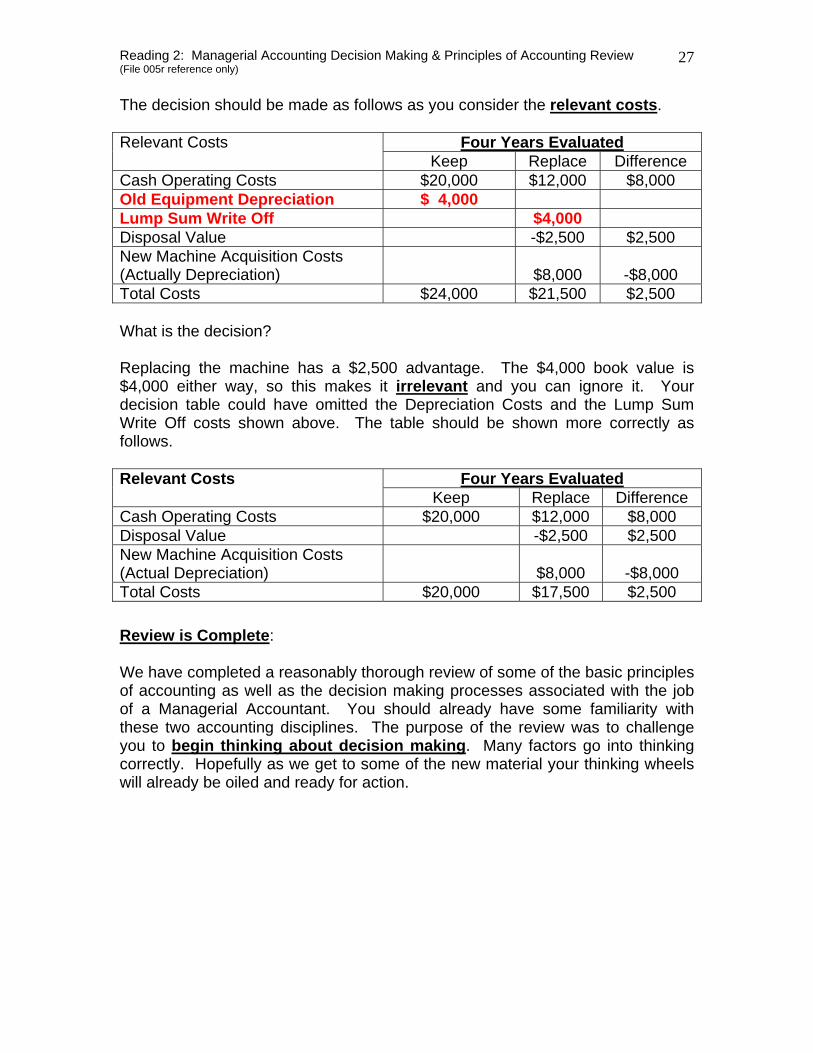
The decision should be made as follows as you consider the relevant costs.

Four Years EvaluatedRelevant Costs Keep Replace Difference

Cash Operating Costs $20,000 $12,000 $8,000 Old Equipment Depreciation $ 4,000 Lump Sum Write Off $4,000 Disposal Value -$2,500 $2,500 New Machine Acquisition Costs (Actually Depreciation)

$8,000

-$8,000

Total Costs $24,000 $21,500 $2,500 What is the decision? Replacing the machine has a $2,500 advantage. The $4,000 book value is $4,000 either way, so this makes it irrelevant and you can ignore it. Your decision table could have omitted the Depreciation Costs and the Lump Sum Write Off costs shown above. The table should be shown more correctly as follows.

Four Years EvaluatedRelevant Costs Keep Replace Difference

Cash Operating Costs $20,000 $12,000 $8,000 Disposal Value -$2,500 $2,500 New Machine Acquisition Costs (Actual Depreciation)

$8,000

-$8,000

Total Costs $20,000 $17,500 $2,500 Review is Complete: We have completed a reasonably thorough review of some of the basic principles of accounting as well as the decision making processes associated with the job of a Managerial Accountant. You should already have some familiarity with these two accounting disciplines. The purpose of the review was to challenge you to begin thinking about decision making. Many factors go into thinking correctly. Hopefully as we get to some of the new material your thinking wheels will already be oiled and ready for action.

principles of accounting review - dallas baptist...

Documents