principal component estimation of …hera.ugr.es/doi/15057823.pdfprincipal component estimation of...

Nonparametric StatisticsVol. 16(3–4), June–August 2004, pp. 365–384

PRINCIPAL COMPONENT ESTIMATION OFFUNCTIONAL LOGISTIC REGRESSION: DISCUSSION

OF TWO DIFFERENT APPROACHES

M. ESCABIAS∗, A. M. AGUILERA and M. J. VALDERRAMA

Department of Statistics and Operation Research, University of Granada, Spain

(Received 14 December 2002; Revised 21 July 2003; In final form 10 September 2003)

Over the last few years many methods have been developed for analyzing functional data with different objectives. Thepurpose of this paper is to predict a binary response variable in terms of a functional variable whose sample informationis given by a set of curves measured without error. In order to solve this problem we formulate a functional logisticregression model and propose its estimation by approximating the sample paths in a finite dimensional space generatedby a basis. Then, the problem is reduced to a multiple logistic regression model with highly correlated covariates. Inorder to reduce dimension and to avoid multicollinearity, two different approaches of functional principal componentanalysis of the sample paths are proposed. Finally, a simulation study for evaluating the estimating performance ofthe proposed principal component approaches is developed.

Keywords: Functional data analysis; Logistic regression; Principal components

1 INTRODUCTION

Data in many different fields come to us through a process naturally described as functions.This is the case of the evolution of a magnitude such as, for example, temperature in time.It usually happens that we only have discrete observations of functional data in spite of itscontinuous nature. In order to reconstruct the true functional form of data many approximationtechniques have been developed, such as interpolation or smoothing in a finite dimensionalspace generated by a basis. A general overview of functional data analysis (FDA) can be seenin Ramsay and Silverman (1997, 2002) and Valderrama et al. (2000).

The great development on FDA in recent years has meant that many studies with longi-tudinal data historically raised from a multiple point of view are now analyzed on the basisof their functional nature. Some of these works have focused on modeling the relationshipbetween functional predictor and response variables observed together at varying times. Thisis the case for example, in Liang and Zeger (1986) who proposed a set of estimating equationswhich take into account the correlation between discrete longitudinal observations in order toestimate a set of time-independent parameters in the generalized linear model context. Withthe objective of estimating a functional variable in a future period of time from its past evo-lution, Aguilera et al. (1997a) introduced the principal component prediction models (PCP)

∗ Corresponding author. E-mail: [email protected]

ISSN 1048-5252 print; ISSN 1029-0311 online c© 2004 Taylor & Francis LtdDOI: 10.1080/10485250310001624738

366 M. ESCABIAS et al.

that have been adapted for forecasting a continuous-time series based on discrete observa-tions at unequally spaced time points (Aguilera et al., 1999a, b). More recently, Valderramaet al. (2002) have formulated mixed ARIMA-PCP models to solve a related problem.

On the other hand, in many practical situations it is necessary to model the relationshipbetween a time-independent response and a functional predictor. A first approach to functionallinear regression has been introduced by Ramsay and Silverman (1997) for the case of acontinuous scalar response variable and the functional predictor measured at the same timepoints for each individual. When the response variable is the own functional predictor in afuture time point, Aguilera et al. (1997b) proposed a principal component (PC) approach tofunctional linear regression.

The aim of this work is to predict a binary response variable, or equivalently the probabilityof occurrence of an event, from the evolution of a continuous variable in time, so that functionalinformation is provided by a set of sample paths. This is the case in Ratcliffe et al. (2002),who used periodically stimulated foetal heart rate tracings to predict the probability of a highrisk birth outcome. Taking into account that the analysis of such phenomenon has to be doneby looking at its continuous nature we propose a functional regression model. On the otherhand linear models are not the best ones when the response variable is binary as stated byHosmer and Lemeshow (1989) in the multiple case, therefore we develop a functional logisticregression model.

As Ramsay and Silverman (1997) stated for the case of functional linear models, the esti-mation of such a model cannot be obtained by the usual methods of least squares or maxi-mum likelihood. In the general context of generalized functional linear models, James (2002)assumes that each predictor can be modeled as a smooth curve from a given functional familyas for example, natural cubic splines. Then the functional model can be equivalently seen as ageneralized linear model whose design matrix is given by the unobserved spline basis coeffi-cients for the predictor and the EM algorithm is used for estimating the model from longitudinalobservations at different times for each individual. In order to assess the relationship betweenthe functional predictor and the scalar response, either estimating the parameter function byconsidering an orthonormal spline basis or using as covariates all the PCs of the spline basiscoefficients is also performed. In an unpublished paper, Muller and Stadmuller (2002) proposean estimation based on truncating an infinite basis expansion of the functional predictor whosesample curves are assumed to be in the space of square integrable functions. In that paper,asymptotic inference for the proposed class of generalized regression models is developed byusing the orthonormal basis of eigenfunctions of the covariance function.

In this line of research the present paper provides some alternative methods for estimatingthe parameter function in the functional logistic regression model. A first estimation procedureis obtained by assuming that both the functional predictor and the parameter function belongto a finite space generated by a basis of functions that could be unorthonormal. Opposite toJames (2002) that assumes unknown basis coefficients we fit a separate curve to each individualand approximate its basis coefficients from its observations at different time points. Then anapproximated estimation is performed by estimating a standard multiple logistic regressionmodel whose design matrix is the product of the matrix of resulting basis coefficients andthe one of inner products between basis functions. This results in highly correlated covariates(multicollinearity) which causes the model to be unstable, as indicated by Ryan (1997), so thatthe parameter estimates provided by most statistical packages are not particularly accurate.To solve this problem in multiple logistic regression Aguilera and Escabias (2000) proposedto use a reduced set of PCs of the original predictor variables as covariates of the model and toobtain an estimation of the original parameters through the one provided by this PC logisticregression model. In order to reduce dimension and to avoid multicollinearity, in this paperwe propose a second estimation procedure based on functional principal component analysis

PRINCIPAL COMPONENT ESTIMATION OF FUNCTIONAL LOGISTIC REGRESSION 367

(FPCA) of the original sample paths to improve the approximated estimation of the parameterfunction obtained when we consider that the sample paths and the parameter function belongto the same finite-dimension space.

Summarizing, the main advantage of this paper with respect to previous works in this areais to propose an estimation procedure of functional logistic regression, based on taking ascovariates a reduced set of functional principal components of the predictor sample paths aftertheir approximation on a finite space generated by a basis of no necessarily orthonormalfunctions. This is in contrast to the particular case of the orthonormal bases used in other papers,when the basis is unorthonormal standard FPCA is not equivalent to principal componentanalysis (PCA) of the resulting basis coefficients so that two different approaches to FPCAwill be considered. Then their estimating performance will be evaluated on simulated data byproposing different criterions and some heuristic guidelines for choosing the optimal PCs tobe included as covariates in the resulting functional PCs logistic regression model.

In Section 2, we briefly present the general ideas about how to reconstruct the true functionalform of data by fitting a smooth curve to each individual from its observations at different times.Basic theory on FPCA is also summarized with special emphasis on the case of predictorcurves in a finite space generated by a basis. The theoretical framework on functional logisticregression and a first estimation procedure based on approximating the basis coefficients ofpredictor curves on a finite space are developed in Section 3. In order to avoid multicollinearity,in Section 4 we propose a second estimation procedure for functional logistic regression thatuses as covariates a reduced set of functional principal components of the predictor curves.Two different forms of FPCA and two different criterions for including the covariates in themodel will be also considered. Simulation studies for testing the accuracy of the parameterfunction provided by these functional PC approaches are finally carried out in Section 5.

2 FUNCTIONAL DATA

The aim of this paper is to explain a binary response variable in terms of a functional predictorwhose sample information is given by a set of functions x1(t), x2(t), . . . , xn(t) that can beseen as observations of a stochastic process {X (t): t ∈ T }. From now on, we will suppose thatthis stochastic process is second order, continuous in quadratic mean and the sample functionsbelong to the Hilbert space L2(T ) of squared integrable functions, with the usual inner product

〈 f, g〉u =∫

Tf (t)g(t) dt, ∀ f, g ∈ L2(T ).

In practice it is impossible to observe a set of functions continuously in time: instead wewill usually have observations of such functions at different times, ti0, ti1, . . . , timi ∈ T, i =1, . . . , n, and with a different number of observations for each individual. That is, the sampleinformation is given by the vectors xi = (xi0, . . . , ximi )

′, with xik being the observed value ofthe i th sample path at time tik(k = 0, . . . ,mi).

In order to reconstruct the functional form of sample paths from the discrete observedinformation we may use different methods depending on the way of obtaining such discrete-time data and the shape we expect the functions to have. In any case, it is usual to assume thatsample paths belong to a finite-dimension space generated by a basis {φ1(t), . . . , φp(t)}, sothat they can be expressed as

xi(t) =p∑

j=1

ai jφj(t), i = 1, . . . , n. (1)


If the functional predictor is observed with error

xik = xi(tik)+ εk k = 0, . . . ,mi ,

we can use some least square approximation approach after choosing a suitable basis as, forexample, trigonometric functions (Aguilera et al., 1995), B-splines or wavelets (see Ramsayand Silverman, 1997 for a detailed study). On the other hand if we consider that sample curvesare observed without error

xik = xi(tik) k = 0, . . . ,mi ,

we could use some interpolation method, as for example, cubic spline interpolation (Aguileraet al., 1996).

Both methods, smoothing and interpolation, allow us to obtain the functional form of thesample paths by approximating the basis coefficients {ai j} from the discrete-time observationsof sample curves.

The different methods that we will propose later for estimating the functional logistic regres-sion model are based on FPCA, so let us briefly look at the basic theory on functional PCs.

2.1 Functional Principal Component Analysis

We are going to define FPCA from a sample point of view. By analogy with multivariate case,the functional PCs of a stochastic process are defined as uncorrelated generalized linear spanof its variables with maximum variance.

Let x1(t), . . . , xn(t) ∈ L2(T ) be a set of sample paths of a continuous stochastic process{X (t): t ∈ T }. The sample mean and covariance functions are given by

x(t) = 1

n

n∑i=1

xi(t)

C(s, t) = 1

n − 1

n∑i=1

(xi(s)− x(s))(xi (t)− x(t)).

We will consider without loss of generality that x(t) = 0 ∀t ∈ T .The functional PCs of x1(t), . . . , xn(t) are defined as n-dimensional vectors ξj ( j =

1, . . . , n − 1) with components

ξi j =∫

Txi(t) f j (t) dt, i = 1, . . . , n,

where the weight functions f j (t) that define the functional PCs are the n − 1 solutions of theeigenproblem ∫

TC(s, t) f (s) ds = λ f (t), ∀t ∈ T . (2)

That is, f j(t) ( j = 1, . . . , n − 1) are the eigenfunctions associated to the corresponding positiveeigenvalues λj ( j = 1, . . . , n − 1) that are the variances of the PCs and verify λ1 >

λ2 > · · · > λn−1 ≥ 0.


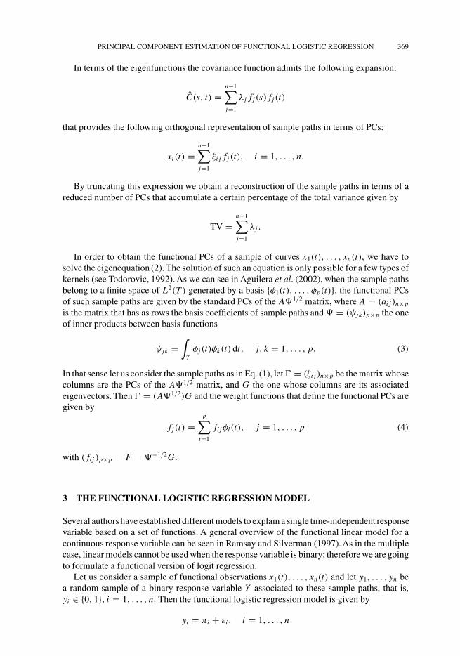
In terms of the eigenfunctions the covariance function admits the following expansion:

C(s, t) =n−1∑j=1

λj f j (s) f j(t)

that provides the following orthogonal representation of sample paths in terms of PCs:

xi(t) =n−1∑j=1

ξi j f j (t), i = 1, . . . , n.

By truncating this expression we obtain a reconstruction of the sample paths in terms of areduced number of PCs that accumulate a certain percentage of the total variance given by

TV =n−1∑j=1

λj .

In order to obtain the functional PCs of a sample of curves x1(t), . . . , xn(t), we have tosolve the eigenequation (2). The solution of such an equation is only possible for a few types ofkernels (see Todorovic, 1992). As we can see in Aguilera et al. (2002), when the sample pathsbelong to a finite space of L2(T ) generated by a basis {φ1(t), . . . , φp(t)}, the functional PCsof such sample paths are given by the standard PCs of the A�1/2 matrix, where A = (ai j)n×p

is the matrix that has as rows the basis coefficients of sample paths and� = (ψjk)p×p the oneof inner products between basis functions

ψjk =∫

Tφj(t)φk(t) dt, j, k = 1, . . . , p. (3)

In that sense let us consider the sample paths as in Eq. (1), let� = (ξi j )n×p be the matrix whosecolumns are the PCs of the A�1/2 matrix, and G the one whose columns are its associatedeigenvectors. Then � = (A�1/2)G and the weight functions that define the functional PCs aregiven by

f j(t) =p∑

t=1

fl jφl(t), j = 1, . . . , p (4)

with ( fl j )p×p = F = �−1/2G.

3 THE FUNCTIONAL LOGISTIC REGRESSION MODEL

Several authors have established different models to explain a single time-independent responsevariable based on a set of functions. A general overview of the functional linear model for acontinuous response variable can be seen in Ramsay and Silverman (1997). As in the multiplecase, linear models cannot be used when the response variable is binary; therefore we are goingto formulate a functional version of logit regression.

Let us consider a sample of functional observations x1(t), . . . , xn(t) and let y1, . . . , yn bea random sample of a binary response variable Y associated to these sample paths, that is,yi ∈ {0, 1}, i = 1, . . . , n. Then the functional logistic regression model is given by

yi = πi + εi , i = 1, . . . , n


where πi is the expectation of Y given xi(t) that will be modelized as

πi = P[Y = 1|{xi(t): t ∈ T }]

= exp{α + ∫T xi(t)β(t) dt}

1 + exp{α + ∫T xi(t)β(t) dt} , i = 1, . . . , n

with α a real parameter, β(t) a parameter function, and εi , i = 1, . . . , n independent errorswith zero mean.

Equivalently the logit transformations can be expressed as

li = ln

[πi

1 − πi

]= α +

∫T

xi(t)β(t) dt, i = 1, . . . , n, (5)

where T is the support of the sample paths xi(t). So the functional logistic regression model canbe seen as a functional generalized linear model with the logit transformation as link function(James, 2002).

As indicated by Ramsay and Silverman (1997) for the functional linear regression model, itis impossible to obtain an estimation of β(t) by the usual methods of least squares or maximumlikelihood. As we stated earlier, in order to solve this problem we will assume that both samplepaths and parameter function belong to the same finite space.

3.1 An Approximated Estimation of the Parameter Function

Let us consider the sample paths as in Eq. (1), and the parameter function in terms of the samebasis,

β(t) =p∑

k=1

βkφk(t).

Once the basis coefficients of sample curves have been approximated from discrete-time data,their resulting approximated basis representations turn the functional model into a multipleone

li = α +∫

Txi(t)β(t) dt = α +

p∑j=1

p∑k=1

ai jψjkβk, i = 1, . . . , n

with ψjk the inner products defined in Eq. (3), ai j the coordinates of sample paths, α a scalarparameter and βk the parameters of the model that correspond to the parameter function basiscoefficients which have to be estimated. In matrix form this multiple model can be expressedas

L = α1 + A�β, (6)

where A=(ai j)n×p,�=(ψjk)p×p, β=(β1, . . . , βp)′, 1=(1, . . . , 1)′ and L =(l1, . . . , ln)

′.Then, we will obtain an estimation of the parameter function by estimating this multiple

logistic model. So let β = (β1, . . . , βp)′ the estimated parameters of this multiple model

obtained by applying the Newton-Raphson method for solving the nonlinear likelihoodequations

X ′(Y −�) = 0,


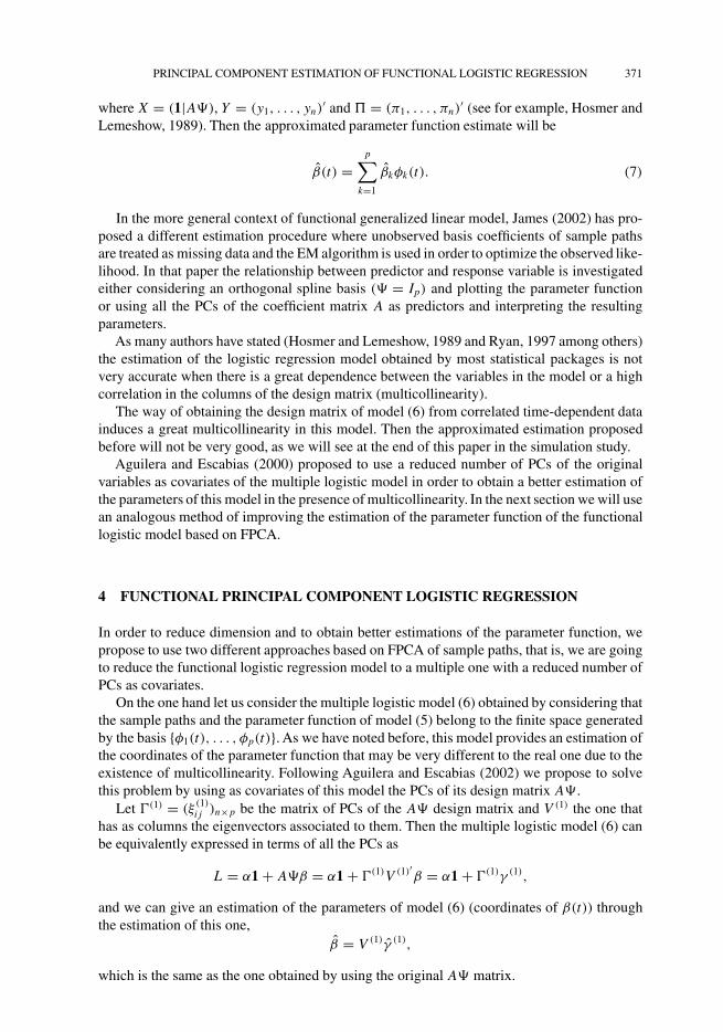
where X = (1|A�), Y = (y1, . . . , yn)′ and� = (π1, . . . , πn)

′ (see for example, Hosmer andLemeshow, 1989). Then the approximated parameter function estimate will be

β(t) =p∑

k=1

βkφk(t). (7)

In the more general context of functional generalized linear model, James (2002) has pro-posed a different estimation procedure where unobserved basis coefficients of sample pathsare treated as missing data and the EM algorithm is used in order to optimize the observed like-lihood. In that paper the relationship between predictor and response variable is investigatedeither considering an orthogonal spline basis (� = Ip) and plotting the parameter functionor using all the PCs of the coefficient matrix A as predictors and interpreting the resultingparameters.

As many authors have stated (Hosmer and Lemeshow, 1989 and Ryan, 1997 among others)the estimation of the logistic regression model obtained by most statistical packages is notvery accurate when there is a great dependence between the variables in the model or a highcorrelation in the columns of the design matrix (multicollinearity).

The way of obtaining the design matrix of model (6) from correlated time-dependent datainduces a great multicollinearity in this model. Then the approximated estimation proposedbefore will not be very good, as we will see at the end of this paper in the simulation study.

Aguilera and Escabias (2000) proposed to use a reduced number of PCs of the originalvariables as covariates of the multiple logistic model in order to obtain a better estimation ofthe parameters of this model in the presence of multicollinearity. In the next section we will usean analogous method of improving the estimation of the parameter function of the functionallogistic model based on FPCA.

4 FUNCTIONAL PRINCIPAL COMPONENT LOGISTIC REGRESSION

In order to reduce dimension and to obtain better estimations of the parameter function, wepropose to use two different approaches based on FPCA of sample paths, that is, we are goingto reduce the functional logistic regression model to a multiple one with a reduced number ofPCs as covariates.

On the one hand let us consider the multiple logistic model (6) obtained by considering thatthe sample paths and the parameter function of model (5) belong to the finite space generatedby the basis {φ1(t), . . . , φp(t)}. As we have noted before, this model provides an estimation ofthe coordinates of the parameter function that may be very different to the real one due to theexistence of multicollinearity. Following Aguilera and Escabias (2002) we propose to solvethis problem by using as covariates of this model the PCs of its design matrix A� .

Let �(1) = (ξ(1)i j )n×p be the matrix of PCs of the A� design matrix and V (1) the one that

has as columns the eigenvectors associated to them. Then the multiple logistic model (6) canbe equivalently expressed in terms of all the PCs as

L = α1 + A�β = α1 + �(1)V (1)′β = α1 + �(1)γ (1),

and we can give an estimation of the parameters of model (6) (coordinates of β(t)) throughthe estimation of this one,

β = V (1)γ (1),

which is the same as the one obtained by using the original A� matrix.


This PCA is really a FPCA of a transformation of the original sample paths with respectto the usual inner product in L2(T ). In fact, Aguilera et al. (2002) have proved that thistransformation is given by U(xi)(t) = ′�1/2a′

i with ai = (ai1, . . . , aip)′ being the i th row of

A and = (φ1(t), . . . , φp(t))′.On the other hand, let us denote by �(2) = (ξ

(2)i j )n×p the matrix of functional PCs of

x1(t), . . . , xn(t) obtained as in Section 2.1; then we can express

xi(t) =p∑

j=1

ξ(2)i j f j (t), i = 1, . . . , n

and model (5) can be equivalently expressed as

li = α +p∑

j=1

ξ(2)i j γ

(2)j , i = 1, . . . , n,

with

γ(2)j =

∫T

fj (t)β(t) dt, j = 1, . . . , p.

Equivalently, if we consider the multiple logistic model in terms of these PCs

li = α +p∑

j=1

ξ(2)i j γ

(2)j = α +

p∑j=1

(∫T

xi(t) f j (t) dt

)γ(2)j

= α +∫

Txi(t)

p∑

j=1

f j (t)γ(2)j

dt, i = 1, . . . , n,

we obtain the following expression for the parameter function

β(t) =p∑

j=1

f j(t)γ(2)j .

Under these considerations, we can obtain an estimation of the parameter function byestimating the multiple model in terms of all PCs and substituting f j (t), j = 1, . . . , p with itsbasis expansion (4). Then its basis coefficients are given by

βj =p∑

l=1

fl j γ(2)j , j = 1, . . . , p

and ( fl j )p×p = F defined in Section 2.1 in terms of the eigenvectors of the covariance matrixof A�1/2. In matrix form β = F γ (2) = �−1/2Gγ (2).

Summarizing, we have proved that the functional logistic regression model (5) can beequivalently expressed as

li = α +p∑

j=1

ξ(k)i j γ

(k)j , i = 1, . . . , n, k = 1, 2, (8)


where the functional PCs ξ (k)j (k = 1, 2) can be obtained by the following two differentapproaches:

1. Performing PCA of the design matrix A� of the multiple logistic model (6) with respect tothe usual inner product in R

p that is equivalent to FPCA of a transformation of the samplepaths with respect to the usual inner product in L2(T ), that is, �(1) = A�V (1). We will callthis principal component analysis PCA1.

2. Performing FPCA of the sample paths with respect to the usual inner product in L2(T ) thatis equivalent to PCA of the data matrix A�1/2, that is �(2) = A�1/2G. We will call thisprincipal component analysis PCA2.

In any case, an estimation of the parameter function can be given by

β(t) =p∑

j=1

βjφj(t) = β ′ , (9)

where the vector of coordinates β = V (k)γ (k) (k = 1, 2), with V (1) the matrix whose columnsare the eigenvectors of the covariance matrix of A� and V (2) = F�−1/2G, with G being thematrix whose columns are the eigenvectors of the covariance matrix of A�1/2.

Let us observe that both approaches agree when the basis is orthonormal and then� = Ip.

4.1 Model Formulation

The functional principal component logistic regression model is obtained by truncating model(8) in terms of a subset of PCs. Then, if we consider the matrices defined before partitioned asfollows:

�(k) = (�(k)(s) | �(k)(r) ), V (k) = (V (k)

(s) | V (k)(r) ), r + s = p, k = 1, 2

the functional principal component logistic regression model is defined by taking as covariatesthe first s PCs

L(k)(s) = α(k)(s)1 + �

(k)(s) γ

(k)(s) , k = 1, 2,

where α(k)(s) is a real parameter and L(k)(s) = (l(k)1(s), . . . , l(k)n(s))with l(k)i(s) = ln[π(k)i(s)/(1 − π

(k)i(s))], and

π(k)i(s) = exp{α(k)(s) + ∑s

j=1 ξ(k)i j γ

(k)j (s)}

1 + exp{α(k)(s) + ∑sj=1 ξ

(k)i j γ

(k)j (s)}

, i = 1, . . . , n, k = 1, 2. (10)

It will be seen in the simulation study that the estimation of the parameter function given by

β(k)(s) (t) =

p∑j=1

β(k)j (s)φj(t) = β

(k)′(s) , k = 1, 2 (11)

with the coefficient vector β(k)(s) = V (k)(s) γ

(k)(s) is more accurate than the one obtained with the

original A� design matrix.


4.2 Model Selection

In spite of having included the PCs in the model according to explained variability, severalauthors, for example Hocking (1976), in PC regression, have established that PCs must beincluded based on a different criterion by taking into account their predictive ability.AsAguileraand Escabias (2000) established for the multiple case, it is better to include the PCs in themodel in the order given by the stepwise method based on conditional likelihood ratio test.In the context of generalized linear models, Muller and Stadmuller (2002) select the numberof predictors (base functions) in a sequence of nested models by using the standard AkaikeInformation Criterion (AIC) and the Bayesian Information Criterion (BIC).

In the simulation study performed at the end of this paper we will consider two differentmethods of including PCs in the model. The first one (Method I) consists of including PCsin the natural order given by the explained varability. In the second one (Method II) PCs areincluded in the order given by the stepwise method based on conditional likelihood ratio test.This method consists of a stepwise procedure of including variables (PCs) into a regressionmodel. Each step of the method tests whether each of the available variables ought to be in thepresent model by the likelihood ratio test for selecting one between two nested models: theones with and without the corresponding variable. The procedure begins with the model withno variables.

In addition we will propose different criterions for selecting the optimal number of PCs basedon different accuracy measures of the estimated parameters. First, we define the integrated meansquared error of the beta parameter function (IMSEB) as

IMSEB(k)(s) = 1

T

∫T(β(t)—β

(k)(s) (t))

2 dt

= 1

T(β − β

(k)(s) )

′�(β − β(k)(s) ) k = 1, 2.

Second, we define the mean squared error of beta parameters (MSEB)

MSEB(k)(s) = 1

p + 1

(α − α

(k)(s) )

2 +p∑

j=1

(βj − β(k)j (s))

2

, k = 1, 2.

Let us observe that mean squared errors provide a good estimation when they are small enough.Therefore, in order to select the optimum number of PCs we will propose two optimum modelsfor each method: the one with the smallest MSEB and the one with the smallest IMSEB.

We have to note that we cannot obtain IMSEB and MSEB with real data, in which case weneed another measure that chooses the best estimation of the parameter function. In literature wecan see several methods of choosing the best number of covariates to estimate the parameter ofa regression model, some of which take into account the values of the variance of the estimatedparameters (see for example Aucott et al. 2000). This variance of the estimated parameters isgiven in functional principal component logistic regression by

var(k)(s) = var[β(k)(s) ] = V (k)′(s) (�

(k)′(s) W (k)

(s) �(k)(s) )

−1V (k)(s) , k = 1, 2,

where W (k)(s) = diag(π (k)i(s)(1 − π

(k)i(s))). We have observed in the simulated examples that

the model previous to a significant increase in this variance provides a good estimation ofthe parameter function with mean squared errors similar to the optimum models. Then wewill use this criterion for model selection in applications with real data. As heuristic rule forchoosing the model with the variance criterion we propose to plot the variances and retain in


the model the PCs previous to a kink in the curve. In addition we will take into account theparsimonious criterion so that between two significant increases in the variances we prefer themodel with less PCs.

5 SIMULATION STUDY

In order to investigate the improvement in the parameter function estimation of the functionallogistic regression model provided by the two proposed PC approaches, we have carried out asimulation study.

5.1 Simulation Process and Model Fitting

We have performed two simulations with the same drawing and a different procedure of samplecurves simulation. Due to the fact that all presented methods consider that sample paths belongto a finite space generated by a basis, we have used the space of cubic splines generated by abasis of cubic B-splines defined by a set of nodes.

Before developing the simulated study let us briefly see the definition of the B-spline basisgiven by a set of nodes t0 < t1 < · · · < tm . Extending this partition as t−3 < t−2 < t−1 < t0 <· · · < tm < tm+1 < tm+2 < tm+3 the B-spline basis is recursively defined by

Bj,1(t) =

1 tj−2 < t < tj−1

0 t /∈ (tj−2, tj−1), j = −1, . . . ,m + 3

Bj,r(t) = t − tj−2

tj+r−3 − tj−2Bj,r−1(t)+ tj+r−2 − t

tj+r−2 − tj−1Bj+1,r−1(t),

r = 2, 3, 4, j = −1, . . . ,m − r + 5

(more details in De Boor 1978). From now we will omit the subscript corresponding to thedegree of cubic B-spline functions (r = 4).

The first step of the simulation process in each case was to have a set of n sample curves thatwill explain the response. These curves are considered in the form (1) in terms of the basic cubicB-splines and their basis coefficients (A matrix). In the first example we have directly simulatedthese coefficients. In the second we have approximated them by least squares approximationfrom a set of observations of a known stochastic process simulated at a finite set of times.

After this we have chosen as parameter functions in the two examples the natural cubicspline interpolation of a known function on the set of nodes of definition of B-splines. Thenthe real basis coefficients β = (β1, . . . , βp)

′ of the parameter function are known.Finally we have obtained the values of the response variable Y by simulating the functional

logistic regression model. That is, first we have obtained the linear spans

ci =∫

Txi(t)β(t) dt = a′

i�β, 1, . . . , n,

where� is the matrix of inner products between the basic B-splines. Then we have calculatedthe probabilities

πi = exp{α + ci }1 + exp{α + ci} , i = 1, . . . , n,

where α is fixed, and finally we have obtained n values of the response by simulating obser-vations of a Bernouilli distribution with probabilities πi .

Once we had the simulated data, the next step has been to obtain the approximated estimationof the parameter function in each example β(t) = ∑p

k=1 βkφk(t) by estimating the parameters


of the multiple model (6). In order to improve these estimations we have considered the twosolutions seen in previous sections: PCA1 (PCA of A�) and PCA2 (PCA of A�1/2). In bothcases, we have fitted the logistic model taking as covariates the different set of PCs included byusing the proposed Methods I and II. Then we have obtained for all these fittings the estimationof the parameter function given by Eq. (11) and the accuracy measures seen in Section 4.2.

In each fit we have calculated goodness of fit measures as the correct classification rate(CCR, rate of observations correctly classified using 0.5 as cutpoint) and the goodness of fitstatistic G2 with its associated p-value (more details in Hosmer and Lemeshow, 1989). Allthese measures show good fits, so we do not present their values.

Finally we have repeated all these steps a great number of times in each example. In order toselect the optimum number of PCs we propose in each repetition two optimum models: the onewith the smallest MSEB and the one with the smallest IMSEB. As resume we have calculatedthe mean of the different accuracy measures of optimum models and some measures of spread(variance and variation coefficient).

All calculations have been obtained by using the S-Plus2000 package, and the results areshown in the tables. In such tables the sub and upper scripts corresponding to the number ofPCs and the type of PCA used have been omitted in the different measures. Such questions areindicated in captions.

5.2 Example 1

In the first example we have considered that the functional predictor has as sample observationscubic spline functions on the real interval T = [0, 10] and can be expressed in terms of thecubic B-splines {B−1(t), B0(t), . . . , B10(t), B11(t)} defined by the partition of such interval0 < 1 < · · · < 9 < 10. Then we have simulated n = 100 observations of this magnitude bysimulating their basis coefficients (A matrix). Matrix A has been obtained by a linear transformof 100 vectors of 13 independent standard normal distributions, by using a 13 × 13 matrix ofuniformly distributed values in the interval [0, 1].

The parameter function is the natural cubic spline interpolation of function sin(t − π/4)on the nodes 0 < 1 < · · · < 10 that define the basic elements. The basis coefficients β =(β1, . . . , β13)

′ are in Table I. Finally the values of the response have been simulated as indicatedin the previous section.

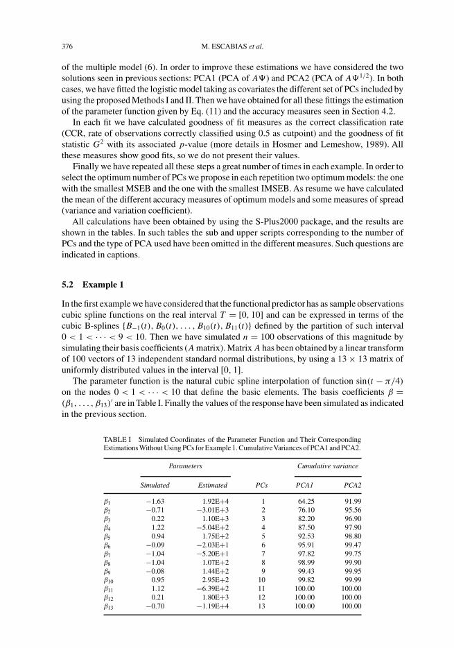
TABLE I Simulated Coordinates of the Parameter Function and Their CorrespondingEstimationsWithout Using PCs for Example 1. CumulativeVariances of PCA1 and PCA2.

Parameters Cumulative variance

Simulated Estimated PCs PCA1 PCA2

β1 −1.63 1.92E+4 1 64.25 91.99β2 −0.71 −3.01E+3 2 76.10 95.56β3 0.22 1.10E+3 3 82.20 96.90β4 1.22 −5.04E+2 4 87.50 97.90β5 0.94 1.75E+2 5 92.53 98.80β6 −0.09 −2.03E+1 6 95.91 99.47β7 −1.04 −5.20E+1 7 97.82 99.75β8 −1.04 1.07E+2 8 98.99 99.90β9 −0.08 1.44E+2 9 99.43 99.95β10 0.95 2.95E+2 10 99.82 99.99β11 1.12 −6.39E+2 11 100.00 100.00β12 0.21 1.80E+3 12 100.00 100.00β13 −0.70 −1.19E+4 13 100.00 100.00


FIGURE 1 Graphic of the simulated parameter function ( ) and its estimation (− − − −) without using PCs.

The estimation of the basis coefficients of the parameter function obtained without usingPCs is given in Table I and as we can see they are very different to the simulated ones dueto the great multicollinearity that exists in the approximated design matrix (1|A�). Figure 1shows the great difference between the simulated and estimated parameter functions. In spiteof this bad estimation, the model fits well with CCR of 90%, G2 = 44.8 and p-value = 1.00.The importance of obtaining a good estimation of the parameter function led us to improve itby using FPCA as proposed in previous section.

First, we have obtained the matrices �(1) and �(2) of PCs of the A� and A�1/2 matrices,respectively. These PCA1 and PCA2 approaches provide the explained variances given inTable I. Let us observe that the first five PCs explain more than 90% of the total variability andwith the first eight we reach nearly 99% in PCA1. However in PCA2 more than 91% of totalvariability is explained with only one PC, and nearly 99% with the first five.

Now, we have fitted the multiple models with a different number of PCs by including themin the model according to the different methods seen in previous sections: Methods I and II.The results of the different measures of accuracy of estimations can be seen in Table II forMethod I and Table III for Method II.

Let us observe from Table II the great increase of all measures obtained when we includethe last PCs in the model, which shows the need of choosing a smaller number of PCs in orderto obtain a good estimation of the parameter function. In addition all models fit well with CCRnext to 90% in most cases and p-value of G2 nearly 1.00.

We can see that in PCA1 the minimum values of IMSEB and MSEB are the ones corres-ponding to the model which has the first four PCs included by Method I (Tab. II) and themodel with the first, third and fourth PCs included by Method II (Tab. III). Then these modelsprovide the best possible estimations using this type of PCs with similar values of the accuracymeasures. This is not the case in PCA2, which by using Method I (Tab. II) IMSEB indicates thatthe best estimation is the one obtained with the model that includes the first five PCs, whereasMSEB indicates that the best model is the one with only the first PC. Method II (Tab. III)shows again this difference between MSEB and IMSEB for PCA2, being the optimum modelsthose with two PCs (first and fifth) and three (first, fifth and third) respectively. The estimatedparameter functions given by these optimum models can be seen in Figure 2(a), (b) and (c). Let


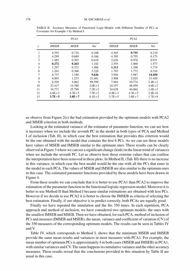
TABLE II Accuracy Measures of Functional Logit Models with Different Number of PCs asCovariates for Example 1 by Method I.

PCA1 PCA2

s IMSEB MSEB Var IMSEB MSEB Var

1 4.555 0.710 0.108 4.565 0.755 0.1102 4.299 0.689 0.166 4.395 0.755 0.1733 1.485 0.393 0.618 2.626 0.976 0.9314 0.272 0.263 1.242 2.555 1.060 1.5775 1.297 0.373 1.986 1.313 1.298 3.7746 1.263 0.368 3.228 1.793 1.772 6.2167 4.737 1.189 9.626 3.956 1.987 14.4508 4.895 1.233 21.481 3.908 2.025 31.4509 8.526 5.062 89.599 7.964 10.774 2.4E+2

10 23.417 14.780 2.0E+2 24.357 48.959 4.6E+211 34.771 35.790 7.2E+2 34.628 46.064 1.4E+312 4.4E+3 4.3E+5 7.5E+2 4.4E+3 4.3E+5 2.4E+613 3.7E+5 3.8E+7 8.1E+2 3.7E+5 3.8E+7 1.7E+8

us observe from Figure 2(c) the bad estimation provided by the optimum models with PCA2and MSEB criterion in both methods.

Looking at the estimated variance of the estimator of parameter function, we can see howit increases when we include the seventh PC in the model in both types of PCA and MethodI of inclusion (Tab. II), in which case the best estimation that provides this criterion wouldbe the one obtained with the model that contains the first 6 PCs. As we can see these modelshave values of MSEB and IMSEB similar to the optimum ones. These results can be clearlyobserved in Figure 3 where we can see a significant change (kink) in the linear trend of varianceswhen we include the seventh PC. Let us observe how those extreme values that can confusethe interpretation have been removed in these plots. In Method II, (Tab. III) there is no increasein this variance, in which case the best model would be the one with all the PCs that enter inthe model in each PCA. The values of MSEB and IMSEB are also similar to the optimum onesin this case. The estimated parameter functions provided by these models have been drawn inFigure 4.

From these results we can conclude that it is better to use PCA1 than PCA2 to improve theestimation of the parameter function in the functional logistic regression model. Moreover it isbetter to use Method II than Method I because similar estimations are obtained with less PCs.However if we decide to use PCA2 it is better to choose the IMSEB as criteria of selecting thebest estimation. Finally, if our objective is to predict correctly, both PCAs are equally good.

Finally we have repeated the simulation and the fits 350 times. In each repetition, PCAapproach and method of inclusion, we have considered two optimum models: the ones withthe smallest IMSEB and MSEB. Then we have obtained, for each PCA, method of inclusion ofPCs and measure (IMSEB and MSEB), the mean, variance and coefficient of variation (CV) ofthe 350 measures of the corresponding optimum models. The results can be seen in Tables IVand V.

Table IV, which corresponds to Method I, shows that the minimum MSEB and IMSEBprovide the same mean results and variances in most measures with PCA1. For example, themean number of optimum PCs is approximately 4 in both cases (MSEB and IMSEB) in PCA1,with similar variances and CV. The same happens in cumulative variance and the other accuracymeasures. These results reveal that the conclusions provided in this situation by Table II areusual in this case.


FIGURE 2 Example 1 – Graphics of the simulated parameter function ( ) and its estimation with Method I(− − − −) and Method II ( . . . . .): (a) PCA1: 4 PCs in Method I and 3 in Method II (MSEB and IMSEB criteria),(b) PCA2: 5 PCs in Method I and 3 in Method II (IMSE criterion), (c) PCA2: 1 PC in Method I and 2 in Method II(MSEB criterion). Graphics of the simulated parameter function ( ) and mean of its estimations with Method I(− − − −) and Method II ( . . . . . ) after 350 repetitions: (d) PCA1 and MSEB criterion, (e) PCA2 and IMSEB criterion,(f) PCA2 and MSEB criterion.

TABLE III Accuracy Measures of Functional Logit Models with Different Number of PCs as Covariates for Example1 by Method II.

PCA1 PCA2

s PCs IMSEB MSEB Var PCs IMSEB MSEB Var

1 1 4.555 0.710 0.108 1 4.565 0.755 0.1102 3 1.848 0.422 0.521 5 2.968 0.697 0.9803 4 0.564 0.288 1.137 3 1.544 1.236 2.858


FIGURE 3 Example 1 – Graphics of the estimated variance of the parameters with Method I after removing extremevalues: (a) PCA1, (b) PCA2.

In relation to PCA2 with Method I, the conclusions are the same as the ones we saw in thesingle simulation, now IMSEB and MSEB do not provide the same mean of optimum numberof PCs (Tab. IV). Furthermore the mean number of PCs that provides IMSEB is similar to theone obtained with PCA1.

In Table V (Method II) the conclusions are the same as the ones presented for Table IV,in relation to the convenience of using the minimum IMSEB or MSEB for selecting the bestestimation in PCA2. Moreover we can once again see a bigger reduction in the dimension ofthe problem than the one obtained in Table IV because the mean number of PCs needed issmaller than the one associated to Method I.

Finally we have calculated the mean of the optimum estimations of the parameter functionfor the optimum models provided by each type of PCA, method and criterion for selecting PCs(Fig. 2(d)–(f)). Let us observe again that PCA1 and Method II provide the best estimations.

5.3 Example 2

In the second example we have considered a different method of simulating the explicativesample paths. We have simulated observations of a set of 100 curves of a known stochasticprocess at the set of 21 equally spaced times of the [0, 10] interval (it is not necessary totake equally spaced times). More precisely we have considered the process used by Fraimanand Muniz (2001) X (t) = Z(t)+ t/4 + 5E where Z(t) is a zero mean Gaussian stochastic

FIGURE 4 Example 1 – Graphics of the simulated parameter function ( ) and its estimation given by Method I(− − − −) and Method II ( . . . . .) with variance criterion: (a) PCA1: 6 PCs in Method I and 3 in Method II, (b) PCA2:6 PCs in Method I and 3 in Method II.


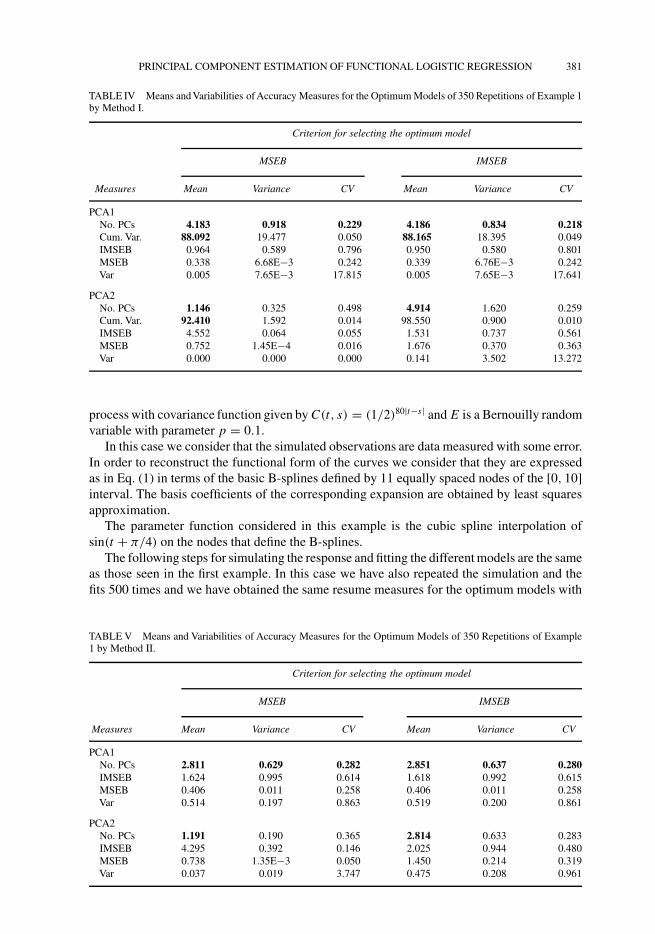
TABLE IV Means and Variabilities of Accuracy Measures for the Optimum Models of 350 Repetitions of Example 1by Method I.

Criterion for selecting the optimum model

MSEB IMSEB

Measures Mean Variance CV Mean Variance CV

PCA1No. PCs 4.183 0.918 0.229 4.186 0.834 0.218Cum. Var. 88.092 19.477 0.050 88.165 18.395 0.049IMSEB 0.964 0.589 0.796 0.950 0.580 0.801MSEB 0.338 6.68E−3 0.242 0.339 6.76E−3 0.242Var 0.005 7.65E−3 17.815 0.005 7.65E−3 17.641

PCA2No. PCs 1.146 0.325 0.498 4.914 1.620 0.259Cum. Var. 92.410 1.592 0.014 98.550 0.900 0.010IMSEB 4.552 0.064 0.055 1.531 0.737 0.561MSEB 0.752 1.45E−4 0.016 1.676 0.370 0.363Var 0.000 0.000 0.000 0.141 3.502 13.272

process with covariance function given by C(t, s) = (1/2)80|t−s| and E is a Bernouilly randomvariable with parameter p = 0.1.

In this case we consider that the simulated observations are data measured with some error.In order to reconstruct the functional form of the curves we consider that they are expressedas in Eq. (1) in terms of the basic B-splines defined by 11 equally spaced nodes of the [0, 10]interval. The basis coefficients of the corresponding expansion are obtained by least squaresapproximation.

The parameter function considered in this example is the cubic spline interpolation ofsin(t + π/4) on the nodes that define the B-splines.

The following steps for simulating the response and fitting the different models are the sameas those seen in the first example. In this case we have also repeated the simulation and thefits 500 times and we have obtained the same resume measures for the optimum models with

TABLE V Means and Variabilities of Accuracy Measures for the Optimum Models of 350 Repetitions of Example1 by Method II.


MSEB IMSEB


PCA1No. PCs 2.811 0.629 0.282 2.851 0.637 0.280IMSEB 1.624 0.995 0.614 1.618 0.992 0.615MSEB 0.406 0.011 0.258 0.406 0.011 0.258Var 0.514 0.197 0.863 0.519 0.200 0.861

PCA2No. PCs 1.191 0.190 0.365 2.814 0.633 0.283IMSEB 4.295 0.392 0.146 2.025 0.944 0.480MSEB 0.738 1.35E−3 0.050 1.450 0.214 0.319Var 0.037 0.019 3.747 0.475 0.208 0.961


FIGURE 5 Graphics of the simulated parameter function ( ) and the mean of its estimations with Method I(− − − −) and Method II ( . . . . . ) after 500 repetitions of Example 2: (a) PCA1 and MSEB criterion, (b) PCA1 andIMSEB criterion, (c) PCA2 and MSEB criterion, (d) PCA2 and IMSEB criterion.

each PCA, method and criterion for choosing the PCs. The results are presented in Tables VIfor Method I and Table VII for Method II. From such tables we can see again the great reduc-tion of dimension that provides the best possible estimation of the parameter function. Onthe one hand, by using PCA1, we can see the great reduction of dimension obtained with amean number of PCs in the optimum estimation rounding the three and four (Method II and

TABLE VI Means and Variabilities of Accuracy Measures for the Optimum Models of 500 Repetitions of Example2 by Method I.


MSEB IMSEB


PCA1No. PCs 4.592 2.622 0.353 4.496 1.100 0.233Cum Var. 78.305 78.563 0.113 78.550 27.614 0.067IMSEB 1.140 1.310 1.004 0.907 0.489 0.771MSEB 0.411 0.058 0.585 0.446 0.113 0.754Var 0.001 3.16E−7 0.978 0.001 1.09E−7 0.650

PCA2No. PCs 1.340 1.676 0.966 7.472 6.903 0.352Cum Var. 79.443 11.110 0.042 93.810 22.026 0.050IMSEB 4.778 0.533 0.153 1.743 0.329 0.329MSEB 0.854 0.016 0.150 11.658 138.080 1.008Var 0.002 3.92E−4 10.607 0.048 8.41E−3 1.897


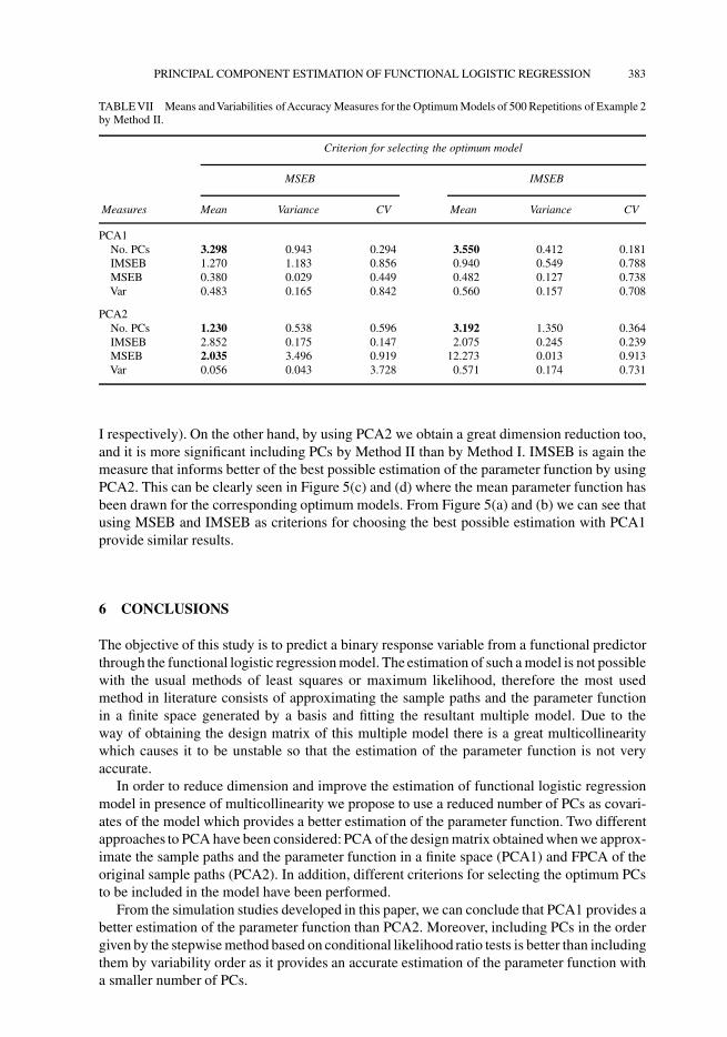
TABLE VII Means andVariabilities ofAccuracy Measures for the Optimum Models of 500 Repetitions of Example 2by Method II.


MSEB IMSEB




I respectively). On the other hand, by using PCA2 we obtain a great dimension reduction too,and it is more significant including PCs by Method II than by Method I. IMSEB is again themeasure that informs better of the best possible estimation of the parameter function by usingPCA2. This can be clearly seen in Figure 5(c) and (d) where the mean parameter function hasbeen drawn for the corresponding optimum models. From Figure 5(a) and (b) we can see thatusing MSEB and IMSEB as criterions for choosing the best possible estimation with PCA1provide similar results.

6 CONCLUSIONS

The objective of this study is to predict a binary response variable from a functional predictorthrough the functional logistic regression model. The estimation of such a model is not possiblewith the usual methods of least squares or maximum likelihood, therefore the most usedmethod in literature consists of approximating the sample paths and the parameter functionin a finite space generated by a basis and fitting the resultant multiple model. Due to theway of obtaining the design matrix of this multiple model there is a great multicollinearitywhich causes it to be unstable so that the estimation of the parameter function is not veryaccurate.

In order to reduce dimension and improve the estimation of functional logistic regressionmodel in presence of multicollinearity we propose to use a reduced number of PCs as covari-ates of the model which provides a better estimation of the parameter function. Two differentapproaches to PCA have been considered: PCA of the design matrix obtained when we approx-imate the sample paths and the parameter function in a finite space (PCA1) and FPCA of theoriginal sample paths (PCA2). In addition, different criterions for selecting the optimum PCsto be included in the model have been performed.

From the simulation studies developed in this paper, we can conclude that PCA1 provides abetter estimation of the parameter function than PCA2. Moreover, including PCs in the ordergiven by the stepwise method based on conditional likelihood ratio tests is better than includingthem by variability order as it provides an accurate estimation of the parameter function witha smaller number of PCs.


Acknowledgements

This research has been funded by BFM2000-1466 project from the Spanish Ministry ofScience and Technology. The authors thanks an anonymous referee for helpful commentsand suggestions that have contributed to improve the final version of this paper.

References

Aguilera, A. M. and Escabias, M. (2000). Principal component logistic regression. Proceedings in ComputationalStatistics 2000, Physica-Verlag, pp. 175–180.Aguilera, A. M., Gutierrez, R., Ocana, F. A. and Valderrama, M. J. (1995). Computational approaches to estimation

in the principal component analysis of a stochastic process. Applied Stochastic Models and Data Analysis, 11(4),279–299.

Aguilera, A. M., Gutierrez, R. and Valderrama, M. J. (1996). Approximation of estimators in the PCA of a stochasticprocess using B-splines. Communications in Statistics: Computation and Simulation, 25(3), 671–690.

Aguilera, A. M., Ocana, F. A. and Valderrama, M. J. (1997a). An approximated principal component prediction modelfor continuous-time stochastic processes. Applied Stochastic Models and Data Analysis, 13(1), 61–72.

Aguilera, A. M., Ocana, F. A. and Valderrama, M. J. (1997b). Regresion sobre componentes principales de un procesoestocastico con funciones muestrales escalonadas. Estadistica Espanola, 39(142), 5–21.

Aguilera, A. M., Ocana, F. A. and Valderrama, M. J. (1999a). Forecasting time series by functional PCA. Discussionof several weighted approaches. Computational Statistics, 14, 442–467.

Aguilera, A. M., Ocana, F. A. and Valderrama, M. J. (1999b). Forecasting with unequally spaced data by a functionalprincipal component approach. Test, 8(1), 233–253.

Aguilera, A. M., Ocana, F. A. and Valderrama, M. J. (2002). Estimating functional principal component analysis onfinite-dimensional data spaces. Computational Statistics and Data Analysis (Submitted).

Aucott, L. S., Garthwaite, P. H. and Currall, J. (2000). Regression methods for high dimensional multicollinear data.Communications in Statistics: Computation and Simulation, 29(4), 1021–1037.

De Boor, C. (1978). A Practical Guide to Splines, Springer-Verlag.Fraiman, R. and Muniz, G. (2001). Trimmed means for functional data. Test, 10(2), 419–440.Hocking, R. R. (1976). The analysis and selection of variables in linear regression. Biometrics, 32, 1–49.Hosmer, D. W. and Lemeshow, S. (1989). Applied Logistic Regression, Wiley.Jackson, J. E. (1991). An User’s Guide to Principal Components, Wiley.James, G. M. (2002). Generalized linear models with functional predictors. Journal of the Royal Statistical Society,

Series B, 64(3), 411–432.Liang, K-Y. and Zeger, S. L. (1986). Longitudinal data analysis using generalized linear models. Biometrika, 73(1),

13–22.Muller, H-G. and Stadmuller, U. (2002). Generalized functional linear models. Unpublished paper.McCullagh, P. and Nelder, J. A. (1983). Generalized Linear Models, Chapman & Hall.Ramsay, J. O. and Silverman, B. W. (1997). Functional Data Analysis, Springer-Verlag.Ramsay, J. O. and Silverman, B. W. (2002). Applied Functional Data Analysis, Springer-Verlag.Ratcliffe, S. J., Heller, G. Z. and Leader, L. R. (2002). Functional data analysis with application to periodically

stimulated foetal heart rate data. II: Functional logistic regression. Statistics in Medicine, 21, 1115–1127.Ryan, T. P. (1997). Modern Regression Methods, Wiley.Todorovic, P. (1992). An Introduction to Stochastic Processes and their Applications, Springer-Verlag.Valderrama, M. J., Aguilera, A. M. and Ocana, F. A. (2000). Prediccion Dinamica Mediante Analisis de Datos

Funcionales, Hesperides-La Muralla.Valderrama, M. J., Ocana, F. A. and Aguilera, A. M. (2002). Forecasting PC-ARIMA models for functional data.

Proceedings in Computational Statistics, Physica-Verlag, pp. 25–36.

principal component estimation of …hera.ugr.es/doi/15057823.pdfprincipal component estimation of...

Documents