principal arc analysis on direct product manifolds · principal arc analysis on direct product ......

The Annals of Applied Statistics2011, Vol. 5, No. 1, 578–603DOI: 10.1214/10-AOAS370© Institute of Mathematical Statistics, 2011

PRINCIPAL ARC ANALYSIS ON DIRECT PRODUCT MANIFOLDS

BY SUNGKYU JUNG, MARK FOSKEY AND J. S. MARRON

University of North Carolina, University of North Carolina andUniversity of North Carolina

We propose a new approach to analyze data that naturally lie on mani-folds. We focus on a special class of manifolds, called direct product man-ifolds, whose intrinsic dimension could be very high. Our method finds alow-dimensional representation of the manifold that can be used to find andvisualize the principal modes of variation of the data, as Principal ComponentAnalysis (PCA) does in linear spaces. The proposed method improves uponearlier manifold extensions of PCA by more concisely capturing importantnonlinear modes. For the special case of data on a sphere, variation followingnongeodesic arcs is captured in a single mode, compared to the two modesneeded by previous methods. Several computational and statistical challengesare resolved. The development on spheres forms the basis of principal arcanalysis on more complicated manifolds. The benefits of the method are il-lustrated by a data example using medial representations in image analysis.

1. Introduction. Principal Component Analysis (PCA) has been frequentlyused as a method of dimension reduction and data visualization for high-dimensional data. For data that naturally lie in a curved manifold, application ofPCA is not straightforward since the sample space is not linear. Nevertheless, theneed for PCA-like methods is growing as more manifold data sets are encounteredand as the dimensions of the manifolds increase.

In this article we introduce a new approach for an extension of PCA on a spe-cial class of manifold data. We focus on direct products of simple manifolds, inparticular, of the unit circle S1, the unit sphere S2, R+ and R

p . We will referto these as direct product manifolds, for convenience. Many types of statisticalsample spaces are special cases of the direct product manifold. A widely knownexample is the sample space for directional data [Fisher (1993), Fisher, Lewis andEmbleton (1993) and Mardia and Jupp (2000)] and their direct products. Appli-cations include analysis of wind directions, orientations of cracks, magnetic fielddirections and directions from the earth to celestial objects. For example, when weconsider multiple 3-D directions simultaneously, the sample space is S2 ⊗· · ·⊗S2,which is a direct product manifold. Another example is the medial representationof shapes [m-reps, Siddiqi and Pizer (2008)], which is somewhat less known tothe statistical community but provides a powerful parametrization of 3-D shapes

Received December 2009; revised May 2010.Key words and phrases. Principal Component Analysis, nonlinear dimension reduction, mani-

fold, folded Normal distribution, directional data, image analysis, medial representation.

578

http://www.imstat.org/aoas/

http://dx.doi.org/10.1214/10-AOAS370

http://www.imstat.org

PRINCIPAL ARC ANALYSIS 579

of human organs and has been extensively studied in the image analysis field.The space of m-reps is usually a high-dimensional direct product manifold. Somebackground and necessary definitions on direct product manifolds can be found inAppendix.

Our approach to a manifold version of PCA builds upon earlier work, espe-cially the principal geodesic analysis proposed by Fletcher et al. (2004) and thegeodesic PCA proposed by Huckemann and Ziezold (2006) and Huckemann, Hotzand Munk (2010). A detailed catalogue of current methodologies can be found inHuckemann, Hotz and Munk (2010). An important approach among these is toapproximate the manifold by a linear space. Fletcher et al. (2004) take the tangentspace of the manifold at the geodesic mean as the linear space, and work withappropriate mappings between the manifold and the tangent space. This results infinding the best fitting geodesics among those passing through the geodesic mean.This was improved in an important way by Huckemann, Hotz and Munk, whofound the best fit over the set of all geodesics. Huckemann, Hotz and Munk wenton to propose a new notion of center point, the PCmean, which is an intersectionof the first two principal geodesics. This approach gives significant advantages, es-pecially when the curvature of the manifold makes the geodesic mean inadequate,an example of which is depicted in Figure 2b.

Our method inherits advantages of these methods and improves further by ef-fectively capturing more complex nongeodesic modes of variation. Note that thecurvature of direct product manifolds is mainly due to the spherical part, whichmotivates careful investigation of S2-valued variables. We point out that (small)circles in S2, including geodesics, can be used to capture the nongeodesic varia-tion. We introduce the principal circles and principal circle mean, analogous to,yet more flexible than, the geodesic principal component and PCmean of Hucke-mann, Hotz and Munk. These become principal arcs when the manifold is indeedS2. For more complex direct product manifolds, we suggest transforming the datapoints in S2 into a linear space by a special mapping utilizing the principal cir-cles. For the other components of the manifold, the tangent space mappings canbe used to map the data into a linear space as done in Fletcher et al. (2004). Oncemanifold-valued data are mapped onto the linear space, then the classical linearPCA can be applied to find principal components in the transformed linear space.The estimated principal components in the linear space can be back-transformedto the manifold, which leads to principal arcs.

We illustrate the potential of our method by an example of m-rep data in Fig-ure 1. Here, m-reps with 15 sample points called atoms model the prostate gland(an organ in the male reproductive system) and come from the simulator developedand analyzed in Jeong et al. (2008). Figure 1 shows that the S2 components of thedata tend to be distributed along small circles, which frequently are not geodesics.We emphasize the curvature of variation along each sphere by fitting a great circleand a small circle (by the method discussed in Section 2). Our method is adapted

580 S. JUNG, M. FOSKEY AND J. S. MARRON

FIG. 1. S2-valued samples (n = 60) of the prostate m-reps with 15 medial atoms. One sample inthis figure is represented by a 30-tuple of 3-D directions (two directions at each atom), which lies inthe manifold

⊗15i=1(S2 ⊗ S2). Small and great circles are fitted and plotted in the rightmost atoms

to emphasize the sample variation along small circles.

to capture this nonlinear (nongeodesic) variation of the data. A potential applica-tion of our method is to improve accuracy of segmentation of objects from CTimages. Detailed description of the data and results of our analysis can be found inSection 5.

Note that the previous approaches [Fletcher et al. (2004), Huckemann andZiezold (2006)] are defined for general manifolds, while our method focuses onthese particular direct product manifolds. Although the method is not applicablefor general manifolds, it is useful for this common class of manifolds that is oftenfound in applications. Our results inform our belief that focusing on specific typesof manifolds allow more precise and informative statistical modeling than methodsthat attempt to be fully universal. This happens through using special properties(e.g., presence of small circles) that are not available for all other manifolds.

The rest of the article is organized as follows. We begin by introducing a circleclass on S2 as an alternative to the set of geodesics. Section 2 discusses principalcircles in S2, which will be the basis of the special transformation. The first prin-cipal circle is defined by the least-squares circle, minimizing the sum of squaredresiduals. In Section 3 we introduce a data-driven method to decide whether theleast-squares circle is appropriate. A recipe for principal arc analysis on directproduct manifolds is proposed in Section 4 with discussion on the transforma-tions. A detailed introduction of the space of m-reps and the results from applyingthe proposed method follow. A novel computational algorithm for the least-squarescircles is presented in Section 6. In the Appendix we provide some necessary back-ground for treating direct product manifolds as sample spaces, including the notionof geodesic mean, tangent space, exponential map and log map.


2. Circle class for nongeodesic variation on S2. Consider a set of pointsin R

2. Numerous methods for understanding population properties of a data setin linear space have been proposed and successfully applied, which include rigidmethods, such as linear regression and principal components, and very flexiblemethods, such as scatterplot smoothing and principal curves [Hastie and Stuet-zle (1989)]. In this paper we make use of a parametric class of circles, includingsmall and great circles, which allows much more flexibility than either methods ofFletcher et al. (2004) or Huckemann, Hotz and Munk (2010), but less flexibilitythan a principal curve approach. Although this idea was motivated by examplessuch as those in Figure 1, there are more advantages gained from using the classof circles:

(i) The circle class includes the simple geodesic case.(ii) Each circle can be parameterized, which leads to an easy interpretation.

(iii) There is an orthogonal complement of each circle, which gives two importantadvantages:(a) Two orthogonal circles can be used as a basis of a further extension to

principal arc analysis.(b) Building a sensible notion of principal components on S2 alone is easily

done by utilizing the circles.

The idea (iii)(b) will be discussed in detail after introducing a method of circlefitting. Some notations follow: S2 can be thought of as the unit sphere in R

3, sothat a unit vector x ∈ R

3 is a member of S2. The geodesic distance between x,y ∈S2, denoted by ρ(x,y), is defined as the shortest distance between x, y along thesphere, which is the same as the angle formed by the two vectors. Thus, ρ(x,y) =cos−1(x′y). A circle on S2 is conveniently parameterized by center c ∈ S2 andgeodesic radius r , and denoted by δ(c, r) = {x ∈ S2|ρ(c,x) = r}. It is a geodesicwhen r = π/2. Otherwise it is a small circle.

A circle that best fits the points x1, . . . ,xn ∈ S2 is found by minimizing the sumof squared residuals. The residual of xi is defined as the signed geodesic distancefrom xi to the circle δ(c, r). Then the least-squares circle is obtained by

minc,r

n∑i=1

(ρ(xi , c) − r

)2 subject to c ∈ S2, r ∈ (0, π).(1)

Note that there are always multiple solutions of (1). In particular, whenever (c, r)is a solution, (−c, π − r) also solves the problem as δ(c, r) = δ(−c, π − r). Thisambiguity does not affect any essential result in this paper. Our convention is touse the circle with smaller geodesic radius.

The optimization task (1) is a constrained nonlinear least squares problem. Wepropose an algorithm to solve the problem that features a simplified optimizationtask and approximation of S2 by tangent planes. The algorithm works in a dou-bly iterative fashion, which has been shown by experience to be stable and fast.Section 6 contains a detailed illustration of the algorithm.


Analogous to principal geodesics in S2, we can define principal circles in S2 byutilizing the least-squares circle. The principal circles are two orthogonal circlesin S2 that best fit the data. We require the first principal circle to minimize thevariance of the residuals, so it is the least-squares circle (1). The second principalcircle is a geodesic which passes through the center of the first circle and thus isorthogonal at the points of intersection. Moreover, the second principal circle ischosen so that one intersection point is the intrinsic mean [defined in (2) later] ofthe projections of the data onto the first principal circle.

Based on a belief that the intrinsic (or extrinsic) mean defined on a curvedmanifold may not be a useful notion of the center point of the data [see, e.g.,Huckemann, Hotz and Munk and Figure 2b], the principal circles do not use thepre-determined means. To develop a better notion of center point, we locate thebest 0-dimensional representation of the data in a data-driven manner. Inspired bythe PCmean idea of Huckemann, Hotz and Munk, given the first principal circleδ1, the principal circle mean u ∈ δ1 is defined (in an intrinsic way) as

u = argminu∈δ1

n∑i=1

ρ2(u,Pδ1xi ),(2)

where Pδ1x is the projection of x onto δ1, that is, the point on δ1 of the shortestgeodesic distance to x. Then

Pδ1(c,r)x = x sin(r) + c sin(ρ(x, c) − r)

sin(ρ(x, c)),(3)

as in equation (3.3) of Mardia and Gadsden (1977). We assume that c is the northpole e3, without losing generality since otherwise the sphere can be rotated. Then

ρ(u,Pδ1x) = sin(r)ρS1

((u1, u2)√

1 − u23

,(x1, x2)√

1 − x23

),(4)

where u = (u1, u2, u3)′, x = (x1, x2, x3)

′ and ρS1 is the geodesic (angular) distancefunction on S1. The optimization problem (2) is equivalent to finding the geodesicmean in S1. See equation (17) in the Appendix for computation of the geodesicmean in S1.

The second principal circle δ2 is then the geodesic passing through the principalcircle mean u and the center c of δ1. Denote δ ≡ δ(x1, . . . ,xn) as a combinedrepresentation of (δ1,u) or, equivalently, (δ1, δ2).

As a special case, we can force the principal circles to be great circles. Thebest fitting geodesic is obtained as a solution of the problem (1) with r = π/2and becomes the first principal circle. The optimization algorithm for this caseis slightly modified from the original algorithm for the varying r case by simplysetting r = π/2. The principal circle mean u and the δ2 for this case are definedin the same way as in the small circle case. Note that the principal circles withr = π/2 are essentially the same as the method of Huckemann and Ziezold (2006).


(a) (b)

(c) (d)

FIG. 2. Toy examples on S2 with n = 30 points showing the first principal circle (red) as a smallcircle and the first geodesic principal component (dotted green) by Huckemann, and the first princi-pal geodesic (black) by Fletcher. Also plotted are the geodesic mean, PCmean and principal circlemean of the data as black, green and red diamonds, respectively. (a) The three methods give similarsatisfactory answers when the data are stretched along a geodesic. (b) When the data are stretchedalong a great circle, covering almost all of it, the principal geodesic (black circle) and geodesic mean(black diamond) fail to find a reasonable representation of the data, while the principal circle andHuckemann’s geodesic give sensible answers. (c) Only the principal circle fits well when the dataare not along a geodesic. (d) For a small cluster without principal modes of variation, the principalcircle gets too small. See Section 3 for discussion of this phenomenon.

Figure 2 illustrates the advantages of using the circle class to efficiently sum-marize variation. On four different sets of toy data, the first principal circle δ1 isplotted with principal circle mean u. The first principal geodesics from the methodsof Fletcher and Huckemann are also plotted with their corresponding mean. Fig-ure 2a illustrates the case where the data were indeed stretched along a geodesic.The solutions from the three methods are similar to one another. The advantageof Huckemann’s method over Fletcher’s can be found in Figure 2b. The geodesicmean is found far from the data, which leads to poor performance of the principalgeodesic analysis, because it considers only great circles passing through the geo-


desic mean. Meanwhile, the principal circle and Huckemann’s method, which donot utilize the geodesic mean, work well. The case where geodesic mean and anygeodesic do not fit the data well is illustrated in Figure 2c, which is analogous tothe Euclidean case, where a nonlinear fitting may do a better job of capturing thevariation than PCA. To this data set, the principal circle fits best, and our defini-tion of mean is more sensible than the geodesic mean and the PCmean. The pointsin Figure 2d are generated from the von Mises–Fisher distribution with κ = 10,thus having no principal mode of variation. In this case the first principal circleδ1 follows a contour of the apparent density of the points. We shall discuss thisphenomenon in detail in the following section.

Fitting a (small) circle to data on a sphere has been investigated for some time,especially in statistical applications in geology. Those approaches can be distin-guished in three different ways, where our choice fits into the first category:

(1) Least-squares of intrinsic residuals: Gray, Geiser and Geiser (1980) formulatedthe same problem as in (1), finding a circle that minimizes sum of squaredresiduals, where residuals are defined in a geodesic sense.

(2) Least-squares of extrinsic residuals: A different measure of residual was cho-sen by Mardia and Gadsden (1977) and Rivest (1999), where the residual ofx from δ(c, r) is defined by the shortest Euclidean distance between x andδ(c, r). Their objective is to find

argminδ

n∑i=1

‖xi − Pδxi‖2 = argminδ

n∑i=1

−x′iPδxi = argmin

δ

n∑i=1

− cos(ξi),

where ξi denotes the intrinsic residual. This type of approach can be numeri-cally close to the intrinsic method as cos(ξi) = 1 − ξ2

i /2 + O(ξ4i ).

(3) Distributional approach: Mardia and Gadsden (1977) and Bingham and Mar-dia (1978) proposed appropriate distributions to model S2-valued data thatcluster near a small circle. These models essentially depend on the quantitycos(ξ), which is easily interpreted in the extrinsic sense but not in the intrinsicsense.

REMARK. The principal circle and principal circle mean always exist. This isbecause the objective function (1) is a continuous function of c, with the compactdomain S2. The minimizer r has a closed-form solution (see Section 6). A similarargument can be made for the existence of u. On the other hand, the uniqueness ofthe solution is not guaranteed. We conjecture that if the manifold is approximatelylinear or, equivalently, the data set is well approximated by a linear space, then theprincipal circle will be unique. However, this does not lead to the uniqueness of u,whose sufficient condition is that the projected data on δ1 is strictly contained in ahalf-circle [Karcher (1977)]. Note that a sufficient condition for the uniqueness ofthe principal circle is not clear even in the Euclidean case [Chernov (2010)].


3. Suppressing small least-squares circles. When the first principal circle δ1has a small radius, sometimes it is observed that δ1 does not fit the data in a mannerthat gives useful decomposition, as shown in Figure 2d. This phenomenon has beenalso observed for the related principal curve fitting method of Hastie and Stuetzle(1989). We view this as unwanted overfitting, which is indeed a side effect causedby using the full class of circles with free radius parameter instead a class of greatcircles. In this section a data-driven method to flag this overfitting is discussed. Inessence, the fitted small circle is replaced by the best fitting geodesics when thedata do not cluster along the circle but instead tend to cluster near the center of thecircle.

We first formulate the problem and solution in R2. This is for the sake of clear

presentation and also because the result on R2 can be easily extended to S2 using

a tangent plane approximation.Let fX be a spherically symmetric density function of a continuous distribution

defined on R2. Whether the density is high along some circle is of interest. By the

symmetry assumption, density height along a circle can be found by inspectinga section of fX along a ray from the origin (the point of symmetry). A sectionof fX coincides with the conditional density fX1|X2(x1|x2 = 0) = κ−1fX(x1,0).A random variable corresponding to the p.d.f. fX1|X2=0 is not directly observable.Instead, the radial distance R = ‖X‖ from the origin can be observed. For the po-lar coordinates (R,�) such that X = (X1,X2) = (R cos�,R sin�), the marginalp.d.f. of R is fR(r) = 2πrfX(r,0) as fX is spherically symmetric. A section of fXis related to the observable density fR as fR(r) ∝ rfX1|X2=0(r), for r ≥ 0. Thisrelation is called the length-biased sampling problem [Cox (1969)]. The relationcan be understood intuitively by observing that a value r of R can be observed atany point on a circle of radius r , circumference of which is proportional to r . Thus,sampling of R from the density fX1|X2=0 is proportional to its size.

The problem of suppressing a small circle can be paraphrased as “how to deter-mine whether a nonzero point is a mode of the function fX1|X2=0, when observingonly a length-biased sample.”

The spectrum from the circle-clustered case (mode at a nonzero point) to thecenter-clustered case (mode at origin) can be modeled as

data = signal + error,(5)

where the signal is along a circle with radius μ, and the error accounts for theperpendicular deviation from the circle (see Figure 3). Then, in polar coordinates(R,�), � is uniformly distributed on (0,2π ] and R is a positive random variablewith mean μ. First assume that R follows a truncated Normal distribution withstandard deviation σ , with the marginal p.d.f. proportional to

fR(r) ∝ φ

(r − μ

σ

)for r ≥ 0,(6)


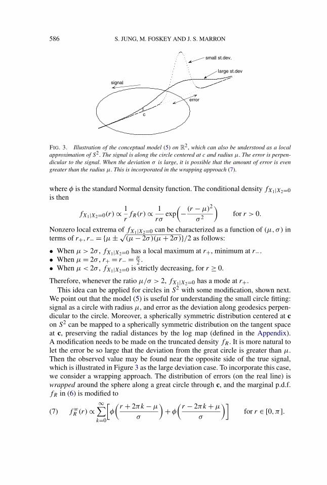
FIG. 3. Illustration of the conceptual model (5) on R2, which can also be understood as a local

approximation of S2. The signal is along the circle centered at c and radius μ. The error is perpen-dicular to the signal. When the deviation σ is large, it is possible that the amount of error is evengreater than the radius μ. This is incorporated in the wrapping approach (7).

where φ is the standard Normal density function. The conditional density fX1|X2=0is then

fX1|X2=0(r) ∝ 1

rfR(r) ∝ 1

rσexp

(−(r − μ)2

σ 2

)for r > 0.

Nonzero local extrema of fX1|X2=0 can be characterized as a function of (μ,σ ) interms of r+, r− = {μ ± √

(μ − 2σ)(μ + 2σ)}/2 as follows:

• When μ > 2σ , fX1|X2=0 has a local maximum at r+, minimum at r−.• When μ = 2σ , r+ = r− = μ

2 .

• When μ < 2σ , fX1|X2=0 is strictly decreasing, for r ≥ 0.

Therefore, whenever the ratio μ/σ > 2, fX1|X2=0 has a mode at r+.This idea can be applied for circles in S2 with some modification, shown next.

We point out that the model (5) is useful for understanding the small circle fitting:signal as a circle with radius μ, and error as the deviation along geodesics perpen-dicular to the circle. Moreover, a spherically symmetric distribution centered at con S2 can be mapped to a spherically symmetric distribution on the tangent spaceat c, preserving the radial distances by the log map (defined in the Appendix).A modification needs to be made on the truncated density fR . It is more natural tolet the error be so large that the deviation from the great circle is greater than μ.Then the observed value may be found near the opposite side of the true signal,which is illustrated in Figure 3 as the large deviation case. To incorporate this case,we consider a wrapping approach. The distribution of errors (on the real line) iswrapped around the sphere along a great circle through c, and the marginal p.d.f.fR in (6) is modified to

f wR (r) ∝

∞∑k=0

[φ

(r + 2πk − μ

σ

)+ φ

(r − 2πk + μ

σ

)]for r ∈ [0, π].(7)


FIG. 4. (Left) Graph of f wX1|X2=0(r) for μ/σ = 1,2,3,4. The density is high at a nonzero

point when μ/σ > 2.0534. (Center, right) Spherically symmetric distributions f corresponding toμ/σ = 2,3. The ratio μ/σ > 2 roughly leads to a high density along a circle.

The corresponding conditional p.d.f., f wX1|X2=0, is similar to fX1|X2=0 and a numer-

ical calculation shows that f wX1|X2=0 has a mode at some nonzero point whenever

μ/σ > 2.0534, for μ < π/2. In other words, we use the small circle when μ/σ islarge. Note that in what follows we only consider the first term (k = 0) of (7) sinceother terms are negligible in most situations. We have plotted f w

X1|X2=0 for someselected values of μ and σ in Figure 4.

With a data set on S2, we need to estimate μ and σ , or the ratio μ/σ . Letx1, . . . ,xn ∈ S2 and let c be the samples and the center of the fitted circle, respec-tively. Denote ξi for the errors of the model (5) such that ξi ∼ N(0, σ 2). Thenri ≡ ρ(xi , c) = |μ + ξi |, which has the folded normal distribution [Leone, Nel-son and Nottingham (1961)]. Estimation of μ and σ based on unsigned ri is notstraightforward. We present two different approaches to this problem.

Robust approach. The observations r1, . . . , rn can be thought of as a set of posi-tive numbers contaminated by the folded negative numbers. Therefore, the left half(near zero) of the data are more contaminated than the right half. We only use theright half of the data, which are less contaminated than the other half. We proposeto estimate μ and σ by

μ = med(rn1 ), σ = (

Q3(rn1 ) − med(rn

1 ))/Q3(),(8)

where Q3() is the third quantile of the standard normal distribution. The ratiocan be estimated by μ/σ .

Likelihood approach via EM algorithm. The problem may also be solved by alikelihood approach. Early solutions can be found in Leone, Nelson and Notting-ham (1961), Elandt (1961) and Johnson (1962), in which the MLEs were given bynumerically solving nonlinear equations based on the sample moments. As thosemethods were very complicated, we present a simpler approach based on the EMalgorithm. Consider unobserved binary variables si with values −1 and +1 so thatsiri ∼ N(μ,σ 2). The idea of the EM algorithm is that if we have observed si , then


the maximum likelihood estimator of ϑ = (μ,σ 2) would be easily obtained. TheEM algorithm is an iterative algorithm consisting of two steps. Suppose that thekth iteration produced an estimate ϑk of ϑ . The E-step is to impute si based on riand ϑk by forming a conditional expectation of log-likelihood for ϑ ,

Q(ϑ) = E

[log

n∏i=1

f (ri, si |ϑ)∣∣∣ri, ϑk

]

=n∑

i=1

[logf (ri |si = +1, ϑ)P (si = +1|ri, ϑk)

+ logf (ri |si = −1, ϑ)P (si = −1|ri, ϑk)]

=n∑

i=1

[logφ(ri |ϑ)pi(k) + logφ(−ri |ϑ)

(1 − pi(k)

)],

where f is understood as an appropriate density function, and pi(k) is easily com-puted as

pi(k) = P(si = +1|ri, ϑk) = φ(ri |ϑk)

φ(ri |ϑk) + φ(−ri |ϑk).

The M-step is to maximize Q(ϑ) whose solution becomes the next estimator ϑk+1.Now the (k + 1)th estimates are calculated by a simple differentiation and givenby

μk+1 = 1

n

n∑i=1

(2pi(k) − 1

)ri, σ 2

k+1 = 1

n

n∑i=1

(r2i − μ2

k+1).

With the sample mean and variance of r1, . . . , rn as an initial estimator ϑ0, thealgorithm iterates E-steps and M-steps until the iteration changes the estimatesless than a predefined criteria (e.g., 10−10). μ/σ is estimated by the ratio of thesolutions.

Comparison. Performance of these estimators are now examined by a simula-tion study. Normal random samples are generated with ratios μ/σ being 0, 1, 2or 3, representing the transition from the center-clustered to circle-clustered case.For each ratio, n = 50 samples are generated, from which μ/σ is estimated. Thesesteps are repeated 1000 times to obtain the sampling variation of the estimates.We also study the n = 1000 case in order to investigate the consistency of theestimators. The results are summarized in Figure 5 and Table 1.

The distribution of estimators are shown for n = 50,1000 in Figure 5 and theproportion of estimators greater than 2 is summarized in Table 1. When n = 1000,both estimators are good in terms of the proportion of correct answers. In the fol-lowing, the proportions of correct answers are corresponding to n = 50 case. The


FIG. 5. Simulation results of the proposed estimators for the ratio μ/σ . Different ratios repre-sent different underlying distributions. For example, estimators in the top left are based on randomsamples from a folded Normal distribution with mean μ = 3, standard deviation σ = 1. Curves aresmooth histograms of estimates from 1000 repetitions. The thick black curve represents the distribu-tion of the robust estimator from n = 50 samples. Likewise, the thick red curve is for the MLE withn = 50, the dotted black curve is for the robust estimator with n = 1000, and the dotted red curve isfor the MLE with n = 1000. The smaller sample size represents a usual data analytic situation, whilethe n = 1000 case shows an asymptotic situation.

top left panel in Figure 5 illustrates the circle-centered case with ratio 3. The esti-mated ratios from the robust approach give correct solutions (greater than 2) 95%of the time (98.5% for likelihood approach). For the borderline case (ratio 2, topright), the small circle will be used about half the time. The center-clustered caseis demonstrated with the true ratio 1, that also gives a reasonable answer (propor-tion of correct answers 95.3% and 94.8% for the robust and likelihood answersrespectively). It can be observed that when the true ratio is zero, the robust esti-mates are far from 0 (the bottom right in Figure 5). However, this is expected tooccur because the proportion of uncontaminated data is low when the ratio is toosmall. However, those ‘inaccurate’ estimates are around 1 and less than 2 most ofthe time, which leads to ‘correct’ answers. The likelihood approach looks some-what better with more hits near zero, but an asymptotic study [Johnson (1962)]


TABLE 1Proportion of estimates greater than 2 from the data illustrated in Figure 5. For μ/σ = 3, shown

are proportions of correct answers from each estimator. For μ/σ = 1 or 0, shown are proportions ofincorrect answers

Method μ/σ = 3 μ/σ = 2 μ/σ = 1 μ/σ = 0

MLE, n = 50 98.5 55.2 5.2 6.8Robust, n = 50 95.0 50.5 4.7 1.4MLE, n = 1000 100 51.9 0 0Robust, n = 1000 100 50.5 0 0

showed that the variance of the maximum likelihood estimator converges to infin-ity when the ratio tends to zero, as glimpsed in the long right tail of the simulateddistribution.

In summary, we recommend use of the robust estimators (8), which are compu-tationally light, straightforward and stable for all cases.

In addition, we point out that Gray, Geiser and Geiser (1980) and Rivest (1999)proposed to use a goodness-of-fit statistic to test whether the small circle fit is bet-ter than a geodesic fit. Let rg and rc be the sums of squares of the residuals fromgreat and small circle fits. They claimed that V = (n − 3)(rg − rc)/rc is approx-imately distributed as F1,n−3 for a large n if the great circle was true. However,this test does not detect the case depicted in Figure 2d. The following numeri-cal example shows the distinction between our approach and the goodness-of-fitapproach.

EXAMPLE 1. Consider the sets of data depicted in Figure 2. The goodness-of-fit test gives p-values of 0.51, 0.11359, 0 and 0.0008 for (a)–(d), respectively.The estimated ratios μ/σ are 14.92,16.89, 14.52 and 1.55. Note that for (d), whenthe least-squares circle is too small, our method suggests to use a geodesic fit overa small circle while the goodness-of-fit test gives significance of the small circle.The goodness-of-fit method is not adequate to suppress the overfitting small circlein a way we desire.

A referee pointed out that the transition of the principal circle between great cir-cle and small circle is not continuous. Specifically, when the data set is perturbedso that the principal circle becomes too small, then the principal circle and princi-pal circle mean are abruptly replaced by a great circle and geodesic mean. As anexample, we have generated a toy data set spread along a circle with some radialperturbation. The perturbation is continuously inflated, so that with large inflation,the data are no longer circle-clustered. In Figure 6 the μ/σ changes smoothly, butonce the estimate hits 2 (our criterion), there is a sharp transition between small andgreat circles. Sharp transitions do naturally occur in the statistics of manifold data.


FIG. 6. (Left) The estimate μ/σ decreases smoothly as the perturbation is inflated. (Center, right)Snapshots of the toy data on a sphere. A very small perturbation of the data set leads to a sharptransition between the small circle (center) and great circle (right).

For example, even the simple geodesic mean can exhibit a major discontinuoustransition resulting from an arbitrarily small perturbation of the data. However, thediscontinuity between small and great circles does seem more arbitrary and thusmay be worth addressing. An interesting open problem is to develop a blendedversion of our two solutions, for values of μ/σ near 2, which could be done byfitting circles with radii that are smoothly blended between the small circle radiusand π/2.

4. Principal arc analysis on direct product manifolds. The discussions ofthe principal circles in S2 play an important role in defining the principal arcs fordata in a direct product manifold M = M1 ⊗ M2 ⊗ · · · ⊗ Md , where each Mi isone of the simple manifolds S1, S2, R+ and R. We emphasize again that the curva-ture of the direct product manifold M is mainly due to the spherical components.

Consider a data set x1, . . . , xn ∈ M , where xi ≡ (x1i , . . . , xd

i ) such that xji ∈ Mj .

Denote d0 ≥ d for the intrinsic dimension of M . The geodesic mean x of the datais defined component-wise for each simple manifold Mj . Similarly, the tangentplane at x, TxM , is also defined marginally, that is, TxM is a direct product oftangent spaces of the simple manifolds. This tangent space gives a way of applyingEuclidean space-based statistical methods by mapping the data onto TxM . Wecan manipulate this approximation of the data component-wise. In particular, themarginal data on the S2 components can be represented in a linear space by atransformation hδ , depending on the principal circles, that differs from the tangentspace approximation.

Since the principal circles δ capture the nongeodesic directions of variation, weuse the principal circles as axes, which can be thought of as flattening the quadraticform of variation. In principle, we require a mapping hδ :S2 → R

2 to have thefollowing properties: For δ = (δ1, δ2) = ((δ1(c, r),u):

• u is mapped to the origin,• δ1 is mapped onto the x-axis, and


• δ2 is mapped onto the y-axis.

Two reasonable choices of the mapping hδ will be discussed in Section 4.1 indetail.

The mapping hδ and the tangent space projection together give a linear spacerepresentation of the data where the Euclidean PCA is applicable. The line seg-ments corresponding to the sample principal component direction of the trans-formed data can be mapped back to M , and become the principal arcs.

A procedure for principal arc analysis is as follows:

(1) For each j such that Mj is S2, compute principal circles δ = δ(xj1 , . . . , x

j2 )

and the ratio μ/σ . If the ratio is greater than the predetermined value ε = 2,then δ is adjusted to be great circles as explained in Section 2.

(2) Let h :M → Rd0 be a transformation h(x) = (h1(x

1), . . . , hd(xd)). Each com-ponent of h is defined as

hj (xj ) =

{hδ(x

j ) for Mj = S2,Logxj (xj ) otherwise,

where Logxj and hδ are defined in the Appendix and Section 4.1, respectively.(3) Observe that h(x1), . . . ,h(xn) ∈ R

d0 always have their mean at the origin.Thus, the singular value decomposition of the d0 × n data matrix X ≡[h(x1) · · ·h(xn)] can be used for computation of the PCA. Let v1,v2, . . . ,vm

be the left singular vectors of X corresponding to the largest m singular values.(4) The kth principal arc is obtained by mapping the direction vectors vk onto M

by the inverse of h, which can be computed component-wise.

The principal arcs on M are not, in general, geodesics. Nor are they necessarilycircles, in the original marginal S2. This is because hδ and its inverse h−1

δare

nonlinear transformations and, thus, a line on R2 may not be mapped to a circle

in S2. This is consistent with the fact that the principal components on a subsetof variables are different from projections of the principal components from thewhole variables.

Principal arc analysis for data on direct product manifolds often results in aconcise summary of the data. When we observe a significant variation along asmall circle of a marginal S2, that is most likely not a random artifact but, instead,the result of a signal driving the circular variation. Nongeodesic variation of thistype is well captured by our method.

Principal arcs can be used to reduce the intrinsic dimensionality of M . Supposewe want to reduce the dimension by k, where k can be chosen by inspection of thescree plot. Then each data point x is projected to a k-dimensional submanifold M0of M in such a way that

h−1

(k∑

i=1

viv′ih(x)

)∈ M0,


where the vi ’s are the principal direction vectors in Rd0 , found by step 3 above.

Moreover, the manifold M0 can be parameterized by the k principal componentsz1, . . . , zk such that M0(z1, . . . , zk) = h−1(

∑ki=1 zivi ).

4.1. Choice of the transformation hδ . The transformation hδ :S2 → R2 leads

to an alternative representation of the data, which differs from the tangent spaceprojection. The hδ transforms nongeodesic scatters along δ1 to scatters along the x-axis, which makes a linear method like the PCA applicable. Among many choicesof transformations that satisfy the three principles we stated, two methods are dis-cussed here. Recall that δ = (δ1, δ2) = (δ1(c, r),u).

Projection. The first approach is based on the projection of x onto δ1, defined in(3), and a residual ξ . The signed distance from u to Pδ1x, whose unsigned versionis defined in (4), becomes the x-coordinate, while the residual ξ becomes the y-coordinate. This approach has the same spirit as the model for the circle class (5),since the direction of the signal is mapped to the x-axis, with the perpendicularaxis for errors.

The projection hδ(x) that we define here is closely related to the sphericalcoordinate system. Assume c = e3, and u is at the Prime meridian (i.e., on thex − z plane). For x and its spherical coordinates (φ, θ) such that x = (x1, x2, x3) =(cosφ sin θ, cosφ sin θ, cos θ),

hδ(x) = (sin(r)φ, θ − θu

),(9)

where θu = cos−1(u3) is the latitude of u. The set of hδ(xi ) has mean zero becausethe principal circle mean u has been subtracted.

Conformal map. A conformal map is a function which preserves angles. Wepoint out two conformal maps that can be combined to serve our purpose. SeeChapter 9 of Churchill and Brown (1984) and Krantz (1999) for detailed discus-sions of conformal maps. A conformal map is usually defined in terms of complexnumbers. Denote the extended complex plane C ∪ {∞} as C

∗. Let φc : S2 → C∗

be the stereographic projection of the unit sphere when the point antipodal fromc is the projection point. Then φc is a bijective conformal mapping defined for allS2 that maps δ1 as a circle centered at the origin in C

∗. The linear fractional trans-formation, sometimes called the Möbius transformation, is a rational function ofcomplex numbers, that can be used to map a circle to a line in C

∗. In particular,we define a linear fractional transformation fu∗ : C∗ → C

∗ as

fu∗(z) =⎧⎨⎩

αi(z − u∗)−z − u∗ if z �= −u∗,

∞ if z = −u∗,(10)

where u∗ = φc(u), and α is a constant scalar. Then the image of δ1 under fu∗ ◦ φc

is the real axis, while the image of δ2 is the imaginary axis. The mapping hδ :S2 →R

2 is defined by fu∗ ◦φc with the resulting complex numbers understood as mem-bers of R

2. Note that orthogonality of any two curves in S2 is preserved by the hδ


−1 0 1

−0.3

−0.2

−0.1

0

0.1

0.2

0.3

Projection

−1 0 1

−0.3

−0.2

−0.1

0

0.1

0.2

0.3

Conformal

−1 0 1

−0.3

−0.2

−0.1

0

0.1

0.2

0.3

Tangent space

FIG. 7. Illustration of projection hδ [left, equation (9)] and conformal hδ [center, equation (10)]compared to a tangent plane projection at the geodesic mean (right) of the data in Figure 2c. The hδmaps the variation along δ1 to the variation along the x-axis, while the tangent plane mapping failsto do so.

but the distances are not. Thus, we use the scale parameter α of the function fu∗ tomatch the resulting total variance of hδ(xi ) to the geodesic variance of xi .

In many cases, both projection and conformal hδ give better representationsthan just using the tangent space. Figure 7 illustrates the image of hδ with the toydata set depicted in Figure 2c. The tangent space mapping is also plotted for com-parison. The tangent space mapping leaves the curvy form of variation, while bothhδ’s capture the variation and lead to an elliptical distribution of the transformeddata.

The choice between the projection and conformal mappings is a matter of phi-losophy. The image of the projection hδ is not all of R

2, while the image of theconformal hδ is all of R

2. However, in order to cover R2 completely, the conformal

hδ can grossly distort the covariance structure of the data. In particular, the datapoints that are far from u are sometimes overly diffused when the conformal hδ

is used, as can be seen in the left tail of the conformal mapped image in Figure 7.The projection hδ does not suffer from this problem. Moreover, the interpretationof projection hδ is closely related to the circle class model. Therefore, we recom-mend the projection hδ , which is used in the following data analysis.

5. Application to m-rep data. In this section an application of Principal ArcAnalysis to the medial representation (m-rep) data example, introduced below inmore detail, is described.

5.1. Medial representation. The m-rep gives an efficient way of representing2- or 3-dimensional objects. The m-rep is constructed from the medial axis, whichis a means of representing the middle of geometric objects. The medial axis ofa 3-dimensional object is formed by the centers of all spheres that are interior toobjects and tangent to the object boundary at two or more points. In addition, the


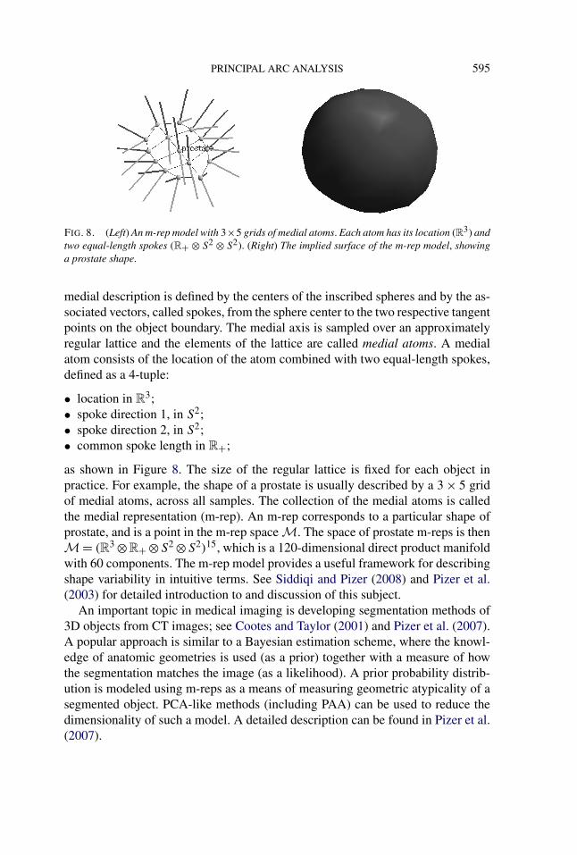
FIG. 8. (Left) An m-rep model with 3×5 grids of medial atoms. Each atom has its location (R3) andtwo equal-length spokes (R+ ⊗ S2 ⊗ S2). (Right) The implied surface of the m-rep model, showinga prostate shape.

medial description is defined by the centers of the inscribed spheres and by the as-sociated vectors, called spokes, from the sphere center to the two respective tangentpoints on the object boundary. The medial axis is sampled over an approximatelyregular lattice and the elements of the lattice are called medial atoms. A medialatom consists of the location of the atom combined with two equal-length spokes,defined as a 4-tuple:

• location in R3;

• spoke direction 1, in S2;• spoke direction 2, in S2;• common spoke length in R+;

as shown in Figure 8. The size of the regular lattice is fixed for each object inpractice. For example, the shape of a prostate is usually described by a 3 × 5 gridof medial atoms, across all samples. The collection of the medial atoms is calledthe medial representation (m-rep). An m-rep corresponds to a particular shape ofprostate, and is a point in the m-rep space M. The space of prostate m-reps is thenM = (R3 ⊗R+ ⊗S2 ⊗S2)15, which is a 120-dimensional direct product manifoldwith 60 components. The m-rep model provides a useful framework for describingshape variability in intuitive terms. See Siddiqi and Pizer (2008) and Pizer et al.(2003) for detailed introduction to and discussion of this subject.

An important topic in medical imaging is developing segmentation methods of3D objects from CT images; see Cootes and Taylor (2001) and Pizer et al. (2007).A popular approach is similar to a Bayesian estimation scheme, where the knowl-edge of anatomic geometries is used (as a prior) together with a measure of howthe segmentation matches the image (as a likelihood). A prior probability distrib-ution is modeled using m-reps as a means of measuring geometric atypicality of asegmented object. PCA-like methods (including PAA) can be used to reduce thedimensionality of such a model. A detailed description can be found in Pizer et al.(2007).


5.2. Simulated m-rep object. The data set partly plotted in Figure 1 is from thegenerator discussed in Jeong et al. (2008). It generates random samples of objectswhose shape changes and motions are physically modeled (with some random-ness) by anatomical knowledge of the bladder, prostate and rectum in the malepelvis. Jeong et al. have proposed and used the generator to estimate the probabil-ity distribution model of shapes of human organs.

In the data set of 60 samples of prostate m-reps we studied, the major motionof prostate is a rotation. In some S2 components, the variation corresponding tothe rotation is along a small circle. Therefore, PAA should fit better for this typeof data than principal geodesics. To make this advantage more clear, we also showresults from a data set by removing the location and the spoke length informationfrom the m-reps, the sample space of which is then {S2}30.

We have applied PAA as described in the previous section. The ratios μ/σ ,estimated for the 30 S2 components, are in general large (with minimum 21.2,median 44.1 and maximum 118), which suggests use of small circles to capturethe variation.

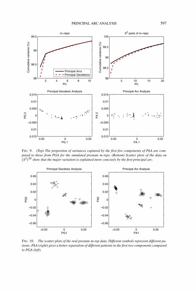
Figure 9 shows the proportion of the cumulative variances, as a function of num-ber of components, from the Principal Geodesic Analysis (PGA) of Fletcher et al.(2004) and PAA. In both cases, the first principal arc leaves smaller residuals thanthe first principal geodesic. What is more important is illustrated in the scatter-plots of the data projected onto the first two principal components. The quadraticform of variation that requires two PGA components is captured by a single PAAcomponent.

The probability distribution model estimated by principal geodesics is qualita-tively different from the distribution estimated by PAA. Although the difference inthe proportion of variance captured is small, the resulting distribution from PAAis no longer elliptical. In this sense, PAA gives a convenient way to describe anonelliptical distribution by, for example, a Normal density.

5.3. Prostate m-reps from real patients. We also have applied PAA to aprostate m-rep data set from real CT images. Our data consist of five patients’image sets, each of which is a series of CT scans containing prostate taken duringa series of radiotherapy treatments [Merck (2008)]. The prostate in each image ismanually segmented by experts and an m-rep model is fitted. The patients, codedas 3106, 3107, 3109, 3112 and 3115, have different numbers of CT scans (17, 12,18, 16 and 15, respectively). We have in total 78 m-reps.

The proportion of variation captured in the first principal arc is 40.89%, slightlyhigher than the 40.53% of the first principal geodesic. Also note that the estimatedprobability distribution model from PAA is different from that of PGA. In par-ticular, PAA gives a better separation of patients in the first two components, asdepicted in the scatter plots (Figure 10).


FIG. 9. (Top) The proportion of variances captured by the first few components of PAA are com-pared to those from PGA for the simulated prostate m-reps. (Bottom) Scatter plots of the data on{S2}30 show that the major variation is explained more concisely by the first principal arc.

FIG. 10. The scatter plots of the real prostate m-rep data. Different symbols represent different pa-tients. PAA (right) gives a better separation of different patients in the first two components comparedto PGA (left).


6. Doubly iterative algorithm to find the least-squares small circle. Wepropose an algorithm to fit the least-squares small circle (1), which is a constrainednonlinear minimization problem. This algorithm is best understood in two iterativesteps: The outer loop approximates the sphere by a tangent space; the inner loopsolves an optimization problem in the linear space, which is much easier thansolving (1) directly. In more detail, the (k + 1)th iteration works as follows. Thesphere is approximated by a tangent plane at ck , the kth solution of the center ofthe small circle. For the points on the tangent plane, any iterative algorithm to finda least-squares circle can be applied as an inner loop. The solution of the inneriteration is mapped back to the sphere and becomes the (k +1)th input of the outerloop operation. One advantage of this algorithm lies in the reduced difficulty ofthe optimization task. The inner loop problem is much simpler than (1) and theouter loop is calculated by a closed-form equation, which leads to a stable andfast algorithm. Another advantage can be obtained by using the exponential mapand log map (12) for the tangent projection, since they preserve the distance fromthe point of tangency to the others, that is, ρ(x, c) = ‖Logc(x)‖ for any x ∈ S2.This is also true for radii of circles. The exponential map transforms a circle inR

2 centered at the origin with radius r to δ(c, r). Thus, whenever (1) reaches itsminimum, the algorithm does not alter the solution.

We first illustrate necessary building blocks of the algorithm. A tangent planeTc at c can be defined for any c in S2, and an appropriate coordinate system of Tcis obtained as follows. Basically, any two orthogonal complements of the directionc can be used as coordinates of Tc. For example, when c = (0,0,1)′ ≡ e3, a coor-dinate system is given by e1 and e2. For a general c, let qc be a rotation operatoron R

3 that maps c to e3. Then a coordinate system for Tc is given by the inverse ofqc applied to e1 and e2, which is equivalent to applying qc to each point of S2 andusing e1, e2 as coordinates.

The rotation operator qc can be represented by a rotation matrix. For c =(cx, cy, cz)

′, the rotation qc is equivalent to rotation through the angle θ =cos−1(cz) about the axis u = (cy,−cx,0)′/

√1 − c2

z , whenever c �= ±e3. Whenc = ±e3, u is set to be e1. It is well known that a rotation matrix with axisu = (ux, uy, uz)

′ and angle θ in radians is, for c = cos(θ), s = sin(θ) and v =1 − cos(θ),

Rc =⎛⎝ c + u2

xv uxuyv − uzs uxuzv + uys

uxuyv + uzs c + u2yv uyuzv − uxs

uxuzv − uys uyuzv + uxs c + u2zv

⎞⎠ ,(11)

so that qc(x) = Rcx, for x ∈ R3.

With the coordinate system for Tc, we shall define the exponential map Expc,a mapping from Tc to S2, and the log map Logc = Exp−1

c . These are defined forv = (v1, v2) ∈ R

2 and x = (x1, x2, x3)′ ∈ S2, as

Expc(v) = qc ◦ Expe3(v), Logc(x) = Loge3

◦qc(x),(12)


for θ = cos−1(x3). See (18)–(19) in the Appendix for Expe3and Loge3

. Note thatLogc(c) = 0 and Logc is not defined for the antipodal point of c.

Once we have approximated each xi by Logc(xi ) ≡ xi , the inner loop finds theminimizer (v, r) of

minn∑

i=1

(‖xi − v‖ − r)2,(13)

which is to find the least-squares circle centered at v with radius r . The generalcircle fitting problem is discussed in, for example, Umbach and Jones (2003) andChernov (2010). This problem is much simpler than (1) because it is an uncon-strained problem and the number of parameters to optimize is decreased by 1.Moreover, optimal solution of r is easily found as

r = 1

n

n∑i=1

‖xi − v‖,(14)

when v is given. Note that for great circle fitting, we can simply put r = π/2. Al-though the problem is still nonlinear, one can use any optimization method thatsolves nonlinear least squares problems. We use the Levenberg–Marquardt algo-rithm, modified by Fletcher (1971) [see Chapter 4 of Scales (1985) and Chapter 3of Bates and Watts (1988)], to minimize (13) with r replaced by r . One can alwaysuse v = 0 as an initial guess since 0 = Logc(c) is the solution from the previous(outer) iteration.

The algorithm is now summarized as follows:

(1) Given {x1, . . . ,xn}, c0 = x1.(2) Given ck , find a minimizer v of (13) with r replaced by (14), with inputs

xi = Logck(xi ).

(3) If ‖v‖ < ε, then iteration stops with the solution c = ck , r = r as in (14).Otherwise, ck+1 = Expck

(v) and go to step 2.

Note that the radius of the fitted circle in Tc is the same as the radius of theresulting small circle. There could be many variations of this algorithm: as aninstance, one can elaborate the initial value selection by using the eigenvector ofthe sample covariance matrix of xi ’s, corresponding to the smallest eigenvalue asdone in Gray, Geiser and Geiser (1980). Experience has shown that the proposedalgorithm is stable and speedy enough. Gray, Geiser and Geiser proposed to solve(1) directly, which seems to be unstable in some cases.

The idea of the doubly iterative algorithm can be applied to other optimizationproblems on manifolds. For example, the geodesic mean is also a solution of anonlinear minimization, where the nonlinearity comes from the use of the geodesicdistance. This can be easily solved by an iterative approximation of the manifold toa linear space [See Chapter 4 of Fletcher (2004)], which is the same as the gradientdescent algorithms [Pennec (2006), Le (2001)]. Note that the proposed algorithm,like other iterative algorithms, only finds one solution even if there are multiplesolutions.


APPENDIX: SOME BACKGROUND ON DIRECT PRODUCT MANIFOLD

We give some necessary geometric background on direct product manifolds.Precise definitions and geometric discussions on a richer class of manifold, Rie-mannian manifold, can be found in Boothby (1986) and Helgason (2001).

A d-dimensional manifold can be thought of as a curved surface embedded ina Euclidean space of higher dimension d ′ (≥d). The manifold is required to besmooth, that is, infinitely differentiable, so that a sufficiently small neighborhoodof any point on the manifold can be well approximated by a linear space. Thetangent space at a point p of a manifold M , TpM , is defined as a linear space ofdimension d which is tangent to M at p. The notion of distance on M is handledby a Riemannian metric, which is a metric of tangent spaces. In particular, thegeodesic distance function ρM(p,q) is roughly defined as the length of the shortestcurve joining p,q ∈ M .

Now consider a direct product manifold M = M1 ⊗ · · · ⊗ Mm. We restrict ourattention to the case where each Mi is one of the simple manifolds S1, S2,R+ orR, but most of the assertions below apply equally well to direct products of moregeneral manifolds.

Geodesic distance function. The geodesic distance between p ≡ (p1, . . . , pm)

and q ≡ (q1, . . . , qm) is defined by

ρM(p,q) =(

m∑i=1

ρ2Mi

(pi, qi)

)1/2

,

where each ρMiis the geodesic distance function on Mi . The geodesic distance

on S1 is defined by the length of the shortest arc. Similarly, the geodesic distanceon S2 is defined by the length of the shortest great circle segment. The geodesicdistance on R+ needs special treatment. In many practical applications, R+ rep-resents a space of scale parameters. A desirable property for a metric on scaleparameters is scale invariance, ρ(rx, ry) = ρ(x, y) for any x, y, r ∈ R+. This canbe achieved by differencing the logs, that is,

ρR+(x, y) =∣∣∣∣ log

x

y

∣∣∣∣ for x, y ∈ R+.(15)

Finally, the geodesic distance on a simple manifold R or Rd is the Euclidean dis-

tance.Geodesic mean and variance. The geodesic mean of a set of points in M , also

referred to as the intrinsic mean, is also calculated component-wise. The geodesicmean of x1, . . . , xn ∈ M is the minimizer in M of the sum of squared geodesicdistances to the data. Thus, the geodesic mean is defined as

x = argminx∈M

1

n

n∑i=1

ρ2M(x, xi).(16)


In fact, each xi of x = (x1, . . . , xm) is the geodesic mean of xi1, . . . , x

in ∈ Mi . The

geodesic mean of θ1, . . . , θn ∈ [0,2π) ∼= S1 is found by examining a candidate setconsisting of

θj =∑n

i=1 θi + 2jπ

n, j = 0, . . . , n − 1,(17)

as in Moakher (2002). The geodesic mean in S2 can be calculated by a full gridsearch or an iterative algorithm, as described in Section 6. The geodesic mean inR+ or R is straightforward. Note that the geodesic mean may not be unique. How-ever, throughout the paper, we have assumed that the data have a unique geodesicmean which is true in most data analytic situations. Statistical investigation of thegeodesic mean on manifolds can be found, for example, in Bhattacharya and Pa-trangenaru (2003, 2005) and Le and Kume (2000).

A related notion is geodesic variance. A sample geodesic variance is de-fined by the average squared geodesic distances to the geodesic mean, that is,1n

∑ni=1 ρ2

M(x, xi). When M is indeed the Euclidean space, the geodesic varianceis the same as the total variance (the trace of the variance–covariance matrix).

Mappings to tangent space. The exponential map maps a point in TpM to M .The log map is the inverse exponential map whose domain is in M . For a directproduct manifold M , the mappings are also defined component-wise. For S1, letθ ∈ R denote an element of TpS1 where p is set to be (1,0) ∈ S1 embedded in R

2.Then the exponential map is defined as

Expp(θ) = (cos θ, sin θ).

The corresponding log map of x = (x1, x2) is defined as Logp(x) = sign(x2) ·arccos(x1). For S2, let v = (v1, v2) denote a tangent vector in TpS2. Let p = e3,then the exponential map Expp :TpS2 −→ S2 is defined by

Expp(v) =(

v1

‖v‖ sin‖v‖, v2

‖v‖ sin‖v‖, cos‖v‖).(18)

This equation can be understood as a rotation of the base point p to the directionof v with angle ‖v‖. The corresponding log map for a point x = (x1, x2, x3) ∈ S2

is given by

Logp(x) =(x1

θ

sin θ, x2

θ

sin θ

),(19)

where θ = arccos(x3) is the geodesic distance from p to x. Note that the antipo-dal point of p is not in the domain of the log map, that is, the domain of Logp isS2/{−p}. In both S1 and S2, p can be set to be any point on S1 or S2. The ex-ponential and log map for an arbitrary Tp can be defined together with a rotationoperator, which is defined in Section 6 for the case of S2. The exponential map ofR+ is defined by the standard real exponential function. The domain of the inverseexponential map, the log map, is R+ itself. Finally, the exponential map on R isthe identity map.


REFERENCES

BATES, D. M. and WATTS, D. G. (1988). Nonlinear Regression Analysis and Its Applications.Wiley Series in Probability and Mathematical Statistics: Applied Probability and Statistics. Wiley,New York. MR1060528

BHATTACHARYA, R. and PATRANGENARU, V. (2003). Large sample theory of intrinsic and extrinsicsample means on manifolds. I. Ann. Statist. 31 1–29. MR1962498

BHATTACHARYA, R. and PATRANGENARU, V. (2005). Large sample theory of intrinsic and extrinsicsample means on manifolds. II. Ann. Statist. 33 1225–1259. MR2195634

BINGHAM, C. and MARDIA, K. V. (1978). A small circle distribution on the sphere. Biometrika 65379–389. MR0513936

BOOTHBY, W. M. (1986). An Introduction to Differentiable Manifolds and Riemannian Geometry,2nd ed. Academic Press, Orlando, FL. MR0861409

CHERNOV, N. (2010). Circular and Linear Regression: Fitting Circles and Lines by Least Squares.Chapman & Hall/CRC Press, Boca Raton, FL.

CHURCHILL, R. V. and BROWN, J. W. (1984). Complex Variables and Applications, 4th ed.McGraw-Hill, New York. MR0730937

COOTES, T. F. and TAYLOR, C. J. (2001). Statistical models of appearance for medical image analy-sis and computer vision. In Medical Imaging 2001: Image Processing (M. Sonka and K. M. Han-son, eds.). Proceedings of the SPIE 4322 236–248. SPIE.

COX, D. R. (1969). Some sampling problems in technology. In New Developments in Survey Sam-pling (U. L. Johnson and H. Smith, eds.). Wiley, New York.

ELANDT, R. C. (1961). The folded normal distribution: Two methods of estimating parameters frommoments. Technometrics 3 551–562. MR0130738

FISHER, N. I. (1993). Statistical Analysis of Circular Data. Cambridge Univ. Press, Cambridge.MR1251957

FISHER, N. I., LEWIS, T. and EMBLETON, B. J. J. (1993). Statistical Analysis of Spherical Data.Cambridge Univ. Press, Cambridge. MR1247695

FLETCHER, R. (1971). A modified Marquardt subroutine for non-linear least squares. TechnicalReport AERE-R 6799.

FLETCHER, P. T. (2004). Statistical variability in nonlinear spaces: Application to shape analysisand DT-MRI. PhD thesis, Univ. North Carolina at Chapel Hill.

FLETCHER, P. T., LU, C., PIZER, S. M. and JOSHI, S. (2004). Principal geodesic analysis for thestudy of nonlinear statistics of shape. IEEE Trans. Med. Imaging 23 995–1005.

GRAY, N. H., GEISER, P. A. and GEISER, J. R. (1980). On the least-squares fit of small and greatcircles to spherically projected orientation data. Math. Geol. 12 173–184. MR0593408

HASTIE, T. and STUETZLE, W. (1989). Principal curves. J. Amer. Statist. Assoc. 84 502–516.MR1010339

HELGASON, S. (2001). Differential Geometry, Lie Groups, and Symmetric Spaces. Graduate Studiesin Mathematics 34. Amer. Math. Soc., Providene, RI. MR1834454

HUCKEMANN, S., HOTZ, T. and MUNK, A. (2010). Intrinsic shape analysis: Geodesic PCA forRiemannian manifolds modulo isometric lie group actions. Statist. Sinica 20 1–58. MR2640651

HUCKEMANN, S. and ZIEZOLD, H. (2006). Principal component analysis for Riemannian man-ifolds, with an application to triangular shape spaces. Adv. in Appl. Probab. 38 299–319.MR2264946

JEONG, J.-Y., STOUGH, J. V., MARRON, J. S. and PIZER, S. M. (2008). Conditional-mean ini-tialization using neighboring objects in deformable model segmentation. In Medical Imaging2008: Image Processing (J. M. Reinhardt and J. P. W. Pluim, eds.). Proceedings of the SPIE6914 69144R.1–69144R.9. SPIE.

JOHNSON, N. L. (1962). The folded normal distribution: Accuracy of estimation by maximum like-lihood. Technometrics 4 249–256. MR0137221

http://www.ams.org/mathscinet-getitem?mr=1060528
















KARCHER, H. (1977). Riemannian center of mass and mollifier smoothing. Comm. Pure Appl. Math.30 509–541. MR0442975

KRANTZ, S. G. (1999). Handbook of Complex Variables. Birkhäuser, Boston, MA. MR1738432LE, H. (2001). Locating Fréchet means with application to shape spaces. Adv. in Appl. Probab. 33

324–338. MR1842295LE, H. and KUME, A. (2000). The Fréchet mean shape and the shape of the means. Adv. in Appl.

Probab. 32 101–113. MR1765168LEONE, F. C., NELSON, L. S. and NOTTINGHAM, R. B. (1961). The folded normal distribution.

Technometrics 3 543–550. MR0130737MARDIA, K. V. and GADSDEN, R. J. (1977). A circle of best fit for spherical data and areas of

vulcanism. J. Roy. Statist. Soc. Ser. C 26 238–245.MARDIA, K. V. and JUPP, P. E. (2000). Directional Statistics. Wiley Series in Probability and Sta-

tistics. Wiley, Chichester. MR1828667MERCK, S. M., TRACTON, G., SABOO, R., LEVY, J., CHANEY, E., PIZER, S. M. and JOSHI, S.

(2008). Training models of anatomic shape variability. Med. Phys. 35 3584–3596.MOAKHER, M. (2002). Means and averaging in the group of rotations. SIAM J. Matrix Anal. Appl.

24 1–16 (electronic). MR1920548PENNEC, X. (2006). Intrinsic statistics on Riemannian manifolds: Basic tools for geometric mea-

surements. J. Math. Imaging Vision 25 127–154.PIZER, S. M., FLETCHER, P. T., FRIDMAN, Y., FRITSCH, D. S., GASH, A. G., GLOTZER, J. M.,

JOSHI, S., THALL, A., TRACTON, G., YUSHKEVICH, P. and CHANEY, E. L. (2003). De-formable m-reps for 3D medical image segmentation. Int. J. Comput. Vision 55 85–106.

PIZER, S. M., BROADHURST, R. E., LEVY, J., LIU, X., JEONG, J.-Y., STOUGH, J., TRACTON, G.and CHANEY, E. L. (2007). Segmentation by posterior optimization of m-reps: Strategy andresults. Unpublished manuscript.

RIVEST, L.-P. (1999). Some linear model techniques for analyzing small-circle spherical data.Canad. J. Statist. 27 623–638. MR1745827

SCALES, L. E. (1985). Introduction to Nonlinear Optimization. Springer, New York. MR0776609SIDDIQI, K. and PIZER, S. (2008). Medial Representations: Mathematics, Algorithms and Applica-

tions. Springer, New York. MR2547467UMBACH, D. and JONES, K. N. (2003). A few methods for fitting circles to data. IEEE Transactions

on Instrumentation and Measurement 52 1881–1885.

S. JUNG

J. S. MARRON

DEPARTMENT OF STATISTICS

AND OPERATIONS RESEARCH

UNIVERSITY OF NORTH CAROLINA

CHAPEL HILL, NORTH CAROLINA 27599USAE-MAIL: [email protected]

[email protected]

M. FOSKEY

DEPARTMENT OF RADIATION ONCOLOGY

UNIVERSITY OF NORTH CAROLINA

CHAPEL HILL, NORTH CAROLINA 27599USAE-MAIL: [email protected]











mailto:[email protected]



principal arc analysis on direct product manifolds · principal arc analysis on direct product ......

Documents