princeton university...madness of people” internet bubble (1992 –2000) druckenmiller of soros’...
TRANSCRIPT

Princeton University

Bru
nn
erm
eier
Systemic risk build-up during (credit) bubble … and materializes in a crisis “Volatility Paradox” contemp. measures inappropriate
Spillovers/contagion – externalities Direct contractual: domino effect (interconnectedness)
Indirect: price effect (fire-sale externalities) credit crunch, liquidity spirals
Adverse GE response amplification, persistence
Systemic risk –a broad definition
2
Loss of
net worth
Shock to
capital
Precaution
+ tighter
margins
volatility
price
Fire
sales
pre
ve
ntive
crisis
man
ag
em
ent

Princeton University

Bru
nn
erm
eier
Internet bubble - 1990’s
Why do bubbles persist?
Do professional traders ride the bubble or attack the bubble (go short)?
What happened in March 2000?6
Loss of ca. 60 %
from high of $ 5,132
Loss of ca. 85 %
from high of Euro 8,583

Bru
nn
erm
eier
Credit bubble 2004-2006
7

Bru
nn
erm
eier
US House price index –Case-Shiller
8
Bru
nn
erm
eier
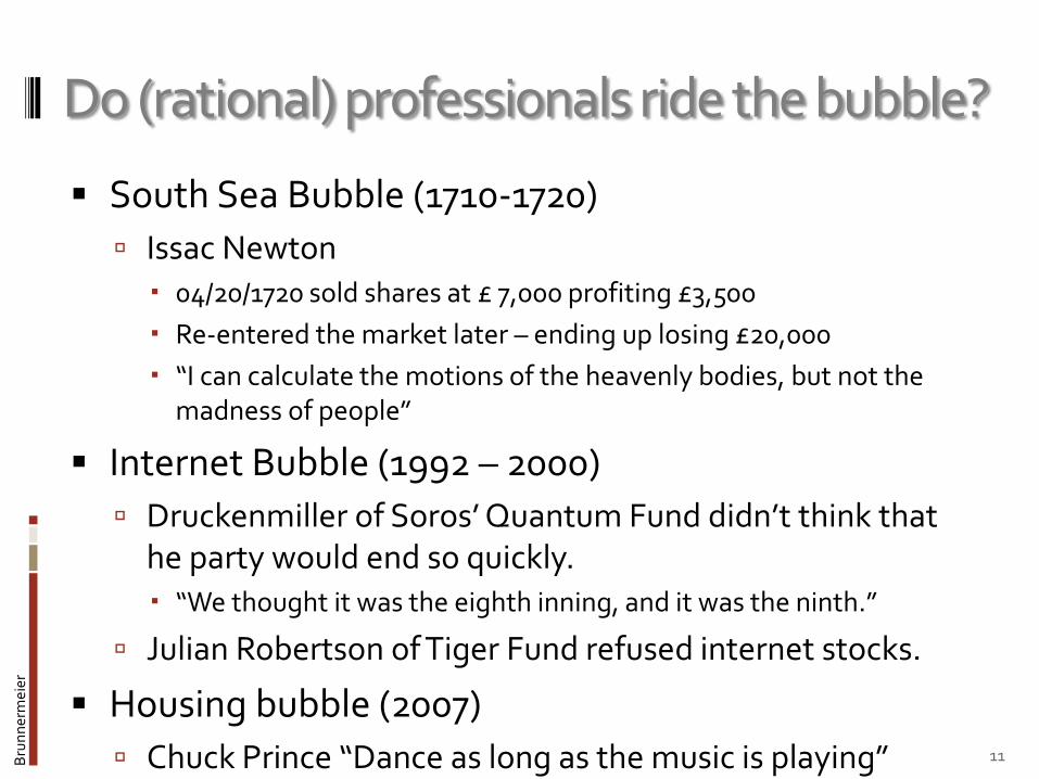
Do (rational) professionals ride the bubble?
South Sea Bubble (1710-1720)
Issac Newton 04/20/1720 sold shares at £ 7,000 profiting £3,500
Re-entered the market later – ending up losing £20,000
“I can calculate the motions of the heavenly bodies, but not the madness of people”
Internet Bubble (1992 – 2000)
Druckenmiller of Soros’ Quantum Fund didn’t think that he party would end so quickly. “We thought it was the eighth inning, and it was the ninth.”
Julian Robertson of Tiger Fund refused internet stocks.
Housing bubble (2007)
Chuck Prince “Dance as long as the music is playing” 11

Bru
nn
erm
eier
Stylized facts
Initial innovation justifies some price increase
Momentum leads to price overshooting
Extrapolative expectations
Many market participants seem to be aware that the “price is too high” but keep on holding the asset
“Play as long as the music is playing”
Resell-option is crucial for speculative bubbles
Minksy moment – triggered by “trivial news”
Credit bubbles lead to extra amplification effects in downturn (since they can impair financial sector)
subprime borrowing was only 4% of US mortgage market
Amplification focus of next lecture
13

Bru
nn
erm
eier
Minsky moment –Wile E. Coyote Effect
14
Bru
nn
erm
eier
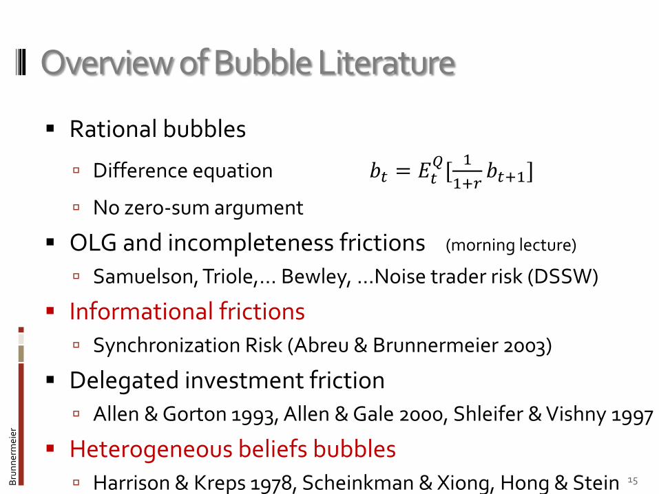
Overview of Bubble Literature
Rational bubbles
Difference equation 𝑏𝑡 = 𝐸𝑡𝑄[
1
1+𝑟𝑏𝑡+1]
No zero-sum argument
OLG and incompleteness frictions (morning lecture)
Samuelson, Triole,… Bewley, …Noise trader risk (DSSW)
Informational frictions
Synchronization Risk (Abreu & Brunnermeier 2003)
Delegated investment friction
Allen & Gorton 1993, Allen & Gale 2000, Shleifer & Vishny 1997
Heterogeneous beliefs bubbles
Harrison & Kreps 1978, Scheinkman & Xiong, Hong & Stein 15

Bru
nn
erm
eier
On Market Efficiency
Keynes (1936) ) bubble can emerge
“It might have been supposed that competition between expert professionals, possessing judgment and knowledge beyond that of the average private investor, would correct the vagaries of the ignorant individual left to himself.”
Friedman (1953), Fama (1965)
Efficient Market Hypothesis ) no bubble emerges
“If there are many sophisticated traders in the market, they may cause these “bubbles” to burst before they really get under way.”
16
Bru
nn
erm
eier
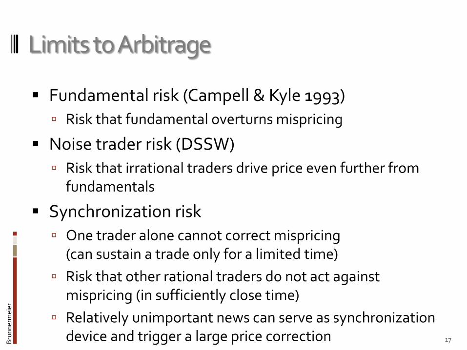
Limits to Arbitrage
Fundamental risk (Campell & Kyle 1993)
Risk that fundamental overturns mispricing
Noise trader risk (DSSW)
Risk that irrational traders drive price even further from fundamentals
Synchronization risk
One trader alone cannot correct mispricing(can sustain a trade only for a limited time)
Risk that other rational traders do not act against mispricing (in sufficiently close time)
Relatively unimportant news can serve as synchronization device and trigger a large price correction 17

Bru
nn
erm
eier
Timing Game -Synchronization
(When) will behavioral traders be overwhelmed by rational arbitrageurs?
Collective selling pressure of arbitrageurs more than suffices to burst the bubble.
Rational arbitrageurs understand that an eventualcollapse is inevitable. But when?
Delicate, difficult, dangerous TIMING GAME !
18

Bru
nn
erm
eier
Elements of the Timing Game
Coordination at least 𝜅 > 0 arbs have to be ‘out of the market’
Competition only first 𝜅 < 1 arbs receive pre-crash price.
Profitable ride ride bubble as long as possible.
Sequential Awareness
A Synchronization Problem arises! Absent of sequential awareness
competitive element dominates ) and bubble burst
immediately.
With sequential awarenessincentive to TIME THE MARKET ) “delayed arbitrage”
) persistence of bubble
19
Bru
nn
erm
eier
Overview
Introduction
Model setup
Preliminary analysis
Persistence of bubbles
Public events
Price cascades and rebounds
Empirical evidence & Hedge funds
Brunnermeier & Nagel (2004)
20
Bru
nn
erm
eier
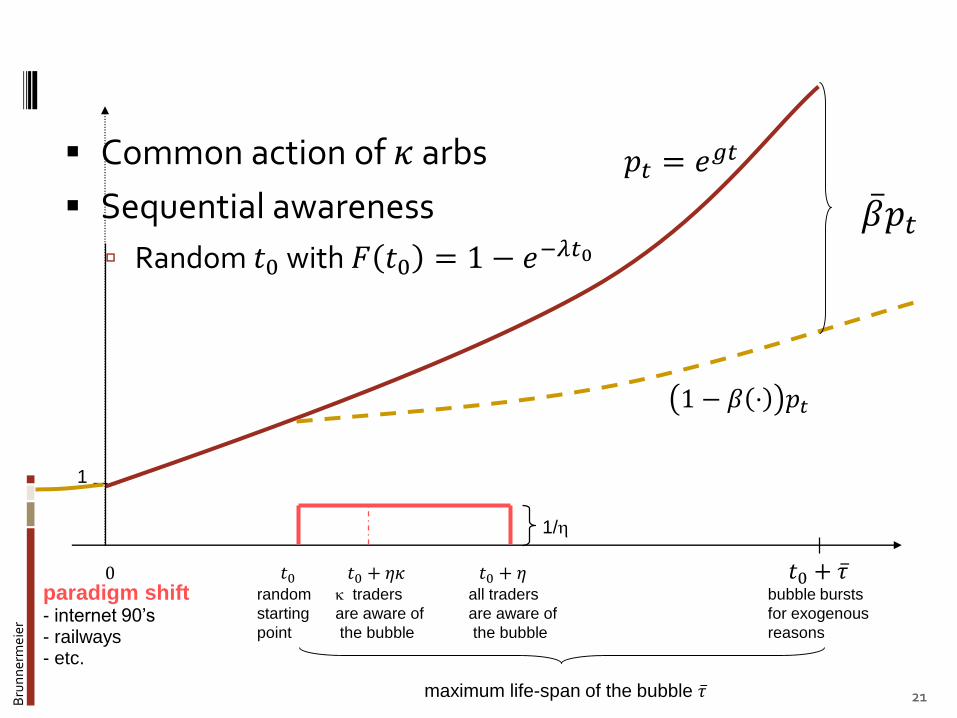
Common action of 𝜅 arbs
Sequential awareness
Random 𝑡0 with 𝐹 𝑡0 = 1 − 𝑒−𝜆𝑡0
2121
𝑡0 𝑡0 + 𝜂𝑡0 + 𝜂𝜅random
starting
point
maximum life-span of the bubble ҧ𝜏
traders
are aware of
the bubble
all traders
are aware of
the bubble
bubble bursts
for exogenous
reasons
1
1/
ҧ𝛽𝑝𝑡
𝑡0 + ҧ𝜏
𝑝𝑡 = 𝑒𝑔𝑡
1 − 𝛽 ⋅ 𝑝𝑡
0paradigm shift- internet 90’s- railways- etc.

Bru
nn
erm
eier
Payoff structure
Focus: “when does bubble burst”
𝑡0 is only random variables, all other variables are CK
Cash payoff (difference)
Sell one share at 𝑡 − Δ instead of at 𝑡
𝑝𝑡−Δ𝑒𝑟Δ − 𝑝𝑡
where 𝑝𝑡 = ൝𝑒𝑔𝑡 prior to crash
1 − 𝛽 𝑡 − 𝑡0 𝑒𝑔𝑡 after the crash
Price at the time of bursting (tie breaking rule) Pre crash price for first random orders up to 𝜅
22

Bru
nn
erm
eier
Payoff structure, Trading
Small transaction costs 𝑐𝑒𝑟𝑡
Risk-neutrality but max/min stock position
Max long position
Max short position
Due to capital constraints, margin requirements etc.
Definition 1: trading equilibrium
Perfect Bayesian Nash Equilibrium
Belief restriction: trader who attacks at time 𝑡 believes that all traders who became aware of the bubble prior to her also attack at 𝑡.
23

Bru
nn
erm
eier
Sell out condition for Δ→ 0periods
Sell out at 𝑡ifΔℎ 𝑡 𝑡𝑖 𝐸𝑡 𝛽𝑝𝑡 ⋅ ≥ (1 − Δℎ 𝑡 𝑡𝑖 𝑔 − 𝑟 𝑝𝑡Δ
ℎ 𝑡 𝑡𝑖 ≥𝑔 − 𝑟
𝛽∗
RHS → 𝑔 − 𝑟 as 𝑡 → ∞
Bursting date: 𝑇∗ 𝑡0 = min{𝑇 𝑡0 + 𝜂𝜅 , 𝑡0 + ҧ𝜏}24
appreciation rate
benefit of attacking cost of attacking

Bru
nn
erm
eier
Sequential awareness
25
𝑡
Distribution of 𝑡0 Distribution of 𝑡0 + ҧ𝜏(bursting if nobody attacks)
𝑡0 𝑡0 + ҧ𝜏
𝑡𝑖𝑡𝑖 − 𝜂
since 𝑡𝑖 ≤ 𝑡0 + 𝜂 since 𝑡𝑖 ≥ 𝑡0
trader 𝑡𝑖

Bru
nn
erm
eier
Sequential awareness
26
since 𝑡𝑖 ≤ 𝑡0 + 𝜂 since 𝑡𝑖 ≥ 𝑡0
t
Distribution of 𝑡0 Distribution of 𝑡0 + ҧ𝜏(bursting if nobody attacks)
𝑡0 𝑡0 + ҧ𝜏
𝑡𝑖𝑡𝑖 − 𝜂
𝑡𝑗 − 𝜂 𝑡𝑗
trader 𝑡𝑖
trader 𝑡𝑗
𝑡

Bru
nn
erm
eier
Sequential awareness
27
trader 𝑡𝑖
𝑡0 𝑡0 + ҧ𝜏𝑡𝑘
t
trader 𝑡𝑗
t
trader 𝑡𝑘
Distribution of 𝑡0 Distribution of 𝑡0 + ҧ𝜏(bursting if nobody attacks)
𝑡𝑖 − 𝜂
𝑡𝑗 − 𝜂 𝑡𝑗
𝑡𝑖since 𝑡𝑖 ≤ 𝑡0 + 𝜂 since 𝑡𝑖 ≥ 𝑡0
𝑡

Bru
nn
erm
eier
Conjecture 1: Immediate attack
28
) Bubble bursts at 𝒕𝟎 + 𝜼𝜿when 𝜅 traders are aware of the bubble
𝑡𝑖 − 𝜂 𝑡𝑖𝑡
Bru
nn
erm
eier
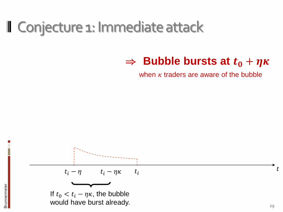
Conjecture 1: Immediate attack
29
) Bubble bursts at 𝒕𝟎 + 𝜼𝜿when 𝜅 traders are aware of the bubble
If 𝑡0 < 𝑡𝑖 − 𝜂𝜅, the bubble
would have burst already.
𝑡𝑖 − 𝜂 𝑡𝑖 − 𝜂𝜅 𝑡𝑖𝑡

Bru
nn
erm
eier
Conjecture 1: Immediate attack
30
) Bubble bursts at 𝒕𝟎 + 𝜼𝜿when 𝜅 traders are aware of the bubble
/(1-e-)
𝑡𝑖 − 𝜂 𝑡𝑖 − 𝜂𝜅 𝑡𝑖 + 𝜂𝜅𝑡𝑖
Distribution of 𝑡0
𝑡

Bru
nn
erm
eier
Conjecture 1: Immediate attack
31
) Bubble bursts at 𝒕𝟎 + 𝜼𝜿when 𝜅 traders are aware of the bubble
/(1-e-)
Distribution of 𝑡0
𝑡𝑖 − 𝜂 𝑡𝑖 − 𝜂𝜅 𝑡𝑖 + 𝜂𝜅𝑡𝑖𝑡
Bru
nn
erm
eier
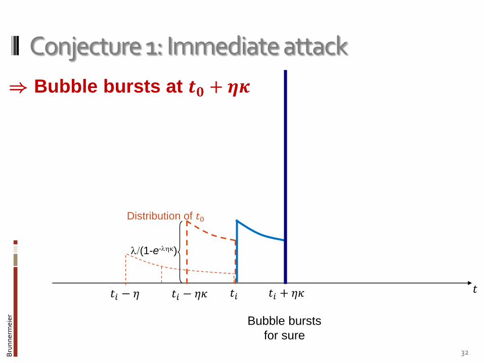
Conjecture 1: Immediate attack
32
/(1-e-)
Bubble bursts
for sure
) Bubble bursts at 𝒕𝟎 + 𝜼𝜿
𝑡𝑖 − 𝜂 𝑡𝑖 − 𝜂𝜅 𝑡𝑖 + 𝜂𝜅𝑡𝑖
Distribution of 𝑡0
𝑡

Bru
nn
erm
eier
Conjecture 1: Immediate attack
33
/(1-e-)
Bubble bursts
for sure
) Bubble bursts at 𝒕𝟎 + 𝜼𝜿
𝑡𝑖 − 𝜂 𝑡𝑖 − 𝜂𝜅 𝑡𝑖 + 𝜂𝜅𝑡𝑖
Distribution of 𝑡0
𝑡

Bru
nn
erm
eier
Conjecture 1: Immediate attack
34
/(1-e-)
Bubble bursts
for sure
) Bubble bursts at 𝒕𝟎 + 𝜼𝜿
𝑡𝑖 − 𝜂 𝑡𝑖 − 𝜂𝜅 𝑡𝑖 + 𝜂𝜅𝑡𝑖
Distribution of 𝑡0
𝑡

Bru
nn
erm
eier
Conjecture 1: Immediate attack
35
) Bubble bursts at 𝒕𝟎 + 𝜼𝜿
hazard rate of the bubble
ℎ =𝜆
1 − 𝑒−𝜆 𝑡𝑖+𝜂𝜅−𝑡
𝜆
1 − 𝑒𝜆𝜂𝜅
𝑡𝑖 − 𝜂 𝑡𝑖 − 𝜂𝜅 𝑡𝑖 + 𝜂𝜅𝑡𝑖
Distribution of 𝑡0
𝑡

Bru
nn
erm
eier
Conjecture 1: Immediate attack
36
) Bubble bursts at 𝒕𝟎 + 𝜼𝜿
hazard rate of the bubble
ℎ =𝜆
1 − 𝑒−𝜆 𝑡𝑖+𝜂𝜅−𝑡
𝜆
1 − 𝑒𝜆𝜂𝜅
Recall the sell out condition:
ℎ 𝑡 𝑡𝑖 ≥𝑔 − 𝑟
𝛽∗
𝑡𝑖 − 𝜂 𝑡𝑖 − 𝜂𝜅 𝑡𝑖 + 𝜂𝜅𝑡𝑖
Distribution of 𝑡0
𝑡
Bru
nn
erm
eier
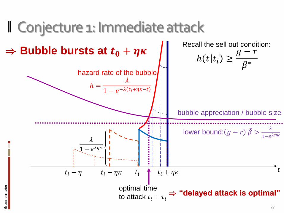
Conjecture 1: Immediate attack
37
) Bubble bursts at 𝒕𝟎 + 𝜼𝜿
hazard rate of the bubble
ℎ =𝜆
1 − 𝑒−𝜆 𝑡𝑖+𝜂𝜅−𝑡
𝜆
1 − 𝑒𝜆𝜂𝜅
optimal time
to attack 𝑡𝑖 + 𝜏𝑖) “delayed attack is optimal”
bubble appreciation / bubble size
Recall the sell out condition:
ℎ 𝑡 𝑡𝑖 ≥𝑔 − 𝑟
𝛽∗
lower bound: 𝑔 − 𝑟 ҧ𝛽 >𝜆
1−𝑒𝜆𝜂𝜅
𝑡𝑖 − 𝜂 𝑡𝑖 − 𝜂𝜅 𝑡𝑖 + 𝜂𝜅𝑡𝑖𝑡

Bru
nn
erm
eier
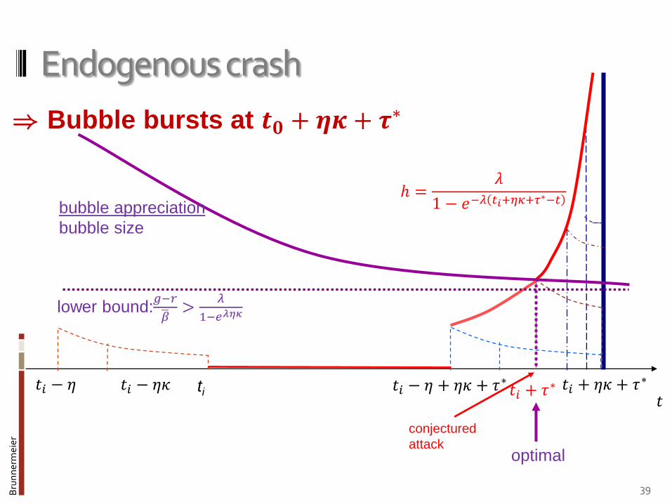
Endogenous Crash for large enough ҧ𝜏 (i.e. ҧ𝛽)
Proposition 3: Suppose 𝜆
1−𝑒−𝜆𝜂𝜅>
𝑔−𝑟
ഥ𝛽
Unique trading equilibrium
Traders begin attacking after a delay of 𝜏∗ periods
Bubble bursts due to endogenous selling pressure at a size of 𝑝𝑡 times
𝛽∗ =1 − 𝑒−𝜆𝜂𝜅
𝜆𝑔 − 𝑟
38
Bru
nn
erm
eier
Endogenous crash
39
) Bubble bursts at 𝒕𝟎 + 𝜼𝜿 + 𝝉∗
ti
optimal
conjectured
attack
bubble appreciation
bubble size
ℎ =𝜆
1 − 𝑒−𝜆 𝑡𝑖+𝜂𝜅+𝜏∗−𝑡
lower bound:𝑔−𝑟ഥ𝛽
>𝜆
1−𝑒𝜆𝜂𝜅
𝑡𝑖 − 𝜂 𝑡𝑖 − 𝜂𝜅 𝑡𝑖 + 𝜂𝜅 + 𝜏∗𝑡𝑖 + 𝜏∗𝑡𝑖 − 𝜂 + 𝜂𝜅 + 𝜏∗
𝑡

Bru
nn
erm
eier
Exogenous crash for low ҧ𝜏 (i.e. low ҧ𝛽)
Proposition 2: Suppose 𝜆
1−𝑒−𝜆𝜂𝜅≤
𝑔−𝑟
ഥ𝛽.
Unique trading equilibrium
Traders begin attacking after a delay of𝜏1 < ҧ𝜏 periods.
Bubble does not burst due to endogenous selling pressure prior to 𝑡0 + ҧ𝜏.
40

Bru
nn
erm
eier
Lack of common knowledge
44
𝑡0 𝑡0 + 𝜂𝜅
) standard backwards induction can’t be applied
𝑡0 + 𝜂
everybody
knows of the
the bubble
𝜅 traders
know of
the bubble
everybody knows that
everybody knows of the
bubble
everybody knows that
everybody knows that
everybody knows of
the bubble
(same reasoning applies for 𝜅 traders)
…
…
endogenous burst
𝑡0 + 𝜂𝜅 + 𝜏∗
𝑡0 + ҧ𝜏𝑡0 + 2𝜂 𝑡0 + 3𝜂

Bru
nn
erm
eier
Role of synchronizing events
News may have an impact disproportionate to any intrinsic informational (fundamental) content
News can serve as a synchronization device
Fads & fashion in information
Which news should traders coordinate on?
When “synchronized attach” fails, then the bubble is temporarily strengthened
45

Bru
nn
erm
eier
Setting with synchronizing events
Focus on news with no info content (sunspots)
Synchronizing events occur with Poisson arrival rate
Note that pre-emption argument does not apply since event occurs with zero probability
Arbitrageurs who are aware of the bubble become increasingly worried about it over time.
Only traders who became aware of the bubble more than 𝜏𝑒 periods ago observe (look out for) this synchronizing event.
46

Bru
nn
erm
eier
Synchronizing events – market rebounds
Proposition 5: In ‘responsive equilibrium’Sell out a) always at the time of the public event 𝑡𝑒,
b) after 𝑡𝑖 + 𝜏∗∗ (where 𝜏∗∗ < 𝜏∗)
except after a failed attack at , re-enter the marketfor 𝑡 ∈ 𝑡𝑒 , 𝑡𝑒 − 𝜏𝑒 + 𝜏∗∗ .
Intuition for re-entering the market For 𝑡𝑒 < 𝑡0 + 𝜂𝜅 + 𝜏𝑒 attack fails, agents learn 𝑡0 > 𝑡𝑒 − 𝜏𝑒 − 𝜂𝜅
Without public event, they would have learnt this only at 𝑡𝑒 + 𝜏𝑒 − 𝜏∗∗
Density that bubble burst for endogenous reasons is zero
47

Bru
nn
erm
eier
Conclusion of Bubbles and Crashes
Bubbles
Dispersion of opinion among arbs causes a synchronization problem which makes coordinated price correction difficult.
Arbitrageurs time the market and ride the bubble⇒ Bubbles persist
Crashes
Can be triggered by unanticipated news without any fundamental content, since
It might serve as synchronization device.
Rebound
Can occur after a failed attack which temporarily strengthens the bubble 50
Princeton University and Stanford University
Bru
nn
erm
eier
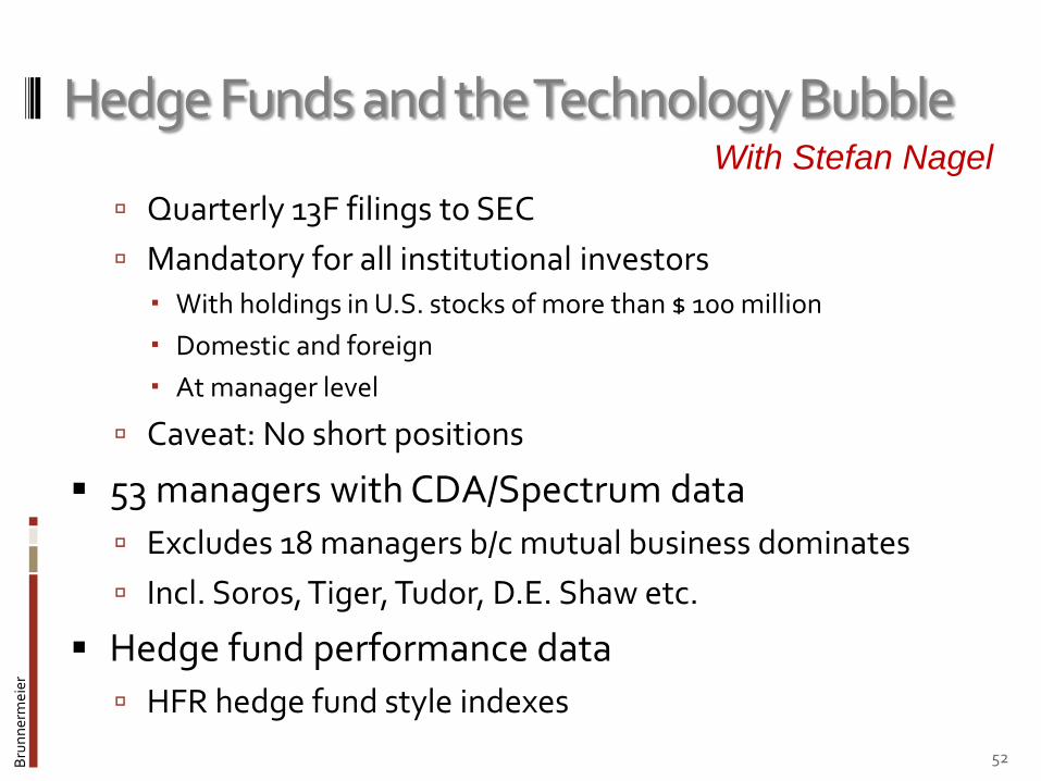
Hedge Funds and the Technology Bubble
Quarterly 13F filings to SEC
Mandatory for all institutional investors With holdings in U.S. stocks of more than $ 100 million
Domestic and foreign
At manager level
Caveat: No short positions
53 managers with CDA/Spectrum data
Excludes 18 managers b/c mutual business dominates
Incl. Soros, Tiger, Tudor, D.E. Shaw etc.
Hedge fund performance data
HFR hedge fund style indexes
52
With Stefan Nagel

Bru
nn
erm
eier
Did hedge funds ride the bubble?
53
Mar-98
Jun-98
Sep-98
Dec-98
Mar-99
Jun-99
Sep-99
Dec-99
Mar-00
Jun-00
Sep-00
Dec-00
Fig. 2: Weight of NASDAQ technology stocks (high P/S) in aggregate hedge fund portfolio versus weight
in market portfolio.
0.00
0.05
0.10
0.15
0.20
0.25
0.30
0.35
Mar-98 Jun-98 Sep-98 Dec-98 Mar-99 Jun-99 Sep-99 Dec-99 Mar-00 Jun-00 Sep-00 Dec-00
Hegde Fund Portfolio Market Portfolio
Proportion invested in NASDAQ high P/S stocks NASDAQ Peak

Bru
nn
erm
eier
Did Soros ride the bubble?
54
Fig. 4a: Weight of technology stocks in hedge fund portfolios versus weight in market portfolio
0.00
0.20
0.40
0.60
0.80
Mar-98 Jun-98 Sep-98 Dec-98 Mar-99 Jun-99 Sep-99 Dec-99 Mar-00 Jun-00 Sep-00 Dec-00
Proportion invested in NASDAQ high P/S stocks
Zw eig-DiMenna
Soros
Husic
Market Portfolio
OmegaTiger

Bru
nn
erm
eier
Fund in- and outflows
55
-0.20
-0.15
-0.10
-0.05
0.00
0.05
0.10
Mar-98 Jun-98 Sep-98 Dec-98 Mar-99 Jun-99 Sep-99 Dec-99 Mar-00 Jun-00 Sep-00 Dec-00
Fund flows as proportion of assets under management
Quantum Fund (Soros)
Jaguar Fund (Tiger)
Bru
nn
erm
eier
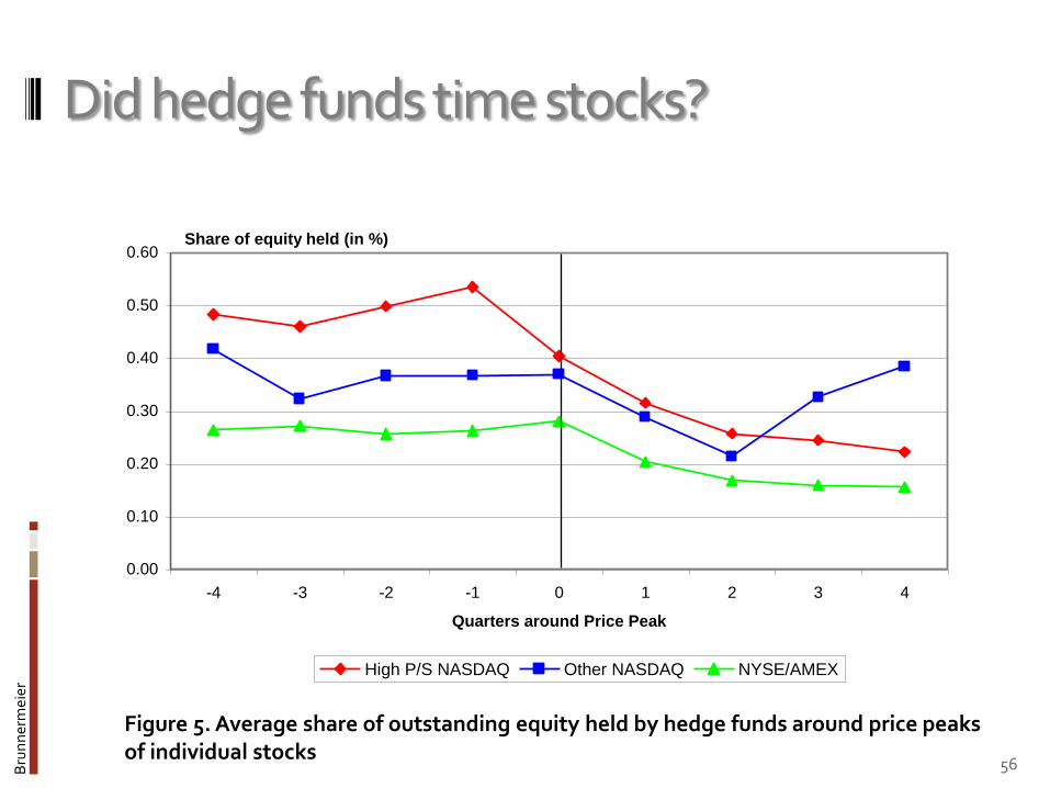
Did hedge funds time stocks?
56
0.00
0.10
0.20
0.30
0.40
0.50
0.60
-4 -3 -2 -1 0 1 2 3 4
Quarters around Price Peak
High P/S NASDAQ Other NASDAQ NYSE/AMEX
Share of equity held (in %)
Figure 5. Average share of outstanding equity held by hedge funds around price peaks of individual stocks

Bru
nn
erm
eier
Did hedge funds’ timing pay off?
57
Mar-98 Jun-98 Sep-98 Dec-98 Mar-99 Jun-99 Sep-99 Dec-99 Mar-00 Jun-00 Sep-00 Dec-00
Total return index
High P/S Copycat Fund All High P/S NASDAQ Stocks
1.0
2.0
3.0
4.0
Figure 6: Performance of a copycat fund that replicates hedge fund holdings in the NASDAQ high P/S segment

Bru
nn
erm
eier
Conclusion
Hedge funds were riding the bubble
Short sale constrains and “arbitrage” risk are not sufficient to explain this behavior.
Timing best of hedge funds were well placed. Outperformance!
Rues out unawareness of bubble
Suggests predictable investor sentiment. Riding the bubble for a while may have been a rational strategy
⇒ Supports ‘bubble-timing’ models
58


Bru
nn
erm
eier
Bubbleswith Trading Cost – simplified example
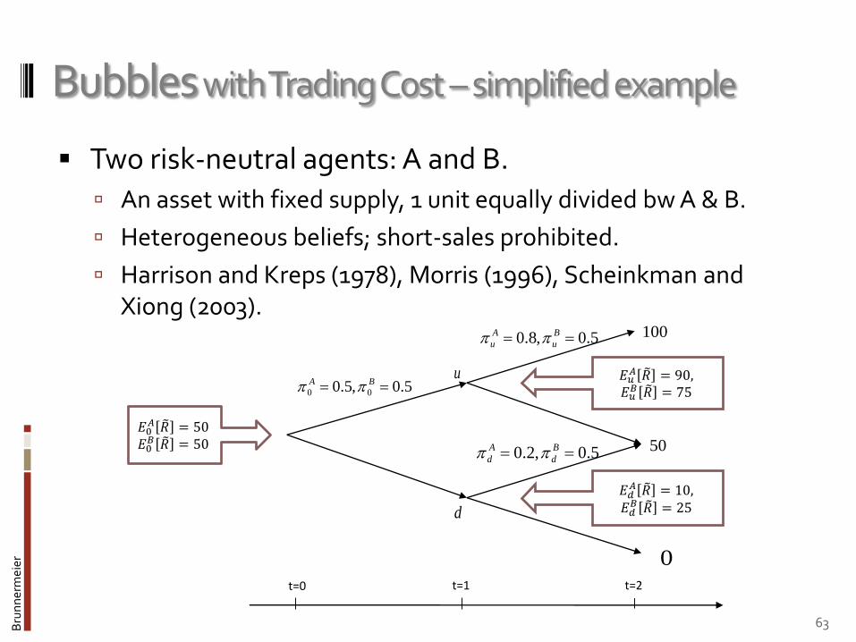
Two risk-neutral agents: A and B.
An asset with fixed supply, 1 unit equally divided bw A & B.
Heterogeneous beliefs; short-sales prohibited.
Harrison and Kreps (1978), Morris (1996), Scheinkman and Xiong (2003).
60
t=0 t=1 t=2
u
d
0
5.0,8.0 B
u
A
u
50
100
5.0,2.0 B
d
A
d
5.0,5.0 00 BA

Bru
nn
erm
eier
Bubbleswith Trading Cost – simplified example
Two risk-neutral agents: A and B.
An asset with fixed supply, 1 unit equally divided bw A & B.
Heterogeneous beliefs; short-sales prohibited.
Harrison and Kreps (1978), Morris (1996), Scheinkman and Xiong (2003).
61
t=0 t=1 t=2
u
d
0
5.0,8.0 B
u
A
u
50
100
5.0,2.0 B
d
A
d
5.0,5.0 00 BA 𝐸𝑢𝐴 ෨𝑅 = 90,
𝐸𝑢𝐵 ෨𝑅 = 75

Bru
nn
erm
eier
Bubbleswith Trading Cost – simplified example
Two risk-neutral agents: A and B.
An asset with fixed supply, 1 unit equally divided bw A & B.
Heterogeneous beliefs; short-sales prohibited.
Harrison and Kreps (1978), Morris (1996), Scheinkman and Xiong (2003).
62
t=0 t=1 t=2
u
d
0
5.0,8.0 B
u
A
u
50
100
5.0,2.0 B
d
A
d
5.0,5.0 00 BA 𝐸𝑢𝐴 ෨𝑅 = 90,
𝐸𝑢𝐵 ෨𝑅 = 75
𝐸𝑑𝐴 ෨𝑅 = 10,
𝐸𝑑𝐵 ෨𝑅 = 25
Bru
nn
erm
eier
Bubbleswith Trading Cost – simplified example
Two risk-neutral agents: A and B.
An asset with fixed supply, 1 unit equally divided bw A & B.
Heterogeneous beliefs; short-sales prohibited.
Harrison and Kreps (1978), Morris (1996), Scheinkman and Xiong (2003).
63
t=0 t=1 t=2
u
d
0
5.0,8.0 B
u
A
u
50
100
5.0,2.0 B
d
A
d
5.0,5.0 00 BA 𝐸𝑢𝐴 ෨𝑅 = 90,
𝐸𝑢𝐵 ෨𝑅 = 75
𝐸𝑑𝐴 ෨𝑅 = 10,
𝐸𝑑𝐵 ෨𝑅 = 25
𝐸0𝐴 ෨𝑅 = 50
𝐸0𝐵 ෨𝑅 = 50

Bru
nn
erm
eier
Bubbleswith Trading Cost – simplified example
Two risk-neutral agents: A and B.
An asset with fixed supply, 1 unit equally divided bw A & B.
Heterogeneous beliefs; short-sales prohibited.
Harrison and Kreps (1978), Morris (1996), Scheinkman and Xiong (2003).
64
t=0 t=1 t=2
u
d
0
5.0,8.0 B
u
A
u
50
100
5.0,2.0 B
d
A
d
5.0,5.0 00 BA 𝐸𝑢𝐴 ෨𝑅 = 90,
𝐸𝑢𝐵 ෨𝑅 = 75
𝐸𝑑𝐴 ෨𝑅 = 10,
𝐸𝑑𝐵 ෨𝑅 = 25
𝐸0𝐴 ෨𝑅 = 50
𝐸0𝐵 ෨𝑅 = 50
𝑝𝑢 = 90
𝑝𝑑 = 25
Bru
nn
erm
eier
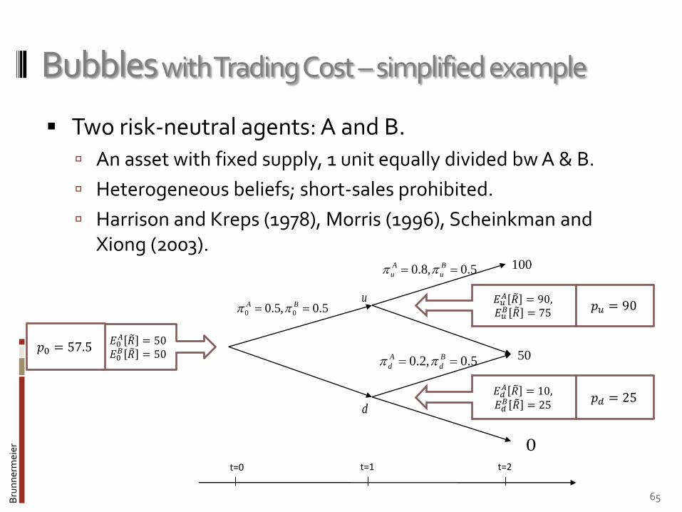
Bubbleswith Trading Cost – simplified example
Two risk-neutral agents: A and B.
An asset with fixed supply, 1 unit equally divided bw A & B.
Heterogeneous beliefs; short-sales prohibited.
Harrison and Kreps (1978), Morris (1996), Scheinkman and Xiong (2003).
65
t=0 t=1 t=2
u
d
0
5.0,8.0 B
u
A
u
50
100
5.0,2.0 B
d
A
d
5.0,5.0 00 BA 𝐸𝑢𝐴 ෨𝑅 = 90,
𝐸𝑢𝐵 ෨𝑅 = 75
𝐸𝑑𝐴 ෨𝑅 = 10,
𝐸𝑑𝐵 ෨𝑅 = 25
𝐸0𝐴 ෨𝑅 = 50
𝐸0𝐵 ෨𝑅 = 50
𝑝𝑢 = 90
𝑝𝑑 = 25
𝑝0 = 57.5

Bru
nn
erm
eier
Welfare criterions heterogeneous beliefs
Given a social welfare function W, allocation 𝑥 ≽𝑊 𝑥′ if
𝐸𝐴 𝑊 𝑢𝐴 𝑥 , 𝑢𝐵 𝑥 ≥ 𝐸𝐴 𝑊 𝑢𝐴 𝑥′ , 𝑢𝐵 𝑥′ AND
𝐸𝐵 𝑊 𝑢𝐴 𝑥 , 𝑢𝐵 𝑥 ≥ 𝐸𝐵 𝑊 𝑢𝐴 𝑥′ , 𝑢𝐵 𝑥′
Back to Bubble example Assume linear and symmetric social welfare function:
𝑊 𝑢𝐴, 𝑢𝐵 = 𝑢 𝑐𝐴 + 𝑢 𝑐𝐵 = 𝑐𝐴 + 𝑐𝐵. At the status quo:
𝐸0𝑗[𝑊(𝑢𝐴, 𝑢𝐵)] = 𝐸0
𝑗[ ෨𝑅] = 50, ∀𝑗 ∈ {𝐴, 𝐵}.
Suppose that trading costs 𝑘 per share. 𝑘 < 15 so that trading occurs.
In the equilibrium:
𝐸0𝑗𝑊 𝑢𝐴, 𝑢𝐵 = 𝐸0
𝑗 ෨𝑅 −𝑘
2= 50 −
𝑘
2, ∀𝑗 ∈ {𝐴, 𝐵}.
66
Brunnermeier & Xiong 2011