UNIVERSITY OF LJUBLJANAFACULTY OF MATHEMATICS AND PHYSICS

DEPARTMENT OF PHYSICS

Princeton Ocean Model

Seminar

Abstract

Princeton Ocean Model, usually called POM was developed by George Mellor and AlanBlumberg around 1977. The model was developed and applied to oceanographic problemsat Princeton University. The model is under GNU license and it can be downloaded fromhttp://www.aos.princeton.edu/WWWPUBLIC/htdocs.pom/. POM was applied to manyocean forecasting systems, which predict hurricanes, tsunamis, ocean currents and oceanwaves. POM uses Arakawa C-grid and central difference LEAP-FROG scheme.

Advisor: Author:

dr. Vlado Malacic Gasper Stifter

Ljubljana, May, 2007

Contents

1 Introduction 3

1.1 Global ocean models . . . . . . . . . . . . . . . . . . . . . . . . . . . . . . . . . 31.2 Coastal models . . . . . . . . . . . . . . . . . . . . . . . . . . . . . . . . . . . . 41.3 Important concepts . . . . . . . . . . . . . . . . . . . . . . . . . . . . . . . . . . 4

2 The Princeton Ocean Model 5

3 Basic equations 6

3.1 Dynamic and Thermodynamic Equations . . . . . . . . . . . . . . . . . . . . . . 7

4 Finite difference scheme 8

4.1 One dimensional case - Forward difference . . . . . . . . . . . . . . . . . . . . . 84.2 One dimensional case - Central difference . . . . . . . . . . . . . . . . . . . . . . 84.3 LEAP - FROG scheme . . . . . . . . . . . . . . . . . . . . . . . . . . . . . . . . 9

5 Boundary conditions 10

6 Sigma coordinate system 11

7 Seamount problem 12

8 Adriatic Tsunami simulation 16

9 Conclusion 17

List of Figures

1 Forward Difference(solid line) and central-difference (dashed line) . . . . . . . . 92 Arrangement of points for computation in leap-frog method . . . . . . . . . . . 103 The sigma coordinate system . . . . . . . . . . . . . . . . . . . . . . . . . . . . 114 Seamount bottom topography, legend shows depth in meters . . . . . . . . . . . 125 Surface flux and surface elevation, legend shows surface elevation in meters . . . 136 Locations of current profiles . . . . . . . . . . . . . . . . . . . . . . . . . . . . . 147 Velocity profiles in points A, B, C in figure 6 . . . . . . . . . . . . . . . . . . . . 148 Velocity u - X section . . . . . . . . . . . . . . . . . . . . . . . . . . . . . . . . . 159 Adriatic Tsunami[6] . . . . . . . . . . . . . . . . . . . . . . . . . . . . . . . . . . 17

2

1 Introduction

Numerical models[1] of ocean currents have simulate flows in realistic ocean basins with a real-istic sea-floor. They include the influence of viscosity and non-linear dynamics and with themone can calculate and also predict flows in the ocean. Perhaps the most important, they in-terpolate between sparse observations of the ocean collected by ships, drifters, and satellites.Numerical models are not absolutely accurate and could never give complete descriptions of theoceanic flows even if the equations are integrated accurately. Models use algebraic approxima-tions of the differential equations. We assume the ocean basins are filled with a grid of pointsand time moves forward in tiny steps. The values of the current, pressure, temperature, andsalinity are calculated from their values at neighbouring points and values from the previoustime. Another limitation of numerical models is that they do provide information only at gridpoints, the results don’t give information about the flow between the grid points. Yet, theocean is turbulent and any oceanic model capable of resolving the turbulence needs grid pointsspaced millimeters apart, with time steps of milliseconds. Practical ocean models have gridpoints spaced tens to hundreds of kilometers apart in horizontal direction and tens to hundredsof meters apart in the vertical. That means the turbulence cannot be calculated directly andthe influence of turbulence must be parametrized. Models of the ocean must run on currentavailable computers, which have limited resources, that means oceanographers have to simplifytheir models further, if they want to finish calculation in decent time. Oceanographers usethe hydrostatic and Boussinesq approximations and often use vertically integrated equations,called the shallow-water equations. It is necessary to do the simplification of the real problem,because we currently unable to run the most detailed models of oceanic circulation for thetime period of thousands of years to understand the role of the ocean in climate[7]. Numericalmodels are used for many purposes in oceanography in general we can divide models into twogroups:

• Mechanistic models are simplified models used for studying processes. Because themodels are simplified, the output is easier to interpret than output from more complexmodels. Many different types of simplified models have been developed, including modelsfor describing planetary waves, the interaction of the flow with sea-floor or the responseof the upper ocean to the wind. These are perhaps the most useful models, because theyprovide insight into the physical mechanisms influencing the ocean.

• Simulation models are used for calculating realistic circulation of oceanic regions. Themodels are often very complex because all important processes are included and theoutput is difficult to interpret. The first simulation models were developed by Kirk Bryanand Michael Cox at the Geophysical Fluid Dynamics laboratory at Princeton.

1.1 Global ocean models

Several types of global models are widely used in oceanography[1]. Most have grid pointsabout one tenth of a degree apart, which is sufficient to resolve mesoscale eddies. Geophysical

Fluid Dynamics Laboratory Modular Ocean Model MOM is perhaps the most widely

3

used model growing out of the original Bryan-Cox code. The model uses the momentumequations, equation of state, and the hydrostatic and Boussinesq approximations. Subgrid–scale motions are reduced by use of eddy viscosity, which neglects small–scale vortices (oreddies). Global ocean models have an implementation of improved numerical schemes, a freesurface, realistic bottom features and many types of mixing including horizontal mixing alongsurfaces of constant density and can be coupled to atmospheric models. Hybrid Coordinate

Ocean Model HYCOM, which is a Global ocean model, have implementation of real x, y, zcoordinates. That type of Cartesian coordinate system has both advantages and disadvantages.It has high resolution in the surface mixed layers and also in shallower regions, but it is lessuseful in the interior of the ocean. Below the mixed layer, mixing in the ocean is easily calculatedalong surfaces of constant density, but difficult across the same surfaces.

1.2 Coastal models

The great economic importance of the coastal zone has led to the development of many differentnumerical models for describing coastal currents, tides, and storm surges. The models extendfrom the beach to the continental slope and they can include a free surface, realistic coasts andbottom features, river runoff and atmospheric forcing. Because the models don’t extend veryfar into deep water, they need additional information about deep–water currents or conditionsat the shelf break. Princeton Ocean Model developed by Blumberg and Mellor (1987)[5]is widely used for describing coastal currents. It is a direct descendant of the Bryan-Coxmodel. It includes thermodynamic processes, turbulent mixing, Boussinesq and hydrostaticapproximations. The model has been used for calculation of results, presented in this seminar,it has been used for calculation of the three–dimensional velocity distribution, salinity, sea level,temperature and turbulence for up to 30 days, over a region roughly 100-1000km on a side withgrid spacing of 1-50km, some of those results are presented in this document, the basin in thisexample was a rectangular basin with an underwater island in the middle of basin.

1.3 Important concepts

• Numerical models are used to simulate oceanic flows with realistic and useful results.The most recent models include heat fluxes through the surface, wind forcing, mesoscaleeddies, realistic coasts and sea-floor features, and more than 20 levels in vertical.

• Recent models are nowadays quite good, with resolution near 0.1o and has showed previ-ously unknown aspects of the ocean circulation.

• Numerical models are still not perfect. They solve discrete equations, which are not asaccurate as the analytical equations of motion.

• Numerical models cannot reproduce all turbulence of the ocean, because the grid pointsare tens to hundreds of kilometers apart. The influence of turbulent motion over smallerdistances must be calculated from theory and this introduces errors.

4

• Numerical models can be forced by real–time oceanographic data, received from shipsand satellites, to produce forecasts of oceanic variables.

2 The Princeton Ocean Model

The Princeton Ocean Model[8] (POM) is a community general circulation numerical oceanmodel, that can be used to simulate and predict oceanic currents, temperatures, salinity andother water properties. The model code was originally developed in late 1970’s at PrincetonUniversity[4] and Analysis of Princeton[7] by Alan Blumberg and George Mellor with latercontributions from other people. The model incorporates the Mellor-Yamada turbulence schemedeveloped in the early 1970’s by George Mellor and Ted Yamada; this turbulence sub–modelis widely used by oceanic and atmospheric models. In the past, early computer ocean modelssuch as the Bryan-Cox model (developed in the late 1960’s at the Geophysical Fluid DynamicsLaboratory, GFDL, later became the Modular Ocean Model1, MOM)), which aimed mostly atcoarse–resolution simulations of the large–scale ocean circulation, so there was still a need for anumerical model, that can handle high–resolution calculation of coastal ocean. The Blumberg-Mellor[8] model, which later became known as POM, thus included new features, such as freesurface to handle tides, sigma vertical coordinates (i.e., terrain-following) to handle complextopographies and shallow regions, a curvilinear grid, to better handle coastlines and a turbulencescheme to handle vertical mixing. At the early 1980’s, the model was used primarily to simulateestuaries, such as the Hudson-Raritan Estuary (by Leo Oey) and the Delaware Bay (BorisGalperin), but also first attempts to use a sigma coordinate model, for basin-scale problemswhich were simulated with the coarse resolution model of the Gulf of Mexico (Blumberg andMellor) and models of the Arctic Ocean (with the inclusion of ice-ocean coupling by LakshmiKantha and Sirpa Hakkinen). The principal attributes of the POM model are as follows:

• It contains an embedded second moment turbulence closure sub-model to provide verticalmixing coefficients.

• It is a sigma coordinate model in that the vertical coordinate is scaled on the watercolumn depth.

• The horizontal curvilinear orthogonal coordinates and an Arakava C differencing scheme.

• The horizontal time differencing is explicit whereas the vertical differencing is implicit.This later eliminates time constraints for the vertical coordinate and permits the use offine vertical resolution in the surface and bottom boundary layers.

• The model is able to use free surface and a split time step. The external model portionof the model is two–dimensional and uses a short time step based on the CFL2 conditionand the external wave speed. The internal mode is three–dimensional and uses a longtime step based on the CFL condition and the internal wave speed.

1http://www.gfdl.gov/~smg/MOM/MOM.html2CourantFriedrichsLewy condition (CFL condition) is a necessary condition for convergence while solving

certain partial differential equations

5

• Complete thermodynamics have been implemented.

The turbulence closure sub-model is one that was introduced my George Mellor, 1973 and wassignificantly advanced in collaboration with Tetsuji Yamada (Mellor and Yamada, 1974; Mellorand Yamada, 1982). It is often cited in the literature as the Mellor and Yamada turbulenceclosure model. There are other versions of model in existence such as a non-Boussinesq3 versionand a more general vertical coordinate version of which the sigma coordinate is a special case.

3 Basic equations

Here we consider how Newton’s Second Law of Motion can be written in a form, which can beapplied in oceanography:

~F = m~a (1)

It is convenient to write ~a =~Fm

and think of the Law as acceleration, due to the resultant forceacting per unit mass. Resultant force is sum of all forces and is dependent of pressure, gravity,frictional and tidal force. In Cartesian coordinates, with the approximation of hydrostaticsand f-plane4 approximation, the system of equations for free surface liquid, notation has thefollowing vector form:

d~V

dt= −α · ∇p − 2~Ω × ~V + ~g + ~F , (2)

where p is pressure, 2~Ω × ~V is Coriolis therm, ~g is gravity and ~F are other forces includingviscosity. Capital letter V denotes macroscopic – verticaly integreated velocity. Small lettersu, v are x and y component of microscopic–local flow velocity, w denotes microscopic veritalvelocity. Equations can be written also as three component equations:

x : ρ(

dudt

+ f∗w − fv)

= −∂p

∂x+

∂τxx

∂x+

∂τxy

∂y+

∂τxz

∂z(3)

y : ρ(

dvdt

+ fu)

= −∂p

∂y+

∂τxy

∂x+

∂τ yy

∂y+

∂τ yz

∂z(4)

z : ρ(

dwdt

− fu)

= −∂p

∂z− ρg +

∂τxz

∂x+

∂τ yz

∂y+

∂τ zz

∂z, (5)

where f = 2Ω sin ϕ is Coriolis parameter, f∗ = 2Ω cos ϕ is reciprotial Coriolis parameter andeffects the equations only near the equator, in most cases is neglected. Ω is angular velocityaround Earth’s axis, ϕ defines position on the Erath’s surface in north-south direction. Equa-tions are written as three component equation, with the coordinates x, y, z and their respectivevelocity components u, v and w, being positive in the east, north and upward directions re-spectively. The origin of coordinates being at the sea surface, ρ is density of sea watter, τ isfriction tensor and g is gravity.

3Density differences are neglected unless differences are multiplied by gravity.4The f-plane approximation is an approximation where the Coriolis parameter, f, is set to a constant value.

6

3.1 Dynamic and Thermodynamic Equations

For simplifying the problem, two approximations are used[8]. Firstly, it is assumed that theweight of the fluid identically ballances the pressure (hydrostatic assumption) and secondly,density differences are neglected unless the differences are multiplied by gravity (Boussinesqueapproximation).Consider a system woth orthogonal Cartesian coordinates, x increasing eastwards, y increasingnorthward and z increasing vertically upwards. The free surface is located at z = η(x, y, t)

and the bottom is at z = −H(x, y). If ~V is horizontal macroscopic–global velocity vector withcomponents and ∇ the horizontal gradient operator, W is macroscopic vertical velocity, thecontinuity equation follows[2]:

∇ · ~V +∂W

∂z= 0. (6)

The Raynolds momentum equations are:

∂U

∂t+ ~V · ∇U + W

∂U

∂z− fV = −

1

ρ0

∂P

∂x+

∂

∂z

(

KM

∂U

∂z

)

+ Fx (7)

∂V

∂t+ ~V · ∇V + W

∂V

∂z+ fU = −

1

ρ0

∂P

∂y+

∂

∂z

(

KM

∂V

∂z

)

+ Fy (8)

ρg = −∂P

∂z, (9)

with ρ0 reference density, ρ density, g gravitational acceleration, P the pressure, KM5 vertical

eddy diffusivity of turbulent momentum mixing. The latitudinal variation of the Coriolis pa-rameter f is introduced by use of β6 plane approximation.The pressure at depth z can be obtained as:

p =∫ η

zρgdz = ρ0gη +

∫ Q

zρgdz = ρ0gη + ps, (10)

where η is deviation of free surface from its undisturbed position Q and the ps is:

ps =∫ Q

zρgdz. (11)

The conservation equations for temperature Θ and salinity S may be written as:

∂Θ

∂t+ ~V · ∇Θ + W

∂Θ

∂z=

∂

∂z

(

KH

∂Θ

∂z

)

+ FΘ (12)

∂S

∂t+ ~V · ∇S + W

∂S

∂z=

∂

∂z

(

KH

∂S

∂z

)

+ FS, (13)

5The turbulent transfer of momentum by eddies giving rise to an internal fluid friction, in a manner analogousto the action of molecular viscosity in laminar flow, but taking place on a much larger scale. The value of thecoefficient of eddy viscosity (an exchange coefficient) is of the order of 1m

2s1, or one hundred thousand times

the molecular kinematic viscosity.6An approximation whereby the Coriolis parameter, f, is set to vary linearly in space is called a beta plane

approximation.

7

where Θ is temperature and S is the salinity. The vertical eddy–macroscopic diffusivity for tur-bolent mixing of heat and salt is denoted as KH . Because the microscopic processes responsiblefor fluid mixing are too complex to model in detail, oceanographers generally treat fluid mixingas a macroscopic ”eddy” diffusion process. Using the temperature and salinity, the density isderived according to an equation of state and has the form:

ρ = ρ (Θ, S) . (14)

The density is ρ, that is, the density evaluated as a function of temperature and salinity, butat atmospheric pressure and it provides accurate density information.

4 Finite difference scheme

A rectangular grid[7] xi, yi, zi is specified and the whole domain is represented as a set of gridboxes. Lateral boundaries coincide with vertical planes passing though the grid nodes. Theupper boundary of the grid boxes changes in time while the lower boundary is fixed, beeingdetermined by the bottom relief. The vertical step varies from surface to the bottom and thenumber of layers is determined by the overall depth and changes from one (when the upperand lower layers coincide) up to n.

4.1 One dimensional case - Forward difference

The most direct method for numerical differentiation of a function starts by expanding it inTaylor series. This series advances the function one small step forward:

f(x + h) = f(x) + hf′

(x)h2

2f

′′

(x) +h3

6f

′′′

(x) + . . . , (15)

where h is the step size. We obtain the forward difference derivate algorithm by solving (5) forf(x):

f′

c ≃f(x + h) − f(x)

h(16)

≃ f′

(x) +h

2f

′′

(x) + . . . , (17)

where the subscript c denotes a computed expression. One can think of this approximation asusing two points to represent the function by a straight line in te interval from x to x +h. Theapproximation has an error proportional to h.

4.2 One dimensional case - Central difference

An improved approximation to the derivative starts with the basic definition (6). Rather thanmaking a single step of h forward, we form central difference by stepping forward by h/2 andbackward by h/2:

f′

c ≈f(x + h/2) − f(x − h/2)

h= Dcf(x, h). (18)

8

Figure 1: Forward Difference(solid line) and central-difference (dashed line)

The important difference from (6) is that when f(x − h/2) is substracted from f(x + h/2), allterms containing an odd power of h in Taylor series disappear. Therefore, the central-differencealgorithm becomes accurate to one order higher in h; that is, h2. If function is well behaved;that is, if (f 3h2)/24 ≪ (f 2h)/2, then one can expect the error by central differrence methodto be smaller than error, produced by the forward difference (6).

4.3 LEAP - FROG scheme

The leap-frog scheme used in POM[9] model described in the present paper is a central differencescheme with trunction error of second order. If we look at the figure 2, the time derivate of ηwould be:

∂η

∂t=

1

∆t

[

ηk+1i,j − ηk

i,j

]

, (19)

where partial derivates of M , N are:

∂M

∂x=

1

∆x

[

Mk+

1

2

i+ 1

2,j− M

k+1

2

i− 1

2,j

]

(20)

∂N

∂y=

1

∆y

[

Nk+

1

2

i,j+ 1

2

− Nk+

1

2

i,j− 1

2

]

. (21)

Indices i,j are grid indices of XY plane on chosen depth, while index k is time step in thisparticular case. An example shown in figure 2 is two–dimensional and the third parameter istime. It is possible to solve shallow watter equations (3-5) in 3D, while the fourth parameter istime, but it is harder to draw and understand the scheme. Because it is easier to understand

9

Figure 2: Arrangement of points for computation in leap-frog method

2D scheme, in this paper it will be only two dimensional grids will be dicoused. Assuming thatvalues at k and k + 1/2 time steps are known, the only unknown η(i, j, k + 1) is derived as:

ηk+1i,j = ηk

i,j −∆t

∆x

[

Mk+

1

2

i+ 1

2,j− M

k+1

2

i− 1

2,j

]

−∆t

∆y

[

Nk+

1

2

i,j+ 1

2

− Nk+

1

2

i,j− 1

2

]

. (22)

As seen in figure 2, values of M , N are specified at the edge of the box, while the result forthe variable η is specified at the center of box. This scheme is known in literature as ArakawaC-grid. All other shallow watter equations (3-5) are similary implemented in the ocean model.

5 Boundary conditions

Wind stress components, kinematics conditions and buoyancy flux were specified at the seasurface as[9]:

Nz

∂u

∂z= τOx, Nz

∂v

∂z= τOy,

∂η

∂t+ u

∂η

∂x+ v

∂η

∂y= w, Kz

∂ρ

∂z= 0, (23)

where τOx and τOy are components of wind stress vector at the surface in x and y directionrespectively. Boundary conditions at the bottom are specified as:

Nz

∂u

∂z= τbx, Nz

∂v

∂z= τby, u

∂H

∂x+ v

∂H

∂y= w, Kz =

∂ρ

∂t= 0, (24)

where τbx and τby are bottom fricition stress written as:

(τbx, τby) =(

αub| ~Ub|, αvb| ~Ub|)

. (25)

10

Ub is current speed near bottom, bottom friction coeficient is choosen as α = 2.5·10−3, α = ρ0Cd,where ρ0 is densitiy and Cd is drag coefficient at barometric pressure, given by:

Cd =[

1

κln (H + zb) /z0

]

−2

. (26)

The bottom stress coefficient is determined by matching velocities with logarithmic law of wall.zb and u, v are grid points and corresponding velocities in the grid point nearest to the bottomand κ is the von Karman constant. The parameter z0 depends on the local bottom roughnessand is typically set for the ocean to z0 = 1cm, as suggested by Weatherly and Martin [1978].Near bottom at the boundary layer, for determining fluid profile kinematic viscosity is used, sothe profile is not turbulent.

6 Sigma coordinate system

To simplify solving basic equations, while bottom topography is included in calculation, itis vise to transform our basic equations(3-5) (shallow watter equations) in sigma coordinatesystem[4]. The new coordinates would be:

x = x∗, y = y∗, σ =z − η(t)

H(x) − η(x, t), (27)

where σ becomes a vertical coordinate in z direction, but it has a value within [0,1]. σ = 0 atthe surface and σ = −1 at the bottom. x, y, t are ordinary Cartesian coordinates. If the basicequations are transformed in sigma coordinates, then the equations are always in same form,which means it is independent of the bottom topography.

Figure 3: The sigma coordinate system

11

7 Seamount problem

In this section we would examine, fluxes, surface elevation on sea-mount case with model basedon Leap-frog scheme. Bottom topography of the sea-mount problem is shown in figure 4:

Figure 4: Seamount bottom topography, legend shows depth in meters

The basin in figure7 4 is 3500 km long and 2500 km wide. In the center bottom rises from−4500 m to −400 m. From west it flows prescribed flux with velocity 0.2m/s. In figure 5 itis shown profile of the flux at 15th of 49 sigma level and surface elevation. In this case basinwas closed in all directions. It is clearly seen, what effect would have bottom topography oncurrents and surface elevation. Coriolis parameter was set to 1−4/s, salinity was neglected,3D calculation was performed with temperature and salinity held fixed, advection scheme wascentred, as originally provided with POM, grid size was 65 × 49 points, there were 49 sigma

7All plots are made with John Hunter’s Pomviz package in Matlab in standard form used in oceanography,the graphs have units which are use as a standard in oceanography, end are derived from the package used inMatlab http://staff.acecrc.org.au/~johunter/ozpom/readme_pomviz

12

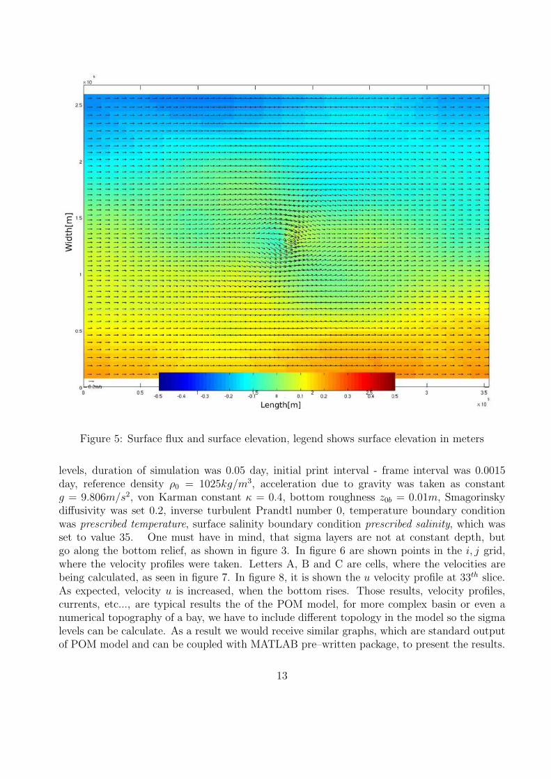
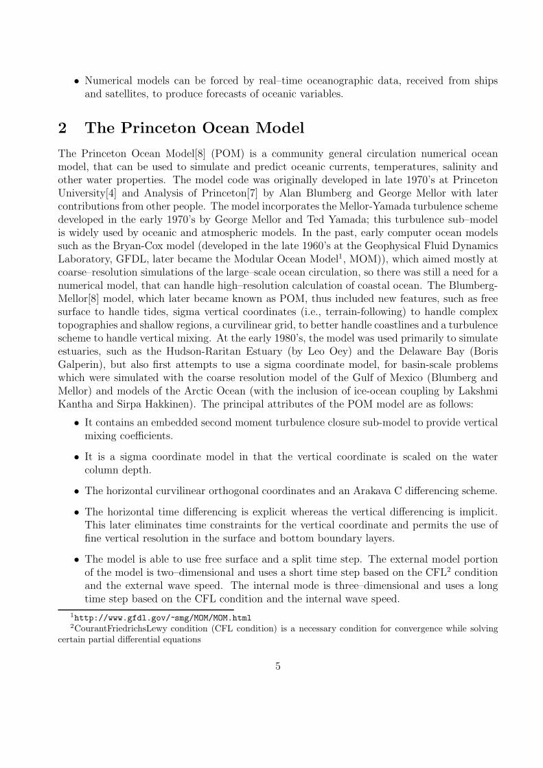
Figure 5: Surface flux and surface elevation, legend shows surface elevation in meters

levels, duration of simulation was 0.05 day, initial print interval - frame interval was 0.0015day, reference density ρ0 = 1025kg/m3, acceleration due to gravity was taken as constantg = 9.806m/s2, von Karman constant κ = 0.4, bottom roughness z0b = 0.01m, Smagorinskydiffusivity was set 0.2, inverse turbulent Prandtl number 0, temperature boundary conditionwas prescribed temperature, surface salinity boundary condition prescribed salinity, which wasset to value 35. One must have in mind, that sigma layers are not at constant depth, butgo along the bottom relief, as shown in figure 3. In figure 6 are shown points in the i, j grid,where the velocity profiles were taken. Letters A, B and C are cells, where the velocities arebeing calculated, as seen in figure 7. In figure 8, it is shown the u velocity profile at 33th slice.As expected, velocity u is increased, when the bottom rises. Those results, velocity profiles,currents, etc..., are typical results the of the POM model, for more complex basin or even anumerical topography of a bay, we have to include different topology in the model so the sigmalevels can be calculate. As a result we would receive similar graphs, which are standard outputof POM model and can be coupled with MATLAB pre–written package, to present the results.

13

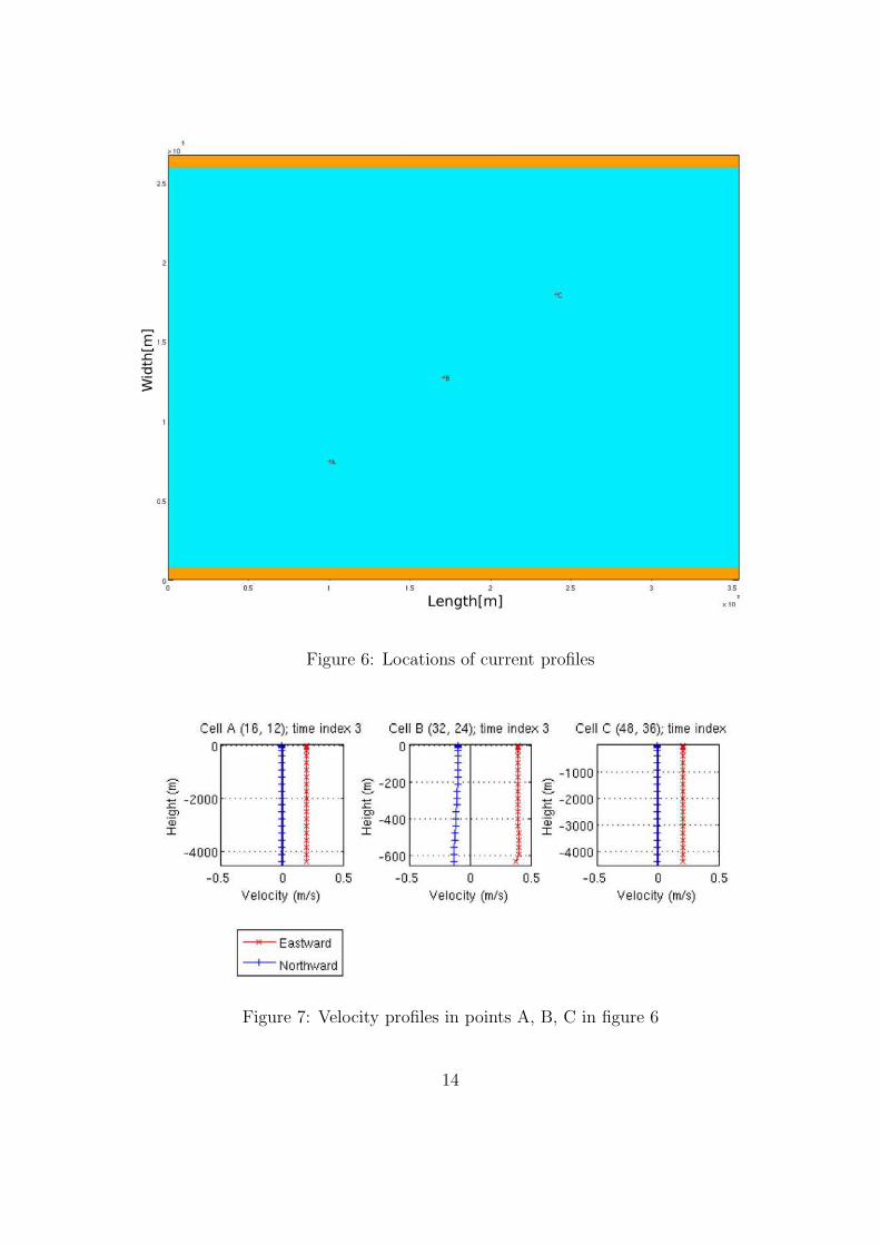
Figure 6: Locations of current profiles

Figure 7: Velocity profiles in points A, B, C in figure 6

14

Figure 8: Velocity u - X section

The units of all graphs are left in scientific number format, because that is the standardizationin oceanography and all visualization tools used in oceanography use that units as standard inoceanography.

15

8 Adriatic Tsunami simulation

Dr. V. Malacic and B. Petelin, M. Sci, have performed a simulation of Adriatic Tsunami[6].They simulated the spread of Tsunami generated by a sub–sea quake near Bar situated in aseismically active region of Montenegro. An earthquake of magnitude 6.8 on the Richter scalewith an epicentre at 13km depth which could generate a wave of 0.25m at the open sea. Forthis simulation the sea level – surface exactly, near Bar was initially perturbed for 10 minutesduration with an oscillation of 0.5 meter amplitude and period of 30 seconds. The simulationwas performed using the 3–dimensional Princeton Ocean Model (POM), which is routinely usedby the MBS (Marine Biology Station in Piran) and by the National Institute for Geophysicsand Volcanology in Bologna, to forecast the circulation of water masses within the Adriatic sea.The POM model had had a spatial grid of 5km x 5km, similar simulations were carried out atthe Geophysics Institute in Zagreb twenty years ago and the results published in the popularjournal Priroda (Ima li Tsunamija u Jadranskom moru, Mirko Orlic, Priroda, May-june,1984,310-311). The POM’s simulation of Tsunami confirmed the earlier results. The wave takesmore than 6 hours to arrive at the Gulf of Trieste with strongly attenuated amplitude of lessthan 0.004m (4 mm). The tsunami attenuates principally due to destructive interference fromwaves that are reflected by coast and by the pronounced bathymetric variations (rising seafloor) in the southern Adriatic basin. The broken region of periodic wave reinforcement dueto constructive interference also experiences destructive interference, with stray reflected wavesand so is not stable. In addition the propagating tsunami loses energy due to wave frictionin the shallow waters of the northern Adriatic. The numerical simulation may overestimatethis friction and it need to be investigated further. However, even with a drastic reduction insimulated friction, the anticipated wave amplitude in the Gulf of Trieste is expected to be lessthan 0.4 m because it must be reduced from the wave amplitude in the generation region nearBar.

16

Figure 9: Adriatic Tsunami[6]

9 Conclusion

Numerical models of ocean circulation are among the most demanding tasks performed bycomputers today. Although some simple models used on small region of the ocean, over a shorttime period, can be solved on a personal computer, realistic global models take thousands ofhours on the fastest super computers available. One way to get this kind of computationalpower is to link many computers together to work on a problem, this strategy is known as”parallel computing”[7]. Much of the numerical work done at COAS utilizes a massively parallelConnection Machine CM5 which consists of 64 fast processors linked together by a fast networkand coordinated by special software. Other modeling work at COAS uses a Silicon GraphicsPower Challenge and an IBM SP2. The computer facilities at COAS are among the finest

17

available at any oceanographic research institution anywhere in the world. Even when thefastest computers are used, numerical models are only approximations of the full dynamics andthermodynamics, the solutions are therefore only approximations. One way to correct errors,caused by algorithm in the model, is to apply a procedure known as ”data assimilation”,which blends the model approximations with observations of the real ocean in a least–squareerror sense. This blending takes into account, the errors produces by the model, dynamicsand thermodynamics, as well as measurement errors made by observations. Princeton Oceanmodel was used for simulating many problems in dynamical oceanography. There are alsomany other ocean models in use, but most widespeaded is the POM, developed by Mellorand Blumberg. All models use similar Arakawa C-grid [8], but there are many differences inroutines for calculating turbulent terms in shallow watter equations. Those routines were notdescribed in this seminar. With faster computers and large clusters it is possible to solvelarger problems on larger, more detailed grid. Most advancing technology uses multi processorhardware and most promising are graphics processors and GPU scientific clusters like NvidiaTesla. Research in physical oceanography is basically divided in two parts, model developing,which is described in this paper and in theoretical physical oceanography. Theoretical physicaloceanographers are trying to describe problems analytically, but unfortunately, nowadays it isstill hard to solve even most simple oceanographic problems analytically, with an exceptionof few examples. That is one reason more, why is research in that field so important. Mostdifficult is to understand the turbulent terms in shallow watter theory and even harder tofind a perfect model for calculation of turbulent term, that is the reason why are so many ofocean models in use. There is no universal model for solving oceanographic problems, we haveto change the model for every particular problem. Ocean models are applied to automaticocean forecasting systems like: Princeton Regional Ocean Forecasting System (GOM), NewYork Harbor Observing and Prediction System (NYHOPS), U.S. Coastal Observing System(COOS) and many others. Most important in our region is Adriatic Sea Forecasts (INGV)in Italy. All those models use as input combination of data measured with ocean stationsand data received from satellites. This field of physics is important for weather prediction andprediction of hurricanes like Catrina in the USA or well known Tsunami, which killed thousandsof people in Indonesia and India few years ago. Physical oceanographers have predicted in everyparticular case possible catastrophe, but the governments in that regions did not react as theyshould have.

18

References

[1] Robert.H.Stewart, Introduction to Physical Oceanography, Department of Oceanography,Texas A&M University http://oceanworld.tamu.edu

[2] M. Bone, Development of a Non-linear Levels Model and its Application to Bora-driven

Circulation on the Adriatic Shelf, p. 475-496, stuarine, Costal and Shelf Science (1993).

[3] S.K.Popov, Density and residual tidal circulation and related mean sea level of the Barents

Sea, IOC Workshop report No. 171, p. 107-129, UNESCO, IOCWorkshop Report No. 171,Annex III, Toulouse, France, 10-11 May 1999.

[4] C. Goto and Y. Ogawa, Tohoku University, Numerical method of tsunami simulation

with leap-frog scheme, Part 1, Chapter 1-2, UNESCO, Intergovermental OceanographicCommision, Manuals and Guides, 1997.

[5] George L. Mellor and Alan F. Blumberg, A three-dimensional, primitive equation, nu-

merical ocean model,Program in Atmospheric and Ocean Sciences, Princeton University,Princeton, NJ 08644-0710

[6] Dr. V.Malacic, B.Petelin, M.sci, Adriatic Tsunamis, http://projects.mbss.org/

tsunami/indexa.html

[7] Rubin H.Landau, Manuel Jose Pares Mejıa, Computational physics, Problem Sloving withComputers, John Wiley&Sons, INC.

[8] Alan F. Blumberg and George L. Mellor, A Discription of a Three-Dimensional Coastal

Ocean Circulation Model Dynalysis of Princeton, Princeton, 1987

[9] http://www.aos.princeton.edu/WWWPUBLIC/htdocs.pom/

19