pricing with constrained supply - the university of …metin/or6377/folios/constrained.pdfe 1 u /~...

Pag

e1

utdallas.edu/~metin

Pricing with Constrained Supply

Outline

Pricing with a Supply Constraint

Opportunity Cost

Variable Pricing

Variable Prices in Practice

Based on Phillips (2005) Chapter 5

Pag

e2

utdallas.edu/~metin

Supply Constraint Examples

1. UTD’s Cohort (full-time) MBA program has 50 spots

2. Eismann Center performance hall has 1563 seats

3. Dallas Cowboys Stadium can accommodate up to 111,000 people

4. Royal Caribbean’s cruise ship Voyager of the Seas departs from Galveston. Passengers: 3114 passengers

Inside Cabins: 618

Outside Cabins: 939

Balcony cabins: 757

Suites: 119

5. Airbus A380 can seat 550 passengers

6. A sit-com lasts 30 mins = for 22 min pure sit-com + 7.5 min advertisement + 0.5 min

accommodates 3 advertisement pods (breaks) of approximately about 6th, 16th and 26th minutes of the show.

• Each pod lasts 150 seconds=2.5 minutes.

• During 150 seconds 8-12 commercials can be shown

7. Yahoo.com has three vertical panels: “My favorites”, “Today-news”, “Advertisements” Advertisements panel can accommodate 1 big and 1 small advertisement

Total advertisement area: 10 cm wide and 10 cm long; it can be split into smaller pieces

Pag

e3

utdallas.edu/~metin

Supply Constraint: 𝒃

Constrained pricing problem is

0

)(

))(( max

p

bpdst

cppd(p)

d(p)

p

1. Unconstrained

price solution

2. Demand withunconstrained

solutionCapacityconstraint

b

d(p)

p

Capacityconstraint

b3. Sell entire

capacity

4. Constrained

price solution

p=d-1(b)

?))(( isWhat

.)( then )( If

.price todemand maps (.)

.demand toprice maps (.)

1

1

1

bdd

m

bDbdmpDpd

d

d

Pag

e4

utdallas.edu/~metin

Examples of Constrained Supply

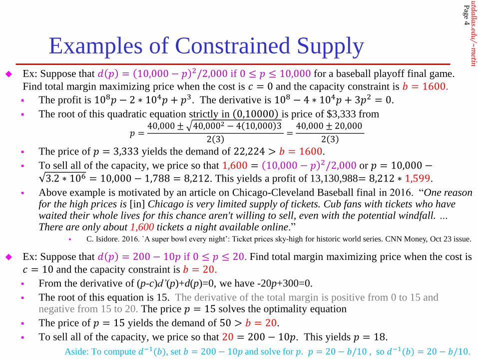
Ex: Suppose that 𝑑 𝑝 = 200 − 10𝑝 if 0 ≤ 𝑝 ≤ 20. Find total margin maximizing price when the cost is

𝑐 = 10 and the capacity constraint is 𝑏 = 20.

From the derivative of (p-c)d’(p)+d(p)=0, we have -20p+300=0.

The root of this equation is 15. The derivative of the total margin is positive from 0 to 15 and negative from 15 to 20. The price 𝑝 = 15 solves the optimality equation

The price of 𝑝 = 15 yields the demand of 50 > 𝑏 = 20.

To sell all of the capacity, we price so that 20 = 200 − 10𝑝. This yields 𝑝 = 18.

Aside: To compute 𝑑−1(𝑏), set 𝑏 = 200 − 10𝑝 and solve for 𝑝. 𝑝 = 20 − 𝑏/10 , so 𝑑−1(𝑏) = 20 − 𝑏/10.

Ex: Suppose that 𝑑 𝑝 = 10,000 − 𝑝 2/2,000 if 0 ≤ 𝑝 ≤ 10,000 for a baseball playoff final game.

Find total margin maximizing price when the cost is 𝑐 = 0 and the capacity constraint is 𝑏 = 1600.

The profit is 108𝑝 − 2 ∗ 104𝑝 + 𝑝3. The derivative is 108 − 4 ∗ 104𝑝 + 3𝑝2 = 0.

The root of this quadratic equation strictly in 0,10000 is price of $3,333 from

𝑝 =40,000 ± 40,0002 − 4 10,000 3

2 3=40,000 ± 20,000

2 3

The price of 𝑝 = 3,333 yields the demand of 22,224 > 𝑏 = 1600.

To sell all of the capacity, we price so that 1,600 = 10,000 − 𝑝 2/2,000 or 𝑝 = 10,000 −3.2 ∗ 106 = 10,000 − 1,788 = 8,212. This yields a profit of 13,130,988= 8,212 ∗ 1,599.

Above example is motivated by an article on Chicago-Cleveland Baseball final in 2016. “One reason for the high prices is [in] Chicago is very limited supply of tickets. Cub fans with tickets who have waited their whole lives for this chance aren't willing to sell, even with the potential windfall. … There are only about 1,600 tickets a night available online.”

C. Isidore. 2016. `A super bowl every night’: Ticket prices sky-high for historic world series. CNN Money, Oct 23 issue.

Pag

e5

utdallas.edu/~metin

Opportunity Cost: Going from 20 to 40

With constraint b, we find

}0 ,)( :))(({max)( pbpdcppdb

)20()40( bb

Under b=20 in the last example, we obtain a profit of (18-10)(20)=160.

Under b=40, we still have that the demand of 50 with p=15 violates the capacity.

We solve for p=d-1(b=40)=20-b/10=16.

The profit then is (16-10)(40)=240.

Opportunity cost of having the capacity of 20 as opposed to 40 is 80:

).20()40(16024080 bb

The benefit of more capacity, say by going from b=20 to b=40, is

Pag

e6

utdallas.edu/~metin

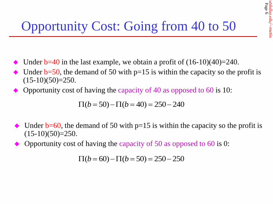
Opportunity Cost: Going from 40 to 50

Under b=40 in the last example, we obtain a profit of (16-10)(40)=240.

Under b=50, the demand of 50 with p=15 is within the capacity so the profit is (15-10)(50)=250.


240250)40()50( bb

Under b=60, the demand of 50 with p=15 is within the capacity so the profit is (15-10)(50)=250.


250250)50()60( bb

Pag

e7

utdallas.edu/~metin

Putting Various Capacities Together

Opportunity Cost

.250)60( );250)50( ;240)40( ;160)20( ;0)0( bbbbb

The profit curve between the pairs of (capacity, profit) that we have evaluated above is not linear. So the profit is drawn in dots.

Because of nonlinearity, marginal opportunity cost is not constant.

b20 40 6050

250

160

Π(𝑏)

Pag

e8

utdallas.edu/~metin

Linear Demand Curve

Marginal Opportunity Cost

Marginal opportunity cost of the capacity is zero when the capacity is more than the demand under the price p0.

Suppose that the demand curve is linear: d(p)=D-mp.

The unconstrained price p0 that maximizes profit is found from the derivative of П(p)=(p-c) (D-mp). The derivative is

.22

)(

is price under this demand The

.2

yields which 02

0

0

mcD

m

mcDmDpd

m

mcDp

mpmcD

)(for 0)(d

d0pdbb

b

See the opportunity cost in the last example for capacity higher than 50.

Pag

e9

utdallas.edu/~metin

Linear Demand CurveMarginal Opportunity Cost with Insufficient Capacity

Suppose that the capacity is insufficient so b<d(p0).

Set the price equal to 𝑑−1(𝑏) to sell the entire capacity.

The marginal opportunity cost is

.continuous iscost marginal theso ,0)(d

dcheck exercisean As

2

b d

d

so /)()( curve demandlinear for ))((d

d)(

d

d

)(

11

0

pdb

bb

m

bc

m

D

cm

b

m

D

b

mbDbdcbdbb

bb

When b=d(p0), b=(D-mc)/2.

Pag

e10

utdallas.edu/~metin

Example: Linear Demand Curve

Marginal Opportunity Cost

Suppose that the demand is linear d(p)=D-mp=200-10p and c=10.

We already computed p0=15 and d(p0)=50.

Then the marginal opportunity cost is

.0)(d

d

.50bfor 5

1010

210

10

2002 )(

d

d

50

b

bb

bb

m

bc

m

Db

b

50 b

10

)(d

db

b

Pag

e11

utdallas.edu/~metin

Summary of Pricing a Single Product

under Capacity Constraint

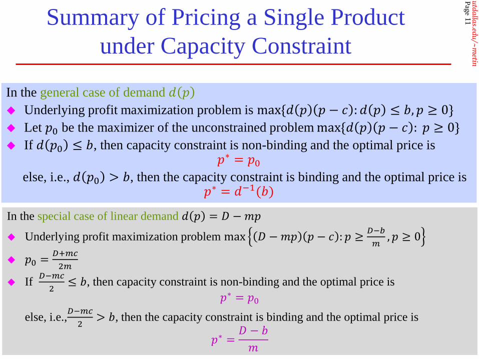
In the general case of demand 𝑑 𝑝

Underlying profit maximization problem is max{𝑑 𝑝 𝑝 − 𝑐 : 𝑑 𝑝 ≤ 𝑏, 𝑝 ≥ 0}

Let 𝑝0 be the maximizer of the unconstrained problem max{𝑑 𝑝 𝑝 − 𝑐 : 𝑝 ≥ 0}

If 𝑑 𝑝0 ≤ 𝑏, then capacity constraint is non-binding and the optimal price is𝑝∗ = 𝑝0

else, i.e., 𝑑 𝑝0 > 𝑏, then the capacity constraint is binding and the optimal price is𝑝∗ = 𝑑−1(𝑏)

In the special case of linear demand 𝑑 𝑝 = 𝐷 −𝑚𝑝

Underlying profit maximization problem max 𝐷 −𝑚𝑝 𝑝 − 𝑐 : 𝑝 ≥𝐷−𝑏

𝑚, 𝑝 ≥ 0

𝑝0 =𝐷+𝑚𝑐

2𝑚

If 𝐷−𝑚𝑐

2≤ 𝑏, then capacity constraint is non-binding and the optimal price is

𝑝∗ = 𝑝0

else, i.e.,𝐷−𝑚𝑐

2> 𝑏, then the capacity constraint is binding and the optimal price is

𝑝∗ =𝐷 − 𝑏

𝑚

Pag

e12

utdallas.edu/~metin

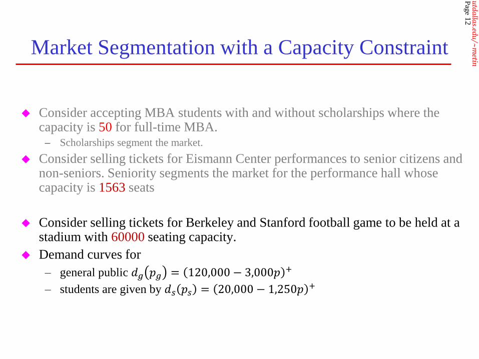
Market Segmentation with a Capacity Constraint

Consider accepting MBA students with and without scholarships where the capacity is 50 for full-time MBA.

– Scholarships segment the market.

Consider selling tickets for Eismann Center performances to senior citizens and non-seniors. Seniority segments the market for the performance hall whose capacity is 1563 seats

Consider selling tickets for Berkeley and Stanford football game to be held at a stadium with 60000 seating capacity.

Demand curves for

– general public 𝑑𝑔 𝑝𝑔 = 120,000 − 3,000𝑝 +

– students are given by 𝑑𝑠 𝑝𝑠 = 20,000 − 1,250𝑝 +

Pag

e13

utdallas.edu/~metin


Single Price

When a single price is charged to both general and student attendees, we have

16. and 20 are solutions becan that prices feasibleonly The

16 if 2500200006000-120000

4016 if 6000-120000

40 if 0

)(

is derivative whose,)250,1000,20()000,3000,120()(

'

pp

ppp

pp

p

pR

pppppR

Since the stadium is sold out at the price of $20, the optimal price is $20.

The optimal revenue under single-price is 20(60,000)=1,200,000.

For 16 < 0 ≤ 40, the candidate for optimal is 𝑝 =120,000

6,000= 20.

For 𝑝 ≤ 16, the candidate for optimal is 𝑝 =140,000

8,500= 16.47 > 16. So 𝑝 = 16.

Pag

e14

utdallas.edu/~metin


Formulation with Multiple Prices

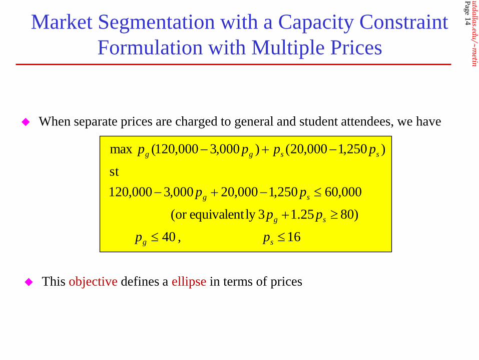
When separate prices are charged to general and student attendees, we have

16 , 40

)8025.13ly equivalentor (

000,60250,1000,20000,3000,120

st

)250,1000,20()000,3000,120( max

sg

sg

sg

ssgg

pp

pp

pp

pppp

This objective defines a ellipse in terms of prices

Pag

e15

utdallas.edu/~metin


Graphical Depiction with Multiple Prices

40

8

16

ps

pg20 80/3

Feasible

Price

Region

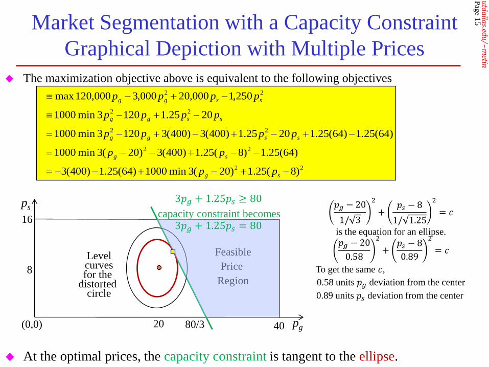
At the optimal prices, the capacity constraint is tangent to the ellipse.

Levelcurvesfor the

distorted circle

(0,0)

The maximization objective above is equivalent to the following objectives

22

22

22

22

22

)8(25.1)20(3 min 1000)64(25.1)400(3

)64(25.1)8(25.1)400(3)20(3 min 1000

)64(25.1)64(25.12025.1)400(3)400(31203min 1000

2025.11203min 1000

250,1000,20000,3000,120 max

sg

sg

ssgg

ssgg

ssgg

pp

pp

pppp

pppp

pppp

𝑝𝑔 − 20

1/ 3

2

+𝑝𝑠 − 8

1/ 1.25

2

= 𝑐

is the equation for an ellipse.

𝑝𝑔 − 20

0.58

2

+𝑝𝑠 − 8

0.89

2

= 𝑐

To get the same 𝑐,

0.58 units 𝑝𝑔 deviation from the center

0.89 units 𝑝𝑠 deviation from the center

3𝑝𝑔 + 1.25𝑝𝑠 ≥ 80

capacity constraint becomes3𝑝𝑔 + 1.25𝑝𝑠 = 80

Pag

e16

utdallas.edu/~metin

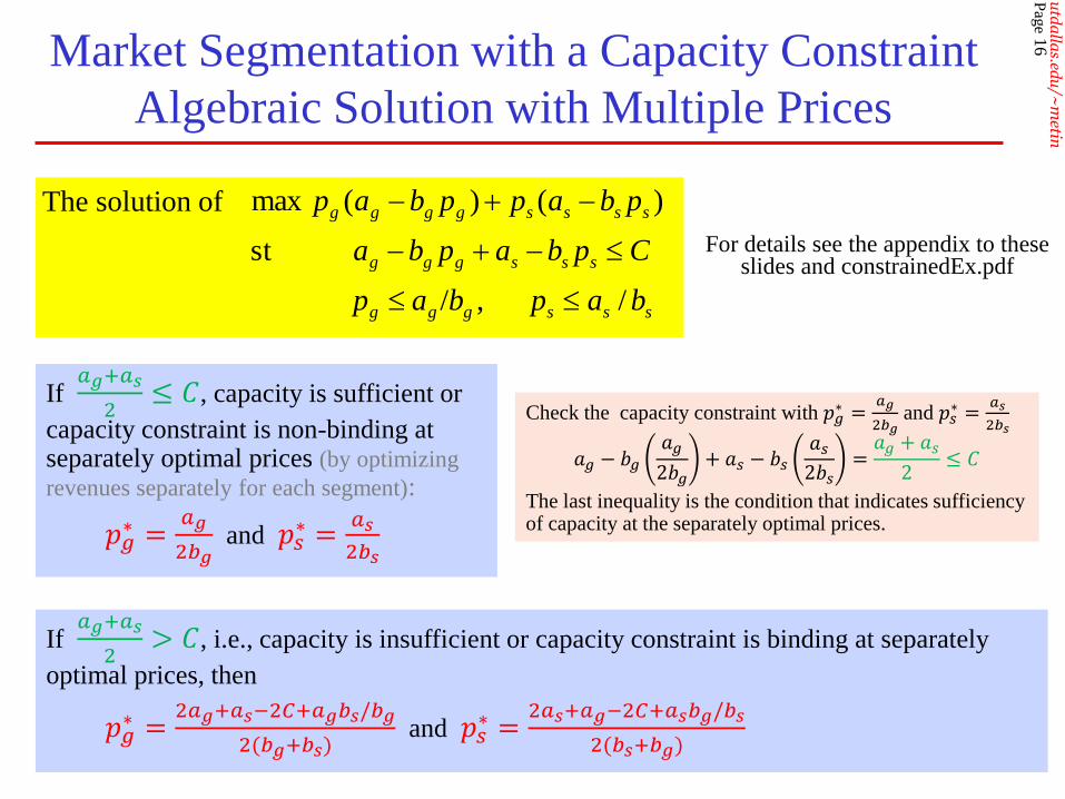
If 𝑎𝑔+𝑎𝑠

2≤ 𝐶, capacity is sufficient or

capacity constraint is non-binding at separately optimal prices (by optimizing

revenues separately for each segment):

𝑝𝑔∗ =

𝑎𝑔

2𝑏𝑔and 𝑝𝑠

∗ =𝑎𝑠

2𝑏𝑠


Algebraic Solution with Multiple Prices

The solution of

sssggg

sssggg

ssssgggg

bapbap

Cpbapba

pbappbap

/ ,/

st

)()( max

For details see the appendix to these slides and constrainedEx.pdf

Check the capacity constraint with 𝑝𝑔∗ =

𝑎𝑔

2𝑏𝑔and 𝑝𝑠

∗ =𝑎𝑠

2𝑏𝑠

𝑎𝑔 − 𝑏𝑔𝑎𝑔

2𝑏𝑔+ 𝑎𝑠 − 𝑏𝑠

𝑎𝑠2𝑏𝑠

=𝑎𝑔 + 𝑎𝑠

2≤ 𝐶

The last inequality is the condition that indicates sufficiency of capacity at the separately optimal prices.


2> 𝐶, i.e., capacity is insufficient or capacity constraint is binding at separately

optimal prices, then

𝑝𝑔∗ =

2𝑎𝑔+𝑎𝑠−2𝐶+𝑎𝑔𝑏𝑠/𝑏𝑔

2(𝑏𝑔+𝑏𝑠)and 𝑝𝑠

∗ =2𝑎𝑠+𝑎𝑔−2𝐶+𝑎𝑠𝑏𝑔/𝑏𝑠

2(𝑏𝑠+𝑏𝑔)

Pag

e17

utdallas.edu/~metin

Market Segmentation with a Capacity ConstraintAlgebraic Solution of an Insufficient Capacity Instance

The solution of

16 , 40

000,60250,1000,20000,3000,120st

)250,1000,20()000,3000,120( max

sg

sg

ssgg

pp

pp

pppp

Check the capacity constraint with 𝑝𝑔∗ = 22.352941 and 𝑝𝑠

∗ = 10.352941

120,000 − 3,000 22.352941 = 52,941.1765 tickets to general public

20,000 − 1,250 10.352941 = 7,058.8235 tickets to students

Capacity constraint is binding : 60,000 tickets to both

The corresponding revenue is $1,256,471; 4.7% more than the revenue under single price.


2=

120+20

2> 60 = 𝐶, i.e., capacity is insufficient or capacity constraint is binding at

separately optimal prices, then

𝑝𝑔∗ =

2𝑎𝑔+𝑎𝑠−2𝐶+𝑎𝑔𝑏𝑠/𝑏𝑔

2(𝑏𝑔+𝑏𝑠)=

2 120 +20−2 60 +120(1.25)/3

2 3+1.25=

190

8.5= 22.352941 and

𝑝𝑠∗ =

2𝑎𝑠+𝑎𝑔−2𝐶+𝑎𝑠𝑏𝑔/𝑏𝑠

2(𝑏𝑠+𝑏𝑔)=

2 20 +120−2 60 +20(3)/1.25

2 1.25+3=

88

8.5=10.352941

The original demand curve for general public: 120,000 − 3,000𝑝𝑔

Pag

e18

utdallas.edu/~metin

Market Segmentation with a Capacity ConstraintAlgebraic Solution of a Sufficient Capacity Instance

The solution of

16 , 30

000,60250,1000,20000,3000,90st

)250,1000,20()000,3000,90( max

sg

sg

ssgg

pp

pp

pppp

Check the capacity constraint with 𝑝𝑔∗ = 15 and 𝑝𝑠

∗ = 8

90,000 − 3,000 15 + 20,000 − 1.25 8 = 45,000 + 10,000

=90,000 + 20,000

2=𝑎𝑔 + 𝑎𝑠

2≤ 𝐶 = 60,000


2=

90+20

2≤ 60 = 𝐶, capacity is sufficient or capacity

constraint is non-binding at separately optimal prices

𝑝𝑔∗ =

𝑎𝑔

2𝑏𝑔=

90

2 3= 15 and 𝑝𝑠

∗ =𝑎𝑠

2𝑏𝑠=

20

2 1.25= 8

The reduced demand curve for general public: 90,000 − 3,000𝑝𝑔

Pag

e19

utdallas.edu/~metin


Continuity of Prices in Capacity

Under insufficient capacity 𝐶 <𝑎𝑔+𝑎𝑠

2, consider increasing capacity and check prices

limC→(𝑎𝑔+𝑎𝑠)/2

𝑝𝑔∗ 𝐶 = lim

C→(𝑎𝑔+𝑎𝑠)/2

2𝑎𝑔+𝑎𝑠−2𝐶+𝑎𝑔𝑏𝑠

𝑏𝑔

2 𝑏𝑔+𝑏𝑠

= limC→(𝑎𝑔+𝑎𝑠)/2

𝑎𝑔 1+𝑏𝑠𝑏𝑔

+𝑎𝑔+𝑎𝑠−2𝐶

2𝑏𝑔 1+𝑏𝑠𝑏𝑔

=𝑎𝑔 1+

𝑏𝑠𝑏𝑔

2𝑏𝑔 1+𝑏𝑠𝑏𝑔

=𝑎𝑔

2𝑏𝑔.

And similarly lim𝐶→(𝑎𝑔+𝑎𝑠)/2

𝑝𝑠∗ 𝐶 =

𝑎𝑠

2𝑏𝑠.

As capacity 𝐶 increases optimal prices decrease towards the separately optimal prices and become separately optimal prices at 𝐶 = (𝑎𝑔 + 𝑎𝑠)/2.

𝑝𝑔∗ 𝐶 =

𝑎𝑔

2𝑏𝑔Slope

𝐶

𝑏𝑔+𝑏𝑠

Insufficient capacity Sufficient capacity

𝐶 =𝑎𝑔 + 𝑎𝑠

2

𝑝𝑠∗ 𝐶 =

𝑎𝑠2𝑏𝑠

Slope 𝐶

𝑏𝑔+𝑏𝑠Insufficient capacity Sufficient capacity

𝐶 =𝑎𝑔 + 𝑎𝑠

2

𝑝𝑔∗ 𝐶 𝑝𝑠

∗ 𝐶

𝐶 𝐶

General Public Prices Student Prices

Pag

e20

utdallas.edu/~metin

Variable Pricing

The prices for

– Theme park tickets vary over a week

– Movie theater rickets vary over a week

– Sport events vary over a season

– Airline tickets vary over a season

– Electricity vary over time of the day

– Phone calls vary over time of the day

– Disney Theme Parks announced investigation of variable pricing in Oct 2015

Pag

e21

utdallas.edu/~metin

Variable Pricing

Single Price

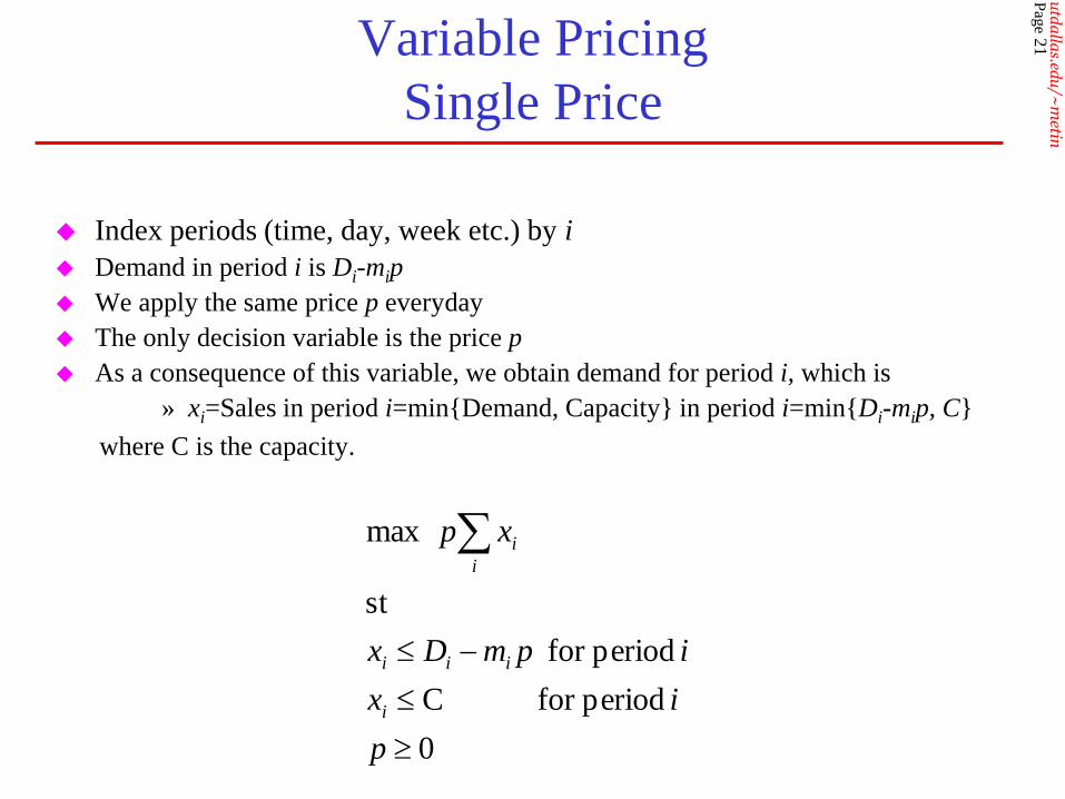
Index periods (time, day, week etc.) by i

Demand in period i is Di-mip

We apply the same price p everyday

The only decision variable is the price p

As a consequence of this variable, we obtain demand for period i, which is

» xi=Sales in period i=min{Demand, Capacity} in period i=min{Di-mip, C}

where C is the capacity.

0

periodfor C

periodfor

st

max

p

ix

ipmDx

xp

i

iii

i

i

Pag

e22

utdallas.edu/~metin

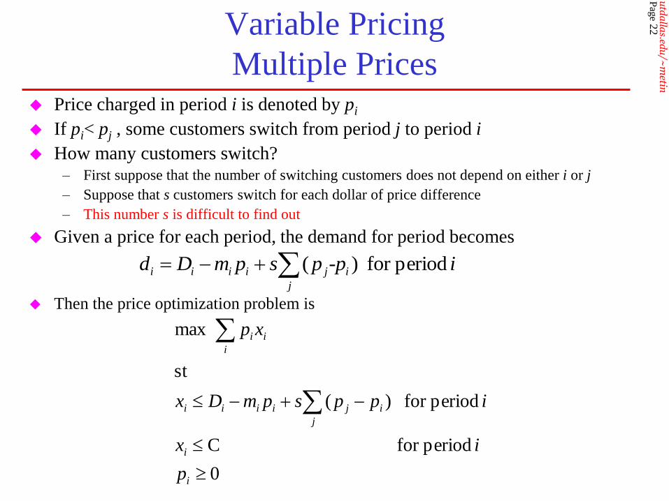
Variable Pricing

Multiple Prices Price charged in period i is denoted by pi

If pi< pj , some customers switch from period j to period i

How many customers switch?– First suppose that the number of switching customers does not depend on either i or j

– Suppose that s customers switch for each dollar of price difference

– This number s is difficult to find out

Given a price for each period, the demand for period becomes

0

periodfor C

periodfor )(

st

max

i

i

j

ijiiii

i

ii

p

ix

ippspmDx

xp

i-ppspmDd i

j

jiiii periodfor )(

Then the price optimization problem is

Pag

e23

utdallas.edu/~metin

Variable PricingRevenue of Multiple Prices > Revenue of Single Price

The multiple price formulation can be reduced to the single price formulation by inserting the following set of constraints

ippi periodfor

Inserting this constraint makes the objective value worse.

In other words, revenue can be made higher with multiple prices.

Pag

e24

utdallas.edu/~metin

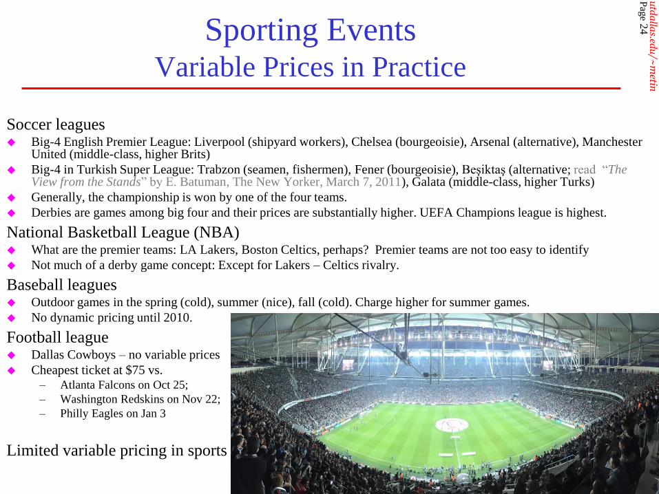
Sporting EventsVariable Prices in Practice

Soccer leagues Big-4 English Premier League: Liverpool (shipyard workers), Chelsea (bourgeoisie), Arsenal (alternative), Manchester

United (middle-class, higher Brits)

Big-4 in Turkish Super League: Trabzon (seamen, fishermen), Fener (bourgeoisie), Beşiktaş (alternative; read “The View from the Stands” by E. Batuman, The New Yorker, March 7, 2011), Galata (middle-class, higher Turks)

Generally, the championship is won by one of the four teams.

Derbies are games among big four and their prices are substantially higher. UEFA Champions league is highest.

National Basketball League (NBA) What are the premier teams: LA Lakers, Boston Celtics, perhaps? Premier teams are not too easy to identify

Not much of a derby game concept: Except for Lakers – Celtics rivalry.

Baseball leagues Outdoor games in the spring (cold), summer (nice), fall (cold). Charge higher for summer games.

No dynamic pricing until 2010.

Football league Dallas Cowboys – no variable prices

Cheapest ticket at $75 vs.– Atlanta Falcons on Oct 25;

– Washington Redskins on Nov 22;

– Philly Eagles on Jan 3

Limited variable pricing in sports

Pag

e25

utdallas.edu/~metin

Baseball League - Update in 2010Variable Prices at San Francisco Giants

San Francisco Giants experienced with dynamic pricing in 2009 season

They implemented it in 2010 season; revenue up by 6% with similar attendance figures

Ticket price depends on – Data from the secondary ticket market (ticket agencies)

– Status of the pennant race

– Success of Giants on the field

– Opposing team, higher prices withHistoric rivalry: Giants versus Dodgers

Pennant (e.g., National League West title) contenders

Rarely seen inter-league teams (such as Yankees)

– Pitching match-ups

– Day of the week

– Weather forecast

Example ticket prices for Giants vs. San Diego Padres game on Oct 1– Left-field upper deck stand: $5 at the start of the season; $5.75 on Aug 1, 2010; $20 after Giants

and Padres become contenders of NL West title

– Field Club behind home plate: $68 at the start of the season; $92 on Aug 1, 2010; $121 on Aug 9, 2010; $145 on Sep 4, 2010; $175 before the game.

– Prices went up as Giants were competing to advance to playoffs first time since 2003.– See Page 4 of ORMS Today , October 2010 Issue, Vol.37, No.5.

Pag

e26

utdallas.edu/~metin

Passenger AirlinesVariable Prices in Practice

Southwest (discount) airlines– Limited customer segmentation

– If demand for the next weekend’s morning flight to Chicago-Midway is high, increase price.

Other airlines (full-service) airlines– Customer segmentation

– Take coach class and split into fare classes

– Some classes are more expensive than others

– If demand is high, close low-fare classes

Pag

e27

utdallas.edu/~metin

Electric PowerVariable Prices in Practice

Peak electricity demand at 6 pm

Off-peak electricity demand at 4 am

Power generation from coal, nuclear, etc. – Big generators are on throughout the day, smaller ones are turned

on during peak periods

– Smaller generators are not efficient so their electricity is more costly

– A 5% reduction in electricity production during peak period reduces marginal cost by 55%

Reduce the demand during the peak period by increasing the price

Adjusting price with demand is not fully implemented– Historical reasons: Electric utilities were monopolies in local

markets

– Political reasons: Power companies generated little electricity to keep prices high in California. Then governor Davis was recalled and Schwarzenegger replaced him.

– US electricity grid is not integrated – east , west and Texas. ERCOT: Electric Reliability Council of Texas manages the flow of electric to 22 million Texas customers - representing 85 percent of the state's electric load and 75 percent of the land area.

Isolated applications in US: Recallable capacity (Industrial

Demand Response) in Ercot, NYISO and PJM markets.

Grid in 2010 above; Proposal with AC-DC-AC

connections below.

Pag

e28

utdallas.edu/~metin

Television AdvertisingVariable Prices in Practice

During a 30 min program, 3 pods of advertisements are shown. A pod lasts 150 sec.

Pods during prime time are more demanded than those during insomnia time

Advertisement buyers require a certain number of viewers for pods– Program ratings are important

Upfront market– For Fall, it lasts 1-2 weeks in May or June after the announcement of the Fall schedule

– Broadcaster guarantee of a number of viewers

– To fulfill the guarantee, broadcasters run additional advertisements (makeups)

– Broadcaster do not charge extra when there are more viewers than guaranteed

– How to fulfill the guarantee without overshooting it?» Issue: Number of viewers is not known in advance

Scatter market– Scatter market for Fall happens in Fall

– Scatter sales are cheaper and have no guarantees for the number of viewers

Constraints: No competing advertisements in the same pod; Not more than a certain number of advertisements for the same product in a single day.

Broadcasters have advertisement rate sheets (catalog prices) but give big discounts (pocket price is much less).

Pag

e29

utdallas.edu/~metin

Pricing with Constrained Supply

Summary

Pricing with a Supply Constraint

Opportunity Cost

– With and without market segmentation

Variable Pricing

Variable Prices in Practice– Sport events; Airlines; Electricity Markets; Advertising

Pag

e30

utdallas.edu/~metin

Market Segmentation with a Capacity ConstraintGraphical Depiction with Multiple Prices

Solution Method

40

8

16

ps

pg20 80/3

constraintcapacity ,8025.13 sg pp

Feasible

Price

Region

At the optimal prices, the capacity constraint is tangent to the ellipse.

If we treat student price as y-variable and the general price as x-variable, the slope of the capacity constraint is

25.1

3

d

d

g

s

p

p

This slope can be represented by either one of the following vectors:

[-1.25 3] or [1.25 -3]

[1.25 -3]

[-1.25 3]

Levelcurvesfor the

distorted circle

(0,0)

Pag

e31

utdallas.edu/~metin

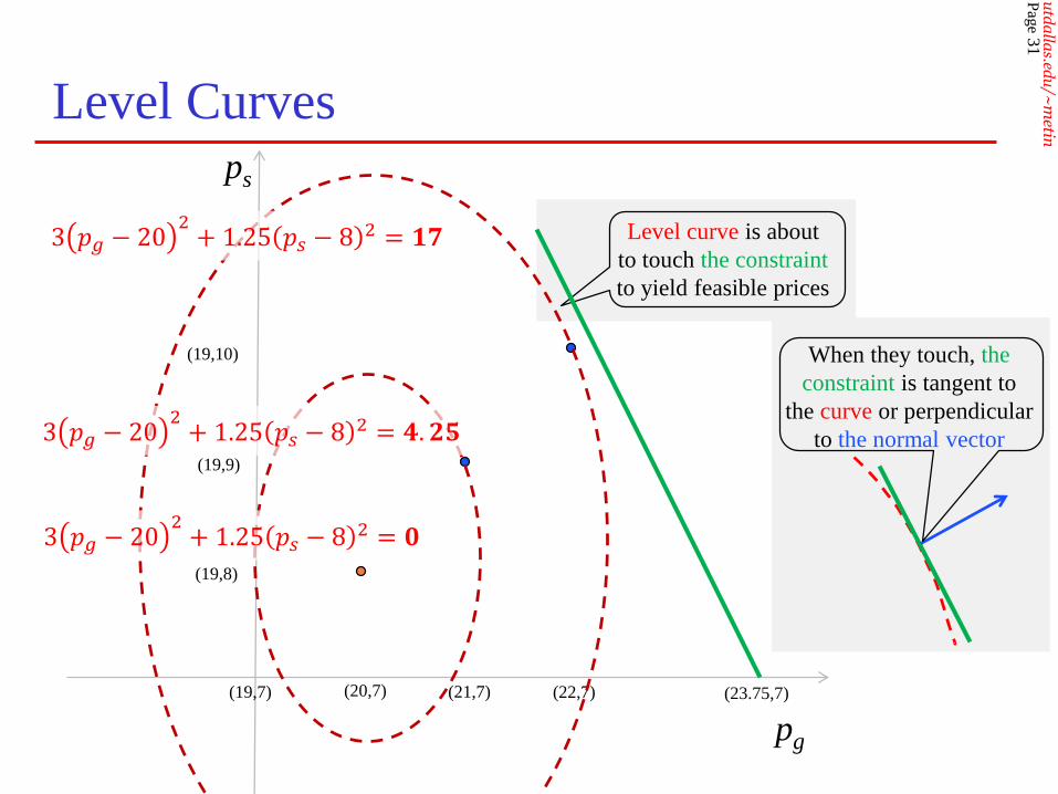
Level Curves

(19,8)

(19,9)

ps

pg

(20,7) (21,7) (22,7) (23.75,7)

(19,10)

(19,7)

3 𝑝𝑔 − 202+ 1.25 𝑝𝑠 − 8 2 = 𝟏𝟕

3 𝑝𝑔 − 202+ 1.25 𝑝𝑠 − 8 2 = 𝟒. 𝟐𝟓

3 𝑝𝑔 − 202+ 1.25 𝑝𝑠 − 8 2 = 𝟎

Level curve is about

to touch the constraint

to yield feasible prices

When they touch, the

constraint is tangent to

the curve or perpendicular

to the normal vector

Pag

e32

utdallas.edu/~metin

Normal Vectors to Level Curves

(19,8)

(19,9)

ps

pg

(20,7) (21,7)(19,7)

∙ Gradient vector of a curve is normal (perpendicular)

to the curve. Given a curve Π 𝑝1, … , 𝑝𝑛 =constant, the associated gradient is

𝛻Π =𝜕Π

𝜕𝑝1, … ,

𝜕Π

𝜕𝑝𝑛

∙ Given the curve for the ellipse

Π 𝑝𝑔, 𝑝𝑠 = 3 𝑝𝑔 − 202+ 1.25 𝑝𝑠 − 8 2 = 17

the associated gradient is

𝛻Π = [2 2 𝑝𝑔 − 20 , 1.25 2 𝑝𝑠 − 8 ]

∙ For example, at (𝑝𝑔 = 𝟐𝟐, 𝑝𝑠 = 𝟏𝟎) the gradient is

𝛻Π = 3 2 22 − 20 , 1.25 2 10 − 8

= 4 3, 1.25 ∝ [3,1.25].

At 𝟐𝟐. 𝟑𝟖, 𝟖 = (20 + 17/3, 8) the gradient is

𝛻Π = 3 2 22.38 − 20 , 1.25 2 8 − 8 ∝ [1,0].

At (𝟐𝟐, 𝟔) the gradient is 𝛻Π = 3 2 22 − 20 , 1.25 2 6 − 8

= 4 3,−1.25 ∝ [3,−1.25].

𝛻Π =[3, 1.25]

(19,6)

(19,10)

3 𝑝𝑔 − 202+ 1.25 𝑝𝑠 − 8 2 = 17

(22,10)

(22,6)

(22.38,8)𝛻Π =

[1, 0]

𝛻Π =[3, -1.25]

𝛻Π

Pag

e33

utdallas.edu/~metin

Market Segmentation with a Capacity ConstraintObtaining the Optimality Condition with Multiple Prices

Two vectors are parallel if they are a positive multiple of each other.

Two vectors are perpendicular if their scalar product is zero

03]- ;1.25][1.25 [3,

02]- 6][4; [3,

01] 6][-2; [3,

0-30] 6][-1; [3,

0183] 6][0; 3,[

Only the last three pairs of vectors are perpendicular above.

We want the gradient of the objective to be perpendicular to the vector representing the slope of the capacity constraint:

3 2 𝑝𝑔 − 20 , 1.25 2 𝑝𝑠 − 8 1.25;−3 = 3 2 1.25 𝑝𝑔 − 20 − 𝑝𝑠 − 8 = 0

So 𝑝𝑔 = 𝑝𝑠 + 12.

Pag

e34

utdallas.edu/~metin


Solution with Multiple Prices

40

8

16

ps

pg20 80/3

Feasible

Price

Region

We intersect two lines 3𝑝𝑔 + 1.25𝑝𝑠 = 80 and 𝑝𝑔 = 𝑝𝑠 + 12 to find optimal prices

𝑝𝑔 = 22.35 and 𝑝𝑠 = 10.35. Then Π 𝑝𝑔 = 22.35, 𝑝𝑠 = 10.35 = 4.25(2.35)2=23.47.

12

3 𝑝𝑔 − 202+ 1.25 𝑝𝑠 − 8 2 = 23.47

3𝑝𝑔 + 1.25𝑝𝑠 = 80

capacity constraint

𝑝𝑔 = 𝑝𝑠 + 12

𝛻Π

pricing with constrained supply - the university of …metin/or6377/folios/constrained.pdfe 1 u /~...

Documents