Department of Real Estate and Construction Management Thesis no. 320 Real Estate Development and Financial Services Master of Science, 30 credits Real Estate Management

Authors Supervisor Filip Gustavsson Simon Vahtola Stockholm 2014

Hans Lind

Pricing Strategies

in newly developed housing projects

II

Master of Science Thesis

Title Pricing Strategies – In newly developed housing projects

Authors Filip Gustavsson and Simon Vahtola Department Real Estate and Construction Management Master Thesis number 320 Supervisor Hans Lind Keywords Pricing Strategies, Real Estate, Housing

Development, Time-on-market, List price, Selling Price

Abstract

Earlier studies examining house pricing have mainly focused on the secondary market and

have often overlooked the primary market and newly produced housing units. This paper

studies the pricing strategies in the primary housing market, as that segment differs from the

secondary market.

By using data from one newly produced housing project, we are able to exclude a number of

project-specific factors, as they are nearly identical for all observations. This allows us to

focus on factors that are directly observable and require very little assessment or evaluation in

our estimations of list prices, selling prices and selling times.

The empirical results exhibit a close relationship between list- and selling prices, but a few

factors differ significantly between the two. Such differences could indicate a

misinterpretation of the market by the seller. The time-on-market model shows that a number

of factors affect selling times as well. The results indicate a relationship between “mispriced”

factors and their impact on the selling times, where “over-priced” factors seem to prolong the

time-on-market and “under-priced” factors seem to shorten the time-on-market.

By dividing the units into different price ranges, it becomes clear that high-priced housing is

more difficult to price and take longer to sell. This relationship is strengthened by a degree-of-

overpricing variable, which exhibits a positive sign in the time-on-market model. The effect is

the strongest in low-priced units and not significant for higher-priced units.

Other factors that affect pricing strategies require a broader discussion. Analogies from

similar consumer good markets indicate that pricing strategies are dependent on the types of

customers in the target groups as well as the stage in the project life-cycle.

III

Acknowledgment

“Price ain’t merely about numbers, it is a satisfying sacrifice” -Toba Beta

Thanks to those that we had the pleasure to meet along the way for your support and a special

thanks to Professor Hans Lind for his invaluable guidance.

Stockholm, May 25th

2014

Filip Gustavsson and Simon Vahtola

IV

Table of contents

1. Introduction ....................................................................................................................... 1

1.1 Background ....................................................................................................................... 1

1.2 Purpose ............................................................................................................................. 1

1.3 Limitations ........................................................................................................................ 2

1.4 Conceptual framework ..................................................................................................... 3

2. Methodology ......................................................................................................................... 4

2.1 Choice of method ............................................................................................................. 4

2.2 Data description and collection ........................................................................................ 4

2.3 Credibility of the study ..................................................................................................... 6

3. Theories of pricing strategies .............................................................................................. 7

3.1 Price discovery .................................................................................................................. 7

3.2 Search market vs. Auction ................................................................................................ 8

3.3 List Price and Anchoring ................................................................................................... 9

3.4 Time-on-market or selling speed .................................................................................... 10

3.5 Retail pricing strategies .................................................................................................. 12

4. Price and sales data ............................................................................................................ 15

5. What customer value factors explain the prices within the project? ............................ 17

5.1 Listing and selling price models ...................................................................................... 17

5.2 Differences between listing and selling price ................................................................. 20

5.3 Summary ......................................................................................................................... 21

6. What factors explain differences in selling times in the project? .................................. 22

6.1 Time-on-market model ................................................................................................... 24

6.2 Practical example of factor effects on time-on-market ................................................. 28

6.3 The effect on time-on-market in different price-ranges ................................................ 29

V

6.4 Summary ......................................................................................................................... 32

7. What could affect pricing strategies in housing development? ...................................... 33

7.1 Early sales performance ................................................................................................. 33

7.2 Demand variation – Leaders vs followers ...................................................................... 36

7.3 Marketing & spill over effects ........................................................................................ 37

7.4 Limited Supply ................................................................................................................ 38

7.5 Summary ......................................................................................................................... 39

8. Conclusions ......................................................................................................................... 40

Reference list ........................................................................................................................... 42

1

1. Introduction

1.1 Background

Throughout history, the supply of housing has been essential for a well-functioning society.

Over time, the market has taken on the task to deliver new supply and a prerequisite for the

developer to do this is that it can be done in a profitable and time-efficient manner.

In real estate development, as in other consumer markets, some of the largest challenges have

always been pricing of the units and the time it takes to sell them. This is especially apparent

in the housing market, where a large number of factors affect the final sales price and the

fluctuations in demand. The main focus of previous research has been the secondary housing

market, since most transactions take place there and because the largest values exist in that

market. Despite this, the primary housing market is subject to many transactions each year,

and large values change hands in the primary market each year as well.

When comparing the real estate sector to other sectors, it becomes clear that pricing strategies

are just as important when selling housing units as when selling other goods. This is despite

the fact that real estate comes with unique features that are very rare in other sectors, such as a

fixed locational attribute and a long product life-cycle.

When realizing the values that are dependent on pricing strategies, it becomes important to

examine how developers operate and how they set their prices. Developers that are involved

in larger projects with numerous phases over longer periods are more dependent on long-term

strategies, because their actions have longer repercussions and their early efforts affect the

performance of later phases. Pricing strategies in housing are also important to examine

because the pricing of units that have never been sold before differs somewhat from the

pricing of older units that have transacted numerous times. The most obvious difference is the

selling process of a newly developed unit, which is usually set up as “first come, first serve”

whereas the selling process of older units is often set up as a negotiation between sellers and

buyers.

By investigating a real estate development company that is developing areas with

multi-family apartment units, we are able to examine which variables have affected the sales

performance during the total life of the development.

1.2 Purpose

The purpose of this study is to identify variables that affect sales prices, time-on-the-market

and pricing strategies within a new housing development project.

Research questions

What customer value factors explain the sales prices within a project?

What variables influence time-on-market for new housing development?

What could affect pricing strategies in housing development?

2

The rationale for doing this study is to understand and improve current pricing practices in the

real estate industry as well as improving the knowledge base of pricing newly developed real

estate units.

The issues raised pose a problem to the entire real estate industry as the world becomes more

complex and integrated. As more factors and events affect the pricing of housing units, it

becomes increasingly difficult to identify what is affecting sales prices. The sales price and

sales speed are closely related, as the real estate market is a search market where a lower

seller reservation price generates a higher number of matches between the seller and potential

buyers. The problems that many developers face is what price level to choose in the first

stages of a housing development project. On one hand the developer can choose to set a low

price in order to raise interest and generate a positive word-of-mouth effect and risk losing a

price premium. The adverse effect of this could be that sharp increases in the price level in

later stages generate a negative effect on potential buyers that were enticed by the low initial

prices. On the other hand the developer can choose a high price level and earn a price

premium from the start. But if the price level turns out to be too high the company may have

to sell the later phases at a lower price, lowering the general price level in that market, putting

future projects at risk.

The contribution of this study is that it only examines newly developed areas or the primary

market for real estate where the seller is a development company. Many earlier studies have

examined secondary housing markets, where both the sellers and buyers are usually private

persons. The study also adds to the business intelligence of development companies through

improved understanding of the market functions and price dynamics of the housing market.

1.3 Limitations

This study is limited to cover only one housing project in one housing market and the

majority of the data will come from a large housing developer. Even though the issues raised

in this thesis apply to all parts of the real estate industry, only the owner- occupied housing

sector is examined. The study is limited to a specific time period, namely from 2010 to the

first quarter of 2014. Data from a longer period of time and from a number of development

companies would be optimal, but acquiring this information would be both costly and time-

consuming, which causes it to fall out of the scope of this study.

The factors examined in this study are limited by their observability. Some factors have been

observable, but have been excluded due to poor quality of the data. Some factors have been

excluded because of their naturally limited impact on housing prices and selling times of

housing.

Despite these limitations, the findings can contribute to the understanding of housing markets

in general. Other development companies in other countries and their respective markets can

benefit from this study in what pricing strategies to use for newly developed housing.

3

1.4 Conceptual framework

One of the most well-known theories of real estate and housing valuation is that of hedonic

pricing (Rosen, 1974). The theory states that the value of a building or housing unit is a

function of all its characteristics, such as size, location, number of rooms etc. as well as the

general market conditions in which the unit is located. A number of studies have been made

using hedonic pricing models in order to understand how different variables or characteristics

affect the value of real estate (i.e, Eichholtz et al, 2010 & Strand, Vågnes, 2001). The

difficulty that then is generated is to determine the value that each of the characteristics have

to a seller and to potential buyers. The problem is also to determine the aggregate value of

factors, which is the price that a seller is willing to accept and a buyer is willing to pay for a

housing unit.

Another important factor in the selling process of real estate is the selling speed, or the time-

on-the-market (TOM). The time that it takes to sell a unit can vary a lot depending on the

different apartment characteristics, the initial listing price and the market conditions. One can

argue that a longer TOM allows a seller to search for a buyer that is willing to pay more than

others, which would generate a positive correlation between TOM and transaction prices

(Wheaton, 1990). On the other hand, one can argue that a unit that has been on the market for

a long time might become stigmatized among buyers as being faulty and therefore less

desirable, ultimately reducing the transaction price (Taylor, 1999). Because of its

characteristics, the selling process in the housing market is often described in a search

theoretic framework. Search theory explains the trade-off between the sellers’ listing price

and the time it takes to sell the unit, as the seller wishes to sell the unit at the highest possible

price at the shortest possible time (Yavas, 1992).

Furthermore, the initial list prices have been shown to have a significant effect on final sales

prices and the time-on- market. An “overpricing” strategy of a unit has a negative effect on

the final sales price and the time it takes to market the unit (Knight, 2002). The listing price

also serves as a strong signalling tool for the seller to show his lowest acceptable price.

Furthermore, a significant share of home buyers use the list price as the single most

influential factor that helps them determine their first price offer (Yavas & Yang, 1995).

As mentioned earlier, the research in the field is mostly focusing on the “secondary” housing

market, which is the equivalent of a “used goods” market. What the field seems to be lacking

is a focus on the primary housing market, how newly developed areas are priced and how the

list prices affect units that have never been sold before. It also lacks research on how TOM

affects the final sales prices in different stages of the development (Li, 2004). Logically, many

analogies can be drawn between the primary and the secondary housing market but there are

some aspects that differ significantly between the two. The most obvious differences include:

age of the unit, the seller being a development company and the selling process. In the

secondary market an auction-like process takes place where both buyers and sellers are

private persons, whereas in the primary market a more retail-like process takes place.

4

2. Methodology

2.1 Choice of method

This study uses previous research as a base for its methodology. As the primary aim is to

understand what factors influence prices and selling times of housing, ordinary least squares

regression models, OLS, are the most straightforward way of finding them and their

magnitude. Previous research points out that there is a simultaneity problem inherent in

testing selling times and prices of housing which means that it is difficult to distinguish

between the effects of selling times and prices as they affect each other and there is no clear

chain of causality. Therefore, two models have been formulated in order to test selling times

and prices separately, to solve for this problem. A similar approach with a two stage model

has been used in other studies (see Yavas & Yang (1995) and Li (2004)).

The first model in the study focuses on the list and selling prices of a specific housing project

and compares separate units (apartments) within the project, in order to fully determine the

factors that affect the prices and their magnitude. The model will also be used to retrieve a

degree-of-overpricing variable, which is used in the time-on-market model.

The second model focuses on the time-on-the-market of each apartment and aims to

determine the individual impact of a set of factors on the selling times. Both regression

models only includes sold units, as that is a prerequisite for an observation of selling prices.

The final definition of each model is presented in the results and analysis section.

In the final part of the study, it turns more to grounded theory and inductive reasoning when

the analyses of factors that affect pricing strategies are carried out. Due to data limitation and

the fact that less research has been done in this field it is more suited for inductive reasoning

and allows for the formulation of original ideas rather than confirming already established

paradigms.

2.2 Data description and collection

The bulk of the data has been collected in March 2014 from in-house market reports that go

back to 2008. It is also collected from an internal sales database of a large development

company covering one housing project that spans from the beginning of 2010 up to the date of

collection.

The remaining data has been derived by the authors based on information about the subject

project and a visit to the project site. The number of observations varies between 517 and 817

depending on the model and data accessibility.

5

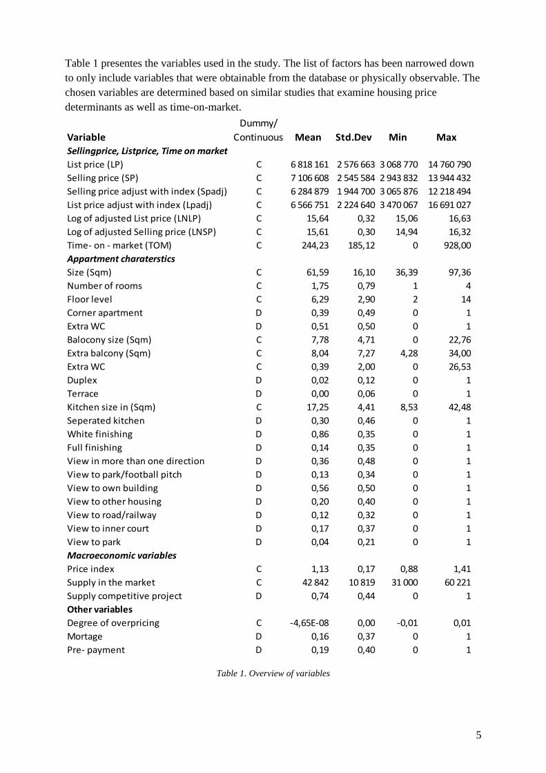
Table 1 presentes the variables used in the study. The list of factors has been narrowed down

to only include variables that were obtainable from the database or physically observable. The

chosen variables are determined based on similar studies that examine housing price

determinants as well as time-on-market.

Table 1. Overview of variables

Variable

Dummy/

Continuous Mean Std.Dev Min MaxSellingprice, Listprice, Time on market

List price (LP) C 6 818 161 2 576 663 3 068 770 14 760 790

Selling price (SP) C 7 106 608 2 545 584 2 943 832 13 944 432

Selling price adjust with index (Spadj) C 6 284 879 1 944 700 3 065 876 12 218 494

List price adjust with index (Lpadj) C 6 566 751 2 224 640 3 470 067 16 691 027

Log of adjusted List price (LNLP) C 15,64 0,32 15,06 16,63

Log of adjusted Selling price (LNSP) C 15,61 0,30 14,94 16,32

Time- on - market (TOM) C 244,23 185,12 0 928,00

Appartment charaterstics

Size (Sqm) C 61,59 16,10 36,39 97,36

Number of rooms C 1,75 0,79 1 4

Floor level C 6,29 2,90 2 14

Corner apartment D 0,39 0,49 0 1

Extra WC D 0,51 0,50 0 1

Balocony size (Sqm) C 7,78 4,71 0 22,76

Extra balcony (Sqm) C 8,04 7,27 4,28 34,00

Extra WC C 0,39 2,00 0 26,53

Duplex D 0,02 0,12 0 1

Terrace D 0,00 0,06 0 1

Kitchen size in (Sqm) C 17,25 4,41 8,53 42,48

Seperated kitchen D 0,30 0,46 0 1

White finishing D 0,86 0,35 0 1

Full finishing D 0,14 0,35 0 1

View in more than one direction D 0,36 0,48 0 1

View to park/football pitch D 0,13 0,34 0 1

View to own building D 0,56 0,50 0 1

View to other housing D 0,20 0,40 0 1

View to road/railway D 0,12 0,32 0 1

View to inner court D 0,17 0,37 0 1

View to park D 0,04 0,21 0 1

Macroeconomic variables

Price index C 1,13 0,17 0,88 1,41

Supply in the market C 42 842 10 819 31 000 60 221

Supply competitive project D 0,74 0,44 0 1

Other variables

Degree of overpricing C -4,65E-08 0,00 -0,01 0,01

Mortage D 0,16 0,37 0 1

Pre- payment D 0,19 0,40 0 1

6

Variable definitions

The first group of variables are different variations of prices for the units. Several of them are

adjusted with an index to make them comparable over time and some of them are logarithmic

as they are assumed to be non-linear1. Time-on-market is the difference between the selling

date and the listing date expressed as number of days.

The second group of variables include the physical characteristics of the apartments. Most of

them are straightforward, however some need an explanation. Extra balcony is defined as the

square metres of an additional balcony, if there is one. Separated kitchen means that there is a

separate kitchen and living room. Duplex is defined as a two-floor apartment. Basic finishing

is the standard design of finishing. Full finishing is an alternative with a higher overall

standard and additional equipment that the buyer can choose to order. Due to

multicollinearity, only full finishing is included in the models. The views are representations

of the major views from the apartments. There are six main views, of which one is to the inner

court. One apartment can have several views.

The macroeconomic variables include a property price index2 and two different supply

measures, of which one covers the whole market and one covers the launch of a nearby

housing project. The final group of variables include a measure of overpricing, as well as the

financing options chosen by the buyers of apartments. The measure of overpricing(DOP) is

derived from the first model in this study3.

2.3 Credibility of the study

In order to reach high credibility, a study needs to have good input data as well as a high level

of reliability and validity. The reliability of this study is not of any concern, as the methods

used will be conventional and easy to repeat in other contexts, other time periods and other

housing markets, as long as one has access to similar data.

The external validity can be questioned in these types of studies, as most research examines

one market and one sector of the real estate market during a specific period. In testing

hypothetical models, many researchers have narrowed their data set down to specific areas or

specific types of real estate. This is of course necessary, as the data still needs to be handled

and managed in an efficient way. It could lead to problems with generalizability, since only a

small part of the population is tested. This is a problem in this study as well, as the setup is

similar. The internal validity will be dependent on the model that is specified during the study

and it has to be designed to minimize measurement errors.

Finally, the study or the authors will not disclose neither the company from which the data is

obtained, nor the market which is examined. The data has also been manipulated as part of an

anonymity agreement.

1 See section 4.1 Price dynamics

2 Ibid

3 See the time-on-market model in section 4.3

7

3. Theories of pricing strategies

In this section an introduction to the theories in the field of pricing strategies is provided. The

areas discussed include price discovery and the difference between search markets and

auction markets. An introduction is also given of the importance of list prices and their

anchoring effects as well as the relationship between pricing and the selling speed or time-on-

market(TOM).

3.1 Price discovery

Several studies have been carried out to examine Price Discovery. The process is part of the

pricing of all goods and services, including the real estate market. The process is ongoing and

continues for the entire life-cycle of a product, as it is sold again and again. The information

can also be transmitted between different markets that share similar characteristics (Barkham

& Geltner, 1995), this applies, for example to the relationship between the real estate market

and the stock market, where shares in real estate companies and Real Estate Investment Trusts

(REITs) are traded.

Price discovery “is a process of information aggregation, through which market participants’

opinions about the value of an asset are combined into a single statistic, the market price of

the asset” (Barkham & Geltner, 1995).

Generally, Price discovery is seen as the level of transparency and information availability on

a specific market. A higher number of market participants and transactions allow information

about certain goods to flow faster and affect the price more quickly. Price-relevant

information can include both macro-economic and asset-specific variables, such as

unemployment rates or changes in taxation legislation. Markets with poor flow of information

have to rely more heavily on market aggregates, such as indices, or on information about

other markets that share some pricing determinants with the subject market. This may result in

a market or selling price that is different from the fundamental or “true” value (Geltner,

MacGregor, & Schwann, 2003).This means that the higher the number of transactions and the

more homogeneous the assets are and the simpler it is to observe the transaction prices, the

closer the distributions of buyer and seller reservation prices will be to a true value (Geltner,

Miller, Clayton, & Eichholtz, 2007).

The real estate market involves lengthy processes from project initiation to final sales and

project completion, the price discovery process is complex and incorporates a lot of

assumptions from the determination of an initial list price to the final sales prices adjusted for

discounts or other non-monetary benefits. Real estate differs in many ways from other goods,

with the most obvious being the geographical segmentation, long life-cycle, low liquidity,

unique objects and high capital requirements (Geltner, Miller, Clayton, & Eichholtz, 2007).

8

All features that set real estate aside from other goods affect the price discovery process, since

the lack of liquidity and comparable sales

imply a need for appraisals in the sales

process. These appraisals partly lean on

public information combined with

historical data which generate a certain

level of uncertainty. Despite this problem,

the real estate market still functions

relatively well, as there usually is a

sufficient number of trades and level of

homogeneity that accommodate more

accurate appraisals (Geltner, MacGregor,

& Schwann, 2003).

3.2 Search market vs. Auction

The selling of real estate is a time-

consuming process. It is closely

intertwined with the price discovery

process. It is in the selling process that one

can observe some reservation prices of

both buyers and sellers and identify the

intervals in which a transaction can be reached.

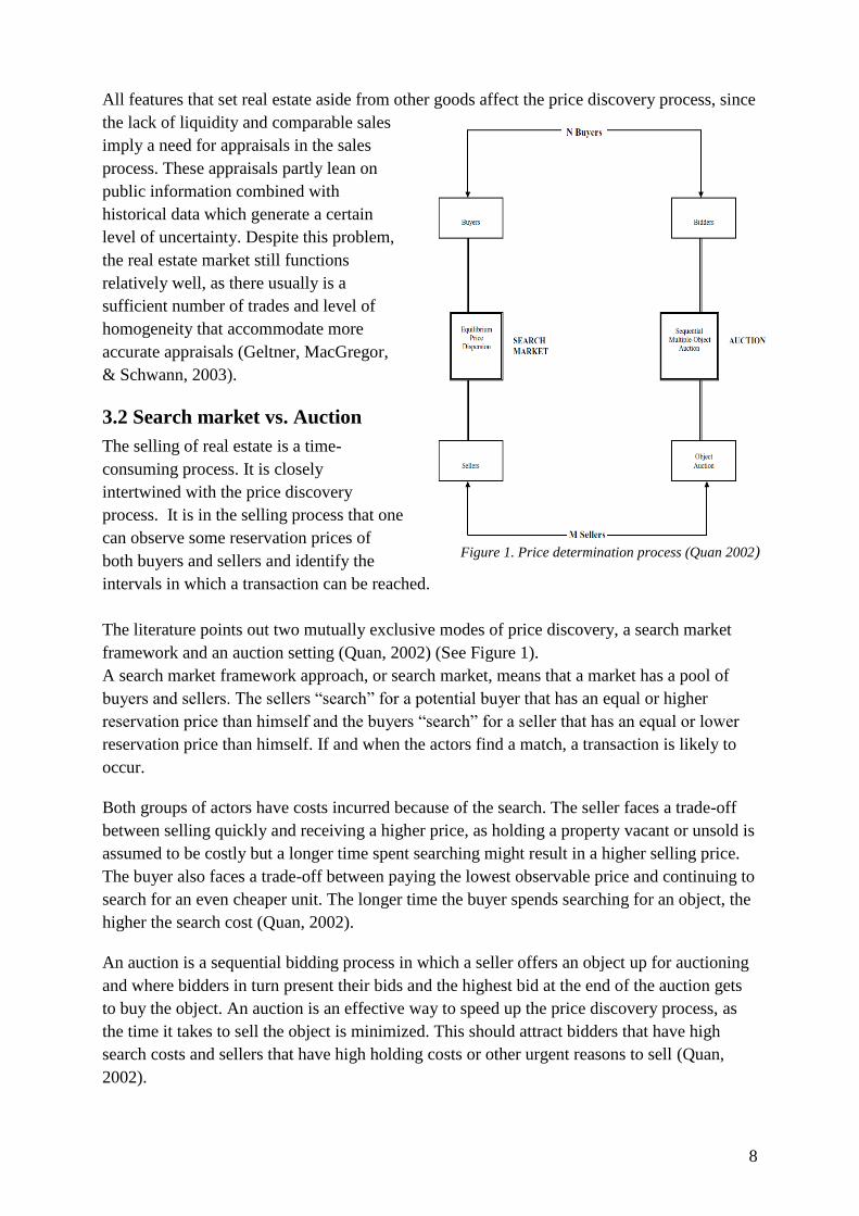
The literature points out two mutually exclusive modes of price discovery, a search market

framework and an auction setting (Quan, 2002) (See Figure 1).

A search market framework approach, or search market, means that a market has a pool of

buyers and sellers. The sellers “search” for a potential buyer that has an equal or higher

reservation price than himself and the buyers “search” for a seller that has an equal or lower

reservation price than himself. If and when the actors find a match, a transaction is likely to

occur.

Both groups of actors have costs incurred because of the search. The seller faces a trade-off

between selling quickly and receiving a higher price, as holding a property vacant or unsold is

assumed to be costly but a longer time spent searching might result in a higher selling price.

The buyer also faces a trade-off between paying the lowest observable price and continuing to

search for an even cheaper unit. The longer time the buyer spends searching for an object, the

higher the search cost (Quan, 2002).

An auction is a sequential bidding process in which a seller offers an object up for auctioning

and where bidders in turn present their bids and the highest bid at the end of the auction gets

to buy the object. An auction is an effective way to speed up the price discovery process, as

the time it takes to sell the object is minimized. This should attract bidders that have high

search costs and sellers that have high holding costs or other urgent reasons to sell (Quan,

2002).

Figure 1. Price determination process (Quan 2002)

9

The drawback with participating in an auction is that it ignores face-to-face bargaining

between the buyer and the seller which in turn takes place in the search market setting. What

remains is the “bargaining” between the buyers, which can result in a “bidding war”. There

are numerous examples of auctions that have failed, or where the objects have remained

unsold. Although unsuccessful, this may still serve as a valuable exposure of the objects, since

the process identifies potential buyers and their reservation prices, which allows the seller to

modify his expectations and strategy regarding the unit (Ong, 2006).

3.3 List Price and Anchoring

As mentioned earlier, the selling of real estate and housing is a lengthy process, and one of the

most important and crucial parts of the process is for the seller to choose an initial price at

which the house is listed on the market. This listing price affects the ultimate selling price and

the time it takes to find an able and willing buyer, or marketing time. Worth noting is that the

decision about the list price does not have to be final. A seller can adjust his list price

according to the initial reactions from the market, as he learns about the market demand for

his unit (Knight, 2002). Read (1988) also shows how a sequence of list prices can be used by

a profit-maximizing seller to reach an optimal reservation price.

The list price can also be viewed as an initial offer made by the seller to potential buyers in

the bargaining game set up by the seller to which buyers can respond in three ways: accept,

reject and continue searching in the market or bargain with the seller (Arnold, 1999).

There is a strong relationship between the list price and the sales speed. A high list price

relative to value reduces the number of potential buyers and consequently increases the time it

takes to sell the unit (resulting in a higher holding cost). A low list price increases the

possibility for a fast sale, as the number of buyers increases, but at the same time risking a

sales price which ends up lower than what could have been achieved with a longer marketing

time (Knight, 2002). The risk that a seller is facing, in the case of a house being on the market

for a long time is a stigmatization effect, which can have a severe negative effect on the final

sales price. This effect arises when weary buyers suspect that a house has an unobservable

fault, which is causing it to remain unsold (Taylor, 1999).

Setting the correct list price is of crucial importance as a revision of the list price has been

shown to have a negative effect on the final sales price of the property (Knight, 2002).

Another problem is that “overpriced” properties also end up with a lower selling price. This

shows that a seller has to be careful in setting a too high list price as it reduces the number of

possible buyers and increases the risk of stigmatizing the property.

There are a number of aspects regarding the list price that affects the outcome of the selling

process, with one of the most central being the signalling effect that is inherent with the list

price. The list price sends a signal to the buyer about the reservation price of the seller and

provides the pool of buyers with an upper bound (the price at which a seller is willing to sell

10

immediately) (Yavas & Yang, 1995). The negotiation then takes place in an interval between

the sellers reservation price (the lower bound) and the list price (the upper bound)4.

A lot of research has been done on a feature of list prices called the anchoring effect. This can

be described as a psychological bias that distorts the perceptions of buyers about the value of

a potential unit. This can result in a “mispricing” of real estate if buyers cannot correct for the

sellers ambition to “anchor” the price above a fair market value (Bokhari & Geltner, 2011).

Some studies have shown, quite contradictory to the theories on stigmatization and

overpricing mentioned above, that a higher list price generally leads to higher valuations by

buyers compared to setting a lower list price. This has been shown by letting different groups

value the same property and with the same information except the list price, where one group

has received a high list price and one group has received a low list price. In these cases it was

easy to establish that the anchoring effect has a clear impact on valuations made by buyers

(Northcraft & Neale, 1987) (Bucchianeri & Minson, 2013)). This further strengthens the

importance for the seller to consider his listing price and interpret the market.

It has been shown that most professionals often recommend an under-pricing strategy, when

in fact a higher list price generates a higher sale price. An explanation to why under-pricing

sometimes works is that it is related to the market thickness or the number of interested

buyers in the market. The idea of seeking “bidding wars” is exaggerated as they only occur in

“hot” markets. An idea to why under-pricing is used so frequently is the realtors wish to sell

the house as quickly as possible, another being the fact that successful stories of “bidding

wars” get more attention than regular house sales experiences, which in turn leads to a greater

belief in under-pricing strategies (Bucchianeri & Minson, 2013).

3.4 Time-on-market or selling speed

Together with the selling price, the time-on-the-market (TOM) or marketing time is one of the

most important factors that the seller has to consider when divesting a property. One question

that the seller has to ask himself is whether or not he will receive a higher selling price if he

waits longer for a buyer or if he will be better off by selling the property at the current price.

The TOM and its interaction with the selling price has been studied with several perspectives,

namely its correlation with selling prices, the price concession ratio(the ratio of selling price

and list price) and search theory (Kalra & Chan, 1994).

The relationship between TOM and selling price has proven to be difficult to fully determine,

as previous research points in different directions. Some studies say the correlation is positive

(i.e Asabere, Huffman, & Mehdian, 1993) while others claim it to be negative

(i.e Cubbin, 1974).

The relationship between TOM and the price concession ratio has been proven to consist of a

negative correlation as a higher degree of “overpricing” generates a longer TOM. This means

that houses that have sold for a lower price than the listing price, have generally taken a

4 The idea that the listing price provides an upper bound is in the author’s opinion a market specific feature, as

it is not uncommon in other markets for the ultimate selling price to be higher than the listing price.

11

longer time to sell compared to houses that have sold at or above their listing price. The

correlation has proven to be significant for all house price ranges and especially for high-price

units that seem highly affected by differences between list prices and selling prices (Kalra &

Chan, 1994). TOM has also been shown to have a positive correlation with the standard

deviation of prices. A wider distribution of prices is suggested to make it easier for the seller

to wait for a higher price in the future, which leads to a longer TOM (Hui & Yu, 2012).

The relationship between TOM and Search theory has been the subject of a number of papers,

and as with selling price, the results point in opposite directions. Some state that a longer

selling time increases the probability of better offers, whereas others say that properties that

have been marketed for an overly long time might become stigmatized and sell for less (see

section on stigmatization) (Hui & Yu, 2012). An explanation to why different pricing

strategies occur could be shifts in the general economic trend as well as changes in the actors’

expectations about the future. If the market participants expect the market to turn downward,

it seems logical for the sellers to adjust their prices to accommodate this trend. In a downward

moving market, the best strategy for the seller is to sell the unit as fast as possible, or with a

short TOM. In a rising market, the market participants expect that prices will continue rising.

This implies that the buyers ought to make faster decisions, as prices will be higher in the next

period. In a rising market, the optimal strategy for the seller is to raise his asking price during

the marketing time, as it has little impact on his TOM (Hui & Yu, 2012).

Except the three dimensions described above, the relationship between TOM and seller

pricing strategies has also been a subject of research. A number of studies have shown that the

more overpriced an apartment is, the higher the TOM will be (Li, 2004), (Miller, 1978). It has

also been shown that under-pricing produces a sub-optimal selling price as the units are sold

too fast (Asabere, Huffman, & Mehdian, 1993). An explanation to why different pricing

strategies occur could be shifts in the general economic trend as well as changes in the actors’

expectations about the future.

In addition, some characteristics that affect the pricing of a housing unit, also affect its selling

time. For example, it has been shown that units at lower floors have higher TOMs while units

on higher floors, with good views and proximity to city centres have a lower TOM. Other

characteristics, such as the number of bedrooms or an extra toilet, did not act as determinants

of TOM (Li, 2004), (Ong & Koh, 2000). The atypicality of housing units has also shown to

have a negative effect on the TOM, meaning that properties with odd features take longer to

sell (Haurin, 1988).

Lastly, TOM has a strong correlation with the macroeconomic conditions in a market, such as

inflation, unemployment, a general property price trend and mortgage interest rates, as these

have a strong impact on both buyer and seller behaviour and the local market.

The impact of unemployment rates on the marketing times required can be large. In markets

with rising unemployment rates it seems logical to see longer TOMs, as buyers become

apprehensive toward taking on large risks and as sellers are unwilling to lower their asking

prices. The opposite can be expected in markets with declining unemployment rates, but one

could also expect sellers to adjust their asking prices to the trend, as they expect higher prices

12

in the next period, leaving the TOM unchanged. A very similar relationship can be seen

between the TOM and general property price trends (Hui & Yu, 2012).

The inflation factor is per definition negatively correlated with TOM. Ceteris Paribus, a higher

inflation today leads to lower real prices, which in turn raises the incentives to buy housing

today, as prices will be higher tomorrow (Leung, Leong, & Chan, 2002). Closely related to

the inflation rate are the mortgage interest rates. These have a similar relationship to TOM, as

a lower mortgage rate reduces the cost of living and boost the demand for housing, which in

turn should lead to shorter marketing time. This is especially apparent in the low-price

housing sector, as they are more sensitive to total costs of living (Kalra & Chan, 1994).

As pointed out, there is a strong relation between the housing and financial market conditions

and TOM. However, the impact of the separate variables is not always easy to distinguish.

The proven correlations often seem to be heavily dependent on the specific datasets and time

periods when the studies were carried out. This results in an somewhat ambiguous literature

and the importance of separate macroeconomic variables seems to differ across the field.

3.5 Retail pricing strategies

When introducing a new product to the market the seller needs to set an initial price, a process

which in some ways is associated with guesswork. This is especially apparent in the retail

market, such as clothing and cars where the price is set before any transactions have taken

place and then adjusted after a certain marketing period to better fit the demand. In the

secondary housing market the prices are usually reached through a haggling process between

the buyer and seller. Taking this into account, it means that the pricing in the primary housing

market has more in common with other retail goods than the pricing in the secondary housing

market has. This makes it interesting to investigate strategies of classic retail goods.

The simplest example of discovering price levels of consumer goods is to set an initial price,

observe the sales volumes and then adjust price in the next period until a satisfactory sales

volume is reached. For example, if the product does not sell well in the first period, it was

probably overpriced and the price should be lowered. In reality other factors need to be taken

into account, namely the number of customers and their homogeneity. Having a large number

of customers examine the product and rejecting is a more reliable signal of overpricing than a

small number of customers rejecting the product. The homogeneity or similarity among the

customers also affects the information value of selling more or less. If the product has been

targeted to the wrong market segment, the product may seem to be priced wrong, even though

there are other customers who are willing to pay the price (Lazear, 1986). So the

characteristics of customer groups is important for the real estate marketer of newly built

housing units who is attempting to put the first phase of a project for sale.

The density of markets (the number of potential customers) is an important factor for the

information value of sales performance. A larger number of potential customers and their

decisions allows a seller to adjust his or her pricing with more confidence and faster compared

to thinner markets. This means that products in denser markets have more volatile prices, and

clearance sales occur more frequently (Lazear, 1986).

13

The density of the markets is an assumption in itself, but some logical reasoning and

inferences from similar markets should provide some guidelines to the approximate amount.

For example, a $ 20,000 Fiat car reasonably has more buyers than a $ 3 million Lamborghini,

which in turn makes it easier to adjust the prices of the Fiat compared to the Lamborghini if

both have remained unsold for say 2 months. The fewer transactions a product has per unit of

time, the thinner the market is, like in the case of the Lamborghini.

In analysing the selling performance of a new product or project it is imperative to understand

the life-cycle of it, or the rate of adoption in the market. Theories on this matter have been the

subject of research for many decades, and one of the most cited is the one covering diffusion

curves of innovation (Rogers, 1962). It states that all new products are adopted (bought) by

their respective markets following a certain distribution. This is usually presented as a bell-

shaped curve (figure 2), where the leftmost area occupies the innovators and early adopters,

the centre area occupies the early and late majority and the rightmost area occupies the

laggards. The theory also states that there are five characteristics of a new product

(innovation) which influence the speed or rate at which it is adopted. These are:

Relative advantage, how much better is the product compared to the competitors?

Compatibility, how does the product match the values and experiences of the

customers?

Complexity, how easy is it to understand the product?

Divisibility, can the product be tested to any degree?

Communicability, how clear are the benefits of the product?

Figure 2. Diffusion curve of innovations (Rogers, 2003)

Newly built housing units could be said to be a mix of a number of innovations that

individually have to be adopted by the market as well as existing products that are already

adopted. The different innovations can also be in different stages in their life-cycle; the

location (as an innovation) might have reached adoption by the late majority, whereas the

architectural design of the buildings in a project might still only be adopted by the early

majority. Therefore the marketer has to have the consumer adoption process in mind when

targeting advertising to his market segment (Kotler & Keller, 2012).

14

Competitor strategy and consumer behaviour

Even though a developer of housing units in a specific location often has a monopoly in that

micro-market, he is still subject to competition from developers in other markets that offer

reasonable substitutes. Therefore housing development shares many aspects with an

oligopolistic market where pricing is used as a competitive tool. This also means that the

actions of the competitors have to be considered carefully when making decisions on the own

development project as it affects both prices and selling times on the market (Knight, 2002).

It is also important to remember that a housing developer is competing with existing supply in

the secondary market, as buying an old unit surely provides an option for most buyers as it is

less common to only search for newly built housing units.

In the same way that competitive sellers affect each other, competitive buyers also affect each

other’s choices. Having many or few rival buyers affects the time a buyer “dares” to wait for

the price to possibly fall. If there are many rival buyers a hesitant buyer runs a larger risk of

being left out of the market, therefore it is more likely that he “buys it when he finds it”.

(Lazear, 1986) This implies that the developer needs to consider the consumer behaviour

more when there are fewer buyers of specific apartments, such as expensive or high-end units.

15

4. Price and sales data

In the following chapters, the results and analysis of the study are presented. Factors that can

explain list and selling prices are discussed first, followed by a discussion of the factors that

cause differences between the two prices. Thereafter the variables affecting the time-on-the-

market are examined. Lastly, a broader discussion of other factors that affect pricing strategies

is presented. To give a better understanding of the background of the project and what has

affected the market during the studied period some price dynamics are provided and

compared with an index of the market price development.

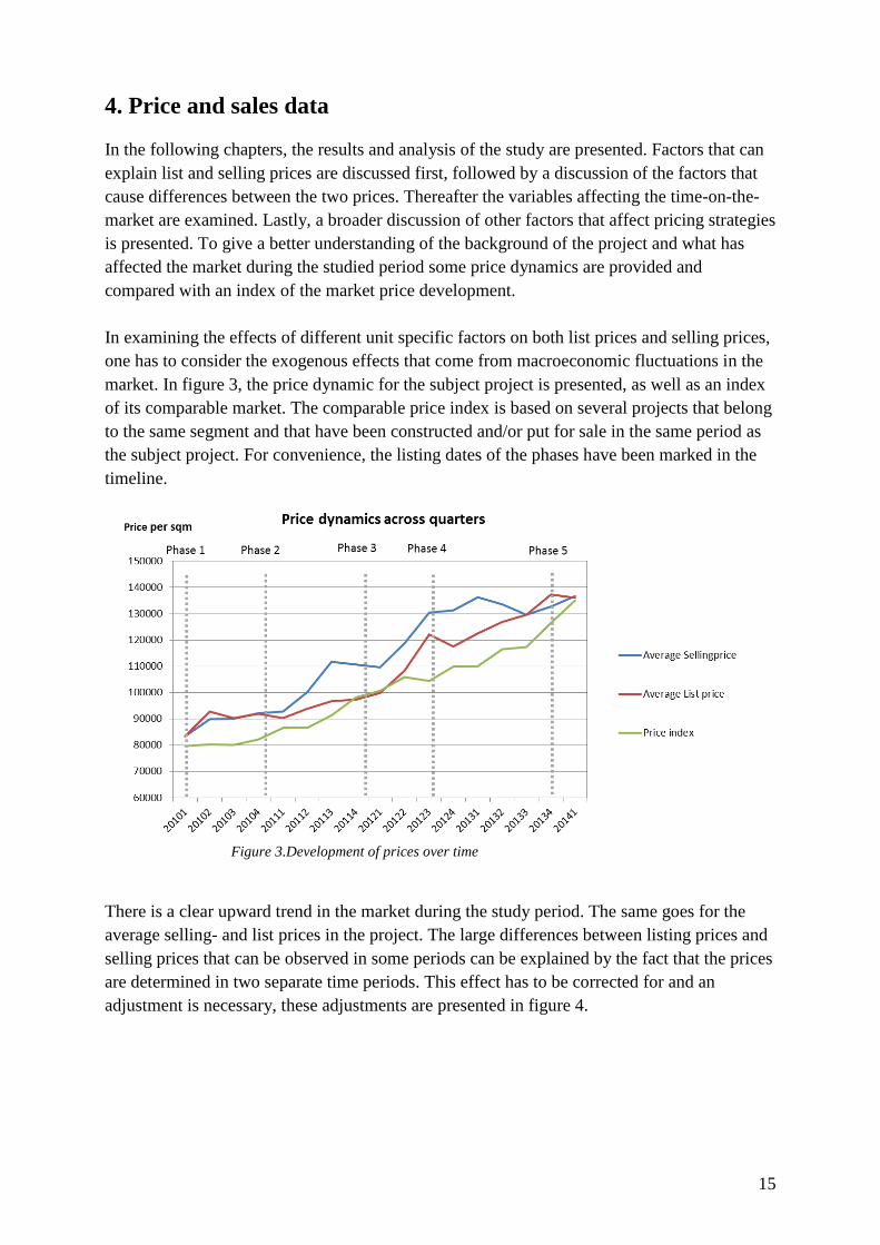
In examining the effects of different unit specific factors on both list prices and selling prices,

one has to consider the exogenous effects that come from macroeconomic fluctuations in the

market. In figure 3, the price dynamic for the subject project is presented, as well as an index

of its comparable market. The comparable price index is based on several projects that belong

to the same segment and that have been constructed and/or put for sale in the same period as

the subject project. For convenience, the listing dates of the phases have been marked in the

timeline.

Figure 3.Development of prices over time

There is a clear upward trend in the market during the study period. The same goes for the

average selling- and list prices in the project. The large differences between listing prices and

selling prices that can be observed in some periods can be explained by the fact that the prices

are determined in two separate time periods. This effect has to be corrected for and an

adjustment is necessary, these adjustments are presented in figure 4.

16

Figure 4. List-and selling price adjusted with price indices with different index values

The graph shows a price dynamic where both prices are adjusted with different index values.

The list prices are divided with the index values for the time when the unit was first listed and

the selling prices are divided with the index values for the time when the units were sold. A

frequency table of sold apartments in each period is also included to show the variance in

sales performance. This can explain the peak that is observable in March 2012 as the period

only had sales of three units that were all priced higher than average.

The graph also shows that the list price and selling price move more closely together

compared to the unadjusted prices. The prices also exhibit a more flat development over time

suggesting that the price index captures the macro-economic fluctuations well.

The adjustments enable us to compare all the sold units in the projects as we are able to

control for the time variable. This also allows us to use the adjusted prices when examining

the effects of unit specific attributes on list- and selling prices in the following section.

17

5. What customer value factors explain the prices within the

project?

This section investigates the prices at which units have been listed and sold within the subject

project. Since the list and selling prices sometimes differ from each other, the study examines

both prices separately in order to find differences and similarities between the two. The first

models aim at explaining the list-and selling price and is presented below.

5.1 Listing and selling price models

The equations (a) and (b) are log-liner models. The dependent variables ln LP and ln SP are

adjusted to the price index mentioned earlier in order to make the different units comparable

to each other over time. represents a set of physical attributes of apartments which have

been selected based on previous studies in the field. In the regression model, no locational

factors are considered as the units within the project are located in the same area. The macro-

economic effects are indirectly controlled for through the prices, which are adjusted with the

price index. is an error term which is supposed to capture the random variance in the

model and is a constant term.

The model has a strong explanatory power, as shown by an R-squared of over 90 percent for

both List price and Selling price. Most of the independent variables are significant on the one

percent level. This together with a high R-squared shows that the chosen variables effectively

explain variances in the log-transformed list- and selling prices. Not surprisingly, all variables

have the same sign when explaining both prices.

Table 2 shows variables that significantly explain list- and/or selling prices. The variables and

their individual impact are discussed below. The coefficients shown in the table are

percentage changes in the dependent variable that follows from a one-unit increase or

decrease in the independent variables.

(b)

(a)

18

Table 2. List and Selling price model

Apartment characteristics

Quite logically, the Size variable explains a lot of the variance of both list prices and selling

prices, as an apartment which is larger, ceteris paribus, should have a greater value to a buyer.

Number of rooms also has a big impact on the list and selling prices, as more expensive

apartments tend to have more rooms and bigger apartments usually have more rooms. An

increase in the size of one square metre raises both the list price and selling price by around

one percent and one more room increases both prices by around seven percent but the

relationship between the price and number of rooms is probably not perfectly linear and the

impact decreases for larger apartments.

Floor level also has a positive impact on prices, which is expected, since a higher floor level

provides a better view as well as quieter surroundings. One level higher increases both prices

by around two percent. An Extra WC is also closely related to size and should provide a

higher value to a buyer, which the model shows. However, the effect is slightly different

between list- and selling price as it increases list prices by around eight percent and selling

prices by around ten percent.

Separated kitchen has a negative coefficient, which is quite intuitive, since it implies that the

kitchen is separated from the living room and as a connected kitchen and living room is a

sought-after feature in the studied housing market. Having a Separated kitchen lowers the list

prices by about seven percent and selling prices by around five percent. Balcony size also has

a positive impact on prices, as a larger balcony should provide a higher value to buyers. One

Coefficient Prob Coefficient Prob

Size (sqm) 0,01 0,000 *** 0,01 0,000 ***

Number of rooms 0,07 0,000 *** 0,07 0,001 ***

Floor level 0,02 0,000 *** 0,02 0,000 ***

Full finishing 0,00 0,751 0,11 0,000 ***

Extra WC 0,08 0,000 *** 0,10 0,000 ***

Balcony size (Sqm) 0,01 0,000 *** 0,02 0,000 ***

Duplex 0,12 0,000 *** 0,09 0,006 ***

Terrace 0,37 0,000 *** 0,23 0,000 ***

Separated kitchen -0,07 0,000 *** -0,05 0,002 ***

View to more than one direction 0,08 0,000 *** 0,00 0,958

View to other housing -0,11 0,000 *** -0,05 0,000 ***

View to inner court -0,05 0,000 *** -0,02 0,128

View to park -0,02 0,224 -0,03 0,065 *

Supply competitive project -0,01 0,111 -0,03 0,000 ***

14,56 0,000 *** 14,56 0,000 ***

* Indicates a significance at the 10% level

** Indicates a significance at the 5% level

*** Indicates a significance at the 1% level

0,9497

0,9484

517

Selling Price

517

0,9257

0,9276

Dependent Variable

Independent Variable

Listing Price

Constant

R- Squared

Adjusted R-Squared

N

19

more square metre of balcony raises the list price by one percent and the selling price by two

percent, the marginal effect is reasonably declining. The same goes for apartments with

Terraces or Duplex. Both provide a value increase but this is also where the largest

differences in the coefficients can be observed, as both Duplex and Terrace increases list

prices more than selling prices.

Having ordered Full finishing presents an expected positive impact on selling prices and

raises the price by eleven percent. Obviously it can have no impact on list prices as they are

based on ordering no finishing (white finishing).

Views

The views take different signs and this is expected. View in more than one direction is

significant for list prices but not for selling prices. This implies that the developer has

considered this feature but not the buyers. Having a View to competitive project has a negative

impact on both prices, which is expected, but here a difference between the effects on selling

price and list price can be observed, as the effect is a lot larger on list price than on selling

price. View to inner court has an insignificant impact on selling prices but is significantly

negative for list prices. This is somewhat unexpected but could be explained by a large

variance in the dataset and difficulties in defining the variable. It has not been a consideration

for the buyers.

The most surprising result is the View to park, which is expected to be positive but instead

takes a negative sign, however insignificant for list prices. This could be explained by a

limited number of observations with a view to the park, since most apartments with this

feature can been seen in the last phase of the project and are not yet sold.

Another explanation to why some views exert slightly unexpected effects could be dependent

on how the model controls for macroeconomic fluctuations (adjustments to the prices with

indices) as some views have strong correlation to certain phases (i.e. different time periods) in

the project.

Views are also difficult to price due to the fact that each apartment has a unique view that is

difficult to generalize.

Supply competitive project

The variable Supply competitive project is a dummy variable indicating whether or not a

nearby competitive project has been put for sale when a specific apartment was sold. As

expected, the effect of the competitive project is negative, as an increased supply generally

lowers the equilibrium price level in a market. The model indicates that the effect of the rising

supply has not been considered when list prices have been set but in turn negatively affected

selling prices. One possible explanation to this is that the developer has not seen the other

project as fully competitive and therefore not adjusted prices in relation to the changed

supply.

20

5.2 Differences between listing and selling price

Large differences between the listing price and selling price could be an indication of

mispricing or misinterpretation of the market by the seller. Natural causes to large differences

between the prices are fluctuations in the average market prices as the listing prices are

determined some time before the listing of units and the selling prices could be determined

years after the listing date, a time during which markets may have fluctuated greatly,

significantly affecting prices. Aside from this, there are other reasons to why there could be a

large difference between the listing price and selling price. These are how well the supply that

is offered matches the buyer preferences and the relative pricing of specific attributes in a

housing unit.

To show the effect on differences between list- and selling prices, consider an example

apartment with given attributes and some changes.

Table 3. Example of effects on list- and selling price

The idea of this example is to clarify the similarities and differences in the effects of attribute

changes between list prices and selling prices. The table shows that Size, Number of rooms

and Floor level have the same coefficient in both list- and selling prices which results in the

same impact on both prices, given a certain change.

Both Extra WC and Balcony size have a larger impact on the selling price compared to the list

price, which can indicate that the buyers value these attributes higher than the developer

expected.

Example

Factors Attributes Change Coefficient

Change

in price Coefficient

Change

in Price

Size (sqm) 50 10 0,01 500 000 0,01 500 000

Number of rooms 1 1 0,07 350 000 0,07 350 000

Floor level 5 1 0,02 100 000 0,02 100 000

Full 0 0 0,00 0 0,11 0

Extra WC 0 1 0,08 400 000 0,10 500 000

Balcony size (sqm) 5 1 0,01 50 000 0,02 100 000

Duplex 0 0 0,12 0 0,09 0

Terrace 0 0 0,37 0 0,23 0

Seperated kitchen 0 0 -0,07 0 -0,05 0

View to more than one direction 0 1 0,08 400 000 0,00 4 000

View to other housing 1 1 -0,11 -550 000 -0,05 -250 000

View to inner court 0 1 -0,05 -250 000 -0,02 -100 000

View to park 0 0 -0,02 0 -0,03 0

Supply competitive project 0 1 -0,01 -50 000 -0,03 -150 000

Initial price 5 000 000 New prices 5 950 000 6 054 000

Selling PriceApartment List Price

21

View to more than one direction raises the list prices a lot more than the selling prices,

indicating an overestimation of the value of that attribute by the developer. The effect is not

even significant for selling prices. The opposite effect can be found for View to competitive

project and View to inner court, where the developer has underestimated the value of these

attributes.

The effects of Terrace and Duplex are not presented in the example. Both attributes raise the

prices significantly, but both exhibit stronger impacts on the list prices compared to selling

prices, again indicating an overvaluation. The Supply competitive project variable has a

stronger negative effect on the selling prices compared to list prices, which indicates

overpricing of this factor from the developer.

5.3 Summary

Through a price index adjustment, all sales have been made comparable. A number of factors

affect list- and selling prices. Most factors affect list and selling prices equally, including most

apartment specific features, such as size and number of rooms. However, some factors present

different effects on list- and selling prices. All factors have the same sign in both models, but

their magnitude differs greatly in some cases, such as the Supply and Duplex variables. A

difference between the initial listing price and the actual selling price could serve as an

indicator of a misinterpretation of the market by the seller, and factors that have different

magnitudes in the models could be a sign of mispricing of some factors.

22

6. What factors explain differences in selling times in the project?

The profitability of a property development project is not solely dependent on the price that

one can receive for a specific unit. It is also dependent on the time it takes to sell the different

units, as real estate projects incur large capital costs that accumulate over time until the units

are sold or in other words, it is costly to hold unsold apartments as they do not generate cash

flow. Therefore it is interesting to examine if there are attributes or factors that can explain the

selling times of apartments in a project. It is reasonable to argue that the different qualities of

an apartment are captured by its price and it is reasonable that all apartments should have

similar selling times or sell at the same pace on the market. Therefore no physical attributes

should be able to explain significant differences in selling times. The results of this study

show that this is not the case and there are a number of factors that significantly explain

differences in selling times.

Figure 5 and 6 depict the frequencies of sold apartments over their time-on-market, which is

defined as the period between the listing date and the selling date. This means that the first

phase naturally has some units with a longer TOM compared to the fourth phase which has

only been on the market for around 500 days.

Figure 5. Aggregated frequency of apartments sold over their time-on-market.

The frequencies of sold apartments over their selling speed varies heavily over time as

pointed out in figure 5. There is a high frequency in the first two periods (columns) followed

by a drop in the third period. After ~150 days the frequency picks up again followed by a

steady decline to reach almost zero after ~750 days. As the selling performance in a project

varies over time, it is also reasonable to think that it also varies across phases.

020

40

60

80

Fre

qu

en

cy

0 100 200 300 400 500 600 700 800 900

TOM

Time-on-market in all phases

23

Figure 6 shows the performance for each phase in the studied project. All phases have

somewhat differing peaks and valleys and there seems to be no apparent pattern in the selling

times.

Figure 6. The aggregated frequency of apartments sold over their time-on-market across the

phases.

The peak in the first phase occurs after around 200 days, in the second phase it is built up just

before 200 days. In the third phase it also occurs before 200 days but it is not as strong as in

the second phase. In the fourth phase it takes almost 400 days to reach the peak. The selling

times in the first phase almost look normally distributed with a “weak” beginning and end but

a strong performance in the middle. The second phase seems to outperform the other phases

as it has a very strong initial result with a very high frequency of sales in the beginning. The

third phase is the most evenly distributed of the four over time with relatively low peaks but

no periods with zero sales. The fourth phase seems to have the longest selling times as it

reaches its peak “later” than the other phases. In interpreting the graphs, one has to remember

that the maximum selling time in each phase is dependent on when the units were listed and

when the data for this comparison was gathered. This means, for example, that the fourth

phase has not been on the market longer than 500 days.

There is no single answer to what affects the selling times in a project. In the next section, a

model is presented which aims at examining what specific factors of an apartment could

explain the differences in selling times.

010

20

30

010

20

30

0 100 200 300 400 500 600 700 800 900 1000 0 100 200 300 400 500 600 700 800 900 1000

0 100 200 300 400 500 600 700 800 900 1000 0 100 200 300 400 500 600 700 800 900 1000

Phase 1 Phase 2

Phase3 Phase 4

Fre

qu

en

cy

TOM

Frequency of sales over time-on-market

24

6.1 Time-on-market model

The dependent variable TOM is the time between the listing date and the selling date

measured in number of days. X is a set of physical attributes that belong to specific units in

the project. is a constant term and is an error term that captures random variance.

The model presented in this section aims at explaining the selling times for apartments in the

subject project. The variables included are basically the same as those included in the

list/selling-price model. The prices of the apartments are not included in the model as there is

a simultaneity problem between the prices and selling times5. Instead a new variable is

introduced, namely Degree of overpricing (DOP).

One can argue that a unit which has an observed listing price which is significantly higher

than the list price which was estimated in the previous model on listing prices, should take

longer to sell. This is because they then are considered to be overpriced6.This is why the DOP

variable has been included to explain time-on-market (see equation d). The expected sign in

the Time-on-market model of this variable is positive.

Another variable is also introduced to capture the supply in the market. It is reasonable to

think that a higher supply of housing units in the market, when a unit was sold, should

prolong the selling time. This implies a higher competition and a noisier market. Even though

the entire supply in the market is not comparable to the subject project, it can still be seen as a

proxy for its competitive supply. The supply is measured as the number of newly built

apartments for sale in the primary housing market. The expected sign of such a variable is

positive. The model does not include the Supply competitive project variable used in the

pricing models, since it is highly correlated with the price index, which leads to uncertainties

on what the variables are measuring.

Almost all variables end up being significant on the one percent level in explaining the selling

time. The explanatory power of the model is around 40 percent of the variance, which is

lower than the model explaining list- and selling prices. This is expected as TOM depends on

variables that are not observable or that cannot be controlled for, an example of this is

customer expectations about the future.

5 see section 2.1

6 This depends on the precision of the model and the informational efficiency in the market.

(c)

(d)

25

Table 4. TOM model

The table shows the effect of a one-unit change in the independent variables on the number of

days it takes to sell apartments7. The large difference in the size of the coefficients can partly

be explained by differences in variable sizes, where small variables get large coefficients as a

one-unit change becomes significant, whereas large variable numbers get small coefficients as

a one-unit change has a smaller marginal effect on the time-on-market.

7 Note that the table also includes non-significant variables because of clarity. Excluding them from the model

would not greatly affect the coefficients of the other variables or the explanatory power to any greater extent.

Coefficient Prob.

Size (Sqm) 5,1 0,003 ***

Number of rooms -74,0 0,058 *

Floor level 10,5 0,000 ***

Extra WC -22,8 0,443

Balcony size (Sqm) 3,1 0,272

Extra balcony (Sqm) -5,7 0,502

Duplex 189,4 0,006 ***

Terrace 510,7 0,025 **

Separated kitchen -126,5 0,002 ***

Kitchen size (Sqm) -10,3 0,001 ***

Full finishing -68,6 0,000 ***

View to more than one direction 146,1 0,000 ***

View to park/football pitch -93,0 0,041 **

View to own building -23,7 0,335

View to other housing -127,9 0,000 ***

View to inner court -117,0 0,001 ***

View to Park -204,0 0,000 ***

View to road/railway 79,6 0,011 **

Mortage 158,3 0,000 ***

Pre- payment 120,4 0,000 ***

Price index 278,1 0,000 ***

Supply ('000) -2,9 0,001 ***

DOP (LP) 7857,4 0,000 ***

-18,2 0,833

Number of observations

* Indicates a significance at the 10% level

** Indicates a significance at the 5% level

*** Indicates a significance at the 1% level

Independent Variable

Constant

0,4318

0,4053

518

Time-on-market

R- Squared

Adjusted R-Squared

Dependent Variable

26

Apartment characteristics

Most of the variables have an impact which is significantly different from zero and most of

the variables have expected signs in their coefficients. Size and Floor level have a positive

impact on TOM, indicating a faster selling speed for smaller apartments at lower levels. As

one square metre larger size increases TOM by around five days and one higher floor level

raises the TOM by more than 10 days. On the other hand, Number of rooms decreases the

selling speed. One possible explanation for this is the fact that the buyers prefer a relatively

small three-room apartment over a large two-room apartment where on more room, all else

equal lowers the TOM by almost 75 days. Duplex and terrace both significantly increase the

selling speed by around 189 and 511 days respectively. This is expected as both features

belong to the high-price range of apartments, which reasonably has a smaller target group

which it takes longer to find and therefore prolong TOM. Kitchen size presents an expected

sign as well, indicating that the market prefers larger kitchens, as one extra square metre

lowers the TOM by around 10 days, all else equal.

Views

View to more than one direction and View to the road/railway both increase TOM with around

145 and 80 days respectively. The former could again be connected to the fact that it is an

attribute of more expensive apartments while the latter is purely logical as the view is

overlooking the railway and therefore should be less attractive. Both View to other housing

and the inner court have a negative impact on the selling time, lowering it by around 120 days

each. View to park also lowers the selling time, this indicates that the market values a view to

the park, however one should be cautious in interpreting this variable due to the low number

of park view observations in the sample.

DOP-Degree of overpricing

The degree of overpricing significantly affects the time-on-market, meaning that observed list

prices that are larger than their estimated counter parts raises the time-on-market. This also

suggests that an overpricing strategy results in a longer holding period for the developer

(seller). Interpreting the DOP variable is not straightforward since the prices are in a log-form

and the impact of the level of mispricing on the time-on-market varies with the price levels

(see the example in table 5 for better understanding).

Mortgage & Pre-payment

Mortgage and pre-payment both elongate time-on-market. The effect is around 40 days more

for mortgages compared to pre-payment. In the case of mortgage financing it seems logical

that buyers who finance their purchase with mortgages have to contact a third-party (the bank)

before they can finalize the purchase.

Pre-payment also lengthens the selling time, which is slightly harder to explain but it could

imply that the financing variables are catching some other factor(s) that are not included in the

model. The prolonging effect of Pre-payment could be explained by the fact that buyers that

pay upfront have to sell their current apartment before the payment is due, which prolongs the

process. An alternative explanation could be that buyers who finance their purchase with a

mortgage wait longer than pre-payment buyers, which implies that they have a lower capital

cost prior to buying which allows them to wait longer and consequently have a lower search

cost than pre-payment buyers.

27

Supply & Price index

The Supply on the market has a shortening impact on the selling speed. This is somewhat

unexpected, as it represents a higher competition in the market and should increase the

time-on-market. A possible explanation for this is that the supply variable might be catching

some of the effects of the general economic climate, assuming that supply and expectations

are connected to the business cycles, which in upturns reasonably shortens TOM. Another

explanation to why Supply has a negative sign could be an signalling effect to the buyers.

Increasing the supply can be interpreted by the buyers as an increase of confidence in the

housing market and the products with the developers.

The Price index increases the selling time and it increases over almost the whole project

period. The positive effect could possibly be explained by a relative increase of property

prices compared to income in the market which has made the buyers more hesitant toward

buying apartments.

Time-on-market and price relationship

There are several variables that affect list-and selling prices differently, these also affect

time-on-market in a way which seems to follow a pattern. When factors affect selling prices

more positively compared to list prices, those factors also seem to have shortening effect on

the time-on-market, for example View to other housing. The opposite also seems to hold,

when selling prices are affected by a factor more negatively compared to list prices that

factors seems to prolong the time-on-market, for example Duplex and Terrace. See the

examples below for a better understanding.

Figure 7. Effects of overpricing

Figure 8. Effects of underpricing

List price Selling price

Terrace Terrace

+37% +23%

Time-on-market

Terrace

+ 511 Days

View to other housing

-11% -5% -127 Days

View to other housing View to other housing

28

6.2 Practical example of factor effects on time-on-market

Let us assume some sample apartments and calculate the effects of their individual factors on

their respective time-on-market. The results are presented in table 5.

Table 5. Practical example

Size has a marked and significant impact on all apartments and one additional square metre in

size elongates the time-on-market by around five days. One additional room, on the other

hand, shortens the time-on-market by around 75 days. One Floor level higher raises the time-

on-market by a little more than ten days. The effects of one higher floor level is not so big,

although when comparing the lowest floor level with the highest the effect turns out to be

rather big (over 100 days).

One more square metre in Kitchen size lowers the time-on-market by a little more than ten

days. Having a Separated kitchen also lowers the time-on-market with 126 days. Since both a

larger kitchen and separated kitchen lowers the selling speed, the choice between offering a

bigger connected kitchen or a smaller separated kitchen is hard to evaluate. One also has to

remember that adding an extra room, which is the implication of having a separated kitchen,

shortens the TOM.

The price index has a large impact on the total Time-on-the-market but not so big impact on

the difference between the apartments. The price index contributes to a large fraction of the

TOM for a specific unit as it captures many variables that are unobservable in the model, but

Factors

Assumptions TOM Assumptions TOM Assumptions TOM Assumptions TOM

Size (sqm) 50 255 81,64 416 68,6 350 92 469

Number of rooms 1 -74 3 -222 2 -148 3 -222

Floor level 9 94 13 136 7 73 6 63

Extra WC 0 - 1 -23 1 -23 1 -23

Balcony size (Sqm) 5,04 16 12,14 38 5,94 19 5,8 18

Extra balcony (Sqm) 0 - 0 - 0 - 5,8 -33

Duplex 0 - 0 - 0 - 1 189

Terrace 0 - 0 - 0 - 0 -

Separated kitchen 0 - 1 -126 0 - 1 -126

Kitchen size (sqm) 16,75 -173 12,4 -128 20,4 -210 15,36 -158

Full finishing 1 -69 0 - 0 - 0 -

View to more than one direction 0 - 1 146 0 - 0 -

View to park/football pitch 0 - 0 - 0 - 0 -

View to own building 1 -24 0 - 0 - 1 -24

View to other housing 0 - 0 - 0 - 0 -

View to inner court 0 - 0 - 0 - 0 -

View to Park 0 - 1 -204 0 - 0 -

View to road/railway 0 - 0 - 1 80 0 -

Mortage 0 - 1 158 0 - 1 158

Pre- payment 0 120 0 - 0 120 0 -

Price index 1,08959 303 1,40502 391 0,911711 254 1,22287 340

Supply ('000) 32,2 -92 59,723 -171 35,32 -101 50,866 -145

DOP (LP) -0,0022 -18 0,0025 20 0,001322 10 -0,002715 -21

Constant 1 -18 1 -18 1 -18 1 -18

Estimated time-on-market 321 413 405 466

Apartment 1 Apartment 2 Apartment 3 Apartment 4

29

crucial for the buyers in their decisions. The importance of the price index or other macro-

economic indicators has been validated in earlier studies on the same subject.

The effect of the degree of overpricing (DOP) on the TOM is relatively small in terms of

number of days. For example, when looking at “Apartment 1”; it has a DOP value of -0,0022.

This means that its LN(list price) is 0,22% lower than its Estimated LN(list price). In turn, it

means that if the observed list price is 5 000 000, its estimated list price should be around

5 175 000, which is 3,45% higher than the observed list price which in extension leads to a

lower TOM in the model.

Both mortgage and pre-payment results in longer selling time. When comparing the two, the

pre-payment alternative shortens the time-on-market by approximately 40 days. Lastly,

customers that have ordered full finishing in their apartments can be said to have made up

their mind 69 days earlier than customers who have not ordered it.

6.3 The effect on time-on-market in different price-ranges

One could assume that the examined variables affect apartments in different price ranges

differently. Therefore another model has been generated in order to highlight the different

effects of the variables on the apartments in different price segments. In table 6 all original

observations have been divided into terciles based on adjusted list prices, assuming that there

are roughly three price ranges in which buyers might search for apartments.

30

Table 6. Variable effect on TOM in price levels

The explanatory powers in the low- and mid-price range models are approximately the same

as in the previous model for the whole sample, around 45 percent. The explanatory power of

the high-price range model is a lot stronger and exhibits many more significant variables than

the other two.

The fact that more variables significantly explains the variance in the high list price range

could be a direct consequence of the fact that the more expensive apartments are more unique

in their attributes compared to the low- and mid-price units. This in turn could mean that high-

priced units are more difficult to price correctly compared to the other ranges, as one of the

ideas in this study is that no physical attributes should explain the variance in time-on-market

if the unit is priced “according to the market”.

Another interesting aspect to comment upon is the degree-of-overpricing (DOP). The variable

is only significant in the low-price range but no significance can be found in the mid- and

high-price ranges. This could imply that the buyers of low-price units are more hesitant to

buying units with prices that deviate from the comparable units in the specific project or

market place. This is because the examined offering is more homogenous and the

Coefficient Prob Coefficient Prob Coefficient Prob

Size (Sqm) 3,5 0,442 12,9 0,004 *** 9,6 0,002 ***

Number of rooms - - -253,4 0,017 ** -139,0 0,009 ***

Floor level 15,0 0,000 *** 2,7 0,657 9,3 0,028 **

Extra WC -74,0 0,472 -70,1 0,378 - -

Balcony size (Sqm) 55,9 0,040 ** 12,0 0,208 5,1 0,273

Extra balcony (Sqm) - - -23,5 0,19 53,7 0,038 **

Duplex - - - - -256,1 0,13

Terrace - - - - -966,5 0,15

Separated kitchen -21,4 0,817 -30,5 0,773 -152,9 0,063 *

Kitchen size (Sqm) -19,9 0,001 *** -10,0 0,112 -14,2 0,03 **

Full finishing -55,3 0,020 ** -24,5 0,509 -122,2 0,009 ***

View to more than one direction -86,3 0,516 149,3 0,179 442,7 0,001 ***

View to park/football pitch -132,9 0,328 -146,8 0,238 -409,4 0,003 ***

View to own building -80,9 0,532 -112,3 0,133 -57,7 0,073 *

View to Nevsky stile -241,9 0,072 * -135,3 0,089 * -494,1 0,001 ***

View to inner court -172,0 0,199 -129,0 0,236 -468,9 0,000 ***

View to park -260,7 0,065 * -393,5 0,029 ** -579,6 0,000 ***

View to road/railway -128,2 0,337 21,2 0,797 250,4 0,000 ***

Mortage 104,2 0,000 *** 236,8 0.000 *** 93,6 0,003 ***

Pre- payment 25,5 0,361 136,7 0.000 124,1 0,000 ***

Price index 109,4 0,269 339,1 0,032 ** 624,7 0,000 ***

Supply ('000) -3,7 0,009 *** -2,3 0,316 -1,8 0,092 *

DOP (LP) 15872,3 0,000 *** 4632,1 0,266 4005,6 0,136

155,8 0,614 -231,3 0,424 -552,0 0,004 ***

N

* Indicates a significance at the 10% level

** Indicates a significance at the 5% level

*** Indicates a significance at the 1% level

Adjusted R-Squared

Dependent Variable

Independent Variable

Constant

R- Squared

Time-on-market

0.4656

0.4036

184

0,4534

0,3725

164

Low List Price Median List Price High List Price

0,6015

0,5418

174

31

informational efficiency probably is higher for this type of apartments. In other words, the

developer has to be more consistent in his pricing of cheaper units, as deviations have a

greater effect on the selling speed in this segment.

A variable that exhibits large differences between the segments is the Mortgage financing

alternative. It is positive in all price ranges, which is the same as the previous model for the

whole sample. The effect is more than doubled in the mid-price range compared to the other

two. An interpretation of this could be that in the case of low-price units, the buyers use a

larger share of own equity when buying their apartment. The same goes for more expensive

units. One could argue that buyers of cheap apartments avoid taking the risk of mortgage

financing and buyers of expensive apartments do not need to finance their purchase with a

mortgage to the same extent. In the case of mid-priced units, the buyers are willing to take the

risk of mortgage financing and do not have the capital to finance the full price with own

equity.

Figure 7 presents the speed and frequency at which units in different price categories have

been selling over their time-on-market.

Figure 9. Share of unsold units over time-on-market in different price categories

The graph confirms that more expensive units take longer to sell, which could be explained by

the fact that those apartments are marketed to smaller customer groups which might be more

heterogeneous compared to the low and mid price ranges. Naturally, it is difficult to

distinguish between the effects of mispricing and the fact that more expensive units have less

potential buyers on selling times.

For a developer it might seem reasonable to only build very cheap apartments, as they sell a

lot faster compared to more expensive units. The arguments for a more mixed offering include

one about anchoring or a reference point effect, where the customers might compare absolute

prices and disregard some or part of the actual quality differences. A more straight-forward

0.0

00.2

50.5

00.7

51.0

0

Sh

are

unso

ld u

nits

0 100 200 300 400 500 600 700 800 900 1000 1100 1200Time on Market

Price category = Low Price category = Mid

Price category = High

Kaplan-Meier survival estimates

32

argument of a mixed offering is of course that there is a risk-mitigating effect in diversifying

your offering to the market.

6.4 Summary

The main assumption in this study regarding the selling times states that the different qualities

of an apartment should be captured by its price and that all apartments through that notion

should have similar selling times. This means that no features of an apartment significantly

should explain differences in selling times. The explanatory power of the TOM-model is

weaker compared to the price models. This is expected but the study still shows that several

factors significantly explain differences in selling times.

Some factors that affected list- and selling prices differently also show a significant impact on

the selling times. Factors that have a negative impact on selling prices compared to list prices

seem to prolong the time-on-market, which enhances the assumption that “overpriced” factors

prolong the selling times and vice versa. This is further proven by the degree-of-overpricing

variable which presents a significant positive effect, showing that a higher observed list price

compared to a list price estimated by the price model prolongs the selling time.

The study shows that apartments in different price ranges are affected differently by the same

factors and high-priced units are affected by more factors with stronger coefficients, which

indicates that they are more difficult to price compared to low- and mid-priced units.

33

7. What could affect pricing strategies in housing development?

This section aims at covering areas that are difficult or even impossible to measure but have a

effect on the sales performance and pricing strategies for the developer. A number of ideas

that affect pricing strategies are discussed, as a host of factors have some logical effect on the

strategies. Please note that a comprehensive list of factors that affect pricing strategies falls

out of the scope of this study, which is why it is narrowed down to include the most obvious

and those that are often discussed in the literature.

7.1 Early sales performance

In most consumer sectors, initial sales performance has a huge impact on the overall impact

on the future strategy for the product and the level of public interest in a new product tells the

marketer a lot about the future performance of the product as well. The problem that arises in

the housing sector is to identify and measure the variables or factors that possess the strongest

information value about the future performance.

Figure 10. Frequency of sales in the first 100 days since listing across the phases.

The most straightforward way of analysing and forecasting sales performance is to look at the

sales volumes in the immediate period following launch. Figure 8 shows the frequency of

sales in the first 100 days of sales after the phases have been listed on the market. There are

no evident patterns across the phases and the frequencies seem to be unevenly scattered over

time. It is important to remember that the phases have different listing dates as well as

different number of units, which could impact the performance over the time periods. Phase

five is the best performing phase in absolute numbers, but it is twice as big as the others, and

in relation to the size of the phase the performance is around average, as shown by figure 9.

01

23

45

67

89

01

23

45

67

89

01

23

45

67

89

01

23

45

67

89

01

23

45

67

89

0 20 40 60 80 100 0 20 40 60 80 100 0 20 40 60 80 100

0 20 40 60 80 100 0 20 40 60 80 100

Phase 1 Phase 2 Phase 3

Phase 4 Phase 5

Fre

qu

en

cy

TOM

Frequency of sales in the first 100 days

34

The best early sales performance can be found in phase two, with approximately 30 percent of

the units sold in the first 100 days. Phase three is the second best with a share of units sold

around 22 percent , followed by phase five with around 18 percent of the phase sold. The

worst selling performance in the early stage can be found in phase number one and four, with

only around 10 percent of the apartments sold in the first 100 days.

Figure11. Share of phases sold in the first 100 days since listing.

In order to understand the information value in the early sales performance one has to analyse

the total sales performance in each phase. Figure 10 shows the speed at which the developer

has been selling units. The graphs present the sales performance until all units have been sold

or until the end- date of data collection (March 2014). The performance is measured as the

share of unsold units in each time period, where a lower figure represents a higher share of

sold units. When comparing the early sales performance numbers with the total sales

performance, the relationship between the two only holds up to 200 days. After 200 days

Phase one outperforms phase four and after 250 days it also outperforms phase three.

Figure 12. Share of unsold units over time-on-market in different phases

0.00

0.25

0.50

0.75

1.00

Sha

re u

nsol

d un

its

0 100 200 300 400 500 600 700 800 900 1000 1100 1200

Time-on-Market

phase = 1 phase = 2

phase = 3 phase = 4

phase = 5

Kaplan-Meier survival estimates

35

In analysing early housing sales performance it is imperative to not only examine and

compare early sales volumes because the units belong to different price ranges, which in turn

causes them to sell at a different pace. If a developer is selling a higher share of low-price

units, the developer should expect higher sales frequencies earlier compared to selling more

higher-priced units. This assumption seems logical when examining figure 6 in the previous

chapter. This is also enhanced by looking at the early sales volumes across the phases and

cross-referencing that with the distribution of adjusted price ranges across the phases (figure

11).

Figure 13. Distribution of price ranges by phase

Phase 2 has experienced the best early sales performance and it also experienced the best total

sales performance. Notice that it holds the highest share of low-price apartments, which again

enhances that lower price ranges improves the early sales performance. On the other hand

phase 4 holds the largest share of high-price apartments, which in turn leads it to perform

among the worst in the beginning.

To sum up, the early sales performance acts as an important indicator of how well the project

is adapted to the market and how quickly the market accepts the innovations in it. But the

early sales performance should not be the only indicator for the developer to alter his pricing

strategies. The first phases of a project could be strongly subjected to a different kind of

demand compared to the other phases, which could greatly affect the relative performance.

The marketing of an initial phase can also be subject to a lagged effect, where the marketing

efforts might not reach full effect until the any of the following phases.

The developer also has to understand that early sales performance partly depends on the price

range and that a higher share of low-price units should result in a faster sales speed compared

to only selling higher-priced units. If the sales performance deviates from this pattern, it could

indicate a mispricing of either price range.

36

7.2 Demand variation – Leaders vs followers

An extension of the discussion on sales performance analysis is to compare the selling

frequency distributions with a classic diffusion curve of innovations or the product life-cycle

curve8. The demand for a new product has to pass through a number of adoption levels which

each constitute a separate market segment. This means that a newly introduced product or

housing project has to be targeted to a group which is willing to buy into an innovation which

has not yet been accepted by the market, whereas a mature project should be marketed toward

a group which follows the innovators or pioneers (Leaders). The early and late majority

customers (Followers) are a group which is characterised by a higher risk-aversion in their

choice of housing, meaning that they do not want to be among the first to buy into a new

project. In extension, this means that the demand for a product varies over time, depending on

if it is targeted toward the Leader or Follower market segments.

Figure 14. Suggestion of demand distribution over customer type

A housing project with several phases could be seen as one cohesive innovation where the

primary phase is targeted to the innovators and pioneers and the mid and late phases are

targeted toward the majority and laggard groups. This also means that separate sales processes

affect each other, both through word-of-mouth effects and general brand reputation impacts. It

is logical to argue that a housing developer wishes to reach the majority market segments as

quickly as possible, as a means of minimizing the project risk In order to reach the majority

market segments as quickly as possible, the marketer has to mitigate the risk-aversion which

is a typical trait of the majority segments. This emphasizes the importance of having a long

positive track record, with similar developments in the past to which the customers can relate.

Doing similar projects in similar locations,” lowers” the level of innovation, which in turn

means that the market (followers) accepts the innovation quicker.

It is arguable that a project in an “accepted” location with an “accepted” overall design should

initially be priced higher and reach the majority market groups faster than a project with many

innovations that take time to be accepted.

8 See figure 2 in section 3.5 Retail pricing

37

When determining how much different customer groups affect the pricing strategy and

performance in a project, the developers marketing group has to decide how large each group

is, how to reach them with marketing and what they are willing to pay. If a project has many

innovations, which are not yet adopted by the market, the developer can arrange special

marketing events targeted only to leader customer groups and allow them to accept the

innovations so that the follower groups feel comfortable in purchasing into that project in a

later stage. On an apartment level, very unique features, such as a terrace or duplex-

apartments, have to be visualized by the buyers in order to be adopted within a reasonable

timeframe. If a project has few innovations, the developer should focus directly on the

follower groups and skip discounts from the outset.

7.3 Marketing & spill over effects

In order to reach acceptance of product innovations, the developer has to market his products

and projects to the customers. What marketing channel to use is not in the scope of this study

and several studies have been carried out in order to investigate the effectiveness of different

marketing efforts. Since obtaining exact data on marketing spending was not possible in this

study, this section aims to discuss general effects of marketing in a housing project.

A problem that arises in analysing the effects of marketing of a housing project, such as the

one studied in this paper is how to define the products; are the individual phases in housing

projects “new” products or are they all part of the same product (the whole project)? Or are

the individual apartments “new” products in themselves. The answer might differ depending

on the market and segmentation of the project. If a project has a highly homogenous offering

and targets it to a homophilous9 segment of the market, it is reasonable to think that the whole

project should be seen as one product.

As the marketing of individual units impacts the brand as a whole, it is reasonable to think

that all marketing efforts affect each other (spill-over), which is why it could be logical to

market a project as one product as opposed to several products (phases). As it is common to

spend a lot on marketing in the early stages of a housing project, this spill-over effect might

positively affect the phases which follow phases in which a lot of marketing efforts were

carried out. This could be the case in the subject project as well, as the second stage had the

best sales performance, both early and over the whole period, which could imply that a lot

was spent on marketing in the first phase, which reached full effect in the second phase.

One can argue that there are some economies of scale in marketing of housing. That could

motivate marketing a project as one product instead of marketing the phases separately (as

new products every time). This is because residential projects can be said to each hold several

innovations that the market (customers) has to adopt. It is reasonable to believe that the

largest innovation in a new housing project that the customers have to adopt is its location and

inherently that is almost the same for all the units within the project. The different types of

9 A market group with similar attributes and values and in which communication occurs with ease.

38

innovations could be accepted already before the project is launched, or in any of the phases

of marketing.

The developer has an advantage of knowing what innovations have been accepted by the

customers, why they bought at this time and what type of buyer they were. This would help

the developer understand where the marketing should be directed in the future, who the efforts

should reach and how it should be distributed over time. When marketing a project, the

developer also has to remember that all his efforts affect the performance, but sometimes the

effects are not visible directly because of the spill-over effects.

7.4 Limited Supply

The largest difference between the real estate market and other physical goods markets that

becomes apparent when adopting the product life-cycle analysis is the naturally constrained

supply in a real estate housing project. Only a certain number of residential units can be

produced in a specific location. Having a limited supply reasonably affects buyer behaviour.

In the initial phases, the most sought-after units are sold off quickly and after that the

remaining buyers have a lot of time to decide on what they wish to buy. As the phases move

on, the buyers start to run out of time to get a unit with which they are satisfied. A developer

could perhaps use this to raise his margins by raising prices as the supply gets thinner, and the

buyers run out of options.

In the end of a product life-cycle, certain theory suggests that a brand owner should cash-out

whatever valuable is left and thereby maximize profits. Sometimes the last phase has served

as a “hard exit” for developers, where they dumped prices, sold off the remaining supply

quickly because they wish to focus on other projects and because there were no “future

values” left to protect. The question remains whether or not this affects the success of future

projects. If dumping the prices, the reputation of the developer might get damaged, and the

customers might learn to wait for the last phase if they expect the prices to be dumped even

though they might risk being left out.

Whichever strategy a developer chooses depends on the developer’s confidence in the project,

his expectations about future projects and the market as well as the overall company strategy.

An important aspect to consider is the fact that the knowledge with the developer about a

project will never be greater than in the end of a project, which in turn should aid in the

marketing and pricing of the remaining units as the uncertainties diminishes when the project

progresses. For a developer, the final units are also what constitute the profits in a project,

where the first units act as “cost-covering” and where the final units are crucial for the final

success of the project, which is why exiting a project has to be considered carefully.

39

7.5 Summary

The chapter examines various factors that should affect the pricing strategies of a housing

developer seeking to optimize his sales prices and selling speed.

The importance of analyzing the early sales performance across the phases is shown and the

developer has to adjust his expectations on the sales performance depending on what he is

selling. A larger share of higher-priced units seems to result in a worse performance in the

early stage, and vice versa with a large share of low-priced units. This result is closely related

to the fact that high-priced units prolong the time-on-the-market, as shown in previous

chapters.

The developer needs to define his housing product, should the whole project be seen as a

product or should the phases be separate products. Marketing efforts are subject to spill-over

effects from other marketing efforts. This effect can be used to a greater extent if the

developer markets the whole project as one unit as opposed to several products. If the

developer treats the project as one product, it could also be easier to identify the leaders and

followers in the customer segments and take advantage of that in the price strategies.

One of the characteristics of the housing market is its limited supply. It affects the buyer

behavior as they run the risk of being left out of the market. The question remains about the

optimal distribution of the supply over time.

40

8. Conclusions

The field of pricing strategies in housing is, like any other product category, subject to a lot of

debate regarding optimal strategies. The rationale of this study is to improve the current

knowledge base and understanding of how newly produced housing should be priced. This

paper provides an empirical study on the relationship between list prices, selling prices and

selling time.

The results show that a lot of known factors drive both list- and selling prices as well as the

selling speed. Regarding prices, the list of factors affecting them are quite similar but some

property physical characteristics affect the list- and selling prices differently, indicating a

misinterpretation of the market by the developer. Non-physical characteristics also affect the

prices, such as competitive supply in the market. A larger competitive supply should lower

the selling prices and this is also shown in the selling price model. Interestingly, the variable

is not significant for list prices, signaling that the developer did not adjust his pricing in

relation to the competitive supply.

Factors that affect selling prices positively compared to list prices could be considered

underpriced and factors that affect selling prices negatively compared to list prices could be

considered overpriced. The further implication is that factors that are “mis-priced” should also

affect the selling time. Underpriced factors should shorten the time-on-market and overpriced

factors should have a prolonging effect. The study shows that this is the case, since “mis-

priced” factors in most cases do affect the time-on-market in the expected way.

In the Time on market model, we introduced a Degree-Of-Overpricing variable. The variable

has a positive impact on the time-on-market, indicating that overpricing does prolong the

time-on-market. Interestingly, the variable is significant in the model with all observations

included, but only significant for low-priced units when the observations are divided into

price-terciles. This could be an effect of a more elastic demand in the low-priced housing

segment compared to mid- and high priced units. In other words, when prices in the low-price

segment deviate from the comparable offering, the demand fluctuates more violently

compared to the other segments.

When dividing the offering into price categories it also becomes clear that high-priced units

take longer to sell. It is, however, unclear how much of the effect can be derived from a

possible “mis-pricing” and the fact that high-priced units have a smaller target group and

therefore should take longer to sell.

It is further noted that a number of elements, that are hard or even impossible to measure,

affect the pricing process. Despite that they are difficult to measure, the developers of housing

units have to consider these factors and decide for themselves how much they allow these

elements to affect their pricing strategies.

41

Future studies should include comparable projects in order to understand how joint project

features affect prices and times-on-market. Such an analysis would include factors “outside

the front-door”, such as distance to city centre or water (See Värdering av Stadskvaliteter

(2011), for suggestions on variables to examine).

The final suggestion for future research includes finding an optimal pricing strategy model,

which incorporates prices and selling times. Such a model should also include data on

marketing spending and an optimal supply and demand matching.

42

Reference list

Arnold, M. A. (1999). Search, Bargaining and Optimal Asking Prices. Real Estate Economics V.27, 453-

481.

Asabere, P. K., Huffman, F. E., & Mehdian, S. (1993). Mispricing and Optimal Pricing on the Market.

The Journal of Real Estate Research Vol. 8, 149-156.

Barkham, R., & Geltner, D. (1995). Price discovery in American and British property markets. Real

Estate Economics V 23, 21-44.

Bokhari, S., & Geltner, D. (2011). Loss Aversion and Anchoring in Commercial Real Estate Pricing:

Empirical Evidence and Price Index Implications. Real Estate Ecnomics Vol.39, 635-670.

Bucchianeri, G. W., & Minson, J. A. (2013). A homeowner's dilemma: Anchoring in residential real

estate transaction. Journal of Economic Baheviour & Organization 89, 76-92.

Cubbin, J. (1974). Price, Quality and Selling Time in the Housing Market. Applied Economics (6), 171-

187.

Eichholtz, P., Kok, N., & Quigley, M. (2010). Doing Well By Doing Good - Green office Buildings. The

American Economic Review, 2492-2509.

Evidens &Spacescape. (2011). Värdering av Stadskvaliteter. Stockholm.

Geltner, D., MacGregor, B. D., & Schwann, G. M. (2003). Appraisal Smoothing and Price Discovery in

Real Estate Markets. Urban Studies Vol. 40, 1047-1064.

Geltner, D., Miller, N. G., Clayton, J., & Eichholtz, P. (2007). Commercial Real Estate Analysis and

Investment 2nd edition. Mason: South-western.

Haurin, D. (1988). The Duration of Marketing Time of Residential Housing. Real Estate Economics Vol.

16, 396-410.

Hui, E. C., & Yu, K. H. (2012). The Impact of Pricing Strategies on Time-on-Market under Various

Econimc Conditions. International Journal of strategic property management Vol.16, 56-70.

Kalra, R., & Chan, K. C. (1994). Censored Sample Bias, Macroeconomin Factors, and Time on Market

of Residential Housing. The Journal of Real Estate Research Vol. 9, 253-262.

Knight, J. (2002). Listing Price, Time on Market and Ultimate Selling Price: Causes and effects of

Listing Price Changes. Real Estate Economics Vol 30, 213-237.

Kotler, P., & Keller, K. L. (2012). A framework for marketing management 5th edition. Harlow:

Pearson Education Ltd.

Lazear, E. (1986). Retail Pricing and Clearance Sales. The American Economic Review Vol 76(1), 14-32.

Leung, C. K., Leong, Y. C., & Chan, I. Y. (2002). TOM: Why Isn't Price Enough? International Real Estate

Review Vol. 5, 91-115.

43

Li, W.-F. (2004). The Impact of Pricing on Time-on-Market in Highrise Multiple-Unit Residential

Developments. Pacific Rim Property Research Journal Vol.10, 305-327.

Miller, N. (1978). Time on Market and Selling Prices. Real Estate Economics Vol. 6, 164-174.

Northcraft, G., & Neale, M. (1987). Experts, Amateurs, and Real Estate: An Anchoring-and-

Adjustment Perspective on Property Pricing Decisions. ORGANIZATIONAL BEHAVIOR AND

HUMAN DECISION PROCESSES 39, 84-97.

Ong, S. E. (2006). Price Discovery in Real Estate Auctions: The story of Unsuccessful Attempts. Journal

of Real Estate Research, 39-60.

Ong, S., & Koh, Y. (2000). Time on Market and Price Trade-offs in High-rise Housing Sub-Markets.

Urban Studies Vol. 37, 2057-2071.

Quan, D. C. (2002). Market Mechanism Choice and Real Estate Disposition: Search versus Auction.

Real Estate Economics, 365-384.

Read, C. (1988). Price strategies for Idiosyncratic Goods- The Case of Housing. AREUEA journal (V16),

379-395.

Rogers. (2003). Diffusion of innovations (5th edition). New York: NY: Free Press.

Rogers, E. (1962). Diffusion of Innovations. New York: Free Press.

Rosen, S. (1974). Hedonic Prices and Implicit markets: Product Differentiation in Pure Competition .

Journal of Political Economy , 34-55.

Strand, J., & Vågnes, M. (2001). The Relationship between property values and railroad proximity: A

study based on hedonic prices and real estate brokers appraisals . Transporation V28, 137-

156.

Taylor, C. R. (1999). Time-on-market as a sign of quality . Review of Economic Studies Vol 66, 555-578.

Wheaton, W. (1990). Vacancy, Search and Prices in a Housing market Matching Model. The Journal of

Political Economy (V.98), 1270-1292.

Yavas, A. (1992). A Simple Search and Bargaining Model of Real Estate Markets. Journal of the

American Real Estate and Urban Economic Association, 533-548.

Yavas, A., & Yang, S. (1995). The Strategic Role of Listing Price in Marketing Real Estate . Real Estate

Economics Vol 23, 347-368.