pricing regulatory capital in over-the-counter derivatives
TRANSCRIPT

Aalto University
School of Science
Degree Programme in Mathematics and Operations Research
Joonas Lanne
Pricing regulatory capital in
over-the-counter derivatives
Master’s Thesis
Espoo, August 31, 2017
Supervisor: Professor Ahti Salo, Aalto University
Advisor: D.Sc. (Tech.) Ruth Kaila, Aalto University
The document can be stored and made available to the public on the open
Internet pages of Aalto University. All other rights are reserved.
Aalto University
School of Science
Degree Programme in Mathematics and Operations Research
ABSTRACT OF
MASTER’S THESIS
Author: Joonas Lanne
Title: Pricing regulatory capital in over-the-counter derivatives
Date: August 31, 2017 Pages: 82
Major: Systems and Operations Research Code: SCI3055
Supervisor: Professor Ahti Salo
Advisor: D.Sc. (Tech.) Ruth Kaila
Tightened regulation requires banks to hold a certain amount of capital to cover
for possible losses resulting from their derivatives activities. Capital is provided
by the bank’s shareholders and thus has a cost. Therefore, incorporating the
cost of capital into over-the-counter (OTC) derivatives pricing is vital to conduct
sustainable and profitable business. The market price for holding regulatory
capital is referred to as capital valuation adjustment (KVA).
In this thesis, we show how a self-financing hedge portfolio for an OTC derivative
can be constructed by taking positions in market instruments and setting up bank
accounts to fund these positions, collateral and capital. This makes it possible to
write an expression for KVA. We focus on KVA for regulatory default risk charge,
which is a nested Monte Carlo problem. While this problem could in principle be
solved with brute force, we use the American Monte Carlo algorithm to improve
computational performance.
Illustrative examples are presented to demonstrate the computational efficiency
and accuracy of the model. The numerical examples also highlight the importance
of pricing regulatory capital in OTC derivatives.
Keywords: derivatives pricing, regulatory capital, XVA, KVA
Language: English
2

Aalto-yliopisto
Perustieteiden korkeakoulu
Matematiikan ja operaatiotutkimuksen koulutusohjelma
DIPLOMITYON
TIIVISTELMA
Tekija: Joonas Lanne
Tyon nimi: Regulatorisen paaomavaateen huomioiminen johdannaisten
hinnoittelussa
Paivays: 31. elokuuta 2017 Sivumaara: 82
Paaaine: Systeemi- ja operaatiotutkimus Koodi: SCI3055
Valvoja: Professori Ahti Salo
Ohjaaja: TkT Ruth Kaila
Tiukentuva regulaatio edellyttaa pankeilta riittavasti paaomaa, joka suojaa niita
OTC-johdannaisten (over-the-counter) riskeilta. Pankit saavat paaoman osakkee-
nomistajilta, jotka vaativat sijoitukselleen tuottoa. Taman paaomakustannuksen
huomioiminen OTC-johdannaissopimusten hinnoittelussa on tarkeaa kestavan
ja kannattavan liiketoiminnan kannalta. Paaomakustannusten vaikutusta OTC-
johdannaisten hintaan kutsutaan KVA:ksi (capital valuation adjustment).
Tassa tyossa naytetaan, miten erilaisia markkinainstrumentteja ja pankkitileja
kayttamalla voidaan rakentaa itsensa rahoittava replikointiportfolio. Pankkiti-
lit perustetaan, jotta sijoitukset markkinaistrumentteihin, OTC-johdannaisiin
liittyvat vakuudet ja sijoittajilta saatu paaoma voidaan rahoittaa. Repli-
kointiportfolion avulla voimme maaritella KVA:n. Keskitymme regulatoriseen
paaomavaateeseen, joka kattaa johdannaisvastapuolien maksukyvyttomyyden ris-
kin. Tasta seuraa kahden sisakkaisen Monte Carlo -simulaation ongelma, joka voi-
taisiin periaatteessa ratkaista suoraan, mutta laskennallista tehokkuutta paran-
taaksemme ratkaisemme ongelman American Monte Carlo -algoritmia kayttaen.
KVA:n estimointimallin laskennallista tehokkuutta ja tarkkuutta tarkastel-
laan numeerisia esimerkkeja kayttaen. Esimerkit osoittavat, kuinka tarkeaa
paaomavaateen huomioiminen on OTC-johdannaisten hinnoittelussa.
Asiasanat: johdannaisten hinnoittelu, regulatorinen paaoma, XVA, KVA
Kieli: Englanti
3

Acknowledgements
This study was inspired by my work at Nordea Markets. I am grateful for my
time with the company and how the environment full of finance and business
experts has contributed to my knowledge and abilities.
I would like to express my sincere gratitude to my instructor Ruth Kaila
for the continuous feedback and guidance, for always having time for me, and
for her positivity and immense knowledge in financial engineering.
Additionally, I would like to thank professor Ahti Salo for the insightful
discussions during this thesis, and during my studies in general.
Last but not least, I would like to thank my family and friends for their
continuous support in everything I have decided to do.
Espoo, August 31, 2017
Joonas Lanne
4

Acronyms
ACVA Advanced CVA Risk Charge
BCBS Basel Committee on Banking Supervision
BIS Bank for International Settlements
CBOE Chicago Board Options Exchange
CCP Central Clearing Party
CDS Credit Default Swap
CE Current Exposure
CEM Current Exposure Method
CSA Credit Support Annex
CVA Credit Valuation Adjustment
DVA Debt Valuation Adjustment
EAD Exposure At Default
EE Expected Exposure
EEPE Effective Expected Positive Exposure
EL Expected Loss
EONIA Euro Overnight Index Average
EPE Expected Positive Exposure
EURIBOR Euro Interbank Offered Rate
FBA Funding Benefit Adjustment
FCA Funding Cost Adjustment
5

FRA Forward Rate Agreement
FVA Funding Valuation Adjustment
FX Foreign Exchange
IMM Internal Model Method
IRS Interest Rate Swap
ISDA International Swaps and Derivatives Association
KVA Capital Valuation Adjustment
LGD Loss Given Default
LIBOR London Interbank Offered Rate
MV Market Value
MVA Margin Valuation Adjustment
NGR Net-to-Gross Ratio
NYSE New York Stock Exchange
OIS Overnight Index Rate
OTC Over-The-Counter
PD Probability of Default
PDE Partial Differential Equation
PFE Potential Future Exposure
RR Recovery Rate
RW Risk Weight
RWA Risk Weighted Assets
SCVA Standardized CVA Risk Charge
XVA Generic name for valuation adjustments
6

Notations
a Mean reversion rate in the Hull-White model
A(t) Value of the money market account
α Regulatory scaling factor
αC Amount of the counterparty’s bonds in the hedge
portfolio
α1 Amount of the bank’s junior bonds in the hedge port-
folio
α2 Amount of the bank’s senior bonds in the hedge port-
folio
Addon(t) Risk weighted sum of notionals in a netting agreement
βS(t) Bank account that funds the position in S
βC(t) Bank account that funds the position in PC
C(ω; s, t, T ) Path of cash flows generated by the derivative
EADCEM(t) Exposure-At-Default calculated under the Current
Exposure Method
εh Size of the hedge error
εhK Capital-dependent part of the hedge error
F Sigma-algebra
F Augmented filtration of FF (ω; t) Conditional expectation of a derivative’s value
7

F (ω; t) Regression-based estimator of F (ω; t)
φ Usage if capital
G Inverse standard normal distribution
gB The post-default value for the derivative after the
bank’s default
gC The post-default value for the derivative after the
counterparty’s default
γS Dividend rate of S
γK Total cost of capital for the bank
H(S) Derivative’s payoff at maturity
J(t) Compound Poisson process
JB Default indicator for the bank
JC Default indicator for the counterparty
K(t) Regulatory capital requirement
M Number of simulated scenarios
Mpos Number of positive realizations in the simulations
µ Deterministic drift term
N Standard normal distribution
ω Element representing a sample simulation path
Ω The set of all possible realizations of the stochastic
environment during a given time interval
P (t, T ) Value of a zero-coupon bond maturing at T
PC(t) Value of the counterparty zero-coupon zero-recovery
bond
P1(t) Value of the bank’s own junior bond
P2(t) Value of the bank’s own senior bond
P−1 (t) Pre-default price for the bank’s junior bond
P−2 (t) Pre-default price for the bank’s senior bond
8
P−C (t) Pre-default price for the counterparty’s bond
P Probaility measure on the elements of FqS Financing rate to fund the position in S
qC Repo rate to fund the position in PC
Q Risk-neutral probaility measure
Ri, i ∈ 1, 2 Recovery rate for Pi
RB Proportion of the close-out of the total exposure
amount for the bank
RC Proportion of the close-out of the total exposure
amount for the counterparty
r(t) Risk-free rate
ri, i ∈ 1, 2 Coupon rate for bond i
rX Cost of collateral for the bank
S(t) Price of the market instrument
Sc(t) Continuous part of a jump diffusion process
δ(t) Amount of market instruments in the hedge portfolio
σ Deterministic volatility term
Σ(t) Value of the hedge portfolio
θ(t) Drift function in the Hull-White model
U+ max(U, 0)
U− min(U, 0)
Vi(t) Derivative’s market value
V (t) Portfolio’s market value
Vi(t) Derivative’s economic value
W (t) Brownian motion
X(t) Collateral balance
9

Contents
Acronyms and notations 5
1 Introduction 12
1.1 Over-the-counter derivatives pricing and risks . . . . . . . . . 12
1.2 Research objectives . . . . . . . . . . . . . . . . . . . . . . . . 15
2 Theoretical background 17
2.1 Over-the-counter derivatives . . . . . . . . . . . . . . . . . . . 17
2.2 Netting agreements, collateral and credit support annex . . . . 19
2.3 Central clearing parties . . . . . . . . . . . . . . . . . . . . . . 20
2.4 Counterparty credit risk measures . . . . . . . . . . . . . . . . 21
2.4.1 Current exposure . . . . . . . . . . . . . . . . . . . . . 22
2.4.2 Probability of default . . . . . . . . . . . . . . . . . . . 22
2.4.3 Loss given default . . . . . . . . . . . . . . . . . . . . . 23
2.4.4 Exposure at default . . . . . . . . . . . . . . . . . . . . 24
2.4.5 Risk weighted assets . . . . . . . . . . . . . . . . . . . 25
2.5 Market risk . . . . . . . . . . . . . . . . . . . . . . . . . . . . 26
2.5.1 Interest rate risk . . . . . . . . . . . . . . . . . . . . . 26
2.5.2 Equity price risk . . . . . . . . . . . . . . . . . . . . . 26
2.5.3 Foreign exchange risk . . . . . . . . . . . . . . . . . . . 27
2.5.4 Commodity risk . . . . . . . . . . . . . . . . . . . . . . 27
10
2.6 Valuation adjustments . . . . . . . . . . . . . . . . . . . . . . 27
2.6.1 Credit valuation adjustment . . . . . . . . . . . . . . . 28
2.6.2 Debt valuation adjustment . . . . . . . . . . . . . . . . 28
2.6.3 Funding valuation adjustment . . . . . . . . . . . . . . 29
2.6.4 Capital valuation adjustment . . . . . . . . . . . . . . 31
3 Regulatory capital charges 32
3.1 The Basel committee on banking supervision . . . . . . . . . . 32
3.2 Counterparty credit risk charge . . . . . . . . . . . . . . . . . 33
3.2.1 Default risk charge . . . . . . . . . . . . . . . . . . . . 33
3.2.1.1 Current exposure method . . . . . . . . . . . 34
3.2.1.2 Internal model method . . . . . . . . . . . . . 35
3.2.1.3 Regulatory risk weights . . . . . . . . . . . . 43
3.2.2 Credit valuation adjustment risk charge . . . . . . . . . 43
3.3 Other capital charges . . . . . . . . . . . . . . . . . . . . . . . 44
4 Quantifying valuation adjustments 45
4.1 Semi-replication and pricing partial differential equation with
capital extension . . . . . . . . . . . . . . . . . . . . . . . . . 45
4.2 American Monte Carlo algorithm . . . . . . . . . . . . . . . . 56
4.3 Capital valuation adjustment for regulatory default risk charge 61
5 Numerical examples 64
5.1 Setting and assumptions . . . . . . . . . . . . . . . . . . . . . 64
5.2 Capital valuation adjustment for an at-the-money interest rate
swap . . . . . . . . . . . . . . . . . . . . . . . . . . . . . . . . 65
5.3 Capital valuation adjustment for an in-the-money interest rate
swap . . . . . . . . . . . . . . . . . . . . . . . . . . . . . . . . 72
6 Conclusions 75
11

Chapter 1
Introduction
1.1 Over-the-counter derivatives pricing and
risks
Financial derivative contracts are financial instruments that derive their price
from that of the underlying financial entity. The underlyings can be interest
rates, exchange rates or stock prices, for example. When parties enter into a
derivative contract, they agree on specific conditions under which payments
and deliveries are made between the parties. Counterparty credit risk asso-
ciated with derivatives is the risk of a loss due to a counterparty’s inability
to hold its part of the agreement. For example, consider a European call
option on a stock, which gives the option buyer the right to buy the under-
lying stock at a specified price on a specified date. If the underlying stock is
quoted higher than the option’s strike price, the buyer chooses to exercise the
option. However, if the option writer cannot sell the stock, the option expires
worthless and the buyer experiences a loss. Counterparty credit risk can be
mitigated by using netting and collateral agreements or credit derivatives,
for example.
12

CHAPTER 1. INTRODUCTION 13
From the option writer’s perspective, there is no counterparty credit risk
as long as the premium has been paid upfront. Nonetheless, the amount of
loss the writer can undergo depends on the price of the underlying stock. If
the stock price is significantly above the strike price of the option, the writer
has to sell the stock well below its market price. This kind of risk is called
market risk. A derivative contract often carries both counterparty credit risk
and market risk. Market risk can be hedged, for example, by entering into a
reverse contract with another counterparty.
Even though the painful repercussions of defaults have been well estab-
lished in history, market risk is built into the price of the derivative but
counterparty credit risk is not. While counterparty credit risk has been con-
ceptually understood for quite some time, only after the financial crisis in
2007 did market participants realize that large derivative counterparties were
actually not too big to fail and begin to incorporate the value of counterparty
credit risk in derivatives pricing. This began by traders adjusting the values
quoted on derivatives from counterparty to counterparty, which evolved into
modeling and calculation of valuation adjustments.
Credit valuation adjustment, commonly referred to as CVA, is the differ-
ence in value between a portfolio that has counterparty credit risk and one
which consists of the same instruments but is risk-free. CVA is thus the mar-
ket value of counterparty credit risk. Because CVA is an accounting item,
it directly affects the income statement and the balance sheet. During the
financial crisis, banks actually suffered severe losses not from counterparty
defaults but from their credit valuation adjustments on derivatives as their
earnings were negatively affected by credit market volatility.
If the option writer would not consider credit risk in the derivative’s
price, the price of the option would always be lower from the buyer’s point of
view. To the option writer, the option is a liability and is adjusted with debt
CHAPTER 1. INTRODUCTION 14
valuation adjustment (DVA). As the flip side to CVA, DVA reflects the credit
risk of the entity that writes the contract and provides an equal view to the
derivative for both parties. While one can argue that the concept of DVA
is counter-intuitive, it is important to remember that DVA has always been
included when pricing bonds and can be viewed to extend to derivatives. The
combination of CVA and DVA is often referred to as bilateral CVA.
Recently, banks have started to incorporate ever more valuation ad-
justments to their derivative activities. The funding impact arising from
derivatives is taken into account by calculating funding valuation adjust-
ment (FVA), which is normally a cost (FCA) or a benefit (FBA). Collateral
posted to or received from a counterparty is considered in margin valuation
adjustment (MVA), if the trade is cleared through a central clearing house.
Recently, the incremental cost of holding regulatory capital is encapsulated in
capital valuation adjustment (KVA). The family of all valuation adjustments
is often referred to as XVA.
While banks were required to hold capital to cover their risks already
before the financial crisis, a large set of financial reforms was enacted after-
wards. The so-called Basel III, known as the Third Basel Accord, is a global
regulatory framework on bank capital adequacy, stress testing and market
liquidity. It was agreed upon by the members of Basel Committee on Banking
Supervision (BCBS) in 2010-2011. Capital adequacy related to derivatives is
fulfilled by having a capital buffer of 8% of the risk weighted assets (RWA).
The three major components of RWA are counterparty credit risk, market
risk and operational risk. The counterparty credit risk RWA consists of two
blocks: the default risk charge and the CVA risk charge to cover losses both
due to actual defaults and uncertainty in credit market. Increased regula-
tory capital requirements have become costly, resulting in many banks seeing
low single digits return on capital for their OTC activities and led to them
CHAPTER 1. INTRODUCTION 15
incorporate KVA in derivatives pricing.
While few papers address KVA, Green et al. [2014] demonstrate a semi-
replication method for calculating KVA under a standardized method for
both counterparty credit risk and market risk capital. Because many banks
are approved to use the internal model method (IMM) to calculate coun-
terparty credit risk and market risk capital through simulation-based ap-
proaches, an efficient way of calculating KVA under IMM is also required.
1.2 Research objectives
In this thesis, we extend the method presented by Green et al. [2014] for
modeling the costs related to holding regulatory capital in over-the-counter
(OTC) derivatives pricing, i.e., calculating the capital valuation adjustment
for a derivative portfolio that has a regulatory capital requirement calculated
under IMM. We address the problem from a financial institution’s point of
view. The main steps are to (i) construct a simulation model for calculating
counterparty default risk capital, (ii) derive KVA for a portfolio of deriva-
tives, (iii) formulate an American Monte Carlo approach for solving the KVA
expression and (iv) apply the KVA framework for the capital model. We will
assume a back-to-back setup, i.e., market risk is perfectly hedged for all the
derivative trades in the financial institution’s portfolio, thus no market risk
capital is required.
We start by introducing the subject in Chapter 1. Chapter 2 provides a
view on the theoretical background of OTC derivatives and the risks associ-
ated with them. In Chapter 3, we present the regulatory capital framework
and give an example of a simulation-based approach for calculating capital
requirements for counterparty default risk. Chapter 4 extends the semi-
replication approach to consider simulation-based counterparty default risk

CHAPTER 1. INTRODUCTION 16
capital in KVA and solves for KVA efficiently using American Monte Carlo
techniques. After a detailed formulation of the model, we provide numerical
examples in Chapter 5. Chapter 6 concludes the thesis.
Chapter 2
Theoretical background
2.1 Over-the-counter derivatives
A financial derivative contract is an instrument that derives its price from
one or several underlyings. For example, an equity option depends on the
underlying stock’s price and volatility. In addition, contractual details such as
strike price and maturity date usually affect the derivative’s price. The most
common underlying assets include stocks, bonds, commodities, currencies,
interest rates and market indices. In theory, a derivative can be designed
to derive its price from any public piece of information such as inflation or
rainfall.
Derivatives have useful applications. Some derivatives are used for hedg-
ing and insuring against a risk on an asset. Most interest rate derivatives such
as swaps, caps and floors are commonly used to lock down a specific interest
rate level or interval paid on a loan. An interest rate swap is an agreement
to exchange cash flows calculated on the same notional but different interest
rates. Usually, one party agrees to pay a fixed rate on a notional amount in
exchange for a floating rate on the same notional amount. By agreeing on
17

CHAPTER 2. THEORETICAL BACKGROUND 18
paying a floating rate on a loan and then entering into an interest rate swap,
a corporation, for example, can effectively have a loan on a fixed interest
rate and thus manage its cash flows with less uncertainty. As the other party
receives a fixed rate and pays a floating rate, it is exposed to interest rate
risk. This other useful application of derivatives is called speculation, a bet
on the future development of the underlying.
Derivatives are traded both on formal exchanges, such as the New York
Stock Exchange (NYSE) or the Chicago Board Options Exchange (CBOE),
and also in the over-the-counter (OTC) market in which dealers act as mar-
ket makers and execute transactions directly amongst themselves. While
derivatives listed on an exchange have better liquidity and can possibly be
traded on the secondary market, they are usually very standardized. Most
listed options, for example, are traded in blocks of 100 contracts. According
to the Bank for International Settlements [2016a], the outstanding notional
of exchange-traded derivatives was 4,572 billion US dollars in 2015.
The OTC derivative market is made up mostly of investment banks and
hedge funds. As OTC derivatives are usually being traded directly between
the parties in the agreement, they can be tailored to fit the exact hedging or
speculation purposes. On the downside, OTC derivatives expose the parties
to greater counterparty credit risk. OTC derivatives are unfunded bilateral
contracts whose both parties can default, causing the non-defaulted party
to suffer credit losses. According to the Bank for International Settlements
[2016b] the outstanding notional of OTC derivatives was 492,911 billion US
dollars in 2015. Because this market is significantly larger than the exchange-
traded one, we focus only on the OTC derivatives in this thesis.

CHAPTER 2. THEORETICAL BACKGROUND 19
2.2 Netting agreements, collateral and credit
support annex
Following the purchase of Bear Stearns by JP Morgan Chase for 2 dollars a
share, the failure of Lehman Brothers, and the rescue of Merill Lynch by Bank
of America in the 2007 financial crisis, it was clear that not even the Triple-A
rated entities, global investment banks or sovereigns could ever be regarded as
completely risk-free [Sorkin, 2009]. In consequence, counterparty credit risk
has become a term which is inextricably associated with financial markets and
pricing. Besides taking this into account in pricing, the agonizing impacts of
realized credit risk and tightened regulation have forced banks to focus on
mitigating counterparty credit risk through netting and collateral agreements
[Gregory, 2012].
If two parties have entered into multiple derivative contracts and one of
them defaults, the credit losses are determined by the individual market val-
ues of the derivatives, because the non-defaulted party suffers losses from
all contracts with positive market values, still having the obligation to re-
spect the contracts where it owes the defaulted party. The most common
way to mitigate counterparty credit risk is through a netting agreement.
While most banks offer their own netting agreements, the most common
standardized agreement is the International Swaps and Derivatives Associa-
tion (ISDA) master agreement. The ISDA master agreement has established
international contractual standards governing privately negotiated deriva-
tive transactions that reduce legal uncertainty and allow for the reduction of
credit risk through netting contractual obligations [International Swaps and
Derivatives Association, 2016]. The agreement reduces credit exposure from
gross to net exposure.
While netting agreements can significantly reduce counterparty credit

CHAPTER 2. THEORETICAL BACKGROUND 20
risk, the remaining net market value can still be very large especially when
the contracts have large notionals. A way to mitigate the credit risk arising
from the net market value is to agree on exchanging collateral equal to the
amount of net market value. In case of a default, the collateral holder is
then able to cover the resulting credit losses with the obtained collateral. A
credit support annex (CSA) can be added to a netting agreement to cover
the terms of the collateral arrangement between the counterparties. The
CSA typically specifies whether shares, bonds or only cash, for instance, are
accepted as collateral. Also, any haircuts that are applied to instruments
that have uncertain prices, or to cash in foreign currency, are specified in the
CSA. While the collateral posting frequency must be specified and honored,
the daily posting of, for example, several units of cash would be operationally
inefficient. The thresholds for exchanging collateral are thus stated in the
CSA to avoid impracticalities while still ensuring proper risk mitigation [In-
ternational Swaps and Derivatives Association, 2011].
2.3 Central clearing parties
A mandatory central clearing was proposed already during the 2007 finan-
cial crisis when many policymakers identified counterparty credit risk in OTC
derivatives as a major source of risk to the financial system. When a bilat-
eral OTC derivative is cleared through a central clearing party (CCP), the
original counterparties’ contracts with one another are replaced with a pair
of contracts with the CCP. The CCP then becomes the buyer to the orig-
inal seller and the seller to the original buyer. If either one of the original
counterparties defaults, the CCP is contractually committed to pay all obli-
gations that are owed to the non-defaulting party. To meet its obligation,
the CCP has recourse to a variety of financial resources, including collateral

CHAPTER 2. THEORETICAL BACKGROUND 21
posted by those who clear through it and financial commitments, such as de-
fault fund contributions, made by its members [Basel Committee on Banking
Supervision, 2012].
Because cleared derivatives are daily margined, i.e., the participants post
collateral daily to cover possible default losses, the CCP runs regularly with
matched books. In contrast, the default fund contributions made by the
CCP’s members are defined less frequently, typically based on stress testing.
The default fund is used as a resource only if the margins are insufficient for
covering default costs [Basel Committee on Banking Supervision, 2017].
A drawback of mitigating counterparty credit risk using CCPs is that
banks must sacrifice their resources into financial commitments, thus reduc-
ing the amount of resources available for profitable investments. This has,
however, become mandatory practice since the so-called Dodd-Frank Act was
signed into law (2010). The Dodd-Frank Act requires all sufficiently standard
derivatives traded by major market participants to be cleared in regulated
CCPs. While this act was only signed into U.S. federal law, the European
Commission (2010) has also taken similar steps [Duffie and Zhu, 2011].
2.4 Counterparty credit risk measures
Even though netting agreements and CSAs usually reduce risk, there is often
a need to measure and quantify the remaining risk. The most important
counterparty credit risk measures - current exposure, probability of default,
loss given default, exposure at default, and risk exposure amount - are intro-
duced in the next subsections. For a comprehensive presentation of counter-
party credit risk measures and models, see [Duffie and Singleton, 2003] and
[Engelmann and Rauhmeier, 2006].

CHAPTER 2. THEORETICAL BACKGROUND 22
2.4.1 Current exposure
Let a portfolio of OTC derivatives between a bank and its client consist of
derivative contracts D = 1, . . . , n. Each contract i ⊂ D has a time-dependent
market value Vi(t). The aggregated portfolio-level market value V (t) is
V (t) =n∑i=1
Vi(t). (2.1)
However, assuming all derivatives are netted under a single netting agree-
ment, a more interesting measure is the net positive exposure. Current
exposure (CE) is the net positive market value of the derivative contracts
under the netting agreement. It measures the amount of credit loss that
would occur immediately if the counterparty were to default, i.e.,
V (t)+ = max (n∑i=1
Vi(t), 0). (2.2)
Current exposure is reduced by received collateral and can be increased by
paid excess collateral. Current exposure under a CSA is calculated as
Vcol(t)+ = max (
n∑i=1
Vi(t)−X(t), 0), (2.3)
where X(t) is the agreement’s collateral balance at t.
2.4.2 Probability of default
In addition to quantifying the amount that would be lost in default, it is
important to quantify the likelihood of such an event. The probability of
default (PD) is the likelihood of a default over a particular time horizon. It
is widely used for assessing credit risk associated with derivatives and loans.
Usually it is expressed as the probability of default during the next full year.

CHAPTER 2. THEORETICAL BACKGROUND 23
The credit history of the borrower or counterparty and the nature of
the investment are the most important aspects in assessing a PD. External
agencies, such as Standard & Poor’s or Moody’s, can be consulted to get
an estimate of the PD of interest. However, banks can also use an internal
ratings based method, a sophisticated approach for assessing probabilities
of default in each rating grade. One example is the dynamic mechanism
developed by Iqbal and Ali [2012] in which implied probability of default is
generated through convoluting probability distributions for the total number
of defaults and the number of defaults in a specific rating grade.
The PD directly affects the price a bank charges for a mortgage loan
by increasing the interest rate paid on the loan amount, for example. In a
derivative contract, this can be reflected, for example, in the fixed rate paid
in exchange for a floating rate in an interest rate swap.
2.4.3 Loss given default
When a default occurs, a portion of the debt or exposure is usually paid by
the defaulted party to its creditors. Recovery rate (RR) is defined as the
proportion of the amount of debt than can be recovered. Loss given default
(LGD) is the fractional loss the creditors will suffer due to the default
LGD = 1−RR. (2.4)
In order to estimate LGD, banks need to consider common characteris-
tics of losses and recoveries identified by numerous academic and industry
studies. According to Schuermann [2004], most of the time recovery rate is
either very high or very low. Thus, the average recovery rate or LGD can
be misleading. However, some industry specific characteristics, such as the
amount of tangible assets, seem to matter and allow for the sophisticated
estimation of LGD.

CHAPTER 2. THEORETICAL BACKGROUND 24
2.4.4 Exposure at default
Exposure-at-default (EAD) measures the expected amount of loss that would
occur if the counterparty defaults. It is rather easy to quantify the amount
of loss that would occur immediately if a counterparty were to default. The
main shortcoming of CE is that it does not account for possible losses that
may occur in the future. No bank can effectively manage its risks by only
preparing on what could happen in a one day’s time horizon. While it is
never possible to know in advance the losses a bank will suffer in a given
year, it is possible to forecast the average level of credit losses that it can
expect to suffer. This expected loss is generally viewed as one of the costs of
being in the derivatives business. It is, however, possible to experience peak
losses that exceed expected levels. One of the main functions of a bank’s
capital is to provide a buffer which protects the bank’s debt holders against
these peak losses that can potentially reach eminent levels. Losses above
expected levels are usually referred to as unexpected losses, and they can po-
tentially be as high as losing an entire credit portfolio. Because this is a very
unlikely scenario, it would be economically inefficient to hold capital against
it. Banks have an incentive to minimize the capital they hold, because it can
be directed to profitable investments. Therefore, banks and their supervi-
sors must carefully assess the amount of capital that is sufficient to keep the
business solvent and profitable [Basel Committee on Banking Supervision,
2005a].
While the approach to determine the amount of capital a bank must
hold has evolved along with regulations, the current approach focuses on
the frequency of bank insolvencies, defined as the failure to meet its senior
obligations. Stochastic credit portfolio models make it possible to estimate
the amount of loss which would lead to an insolvency. Thus, the size of
the capital buffer can be set so that the probability of reaching this amount

CHAPTER 2. THEORETICAL BACKGROUND 25
of unexpected losses is very low [Basel Committee on Banking Supervision,
2005a].
Exposure-at-default is the estimated amount of loss that a bank can be
exposed to in case of a possible default. Together with PD and LGD, EAD
is used to calculate the regulatory capital requirement for banks to cover
their counterparty credit risk. Exposure at default can be calculated through
methods such as the standard current exposure method (CEM) and the more
sophisticated internal model method (IMM) which we discuss in Chapter 3.
2.4.5 Risk weighted assets
Because the credit quality of a counterparty varies, EAD is insufficient in
measuring counterparty credit risk. Thus, what determines the size of the
buffer that a bank needs to hold to fulfill its capital adequacy is the Risk
Weighted Assets (RWA). RWA is calculated by multiplying EAD with a
counterparty-specific risk weight (RW). The underlying assumption is that
the capital buffer needed against a certain exposure does not depend only on
the exposure amount but also on the probability of default and the portion
of the exposure that is lost if a default occurs. RWA is thus dependent on
the modeling of EAD, PD and LGD, i.e.,
RWA = EAD ·RW (PD,LGD). (2.5)
The Basel Committee on Banking Supervision (BCBS) has set out a pro-
posal for an internal ratings based approach (IRB) to assess capital require-
ments for counterparty credit risk. Building on the capability of assessing
credit risk by categorizing exposures into broad, qualitatively different layers
of risk, for each exposure class (e.g. corporate, retail, sovereign), the IRB
approach provides a single framework for translating a given set of risk com-
ponents into minimum capital requirements [Basel Committee on Banking
CHAPTER 2. THEORETICAL BACKGROUND 26
Supervision, 2005a].
2.5 Market risk
When investors consider investment risks, they usually think about market
risk first. Market risk is the risk of loss due to fluctuations in market factors,
such as interest rates or equity prices. In fact, market risk can be divided
into specific primary sources: interest rate risk, equity price risk, foreign
exchange risk, and commodity risk as described in the following subsections.
See [Carol, 2009] for a comprehensive framework for modeling market risk.
2.5.1 Interest rate risk
Interest rate risk is the risk of experiencing losses due to fluctuating interest
rates. Interest rate risk covers basis risk, options risk, term structure risk
and repricing risk. In addition to derivatives, this risk is often recognized in
loan and bond portfolios.
2.5.2 Equity price risk
Equity price risk arises from the volatility of equity prices. Besides the pri-
mary sources, market risk is usually either unsystematic or systematic. A
good example of systematic risks in the equities market would be a general
decline in indices due to a global crisis. Unsystematic risk relates to a specific
factor. An example would be the bankruptcy of a particular company that
makes its stock worthless.

CHAPTER 2. THEORETICAL BACKGROUND 27
2.5.3 Foreign exchange risk
Foreign exchange risk is a form of market risk that reflects the uncertainty in
foreign exchange rates. For example, a perfectly hedged interest rate swap
in a foreign currency is still exposed to market risk via possible losses due to
changes in the foreign currency’s exchange rate.
2.5.4 Commodity risk
Commodity risk refers to the market risk which arises from volatile commod-
ity prices. Consider for example a utilities sector company that provides oil
to its customers. A major source of that company’s market risk is related
to oil prices. If the company chooses to hedge its risks by entering into oil
swaps, futures or forwards, it can substantially mitigate its commodity risk
in exchange for paying a premium.
2.6 Valuation adjustments
Since the seminal paper by Black and Scholes [1973], derivatives pricing
has been based on the Black-Scholes framework. However, the simplify-
ing assumptions of credit risk-free counterparties and non-capital consuming
derivatives are clearly a problem. Thus, incorporating the risks related to own
and counterparty’s credit, funding and capital are of increasing importance
in the environment of tightening regulation. These are taken into considera-
tion by introducing valuation adjustments to the classic Black-Scholes price
of a derivative [Green, 2015].
CHAPTER 2. THEORETICAL BACKGROUND 28
2.6.1 Credit valuation adjustment
As noted previously, derivatives often carry counterparty credit risk. While
netting and collateral agreements mitigate this risk, it is vital not only to
quantify this risk but also to account for it in pricing derivatives. A derivative
contract with a well-rated and stable counterparty is worth more than a
derivative with a risky counterparty, because the likelihood of getting the
agreed payments is greater. Credit valuation adjustment (CVA) is the market
price of the default risk for a derivative or portfolio of derivatives. In other
words, CVA is the price one would be willing to pay to hedge the derivative’s
or a portfolio of derivatives’ counterparty credit risk.
Many market participants have developed sufficient systems and models
to manage CVA, but they are still not standardized and may vary among
market participants. Typically, methodologies range from relatively simple to
highly complex techniques used by the largest investments banks with exten-
sive resources. The simplest approach is to adjust the discount rates that are
used in the discounted cash flow framework to account for the counterparty’s
credit spread and to compare that with the risk-free price. The difference
between the two represents the CVA amount. More advanced methodologies
involve simulation modeling of market risk factors in hundreds or thousands
of scenarios [Gregory, 2014].
2.6.2 Debt valuation adjustment
When two parties enter into a derivative contract, both parties will calculate
CVA based on the counterparty’s credit quality. To get an equal view on the
derivative’s price, both parties’ credit qualities must be taken into account.
Debt valuation adjustment (DVA) is the impact of company’s own credit
risk on the value of a derivative. While pricing a company’s own credit risk

CHAPTER 2. THEORETICAL BACKGROUND 29
into a derivative is arguably counter-intuitive, it has always been included in
bond prices. The issuer’s own credit risk is taken into account when pricing
bonds, because their fair value is less than that of a risk-free bond. DVA is
an analogous adjustment for derivatives.
It can be confusing that when a company’s own credit quality deteriorates,
this actually has a positive impact on the income statement, because of
increasing DVA. On the other hand, if the institution is looking to fund
its derivatives or other investments through a loan, the deteriorating credit
quality obliges it to pay a higher interest rate for the loan and thus offsets
the benefits gained from DVA [Gregory, 2014].
2.6.3 Funding valuation adjustment
When a financial institution operates in the derivatives business, it decides
to use its capital to cover the risks arising from dealing with derivatives. To
compensate for that, it requires profit in the form of margins or commis-
sions from its clients. Typically, a corporate or sovereign-type client seeks to
buy protection against fluctuating market factors and enters into a deriva-
tive agreement with a bank. Because the bank oftentimes does not want to
leave any market risk open, it enters into a reverse agreement with another
counterparty, usually from the interbank market. The bank then structures
a situation in which it fully serves its client and hedges the market risk while
charging a margin from the corporate.
While most corporate customers have insufficient resources or infrastruc-
ture to arrange daily margining of derivatives, interbanks usually operate
under CSAs [International Swaps and Derivatives Association, 2015]. The
resulting imbalance from hedging uncollateralized derivatives with collater-
alized ones creates a funding gap for banks. If the original derivative with
the corporate has positive market value, i.e., the bank is in the money, the

CHAPTER 2. THEORETICAL BACKGROUND 30
hedge derivative is out of the money. In this case, the bank is required to
post collateral to the hedge counterparty while not receiving any funding
from the corporate. The CSA stipulates the rate of interest that is received
from posted collateral; this is typically the overnight index rate (OIS) such
as the Euro Overnight Index Average (EONIA). Because OIS is currently
considered to be the best proxy for a risk-free rate, it is unreasonable to as-
sume that any bank could borrow funding for the collateral at this low rate.
In this case, the spread between (i) the interest rate the bank has to pay
to fund any posted collateral and (ii) the OIS rate received from it creates
a funding cost. In the financial sector, the spread between the three month
London Interbank Offered Rate (Libor) and the three month OIS spread is
usually considered the indicator of short-term funding costs [Hull and White,
2012].
Taking the funding costs into consideration in derivatives pricing is essen-
tial for reflecting the differences between funded and unfunded positions. The
adjustment made to a derivative’s price is called funding valuation adjust-
ment (FVA), which can refer to funding cost or funding benefit, depending
on the setup and market movements. To revert back to the previous exam-
ple, an out of the money derivative with the corporate would yield a funding
benefit, because the collateral received from the hedge counterparty could
have been invested at Libor which exceeds the OIS rate paid for the collat-
eral. In addition to funding collateral positions, traders may need to seek
funding to arrange proper hedging or to pay cash for acquiring an in the
money derivative. The approaches for modeling FVA vary from deal spe-
cific to homogeneous cost-views and funding strategies using either in-house
treasuries or money market directly. A comprehensive framework for FVA
modeling is given by Pallavicini et al. [2011].

CHAPTER 2. THEORETICAL BACKGROUND 31
2.6.4 Capital valuation adjustment
Given that holding capital is a legal requirement for financial institutions in
the derivatives business, it is striking that so few papers address the topic
of including cost of capital in derivatives pricing. In fact, the topic of quan-
tifying capital costs in derivatives pricing was presented as late as in 2014
by Green et al. [2014]. Because the tightening regulation requires banks to
hold ever more capital to cover their risks, it is essential to take into ac-
count the cost associated with holding capital when pricing derivatives. The
adjustment is called capital valuation adjustment (KVA).
As mentioned in the previous sections, most trades tend to be hedged with
either a reverse position with another counterparty or by having offsetting
positions in other market instruments. While this hedge is appropriate for
eliminating market risk, it usually creates two counterparty credit risky po-
sitions which increase the bank’s capital requirement. Because investors and
shareholders require adequate compensation for involvement in derivatives
business, the capital required to be set aside has a cost.
In a sense, KVA can be considered to be the oldest of all valuation ad-
justments. This is because banks have historically used capital hurdles and
risk-adjusted return measures to price derivatives. However, not until re-
cently has this been quantified as an absolute amount.
KVA can be seen as an upfront amount that would generate returns equal
to the cost of capital over the full lifetime of the derivative. Thus, calculating
KVA makes it necessary to model expected regulatory capital until a trade’s
maturity. This unfortunately creates an inconsistency across the banking
sector, because banks tend to use different models for calculating capital
requirements. In addition, changing regulation can cause uncertainties in
future capital requirements, which makes modeling even trickier.

Chapter 3
Regulatory capital charges
3.1 The Basel committee on banking super-
vision
The Basel Committee on Banking Supervision (BCBS) provides a forum
for regular cooperation on banking supervisory matters. Its objective is to
contribute to the understanding of key supervisory issues and to improve the
quality of banking supervision worldwide. Basel III, released in 2011, is a
comprehensive set of reform measures, developed by the BCBS, to strengthen
the regulation, supervision and risk management of the banking sector. The
objective of the document is to improve the banking sector’s ability to absorb
shocks arising from financial and economic stress, whatever the source, thus
reducing the effect of the financial sector’s realized risks on the real economy
[Bank for International Settlements, 2016c].
The reform package addresses the lessons of the 2007 financial crisis. One
of the main reasons for the crisis was that the banking sector had excessive
on- and off-balance sheet leverage accompanied with an insufficient quality of
capital. Therefore, the banking sector was not able to absorb losses resulting
32

CHAPTER 3. REGULATORY CAPITAL CHARGES 33
from systemic worsening of credit qualities, for instance.
According to the package, the framework aims to capture all material
risks. More specifically, the amount of capital required is determined by
quantifying counterparty credit risk, market risk and operational risk [Basel
Committee on Banking Supervision, 2006].
The capital consists of Tier 1, Tier 2 and common equity Tier 1. In addi-
tion to common shares issued by the bank, Tier 1 capital primarily consists
of stock surplus, retained earnings and cash reserves. According to Basel
Committee on Banking Supervision [2010], the minimum limits for capital
are for common equity, Tier 1 capital and total capital at 4.5%, 6.0% and
8.0% of risk weighted assets, respectively.
3.2 Counterparty credit risk charge
The counterparty credit risk capital charge depends on the amount of default
risk and CVA risk. Next, we introduce the two sources of counterparty credit
risk in detail and present a framework for the modeling of default risk capital
charge.
3.2.1 Default risk charge
The default risk charge is the most fundamental form of counterparty credit
risk capital charges. The capital reserved for default risk aims to cover any
risks arising from the possibility of counterparty defaults. Banks can (i)
calculate the amount of required capital using either a standardized current
exposure method (CEM) or (ii) apply for a more sophisticated internal model
method (IMM) approval. IMM based calculations tend to rely on more realis-
tic methods, such as volatility calibration and collateral algorithms, whereas
the standard CEM approach uses pre-determined ratios and is limited in

CHAPTER 3. REGULATORY CAPITAL CHARGES 34
considering risk-mitigating collateral. Most IMM models for default risk rely
on Monte Carlo-based approaches, because they tend to outperform other
methodologies in terms of mean-squared-error [Ghamami and Zhang, 2014].
3.2.1.1 Current exposure method
According to Basel Committee on Banking Supervision [2013a], the regula-
tory exposure at default (EAD) under the current exposure method (CEM) is
calculated by adding potential future exposure (PFE) to the uncollateralized
current exposure (CE) of a netting set
EADCEM(t) = CE(t) + PFE(t), (3.1)
where PFE is based on an agreement-specific addon, which is calculated
as the risk-weighted sum of the trade notionals under the netting set. The
weight each notional gets is mainly dependent on the trade type and its resid-
ual maturity. On top of that, banks are allowed to use regulatory matching
in these trades so that same products with same underlyings and maturities
are allowed to offset each other in terms of their addon. Finally, partial off-
setting of trades is considered by incorporating the net-to-gross ratio (NGR)
into the calculation, so that netting sets that have trades with both negative
and positive market values are considered less risky. Thus,
EADCEM(t) = V (t)+ + (0.4 + 0.6 ·NGR(t)) · addon(t), (3.2)
where V (t)+ is the net-positive market value of the portfolio, addon(t) is the
risk-weighted sum of notionals and NGR is formally defined as
NGR(t) =[∑n
i=1 Vi(t)]+∑n
i=1[Vi(t)]+. (3.3)

CHAPTER 3. REGULATORY CAPITAL CHARGES 35
3.2.1.2 Internal model method
Because the CEM methodology is rather simple and conservative, many
banks choose to allocate their resources to modeling counterparty credit
risk through simulation-based approaches. According to Basel Committee
on Banking Supervision [2010], banks applying the internal model method
(IMM) must have a collateral management unit that is responsible for calcu-
lating and making margin calls, managing margin call disputes and reporting
levels of independent amounts, initial margins and variation margins accu-
rately on a daily basis. This unit must control the integrity of the data used
to make margin calls, and ensure that it is consistent and reconciled regularly
with all relevant sources of data within the bank. This unit must also track
the extent of reuse of collateral and the rights that the bank gives away to
its respective counterparties for the collateral that it posts. Furthermore,
these internal reports must indicate the categories of collateral assets that
are reused, and the terms of such reuse including instrument, credit quality
and maturity. The unit must also track concentration to individual collat-
eral asset classes accepted by the banks. Senior management must allocate
sufficient resources to this unit for its systems to have an appropriate level
of operational performance, as measured by the timeliness and accuracy of
outgoing calls and response time to incoming calls. Senior management must
ensure that this unit is adequately staffed to process calls and disputes in a
timely manner even under severe market crisis, and to enable the bank to
limit its number of large disputes caused by trade volumes. These require-
ments for the (IMM) approval can be demanding for smaller banks, thus
making the CEM approach their best alternative.
Pykhtin and Zhu [2006] present a universal framework for modeling coun-
terparty credit risk through scenario-based simulation. This approach can
be used to obtain the entire exposure distribution and it makes it possible
CHAPTER 3. REGULATORY CAPITAL CHARGES 36
to calculate standard deviations and percentile statistics in addition to the
expected exposure profile. The main components of the model are:
• Scenario generation. Future development of the market factors are
simulated for a fixed set of simulation dates using stochastic evolution
models. A sample path is represented by element ω.
• Instrument valuation. The derivative portfolio is valued for each
simulation date and scenario.
• Portfolio aggregation For each simulation date and scenario, the ag-
gregated exposure is obtained by applying the portfolio level exposure
formula in (2.1).
In this thesis, we construct a simulation-based model for EAD calcula-
tion. We assume a finite, discrete and evenly spaced time interval [0, T ] with
K time steps and a complete probability space (Ω,F ,P), where Ω is the set
of all possible realizations of the stochastic environment between 0 and T ,
F is the sigma-algebra, i.e., a closed collection of subsets of distinguishable
events at time T and P is a probability measure on the elements of F . An
augmented filtration of F is an increasing and indexed family of sub-sigma-
algebras of F . It is generated by instrument price processes ωi. Let such an
augmented filtration be F = Ft; t ∈ [0, T ],FT = F. We assume no arbi-
trage opportunities, i.e., a risk-neutral measure Q exists for the stochastic
environment. The risk-neutral measure is defined as a measure under which
each instrument has a price equal to the discounted expectation of its future
price. In contrast, the real probability measure is based on actual realiza-
tions of instrument price processes and can provide arbitrage opportunities
[Bingham, 2004].
The simulation process results in M realizations of agreement-level ex-
posure for each simulation date. While the aggregated market value of each

CHAPTER 3. REGULATORY CAPITAL CHARGES 37
netting set can be positive or negative, only positive realizations, i.e., the
ones where the bank is in the money, are interesting from a counterparty
credit risk perspective. Mpos is the number or positive realizations at tk. At
each time point tk, the positive realizations of V (ω, tk) compose a distribution
that can be used for obtaining the expected exposure (EE)
EE(tk) = EQ[V (tk)+|Ftk ] =
1
Mpos
Mpos∑i=1
V i(ω, tk)+, (3.4)
where the expectation is taken under Q and conditional on the information
set Ftk . Because the process is computationally heavy, daily intervals of the
simulation points are rarely considered. Instead, a common approach is to
calculate the exposure distributions daily or weekly up to a month, then
monthly up to a year and yearly up to five years, and so on. The regulatory
default risk capital charge requires that the risk calculations are done over
the first year, or - if all the contracts within a certain agreement mature
before the end of the first year - up to the longest maturity of the agreement.
The expected positive exposure (EPE) is the time-weighted average of the
positive realizations, i.e.,
EPE(tk) =
∫ T
tk
EE(t)dt, (3.5)
where T is either tk + 1 or the longest maturity of the trades in the portfolio
if all of them mature within one year. The integral is usually evaluated using
numerical integration techniques [Pykhtin and Zhu, 2006].
In addition to being limited to positive exposures, the regulatory approach
for exposure modeling requires that the process is non-decreasing. The ef-
fective expected positive exposure (EEPE) is defined as the time-weighted
average of non-decreasing average positive exposures [Basel Committee on
Banking Supervision, 2005b]. By starting from the beginning and taking the
maximum of a given simulation date’s EE and the previous date’s EE, the

CHAPTER 3. REGULATORY CAPITAL CHARGES 38
EEPE is obtained recursively as
EEPE(tk) =
∫ T
tk
max (EE(tk), . . . , EE(t))dt. (3.6)
Exposure-at-default (EAD) is obtained by multiplying EEPE with a su-
pervisory multiplier α, which is by default equal to 1.4, unless modeled in-
ternally [Basel Committee on Banking Supervision, 2005b]. EAD can then
be expressed as
EAD(tk) = α · EEPE(tk). (3.7)
To obtain the EE profile, we start by modeling the underlying market
factors to generate the desired scenarios for our exposure calculations. Not
all banks necessarily have the full IMM approval for all product types. In
this thesis, we limit the model to consider only interest rate and foreign
exchange (FX) related instruments and formulate the IMM EAD model to
generate appropriate market scenarios for the valuation of these instruments.
The scenarios are usually generated via stochastic differential equations. For
foreign exchange rates, we use geometric Brownian motion given by
dS(t) = µS(t)dt+ σS(t)dW (t), (3.8)
where S(t) is the FX rate, µ is a deterministic drift term, σ is a deterministic
volatility term and W (t) is Brownian motion. Similarly to Wilmott [2001],
we solve this by applying Ito’s lemma to d(lnS(t)), i.e.,
d(lnS(t)) =dS(t)
S(t)− 1
2S(t)2(dS(t))2. (3.9)
From (3.8), we solve
d(S(t))2 = σ2S(t)2dt, (3.10)
where dt2 = 0 and dW (t)2 = dt are used. Inserting this into (3.9) gives
d(lnS(t)) = (µ− σ2
2)dt+ σdW (t). (3.11)

CHAPTER 3. REGULATORY CAPITAL CHARGES 39
Assuming an arbitrary intial solution S0 gives
lnS(t)
S0
= (µ− σ2
2)t+ σW (t). (3.12)
By taking the exponential of both sides, we can write a general realization
at t as
S(t) = S(0)e(µ−σ2
2)t+σdW (t). (3.13)
Depending on whether the FX rates are simulated using the risk-neutral
or the real probability measure, the drifts are calibrated either arbitrage-free
or to the historical movements, respectively. A risk-neutral drift for the FX
rates is simply given by the difference between domestic and foreign interest
rates. Volatilities are calibrated to option implied volatilities [Hull, 1988].
Interest rate models vary from one-factor short rate models, e.g., the Va-
sicek model presented by Vasicek [1977], the Hull-White model presented
by Hull and White [1990] and the Cox-Ingersoll-Ross model presented by
Cox et al. [1985] to more comprehensive modeling of the entire yield curve,
e.g., the Heath-Jarrow-Morton model presented by Heath et al. [1990] and
principal component analysis. Short rate models describe interest rate move-
ments as a result of changes in one source of market risk, whereas the Heath-
Jarrow-Morton model, for example, is a framework with multiple sources of
randomness.
In this thesis, we model the future development of short interest rates r
with the Hull-White model. The model is defined with a stochastic differen-
tial equation
dr(t) = (θ(t)− ar(t))dt+ σdW (t), (3.14)
where a is mean reversion rate, σ is volatility of the short rate, W (t) is
Brownian motion and θ(t) is a drift function. To solve the expressions for
the yield curve, we follow closely the approach presented by Hull and White
[1993]. In the case of a one-factor term structure, the risk-neutral price for

CHAPTER 3. REGULATORY CAPITAL CHARGES 40
a zero-coupon bond maturing at T has the dynamics
dP (t, T ) = r(t)P (t, T )dt+ v(t, T )P (t, T )dW (t), (3.15)
where v(t, T ) is volatility, W (t) is Brownian motion and r(t) is the short rate.
Because the bond has zero volatility at maturity, v(t, t) = 0. By using Ito’s
lemma, we can write the dynamics for any times T1 and T2, T1 < T2 as
d lnP (t, T1) =
[r − v(t, T1)2
2
]dt+ v(t, T1)dW (t), (3.16)
d lnP (t, T2) =
[r − v(t, T2)2
2
]dt+ v(t, T2)dW (t). (3.17)
We denote the forward rate from T1 to T2 as f(t, T1, T2)
f(t, T1, T2) = − lnP (t, T2)− lnP (t, T1)
T2 − T1
. (3.18)
By using the results from (3.16) and (3.17), we get
df(t, T1, T2) =
[v(t, T2)2 − v(t, T1)2
2(T2 − T1)
]dt−
[v(t, T2)− v(t, T1)
T2 − T1
]dW (t). (3.19)
We denote the instantaneous zero rate at t until T as R(t, T )
R(t, T ) = f(0, t, T ) +
∫ T
0
df(u, t, T ). (3.20)
Inserting the results from (3.14) gives
R(t, T ) =f(0, t, T ) +
∫ t
0
[v(u, T )2 − v(u, t)2
2(T − t)
]du−∫ t
0
[v(u, T )− v(u, t)
T − t
]dW (u).
(3.21)
When the time interval decreases and T approaches t, R(t, T ) approaches r(t)
and the future forward rate f(0, t, T ) becomes equal to the the instantaneous
forward rate F (0, t)
r(t) = F (0, t) +
∫ t
0
∂
∂t
v(u, t)2
2du−
∫ t
0
∂
∂tv(u, t)dW (u). (3.22)

CHAPTER 3. REGULATORY CAPITAL CHARGES 41
We differentiate with respect to t so that we can write the dynamics of r(t)
as
dr(t) =
[∂F (0, t)
∂t+
∫ t
0
(v(u, t)
∂2v(u, t)
∂t2+
(∂v(u, t)
∂t
)2)du−∫ t
0
∂2v(u, t)
∂t2dW (u)
]dt− ∂v(u, t)
∂t|u=tdW (t).
(3.23)
In the Hull-White model, v(t, T ) = σ(1 − e−a(T−t))/a. Inserting this into
(3.22) gives
r(t) = F (0, t) +σ2
a2(1− e−at)− σ2
2a2(1− e−2at)−
∫ t
0
σe−a(t−u)dW (u), (3.24)
or∫ t
0
σae−a(t−u)dW (u) = aF (0, t)+σ2
a(1−e−at)− σ
2
2a(1−e−2at)−ar(t). (3.25)
Equation (3.23) gives
dr(t) =
[∂F (0, t)
∂t+σ2
a(e−at − e−2at) +
∫ t
0
σae−a(t−u)dW (u)
]dt− σdW (t).
(3.26)
Inserting the result from (3.25) to (3.26) gives
dr(t) =
[∂F (0, t)
∂t+ aF (0, T ) +
σ2
2a(1− e−2at)− ar(t)
]dt− σdW (t). (3.27)
This expression is the Hull-White model
dr(t) = (θ(t)− ar(t))dt+ σdW (t), (3.28)
with
θ(t) =∂F (0, t)
∂t+ aF (0, T ) +
σ2
2a(1− e−2at). (3.29)
By using (3.21), we can express the complete representation of the yield curve
as
R(t, T ) =f(0, t, T ) +σ(e−aT − e−at)
a(T − t)
∫ t
0
eaudW (u)+
σ2[e−2a(T−t) − e−2aT − 1 + e−2at − 4e−a(T−t) + 4e−aT + 4− 4e−at]
4a3(T − t).
(3.30)

CHAPTER 3. REGULATORY CAPITAL CHARGES 42
By using the result from (3.24)
σ
∫ t
0
eaudW (u) = −r(t)eat+F (0, t)eat+σ2
a2(eat−1)− σ2
2a2(eat−e−at), (3.31)
lnP (t, T ) = −R(t, T )(T − t), (3.32)
P (0, T )
P (0, t)= e−f(0,t,T )(T−t), (3.33)
and denoting
β(t, T ) =1
a(e−a(T−t) − 1), (3.34)
α(t, T ) = −F (0, t)β(t, T ) + lnP (0, T )
P (0, t)+σ2
4aβ2(t, T )(e−2at − 1), (3.35)
the yield curve can be expressed as
R(t, T ) =1
T − tα(t, T )− 1
T − tβ(t, T )r(t). (3.36)
After generating market scenarios for all simulation dates, the next step
is to value the instruments in the credit portfolio. Because the valuation for
a certain instrument needs to be done multiple times for multiple dates, com-
putationally demanding models are out of question and analytical approxi-
mations are preferred to ensure the efficient calculation of credit exposure.
When the instrument market values under each scenario have been ob-
tained, the aggregated exposure for a portfolio is calculated under each sce-
nario. The distribution composed by these valuations is then used to calcu-
late the EE for each simulation date. By constructing the non-decreasing EE
curve, one can use numerical integration techniques to get the EAD value for
the portfolio.
Under Basel III, banks must use the greater of the default risk charge
calculated with current market data and the default risk charge calculated
with stressed calibration. The comparison between these methods is done
at the portfolio-level, i.e., the market data used must be the same for all

CHAPTER 3. REGULATORY CAPITAL CHARGES 43
counterparties. The period used must coincide with increased credit spreads
and thus is usually either the 2008-09 or the 2011-12 period.
3.2.1.3 Regulatory risk weights
Because exposures towards different counterparties are not equally risky due
to different credit qualities, the capital a bank must hold is calculated as
a risk-weighted sum of EAD values towards different counterparties [Basel
Committee on Banking Supervision, 2005a]. Risk weight (RW) for each EAD
is calculated as
RW =12.5 · LGD · [N (G(PD0) +
√ρos · G(0.999)
√1− ρos
)− PDo]
· 1 + (M − 2.5) · b1− 1.5 · b
,
(3.37)
where LGD is the loss given default, N is the standard normal distribution,
G is the inverse standard normal distribution,
R = 0.12 · 1− e−50PD
1− e−50+ 0.24 · (1− 1− e−50PD
1− e−50), (3.38)
ρos = 1−R, M is the maturity and
b = (0.11852− 0.05478 · ln(PD))2 (3.39)
is the smoothed maturity adjustment. RWA is thus obtained by
RWA = EAD ·RW. (3.40)
We assume a general capital requirement for default risk charge as
K = RWA · 8% = EAD ·RW · 8%. (3.41)
3.2.2 Credit valuation adjustment risk charge
CVA risk charge is a capital reserve which accounts for the risk of losses
due to credit market volatility, i.e., increased CVA [Basel Committee on
CHAPTER 3. REGULATORY CAPITAL CHARGES 44
Banking Supervision, 2013b]. Similarly to the default risk charge, banks are
allowed to choose between a standard model and an advanced model. The
capital requirement under the standard method is called standardized CVA
risk charge (SCVA) and it is calculated by using EAD, effective maturities
and possibly, purchased CDS hedges.
The advanced approach relies on a similar approach compared to the
IMM EAD model described in Section 3.2.1.2. Advanced CVA risk charge
(ACVA) is calculated using the EE profile obtained from simulating market
scenarios. ACVA is calculated by combining a counterparty’s EE curve with
a full credit spread curve of the counterparty. Similarly to SCVA, purchased
CDS hedges may be taken into account to lower the capital requirement for
CVA risk.
3.3 Other capital charges
In addition to counterparty credit risk, banks are required to hold capital
to cover possible losses resulting from market risk, operational risk and vari-
ous additional requirements, generally referred to as Pillar II. In this thesis,
we focus on counterparty credit risk related capital charges and thus, will
not present the formulae for the calculation of other capital items [Basel
Committee on Banking Supervision, 2006].
Chapter 4
Quantifying valuation adjustments
In this chapter, we show how the valuation adjustments for uncertainty and
costs related to own and counterparty’s credit quality, funding and capital
can be derived by constructing a replicating portfolio to hedge a derivative
contract. After obtaining the expressions for each valuation adjustment,
we show how KVA for regulatory default risk capital can be solved using
American Monte Carlo techniques.
4.1 Semi-replication and pricing partial dif-
ferential equation with capital extension
Burgard and Kjaer [2013] present a semi-replication model which addresses
valuation adjustments for credit and funding and is simple enough to be
extended to include simulation-based capital costs. This method was ex-
tended to consider regulatory capital calculated under a simplified model by
Green et al. [2014]. We closely follow these methods by considering a deriva-
tive contract between a bank B and a counterparty C with an economic
value of V that incorporates the risk of default of both counterparty and
45

CHAPTER 4. QUANTIFYING VALUATION ADJUSTMENTS 46
bank and any net funding and capital costs the bank may encounter. By
introducing four tradable instruments, it is possible to derive a general semi-
replication strategy which allows the bank to perfectly hedge out market risk
and counterparty default risk, but which may not be appropriate for provid-
ing a perfect hedge in the event of the bank’s own default. The instruments
in this strategy are (i) a counterparty zero-coupon zero-recovery bond PC ,
(ii) the bank’s own junior bond P1 with recovery rate R1 and yield r1, (iii)
the bank’s own senior bond P2 with recovery rate R2 and yield r2 and (iv) a
market instrument S that can be used to hedge the market factor underlying
the derivative contract. The following standard dynamics are assumed for
the instruments:
dS(t) = µS(t)dt+ σS(t)dW (t)
dPC = rCP−C (t)dt− P−C (t)dJC
dPi = riP−i (t)dt− (1−Ri)P
−i (t)dJB,
(4.1)
where W (t) is Brownian motion, JB and JC are default indicators for the
bank and the counterparty and P−i and P−C are the pre-default bond prices.
Let P1 be the price of the junior bond and P2 the price of the senior bond,
i.e., R1 < R2 and r1 > r2. Let us also assume that the basis between bonds
of different seniorities is zero such that
ri − r = (1−Ri)λB, (4.2)
where r is the risk-free rate and λB is the spread of a zero-coupon zero-
recovery bond of the bank.
We assume that if either the bank or the counterparty defaults, the sur-
viving party pays the defaulting party in full if owing money. Also, the
defaulting party pays the surviving party as much as it can if owing money.
The received amount is assumed to be a fixed recovery rate times the market
value.

CHAPTER 4. QUANTIFYING VALUATION ADJUSTMENTS 47
Figure 4.1: The setup consists of the bank, the counterparty, four tradable
instruments and the collateral account.
Let V (t, S(t), JB, JC) be the classic risk-free value of a derivative to the
bank. V (t, S(t), JB, JC) is the economic value of the derivative that takes
into account possibilities of defaults and both funding and capital costs. If
the bank defaults (JB = 1) and the derivative’s market value is higher than
the collateral balance X(t), the economic value is V (t). However, if the
collateralized market value is negative, the economic value is also negative
but takes into account the recovery rate of the bank. The proportion of
exposure lost due to a default is called a close-out amount, which is equal
to 1 − RR times the exposure. The dynamics are similar in the case of
the counterparty’s default. Using the notations U+ = max(U, 0) and U− =
min(U, 0), the value of the derivative has boundary conditions
V (t, S(t), 1, 0) = (V (t)−X(t))+ +RB(V (t)−X(t))− +X(t)
V (t, S(t), 0, 1) = (V (t)−X(t))− +RC(V (t)−X(t))+ +X(t),(4.3)
where V (t) is the classic risk-free value of the derivative that does not consider
funding and capital costs either, and RB and RC are the proportions of close-
out amounts of the total exposure for B and C, respectively.
The semi-replication strategy is set up by constructing a hedge portfolio Π

CHAPTER 4. QUANTIFYING VALUATION ADJUSTMENTS 48
from the instruments PC , P1, P2 and S. Let the amounts of each instrument
in the portfolio be αC , α1, α2 and σ, respectively. In addition to these
instruments, one collateral and two cash accounts for funding positions in S
and PC are set up. The hedge portfolio is
Π(t) =δ(t)S(t) + α1(t)P1(t) + α2(t)P2(t) + αC(t)PC(t)+
βS(t) + βC(t)−X(t),(4.4)
where βS funds position in S and βC funds position in PC , i.e., σ(t)S(t) +
βS(t) = 0, αCPC(t) + βC(t) = 0 and X(t) is the collateral balance. In order
to present the expressions in a more readable format, we leave out the time
dynamics from now on. The dynamics of the hedge portfolio are then
dΠ = δdS + α1dP1 + α2dP2 + αCdPC + dβS + dβC − dX, (4.5)
where changes in the collateral balance, dX do not include re-balancing.
To hedge all the cash flows, except for possibly the ones resulting from
the bank’s own default, this strategy must satisfy
V + Π = 0. (4.6)
We assume that the hedge position βSS is collateralized with financing rate
qS and hedge position βCPC is repo-ed costing a repo rate qC . Repo refers
to repurchase agreement, which is an agreement to borrow an instrument for
a period of time in exchange for a repo rate. If the dividend rate associated
with S is γS, the cash accounts βS and βC are paying net rates of qS − γSand qC , respectively. Here, a positive collateral balance, i.e., X > 0 indicates
received collateral from the bank’s point of view and costs rate rX . The
growth in the cash accounts (prior to rebalancing, see Burgard and Kjaer

CHAPTER 4. QUANTIFYING VALUATION ADJUSTMENTS 49
[2010]) then follow the dynamics
dβS = σ(γS − qS)Sdt
dβC = −αCqCPCdt
dX = rXXdt.
(4.7)
In addition, we have to account for the use of the capital offsetting funding
requirements. The amount of capital associated with the derivative depends
on counterparty rating C, derivative value V , its sensitivities, i.e., market
risk and balance on the collateral account X. The capital associated with the
replicating portfolio depends on the positions in the stock δ and counterparty
bond αC . Thus, the amount of capital is a function
K = K(t, V, “market risk”, X, C, δ, αC). (4.8)
The change in the cash account βK which reflects changes in the capital
requirement can be treated as a borrowing action such that capital is bor-
rowed from stakeholders who then receive rate equal to the cost of capital
as a compensation for supporting derivatives activities. If the cost of capital
including possible dividend yield is λk, we can formulate the dynamics of the
account as
dβK = −γKKdt. (4.9)
Inserting the dynamics in (4.7) and (4.9), and using the instrument stan-
dard dynamics in (4.5) gives
dΠ =(r1α1P1 + r2α2P2 + (rC − qC)αCPC + (γS − qS)δS − rXX − γKK)dt+
(α1R1P1 − α1P1 + α2R2P2 − α2P2)dJB − αCPCdJC + δdS.
(4.10)

CHAPTER 4. QUANTIFYING VALUATION ADJUSTMENTS 50
Figure 4.2: The bank funds the hedge portfolio and its capital requirement
with cash accounts βS, βC and βK .
If the use of capital is φK and the positions in the bank’s own bonds are
used to fund any additional cash that is not funded with the collateral, we
can state the following funding constraint
V −X + α1P1 + α2P2 − φK = 0. (4.11)
For the evolution dV of the derivative’s value, we consider Ito formula for
jump diffusions [Cont and Tankov, 2004] and apply it to geometric Brownian
processes with known jump sizes. A jump diffusion process
S = Sc + J (4.12)
consists of a continuous part Sc and a compound Poisson process J
J =N∑i=1
∆Vi. (4.13)
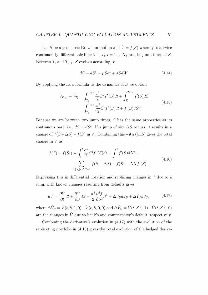
CHAPTER 4. QUANTIFYING VALUATION ADJUSTMENTS 51
Let S be a geometric Brownian motion and V = f(S) where f is a twice
continuously differentiable function. Ti, i = 1 . . . NT are the jump times of S.
Between Ti and Ti+1, S evolves according to
dS = dSc = µSdt+ σSdW. (4.14)
By applying the Ito’s formula to the dynamics of S we obtain
VTi+1− VTi =
∫ Ti+1
Ti
σ2
2S2f ′′(S)dt+
∫ Ti+1
Ti
f ′(S)dS
=
∫ Ti+1
Ti
(σ2
2S2f ′′(S)dt+ f ′(S)dSc).
(4.15)
Because we are between two jump times, S has the same properties as its
continuous part, i.e., dS = dSc. If a jump of size ∆S occurs, it results in a
change of f(S+∆S)−f(S) in V . Combining this with (4.15) gives the total
change in V as
f(S)− f(S0) =
∫ t
0
σ2
2S2f ′′(S)ds+
∫ t
0
f ′(S)dXc+∑0≤s≤t,∆S 6=0
[f(S + ∆S)− f(S)−∆Xf ′(S)].(4.16)
Expressing this in differential notation and replacing changes in f due to a
jump with known changes resulting from defaults gives
dV =∂V
∂tdt+
∂V
∂SdS +
σ2
2
∂2f
∂S2S2 + ∆VBdJB + ∆VCdJC , (4.17)
where ∆VB = V (t, S, 1, 0)−V (t, S, 0, 0) and ∆VC = V (t, S, 0, 1)−V (t, S, 0, 0)
are the changes in V due to bank’s and counterparty’s default, respectively.
Combining the derivative’s evolution in (4.17) with the evolution of the
replicating portfolio in (4.10) gives the total evolution of the hedged deriva-

CHAPTER 4. QUANTIFYING VALUATION ADJUSTMENTS 52
tive
dV + dΠ =(∂V
∂t+σ2
2
∂2V
∂S2S2 + r1α1P1 + r2α2P2+
(rc − qc)αCPC + (γ − q)δS − rxX − γKK)dt+
(α1R1P1 − α1P1 + α2R2P2 − α2P2 + ∆VB)dJB+
(−αCPC + ∆VC)dJC+
(δ +∂V
∂S)dS.
(4.18)
The risks associated with underlying instrument price and counterparty de-
fault can be eliminated by choosing
αCPC = ∆VC , (4.19)
δ = −∂V∂S
. (4.20)
By (i) using the results from (4.19) and (4.20), (ii) denoting the pre-default
bank bond position α1P1+α2P2 with P and the post-default position α1R1P1+
α2R2P2 with PD and (iii) using the funding constraint in (4.11), we can for-
mulate (4.18) as
dV + dΠ =(∂V
∂t+AV − rXX + r1α1P1 + r2α2P2 + λC∆VC − γKK)dt+
(∆VB + V + PD −X)dJB,
(4.21)
where A = σ2
2∂2
∂S2S2 + (qS − γS)S ∂
∂Sand λC = rC − qC .
The zero basis relation in (4.2) and the funding constraint in (4.11) allows
us to write (4.21) as
dV + dΠ =(∂V
∂t+AV − sXX − (r + λB + λC)V+
λCgC + λBgB − εhλB)dt+ εhdJB,
(4.22)

CHAPTER 4. QUANTIFYING VALUATION ADJUSTMENTS 53
where gB = V + ∆VB and gC = V + ∆VC are the post-default values for the
derivative after bank’s and counterparty’s default, respectively, and sX =
rX − r. From the jump term, we can see that in case of the bank’s own
default there is a hedge error of
εh =gB + PD −X − φK
=εh0 + εhK ,(4.23)
where εhK is the capital-dependent part of the error. On the other hand,
unless the bank defaults, it will gain a corresponding incremental cost/gain
of εhλbdt. As long as the bank is alive the combination of the derivative and
hedge portfolio is risk-free.
Let us now assume that, while alive, the bank wants the strategy to
be self-financing and perfectly replicate the derivative value. The direct
implication of this feature is that the drift term in (4.22) must be zero, i.e.,
∂V
∂t+AV − (r + λB + λC)V = sXX − λCgC − λBgB + εhλB + (γK − rφ)K,
(4.24)
with a final condition V (T, S) = H(S), where H(S) is the payoff at maturity.
Recall that V was used for the classic Black-Scholes price of the derivative
whereas V is the value taking into account valuation adjustments. If the
combined valuation adjustment is U , we can write
V = V + U. (4.25)
Because V satisfies the Black-Scholes partial differential equation (PDE)
∂V
∂t+AV − rV = 0, (4.26)
with the final condition V (T, S) = H(S), we can write the following PDE
for the valuation adjustment
∂U
∂t+AU − (r + λB + λC)U =
V λC − gCλC + V λB − gBλB + εHλB + sXX + γKK − rφK,(4.27)
CHAPTER 4. QUANTIFYING VALUATION ADJUSTMENTS 54
with the final condition U(T, S) = 0.
To solve the PDE, we consider Feynman-Kac theorem [Kac, 1951] applied
to the Black-Scholes PDE by Janson and Tysk [2006]. The Feynman-Kac
theorem provides a link between parabolic second order PDEs and stochastic
processes and can be used to solve PDEs by simulating random paths of
a stochastic process. While the approach is used for solving the price of
European call options, it can be extended to solve (4.27) which, for simplicity,
can be written in a more general form
∂U
∂t+AU − κU = ω, (4.28)
with the final condition U(T, S) = 0. According to the Feynman-Kac theo-
rem, the solution for (4.28) can be expressed as the expectation
U = −Et[∫ T
t
e−∫ ut κ(Ss,s)dsω(Su, u)du], (4.29)
which allows us to write the solution for (4.27) as
U = −∫ T
t
e−∫ ut (r(s)+λB(s)+λC(s))dsEt[λC(u)V (u)−
λC(u)gC(V (u), u) + λB(u)V (u)− λB(u)gB(V (u), u)+
λB(u)εh0(u) + sXX(u) + (γK(u)− r(u)φ)K(u) + λBεhK ]du.
(4.30)
By grouping the equation so that we have terms dependent on counterparty’s
credit quality, bank’s credit quality, funding and capital, we can write
U = CV A+DV A+ FV A+KV A, (4.31)
CHAPTER 4. QUANTIFYING VALUATION ADJUSTMENTS 55
where
CV A =−∫ T
t
e−∫ ut r(s)dsλC(u)Et[V (u)− gC(V (u), X(u)]du
DV A =−∫ T
t
e−∫ ut r(s)dsλB(u)Et[V (u)− gB(V (u), X(u)]du
FV A =−∫ T
t
e−∫ ut r(s)ds(λB(u)Et[εh(u)]− r(u)φEt[K(u)]+
sX(u)Et[X(u)])du
KV A =−∫ T
t
e−∫ ut r(s)dsγK(u)Et[K(u)]du,
(4.32)
and r(s) = r(s) + λB(s) + λC(s).

CHAPTER 4. QUANTIFYING VALUATION ADJUSTMENTS 56
4.2 American Monte Carlo algorithm
While most XVAs can be easily approximated via simple numerical integra-
tion techniques, KVA is more complicated due to the capital term K(t) in
the integrand which is usually computed via simulation based techniques. A
simple brute force solution could be applied to solve the nested Monte Carlo
problem, but to enhance computational performance, we consider Ameri-
can Monte Carlo techniques presented by Longstaff and Schwartz [2001].
The method was originally developed for the valuation of American options,
hence the name. American options differ from European options in that the
options can be exercised before maturity. The decision whether or not to
exercise the option must be determined at all times when the option is ex-
ercisable to come up with the optimal exercise strategy and thus a price for
the instrument. The exercise decision at t is done by comparison of the value
from immediate exercise and continuation. The key concept of American
Monte Carlo techniques is to estimate the conditional expectation of pay-
off from continuation by cross-sectional information in the simulation using
least-squares regression, thus removing the need for nested simulations. This
means that, instead of starting a new simulation from each time point in each
path (ω, tk), we estimate the conditional expectation of the option’s value at
(ω, tk) with the information that is provided by all paths ω and available
at tk−1. Valuing American options and calculating KVA are similar in that
both require calculations of conditional expectations at each time step. To
allow for efficient use, we have chosen American Monte Carlo approach for
the calculation of KVA. To formulate the American Monte Carlo algorithm,
we follow the Longstaff and Schwartz [2001] approach closely but apply a few
changes to make it more applicable to our problem.
As in Chapter 3, we assume a finite, discrete and evenly spaced time in-

CHAPTER 4. QUANTIFYING VALUATION ADJUSTMENTS 57
terval [0, T ] with K time steps and a complete probability space (Ω,F ,P),
where Ω is the set of all possible realizations of the stochastic environment
between 0 and T , F is the sigma-algebra, i.e., a closed collection of subsets of
distinguishable events at time T and P is a probability measure on the ele-
ments of F . An augmented filtration of F is an increasing and indexed family
of sub-sigma-algebras of F . It is generated by the instrument price processes
ωi. Let such an augmented filtration be F : F = Ft; t ∈ [0, T ],FT = F. We
assume no arbitrage opportunities, i.e., a risk-neutral measure Q exists for
the stochastic environment. In the original approach, C(ω, s; t, T ) is defined
as the path of cash flows generated by the option given that the option is alive
at t and the optionholder uses optimal exercise strategy for all s, t < s ≤ T .
In other words, C(ω, s; t, T ) represents the payoff received from exercising
the option at some t. The assumption of N discrete time points when the
option is exercisable allows us to write the value of continuation at tk as the
expectation of the discounted cash flows C(ω, s; tk, T )
F (ω; tk) = EQ[N∑
j=k+1
e−∫ tjtkr(ω,s)dsC(ω, tj; tk, T )|Ftk ], (4.33)
where r(ω, s) is the riskless discount rate and the risk-neutral expectation is
taken under Q and conditional on the information set Ftk . Prior to maturity,
the optionholder chooses to exercise the option if the value given by (4.33)
is less than the value from immediate exercise. We will use the notation
C(ω, s; t, T ) for a path of cash flows generated by a generic derivative product,
given that the derivative is alive and if it carries possibilities of exercise,
optimal exercise strategy is used. The value of a derivative without exercise
possibilities is then simply the value of continuation given by (4.33). We also
assume that the generic derivative can be decomposed into sub-components
that generate only one cash flow. For example, interest rate swaps can be
decomposed into a series of consecutive forward rate agreements (FRA), caps

CHAPTER 4. QUANTIFYING VALUATION ADJUSTMENTS 58
into series of caplets, etc.
The conditional expectation F (ω; tk) is an element of a space of square-
integrable functions, i.e., the integral of the square of the absolute value is
finite. Because the space has a countable orthonormal basis, F (ω; tk) can
be presented as a linear combination of a finite set of Ftk-measurable basis
functions. The implication of this assumption is that in the case of valuation
of American options, we can write the value of the option as a function of
the underlying market factors and then approximate the value by regression.
For example, the value of the asset S underlying the option can be used as
the explanatory variable.
After decomposing the derivative contracts into single FRAs, caplets, etc.,
we assume that each future cash flow is dependent on one underlying market
factor. Let the explanatory variable be X(t). We construct the set of basis
functions as simple polynomials of increasing powers of X(t) and write the
linear combination in the general form as
F (ω; tk) =∞∑j=0
ajX(tk−1)j, (4.34)
where the aj coefficients are constants. The basis functions can be easily ex-
panded to take into account multiple underlying market factors by replacing
ajX(tk−1)j with ajX(tk−1)j + bjY (tk−1)j, for example.
Illustrative figures of 1-year interest rates and market values for a re-
ceive floating, pay fixed interest rate swap are shown in Figures 4.3 and 4.4.
The Hull-White model is calibrated with a = 0.2 and σ = 0.015. 1-year
interest rate starts from 3.50%. In the case of a linear derivative product,
such as an interest rate swap, the paths for the underlying interest rate and
the derivative are similar. Figure 4.5 illustrates a simple linear regression
F (ω; tk) = a0 + a1X(tk−1) for the four scenarios when simulated swap values
at tk are regressed onto the basis function at tk−1. First order regression is

CHAPTER 4. QUANTIFYING VALUATION ADJUSTMENTS 59
likely insufficient for options and other products which have more complex
payoff functions.
Let us denote the approximation with the first m <∞ terms as Fm(ω, tk).
Once the basis functions where aj 6= 0 are specified, we start backwards from
maturity tK by estimating Fm(ω, tK−1) with Fm(ω, tK−1) by regressing the
values of cash flows C(ω; s, tK , T ) onto the basis functions for all simulation
paths. By doing this, we construct pairs of derivative values and underlying
market factors (XtK−1, V (XtK )) and estimate the regression parameters aj
from these pairs by minimizing least squares
minaj
(F (ω; tk)− Fm(ω, tk))2. (4.35)
Based on the regression coefficients, we can estimate the conditional ex-
pectation of the derivative’s value when we know the underlying market
factor in each scenario. It can be shown that the fitted regression value
Fm(ω, tk) converges in probability and in mean square as the number of
simulation paths approaches infinity [White, 1984]. Also, Theorem 1.2.1 of
Amemiya [1985] implies that the estimate is the best linear mean-squared
metric based unbiased estimator of Fm(ω, tk). The fitted regression value
Fm(ω, tK−1) represents the expected value of the derivative at tK−1 for path
ω. We then continue stepwise by estimating Fm(ω, tK−i), i = 2, . . . by regress-
ing the values of C(ω; s, tK−1, T ) onto the basis functions at tK−2, values of
C(ω; s, tK−2, T ) onto the basis functions at tK−3 and so on. By averaging
over all paths, we obtain an expected exposure (EE) profile for the deriva-
tive. Providing a general convergence rule for the algorithm may be difficult
as the number of time points, basis functions and paths go to infinity unless
certain limits are set.

CHAPTER 4. QUANTIFYING VALUATION ADJUSTMENTS 60
Figure 4.3: Interest rate swap market value development in four randomly
chosen scenarios. The Hull-White short rate model is calibrated with a =
0.2 and σ = 0.015. Time points in the x-axis represent days.
Figure 4.4: 1-year interest rate development in four illustrative scenarios.
The 1-year interest rate is 3.50% at t = 0 and the Hull-White short rate
model is calibrated with a = 0.2 and σ = 0.015. Time points in the x-axis
represent days.

CHAPTER 4. QUANTIFYING VALUATION ADJUSTMENTS 61
Figure 4.5: Linear regression of swap values at t onto the basis function at
t− 1
4.3 Capital valuation adjustment for regula-
tory default risk charge
After the general representation of the algorithm, we now consider the default
risk capital requirement K(tk) for a portfolio of derivatives shown in (3.41)
and substitute EAD to EE using (3.7) and (3.6)
K(tk) = RW · 8% · α ·∫ T
t=tk
max (EE(tk), . . . , EE(t))dt, (4.36)
where the risk weight RW is assumed to be constant, T is either the one-year
point or the maturity of the longest dated contract if all the contracts mature
within a year.
For the modeling of the EE profile, we re-consider the pseudo-algorithm
in Chapter 3.2.1.2. We start by generating M market scenario paths for all

CHAPTER 4. QUANTIFYING VALUATION ADJUSTMENTS 62
underlying market factors Xi. Specifically, interest rates are generated with
the Hull-White model presented by Hull and White [1990]
dr(t) = (θ(t)− ar(t))dt+ σdW (t), (4.37)
and FX rates with geometric Brownian motion
dS(t) = µS(t)dt+ σS(t)dW (t). (4.38)
We decompose all derivatives into sub-components that generate only one
cash flow. After obtaining the cash flows C(ω; s, tK , T ) generated by each
derivative at maturity tK , we use the basis functions and least-squares re-
gression to obtain conditional expectations Fm(ω, tK−1) for each derivative’s
value at tK−1 conditional on the information set at tK−1. As each deriva-
tive’s value is now dependent only on one discounted cash flow, the relevant
explanatory variables are trivial. For example, in the case of an interest rate
product, such as a floating for fixed FRA, the underlying floating interest rate
is the only explanatory variable. In this case, we use the underlying interest
rate at tK−1 as an explanatory variable and construct pairs of those and the
FRA’s values at tK for each simulation path. By considering all simulation
paths, we can then find the optimal regression parameters and estimate the
conditional expectation of the FRA’s price using only the underlying inter-
est rate at tK−1. By starting from maturity and continuing backwards until
the current time point, this makes it possible to approximate an individual
trade’s expected exposure for each time point.
We use F im(ω, tk) to denote the estimate for derivative i’s market value at
tk in path ω obtained by recursively generating the conditional expectations
via fitted regression. An estimate for portfolio level EE profile at tk is then
obtained by averaging over the estimated positive portfolio-level realizations
EE(tk) ≈1
Mpos
∑ω
[n∑i=1
F im(ω, tk)]
+, (4.39)

CHAPTER 4. QUANTIFYING VALUATION ADJUSTMENTS 63
where Mpos is the number of positive portfolio-level realizations at tk. EEPE
is calculated by using the trapezoidal rule for numerical integration of the
non-decreasing EE curve
EEPE(tk) =J∑j=1
E(tk, j − 1) + E(tk, j)
2(tk+j − tk), (4.40)
where E(tk, j) = max (EE(tk), . . . , EE(tk + j)) is the non-decreasing EE
curve and tk+J = T .
The expected capital requirement Et[K(tk)] needed to solve KVA in (4.32)
is approximated with K(tk)
K(tk) = RW · 8% · α · EEPE(tk). (4.41)
By using this, we can solve KVA at tk from
KV A =−∫ T
tk
e−∫ ut r(s)dsγK(u)Et[K(tk)]du. (4.42)
by using the trapezoidal rule and the approximation Et[K(tk)] ≈ K(tk)
KV A(tk) =J∑j=1
K(tk, j − 1) +K(tk, j)
2(tk+j − tk)γK(tk+j+1), (4.43)
where rtk+j is the discount rate from tk to tk+j and K(tk, j) = e−rtk+j K(tk+j)
is the discounted capital charge at tk+j.

Chapter 5
Numerical examples
We demonstrate the model for estimating KVA with an interest rate swap
between a bank and a counterparty.
5.1 Setting and assumptions
We assume a situation between a bank and a counterparty which (i) is an
investment grade company with a risk weight of 0.3 and (ii) does not have a
credit support annex (CSA). The parties have entered into an interest rate
swap. The bank has an annual total capital cost of γK = 10% and uses
the regulatory scaling factor α = 1.4 for EAD. We use Actual/365 date
convention and linear regression to obtain interest rates between two tenors
in the yield curve. The Hull-White interest rate model
dr(t) = (θ(t)− ar(t))dt+ σdW (t) (5.1)
is calibrated with mean reversion rate a = 0.24 and volatility parameter
σ = 0.015. See Gurrieri et al. [2009] for a comprehensive framework of
calibrating the Hull-White model parameters. The yield curve at t = 0 is
shown in Figure 5.1. Each simulation is run with 1000 scenarios and one
64

CHAPTER 5. NUMERICAL EXAMPLES 65
Figure 5.1: Yield curve at base date
time step represents one day. We determine the capital costs the bank needs
to incorporate in the valuation of the interest rate swap.
5.2 Capital valuation adjustment for an at-
the-money interest rate swap
The counterparty has agreed on paying floating rate to the bank in exchange
for fixed 3.95 % on a notional of 10000 units in the domestic currency for 10
years. Details are shown in Table 5.1.
The evolution of 1-year interest rates is shown in Figure 5.2. The evolu-
tion of the full yield curve for a randomly chosen scenario is in Figure 5.3.

CHAPTER 5. NUMERICAL EXAMPLES 66
Figure 5.2: 1-year interest rates evolution in 1000 scenarios for each simula-
tion time point during the 10 years lifetime of the trade. 1-year interest rate
is 3.50% at t = 0 and the Hull-White short rate model is calibrated with a
= 0.2 and σ = 0.015.
Figure 5.3: Full yield curve evolution in a randomly chosen scenario. 1-
year interest rate is 3.50% at t = 0 and the Hull-White short rate model is
calibrated with a = 0.2 and σ = 0.015.

CHAPTER 5. NUMERICAL EXAMPLES 67
Table 5.1: Details of the at-the-money interest rate swap
Swap Notional Tenor (years) Pay leg rate Receive leg rate
1 10000 10 Fixed 3.95% Floating
Figure 5.4: Simulated FRA market values in a randomly chosen scenario.
The Hull-White short rate model is calibrated with a = 0.2 and σ = 0.015.
Figure 5.4 illustrates how the swap is decomposed into single FRAs which
mature every time the swap is fixed. Figure 5.5 shows the simulated market
values for the interest rate swap.
For each simulation date, the instantaneous forward rate until the matu-
rity of the FRA is used an an explanatory variable for the regression. The
regressed market values for the swap are in Figure 5.6. We use linear regres-
sion
F (ω; tk) = a0 + a1X(tk−1), (5.2)
where X(t) is the instantaneous forward rate until the maturity of the FRA
and a0, a1 are constants. Parameters are estimated by the least-squares
approach. The regressed values for each simulation date and scenario are

CHAPTER 5. NUMERICAL EXAMPLES 68
Figure 5.5: Simulated swap market values from t = 0 to t = 10(years) in
1000 scenarios.
Figure 5.6: Estimated swap market values from t = 0 to t = 10(years) in
1000 scenarios. Simulated market values are explained with Y = a+ bx,

CHAPTER 5. NUMERICAL EXAMPLES 69
shown against the simulated values in Figure 5.7. The EE profile for the
swap is shown in Figure 5.8.
The spot capital charge for all simulation dates is shown in 5.9. The
numerical integration techniques discussed Chapter 4 give KV A ≈ −17 units
or -17bp of the swap’s notional. This means that in order to cover the
capital costs resulting from entering into the swap, the bank must offer the
counterparty such a fixed rate, that right after inception the market value
is +17 - and this is only for the default risk capital charge. The result is of
similar magnitude to the results in Green et al. [2014]. The 10-year credit
default swap (CDS) spreads for sovereigns from January 2006 to September
2008 were between 19.70bp and 73.20bp [European Central Bank, 2010].
Typical CDS spreads for investment grade companies in August 2017 ranged
from 80.01bp (industrials) to 211.15bp (high volatility) [Markit, 2017]. By
comparing the magnitude of KVA to the typical credit-based premia, is it
clear that the impact having to hold regulatory capital should be considered
in OTC derivatives pricing.
According to empirical experiments, the results are sensitive to the se-
lection of the volatility parameter σ in the Hull-White model. For example,
using σ = 0.15 gives KV A ≈ −143. However, the realizations for even the
shortest rate reached levels above 20%, which does not seem reasonable given
the development of Libor rates during the past 30 years [Macrotrends, 2017].
The spot capital profile with σ = 0.15 is shown in Figure 5.10.
Due to the selection of the American Monte Carlo algorithm, the com-
putation time for the selected settings was approximately 5 seconds with a
normal PC, which makes it very likely that the computational performance
of the model is sufficient for pricing purposes.

CHAPTER 5. NUMERICAL EXAMPLES 70
Figure 5.7: Fitted regression of swap market values
Figure 5.8: Expected exposure for the 10 year lifetime of the trade
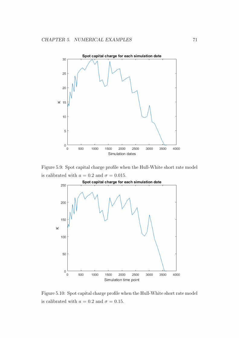
CHAPTER 5. NUMERICAL EXAMPLES 71
Figure 5.9: Spot capital charge profile when the Hull-White short rate model
is calibrated with a = 0.2 and σ = 0.015.
Figure 5.10: Spot capital charge profile when the Hull-White short rate model
is calibrated with a = 0.2 and σ = 0.15.
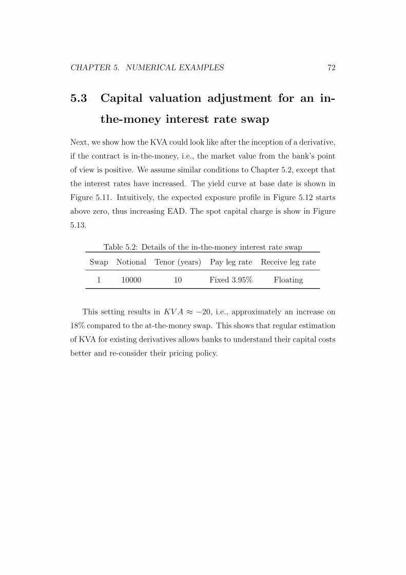
CHAPTER 5. NUMERICAL EXAMPLES 72
5.3 Capital valuation adjustment for an in-
the-money interest rate swap
Next, we show how the KVA could look like after the inception of a derivative,
if the contract is in-the-money, i.e., the market value from the bank’s point
of view is positive. We assume similar conditions to Chapter 5.2, except that
the interest rates have increased. The yield curve at base date is shown in
Figure 5.11. Intuitively, the expected exposure profile in Figure 5.12 starts
above zero, thus increasing EAD. The spot capital charge is show in Figure
5.13.
Table 5.2: Details of the in-the-money interest rate swap
Swap Notional Tenor (years) Pay leg rate Receive leg rate
1 10000 10 Fixed 3.95% Floating
This setting results in KV A ≈ −20, i.e., approximately an increase on
18% compared to the at-the-money swap. This shows that regular estimation
of KVA for existing derivatives allows banks to understand their capital costs
better and re-consider their pricing policy.
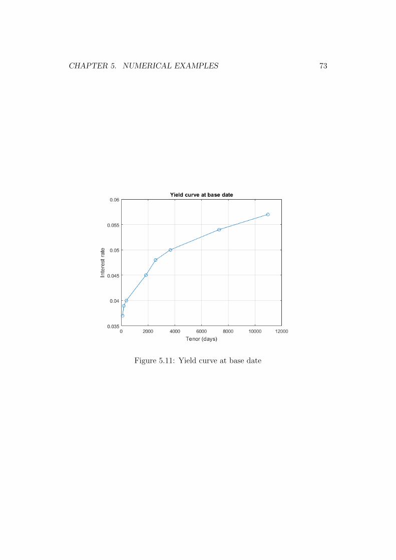
CHAPTER 5. NUMERICAL EXAMPLES 73
Figure 5.11: Yield curve at base date

CHAPTER 5. NUMERICAL EXAMPLES 74
Figure 5.12: Expected exposure profile for the in-the-money swap when the
Hull-White short rate model is calibrated with a = 0.2 and σ = 0.015.
Figure 5.13: Spot capital charge profile for the in-the-money swap when the
Hull-White short rate model is calibrated with a = 0.2 and σ = 0.15.

Chapter 6
Conclusions
The purpose of this study was to develop a method which can be used by
a bank to incorporate cost of having to hold regulatory capital into over-
the-counter (OTC) derivatives pricing. This capital valuation adjustment
is known as KVA. We assumed that the bank has an approval for inter-
nal model method (IMM), and limited this study to regulatory default risk
capital charge, which is calculated using simulation-based techniques.
First, we introduced the risks related to OTC derivatives and what miti-
gating actions banks may take to reduce them. Next, we introduced the key
counterparty credit risk measures, i.e., current exposure (CE), probability
of default (PD), loss given default (LGD), exposure at default (EAD), risk
weight (RW) and risk weighted assets (RWA) and how they are translated
into a regulatory capital requirement. Finally, we summarized the most com-
mon and important valuation adjustments to account for both parties’ credit
qualities, funding and capital in OTC derivatives pricing. We concluded that
the classic Black-Scholes price for a derivative is problematic. This makes
it increasingly important to incorporate credit valuation adjustment (CVA),
debt valuation adjustment (DVA), funding valuation adjustment (FVA) and
capital valuation adjustment (KVA) into OTC derivatives pricing in the en-
75

CHAPTER 6. CONCLUSIONS 76
vironment of tightening regulation.
Then, we formulated a model that uses stochastic scenario generation to
produce expected exposure (EE) curve for a portfolio of OTC derivatives and
makes it possible to calculate exposure-at-default (EAD) for the portfolio.
Together with regulatory risk weights and capital ratios, this gives the capital
charge for default risk. Also, we briefly discussed other capital charges banks
have to consider.
By extending the methods of Burgard and Kjaer [2013] and Green et al.
[2014], we constructed a replicating portfolio for an OTC derivative which
made it possible to derive an expression for KVA under the IMM methodology
for regulatory default risk capital charge. While the problem could have
been solved with brute force, to improve computational performance, we
used American Monte Carlo techniques to calculate KVA. The selection of
this method was critical in preserving the possibility to use the KVA model
for pricing purposes.
Finally, we determined KVA for illustrative interest rate swaps. The
results show that neglecting the cost of capital - even for only default risk -
can lead to mispricing. In addition, a bank which considers other valuation
adjustments, such as CVA, DVA, FVA and KVA for other capital charges,
as well as operative costs, may have to charge a significant premium for
a counterparty to make an OTC derivative profitable. Due to the careful
selection of the simulation algorithm, the model’s computational performance
was sufficient for pricing.
Topics for further research include the modeling of KVA for other capital
charges, primarily market risk charge and CVA risk charge. Also, the optimal
choice of basis functions in the regression is left for further study. Possible
basis functions for non-linear products include Hermite, Laguerre and Jacobi
polynomials.
Bibliography
1. T. Amemiya. Advanced Econometrics. Harvard University Press,
1985.
2. Bank for International Settlements. Exchange-traded derivatives
statistics. BIS, September, 2016a.
3. Bank for International Settlements. Semiannual OTC derivatives
statistics. BIS, September, 2016b.
4. Bank for International Settlements. Basel committee charter.
https://www.bis.org/bcbs/charter.htm, 2016c.
5. Basel Committee on Banking Supervision. An explanatory note on
the Basel II IRB risk weight functions, 2005a.
6. Basel Committee on Banking Supervision. The application of Basel
II to trading activities and the treatment of double default effects.
BCBS-116, 2005b.
7. Basel Committee on Banking Supervision. International convergence
of capital measurement and capital standards. BCBS-128, 2006.
8. Basel Committee on Banking Supervision. Basel III: A global regula-
tory framework for more resilient banks and banking systems. BCBS-
189, 2010.
77

BIBLIOGRAPHY 78
9. Basel Committee on Banking Supervision. Capital requirements for
bank exposures to central counterparties. BCBS-227, 2012.
10. Basel Committee on Banking Supervision. The non-internal model
method for capitalising counterparty credit risk exposures. BCBS-
254, 2013a.
11. Basel Committee on Banking Supervision. Review of the credit valu-
ation adjustment risk framework. BCBS-254, 2013b.
12. Basel Committee on Banking Supervision. Framework for supervisory
stress testing of central counterparties (CCPs), 2017.
13. N. H. Bingham. Springer: Risk-Neutral Valuation: Pricing and Hedg-
ing of Financial Derivatives, 2004.
14. F. Black and M. Scholes. The pricing of options and corporate liabil-
ities. Journal of Political Economy, 3, pp. 637-654, 1973.
15. C. Burgard and M. Kjaer. Partial differential equation representations
of derivatives with bilateral counterparty risk and funding costs. The
Journal of Credit Risk, 7 (13), pp. 1-19, 2010.
16. C. Burgard and M. Kjaer. Funding strategies, funding costs. Risk,
December, 2013.
17. A. Carol. Market Risk Analysis, Value at Risk Models. John Wiley
and Sons, 2009.
18. R. Cont and P. Tankov. Financial Modelling with Jump Processes.
Chapman and Hall/CRC Financial Mathematics Series, 2004.
19. J.C. Cox, J.E. Ingersoll, and S.A. Ross. A theory of the term structure
of interest rates. Econometrica, 53 (2), pp. 385-407, 1985.

BIBLIOGRAPHY 79
20. D. Duffie and K. J. Singleton. Credit Risk: Pricing, Measurement,
and Management. Princeton Series in Finance, 2003.
21. D. Duffie and H. Zhu. Does a central clearing counterparty reduce
counterparty risk? The Review of Asset Pricing Studies, 1 (1), pp.
74-95, 2011.
22. B. Engelmann and R. Rauhmeier. The Basel II Risk Parameters.
Springer, 2006.
23. European Central Bank. An analysis of euro area sovereign CDS and
their relation with government bond. Working paper series, 1271,
2010.
24. S. Ghamami and B. Zhang. Efficient Monte Carlo counterparty credit
risk pricing and measurement. The Journal of Credit Risk, 10 (3), pp.
87-133, 2014.
25. A. Green. XVA: Credit, Funding and Capital Valuation Adjustments.
John Wiley and Sons, 2015.
26. A. Green, C. Kenyon, and C. Dennis. KVA: Capital valuation adjust-
ment. Risk, December, 2014.
27. J. Gregory. Counterparty Credit Risk and Credit Value Adjustment:
A Continuing Challenge for Financial Markets. John Wiley and Sons,
2012.
28. J. Gregory. The XVA Challenge: Counterparty Credit Risk, Funding,
Collateral and Capital, 3. John Wiley and Sons, 2014.
29. S. Gurrieri, M. Nakabayashi, and T. Wong. Calibration methods of
Hull-White model. SSRN eLibrary, 2009.

BIBLIOGRAPHY 80
30. D. Heath, R. Jarrow, and A. Morton. Bond pricing and the term
structure of interest rates: A discrete time approximation. Journal of
Financial and Quantitative Analysis, 25 (4), pp. 419-440, 1990.
31. J. Hull. Options, Futures and Other Derivatives. Pearson Education,
Inc., 1988.
32. J. Hull and A. White. Pricing interest-rate-derivative securities. The
Review of Financial Studies, 3 (4), pp. 573-592, 1990.
33. J. Hull and A. White. Bond option pricing based on a model for the
evolution of bond prices. Advances in Futures and Options Research,
6, pp. 1-13, 1993.
34. J. Hull and A. White. The FVA debate. Risk, July, 2012.
35. International Swaps and Derivatives Association. Overview of ISDA
standard credit support annex (SCSA). ISDA, November, 2011.
36. International Swaps and Derivatives Association. ISDA margin survey.
August, 2015.
37. International Swaps and Derivatives Association. Benefits of close-out
netting of derivative transactions. ISDA, June, 2016.
38. N. Iqbal and S. A. Ali. Estimation of probability of defaults (PD)
for low default portfolios: An actuarial approach. ERM Symposium,
2012.
39. S. Janson and J. Tysk. Feynman-Kac formula for Black-Scholes type
operators. Bulletin of the London Mathematical Society, 38 (2), pp.
269-282, 2006.

BIBLIOGRAPHY 81
40. M. Kac. On some connections between probability theory and dif-
ferential and integral equations. Proceedings of the Second Berkeley
Symposium on Mathematical Statistics and Probability, University of
California Press, pp. 189-215, 1951.
41. F. A. Longstaff and E. S. Schwartz. Valuing American options by
simulation: A simple least-squares approach. The Review of Financial
Studies, 14 (1), pp. 113-147, 2001.
42. Macrotrends. Libor rates - 30 year historical chart.
http://www.macrotrends.net/1433/historical-libor-rates-chart,
2017.
43. Markit. CDS bond basis indices. http://www.markit.com/markit.jsp,
2017.
44. A. Pallavicini, D. Perini, and D. Brigo. Funding valuation adjustment:
a consistent framework including CVA, DVA, collateral, netting rules
and re-hypothecation. SSRN eLibrary, 2011.
45. A. Pykhtin and S. Zhu. ”Measuring counterparty credit risk for trad-
ing products under Basel II” in The Basel Handbook . Risk Books,
2006.
46. T. Schuermann. What do we know about loss given default. Federal
Reserve Bank of New York, Working paper, 2004.
47. A. R. Sorkin. Too Big to Fail: The Inside Story of How Wall Street and
Washington Fought to Save the Financial System - and Themselves.
Penguin Books, 2009.
48. O. Vasicek. An equilibrium characterization of the term structure.
Financial Economics, 5 (2), pp. 177-188, 1977.

BIBLIOGRAPHY 82
49. H. White. Asymptotic Theory for Econometricians. Academic Press,
New York, 1984.
50. P. Wilmott. Paul Wilmott Introduces Quantitative Finance. John
Wiley and Sons, 2001.