1

Pricing derivatives if trading in the underlying is limited: Froot and Stein, and Merton ‘98

As one of various suggested applications of their model, Froot and Stein describe the pricing of

derivatives on assets that are not (cost-effectively) tradable.1 They derive a partial differential equation

for the value a bank would assign to an option on an asset that cannot be traded easily (e.g. due to lack

of liquidity or short-selling constraints), but for which observable market prices are available. The

derivation is as follows:

The bank assumes that the observable market price S of the underlying nontraded asset (e.g. an illiquid

share of a common stock) follows a geometric Brownian motion (lognormal diffusion process) with drift

(instantaneous expected return) μS and volatility σS:

SdzSdtdS s

As the price of the untraded asset is observable (and consistent with the assumed pricing model for

tradable assets), the option price is a continuous and twice differentiable function of time t and the

underlying asset price2, so Ito’s lemma3 can be applied on this process – and subsequent taking of

expectations gives an expression for the expected change of the option value F:

1 page 73 in: Risk Management, Capital Budgeting, and Capital Structure Policy for Financial Institutions: An Integrated

Approach, Kenneth A. Froot and Jeremy C. Stein, The Journal of Financial Economics, 1998, no. 47, 55-82. 2 That the option value is a twice differentiable function of underlying price and time (and hence Ito’s lemma is applicable) is a

derived conclusion – the derivation for traded assets is given in Robert C. Merton ’77 – On the Pricing of Contingent Claims and

the Modigliani Miller Theorem, Journal of Financial Economics, Vol. 5, 1977, p. 241-249. If trading in the underlying is not

possible, Merton argues in Applications of Option Pricing Theory: 25 Years Later, American Economic Review, Vol. 88, Issue 3,

June 1998, p. 323 – 349, that one can still define a derivative value function as if the underlying was tradable, and a hedging

strategy that approximates this function by dynamically allocating funds between a portfolio of tradable risky assets to track

the underlying, and the riskless asset. For the hedging strategy that approximates the derivative value function best, the

weights of the assets in the tracking portfolio are chosen so that the variance of the instantaneous tracking error, i.e. the

difference between the instantaneous return of the tracking portfolio and the untradeable asset, is minimized. This implies

that the instantaneous tracking error is uncorrelated with any traded asset’s instantaneous return, as Merton has shown in his

book Continuous Time Finance – in the revised edition of this book the proof can be found on page 396 within the section on

theorem 15.3. An alternative proof is given below, see pages 5-6. It follows that the tracking error is also uncorrelated with the

market portfolio (or any priced factor), and therefore, Merton states, on markets where only systematic risk is priced (as under

the Froot and Stein pricing model assumption for traded assets used here – see the earlier posts in this blog and references

given there for details), the price of the derivative will be the same as if the underlying asset was traded – see Merton ’98, page

333. For additional, informal intuition why this is the case, note that with continuous rebalancing, the probability distribution

of the underlying return over any instantaneous period is the same as the probability distribution of the tracking portfolio

return minus the tracking error. The underlying can hence be replicated with the tracking portfolio minus an additional random

payment series corresponding to the tracking error at the end of each instantaneous period – which as the latter constitutes

only non-systematic risk, and as it does not require cash outlay at the beginning of the period, has an expected value of zero,

and a volatility such that the variance of the tracking portfolio plus the variance of these payments to match the tracking error

equal the untradeable underlying’s variance. And with a replication strategy for the underlying found in this manner, the

conditions for the application of Ito’s lemma are met as well as in the case with observable prices.

3 See the appendix A.1 on Ito’s Lemma.

2

I. tSS

F

t

FSE

S

FFE

22

2

2

2

1

In return notation, the Froot and Stein hurdle rate for a new, small exposure is:4

II. NpRNMN Gr *

With GR corresponding to the Rubinstein measure of relative risk aversion for the bank5, pNNp rr ,cov

being the covariance of the return of the untradeable component of the new investment with the return

of the existing portfolio of untradeable assets, MNNM rr ,cov the covariance of the new investment’s

return with the priced market factor, r the riskless interest rate, the market price of risk and *N the

expected return required by the bank for a small investment into the new untradeable asset.6

Accordingly, the instantaneous hurdle rate *F for an option with price F can be written as follows (with

r now being expressed as annual rate with continuous compounding, and t with unit years):

FpRFMpRMF GtrrF

FGr

F

Ftr

,cov,cov*

The change of the option value and hence the option return is a function of the instantaneous return of

the underlying stock rS:7

SS

SSSS

rF

SF

F

F

SrFS

SSFSFF

And therefore both the covariance of the option with the market and its covariance with the

untradeable part of the existing portfolio ( FM and Fp ) can be expressed as functions of the respective

covariance parameters of the underlying stock ( SM and Sp ):

SpRSMSF GF

SFtr *

4 For notes on the derivation of this hurdle rate see the October ’14 post in this blog and the references given there – note that

the rate here is before subtracting financing costs (risk free rate). 5 This is based on interpreting the payoff function of the bank’s future, non-stochastic investment opportunity after deducting

financing cost as utility function – for details see the October and November 14 posts on the Froot-Stein model in this blog, and the references given there (note that in the previous posts GR was labelled GK ). 6 As the market price of the stock is consistent with the pricing model for traded assets, sMs r and the bank would

not pay the observable “market price” for the not perfectly tradable stock (unless 0Np ), but would require a discount (or

be willing to pay a premium, depending on the sign of Np ) – see Froot and Stein page 73 (note that the variance of the

untradeable component does not appear here, as for a small investment, the impact on portfolio variance due to the asset’s stand-alone variance is considered to be negligible – different to the potential covariance impact). 7 see again fn. 2

3

And with equation II., one can write this hurdle rate as a function of the (minimum) expected stock

return *S the bank would require if it had to hold the stock directly:

trF

SFtr SSF **

*F is the fair (required) instantaneous expected return of the option from the bank’s perspective.

Multiplying with the option value gives the required instantaneous expected change of the option value:

III.

tr

F

SFtrFF SSF

**

And as the expected change of the value of the option is also given by I., if the option is priced fairly

from the bank’s perspective equation I. and III. are equal:8

IV. tSFFSFtrSFtFr SStSSS

22*

2

1

Slightly rearrange IV.:

tSFFtrSFtFr SStSS

22*

2

1

and with SSS ** :

tSFFtrSFtFr SStSS

22*

2

1

Further rearranging gives equation 17 in Froot and Stein:

02

1 22*

trFFSFSFtr SStSS

Rearranging again:

02

1 *22 trFtFFStrStFS tSSSS

And with *S now also expressed as annualized figure (and hence multiplied with t ):

02

1 *22 trFtFFtStrStFS tSSSS

8 The same principle as for the alternative derivation of their option value differential equation by Black and Scholes (see the

appendix A.2 and the earlier post in this blog on that derivation) is applied here – the expected change of the option value derived with Ito’s lemma is compared to the expected change of the value required by the investor – while in Black-Scholes the required expected change is the market’s required expected change determined with the CAPM, here an additional component is included by the bank to compensate for the impact of the bank’s portfolio’s untraded risk.

4

Now divide the whole equation by t :

02

1 *22 rFFFSrSFS tSSSS

This is essentially the differential equation given by Merton for European options on stocks paying a

constant dividend yield *S .9 Hence the corresponding option pricing formulas can be applied to

calculate a fair price from the bank’s perspective, by setting the constant continuous dividend yield

equal to *S . These formulas for stocks paying a constant dividend yield lead to the same result as

discounting the stock price with the dividend yield, and then applying the corresponding Black-Scholes-

Merton formula for a European option on a non-dividend paying stock, with this discounted stock price

(and a slightly modified volatility measure), i.e. by setting the underlying spot price for the option

valuation to:10

TSeS*

0

An intuitive reason for this equivalence is that after discounting the price of the dividend paying stock

with the certain dividend yield (and adjusting the volatility), the probability distribution of that stock

price at T will be the same as the probability distribution for the price at T of an (otherwise equal) non-

dividend-paying stock with current price equal to that discounted price.11

Pricing derivatives on untraded assets if prices are not continuously observable

Merton’s reasoning for pricing an option on an untradeable asset, when its price is only observable at

the time the option is written and its expiry date, is based on the approach with observable prices

described above in footnote 2. As in the case with observable prices, if the underlying is not traded, a

portfolio of traded assets can be used to track the underlying’s return as closely as possible. The return

of the underlying in an instantaneous interval is the difference of this tracking portfolio’s return and the

9 See Robert C. Merton, Theory of Rational Option Pricing, The Bell Journal of Economics and Management Science, Vol. 4, No. 1

(Spring, 1973),pp. 141-183, equation 44 and Footnote 62, p.171. The option pricing formula given there implies that the dividend rate is a riskless instantaneous rate, paid in every infinitesimal small time interval during the life of the option. An explicit derivation for this special case can be found in John C. Hull, Options, Futures & Other Derivatives, Ninth edition (in the following referred to as “Hull”, p. 372). Hull further shows, that the put call parity also holds for options on stocks paying a constant dividend yield and derives the valuation formula for a put on a dividend paying stock (Hull p.372/373 and technical note 6, http://www-2.rotman.utoronto.ca/~hull/TechnicalNotes/TechnicalNote6.pdf). Note that instead of the partial derivative of the option price with respect to the current time variable t, Merton uses the partial derivative with respect to time till expiration – which leads to the different sign of that partial derivative in Merton ‘73. 10

Hull, p. 372. the volatility measure has to be adjusted, as with a lower stock price a given price change is relatively larger (Hull p.343 fn. 12 – note that the adjustment is labelled there as “approximation” as it is introduced in the more general context with dividends not necessarily being paid with a constant yield – however for the special case with a constant instantaneous dividend yield like here, this approximation is exact). 11

Ibid. “having the same probability distribution” can here be interpreted as “having the same value in every state of the world”. Further, recall that the additional return component required by the bank in Froot and Stein can be interpreted as a discount (or potential premium, in case of a negative covariance of the position with the existing portfolio of untradeable assets) on the stock price. see again fn. 6 and the reference given there.

5

tracking error (with the tracking error defined as the difference between instantaneous tracking

portfolio return and instantaneous underlying return). With prices being only observable at issue and

expiry date of the option, during the life of the option the value of the tracking portfolio constitutes the

best estimate of the value of the underlying. The instantaneous tracking errors are unobservable, and

cumulate to a total tracking error that becomes only visible at option expiry. At this moment the true

value of the underlying gets revealed and the best estimate jumps from the value of the tracking

portfolio to the true value.12 This means that the underlying asset price can be modelled as a special

case of a mixed-jump diffusion process – more details further below.

To derive the properties of the tracking portfolio mentioned in footnote 2, note that the instantaneous

return rs of a tracking portfolio consisting of positions in all tradable assets i,…,n with portfolio weights

wi is given by:

n

i

iis rwr

1

With the instantaneous return of the untradeable asset labelled vr , the instantaneous tracking error x is

defined as follows:

v

n

i

iivs rrwrrx 1

The expected instantaneous tracking error is therefore:

v

n

i

iiv

n

i

iivsxx wrrwErrErE

11

and the variance of the instantaneous tracking error:

n

i

ivi

n

i

v

n

ji

ijjivsvsx www

11

2222 22

The tracking portfolio is supposed to track the underlying return as closely as possible, i.e. the variance

of the tracking error is minimized, which gives the following set of conditions:

022

1

2

iv

n

j

ijji

x ww

12

Merton ’98, p. 335

6

ivis

iv

n

j

ijjw

1

I.e., when the tracking variance is minimized, the covariance of the tracking portfolio with any tradable

asset equals the covariance of the untradeable underlying with that tradable asset.

It follows for the covariance of the tracking error of the optimal tracking portfolio with any tradable

asset:

0

1

iv

n

j

ijjix w

Therefore, the tracking error is uncorrelated with the tracking portfolio, and hence:

222vxs

Or with annualized instantaneous variances dt:

dtdtdt vxs222

Merton assumes that the tracking error is normally distributed.13 Further, the replication portfolio is

rebalanced continuously, and all assets’ volatilities and expected returns are constant, so the volatility

and expected value of the tracking error are constant.14 The instantaneous tracking error can therefore

be represented by a stochastic differential equation for a variable X (with an arbitrary starting value X0):

xxx XdzXdtdX

such that x=dX/X is the instantaneous tracking error and with xz being a Wiener process. Merton

assumes a starting value of X0=1. Xt then can be interpreted as the value per notional dollar of a

portfolio which in t=0 consists of a long position in the tracking portfolio “financed” with a short position

with equal notional size in the untradeable asset. Merton refers to Xt as cumulative proportional

tracking error.

As assets are jointly normal15, and if no dividends are assumed, the process assumed by Merton for the

tracking portfolio of traded assets can be written as follows:

13

See the process for the tracking error in Merton ’98, p. 330, where the stochastic component contains a Wiener process. 14

This follows from Merton ‘98, page 330 where it says that at each point in time, the weights in the replicating portfolio are chosen as to minimize the tracking error variance, and the assumption that the instantaneous covariance matrix including the asset to be hedged and all traded assets stays constant over time. 15

Merton does not explicitly state this assumption, however, tracking error and underlying are normally distributed and uncorrelated, and the sum of two uncorrelated normal variables is also normal – so to ensure that this holds here, the returns of the traded assets and the untraded asset must be jointly normal.

7

sss SdzSdtdS

With zS being a Wiener process (this is essentially equation 4 in Merton ’98, here adjusted for zero

dividends). The instantaneous return of the tracking portfolio is hence:

SSSs dzdtS

dSr

The untraded asset follows a similar process – see assumption 2 in Merton ’98, again here adjusted for

the case of zero dividends:

vvv VdzVdtdV

with vz being a Wiener process. Hence, the instantaneous return of the untraded asset (which is

unobservable) equals:

vvvv dzdtV

dVr

With the process for S shown above, the value of S at the option’s expiry date, ST, can be (somewhat

informally) written as follows:16

N

ttsdzsTs

s

eSST1

,2

2

0

Where the period T is divided into infinitesimal small time intervals with length dt, numbered from 1 till

N.

And correspondingly VT and XT can be expressed as:

N

ttvzvTv

v

eVVT1,

2

2

0

and:

N

ttxzxTx

x

eXXT1,

2

2

0

The instantaneous tracking error is the difference of the instantaneous returns of the replication

portfolio and the untradeable asset:

VVVSSSXXX dzdtdzdtV

dV

S

dSdzdt

X

dX

16

See the section on the stock price after a period longer than dt in the appendix A.1 on Ito’s Lemma.

8

As Merton argues, if the CAPM (or another equilibrium model that implies that the market prices only

systematic risk) holds and as the tracking error is uncorrelated with any tradable asset and hence the

market portfolio (or priced factor), i.e. the tracking error is purely nonsystematic, then the

instantaneous expected returns of untradeable asset and replication portfolio are equal and the

expected instantaneous tracking error is zero.

Substituting 0X in the equation above for XT :

N

ttxdzxTx

eXXT1

,2

2

0

As X0 = 1:

N

ttxdzxTx

eXT1

,2

2

And hence:

N

ttxdzx

N

ttsdzsTxs

s

N

ttxdzxTx

N

ttsdzsTs

s

eS

eeS

XS TT

1,

1,

2

22

1,

2

2

1,

2

2

0

0

And with

222vxs , dtdt vs and xxssvv dzdzdz

This simplifies to:

N

ttvdzvTv

v

eSXS TT

1,

2

2

0

Because V0=S0:

TTT VeVXS

N

ttvdzvTv

v

1,

2

2

0

Or:

9

V.

N

ttxdzx

N

ttsdzsTxs

s

eSVT

1,

1,

2

22

0

Where

N

ttxxdz

1, is the realized cumulative tracking error.

This corresponds to a special case of Merton’s Mixed Jump-Diffusion model17, with the underlying

jumping exactly one time, the jump component XT being lognormally distributed, the expected jump size

being zero, and the jump occurring at T. As Merton shows, under these conditions the value of an

option in t=0 is the standard Black Scholes value, except that the per unit time variance to be used is:18

VI. TSV

222

Where 2 is the variance of LN(X T) , which is in t=0 equal to 22XX

TNdt , as can be seen from:

N

ttxdzxTx

eXT1

,2

2

So that:

22

XT

And hence the variance measure for V to be used for pricing at t=0 is

222XSV

At later points in time (t>0), one cannot use 2X , because the variance 2 of the logarithm of XT does not

change during the life of the option, as the tracking error is not observable before expiry. To calculate

an annualized per unit time variance, one must instead divide the constant 2 by the remaining time to

expiry (labelled τ by Merton), i.e. the variance per unit time for V to be used is then

222 SV , such

that with τ approaching zero, the variance of the continuously compounded return of V till maturity,

2V

, does not approach zero as would be the case without the jump, but approaches 2 .19

17

Option Pricing When Underlying Stock Returns Are Discontinuous, Robert C. Merton, Journal of Financial Economics, Vol. 3, 1976, p. 124-144. See page 128 of this source, where the general description of the jump event is introduced in a notation analogous to the notation here (V=SX), and further Merton’s explanation to equation 18 on page 135, and note that here a special case with the conditions given above applies. 18

See footnote 13., page 136 in Merton ‘76 and page 335 in Merton ’98. 19

Merton ’98 page 335.

10

Combining Froot and Stein and Merton ‘98

In summary, as it is certain that exactly one jump will occur during the life of the option, and as XT is

lognormal with an expected value of one, the distribution of the final stock price will exactly equal the

distribution the final stock price would have if there was no jump but if the stock’s (annualized) variance

was the sum of the variance of the logarithm of the cumulative proportional tracking error divided by

time to expiry, and the tracking portfolio’s (annualized) variance20 – which can be seen from equations

V and VI.21 Further, it is known that the jump will happen at the end of the life of the option. For these

reasons, the final stock price from the perspective at any point in time before expiry has the same

probability distribution as if the stock was traded and would follow a lognormal diffusion process with

the mentioned non-proportional-in-time variance.22 It follows that at any point in time, the price of an

option on this stock, the probability distribution of the instantaneous change of this option price and

hence the instantaneous return distribution of the option are identical to those of an option on a traded

but otherwise equal stock with a variance equal to the non-proportional-in-time variance.

Hence the bank should derive the hurdle rate for the expected return of an option on an illiquid asset

with unobservable prices analogously to the case with observable prices. As mentioned in the first

section, the risk premium required by the bank above the market’s required expected return can be

treated as a dividend paid at a constant rate – hence amending the pricing formula to adjust for the

additional premium can straightforwardly be done by discounting the underlying’s initial spot price with

this rate (and adjusting total volatility and cumulative tracking error to reflect the lowered price)23.

Recall that the bank will charge a premium exceeding the market’s required return only for the

untradeable part of the option’s risk. The component of the instantaneous risk premium to be added to

the market requirement is therefore a function of the covariance of the untradeable part – the

instantaneous tracking error – with the bank’s existing portfolio of untradeable assets. As mentioned

above, the variance of the logarithm of the cumulative proportional tracking error does not decrease

with time, as during the life of the option no information about the cumulative tracking error gets

revealed, and hence from the perspective of the bank it has the same distribution at option expiry no

matter the time of valuation. For the same reason also the adjustment to the underlying spot price to

compensate for the contribution of the tracking error to the bank’s aggregate portfolio of untradeable

risks stays constant over time when prices are unobservable – which requires discounting the stock price

for valuation at later times also with the instantaneous “dividend” rate (the additional premium charged

by the bank to compensate for the impact on untradeable portfolio risk) multiplied with the initial time

to expiry T, as in the first instant.

20

This sum will, following Merton, in the remainder of this text be referred to as “non-proportional-in-time variance” – see again Merton ’76, p. 136, fn. 13. It is only in t=0 equal to the stock’s instantaneous (annualized) variance, as noted above. 21

This is analogous to Hull’s reasoning for the treatment of dividends – see page 4 and the references given there. 22

At a time later than t=0, with the current price of the underlying set equal to the price of the tracking portfolio – as the underlying’s price is unobservable – the impact of all tracking error realizations gets revealed only at option expiry, without distinction of realizations that may be attributable to a time before the current point in time. 23

see fn. 10 and the reference given there for the volatility adjustment

11

Appendix:

A.1: Ito’s Lemma

Preliminary:

Taylor polynomial:

n

k

kk

n axk

afaxfT

0!

;

Taylor series (the Taylor polynomial when n approaches infinity):24

2''

'

02!

axaf

axafafaxk

afxf

k

kk

Taylor series in several variables:25

For a function of two variables, tSG , , the Taylor series to second order about the point 00 ,tS is:

2

22

0002

22

000002

1,,

t

Gtt

tS

GttSS

S

GSS

t

GttSS

S

GtSGtSG

(with the cross partial derivativet

G

t

SG

tS

G S

being “the first derivative with respect to t of the

first derivative of G with respect to S”)26. It gives an approximate value of G if both S and t change by a

small amount.

Note that t

G

as partial derivative of G with respect to t implies holding S constant – an alternative

notation to emphasize this is: St

G

.27

Ito process:

dztxbdttxadx ,, i.e. a and b are functions of x and t.

with z following a Wiener process, so that:

tz

24

See for example http://en.wikipedia.org/wiki/Taylor_series

25 See e.g. http://en.wikipedia.org/wiki/Taylor_series#Taylor_series_in_several_variables)

26See e.g. http://en.wikipedia.org/wiki/Partial_derivative#Higher_order_partial_derivatives

27 http://en.wikipedia.org/wiki/Partial_derivative#Notation

12

( is a standard normal variable and dz the limit for t approaching zero)

Discrete time version: ztxbttxax ,, or ttxbttxax ,,

Derivation of Ito’s Lemma:28

Step 1: apply a Taylor series in several variables to a function G of time and a variable S that follows an

Ito process:

with 0SSS and 0ttt :

22

22

2

2

002

1,, t

t

GtS

tS

GS

S

Gt

t

GS

S

GtSGtSG

S

Step 2: subtract G at the beginning of the time period considered ( t ), to get the price change: 29

2

2

22

2

2

002

1,,, t

t

GtS

tS

GS

S

Gt

t

GS

S

GtSGtSGtSG

S

A.I.

2

2

22

2

2

2

1t

t

GtS

tS

GS

S

Gt

t

GS

S

GG

S

In “ordinary” calculus, typically terms of higher order (products containing variables with exponents

larger than one) would be ignored, because when S and t approach zero, these terms would

approach zero faster. However, here this is not completely the case for 22

2

2

1S

S

G

.

To see this, look at the discrete time version of the Ito process:

A.II. ttSbttSaS ,,

And calculate 2S :

tbtbata

tbtbtata

tbtbtatatbtaS

tttt

tttt

tttttt

225.122

2222

2222

2

2

2

28

The following follows Hull, Options, Futures & Other Derivatives , 9th

edition (referred to as “Hull” in the following), p. 319-320 with some additional explanations for which references are given. 29

That’s the starting equation 14.A.3 of the derivation of Ito’s Lemma in Hull, it can also be found in the slide pack to chapter

14, p. 25. – available at http://www-2.rotman.utoronto.ca/~hull/ofodslides/index.html

13

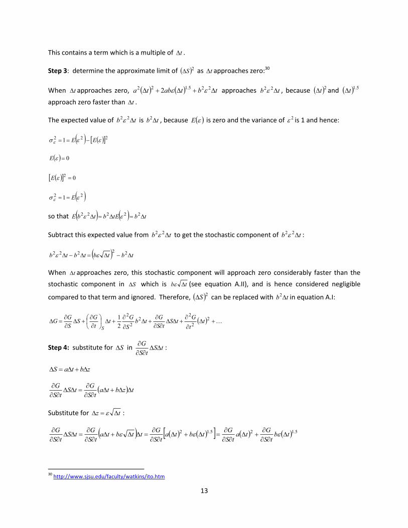
This contains a term which is a multiple of t .

Step 3: determine the approximate limit of 2S as t approaches zero:30

When t approaches zero, tbtabta 225.122 2 approaches tb 22 , because 2t and 5.1t

approach zero faster than t .

The expected value of tb 22 is tb 2 , because E is zero and the variance of 2 is 1 and hence:

22

2

222

1

0

0

1

E

E

E

EE

so that tbtEbtbE 22222

Subtract this expected value from tb 22 to get the stochastic component of tb 22 :

tbtbtbtb 22222

When t approaches zero, this stochastic component will approach zero considerably faster than the

stochastic component in S which is tb (see equation A.II), and is hence considered negligible

compared to that term and ignored. Therefore, 2S can be replaced with tb 2 in equation A.I:

2

2

22

2

2

2

1t

t

GtS

tS

Gtb

S

Gt

t

GS

S

GG

S

Step 4: substitute for S in tStS

G

:

zbtaS

tzbtatS

GtS

tS

G

Substitute for tz :

5.125.12tb

tS

Gta

tS

Gtbta

tS

Gttbta

tS

GtS

tS

G

30

http://www.sjsu.edu/faculty/watkins/ito.htm

14

As both summands are coefficients of t raised to higher powers than 1, they get both ignored (like

other such terms in the Taylor-series approximation), so that G simplifies to:

tbS

Gt

t

GS

S

GG

S

2

2

2

2

1

Step 5: substitute for delta S :

zbtaS

tbS

Gt

t

Gzbta

S

GG

S

2

2

2

2

1

Step 6: Rearranging:

zbS

Gtb

S

G

t

Ga

S

GG

S

2

2

2

2

1

Step 7: Taking limits ( t approaching zero) gives Ito’s Lemma:

bdzS

Gdtb

S

G

t

Ga

S

GdG

S

2

2

2

2

1

A process for stock prices:31

Sa

Sb

SdzSdtdS

or in discrete time:

A.III: tStSzStSS

Where return statistics (expected value and volatility) are given as p.a. figures and the unit of t is years.

This process is known as geometric Brownian motion. If the stock price follows this process, the stock’s

instantaneous return (discrete return in an (infinitesimal) small interval) is: dzdtS

dS .

31

See e.g. Hull, p. 308-309

15

Apply Ito’s Lemma to a function G of S and t:

A.IV.:

SdzS

GdtS

S

G

t

GS

S

GdG

S

22

2

2

2

1

Apply Ito’s lemma to LN(S):32

SLNG

0

1

1

2

2

2

2

1

t

G

SS

S

G

SSS

G

So in general, if S follows an Ito process, the process for G=LN(S) is:

bdzS

dtbS

aS

dG1

2

11 2

2

And more specifically, if S follows a geometric Brownian motion, so that SdzSdtdS , i.e. Sa and

Sb , the process for dG is:

dzdtdG

2

2

Hence:

dtdtNdG 2

2

,2

~

(i.e. dGe is “log-normally distributed” meaning that its logarithm is normally distributed).

and hence the following holds for the stock price after a short period of time:

dzdt

t eSeSS tdG

tdtt

2

2

i.e. with the instantaneous return dS/S being defined as above, dG is the return of the stock expressed

as rate of return with continuous compounding during time interval dt33.

32

Hull, p. 314-315

16

The expected value of a log-normally distributed variable w, whose logarithm is normally distributed

with mean m and standard deviation o is:34

2

2omewE

So that:

dtdG eSeESSE 00

An informal expression for the stock price after a period longer than dt:

With

dzdt

t eSeSS tdG

tdtt

2

2

, and as under the assumption of S following a geometric Brownian

motion, and are constant, one can derive an “informal”35 expression for the random variable St

after a longer period than dt, for example a period containing two (infinitesimal small) periods, i.e. two

periods with the length dt of each approaching zero – with the index t in St indicating the number of

such periods of length dt that will have passed:

212

2

2

2

22

2

12

2

22

2

12

2

22

2

2

12

2

1

0

00112

001

dzdzdtdt

dzdtdzdtdzdtdzdtdzdt

dzdt

eS

eSeeSeSeSS

eSeSS

dG

dG

Correspondingly, with T being the point in time after N such periods with a length dt that approaches

zero, the stock price at T is:

N

ttdzdtN

eSST12

2

0

Hence, the expected return 0SLNSLNE T with continuous compounding over the total period is:

33

For the definition of the rate of return with continuous compounding and its relationship to a discrete return under certainty see e.g. Hull, Options Futures & Other Derivatives, 9

th edition, page 81. For a discussion of the relationship between an

uncertain instantaneous return and the corresponding random return with continuous compounding and stock price, see Hull, section 15.3 (page 325). 34

See Hull technical note 2 to Options, Futures & Other Derivatives, (9th

ed). 35

a formal expression would use a stochastic integral over t.

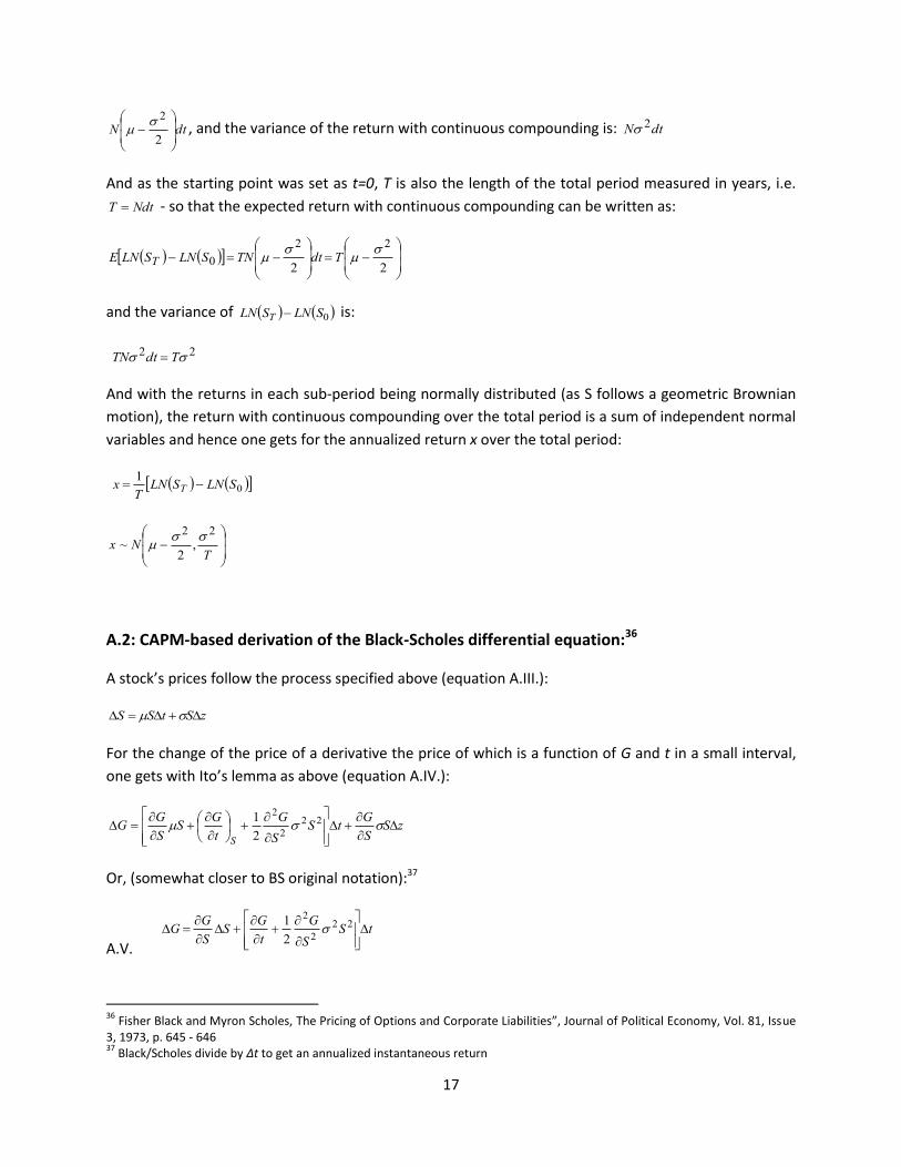
17

dtN

2

2 , and the variance of the return with continuous compounding is: dtN 2

And as the starting point was set as t=0, T is also the length of the total period measured in years, i.e.

NdtT - so that the expected return with continuous compounding can be written as:

22

22

0

TdtTNSLNSLNE T

and the variance of 0SLNSLN T is:

22 TdtTN

And with the returns in each sub-period being normally distributed (as S follows a geometric Brownian

motion), the return with continuous compounding over the total period is a sum of independent normal

variables and hence one gets for the annualized return x over the total period:

01

SLNSLNT

x T

TNx

22

,2

~

A.2: CAPM-based derivation of the Black-Scholes differential equation:36

A stock’s prices follow the process specified above (equation A.III.):

zStSS

For the change of the price of a derivative the price of which is a function of G and t in a small interval,

one gets with Ito’s lemma as above (equation A.IV.):

zSS

GtS

S

G

t

GS

S

GG

S

22

2

2

2

1

Or, (somewhat closer to BS original notation):37

A.V.

tSS

G

t

GS

S

GG

22

2

2

2

1

36

Fisher Black and Myron Scholes, The Pricing of Options and Corporate Liabilities”, Journal of Political Economy, Vol. 81, Issue 3, 1973, p. 645 - 646 37

Black/Scholes divide by Δt to get an annualized instantaneous return

18

Black/Scholes assume the CAPM holds for instantaneous returns.38

Derive the option’s beta: Write the instantaneous option return as function of the stock return S

S :

G

tS

S

G

t

G

G

S

S

S

S

G

G

G

22

2

2

2

1

Covariance of option return with market return:

MM r

S

tS

G

S

S

Gr

G

G,cov,cov

Hence, the option beta as a function of the underlying stock’s beta S is:

G

S

S

GS

If CAPM holds, the instantaneous expected return of the option must equal:

G

S

S

GtrrEtr

G

GE

G

S

S

GtrrEtr

G

GE

G

S

S

GtrrEtr

G

GE

S

SM

SM

Where Sr is the instantaneous return of the stock. The expected change in the option price is therefore:

A.VI.:

S

GtrStGrSE

S

GGE

The expected absolute change results also from taking the expected value of both sides of A.IV.:

A.VII.:

tSS

G

t

GSE

S

GGE

22

2

2

2

1

Setting A.VI. and A.VII. equal, subtracting SES

G

on both sides, dividing by t and simplifying gives the

Black-Scholes differential equation:39

2

222

2 S

GS

S

GrSrG

t

G

38

Black/Scholes page 646 and footnote 2 on page 639 39

Black/Scholes , equation 7, page 643