FEDERAL RESERVE BANK OF SAN FRANCISCO

WORKING PAPER SERIES

Pricing Deflation Risk with U.S. Treasury Yields

Jens H.E. Christensen Federal Reserve Bank of San Francisco

Jose A. Lopez

Federal Reserve Bank of San Francisco

Glenn D. Rudebusch Federal Reserve Bank of San Francisco

July 2014

The views in this paper are solely the responsibility of the authors and should not be interpreted as reflecting the views of the Federal Reserve Bank of San Francisco or the Board of Governors of the Federal Reserve System.

Working Paper 2012-07 http://www.frbsf.org/publications/economics/papers/2012/wp12-07bk.pdf

Pricing Deflation Risk

with U.S. Treasury Yields

Jens H. E. Christensen

Jose A. Lopez

and

Glenn D. Rudebusch

Federal Reserve Bank of San Francisco

Abstract

We use an arbitrage-free term structure model with spanned stochastic volatility to

determine the value of the deflation protection option embedded in Treasury inflation-

protected securities (TIPS). The model accurately prices the deflation protection option

prior to the financial crisis when its value was near zero; at the peak of the crisis in late 2008

when deflationary concerns spiked sharply; and in the post-crisis period. During 2009, the

average value of this option at the five-year maturity was 41 basis points on a par-yield

basis. The option value is shown to be closely linked to overall market uncertainty as

measured by the VIX, especially during and after the 2008 financial crisis.

JEL Classification: E43, E47, G12, G13.

Keywords: TIPS, deflation risk, term structure modeling.

We thank participants at the 2012 AFA meetings, FRB Chicago Day Ahead Conference, and the 15thAnnual Conference of the Swiss Society for Financial Market Research for helpful comments, especially ourdiscussants Kenneth Singleton, Andrea Ajello, and Rainer Baule. We also thank participants at the FDIC’s21st Derivatives Securities & Risk Management Conference, the Second Humboldt-Copenhagen Conference,and the Fourth Annual SoFiE Conference for helpful comments on previous drafts of the paper. Finally, wethank James Gillan and Justin Weidner for excellent research assistance. The views in this paper are solelythe responsibility of the authors and should not be interpreted as reflecting the views of the Federal ReserveBank of San Francisco or the Board of Governors of the Federal Reserve System.

This version: July 18, 2014.

1 Introduction

The U.S. Treasury first issued inflation-indexed bonds, which are now commonly known as

Treasury inflation-protected securities (TIPS), in 1997. TIPS provide inflation protection

since their coupons and principal payments are indexed to the headline Consumer Price

Index (CPI) produced by the Bureau of Labor Statistics.1 In addition, TIPS provide some

protection against price deflation since their principal payments are not permitted to decrease

below their original par value.

This deflation protection option has received limited attention in the literature, most

likely since it has not been of much value in the U.S. inflationary environment since 1997.

However, the sharp drops in price indexes during the financial crisis that started in the

fall of 2008 increased deflationary concerns markedly, thus providing further motivation for

examining the value of this protection. Two recent papers have used different arbitrage-free

term structure models to assess the values of these deflation protection options.

Grishchenko et al. (2013) use a Gaussian affine model whose two factors are nominal

Treasury rates and the inflation rate observed at the monthly frequency. They found that the

option value is close to zero for most months, except for the deflationary periods observed in

2003-2004 and in 2008-2009. They calculate the maximum observed option value in December

2008 to be roughly 45 basis points of TIPS par value. On a par-yield basis, assuming a

duration of four years for a five-year TIPS, this translates into a yield spread of approximately

10 basis points.

Christensen et al. (2012) use a “yields-only” approach based on a Gaussian affine model

developed by Christensen et al. (2010, henceforth CLR) to value these deflation protection

options. That model uses four factors to capture the joint dynamics of the nominal and real

Treasury yield curves. The first three factors can be characterized as the level, slope, and

curvature of the nominal yield curve, while the fourth factor can be characterized as the level

of the real yield curve. The authors find that the option value, measured as a par-yield spread

between two TIPS of similar remaining maturity but of differing vintages, reached a maximum

of almost 80 basis points in December 2008 for TIPS maturing in 2013. This option value

series is labeled the “CV model“ in Figure 1. While the model-implied option value is highly

correlated with the observed TIPS spread chosen as a proxy for the deflation protection option

value, the implied values are mainly lower than the observed values. The authors suggest that

this shortcoming could be addressed by incorporating stochastic volatility into the model in

the hope of better characterizing the lower tail of the model-implied distribution of inflation

outcomes.

1The actual indexation has a lag structure since the Bureau of Labor Statistics publishes price index valueswith a one-month lag; that is, the index for a given month is released in the middle of the subsequent month.The reference CPI is thus set to be a weighted average of the CPI for the second and third months prior tothe month of maturity. See Gurkaynak et al. (2010) for a detailed discussion as well as Campbell et al. (2009)for an overview of inflation-indexed bonds.

1

2008 2009 2010

050

100

150

200

250

300

2008 2009 2010

050

100

150

200

250

300

2008 2009 2010

050

100

150

200

250

300

Spr

ead

in b

asis

poi

nts

Lehman Brothers

Bankruptcy

Sept. 15, 2008

Yield spread of pair of 2013 TIPS Spread, CV model Spread, SV model

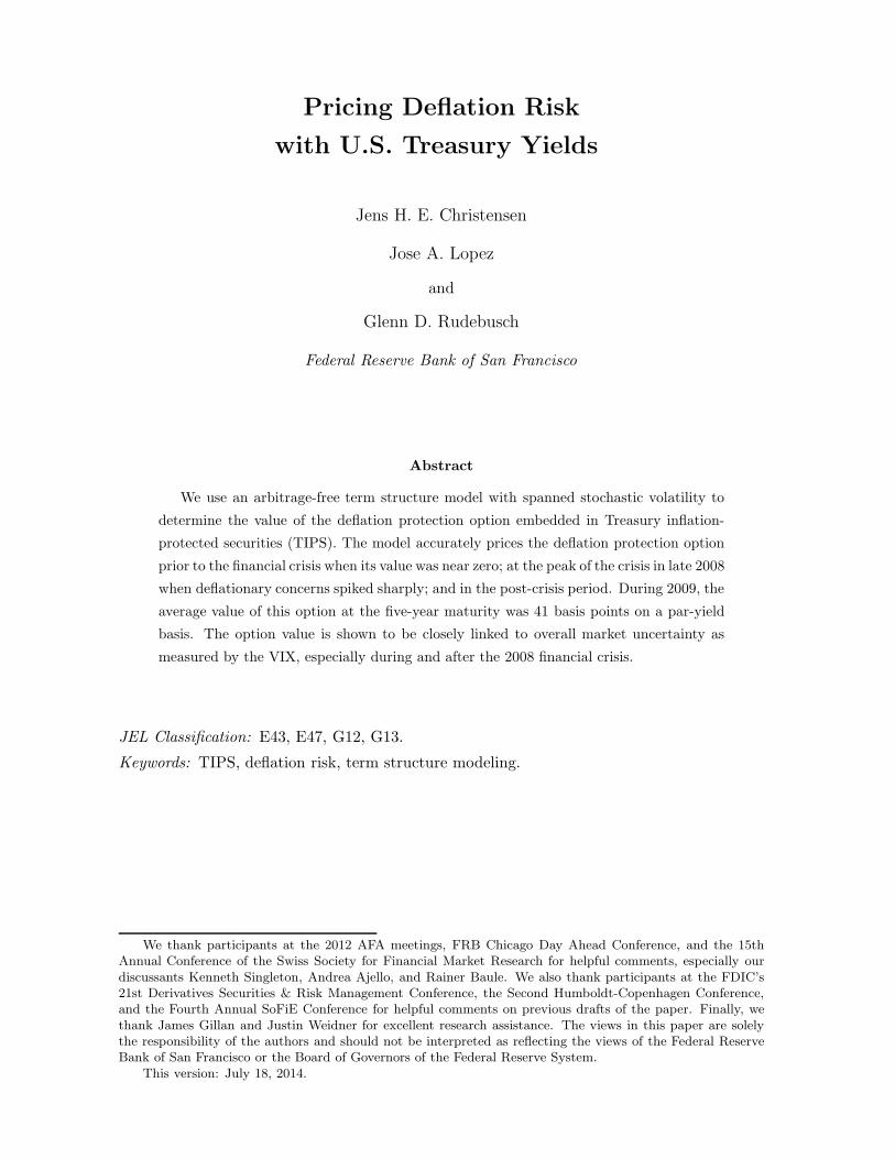
Figure 1: Yield Spread between a Pair of 2013 TIPS as a Proxy for the Value of

the Embedded Deflation Protection Option.

Illustration of the spread in the yield-to-maturity as reported by Bloomberg between the seasoned

ten-year TIPS that matures on July 15, 2013, and the newly issued five-year TIPS that matures on

April 15, 2013. Included are the model-implied five-year par-coupon yield spreads from the CV model

and the SV model introduced in this paper.

In this paper, we modify the latter model of nominal and real Treasury yields to incor-

porate spanned stochastic volatility.2 In particular, the volatility dynamics are specified to

be driven by the nominal and real level factors in the model. Using the same Treasury yield

data, the stochastic volatility (SV) model exhibits similar in-sample fit and out-of-sample

forecast performance relative to the constant volatility (CV) model. Specifically, the two

models’ transformations of their conditional mean specifications into such objects of interest

as five-year inflation expectations and inflation risk premiums exhibit similar dynamics. In

contrast, and more importantly for valuing the TIPS deflation protection option, the mod-

els exhibit important differences related to the transformations of their conditional volatility

dynamics into conditional distributions of headline CPI changes.

In particular, the one-year deflation probability forecasts generated by the SV model are

generally higher than those generated by the CV model. As might be expected, the differing

deflation probabilities lead to important differences in the model-implied values of the TIPS

deflation protection option. Figure 1 shows the yield spread between pairs of TIPS with

2Adrian and Wu (2010) also propose a model of nominal and real Treasury yields with spanned stochasticvolatility. In related research, Haubrich et al. (2012) and Fleckenstein et al. (2013) build models of inflationswap rates with stochastic volatility.

2

similar maturities, but differing degrees of accumulated inflation protection. This spread is

a proxy for the value of the embedded deflation protection option, as per Wright (2009). As

shown in the figure, the SV model generates a yield spread that more directly captures the

observed spread in the last few months of 2008 and into 2009. In fact, while both sets of

model-implied spreads have correlations of nearly 0.9 with the observed spread, the SV model

has a root mean squared error over 2009 of 9.5 basis points as compared to 28.7 basis points

for the CV model. In 2008 before the Lehman bankruptcy, the SV model-implied value of the

TIPS deflation protection option at the five-year maturity was 6.8 basis points. During the

height of the crisis period in late 2008, that value jumped to 89.1 basis points as deflationary

concerns rose markedly during the sharp economic contraction. For 2009 as a whole, the

average value of this option was 41 basis points on a par-yield basis, and that average value

declined to 19.5 for 2010. These results suggest that the SV model is well equipped to measure

and price deflation risk within the Treasury market, and thus it should be well placed to price

the inflation derivatives increasingly being traded in the United States.3

Finally, equipped with accurate estimates of the price of the embedded deflation protection

option, we study the market factors that influence its value. Specifically, we use regressions

to analyze the par-bond yield spread between a comparable seasoned and newly issued TIPS

discussed above, which we refer to as the deflation risk premium. The empirical challenge is

to assess what part of this deflation risk premium reflects outright deflation fears associated

with general economic uncertainty and what part is a reflection of market illiquidity and

limits to arbitrage.4 Our primary explanatory factor to account for the former is the VIX

options-implied volatility index, which represents near-term uncertainty about the general

stock market and is widely used as a gauge of investor risk aversion. We also include variables

that gauge market illiquidity, such as the economy-wide market illiquidity measure introduced

by Hu et al. (2013, henceforth HPW). Our empirical results suggest that general economic

uncertainty as reflected in the VIX is the main factor determining the deflation risk premium,

accounting for about 65% of its observed variation. However, liquidity effects also play a

role, particularly before and during the 2008-2009 financial crisis. Further research into this

important aspect of TIPS pricing and liquidity premia is needed.

The paper is structured as follows. Section 2 introduces the general theoretical framework

for inferring deflation dynamics from nominal and real Treasury yield curves and details our

proposed methodology for deriving the model-implied value of the deflation protection option.

Section 3 describes the term structure model with constant volatility as developed by CLR

as well as the specification of the SV model used for this study. Section 4 contains the data

description and the empirical results for the two models, while Section 5 analyzes the drivers

3See Christensen and Gillan (2012) for further discussion of U.S. inflation swaps and related liquidity issues.Kitsul and Wright (2013) examine inflation caps and floors to derive option-implied inflation probability densityfunctions.

4TIPS liquidity has been a concern historically, and not least at the peak of the financial crisis, see CLRand Fleckenstein et al. (2012) for detailed discussions.

3

of the deflation risk premium. Section 6 concludes and provides directions for future research.

The appendices contain additional technical details.

2 Pricing Deflation Risk with Treasuries and TIPS

In this section, we provide the theoretical foundation for the framework we use to price

deflation protection options.

2.1 Deriving Market-Implied Inflation Expectations and Risk Premiums

An arbitrage-free term structure model can be used to decompose the difference between

nominal and real Treasury yields, also known as the breakeven inflation (BEI) rate, into the

sum of inflation expectations and an inflation risk premium. We follow Merton (1974) and

assume a continuum of nominal and real zero-coupon Treasury bonds exist with no frictions

to their continuous trading. The economic implication of this assumption is that the markets

for inflation risk are complete in the limit. Define the nominal and real stochastic discount

factors, denoted MNt and MR

t , respectively. The no-arbitrage condition enforces a consistency

of pricing for any security over time. Specifically, the price of a nominal bond that pays one

dollar in τ years and the price of a real bond that pays one unit of the defined consumption

basket in τ years must satisfy the conditions that

PNt (τ) = EP

t

[MN

t+τ

MNt

]and PR

t (τ) = EPt

[MR

t+τ

MRt

],

where PNt (τ) and PR

t (τ) are the observed prices of the zero-coupon, nominal and real bonds

for maturity τ on day t and EPt [.] is the conditional expectations operator under the real-

world (or P -) probability measure. The no-arbitrage condition also requires a consistency

between the prices of real and nominal bonds such that the price of the consumption basket,

denoted as the overall price level Πt, is the ratio of the nominal and real stochastic discount

factors:

Πt =MR

t

MNt

.

We assume that the nominal and real stochastic discount factors have the standard dy-

namics given by

dMNt /MN

t = −rNt dt− Γ′tdW

Pt ,

dMRt /MR

t = −rRt dt− Γ′tdW

Pt ,

where rNt and rRt are the instantaneous, risk-free nominal and real rates of return, respectively,

and Γt is a vector of premiums on the risks represented by WPt . By Ito’s lemma, the dynamic

4

evolution of Πt is given by

dΠt = (rNt − rRt )Πtdt.

Thus, with the absence of arbitrage, the instantaneous growth rate of the price level is equal to

the difference between the instantaneous nominal and real risk-free rates.5 Correspondingly,

we can express the stochastic price level at time t+τ as

Πt+τ = Πte∫ t+τt

(rNs −rRs )ds.

The relationship between the yields and inflation expectations can be obtained by decom-

posing the price of the nominal bond as follows:

PNt (τ) = EP

t

[MN

t+τ

MNt

]= EP

t

[MR

t+τ/Πt+τ

MRt /Πt

]= EP

t

[MR

t+τ

MRt

Πt

Πt+τ

]

= EPt

[MR

t+τ

MRt

]× EP

t

[Πt

Πt+τ

]+ covPt

[MR

t+τ

MRt

,Πt

Πt+τ

]

= PRt (τ)× EP

t

[Πt

Πt+τ

]×(1 +

covPt

[MRt+τ

MRt

, ΠtΠt+τ

]

EPt

[MRt+τ

MRt

]× EP

t

[Πt

Πt+τ

]).

Converting this price into a yield-to-maturity using

yNt (τ) = −1

τlnPN

t (τ) and yRt (τ) = −1

τlnPR

t (τ), (1)

we obtain

yNt (τ) = yRt (τ) + πet (τ) + φt(τ), (2)

where the market-implied rate of inflation expected at time t for the period from t to t+ τ is

πet (τ) = −1

τlnEP

t

[Πt

Πt+τ

]= −1

τlnEP

t

[e−

∫ t+τt

(rNs −rRs )ds]

(3)

and the associated inflation risk premium for the same time period is

φt(τ) = −1

τln

(1 +

covPt

[MRt+τ

MRt

, ΠtΠt+τ

]

EPt

[MRt+τ

MRt

]× EP

t

[Πt

Πt+τ

]). (4)

Note that this inflation risk premium can be positive or negative, while the deflation risk

premium examined empirically in Section 5 is one-sided.

5We emphasize that the price level is a stochastic process as long as rNt and rRt are stochastic processes.

5

2.2 The Value of the Deflation Protection Embedded in TIPS

The primary focus of this paper is the value of the deflation protection embedded in TIPS

and how, during the financial crisis of 2008 and 2009, it affected the relative prices of pairs

of TIPS differentiated only by their accrued inflation compensation. Under standard infla-

tionary conditions, the value of the deflation protection should not play an important role in

TIPS pricing since the probability of having negative net accrued inflation compensation at

maturity is negligible; that is, the option should be well out-of-the-money. However, at the

peak of the financial crisis in the fall of 2008, neither the perceived nor the priced probability

of deflation were negligible as we show in Section 4. Under these circumstances, a wedge can

develop between the prices of seasoned TIPS with a significant amount of accrued inflation

compensation and recently issued on-the-run TIPS, which have no cumulated inflation com-

pensation. As suggested by Wright (2009), this wedge is a proxy for the value of the TIPS

deflation protection option.

To examine the ability of the proposed models to price these deflation protection options,

we use the models’ implied yield curves and deflation probabilities. We calculate the deflation

protection option values by comparing the prices of a newly issued TIPS without any accrued

inflation compensation and a seasoned TIPS with sufficient accrued inflation compensation

under the risk-neutral (or Q-) pricing measure. First, consider a hypothetical seasoned TIPS

with T years remaining to maturity that pays an annual coupon C semi-annually. Assume

this bond has accrued sufficient inflation compensation so it is nearly impossible to reach the

deflation floor before maturity. Under the risk-neutral pricing measure, the par-coupon bond

satisfying these criteria has a coupon rate determined by the equation

2T∑

i=1

C

2EQ

t

[e−

∫ tit rRs ds

]+ EQ

t

[e−

∫ Tt

rRs ds]= 1. (5)

The first term is the sum of the present value of the 2T coupon payments using the model’s

fitted real yield curve at day t. The second term is the discounted value of the principal

payment. The coupon payment of the seasoned bond that solves this equation is denoted as

CS .

Next, consider a new TIPS with no accrued inflation compensation with T years to ma-

turity. Since the coupon payments are not protected against deflation, the difference is in

accounting for the deflation protection on the principal payment. For this bond, the pricing

equation has an additional term; that is,

2T∑

i=1

C

2EQ

t

[e−

∫ tit rRs ds

]+ EQ

t

[ΠT

Πt

· e−∫ Tt

rNs ds1{ΠTΠt

>1}

]+ EQ

t

[1 · e−

∫ Tt

rNs ds1{ΠTΠt

≤1}

]= 1.

The first term is the same as before. The second term represents the present value of the

6

principal payment conditional on a positive net change in the price index over the bond’s

maturity; that is, ΠTΠt

> 1. Under this condition, full inflation indexation applies, and the

price change ΠTΠt

is placed within the expectations operator. The third term represents the

present value of the floored TIPS principal conditional on accumulated net deflation; that is,

when the price level change is below one, ΠTΠt

is replaced by a value of one to provide the

promised deflation protection.

SinceΠT

Πt

= e∫ Tt(rNs −rRs )ds,

the equation can be rewritten as

2T∑

i=1

C

2EQ

t [e−∫ tit rRs ds] + EQ

t

[e−

∫T

trRs ds

]+

[EQ

t

[e−

∫T

trNs ds1

{ΠTΠt

≤1}

]− EQ

t

[e−

∫T

trRs ds1

{ΠTΠt

≤1}

]]= 1,

where the last term on the left-hand side represents the net present value of the deflation

protection of the principal in the TIPS contract. The par-coupon yield of a new hypothetical

TIPS that solves this equation is denoted as C0. The difference between CS and C0 is a

measure of the advantage of being at the inflation adjustment floor for a newly issued TIPS

and thus of the value of the embedded deflation protection option.

3 Models of Nominal and Real Treasury Yield Curves

Given the theoretical framework introduced in the previous section, we briefly summarize

the affine term structure model of nominal and real Treasury yields with constant volatility

developed by CLR and then introduce the modified version with stochastic yield volatility.

Please note that even though the models are not formulated using the canonical form of affine

term structure models introduced by Dai and Singleton (2000), both models can be viewed

as restricted versions of their respective canonical model.6 Furthermore, it can be noted

that most of the restrictions imposed are motivated by a desire to generate a factor loading

structure in the zero-coupon bond yield functions that closely matches the popular Nelson

and Siegel (1987) model.

3.1 The Constant Volatility Model

The joint four-factor constant volatility (CV) model of nominal and real yields is a direct

extension of the three-factor, arbitrage-free Nelson-Siegel (AFNS) model developed by Chris-

tensen, Diebold and Rudebusch (2011, henceforth CDR) for nominal yields. In the CV model,

the state vector is denoted by Xt = (LNt , St, Ct, L

Rt ), where L

Nt is the level factor for nominal

yields, St is the common slope factor, Ct is the common curvature factor, and LRt is the level

6These restrictions can be derived explicitly, and the calculations are available upon request.

7

factor for real yields.7 The instantaneous nominal and real risk-free rates are defined as:

rNt = LNt + St, (6)

rRt = LRt + αRSt. (7)

Note that the differential scaling of the real rates to the common slope factor is captured

by the parameter αR. To preserve the Nelson-Siegel factor loading structure in the yield

functions, the risk-neutral (or Q-) dynamics of the state variables are given by the stochastic

differential equations:8

dLNt

dSt

dCt

dLRt

=

0 0 0 0

0 −λ λ 0

0 0 −λ 0

0 0 0 0

LNt

St

Ct

LRt

dt+Σ

dWLN ,Qt

dW S,Qt

dWC,Qt

dWLR,Qt

, (8)

where Σ is the constant covariance (or volatility) matrix.9 Based on this specification of

the Q-dynamics, nominal Treasury zero-coupon bond yields preserve the Nelson-Siegel factor

loading structure as

yNt (τ) = LNt +

(1− e−λτ

λτ

)St +

(1− e−λτ

λτ− e−λτ

)Ct −

AN (τ)

τ, (9)

where AN (τ)/τ is a maturity-dependent yield-adjustment term. Similarly, real TIPS zero-

coupon bond yields have a Nelson-Siegel factor loading structure expressed as

yRt (τ) = LRt + αR

(1− e−λτ

λτ

)St + αR

(1− e−λτ

λτ− e−λτ

)Ct −

AR(τ)

τ. (10)

Note that AR(τ)/τ is another maturity-dependent yield-adjustment term. These two equa-

tions, when combined in state-space form, constitute the measurement equation needed for

Kalman filter estimation.

To complete the model, we define the price of risk, which links the risk-neutral and real-

world yield dynamics, using the essentially affine risk premium specification introduced by

Duffee (2002). The real-world dynamics of the state variables are then expressed as

dXt = KP (θP −Xt)dt+ΣdWPt , (11)

7Chernov and Mueller (2012) provide evidence of a hidden factor in the nominal yield curve that is observablefrom real yields and inflation expectations. Our models accommodate this stylized fact via the LRt factor.

8As discussed in CDR, with unit roots in the two level factors, the model is not arbitrage-free with anunbounded horizon; therefore, as is often done in theoretical discussions, we impose an arbitrary maximumhorizon.

9As per CDR, Σ is a diagonal matrix, and θQ is set to zero without loss of generality.

8

which in its most general form can be written as10

dLNt

dSt

dCt

dLRt

=

κP11 κP12 κP13 κP14

κP21 κP22 κP23 κP24

κP31 κP32 κP33 κP34

κP41 κP42 κP43 κP44

θP1

θP2

θP3

θP4

−

LNt

St

Ct

LRt

dt+Σ

dWLN ,Pt

dW S,Pt

dWC,Pt

dWLR,Pt

. (12)

This equation is the transition equation used in the Kalman filter estimation.

3.2 The Stochastic Volatility Model

Financial time series, such as interest rates and bond yields, have been shown to have time-

varying volatility, which is a feature not often incorporated into arbitrage-free term structure

models; see Andersen and Benzoni (2010) for further discussion. To address this concern,

Christensen et al. (2014a) develop a general class of AFNS models that incorporate spanned

stochastic volatility. To distinguish between the various types of models, we use the notation

outlined in Dai and Singleton (2000) for classifying affine term structure models, such that

the CV model is within the A0(4) class of models that do not have volatility dynamics. As

detailed in Christensen et al. (2014a), there are several possible volatility specifications within

their three-factor framework, and clearly, the introduction of the fourth factor within the CLR

model generates an even larger set of possible specifications.

For this paper, we chose an A2(4) volatility specification that incorporates stochastic

volatility based on the nominal and real level factors. This choice was motivated by a desire

to focus on the longer maturity TIPS yields, since observable proxies for the value of the

TIPS deflation protection option are most available near the five-year maturity point.11 For

this stochastic volatility (SV) model, the state vector and instantaneous risk-free rates are

the same as before. To preserve the Nelson-Siegel factor loading structure and impose our

volatility specification, the Q-dynamics of the state variables are given by12

dLNt

dSt

dCt

dLRt

=

κQLN

0 0 0

0 λ −λ 0

0 0 λ 0

0 0 0 κQLR

θQLN

0

0

θQLR

−

LNt

St

Ct

LRt

dt (13)

10The model specification given by Equations (6), (7), (8), and (12) has 14 restrictions relative to its canonicalA0(4) model.

11Please note that the empirical results for the A1(4) specifications using just the nominal or real levelfactors are qualitatively similar, although quantitatively worse than the A2(4) specification. These results areavailable upon request.

12While the modeling framework allows for the two level factors to directly affect the volatility of thecommon slope and curvature factors, we fix the associated volatility sensitivity parameters to zero as perChristensen et al. (2014a), who report that these volatility sensitivity parameters are typically insignificantfor U.S. Treasury data. This choice leads to analytical bond pricing formulas that greatly facilitate modelestimation and analysis.

9

+

σ11 0 0 0

0 σ22 0 0

0 0 σ33 0

0 0 0 σ44

√LNt 0 0 0

0√1 0 0

0 0√1 0

0 0 0√

LRt

dWLN ,Qt

dW S,Qt

dWC,Qt

dWLR,Qt

.

The representation of the nominal zero-coupon bond yield function becomes

yNt (τ) = gN(κQLN

)LNt +

(1− e−λτ

λτ

)St +

(1− e−λτ

λτ− e−λτ

)Ct −

AN(τ ;κQ

LN

)

τ, (14)

where gN(κQLN

)is a modified loading on the nominal level factor.13 Note that the slope and

the curvature factor preserve their Nelson-Siegel factor loadings exactly, although the struc-

ture of the yield-adjustment term AN(τ ;κQ

LN

)/τ is different than before. Correspondingly,

the real zero-coupon bond yield function is now

yRt (τ) = gR(κQLR

)LRt + αR

(1− e−λτ

λτ

)St + αR

(1− e−λτ

λτ− e−λτ

)Ct −

AR(τ ;κQ

LR

)

τ, (15)

where gR(κQLR

)is a modified loading on the real level factor and AR

(τ ;κQ

LR

)/τ is a modified

yield-adjustment term.14

To link the risk-neutral and real-world dynamics of the state variables, we here use the

extended affine risk premium specification introduced by Cheridito et al. (2007), as per

Christensen et al. (2014a). The maximally flexible affine specification of the P -dynamics is

thus15

dLNt

dSt

dCt

dLRt

=

κP11 0 0 κP14

κP21 κP22 κP23 κP24

κP31 κP32 κP33 κP34

κP41 0 0 κP44

θP1

θP2

θP3

θP4

−

LNt

St

Ct

LRt

dt (16)

+

σ11 0 0 0

0 σ22 0 0

0 0 σ33 0

0 0 0 σ44

√LNt 0 0 0

0√1 0 0

0 0√1 0

0 0 0√

LRt

dWLN ,Pt

dW S,Pt

dWC,Pt

dWLR,Pt

.

To keep the model arbitrage-free, the two level factors must be prevented from hitting the

lower zero-boundary. This positivity requirement is ensured by imposing the Feller conditions

13Analytical formulas for gN(

κQLN

)

, gR(

κQLR

)

, AN(

τ ;κQLN

)

, and AR(

τ ;κQLR

)

are provided in Appendix A.14In our implementation, we fix κQ

LN= κQ

LR= 10−7 to get a close approximation to the uniform level factor

loading in the CV model.15The specification given by Equations (6), (7), (13), and (16) has 20 restrictions relative to its canonical

A2(4) model.

10

under both probability measures, which in this case are four; that is,

κP11θP1 + κP14θ

P4 >

1

2σ211,

10−7 · θQLN

>1

2σ211,

κP41θP1 + κP44θ

P4 >

1

2σ244,

and

10−7 · θQLR

>1

2σ244.

Furthermore, to have well-defined processes for LNt and LR

t , the sign of the effect that these

two factors have on each other must be positive, which requires the restrictions that

κP14 ≤ 0 and κP41 ≤ 0.

These conditions ensure that the two square-root processes will be non-negatively correlated.16

3.2.1 Deflation Probabilities within the SV Model

Christensen et al. (2012) use the CV model to generate deflation probabilities at various

horizons appropriate for macroeconomic and monetary policy purposes. Similarly, the SV

model can be used to calculate deflation probabilities, although additional steps are necessary.

The change in the price index implied by the model’s “yields-only” approach for the period

from t to t+ τ is given byΠt+τ

Πt

= e∫ t+τt

(rNs −rRs )ds.

To determine whether the change in the price index over a τ -period horizon may be below a

critical level q, we are interested in the probability of the states where

Πt+τ

Πt

≤ 1 + q,

or, equivalently,

Yt,τ =

∫ t+τ

t

(rNs − rRs )ds ≤ ln(1 + q).

Given that rNt = LNt + St and rRt = LR

t + αRSt, we are interested in the distributional

16Our empirical results show that the Feller condition pertaining to the real yield level factor LRt underthe Q-measure is systematically binding, while the other three Feller conditions are never binding. Thus, itis mainly the dynamics of LRt that are affected by the imposition of the Feller conditions, most notably σ44.For robustness, we analyzed the specification of the SV model without Feller conditions imposed, but found itto underperform along multiple dimensions relative to the reported SV model with Feller conditions imposed.Results for this alternative specification and analysis are available upon request.

11

properties of the process

Y0,t =

∫ t

0(rNs −rRs )ds =

∫ t

0(LN

s +Ss−LRs −αRSs)ds ⇒ dY0,t = (LN

t +(1−αR)St−LRt )dt.

This process is then introduced into the system of equations containing the P -dynamics of

the state variables Xt.

Due to the introduction of stochastic volatility into the two level factors, this system

of equations no longer has Gaussian state variables. As a consequence, we must use the

Fourier transform analysis described in full generality for affine models in Duffie, Pan, and

Singleton (2000), as opposed to the approach detailed in Christensen et al. (2012) for the CV

model. The intuition of this approach is to express expectations of contingent payments in a

tractable, mathematical form. By simplifying these expectations to indicator variables such

as 1(Yt,τ≤ln(1+q)), event probabilities are readily generated; see Appendix C for details.

3.3 Model Estimation

As noted above, the SV model is non-Gaussian, which prevents us from using some of the

recently proposed estimation techniques, such as Joslin et al (2011). Instead, the estimation

of both models relies on the Kalman filter as in CLR and Christensen et al. (2012); that is,

nominal and real zero-coupon yields are affine functions of the state variables such that

yt(τ) = −1

τB(τ)′Xt −

1

τA(τ) + εt(τ),

where εt(τ) are assumed to be i.i.d. Gaussian errors. The conditional mean for multi-

dimensional affine diffusion processes is given by

EP [XT |Xt] = (I − exp(−KP (T − t)))θP + exp(−KP (T − t))Xt, (17)

where exp(−KP (T−t)) is a matrix exponential. In general, the conditional covariance matrix

for affine diffusion processes is given by

V P [XT |Xt] =

∫ T

t

exp(−KP (T − s))ΣD(EP [Xs|Xt])D(EP [Xs|Xt])′Σ′ exp(−(KP )′(T − s))ds. (18)

Stationarity of the system under the P -measure is ensured if the real components of all

the eigenvalues of KP are positive, and this condition is imposed in all estimations. For this

reason, we can start the Kalman filter at the unconditional mean and covariance matrix.17

However, the introduction of stochastic volatility in the SV model implies that the factors

are no longer Gaussian since their variances are now dependent on the path of the state

17In the estimation, we calculate the conditional and unconditional covariance matrices using the analyticalsolutions provided in Fisher and Gilles (1996), which differs from the previous studies by CLR and Christensenet al. (2012) that relied upon numerical approximations.

12

variables. For tractability, we choose to approximate the true probability distribution of the

state variables using the first and second moments described above and use the Kalman filter

algorithm as if the state variables were Gaussian.18 The state equation is given by

Xt = (I − exp(−KP∆t))θP + exp(−KP∆t)Xt−1 + ηt, ηt ∼ N(0, Vt−1),

where ∆t is the time between observations and Vt−1 is the conditional covariance matrix given

in Equation (18).19 In the Kalman filter estimations, the error structure is given by

(ηt

εt

)∼ N

[(0

0

),

(Vt−1 0

0 H

)],

where H is assumed to be a diagonal matrix of the measurement error standard deviations,

σε(τi), that are specific to each yield maturity in the data set. Furthermore, the discrete

nature of the transition equation can cause the square-root processes to become negative

despite the fact that the parameter sets are forced to satisfy Feller conditions and other non-

negativity restrictions. Whenever this happens, we follow the literature and simply truncate

those processes at zero; see Duffee (1999) for an example.

4 Empirical Analysis

In this section, we first detail the data used for model estimation before describing the esti-

mation results with particular emphasis on the risk of deflation and its implications for the

value of the deflation protection options embedded in TIPS.

4.1 Data

In this paper, the nominal Treasury bond yields used are zero-coupon yields constructed as

in Gurkaynak et al. (2007).20 These yields are constructed using a discount function of the

Svensson (1995)-type to minimize the pricing error of a large pool of underlying off-the-run

Treasury bonds. As demonstrated by Gurkaynak et al. (2007), the model fits the underlying

pool of bond prices extremely well. By implication, the zero-coupon yields derived from this

approach constitute a very good approximation of the underlying Treasury zero-coupon yield

18A few notable examples of papers that follow this approach include Duffee (1999), Driessen (2005), andFeldhutter and Lando (2008). An unreported simulation analysis suggests that the added bias from using theKalman filter in estimating the SV model is modest relative to the finite-sample bias that even the CV modelis subject to.

19For estimation purposed over the first eight years of the sample with-

out TIPS yields, e−KP∆t, (1 − e−K

P∆t)θP , and the conditional covariance matrix∫ t+τ

te−K

P (t+τ−s)ΣD(EP [Xs|Xt])D(EP [Xs|Xt])′Σ′e−(KP )′(t+τ−s)ds are calculated using the upper (3 × 3)

part of KP and the upper (3× 1) part of θP .20The Board of Governors of the Federal Reserve updates the data on its website at

http://www.federalreserve.gov/pubs/feds/2006/index.html.

13

curve. From this dataset, we use eight Treasury zero-coupon bond yields with maturities of

3-months, 6-months, 1-year, 2-years, 3-years, 5-years, 7-years, and 10-years. We use weekly

Friday data and limit our sample to the period from January 6, 1995, to December 31, 2010,

which provides us with 835 weekly observations.21 Similarly, for the real Treasury yields, we

use the zero-coupon bond yields constructed with the same method used by Gurkaynak et

al. (2010).22 The data is available from January 1999, but due to weak liquidity in the first

years of TIPS trading, we follow CLR and limit our sample to the period after 2002. We

have weekly real Treasury yields from January 2, 2003, to December 31, 2010, a total of 418

observations. Since our focus is on the long-term real yields, we use the six yearly maturities

from five to ten years.

4.2 Estimation Results

To select the best fitting specifications of each model’s real-world dynamics, we use a general-

to-specific modeling strategy that restricts the least significant parameter in the estimation

to zero and then re-estimates the model. This strategy of eliminating the least significant

coefficients is carried out down to the most parsimonious specification, which has a diagonal

KP matrix. The final specification choice is based on the values of the Akaike and Bayes

information criteria as per CLR.23

For the CV model, the summary statistics of the model selection process are reported in

Table 1. Both information criteria are minimized by specification (9), which has a KP matrix

specified as

KPCV =

κP11 0 0 0

κP21 κP22 κP23 0

0 0 κP33 0

κP41 κP42 0 κP44

.

Table 2 contains the estimated parameters for this specification. All the off-diagonal elements

are highly significant and consistent with the empirical results reported in CLR.24 In terms

of dynamic properties, the nominal level factor is a persistent, slowly varying process not

affected by any of the other factors. The common curvature factor is also unaffected by the

other factors, but is less persistent and more volatile. The common slope factor is in between

these two extremes as it is less persistent than the nominal level factor and less volatile than

21We end the sample in 2010 to avoid having to address the complex problem of respecting the zero lowerbound for nominal yields, which appears to have been severe since August 2011 when the FOMC first providedexplicit forward guidance for future monetary policy. To support the view that this was less critical in 2009 and2010, we point to Swanson and Williams (2014), who provide evidence that medium- and long-term Treasuryyields responded to economic news during those two years in much the same way as in the prior decades.

22This dataset is also maintained by the Board of Governors of the Federal Reserve System athttp://www.federalreserve.gov/pubs/feds/2008/index.html.

23See Harvey (1989) for further details.24The primary difference with the specification favored by CLR is that the κP14 parameter is set to zero in

this case.

14

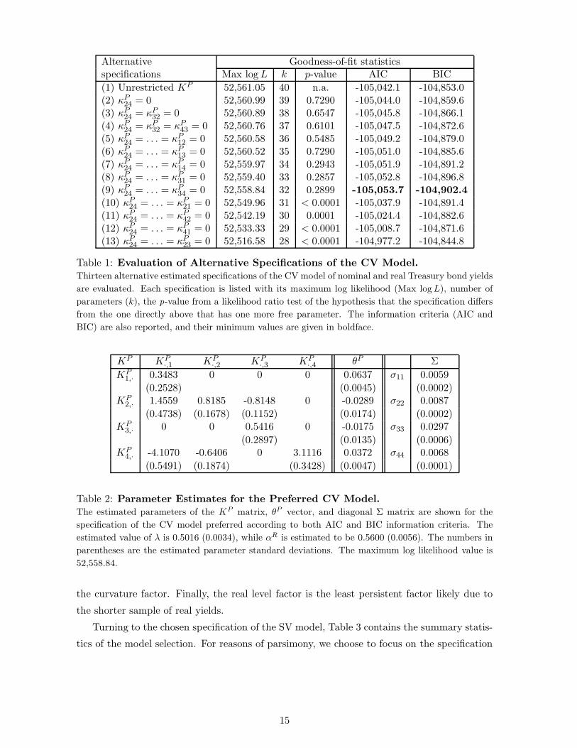
Alternative Goodness-of-fit statisticsspecifications Max logL k p-value AIC BIC

(1) Unrestricted KP 52,561.05 40 n.a. -105,042.1 -104,853.0(2) κP24 = 0 52,560.99 39 0.7290 -105,044.0 -104,859.6(3) κP24 = κP32 = 0 52,560.89 38 0.6547 -105,045.8 -104,866.1(4) κP24 = κP32 = κP43 = 0 52,560.76 37 0.6101 -105,047.5 -104,872.6(5) κP24 = . . . = κP12 = 0 52,560.58 36 0.5485 -105,049.2 -104,879.0(6) κP24 = . . . = κP13 = 0 52,560.52 35 0.7290 -105,051.0 -104,885.6(7) κP24 = . . . = κP14 = 0 52,559.97 34 0.2943 -105,051.9 -104,891.2(8) κP24 = . . . = κP31 = 0 52,559.40 33 0.2857 -105,052.8 -104,896.8(9) κP24 = . . . = κP34 = 0 52,558.84 32 0.2899 -105,053.7 -104,902.4

(10) κP24 = . . . = κP21 = 0 52,549.96 31 < 0.0001 -105,037.9 -104,891.4(11) κP24 = . . . = κP42 = 0 52,542.19 30 0.0001 -105,024.4 -104,882.6(12) κP24 = . . . = κP41 = 0 52,533.33 29 < 0.0001 -105,008.7 -104,871.6(13) κP24 = . . . = κP23 = 0 52,516.58 28 < 0.0001 -104,977.2 -104,844.8

Table 1: Evaluation of Alternative Specifications of the CV Model.

Thirteen alternative estimated specifications of the CV model of nominal and real Treasury bond yields

are evaluated. Each specification is listed with its maximum log likelihood (Max logL), number of

parameters (k), the p-value from a likelihood ratio test of the hypothesis that the specification differs

from the one directly above that has one more free parameter. The information criteria (AIC and

BIC) are also reported, and their minimum values are given in boldface.

KP KP·,1 KP

·,2 KP·,3 KP

·,4 θP Σ

KP1,· 0.3483 0 0 0 0.0637 σ11 0.0059

(0.2528) (0.0045) (0.0002)KP

2,· 1.4559 0.8185 -0.8148 0 -0.0289 σ22 0.0087

(0.4738) (0.1678) (0.1152) (0.0174) (0.0002)KP

3,· 0 0 0.5416 0 -0.0175 σ33 0.0297

(0.2897) (0.0135) (0.0006)KP

4,· -4.1070 -0.6406 0 3.1116 0.0372 σ44 0.0068

(0.5491) (0.1874) (0.3428) (0.0047) (0.0001)

Table 2: Parameter Estimates for the Preferred CV Model.

The estimated parameters of the KP matrix, θP vector, and diagonal Σ matrix are shown for the

specification of the CV model preferred according to both AIC and BIC information criteria. The

estimated value of λ is 0.5016 (0.0034), while αR is estimated to be 0.5600 (0.0056). The numbers in

parentheses are the estimated parameter standard deviations. The maximum log likelihood value is

52,558.84.

the curvature factor. Finally, the real level factor is the least persistent factor likely due to

the shorter sample of real yields.

Turning to the chosen specification of the SV model, Table 3 contains the summary statis-

tics of the model selection. For reasons of parsimony, we choose to focus on the specification

15

Alternative Goodness-of-fit statisticsspecifications Max logL k p-value AIC BIC

(1) Unrestricted KP 54,479.99 38 n.a. -108,884.0 -108,704.3(2) κP34 = 0 54,479.99 37 1.0000 -108,886.0 -108,711.1(3) κP34 = κP24 = 0 54,479.85 36 0.5967 -108,887.7 -108,717.5(4) κP34 = κP24 = κP31 = 0 54,479.26 35 0.2774 -108,888.5 -108,723.1(5) κP34 = . . . = κP32 = 0 54,479.12 34 0.5967 -108,890.2 -108,729.5(6) κP34 = . . . = κP21 = 0 54,477.19 33 0.0495 -108,888.4 -108,732.4(7) κP34 = . . . = κP41 = 0 54,473.33 32 0.0055 -108,882.7 -108,731.4(8) κP34 = . . . = κP14 = 0 54,470.80 31 0.0245 -108,879.6 -108,733.0

(9) κP31 = . . . = κP23 = 0 54,437.41 30 < 0.0001 -108,814.8 -108,673.0

Table 3: Evaluation of Alternative Specifications of the SV Model

Nine alternative estimated specifications of the SV model of nominal and real Treasury bond yields

are evaluated. Each specification is listed with its log likelihood (Max logL), number of parameters

(k), the p-value from a likelihood ratio test of the hypothesis that the specification differs from the

one directly above that has one more free parameter. The information criteria (AIC and BIC) are also

reported, and their minimum values are given in boldface.

preferred according to BIC with a mean-reversion matrix given by

KPSV =

κP11 0 0 0

0 κP22 κP23 0

0 0 κP33 0

0 0 0 κP44

.

Compared to the preferred specification of the CV model, κP21 and κP41 are jointly only bor-

derline significant, while κP42 is not admissible.

The estimated parameters for this preferred specification are reported in Table 4. The

most notable difference relative to the results for the CV model is that the nominal level factor

is less persistent, while the real level factor is more persistent. Furthermore, for obvious

reasons, σ11 and σ44 operate at different levels now due to the introduction of stochastic

volatility through the first and fourth factor. However, as we show below, these differences

do not lead to major differences in the models’ first moment dynamics.

Table 5 contains summary statistics for the fitted errors from both models. For the

nominal yields, the CV model fits the very short end of the nominal yield curve relatively

better than the longer maturities in the one- to ten-year maturity range. In contrast, the SV

model provides a better in-sample fit in the one- to ten-year maturity range, but less accurate

fit for short-maturity yields. For the real yields, though, the SV model provides a significant

overall improvement in model fit relative to the CV model, which is the main cause for the

large difference in likelihood values.

In the following, we analyze the performance of the two models in greater detail using real-

time analysis that adds one week of additional data to the estimation sample for each model

16

KP KP·,1 KP

·,2 KP·,3 KP

·,4 θP Σ

KP1,· 1.0431 0 0 0 0.0425 σ11 0.0633

(0.4193) (0.0045) (0.0006)KP

2,· 0 0.6711 -0.6248 0 -0.0118 σ22 0.0130

(0.1867) (0.1549) (0.0143) (0.0003)KP

3,· 0 0 0.6915 0 -0.0076 σ33 0.0303

(0.1966) (0.0119) (0.0007)KP

4,· 0 0 0 1.4203 0.0168 σ44 0.0597

(0.1914) (0.0017) (0.0007)

Table 4: Parameter Estimates for the Preferred SV Model.

The estimated parameters of the KP matrix, the θP vector, and the Σ matrix for the preferred

specification of the SV model according to BIC. The Q-related parameters are estimated at: λ = 0.6067

(0.0025), αR = 0.4397 (0.0068), θQLN

= 32,419 (31.67), and θQLR

= 17,846 (47.15). The numbers in

parentheses are the estimated standard deviations of the parameter estimates. The maximum log

likelihood value is 54,470.80.

Maturityin months

CV model SV model

Nom. yields Mean RMSE σε(τi) Mean RMSE σε(τi)

3 -0.54 9.53 9.51 0.75 19.23 19.226 0.00 0.00 0.00 -0.17 8.23 8.2412 1.79 5.80 5.79 0.00 0.00 0.0024 2.22 3.98 4.00 0.46 1.56 1.5636 0.00 0.13 0.55 0.00 0.00 0.0060 -2.67 3.73 3.83 -0.28 1.27 1.3884 0.08 3.37 3.66 0.24 0.59 1.14120 9.53 12.03 12.15 -1.15 4.41 4.59

TIPS yields Mean RMSE σε(τi) Mean RMSE σε(τi)

60 -3.98 20.27 20.20 -2.04 13.59 13.5972 -2.60 12.23 12.18 -0.51 5.87 5.8684 -1.31 5.64 5.61 0.00 0.00 0.0096 0.00 0.00 0.00 -0.38 4.72 4.72108 1.35 4.94 4.90 -1.52 8.74 8.74120 2.74 9.32 9.25 -3.32 12.35 12.35

Max logL 52,558.84 54,470.80

Table 5: Summary Statistics of the Fitted Errors.

The mean and root mean squared fitted errors (RMSE) for the preferred specification of the CV and

SV models are shown. All numbers are measured in basis points. The nominal yields cover the period

from January 6, 1995, to December 31, 2010, while the real TIPS yields cover the period from January

3, 2003, to December 31, 2010.

estimation; that is, each model is estimated using the sample covering the twelve-year period

from January 6, 1995, to January 5, 2007, and relevant model output is calculated; then,

one week of data is added to the sample and the models are re-estimated, and another set of

model output is constructed. This process is continued until the sample ends on December

17

2007 2008 2009 2010 2011

−2

−1

01

23

4

Rat

e in

per

cent

Lehman BrothersBankruptcy

Sept. 15, 2008

CV model SV model SPF five−year inflation forecast

Figure 2: Estimated Five-Year Inflation Expectations.

Illustration of the estimated inflation expectations at the five-year horizon according to the CV and

SV models. Included is the median five-year forecast of CPI inflation from the Survey of Professional

Forecasters.

31, 2010.

4.3 Inflation Expectations

A key purpose of our joint models of nominal and real yields is to decompose BEI rates

into inflation expectations and inflation risk premiums for further analysis. To conduct this

analysis, we generate real-time, out-of-sample forecasts based on the rolling model estimation

procedure described previously.

Figure 2 illustrates the models’ market-implied expected inflation at the five-year horizon

as well as the median of the five-year CPI inflation forecast from the Survey of Professional

Forecasters (SPF). The preferred CV and SV models produce sharp declines in expected

inflation shortly after the Lehman bankruptcy in September 2008, which is consistent with

realized inflation; that is, headline CPI did register negative year-over-year changes during

2009 for the first time since 1955. Since the beginning of 2009, the two models suggest that

medium-term inflation expectations have stabilized, but at a lower level than what prevailed

prior to the financial crisis. This downward shift is consistent with the downward trend in the

SPF survey measure, but notably larger. Furthermore, it appears consistent with the trend

in CPI realizations, which has shifted down.25

25From the beginning of 2006 until the end of June 2008, the average annual rate of headline CPI inflation

18

2007 2008 2009 2010 2011

−4

−2

02

46

8

2007 2008 2009 2010 2011

−4

−2

02

46

8

2007 2008 2009 2010 2011

−4

−2

02

46

8

2007 2008 2009 2010 2011

−4

−2

02

46

8

Rat

e in

per

cent

CV model SV model One−year inflation swap rate Blue Chip CPI inflation forecast Headline CPI inflation

Figure 3: One-Year CPI Inflation Forecasts.

Illustration of year-over-year headline CPI inflation realizations are shown with a solid grey line. The

one-year inflation forecasts from the CV and SV models are shown with a dashed and solid black line,

respectively. Included are also the monthly Blue Chip one-year headline CPI inflation forecast (dashed

grey line) and the one-year zero-coupon inflation swap rate downloaded from Bloomberg (dotted black

line).

In Figure 3, the one-year inflation forecasts from the two models are compared to the

subsequent headline CPI realizations as well as the corresponding survey forecasts provided

by Blue Chip and the one-year inflation swap rate. Please note that both models and surveys

are unable to capture the large variation in headline CPI inflation. To compare the various

forecasts, Table 6 reports the results of aligning the model-generated inflation forecasts with

the release dates of the Blue Chip survey and calculating the forecast errors for the 36 months

from January 2007 through December 2009. In terms of matching headline CPI inflation, the

two models are at least on par with, if not ahead of, the Blue Chip survey forecasts and the

one-year inflation swap rate as measured by RMSEs.

In addition to the conditional expectations for future inflation studied so far, we also

analyze the models’ ability to match the unconditional moments of the CPI inflation process.

To do so, we calculate the unconditional mean and standard deviation of the one- and two-

year expected inflation from the two models and compare them to the corresponding statistics

for headline CPI inflation realizations since January 2000. The results are reported in Table

7. Interestingly, the unconditional mean from the CV and SV models are below the mean of

was log(218.815/195.3)/2.5 = 4.5 percent, while the average annual rate from mid-2008 through 2010 was amodest log(219.179/218.815)/2.5 = 0.1 percent.

19

Model Mean RMSE

Random Walk -39.35 349.34

Inflation swap -38.86 224.45Blue Chip 42.12 300.47

CV model 23.77 215.78SV model 46.29 225.06

Table 6: Comparison of Real-Time CPI Inflation Forecasts.

Summary statistics for one-year forecast errors of headline CPI inflation in real time. The Blue Chip

forecasts are mapped to the tenth of each month January 2007 to December 2009, a total of 36 monthly

forecasts. The comparable model forecast is generated on the nearest available business day prior to

the Blue Chip release. A similar principle is used for the collection of the corresponding inflation swap

rate forecast. The subsequent CPI realizations are year-over-year changes starting at the end of the

survey month. As a consequence, the random walk forecasts equal the past year-over-year change in

the CPI series as of the end of the survey month.

Unconditional distribution of πet (τ)

Model τ = 1 year τ = 2 yearsMean Std. dev. Mean Std. dev.

Headline CPI inflation 2.45 1.38 2.47 0.86

CV model 1.35 0.71 1.35 0.64SV model 1.91 1.30 1.90 1.00

Table 7: Moments from the Unconditional Distribution of Expected Inflation.

The mean and standard deviation of the unconditional distribution of the one- and two-year expected

inflation from the CV and SV models are shown. The parameters in each case are those estimated

as of December 31, 2010. The mean and standard deviation of the unconditional distribution of

expected headline CPI inflation outcomes are approximated by the mean and standard deviation of

the monthly one- and two-year headline CPI inflation realizations over the period from January 2000

until December 2010, a total of 132 observations, measured at a continuously compounded rate. All

numbers are measured in percent.

observed CPI realizations. However, in terms of the volatility of the price inflation process,

the SV model is able to match the observed values very closely, while the CV model generates

a distribution for inflation outcomes that is too narrow. This result suggests that the SV

model captures price inflation dynamics reasonably well, in particular inflation uncertainty,

even though no price indexes are used in the model estimation.

4.4 Deflation Probability Forecasts

Another relevant comparison measure for these models is their implied probability forecasts

of net deflation one year ahead, as presented in Christensen et al. (2012) and in Figure 4. The

risk of deflation in 2007 and leading up to the failure of Lehman Brothers in September 2008

was basically zero under both models. In late 2008, the models assigned a high probability to

net deflation over the following twelve-month period, which is consistent with the observed

20

2007 2008 2009 2010 2011

0.0

0.2

0.4

0.6

0.8

1.0

Pro

babi

lity Lehman Brothers

Bankruptcy

Sept. 15, 2008

CV model SV model

Figure 4: Estimated One-Year Objective Deflation Probabilities.

Illustration of the estimated probability of negative net inflation over the following one-year period

according to the CV and SV models.

negative year-over-year change in headline CPI observed during these months. The SV model

probabilities are markedly higher than the CV model probabilities starting at the end of 2008

through year-end 2010. These higher and more persistent probabilities are partly a reflection

of slightly lower short-term expected inflation within the SV model during this period (see

Figure 3), but mainly they are due to the SV model’s higher conditional volatility estimates

that make tail outcomes more likely. Furthermore, in light of the fact that the economy did

experience negative headline CPI inflation during 2009, we consider the deflation probability

forecasts from the CV model to be low, while the forecasts from the SV model appear more

reasonable with estimates in the 30% to 50% range through most of 2009.

4.5 Deflation Protection Option Values

In this section, we use our rolling estimation results to analyze the models’ ability to price the

deflation protection option embedded in TIPS using the methodology described in Section

2.2. To highlight the difference between the CV and SV models in this regard, Figure 5 shows

the two model-implied values of the embedded TIPS deflation protection option measured as

the difference in value between a newly issued TIPS and an otherwise identical seasoned TIPS

converted into par-coupon yield spreads. The shown series are synthetic, constant five-year

par-yield spreads implied by both models. The figure also shows the actually observed yield

differences between seasoned and recently issued TIPS with maturities in 2013, 2014, and

21

2008 2009 2010 2011

050

100

150

200

250

300

2008 2010

050

100

150

200

250

300

2008 2010

050

100

150

200

250

300

Spr

ead

in b

asis

poi

nts

Lehman BrothersBankruptcy

Sept. 15, 2008

Yield spread of seasoned over new TIPS Spread, CV model Spread, SV model

Figure 5: Five-Year Par-Coupon Yield Spread Between Seasoned and Newly Issued

TIPS.

Illustration of the estimated five-year par-coupon yield spread between a seasoned and a newly issued

TIPS according to the CV and SV models. Included is also the spread in yield-to-maturity between

comparable pairs of seasoned and newly issued TIPS with approximately five years remaining to

maturity as reported by Bloomberg. This series is a proxy for the value of the embedded deflation

protection options. See footnote 24 for complete details on the specific nominal and real bond pairs

used to generate the series.

2015. At each point in time, we only show the yield spread for the TIPS pair containing

the most recently issued five-year TIPS, which we refer to as the on-the-run pair, and that

represents the closest observable proxy to the model-implied constant-maturity yield spread.26

As observed by Christensen et al. (2012), the CV model consistently undervalues the

deflation protection option even though it captures its time-variation well. The SV model

is much more successful at matching the observed value of the deflation option prior to the

crisis, at the peak of the crisis, as well as in the post-crisis period. Table 8 shows that the

SV model provides better estimates of the embedded TIPS deflation option over the sample

period of April 2008 through December 2010 both in terms of mean fitted error (i.e., -1.50

basis points for the SV model relative to +10.49 basis points for the CV model) and root-mean

squared error (i.e., 19.28 versus 25.09 basis points). Looking more carefully at subperiods,

both models performed similarly prior to the Lehman bankruptcy in September 2008, but for

26Specifically, from April 23, 2008, to April 22, 2009, we use the five-year TIPS with maturity in April 2013and the ten-year TIPS with maturity in July 2013. From April 23, 2009, to April 23, 2010, we use the five-yearTIPS with maturity in April 2014 and the ten-year TIPS with maturity in July 2014. Since April 26, 2010,we use the five-year TIPS with maturity in April 2015 and the ten-year TIPS with maturity in July 2015.

22

2008 2009 2010 2011

−1

01

23

4

Rat

e in

per

cent

Lehman BrothersBankruptcy

Sept. 15, 2008

Yield of seasoned TIPS, Bloomberg GSW implied yield, CV model GSW implied yield, SV model

(a) Seasoned TIPS yield.

2008 2009 2010 2011

−1

01

23

4

Rat

e in

per

cent

Lehman BrothersBankruptcy

Sept. 15, 2008

Yield of new TIPS, Bloomberg GSW implied yield, CV model GSW implied yield, SV model

(b) New TIPS yield.

Figure 6: Comparison of Model-Implied TIPS Yields to Bloomberg Data.

Comparison of the model-implied yields based on GSW data to the yield-to-maturity of the seasoned

and newly issued TIPS as reported by Bloomberg.

the remainder of 2008, the SV model’s RMSE was lower at 50.6 basis points as compared to

the CV model’s value of 62.4 basis points. The SV model again outperformed the CV model

over the course of 2009 with an RMSE of 33.4 basis points relative to 40.5 basis points, and in

2010, the corresponding RMSE values were similar at 8.4 versus 7.1 basis points. The ability

of the SV model to handle the greater volatility observed during the financial crisis, while

performing as well as the CV model before and after the crisis period, is strong evidence in

favor of using this model for term structure modeling, especially for interest-rate derivatives

pricing and capturing the data’s second-moment dynamics.

To further illustrate the relative performance of these two models, we examine the fitted

values of the model-implied equivalents of the yield-to-maturity for each of the TIPS in the on-

the-run pair separately.27 For this exercise, we match the timing of the outstanding coupons

and principal for each bond exactly, although we neglect the lag in the inflation indexation

since such adjustments are typically small for medium-term bonds. Specifically, we generate

the net present value of the remaining bond payments using Equation (5) and the fitted

real yield curve to convert the bond price into yield-to-maturity. In addition, we add the

model-implied value of the deflation protection option before converting the bond price into

yield-to-maturity. We explicitly control for the accrued inflation compensation in the option

valuation; that is, the option will only be in the money provided that

ΠT

Πt

≤ 1

Πt/Π0,

27We are grateful to Kenneth Singleton for suggesting this exercise.

23

CV model SV modelTIPS yield

Mean RMSE Mean RMSE

(a) Seasoned 1.88 38.68 15.76 39.41(b) Newly issued -8.61 23.75 17.26 32.32

Yield spread (a-b) 10.49 25.09 -1.50 19.28

Five-year GSW yield 9.29 28.48 4.67 18.61

Table 8: Summary Statistics of Pricing Errors for Bloomberg Data.

The table reports the mean and the root mean squared pricing error of the yield-to-maturity for the

seasoned and newly issued TIPS in the pair of TIPS that contains the on-the-run five-year TIPS as

reported by Bloomberg. For comparison the last row reports the comparable in-sample mean and root

mean squared fitted error of the five-year TIPS yield in the Gurkaynak et al. (2010) data based on the

full sample estimation of each model. All numbers are measured in basis points. The data is weekly

covering the period from April 25, 2008 to December 31, 2010, a total of 141 observations.

where Πt/Π0 is the index ratio as of time t. Thus, the deflation experienced over the remaining

life of the bond, ΠT /Πt, has to negate the accumulated inflation experienced since the bond’s

issuance.

As shown in Figure 6, both models fit the bond-specific yield data relatively well outside

of the peak of the financial crisis in the fall of 2008 and the early part of 2009 when TIPS

liquidity was a concern. Table 8 shows that the SV model does not perform as well in pricing

the individual bonds as it does in capturing the spread and thus the embedded option values.

For the sample period, the SV model has larger mean errors for both the seasoned and newly-

issued TIPS. In terms of RMSE, its value for the seasoned bonds is on par with that of the CV

model, but it is much higher for the newly-issued bonds. As observed in Table 5 regarding the

models’ comparative in-sample fit for the nominal and real yield curves, the relative advantage

of the SV model is not obvious when examining the data’s first moment dynamics, whether

for the real yield curve or for individual bond yields. However, the model’s ability to price the

option values implicit in the spread between the on-the-run bond pairs reflects its advantage

in better capturing the data’s second moment dynamics. Thus, the introduction of stochastic

volatility into term structure models is an important extension for modeling interest rate risk

and derivatives pricing.

5 Analysis of the Deflation Risk Premium

In this section, we use regression analysis to identify the determinants of the deflation risk

premium defined as the par-bond yield spread between a seasoned and a comparable newly

issued TIPS as described in the previous section.28 Up front, we acknowledge that TIPS mar-

28This analysis and the choice of variables are heavily inspired by Christensen and Gillan (2014), who assessthe impact on frictions in the TIPS and inflation swap markets from the TIPS purchases included in theFederal Reserve’s second program of large-scale asset purchases, frequently referred to a QE2, that operatedfrom November 2010 through June 2011.

24

ket functioning, along with the functioning of so many other financial markets, was impaired

at the peak of the financial crisis, and our models do not readily account for such liquidity

effects. As a consequence, we attempt to assess how much of the variation in the deflation

risk premium during our sample period reflects outright deflation fears caused by economic

uncertainty, and how much could be associated with market illiquidity and limits to arbitrage.

5.1 Econometric Challenge

The correlation between states of the world with near-zero interest rates and states of the

world with deflation is intuitively high.29 Unfortunately, the near-zero interest rates in the

U.S. came about as a policy response to the freezing of financial markets. Thus, in the

data, poor market functioning coincides with low interest rates. Worse still, in the post-crisis

period when financial conditions started to normalize, the reverse pattern was observed; that

is, improvement in market functioning goes hand in hand with reduced risk of deflation. Thus,

in our regressions, the deflation protection premium, which is our dependent variable, will tend

to decline at the same time as measures of market functioning improve without the two having

a causal relationship. In short, the results could likely be interpreted as indicating that the

yield wedge between seasoned and newly issued TIPS was caused by limits to arbitrage, rather

than reflecting true expectations for deflation. This is the ultimate econometric challenge.

5.2 Dependent Variables

We define the deflation risk premium to be the synthetic par-coupon bond yield spread be-

tween a seasoned TIPS whose deflation protection option value can be assumed to be zero and

a newly issued TIPS where the option is at-the-money. To be consistent with the previous

analysis, we limit our focus to the five-year deflation risk premium series. These estimated

series from the two models are shown in Figure 7 and represent the dependent variables in

our regressions.

5.3 Explanatory Variables

In this section, we provide a brief description of the explanatory variables included in our

analysis. While the other factors to be considered are supposed to capture limits to arbitrage

or pricing frictions, our first and leading candidate is a measure of priced economic uncertainty,

namely the VIX options-implied volatility index. It represents near-term uncertainty about

the general stock market as reflected in one-month options on the S&P 500 stock price index

and is widely used as a gauge of investor fear and risk aversion. When the price of uncertainty

29To see this, invoke the Fisher equation that states that the nominal interest rate equals the real interestrate plus the rate of inflation. If, in addition, deflationary states are low-growth states with low real rates, thehigh correlation between low nominal interest rates and deflation is reinforced.

25

2003 2004 2005 2006 2007 2008 2009 2010 2011

050

100

150

200

Rat

e in

bas

is p

oint

s Lehman BrothersBankruptcy

Sept. 15, 2008

CV model SV model

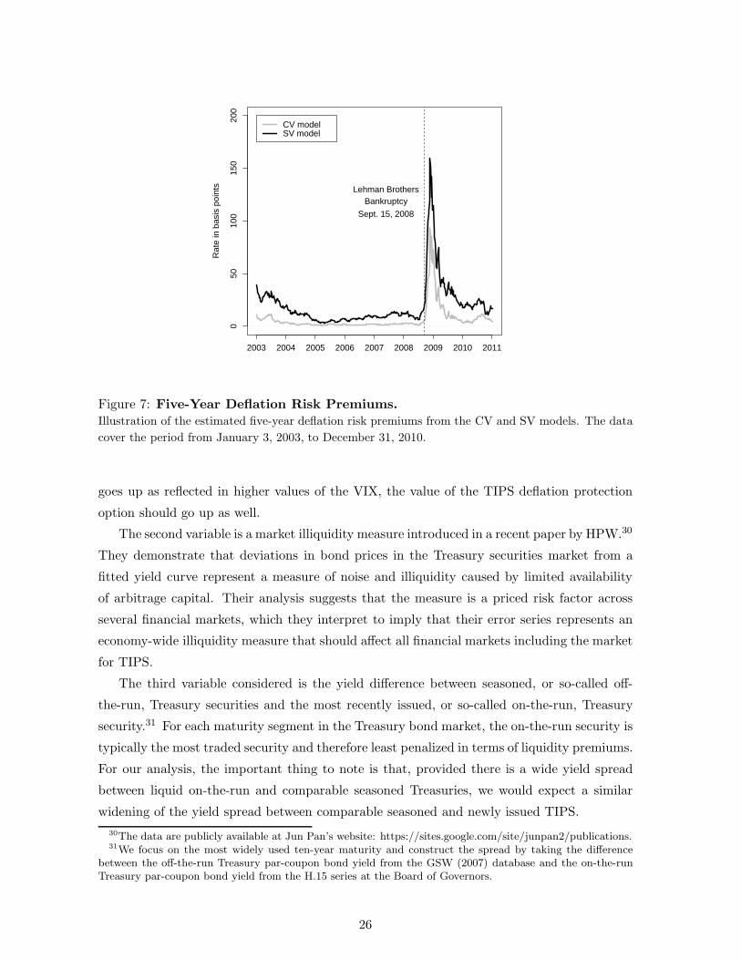
Figure 7: Five-Year Deflation Risk Premiums.

Illustration of the estimated five-year deflation risk premiums from the CV and SV models. The data

cover the period from January 3, 2003, to December 31, 2010.

goes up as reflected in higher values of the VIX, the value of the TIPS deflation protection

option should go up as well.

The second variable is a market illiquidity measure introduced in a recent paper by HPW.30

They demonstrate that deviations in bond prices in the Treasury securities market from a

fitted yield curve represent a measure of noise and illiquidity caused by limited availability

of arbitrage capital. Their analysis suggests that the measure is a priced risk factor across

several financial markets, which they interpret to imply that their error series represents an

economy-wide illiquidity measure that should affect all financial markets including the market

for TIPS.

The third variable considered is the yield difference between seasoned, or so-called off-

the-run, Treasury securities and the most recently issued, or so-called on-the-run, Treasury

security.31 For each maturity segment in the Treasury bond market, the on-the-run security is

typically the most traded security and therefore least penalized in terms of liquidity premiums.

For our analysis, the important thing to note is that, provided there is a wide yield spread

between liquid on-the-run and comparable seasoned Treasuries, we would expect a similar

widening of the yield spread between comparable seasoned and newly issued TIPS.

30The data are publicly available at Jun Pan’s website: https://sites.google.com/site/junpan2/publications.31We focus on the most widely used ten-year maturity and construct the spread by taking the difference

between the off-the-run Treasury par-coupon bond yield from the GSW (2007) database and the on-the-runTreasury par-coupon bond yield from the H.15 series at the Board of Governors.

26

Our fourth explanatory variable is the excess yield of AAA-rated U.S. industrial corporate

bonds over comparable Treasury yields.32 We note that in choosing the maturity we face a

trade off. On one side, we would ideally like to match the maturity of the deflation risk

premium measure. However, the credit risk of even AAA-rated industrial bonds cannot be

deemed negligible at a five-year horizon. On the other hand, if we focus on very short-term

debt where credit risk is entirely negligible, we are far from the desired maturity range. We

believe using the two-year credit spread strikes a reasonable balance. As the credit risk

component of such highly rated shorter-term bond yields is minimal, the yield spread largely

reflect the premium bond investors require for being exposed to the lower trading volume

and larger bid-ask spreads in the corporate bond market vis-a-vis the liquid Treasury bond

market. Again, if such illiquidity premiums of high-quality corporate bonds are large, we

could expect wider yield spreads between comparable seasoned and newly issued TIPS.

The fifth and final variable included is the weekly average of the daily trading volume

in the secondary market for TIPS as reported by the Federal Reserve Bank of New York.33

We use the 8-week moving average to smooth out short-term volatility. This measure should

have a negative effect on the deflation risk premium provided it reflects limits to arbitrage as

increases in TIPS trading volume should, in most cases, reduce mispricing.

5.4 Regression Results

Table 9 reports the results of regressing the five-year deflation risk premium measure from

the CV (top panel) and SV (bottom panel) models on the explanatory variables described in

the previous section.34

First, the regressions with the deflation risk premium measure from the SV model always

produce higher adjusted R2s than the regressions based on the deflation risk premium implied

by the CV model. Second, based on the measure from the SV model, the adjusted R2 easily

exceeds 80%. Thus, in general, we feel that our five explanatory variables are successful in

capturing the variation in the deflation risk premium. Third, and most importantly, the VIX

is always a highly significant explanatory variable with an estimated coefficient of the right

sign and of economically meaningful size. Thus, one robust finding is that financial market

uncertainty as measured by the VIX is a key determinant of the deflation risk premium as

represented by the at-the-money deflation protection option values implied by the CV and

SV models. Furthermore, and not surprisingly, the measure of financial market illiquidity

introduced by HPW also consistently has a high explanatory power with a positive sign for

its estimated coefficient. This suggests that at least part of the variation in our deflation risk

premium measure reflects financial market illiquidity. In addition, the other three measures of

market liquidity and market functioning, the off-the-run yield spread, the AAA credit spread,

32The data are from Bloomberg; See Christensen et al. (2014b) for details.33The data are available at: http://www.newyorkfed.org/markets/statrel.html.34The results reported in Table 9 are robust to using other maturities and sample periods.

27

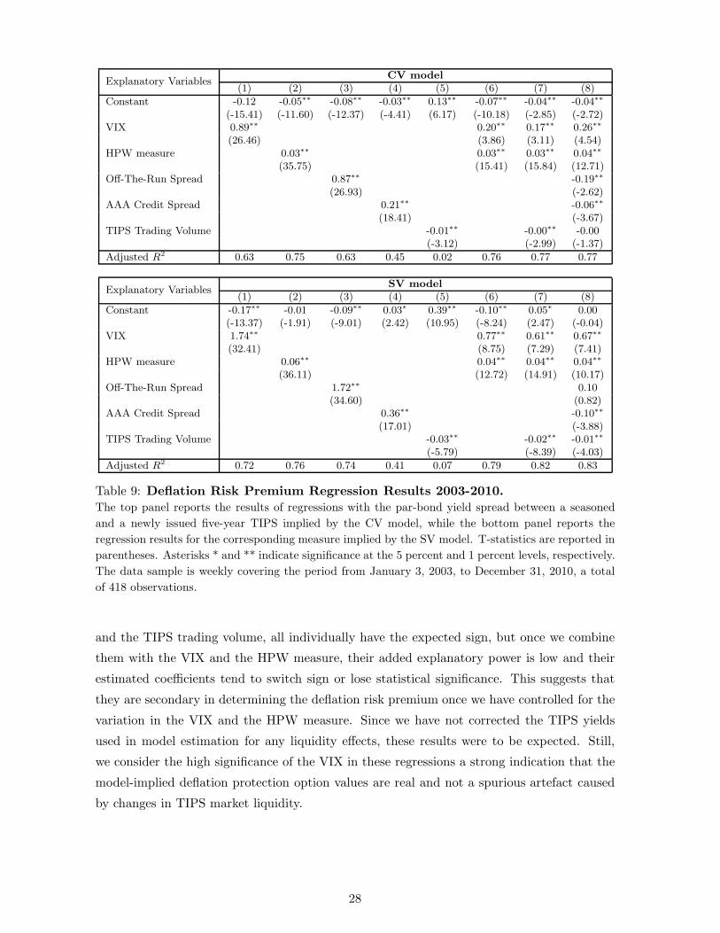
CV modelExplanatory Variables

(1) (2) (3) (4) (5) (6) (7) (8)

Constant -0.12 -0.05∗∗ -0.08∗∗ -0.03∗∗ 0.13∗∗ -0.07∗∗ -0.04∗∗ -0.04∗∗

(-15.41) (-11.60) (-12.37) (-4.41) (6.17) (-10.18) (-2.85) (-2.72)VIX 0.89∗∗ 0.20∗∗ 0.17∗∗ 0.26∗∗

(26.46) (3.86) (3.11) (4.54)HPW measure 0.03∗∗ 0.03∗∗ 0.03∗∗ 0.04∗∗

(35.75) (15.41) (15.84) (12.71)Off-The-Run Spread 0.87∗∗ -0.19∗∗

(26.93) (-2.62)AAA Credit Spread 0.21∗∗ -0.06∗∗

(18.41) (-3.67)TIPS Trading Volume -0.01∗∗ -0.00∗∗ -0.00

(-3.12) (-2.99) (-1.37)

Adjusted R2 0.63 0.75 0.63 0.45 0.02 0.76 0.77 0.77

SV modelExplanatory Variables

(1) (2) (3) (4) (5) (6) (7) (8)

Constant -0.17∗∗ -0.01 -0.09∗∗ 0.03∗ 0.39∗∗ -0.10∗∗ 0.05∗ 0.00(-13.37) (-1.91) (-9.01) (2.42) (10.95) (-8.24) (2.47) (-0.04)

VIX 1.74∗∗ 0.77∗∗ 0.61∗∗ 0.67∗∗

(32.41) (8.75) (7.29) (7.41)HPW measure 0.06∗∗ 0.04∗∗ 0.04∗∗ 0.04∗∗

(36.11) (12.72) (14.91) (10.17)Off-The-Run Spread 1.72∗∗ 0.10

(34.60) (0.82)AAA Credit Spread 0.36∗∗ -0.10∗∗

(17.01) (-3.88)TIPS Trading Volume -0.03∗∗ -0.02∗∗ -0.01∗∗

(-5.79) (-8.39) (-4.03)

Adjusted R2 0.72 0.76 0.74 0.41 0.07 0.79 0.82 0.83

Table 9: Deflation Risk Premium Regression Results 2003-2010.

The top panel reports the results of regressions with the par-bond yield spread between a seasoned

and a newly issued five-year TIPS implied by the CV model, while the bottom panel reports the

regression results for the corresponding measure implied by the SV model. T-statistics are reported in

parentheses. Asterisks * and ** indicate significance at the 5 percent and 1 percent levels, respectively.

The data sample is weekly covering the period from January 3, 2003, to December 31, 2010, a total

of 418 observations.

and the TIPS trading volume, all individually have the expected sign, but once we combine

them with the VIX and the HPW measure, their added explanatory power is low and their

estimated coefficients tend to switch sign or lose statistical significance. This suggests that

they are secondary in determining the deflation risk premium once we have controlled for the

variation in the VIX and the HPW measure. Since we have not corrected the TIPS yields

used in model estimation for any liquidity effects, these results were to be expected. Still,

we consider the high significance of the VIX in these regressions a strong indication that the

model-implied deflation protection option values are real and not a spurious artefact caused

by changes in TIPS market liquidity.

28

6 Conclusion

In this paper, we examine the deflation protection option embedded in TIPS over the period

from 2003 to 2010, including the depths of the financial crisis in late 2008 and early 2009.

To do so, we modify the joint model of nominal and real bond yields introduced in CLR

by replacing its constant volatility (CV) assumption with stochastic volatility (SV) driven

by the model’s nominal and real level factors. Our preferred specification of the SV model

delivers reasonable decompositions of breakeven inflation (i.e., the spread between nominal

and real Treasury yields) into expected inflation and inflation risk premiums, showing that

this model captures the data’s first moment dynamics as well as the CV model. However,

the SV model is shown to be better able to price the value of deflation protection embedded

in TIPS and proxied for here by the difference between similar TIPS with differing degrees

of accumulated inflation protection. This result highlights that the SV model is better able

to capture the volatility dynamics observed in the data and critical to derivatives pricing.

Based on this evidence, the proposed SV model should be useful for judging bond investors’

views on the tail risk of deflation as well as their inflation expectations. The SV model is

an obvious candidate for pricing derivative products in the inflation swap market, a topic we

leave for future research.

In analyzing the deflation risk premium defined as the par-bond yield spread between a

seasoned and a comparable newly issued TIPS, our results suggest that a significant part of

the variation in the deflation risk premium is associated with general economic uncertainty.

Still, a notable part of the variation is associated with measures of market illiquidity. Thus,

correcting TIPS yields for liquidity effects would be desirable (see Pflueger and Viceira 2013

and D’Amico et al. 2014 for examples), but this is another topic that we leave for future

research.

Finally, we end our sample in 2010 to avoid addressing the problem of the zero lower bound

of nominal yields. However, going forward, this will be a critical issue to address as short-term

U.S. Treasury yields have been near the zero lower bound since mid-2011. Christensen and

Rudebusch (2014) introduce a tractable shadow-rate AFNS model class, which respects the

zero lower bound for nominal bond yields and could be explored further. Again, we leave this

important endeavor for future research.

29

Appendices

A). Bond Price Formulas

In the SV model, nominal zero-coupon bond prices are given by

PN(t, T ) = EQt[

exp(

−∫ T

t

rNu du)]

= exp(

BN1 (t, T )LNt +BN2 (t, T )St+BN3 (t, T )Ct+B

N4 (t, T )LRt +AN(t, T )

)

,

where BN1 (t, T ), BN2 (t, T ), BN3 (t, T ), and BN4 (t, T ) are the unique solutions to the following system of ODEs

dBN1 (t,T )

dt

dBN2 (t,T )

dt

dBN3 (t,T )

dt

dBN4 (t,T )

dt

=

1

1

0

0

+

κQLN

0 0 0

0 λ 0 0

0 −λ λ 0

0 0 0 κQLR

BN1 (t, T )

BN2 (t, T )

BN3 (t, T )

BN4 (t, T )

−1

2

4∑

j=1

σ11 0 0 0

0 σ22 0 0

0 0 σ33 0

0 0 0 σ44

(BN1 )2 BN1 BN2 BN1 B

N3 BN1 B

N4

BN1 BN2 (BN2 )2 BN2 B

N3 BN2 B

N4

BN1 BN3 BN2 B

N3 (BN3 )2 BN3 B

N4

BN1 BN4 BN2 B

N4 BN3 B

N4 (BN4 )2

σ11 0 0 0

0 σ22 0 0

0 0 σ33 0

0 0 0 σ44

j,j

(δj)′,

and γ and δ are given by

γ =

0

1

1

0

and δ =

1 0 0 0

0 0 0 0

0 0 0 0

0 0 0 1

.

This structure implies that the factor loadings in the nominal zero-coupon bond price function are given

by the unique solution to the following set of ODEs

dBN1 (t, T )

dt= 1 + κQ

LNBN1 (t, T )− 1

2σ211B

N1 (t, T )2, BN1 (T, T ) = B

N

1 ,

dBN2 (t, T )

dt= 1 + λBN2 (t, T ), BN2 (T, T ) = B

N

2 ,

dBN3 (t, T )

dt= −λBN2 (t, T ) + λBN3 (t, T ), BN3 (T, T ) = B

N

3 ,

dBN4 (t, T )

dt= κQ

LRBN4 (t, T )− 1

2σ244B

N4 (t, T )2, BN4 (T, T ) = B

N

4 .

These four ODEs have the following unique solution35

BN1 (t, T ) =−2[eφ

N (T−t) − 1] +BN

1 eφN (T−t)(φN − κQ

LN) +B

N

1 (φN + κQLN

)

2φN + (φN + κQLN

−BN

1 σ211)[e

φN (T−t) − 1],

BN2 (t, T ) = e−λ(T−t)BN

2 − 1− e−λ(T−t)

λ,

BN3 (t, T ) = λ(T − t)e−λ(T−t)BN

2 +BN

3 e−λ(T−t) +

[

(T − t)e−λ(T−t) − 1− e−λ(T−t)

λ

]

,

BN4 (t, T ) =2κQ

LRBN

4

(2κQLR

−BN

4 σ244)e

κQ

LR(T−t)

+BN

4 σ244

,

where

φN =√

(κQLN

)2 + 2σ211.

Now, the AN(t, T )-function in the yield-adjustment term in the nominal zero-coupon bond yield function

35The calculations leading to this result are available upon request.

30

is given by the solution to the following ODE

dAN(t, T )

dt= −BN(t, T )′KQθQ − 1

2σ22B

N2 (t, T )2 − 1

2σ23B

N3 (t, T )2, AN(T, T ) = A

N.

This ODE has the following unique solution

AN(t, T ) = AN

+2κQ

LNθQLN

σ211

ln

[

2φNe12(φN+κ

Q

LN)(T−t)

2φN + (φN + κQLN

−BN

1 σ211)(e

φN (T−t) − 1)

]

+σ222

[ 1

2λ2(T − t)− (1 + λB

N

2 )

λ3[1− e−λ(T−t)] +

(1 + λBN

2 )2

4λ3[1− e−2λ(T−t)]

]

+σ233

[ 1

2λ2(T − t) +

1 + λBN

2

λ2(T − t)e−λ(T−t) − (1 + λB

N

2 )2

4λ(T − t)2e−2λ(T−t)

− (1 + λBN

2 )(3 + λBN

2 + 2λBN

3 )

4λ2(T − t)e−2λ(T−t)

+(2 + λB

N

2 + λBN

3 )2 + (1 + λBN

3 )2

8λ3[1− e−2λ(T−t)]− 2 + λB

N

2 + λBN

3

λ3[1− e−λ(T−t)]

]

+2κQ

LRθQLR

σ244

ln

[

2κQLReκQ

LR(T−t)

(2κQLR

−BN

4 σ244)e

κQ

LR(T−t)

+BN

4 σ244

]

.

In the SV model, the real zero-coupon bond prices are given by

PR(t, T ) = EQt[

exp(

−∫ T

t

rRu du)]

= exp(

BR1 (t, T )LNt +BR2 (t, T )St +BR3 (t, T )Ct +BR4 (t, T )LRt +AR(t, T ))

,

where BR1 (t, T ), BR2 (t, T ), BR3 (t, T ), and BR4 (t, T ) are the unique solutions to the following system of ODEs

dBR1 (t,T )

dt

dBR2 (t,T )

dt

dBR3 (t,T )

dt

dBR4 (t,T )

dt

=

0

αR

0

1

+

κQLN

0 0 0

0 λ 0 0

0 −λ λ 0

0 0 0 κQLR

BR1 (t, T )

BR2 (t, T )

BR3 (t, T )

BR4 (t, T )

−1

2

4∑

j=1

σ11 0 0 0

0 σ22 0 0

0 0 σ33 0

0 0 0 σ44

(BR1 )2 BR1 BR2 BR1 B

R3 BR1 B

R4

BR1 BR2 (BR2 )2 BR2 B

R3 BR2 B

R4

BR1 BR3 BR2 B

R3 (BR3 )2 BR3 B

R4

BR1 BR4 BR2 B

R4 BR3 B

R4 (BR4 )2

σ11 0 0 0

0 σ22 0 0

0 0 σ33 0

0 0 0 σ44

j,j

(δj)′.

This implies that the factor loadings in the real zero-coupon bond price function are given by the unique

solution to the following set of ODEs

dBR1 (t, T )

dt= κQ

LNBR1 (t, T )− 1

2σ211B

R1 (t, T )2, BR1 (T, T ) = B

R

1 ,

dBR2 (t, T )

dt= αR + λBR2 (t, T ), BR2 (T, T ) = B

R

2 ,

dBR3 (t, T )

dt= −λBR2 (t, T ) + λBR3 (t, T ), BR3 (T, T ) = B

R

3 ,

dBR4 (t, T )

dt= 1 + κQ

LRBR4 (t, T )− 1

2σ244B

R4 (t, T )2, BR4 (T, T ) = B

R

4 .

31

These four ODEs have the following unique solution36

BR1 (t, T ) =2κQ

LNBR

1

(2κQLN

−BR

1 σ211)e

κQ

LN(T−t)

+BR

1 σ211

,

BR2 (t, T ) = e−λ(T−t)BR

2 − αR1− e−λ(T−t)

λ,

BR3 (t, T ) = λ(T − t)e−λ(T−t)BR

2 +BR

3 e−λ(T−t) + αR

[

(T − t)e−λ(T−t) − 1− e−λ(T−t)

λ

]

,

BR4 (t, T ) =−2[eφ

R(T−t) − 1] +BR

4 eφR(T−t)(φR − κQ

LR) +B

R

4 (φR + κQ

LR)

2φR + (φR + κQLR

−BR

4 σ244)[e

φR(T−t) − 1],

where

φR =√

(κQLR

)2 + 2σ244.

The AR(t, T )-function in the yield-adjustment term in the real zero-coupon bond yield function is given by

the solution to the following ODE

dAR(t, T )

dt= −BR(t, T )′KQθQ − 1

2σ22B

R2 (t, T )2 − 1

2σ23B

R3 (t, T )2, AR(T, T ) = A

R,

which is

AR(t, T ) = AR+

2κQLNθQLN

σ211

ln

[

2κQLN

eκQ

LN(T−t)

(2κQLN

−BR

1 σ211)e

κQ

LN(T−t)

+BR

1 σ211

]

+σ222

[ (αR)2

2λ2(T − t)− αR

(αR + λBR

2 )

λ3[1− e−λ(T−t)] +

(αR + λBR

2 )2

4λ3[1− e−2λ(T−t)]

]

+σ233

[

(αR)2

2λ2(T − t) + αR

αR + λBR

2

λ2(T − t)e−λ(T−t) − (αR + λB

R

2 )2

4λ(T − t)2e−2λ(T−t)

− (αR + λBR

2 )(3αR + λB

R

2 + 2λBR

3 )

4λ2(T − t)e−2λ(T−t)

+(2αR + λB

R

2 + λBR

3 )2 + (αR + λB

R

3 )2

8λ3[1− e−2λ(T−t)]

−αR 2αR + λBR

2 + λBR

3

λ3[1− e−λ(T−t)]

]

+2κQ

LRθQLR

σ244

ln

[

2φRe12(φR+κ

Q

LR)(T−t)

2φR + (φR + κQLR

−BR

4 σ244)(e

φR(T−t) − 1)

]

.

B). Calculation of the NPV of the TIPS Principal Deflation Protection

In general, we are interested in finding the NPV of terminal payoffs from TIPS contingent on the cumulated

inflation being below some critical value q, specifically the following difference is of interest

EQt

[

e−∫TtrNs ds1

{ΠTΠt

≤1+q}

]

− EQt

[

e−∫TtrRs ds1

{ΠTΠt

≤1+q}

]

.

Thus, the states of the world of interest are characterized by

ΠTΠt

≤ 1 + q ⇐⇒ Yt,T =

∫ T

t

(rNs − rRs )ds ≤ ln(1 + q).

36The calculations leading to this result are available upon request.

32

Since we are pricing, we need the dynamics of the state variables under the Q-measure

dLNt

dSt

dCt

dLRt

dY0,t

=

κQLN

0 0 0 0

0 λ −λ 0 0

0 0 λ 0 0

0 0 0 κQLR

0

−1 −(1− αR) 0 1 0

θQLN

0

0

θQLR

0

−

LNt

St

Ct

LRt

Y0,t

dt

+

σ11 0 0 0 0

0 σ22 0 0 0

0 0 σ33 0 0

0 0 0 σ44 0

0 0 0 0 0

√

LNt 0 0 0 0

0√1 0 0 0

0 0√1 0 0

0 0 0√

LRt 0

0 0 0 0√1

dWLN ,Qt

dW S,Qt

dWC,Qt

dWLR,Qt

dW Y,Qt

,

where Z0,t = (LNt , St, Ct, LRt , Y0,t) represents the augmented state vector.

Now, define the following two intermediate functions

ψ1(B, t, T ) = EQt

[

e−∫TtrRs dseB

′Zt,T

]

and ψ2(B, t, T ) = EQt

[

e−∫TtrNs dseB

′Zt,T

]

.

In order to calculate ψ1(B, t, T ) and ψ2(B, t, T ), we summarize the Q-dynamics by the following matrices and

vectors

KQ =

κQLN

0 0 0 0

0 λ −λ 0 0

0 0 λ 0 0

0 0 0 κQLR

0

−1 −(1− αR) 0 1 0

, θQ =

θQLN

0

0

θQLR

0

, Σ =

σ11 0 0 0 0

0 σ22 0 0 0

0 0 σ33 0 0

0 0 0 σ44 0

0 0 0 0 0

,

ρN =

1

1

0

0

0

, ρR =

0

αR

0

1

0

.

Furthermore, γ and δ are given by

γ =

0

1

1

0

1

and δ =

1 0 0 0 0

0 0 0 0 0

0 0 0 0 0

0 0 0 1 0

0 0 0 0 0

.

From Duffie, Pan, and Singleton (2000) it follows that

ψ1(B, t, T ) = exp(Bψ1(t, T )′Zt,t + Aψ1(t, T )),

where Bψ1(t, T ) and Aψ1(t, T ) are the solutions to the following system of ODEs

dBψ1(t, T )

dt= ρR + (KQ)′Bψ1(t, T )− 1

2

5∑

j=1

(Σ′Bψ1(t, T )Bψ1(t, T )′Σ)j,j(δj)′, Bψ1(T, T ) = B, (19)

dAψ1(t, T )

dt= −Bψ1(t, T )′KQθQ − 1

2

5∑

j=1

(Σ′Bψ1(t, T )Bψ1(t, T )′Σ)j,jγj , Aψ1(T, T ) = 0. (20)

33

This system of ODEs can be solved analytically and the solution is provided in the following proposition.

Proposition 1:

Let the state variables be given by Zt,T = (LNt , St, Ct, LRt , Yt,T ), and let the real instantaneous risk-free

rate be given by

rRt = (ρR)′Xt,

then

ψ1(B, t, T ) = exp(B1ψ1(t, T )L

Nt +B2

ψ1(t, T )St +B3ψ1(t, T )Ct +B4

ψ1(t, T )LRt +B5

ψ1(t, T )Yt,t + Aψ1(t, T ))

where37

B1ψ1(t, T ) =

−2ρ1[eφNψ1 (T−t) − 1] +B

1(φNψ1 − κQ

LN)eφNψ1 (T−t)

+B1(φNψ1 + κQ

LN)

2φNψ1 + (φN

ψ1 + κQLN

−B1σ211)[e

φNψ1

(T−t) − 1],

B2ψ1(t, T ) = e−λ(T−t)B

2 − [αR − (1− αR)B5]1− e−λ(T−t)

λ,

B3ψ1(t, T ) = e−λ(T−t)B

3+ λ(T − t)e−λ(T−t)B

2+ [αR − (1− αR)B

5]{

(T − t)e−λ(T−t) − 1− e−λ(T−t)

λ

}

,

B4ψ1(t, T ) =

−2ρ4[eφRψ1 (T−t) − 1] +B

4(φRψ1 − κQ

LR)eφRψ1 (T−t)

+B4(φRψ1 + κQ

LR)

2φRψ1 + (φR

ψ1 + κQLR

−B4σ244)[e

φRψ1

(T−t) − 1],

B5ψ1(t, T ) = B

5,

and

Aψ1(t, T ) =2κQ

LNθQLN

σ211

ln

[

2φNψ1e12(φNψ1+κ

Q

LN)(T−t)

2φNψ1 + (φN

ψ1 + κQLN

−B1σ211)[e

φNψ1

(T−t) − 1]

]

+σ222[α

R − (1− αR)B5+ λB

2]21− e−2λ(T−t)

4λ3+σ22

2

[αR − (1− αR)B5]2

λ2(T − t)

−σ222[α

R − (1− αR)B5+ λB

2][αR − (1− αR)B

5]1− e−λ(T−t)

λ3

+σ233[α

R − (1− αR)B5+ λB

3]21− e−2λ(T−t)

4λ3+σ233

2

[αR − (1− αR)B5]2

λ2(T − t)

+σ233

2[αR − (1− αR)B

5+ λB

2]2[

− 1

2λ(T − t)2e−2λ(T−t) − 1

2λ2(T − t)e−2λ(T−t) +

1− e−2λ(t−t)

4λ3

]

−σ233[α

R − (1− αR)B5+ λB

3][αR − (1− αR)B

5]1− e−λ(T−t)

λ3

+σ233[αR − (1− αR)B

5+ λB

3][αR − (1− αR)B

5+ λB

2]

λ

[

− 1

2λ(T − t)e−2λ(T−t) +

1− e−2λ(T−t)

4λ2

]

−σ233[αR − (1− αR)B

5][αR − (1− αR)B

5+ λB

2]

λ

[

− 1

λ(T − t)e−λ(T−t) +

1− e−λ(T−t)

λ2

]

+2κQ

LRθQLR

σ244

ln

[

2φRψ1e12(φRψ1+κ

Q

LR)(T−t)

2φRψ1 + (φR

ψ1 + κQLR

−B4σ244)[e

φRψ1

(T−t) − 1]

]

with

φNψ1 =√

(κQLN

)2 + 2ρ1σ211, ρ1 = −B5

, φRψ1 =√

(κQLR

)2 + 2ρ4σ244, and ρ4 = 1 +B

5.

37The calculations leading to this result are available upon request.

34

Using a similar approach, it holds that

ψ2(B, t, T ) = exp(Bψ2(t, T )′Zt,t + Aψ2(t, T )),

where Bψ2(t, T ) and Aψ2(t, T ) are the solutions to the following system of ODEs

dBψ2(t, T )

dt= ρN + (KQ)′Bψ2(t, T )− 1

2

5∑

j=1

(Σ′Bψ2(t, T )Bψ2(t, T )′Σ)j,j(δj)′, Bψ2(T, T ) = B,

dAψ2(t, T )

dt= −Bψ2(t, T )′KQθQ − 1

2

5∑

j=1

(Σ′Bψ2(t, T )Bψ2(t, T )′Σ)j,jγj , Aψ2(T, T ) = 0.

This system can also be solved analytically and the solution is provided in the following proposition.

Proposition 2:

Let the state variables be given by Zt,T = (LNt , St, Ct, LRt , Yt,T ), and let the nominal instantaneous risk-free

rate be given by

rNt = (ρN)′Xt,

then

ψ2(B, t, T ) = exp(B1ψ2(t, T )L

Nt +B2

ψ2(t, T )St +B3ψ2(t, T )Ct +B4

ψ2(t, T )LRt +B5

ψ2(t, T )Yt,t + Aψ2(t, T )),

where38

B1ψ2(t, T ) =

−2ρ1[eφNψ2 (T−t) − 1] +B

1(φNψ2 − κQ

LN)eφNψ2 (T−t)

+B1(φNψ1 + κQ

LN)

2φNψ2 + (φN

ψ2 + κQLN

−B1σ211)[e

φNψ2

(T−t) − 1],

B2ψ2(t, T ) = e−λ(T−t)B

2 − [1− (1− αR)B5]1− e−λ(T−t)

λ,

B3ψ2(t, T ) = e−λ(T−t)B

3+ λ(T − t)e−λ(T−t)B

2+ [1− (1− αR)B

5]{

(T − t)e−λ(T−t) − 1− e−λ(T−t)

λ

}

,

B4ψ2(t, T ) =

−2ρ4[eφRψ2 (T−t) − 1] +B

4(φRψ2 − κQ

LR)eφRψ2 (T−t)

+B4(φRψ2 + κQ

LR)

2φRψ2 + (φR

ψ2 + κQLR

−B4σ244)[e

φRψ2

(T−t) − 1],

B5ψ2(t, T ) = B

5,

38The calculations leading to this result are available upon request.

35

and

Aψ2(t, T ) =2κQ

LNθQLN

σ211

ln

[

2φNψ2e12(φNψ2+κ

Q

LN)(T−t)

2φNψ2 + (φN

ψ2 + κQLN

−B1σ211)[e

φNψ2

(T−t) − 1]

]

+σ222[1− (1− αR)B

5+ λB

2]21− e−2λ(T−t)

4λ3+σ222

2

[1− (1− αR)B5]2

λ2(T − t)

−σ222[1− (1− αR)B

5+ λB

2][1− (1− αR)B

5]1− e−λ(T−t)

λ3

+σ233[1− (1− αR)B

5+ λB

3]21− e−2λ(T−t)

4λ3+σ233

2

[1− (1− αR)B5]2

λ2(T − t)

+σ233

2[1− (1− αR)B

5+ λB

2]2[

− 1

2λ(T − t)2e−2λ(T−t) − 1

2λ2(T − t)e−2λ(T−t) +

1− e−2λ(t−t)

4λ3

]

−σ233[1− (1− αR)B

5+ λB

3][1− (1− αR)B

5]1− e−λ(T−t)

λ3

+σ233[1− (1− αR)B

5+ λB

3][1− (1− αR)B

5+ λB

2]

λ

[

− 1

2λ(T − t)e−2λ(T−t) +

1− e−2λ(T−t)

4λ2

]

−σ233[1− (1− αR)B

5][1− (1− αR)B

5+ λB

2]

λ

[

− 1

λ(T − t)e−λ(T−t) +

1− e−λ(T−t)

λ2

]

+2κQ

LRθQLR

σ244

ln

[

2φRψ2e12(φRψ2+κ

Q

LR)(T−t)

2φRψ2 + (φR

ψ2 + κQLR

−B4σ244)[e

φRψ2

(T−t) − 1]

]

with

φNψ2 =√

(κQLN

)2 + 2ρ1σ211, ρ1 = 1−B

5, φRψ2 =

√

(κQLR

)2 + 2ρ4σ244, and ρ4 = B

5.

With these results at our disposal, we can turn our attention to the pricing of the deflation protection

option in the TIPS contract. From Duffie, Pan, and Singleton (2000) it follows that

EQt

[

e−∫TtrRs dseB

′Zt,T 1{b′Zt,T≤z}

]

=ψ1(B, t, T )

2− 1

π

∫ ∞

0

Im{e−ivzψ1(B + ivb, t, T )}v

dv,

EQt

[

e−∫TtrNs dseB

′Zt,T 1{b′Zt,T≤z}

]

=ψ2(B, t, T )

2− 1

π

∫ ∞

0

Im{e−ivzψ2(B + ivb, t, T )}v

dv.

Since we interested in the condition

Yt,T =

∫ T

t

(rNs − rRs )ds ≤ ln(1 + q),

the expectations above should be evaluated at b = (0, 0, 0, 0, 1), z = ln(1 + q), and B = (0, 0, 0, 0, 0).

A similar approach can be used to calculate the NPV of the TIPS deflation protection option within the

CV model (see Christensen et al. 2012 for details).

The functions Im{e−ivzψ1(B+ivb,t,T )}v

and Im{e−ivzψ2(B+ivb,t,T )}v

that need to be integrated in order to

calculate the NPV of the TIPS deflation protection option have already converged to zero for values of v above

500, so we approximate the infinite integral in the pricing formulas by capping v at 1000 to err on the side of

conservatism and use a step size of ∆v = 0.01 in the numerical approximation, which is sufficient since the

functions are clearly smooth.

C). Deflation Probabilities Within the SV Model

Christensen et al. (2012) use the CV model to generate deflation probabilities at various horizons appro-

priate for macroeconomic and monetary policy purposes. Similarly, the SV model can be used to calculate

deflation probabilities, although additional steps are necessary. The change in the market-implied price index

36

for the period from t until t+ τ is given by

Πt+τΠt

= e∫ t+τt (rNs −rRs )ds.

We want to calculate the probability of the event that the change in the price index is below a certain critical

level q. By implication, we are interested in the states of the world where

Πt+τΠt

≤ 1 + q,

or, equivalently,∫ t+τ

t

(rNs − rRs )ds ≤ ln(1 + q).

Since the nominal and real instantaneous short rates are given by

rNt = LNt + St,

rRt = LRt + αRSt,

we are interested in the distributional properties of the following process

Y0,t =

∫ t

0

(rNs − rRs )ds =

∫ t

0

(LNs + Ss − LRs − αRSs)ds ⇒ dY0,t = (LNt + (1− αR)St − LRt )dt.

In general, the P -dynamics of the state variables Xt are given by

dXt = KP (θP −Xt)dt+ ΣD(Xt)dWPt .

Adding the Yt-process to this system, leaves us with a five-factor SDE of the following form

dLNt

dSt

dCt

dLRt

dY0,t

=

κP11 0 0 κP14 0

κP21 κP22 κP23 κP24 0

κP31 κP32 κP33 κP34 0

κP41 0 0 κP44 0

0 0 0 0 0

θP1

θP2

θP3

θP4

0

dt−

κP11 0 0 κP14 0

κP21 κP22 κP23 κP24 0

κP31 κP32 κP33 κP34 0

κP41 0 0 κP44 0

−1 −(1− αR) 0 1 0

LNt

St

Ct

LRt

Y0,t

dt

+

σ11 0 0 0 0

0 σ22 0 0 0

0 0 σ33 0 0

0 0 0 σ44 0

0 0 0 0 0

√

LNt 0 0 0 0

0√1 0 0 0

0 0√1 0 0

0 0 0√

LRt 0

0 0 0 0 0

dWLN ,Pt

dW S,Pt

dWC,Pt

dWLR,Pt

dW Y,Pt

,

where Z0,t = (LNt , St, Ct, LRt , Y0,t) represents the augmented state vector.

This is a system of non-Gaussian state variables. As a consequence, we cannot use the approach detailed in

Christensen et al. (2012). Instead, we use the Fourier transform analysis described in full generality for affine

models in Duffie, Pan, and Singleton (2000). They provide a formula for calculating contingent expectations

of the form

GB,b(y;Zt,t, t, T ) = EP[

e−∫Ttρ′ψZs,T dseB

′Zt,T 1{bZt,T≤y}

∣

∣

∣Ft

]

.

If we define

ψ(B;Zt,t, t, T ) = EP[

e−∫Ttρ′ψZs,T dseB

′Zt,T

]

= eBψ(t,T )′Zt,t+Aψ(t,T ),

where Bψ(t, T ) and Aψ(t, T ) are solutions to a system of ODEs similar to the one outlined in Equations (19)

37

and (20),39 then Duffie, Pan, and Singleton (2000) show that

GB,b(y;Zt,t, t, T ) =ψ(B;Zt,t, t, T )

2− 1

π

∫ ∞

0

Im[e−ivyψ(B + ivb;Zt,t, t, T )]

vdv.

Here, we are interested in the cumulative probability function of Yt,T conditional on Zt,t, that is, we are

interested in the function EP [1{Yt,T≤y}|Ft]. From the result above it follows that we get the desired probability

function if we fix

B = 0, b =

0

0

0

0

1

, ρψ = 0, and y = ln(1 + q).

Priced Deflation Probabilities Within the SV Model

The actual probability of deflation calculated above is determined by the estimated factor dynamics under

the P -measure. Thus, it reflects the actual time series dynamics of the state variables. The priced probability

of deflation, on the other hand, reflects the implicit probability of deflation needed to match the observed

bond prices. Due to risk premia that reflect bond investor risk aversion, this measure can be different from

the actual deflation probability. To calculate the priced probability of deflation, we replace the P -dynamics

above with the Q-dynamics.

39Note, however, that the solutions differ from the formulas in Appendix B as we are now working underthe P -measure. Thus, we rely on numerical approximations based on a fourth order Runge-Kutta method.

38

References

Adrian, Tobias and Hao Wu, 2010, “The Term Structure of Inflation Expectations,” Federal

Reserve Bank of New York Staff Reports #362.

Andersen, Torben G. and Luca Benzoni, 2010, “Do Bonds Span Volatility Risk in the U.S.

Treasury Market? A Specification Test for Affine Term Structure Models,” Journal of

Finance, Vol. 65, No. 2, 603-653.

Campbell, John Y., Robert J. Shiller, and Luis M. Viceira, 2009, “Understanding Inflation-

Indexed Bond Markets,” Brookings Papers on Economic Activity, Spring, 79-120.

Cheridito, Patrick, Damir Filipovic, and Robert L. Kimmel, 2007, “Market Price of Risk

Specifications for Affine Models: Theory and Evidence,” Journal of Financial Eco-

nomics, Vol. 83, No. 1, 123-170.

Chernov, Mikhail and Philippe Mueller, 2012, “The Term Structure of Inflation Expecta-

tions,” Journal of Financial Economics, Vol. 106, No. 2, 367-394.

Christensen, Jens H. E., Francis X. Diebold, and Glenn D. Rudebusch, 2011, “The Affine

Arbitrage-Free Class of Nelson-Siegel Term Structure Models,” Journal of Econometrics,

Vol. 164, No. 1, 4-20.

Christensen, Jens H. E. and James M. Gillan, 2012, “Could the U.S. Treasury Benefit from

Issuing More TIPS?,” Working Paper 2011-16, Federal Reserve Bank of San Francisco.

Christensen, Jens H. E. and James M. Gillan, 2014, “Does Quantitative Easing Affect Market

Liquidity?,” Working Paper 2013-26, Federal Reserve Bank of San Francisco.

Christensen, Jens H. E., Jose A. Lopez, and Glenn D. Rudebusch, 2010, “Inflation Ex-

pectations and Risk Premiums in an Arbitrage-Free Model of Nominal and Real Bond

Yields,” Journal of Money, Credit and Banking, Supplement to Vol. 42, No. 6, 143-178.

Christensen, Jens H. E., Jose A. Lopez, and Glenn D. Rudebusch, 2012, “Extracting De-

flation Probability Forecasts from Treasury Yields,” International Journal of Central

Banking, Vol. 8, No. 4, 21-60.

Christensen, Jens H. E., Jose A. Lopez, and Glenn D. Rudebusch, 2014a, “Can Spanned

Term Structure Factors Drive Stochastic Yield Volatility?,” Working Paper 2014-03,

Federal Reserve Bank of San Francisco.

Christensen, Jens H. E., Jose A. Lopez, and Glenn D. Rudebusch, 2014b, “Do Central

Bank Liquidity Facilities Affect Interbank Lending Rates?,” Journal of Business and

Economic Statistics, Vol. 32, No. 1, 136-151.

39

Christensen, Jens H. E. and Glenn D. Rudebusch, 2014, “Estimating Shadow-Rate Term

Structure Models with Near-Zero Yields,” Journal of Financial Econometrics, forth-

coming.

Dai, Qiang and Kenneth J. Singleton, 2000, “Specification Analysis of Affine Term Structure

Models,” Journal of Finance, Vol. 55, No. 5, 1943-1978.

D’Amico, Stefania, Don H. Kim, and Min Wei, 2014, “Tips from TIPS: the Informational

Content of Treasury Inflation-Protected Security Prices,” Finance and Economics Dis-

cussion Series Working Paper 2014-24, Board of Governors of the Federal Reserve Sys-

tem.

Driessen, Joost, 2005, “Is Default Event Risk Priced in Corporate Bonds?,” Review of Fi-

nancial Studies, Vol. 18, No. 1, 165-195.

Duffee, Gregory R., 1999, “Estimating the Price of Default Risk,” Review of Financial

Studies, Vol. 12, No. 1, 197-226.

Duffee, Gregory R., 2002, “Term Premia and Interest Rate Forecasts in Affine Models,”

Journal of Finance, Vol. 57, No. 1, 405-443.

Duffie, Darrell, Jun Pan, and Kenneth Singleton, 2000, “Transform Analysis and Asset

Pricing for Affine Jump Diffusions,” Econometrica, Vol. 68, No. 6, 1343-1376.

Feldhutter, Peter and David Lando, 2008, “Decomposing Swap Spreads,” Journal of Finan-

cial Economics, Vol. 88, No. 2, 375-405.

Fisher, Mark and Christian Gilles, 1996, “Term Premia in Exponential-Affine Models of the

Term Structure,” Manuscript, Board of Governors of the Federal Reserve System.

Fleckenstein, Mathias, Francis A. Longstaff, and Hanno Lustig, 2012, “The TIPS-Treasury

Bond Puzzle,” Journal of Finance, forthcoming.

Fleckenstein, Mathias, Francis A. Longstaff, and Hanno Lustig, 2013, “Deflation Risk,”

Manuscript, University of California at Los Angeles.

Grishchenko, Olesya V., Joel Vanden, and Jianing Zhang, 2013, “The Informational Content

of the Embedded Deflation Option in TIPS,” Finance and Economics Discussion Series

Working Paper 2013-24, Board of Governors of the Federal Reserve System.

Gurkaynak, Refet S., Brian Sack, and Jonathan H. Wright, 2007, “The U.S. Treasury Yield

Curve: 1961 to the Present,” Journal of Monetary Economics, Vol. 54, No. 8, 2291-

2304.

40

Gurkaynak, Refet S., Brian Sack, and Jonathan H. Wright, 2010, “The TIPS Yield Curve

and Inflation Compensation,” American Economic Journal: Macroeconomics, Vol. 2,

No. 1, 70-92.

Harvey, A.C., 1989, Forecasting, structural time series models and the Kalman filter, Cam-

bridge: Cambridge University Press.

Haubrich, Joseph G., George Pennacchi, and Peter Ritchken, 2012, “Inflation Expectations,

Real Rates, and Risk Premia: Evidence from Inflation Swaps,” Review of Financial

Studies, Vol. 25, No. 5, 1588-1629.

Hu, Grace Xing, Jun Pan, and Jiang Wang, 2013, “Noise as Information for Illiquidity,”

Journal of Finance, Vol. 68, No. 6, 2341-2382.

Joslin, Scott, Kenneth Singleton, and Haoxiang Zhu, 2011, “A New Perspective on Gaussian

Dynamic Term Structure Models,” Review of Financial Studies, Vol. 24, No. 3, 926-970.

Kitsul, Yuriy and Jonathan H. Wright, 2013, “The Economics of Options-Implied Inflation

Probability Density Functions,” Journal of Financial Economics, Vol. 110, No. 3,

503-752.

Merton, Robert C., 1974, “On the Pricing of Corporate Debt: The Risk Structure of Interest

Rates,” Journal of Finance, Vol. 29, No. 2, 449-470.

Nelson, Charles R. and Andrew F. Siegel, 1987, “Parsimonious Modeling of Yield Curves,”

Journal of Business, Vol. 60, No. 4, 473-489.

Pflueger, Carolin E. and Luis M. Viceira, 2013, “Return Predictability in the Treasury

Market: Real Rates, Inflation, and Liquidity,” Manuscript, Harvard Business School.

Svensson, Lars E. O., 1995, “Estimating Forward Interest Rates with the Extended Nelson-

Siegel Method,” Quarterly Review, No. 3, Sveriges Riksbank, 13-26.

Swanson, Eric T. and John C. Williams, 2014, “Measuring the Effect of the Zero Lower

Bound on Medium- and Longer-Term Interest Rates,” American Economic Review,

forthcoming.

Wright, Jonathan H., 2009, “Comment on Understanding Inflation-Indexed Bond Markets,”

Brookings Papers on Economic Activity, Spring, 126-138.

41