pricing and hedging derivative securities in incomplete ... · economic imagination: the ability to...
TRANSCRIPT
Pricing and Hedging Derivative Securities inIncomplete Markets: An s-Arbitrage Approach
byDimitris Bertsimas, Leonid Kogan, and Andrew W. Lo
Sloan Working Paper No. 3973Date of Completion: June 23, 1997
Pricing and Hedging Derivative Securities in
Incomplete Markets: An -Arbitrage Approach*
Dimitris Bertsimast, Leonid Kogant, and Andrew W. Lott
First Draft: May 4, 1997Latest Revision: June 23, 1997
Abstract
Given a European derivative security with an arbitrary payoff function and a correspond-ing set of underlying securities on which the derivative security is based, we solve the dy-namic replication problem: find a self-financing dynamic portfolio strategy-involving onlythe underlying securities-that most closely approximates the payoff function at maturity.By applying stochastic dynamic programming to the minimization of a mean-squared-errorloss function under Markov state-dynamics, we derive recursive expressions for the optimal-replication strategy that are readily implemented in practice. The approximation error or"e" of the optimal-replication strategy is also given recursively and may be used to quantifythe "degree" of market incompleteness. To investigate the practical significance of thesee-arbitrage strategies, we consider several numerical examples including path-dependent op-tions and options on assets with stochastic volatility and jumps.
*This research was partially supported by the MIT Laboratory for Financial Engineering and a Presi-dential Young Investigator Award DDM-9158118 with matching funds from Draper Laboratory. We thankChi-fu Huang and Jiang Wang for helpful discussions and seminar participants at MIT, NYU, the 1997Spring INFORMS Conference, Fudan University, and Tsinghua University for comments.
tLeaders For Manufacturing Professor of Operations Research, MIT Sloan School, Cambridge, MA 02142-1347.
tGraduate Student, MIT Sloan School and Operations Research Center, Cambridge, MA 02142-1347.ttHarris & Harris Group Professor, MIT Sloan School, Cambridge, MA 02142-1347.
Contents1 Introduction 1
2 e-Arbitrage Strategies2.1 The Dynamic Replication Problem .....
2.1.1 Examples.2.2 e-Arbitrage in Discrete Time .........2.3 e-Arbitrage in Continuous Time .......2.4 Interpreting e* and V0* ............
2.4.1 V0* Is Not a Price ...........2.4.2 Why Mean-Squared Error? ......
3 Risk-Neutralized e-Arbitrage Strategies3.1 Equilibrium Pricing Models and e-Arbitrage3.2 How to Obtain v* ...............
3.2.1 Theoretical Methods.3.2.2 Empirical Methods.
4 Illustrative Examples4.1 State-Independent Returns .4.2 Geometric Brownian Motion .........4.3 Jump-Diffusion Models.
4.3.1 The Continuous-Time Limit.4.3.2 Perturbation Analysis with Small Jump Amplitudes
4.4 Stochastic Volatility.4.4.1 The Continuous-Time Solution ...........
5 Numerical Analysis5.1 The Numerical Procedure.5.2 Geometric Brownian Motion .................5.3 Jump-Diffusion Models.5.4 Stochastic Volatility.5.5 Stochastic Volatility Under The Risk-Neutral Measure . .5.6 Path-Dependent Options ...................
6 Specification Analysis of Replication Errors
7 Conclusion
A AppendixA.1 Proof of Theorem 1................................A.2 Proof of Theorem 2................................
559
1013151516
1717191921
2222232527283030
32323335384445
48
53
555555
..................
..................
..................
..................
..................
..................
..................
..................
..................
..................
..................
I
.. . . . . . . . . .. . . . . . . . . .. . . . . . . . . .. . . . . . . . . .. . . . . . . . . .. . . . . . . . . .. . . . . . . . . .
. . . . . . . . . .
. . . . . . . . . .
. . . . . . . . . .
. . . . . . . . . .
. . . . . . . . . .
. . . . . . . . . .

1 Introduction
One of the most important breakthroughs in modern financial economics is Merton's (1973)
insight that under certain conditions the frequent trading of a small number of long-lived
securities can create new investment opportunities that would otherwise be unavailable to
investors. These conditions-now known collectively as dynamic spanning or dynamically
complete markets-and the corresponding asset-pricing models on which they are based have
generated a rich literature and an even richer industry in which complex financial securities
are synthetically replicated by sophisticated trading strategies involving considerably sim-
pler instruments.1 This approach is the basis of the celebrated Black and Scholes (1973) and
Merton (1973) option-pricing formula, the arbitrage-free method of pricing and, more im-
portantly, hedging other derivative securities, and the martingale characterization of prices
and dynamic equilibria.
The essence of dynamic spanning is the ability to replicate exactly the payoff of a complex
security by a dynamic portfolio strategy of simpler securities which is self-financing, i.e., no
cash inflows or outflows except at the start and at the end. If such a dynamic-hedging
strategy exists, then the initial cost of the portfolio must equal the price of the complex
security, otherwise an arbitrage opportunity exists. For example, under the assumptions of
Black and Scholes (1973) and Merton (1973), the payoff of a European call-option on a non-
dividend-paying stock can be replicated exactly by a dynamic-hedging strategy involving
only stocks and riskless borrowing and lending.
But the conditions that guarantee dynamic spanning are nontrivial restrictions on mar-
ket structure and price dynamics (see, for example, Duffie and Huang [1985]), hence there
are situations in which exact replication is impossible.2 These instances of market incom-
pleteness are often attributable to institutional rigidities and market frictions-transactions
costs, periodic market closures, and discreteness in trading opportunities and prices-and
while the pricing of complex securities can still be accomplished in some cases via equilib-
1In addition to Merton's seminal paper, several other important contributions to the finance literatureare responsible for our current understanding of dynamic spanning. In particular, see Cox and Ross (1976),Duffie (1985), Duffie and Huang (1985), Harrison and Kreps (1979), and Huang (1985a,b).
2 Suppose, for example, that stock price volatility a in the Black and Scholes (1973) framework isstochastic.
1
rium arguments, 3 this still leaves the question of dynamic replication unanswered. Perfect
replication is impossible in dynamically incomplete markets, but how close can one come,
and what is does the optimal-replication strategy look like?
In this paper we answer these questions by applying optimal control techniques to the
dynamic replication problem: given an arbitrary payoff function and a set of fundamen-
tal securities, find a self-financing dynamic portfolio strategy involving only the fundamental
securities that most closely approximates the payoff. The initial cost of such an optimal strat-
egy can be viewed as a proxy for the price of the security-it is the cost of the best dynamic
approximation to the payoff function given the set of fundamental securities traded, i.e., the
minimum "production cost" of the option.4 Such an interpretation is more than a figment of
economic imagination: the ability to synthesize options via dynamic trading strategies has
fueled the growth of the multi-trillion-dollar over-the-counter derivatives market.5
Of course, the nature of the optimal-replication strategy depends intimately on how
we measure the closeness of the payoff and its approximation. For tractability and other
reasons (see Section 2.4), we choose a mean-squared-error loss function and we denote by
the root-mean-squared-error. In a dynamically complete market, the approximation error
is identically zero, but when the market is incomplete e can be used to quantify the "degree"
of incompleteness. Although from a theoretical point of view dynamic spanning either holds
or does not hold, a gradient for market completeness seems more natural from an empirical
and a practical point of view. We provide examples of stochastic processes that imply
dynamically incomplete markets, e.g., stochastic volatility, and yet still admit -arbitrage
strategies for replicating options to within where can be evaluated numerically.
More importantly, we introduce a slight modification of the mean-squared-error loss func-
3Examples of continuous-time incomplete-markets models include Duffie (1987), Duffie and Shafer (1985,1986), Fllmer and Sonderman (1986), and He and Pearson (1991). Examples of discrete-time incomplete-markets models include Aiyagari (1994), Aiyagari and Gertler (1991), He and Modest (1995), Heaton andLucas (1992, 1996), Lucas (1994), Scheinkman and Weiss (1986), Telmer (1993), and Weil (1992).
4This minimum production cost of the optimal-replication strategy cannot be interpreted as a pricebecause we have not specified a set of preferences and market-clearing conditions that supports such astrategy. In particular, agents that differ in preferences may well value the optimal strategy differently. SeeSection 2.4.1 for further discussion.
5In contrast to exchange-traded options such as equity puts and calls, over-the-counter derivatives areconsiderably more illiquid. If investment houses were unable to synthesize them via dynamic trading strate-gies, they would have to take the other size of every option position that their clients' wish to take (net ofoffsetting positions among the clients themselves). Such risk exposure would dramatically curtail the scopeof the derivatives business, limiting both the size and type of contracts available to end users.
2

tion which does allow us to interpret the minimum production cost as a price: we replace
the probability measure of mean-squared-error loss function with the equivalent martingale
measure. Optimizing this loss function yields a minimum production cost that must equal
the equilibrium price of the option, hence under the equivalent martingale measure our
c-arbitrage strategies have a deeper economic motivation.
In this respect, our contribution extends the results of Schweizer (1992, 1995) in which
the dynamic replication problem is also solved for a mean-squared-error loss function but
under the probability measure of the original price process, not the equivalent martingale
measure. Also, Schweizer considers more general stochastic processes than we do-we focus
only on Markov price processes-and uses variational principles to characterize the optimal-
replication strategy. Although our approach can be viewed as a special case of his, the
Markov assumption allows us to obtain considerably sharper results and yields an easily im-
plementable numerical procedure (via dynamic programming) for determining the optimal-
replication strategy and the replication error in practice.
To demonstrate the practical relevance of our optimal-replication strategy, even in the
simplest case of the Black and Scholes (1973) model where an explicit dynamic-replication
strategy is available, Table 1 presents a comparison of our optimal-replication strategy with
the standard Black-Scholes "delta-hedging" strategy for replicating an at-the-money put
option on 1,000 shares of a $40-stock over 25 trading periods for two simulated sample
paths of a geometric Brownian motion with drift /t = 0.07 and diffusion coefficient = 0.13
(rounded to the nearest $0.125).
Vt* denotes the period-t value of the optimal replicating portfolio, Ot denotes the number
of shares of stock held in that portfolio, and VtBS and OB S are defined similarly for the
Black-Scholes strategy.
Despite the fact that both sample paths are simulated geometric Brownian motions with
identical parameters, the optimal-replication strategy has a higher replication error than the
Black-Scholes strategy for path A and a lower replication error than Black-Scholes for path
B. 6 That the optimal-replication strategy underperforms the Black-Scholes strategy for path
6 Specifically, V2 - 1000 x Max[O, $40-P25] = $199.1 and V2B5 - 1000 x Max[O, $40-P2 5 ] = $172.3 forpath A, and V25 - 1000 x Max[O, $40-P2 5] = -$40.3 and V2B - 1000 x Max[O, $40-P2 5] = -$299.2 for pathB.
3
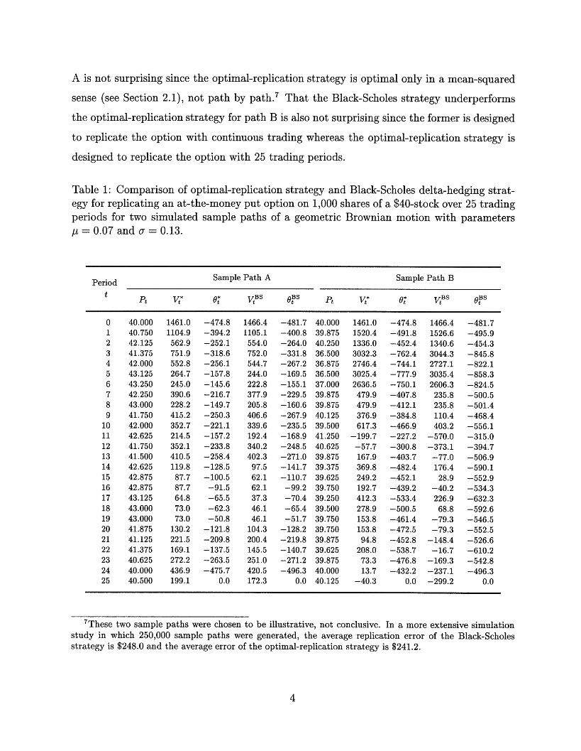
A is not surprising since the optimal-replication strategy is optimal only in a mean-squared
sense (see Section 2.1), not path by path.7 That the Black-Scholes strategy underperforms
the optimal-replication strategy for path B is also not surprising since the former is designed
to replicate the option with continuous trading whereas the optimal-replication strategy is
designed to replicate the option with 25 trading periods.
Table 1: Comparison of optimal-replication strategy and Black-Scholes delta-hedging strat-egy for replicating an at-the-money put option on 1,000 shares of a $40-stock over 25 tradingperiods for two simulated sample paths of a geometric Brownian motion with parametersI = 0.07 and or = 0.13.
Period Sample Path A Sample Path B
t Pt * VBS oBS * VBS
0 40.000 1461.0 -474.8 1466.4 -481.7 40.000 1461.0 -474.8 1466.4 -481.71 40.750 1104.9 -394.2 1105.1 -400.8 39.875 1520.4 -491.8 1526.6 -495.92 42.125 562.9 -252.1 554.0 -264.0 40.250 1336.0 -452.4 1340.6 -454.33 41.375 751.9 -318.6 752.0 -331.8 36.500 3032.3 -762.4 3044.3 -845.84 42.000 552.8 -256.1 544.7 -267.2 36.875 2746.4 -744.1 2727.1 -822.15 43.125 264.7 -157.8 244.0 -169.5 36.500 3025.4 -777.9 3035.4 -858.36 43.250 245.0 -145.6 222.8 -155.1 37.000 2636.5 -750.1 2606.3 -824.57 42.250 390.6 -216.7 377.9 -229.5 39.875 479.9 -407.8 235.8 -500.58 43.000 228.2 -149.7 205.8 -160.6 39.875 479.9 -412.1 235.8 -501.49 41.750 415.2 -250.3 406.6 -267.9 40.125 376.9 -384.8 110.4 -468.4
10 42.000 352.7 -221.1 339.6 -235.5 39.500 617.3 -466.9 403.2 -556.111 42.625 214.5 -157.2 192.4 -168.9 41.250 -199.7 -227.2 -570.0 -315.012 41.750 352.1 -233.8 340.2 -248.5 40.625 -57.7 -300.8 -373.1 -394.713 41.500 410.5 -258.4 402.3 -271.0 39.875 167.9 -403.7 -77.0 -506.914 42.625 119.8 -128.5 97.5 -141.7 39.375 369.8 -482.4 176.4 -590.115 42.875 87.7 -100.5 62.1 -110.7 39.625 249.2 -452.1 28.9 -552.916 42.875 87.7 -91.5 62.1 -99.2 39.750 192.7 -439.2 -40.2 -534.317 43.125 64.8 -65.5 37.3 -70.4 39.250 412.3 -533.4 226.9 -632.318 43.000 73.0 -62.3 46.1 -65.4 39.500 278.9 -500.5 68.8 -592.619 43.000 73.0 -50.8 46.1 -51.7 39.750 153.8 -461.4 -79.3 -546.520 41.875 130.2 -121.8 104.3 -128.2 39.750 153.8 -472.5 -79.3 -552.521 41.125 221.5 -209.8 200.4 -219.8 39.875 94.8 -452.8 -148.4 -526.622 41.375 169.1 -137.5 145.5 -140.7 39.625 208.0 -538.7 -16.7 -610.223 40.625 272.2 -263.5 251.0 -271.2 39.875 73.3 -476.8 -169.3 -542.824 40.000 436.9 -475.7 420.5 -496.3 40.000 13.7 -432.2 -237.1 -496.325 40.500 199.1 0.0 172.3 0.0 40.125 -40.3 0.0 -299.2 0.0
7 These two sample paths were chosen to be illustrative, not conclusive. In a more extensive simulationstudy in which 250,000 sample paths were generated, the average replication error of the Black-Scholesstrategy is $248.0 and the average error of the optimal-replication strategy is $241.2.
4

For sample path A, the differences between the optimal-replication strategy and the
Black-Scholes are not great-Vt* and O are fairly close to their Black-Scholes counterparts.
However, for sample path B, where there are two large price movements, the differences
between the two replication strategies and the replication errors are substantial. Even in
such an idealized setting, the optimal-replication strategy can still play an important role in
the dynamic hedging of risks.
In Section 2 we introduce the dynamic replication problem and propose a solution based
on stochastic dynamic programming. In Section 3 we recast the dynamic replication problem
under the equivalent martingale measure, which generalizes the typical derivative pricing and
hedging results to dynamically incomplete markets. The scope of the e-arbitrage approach
is illustrated in Sections 4 and 5 analytically and numerically for several examples including
path-dependent options and options on assets with mixed jump-diffusion and stochastic-
volatility price dynamics. The sensitivity of the replication error to price dynamics is studied
in Section 6, and we conclude in Section 7.
2 -Arbitrage Strategies
In this section, we formulate and propose a solution approach for the problem of option
pricing in incomplete markets. In Section 2.1 we introduce the replication problem and the
principle of e-arbitrage. In Sections 2.2 and 2.3 we propose stochastic dynamic programming
algorithms in discrete and continuous time, respectively.
2.1 The Dynamic Replication Problem
Consider an asset with price Pt at time t where 0 t < T and let F(PT, ZT) denote the
payoff of some European derivative security at maturity date T which is a function of PT and
other variables ZT (see below). For expositional convenience, we shall refer to the asset as a
stock and the derivative security as an option on that stock, but our results are considerably
more general.
As suggested by Merton's (1973) derivation of the Black-Scholes formula, the dynamic
replication problem is to find a dynamic portfolio strategy-purchases and sales of stock and
riskless borrowing and lending-on [0, T] that is self-financing and comes as close as possible
5
to the payoff F(PT, ZT) at T. To formulate the dynamic replication problem more precisely,
we begin with the following assumptions:
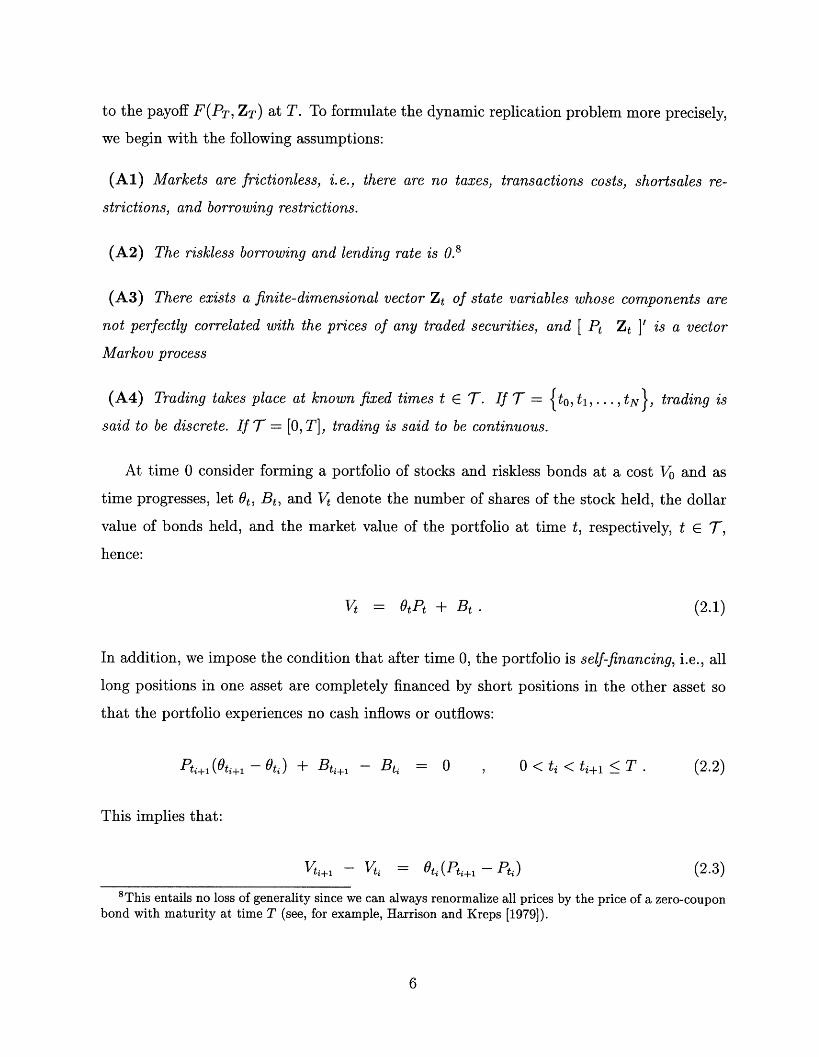
(Al) Markets are frictionless, i.e., there are no taxes, transactions costs, shortsales re-
strictions, and borrowing restrictions.
(A2) The riskless borrowing and lending rate is 0.8
(A3) There exists a finite-dimensional vector Zt of state variables whose components are
not perfectly correlated with the prices of any traded securities, and [ Pt Zt ]' is a vector
Markov process
(A4) Trading takes place at known fixed times t E T. If T = {to , t,..., tN }, trading is
said to be discrete. If T = [0, T], trading is said to be continuous.
At time 0 consider forming a portfolio of stocks and riskless bonds at a cost V and as
time progresses, let t, Be, and Vt denote the number of shares of the stock held, the dollar
value of bonds held, and the market value of the portfolio at time t, respectively, t E T,
hence:
t = OtPt + Bt. (2.1)
In addition, we impose the condition that after time 0, the portfolio is self-financing, i.e., all
long positions in one asset are completely financed by short positions in the other asset so
that the portfolio experiences no cash inflows or outflows:
Pt+( (0ti+ - ti) + Bt+l1 - Btj = 0 , 0 < t i < ti+ < T . (2.2)
This implies that:
Vti+ - Vti = Oti(Pti+1 Pti) (2.3)
8 This entails no loss of generality since we can always renormalize all prices by the price of a zero-couponbond with maturity at time T (see, for example, Harrison and Kreps [1979]).
6

and, in continuous time,
dVt = OtdPt. (2.4)
We seek a self-financing portfolio strategy {Ot}, t E T, such that the terminal value VT
of the portfolio is as close as possible to the option's payoff F(PT, ZT). Of course, there
are many ways of measuring "closeness", each giving rise to a different dynamic replication
problem. For reasons that will become clear shortly (see Sections 2.4 and 3), we choose a
mean-squared-error loss function, hence our version of the dynamic replication problem is:9
min E [VT - F(PT, ZT) (2.5)
subject to self-financing condition (2.3) or (2.4), the dynamics of [ Pt Zt ]', and the initial
wealth V0, where the expectation E" is taken with respect to a probability measure v that
represents the randomness of the difference VT - F(PT, ZT), conditional on information at
time 0.10
A natural measure of the success of the optimal-replication strategy is the square root of
the mean-squared replication error (2.5) evaluated at the optimal {Ot}, hence we define
E(VO) _0mi } E"{[VT- F(PT, ZT)]2 } (2.6)
We shall show below that (Vo) can be minimized with respect to the initial wealth V0 to
yield the least-cost optimal-replication strategy and a corresponding measure of the minimum
9Other recent examples of the use of mean-squared-error loss functions in related dynamic-trading prob-lems include Duffie and Jackson (1990), Duffie and Richardson (1991), Schil (1994), and Schweizer (1992,1995).
10Note that we have placed no constraints on {Ot}, hence it is conceivable that for certain replicationstrategies, VT is negative with positive probability. Imposing constraints on {0t} to ensure the non-negativityof VT would render the dynamic replication problem (2.5) intractable. However, negative values for VT is notnearly as problematic in the context of the dynamic replication problem as it is for the optimal consumptionand portfolio problem of, for example, Merton (1971). In particular, VT does not correspond to an individual'swealth, but is the terminal value of a portfolio designed to replicate a particular payoff function. See Dybvigand Huang (1988) and Merton (1992, Chapter 6) for further discussion.
7

replication error *:
E* - min E(Vo) . (2.7)
In the case of Black and Scholes (1973) and Merton (1973), there exists dynamic replication
strategies for which e* = 0, hence we say that perfect arbitrage pricing holds.
But there are situations-dynamically incomplete markets, for example-where perfect
arbitrage pricing does not hold. In particular, assumption (A3), the presence of state vari-
ables Zt that are not perfectly correlated with the prices of any traded securities, is the
source of market incompleteness in our framework. While this captures only one potential
source of incompleteness-and does so only in a "reduced-form" sense-nevertheless, it is a
particularly relevant source of incompleteness in financial markets. Of course, we recognize
that the precise nature of incompleteness, e.g., institutional rigidities, transactions costs,
technological constraints, will affect the pricing and hedging of derivative securities in com-
plex ways.1" Nevertheless, how well one security can be replicated by sophisticated trading
in other securities does provide one measure of the degree of market incompleteness even if
it does not completely characterize it. In much the same way that the Black and Scholes
(1973) and Merton (1973) models focus on the relative pricing of options-relative to the ex-
ogenously specified price dynamics for the underlying asset-we hope to capture the degree
of relative incompleteness, relative to an exogenously specified set of Markov state variables
that are not completely hedgeable.
In some of these cases, we shall show in Sections 2.2 and 2.3 that -arbitrage pricing is
possible, i.e., it is possible to derive a mean-square-optimal dynamic replication strategy that
is able to approximate the terminal payoff F(PT, ZT) of an option to within e*. But before
turning to the solution of the dynamic replication problem, we provide several illustrative
examples that delineate the scope of our framework.
1 1For more "structural" models in which institutional sources of market incompleteness are studied, e.g.,transactions costs, shortsales constraints, undiversifiable labor income, see Aiyagari (1994), Aiyagari andGertler (1991), He and Modest (1995), Heaton and Lucas (1992, 1996), Lucas (1994), Scheinkman and Weiss(1986), Telmer (1993), and Weil (1992). See Magill and Quinzii (1996) for a comprehensive analysis ofmarket incompleteness.
8
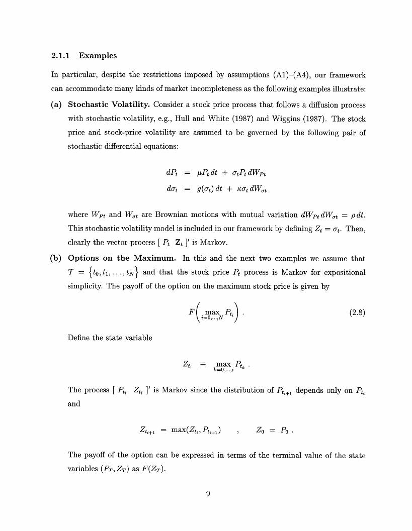
2.1.1 Examples
In particular, despite the restrictions imposed by assumptions (A1)-(A4), our framework
can accommodate many kinds of market incompleteness as the following examples illustrate:
(a) Stochastic Volatility. Consider a stock price process that follows a diffusion process
with stochastic volatility, e.g., Hull and White (1987) and Wiggins (1987). The stock
price and stock-price volatility are assumed to be governed by the following pair of
stochastic differential equations:
dPt = APt dt + tPt dWpt
dat = g(at) dt + sat dWat
where Wpt and W,t are Brownian motions with mutual variation dWpt dWt = p dt.
This stochastic volatility model is included in our framework by defining Zt = t. Then,
clearly the vector process [ Pt Zt ]' is Markov.
(b) Options on the Maximum. In this and the next two examples we assume that
T = {to, t 1 ,...,tN} and that the stock price Pt process is Markov for expositional
simplicity. The payoff of the option on the maximum stock price is given by
(mai= x ,. Pt) (2.8)
Define the state variable
Zti max Ptkk=O,...,i
The process [ Pti Zti ]' is Markov since the distribution of Pt,+, depends only on Pt,
and
Zti+l = max(Zti,Pti+l) Zo = Po
The payoff of the option can be expressed in terms of the terminal value of the state
variables (PT, ZT) as F(ZT).
9
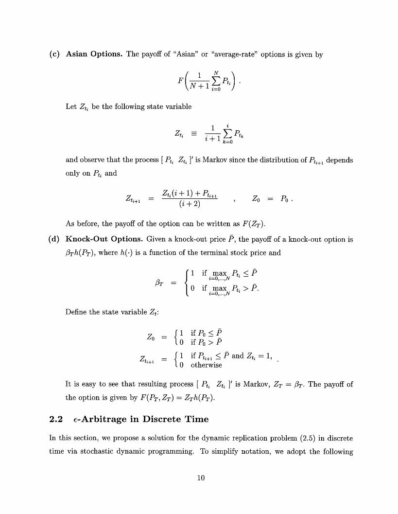
(c) Asian Options. The payoff of "Asian" or "average-rate" options is given by
F(N + iZe Pti )
Let Zti be the following state variable
_ 1 zti 1 E Ptk
k=O
and observe that the process [ Pti Zti ]' is Markov since the distribution of Pti+ depends
only on Pti and
Zti(i + 1) + Pti+1(i+2)
Zo = Po.
As before, the payoff of the option can be written as F(ZT).
(d) Knock-Out Options. Given a knock-out price P, the payoff of a knock-out option is
P3Th(PT), where h(-) is a function of the terminal stock price and
T = 0if max Pt < P
i=O,...,N
if max Pt > P.i=O,...,N
Define the state variable Zt:
Zo = 1 ifP o > P
zti+ = {1 ifPti+, < P and Zti = 1,0 otherwise
It is easy to see that resulting process [ Pti Zti ]' is Markov, ZT = T. The payoff of
the option is given by F(PT, ZT) = ZTh(PT).
2.2 e-Arbitrage in Discrete Time
In this section, we propose a solution for the dynamic replication problem (2.5) in discrete
time via stochastic dynamic programming. To simplify notation, we adopt the following
10
Zti+l

convention for discrete-time quantities: time subscripts ti are replaced by i, e.g., the stock
price Pti will be denoted as Pi and so on. Under this convention, we can define the usual
cost-to-go or value function Ji as:
Ji(vi, ,Zi) - min E [[VN - F(PN, ZN)] 2 V, Pi, Zi] (2.9)0(k,Vk,Pk,Zk),
i<k<N-1
where Vi, Pi, and Zi comprise the state variables, Oi is the control variable, and the self-
financing condition (2.3) and the Markov property (A3) comprise the law of motion for the
state variables. By applying Bellman's principle of optimality recursively (see, for example,
Bertsekas [1995]):
JN(VN, PN, ZN) = [VN - F(PN, ZN)] 2 (2.10)
Ji(V, Pi, Zi) = min E [ Ji+l(V+l, Pi, Zi+l) jV,P, Zi ]
i= 0,..., N- 1 (2.11)
the optimal-replication strategy O*(i, Vi, Pi, Zi) can be characterized and computed. In par-
ticular, we have:1 2
Theorem 1 Under Assumptions (A1)-(A4) and (2.3), the solution of the dynamic replica-
tion problem (2.5) for T = {to, tl,..., tN} is characterized by the following:
(a) The value function Ji(Vi, Pi, Zi) is quadratic in V, i.e., there are functions ai(Pi, Zi),
bi(Pi, Zi), and ci(Pi, Zi) such that
Ji(Vi, Pi, Zi) = ai(Pi, Zi). [Vi-bi(Pi, i O ... , N . (2.12)
(b) The optimal control O*(i, Vi, Pi, Zi) is linear in Vi, i.e.,
0*(i, i, Pi, Zi) = pi(Pi,Zi) - Vqi(P,Zi) (2.13)
12Proofs are relegated to the Appendix.
11
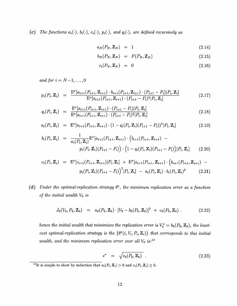
(c) The functions ai(.), bi(.), ci(.), Pi(.), and qi(), are defined recursively as
aN(PN, ZN) = 1 (2.14)
bN(PN, ZN)
Ci(PN, ZN)
= F(PN, ZN)
= 0
Ev[ai+l(Pi+l, Zi+l) bi+l(Pi+l, Zi+l) (Pi+ - Pi)lPi, Zi]
Ev[ai+l(Pi+l, Zi+l) · (Pi+ - Pi)21Pi, Zi]
E[ai+l(Pi+l, Zi+l) · (Pi+l - Pi)jPi, Zi]EV[ai+l(Pi+l, Zi+1 ) (Pi+ 1 - Pi)21Pi, Zi]
= EV[ai+l(Pi+l, Zi+l) (1 - qi(Pi, Zi)(Pi+l - P)) 21Pi, Zi]
- (P, Ev[ai+((Pi+, Zi+) (bi+1(Pi+, Zi+) -
Pi(Pi, Zi)(Pi+l - Pi)) (1 - qi(Pi, Zi)(Pi+1 - P.))IP Zi]
= Ev[ci+(Pi+, Zi+)lPi, Zi] + E"[ai+l(Pi+l, Zi+l) (bi+l(Pi+l, Zi+l) -
Pi(Pi, Z)(i+1 - P2))2 1P, Zi)(Pi+l - (Pi, Zi]) - i(Pi, Zi,)2 (2.21)
(d) Under the optimal-replication strategy 0*, the minimum replication error as a function
of the initial wealth Vo is
Jo(Vo, Po, Zo) = ao(Po, Zo) [Vo - bo(Po, Zo)]2 + co(P, ZO)
hence the initial wealth that minimizes the replication error is VO* = bo(Po, Zo), the least-
cost optimal-replication strategy is the {*(i, Vi, Pi, Zi)} that corresponds to this initial
wealth, and the minimum replication error over all Vo is:13
* = C(Po, Zo)
13It is simple to show by induction that ai(Pi, Zi) > 0 and ci(Pi, Zi) > 0.
(2.23)
12
and for i = N-1,...,0
(2.15)
(2.16)
pi(Pi, Zi)
qi(Pi, Zi)
ai(Pi, Zi)
bi(Pi, Zi)
(2.17)
(2.18)
(2.19)
ci(Pi, Z i)
(2.20)
(2.22)
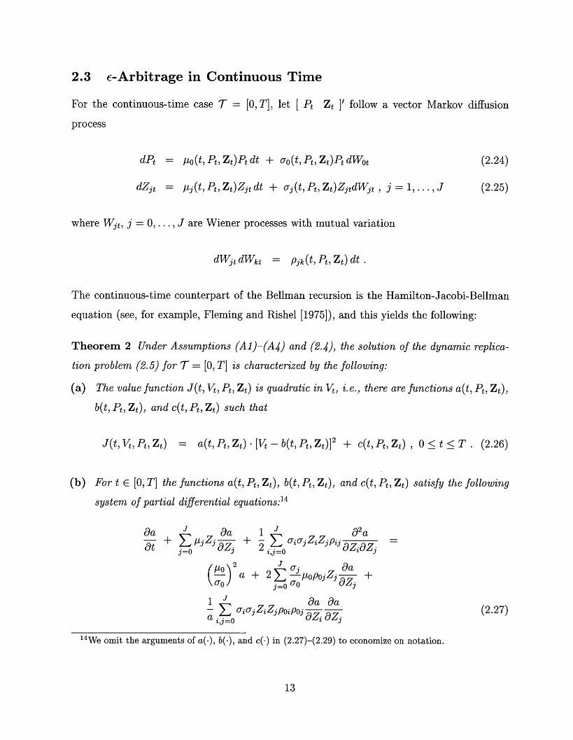
2.3 e-Arbitrage in Continuous Time
For the continuous-time case T = [0, T], let [ Pt Zt ]' follow a vector Markov diffusion
process
dPt = o(t, Pt, Zt)Pt dt + ao(t, Pt, Zt)Pt dWot (2.24)
-= gj(t, Pt, Zt)Zjt dt + aj(t, Pt, Zt)ZjtdWjt , j = 1,... , J
where Wjt, j = 0, ... , J are Wiener processes with mutual variation
dWjt dWkt = Pkc(t, Pt, Zt) dt.
The continuous-time counterpart of the Bellman recursion is the Hamilton-Jacobi-Bellman
equation (see, for example, Fleming and Rishel [1975]), and this yields the following:
Theorem 2 Under Assumptions (A1)-(A4) and (2.4), the solution of the dynamic replica-
tion problem (2.5) for 7 = [0, T] is characterized by the following:
(a) The value function J(t, Vt, Pt, Zt) is quadratic in Vt, i.e., there are functions a(t, Pt, Zt),
b(t, Pt, Zt), and c(t, Pt, Zt) such that
= a(t, Pt, Zt) [Vt - b(t, Pt, Z)] 2 + c(t, Pt, Zt), 0 • t < T (2.26)
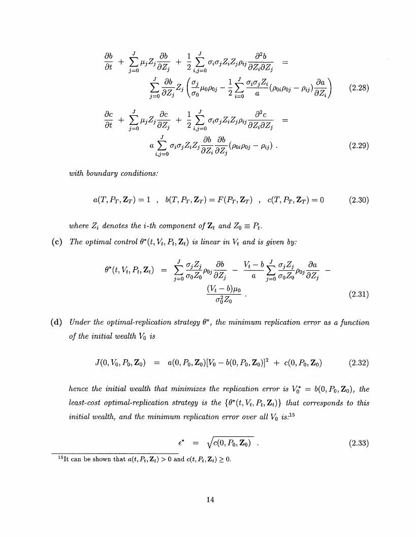
(b) For t E [0, T] the functions a(t, Pt, Zt), b(t, Pt, Zt), and c(t, Pt, Zt) satisfy the following
system of partial differential equations:1 4
12
Oa J Oa- + E j Zj
j=O 9J i,j=o a t 3
(Ao 2 + 2io a +/ a + 2 E topoJZj- +0j=0 o O Zj
a J -a aE -i a Zi Z; Po i AZ A (2.27)
14We omit the arguments of a(-), b(.), and c(.) in (2.27)-(2.29) to economize on notation.
13
dZjt (2.25)
i(t, Vt' Pt, Zt)
AQ2 -t
Ob + 3 aj=O aj
j Zj Z0j=o 9
ac + E ZIL aJj=0
1 J 02 b
i,j=o iZii Zj
I aiajZ (PoiPoji=O a
1 J 02 C+ - Z coijZiZjPii
2ij=O )ZiOZJ
ii a (Ob Oba ,Ez, Zo z-o-d--(PoiPoj - Pj)i,j=o aZ i azj
a(T, PT, ZT) = 1 , b(T, PT, ZT) = F(PT, ZT) C(T, PT, ZT) =
where Zi denotes the i-th component of Zt and Zo Pt.
(c) The optimal control 0*(t, Vt, Pt, Zt) is linear in Vt and is given by:
J Zj ob. ;oPO J ObZj=OcaoZo OZ -
(V - b)oUO
Vt - b J ajZj aa j=o a-ozopO azj
(2.31)
(d) Under the optimal-replication strategy 0*, the minimum replication error as a function
of the initial wealth Vo is
J(o, Vo, Po, Zo) = a(O, Po, Zo)[Vo - b(o, Po, Zo)] + c(0, Po, Zo)
hence the initial wealth that minimizes the replication error is VO* = b(O, Po, Zo), the
least-cost optimal-replication strategy is the {O*(t, Vt, Pt, Zt)} that corresponds to this
initial wealth, and the minimum replication error over all V is:15
E* = C(0o,Po, Zo) (2.33)
> 0 and c(t, Pt, Zt) > 0.
14
(2.28)
with boundary conditions:
(2.29)
(2.30)
(2.32)
1 5It can be shown that a(t, Pt, Zt)
01 OI0L P0 paz
O (t, Vt, Pt, Zt)

2.4 Interpreting e* and V*
Theorems 1 and 2 show that the dynamic replication problem (2.5) can be solved for a mean-
squared-error measure of replication error under Markov state dynamics. In particular, the
optimal-replication strategy 0*(.) is a dynamic trading strategy that yields the minimum
mean-squared replication error e(V0) for an initial wealth V0. The fact that (Vo) depends on
V0 should come as no surprise, and the fact that (V0 ) is quadratic in Vo emphasizes the fact
that delta-hedging strategies can be under- or over-capitalized, i.e., there exists a unique V0*
that minimizes the mean-squared replication error. One attractive feature of our approach
is the ability to quantify the impact of capitalization Vo on the replication error (V0).
2.4.1 V0* Is Not a Price
In this sense, V0* may be viewed as the minimum production-cost of replicating the payoff
F(PT, ZT) as closely as possible, to within e*. However, because we have assumed that
markets are dynamically incomplete (otherwise e* is 0 and perfect replication is possible),
V0* cannot be interpreted as the price of a derivative security with payoff F(PT, ZT) unless
additional economic structure is imposed. In particular, in dynamically incomplete mar-
kets derivatives cannot be priced by arbitrage considerations alone-we must resort to an
equilibrium model in which the prices of all traded assets are determined by supply and
demand.
To see why V0* cannot be interpreted as a price, observe that two investors with different
risk preferences may value F(PT, ZT) quite differently, and will therefore place different
valuations on the replication error e*. While both investors may agree that V0* is the minimum
cost for the optimal-replication strategy 0*(.), they may differ in their willingness to pay such
a cost for achieving the replication error *.16 Moreover, some investors' preferences may
not be consistent with a symmetric loss function, e.g., they may value negative replication
errors quite differently than positive replication errors.
More to the point, an asset's price is the outcome of a market equilibrium in which
investors' preferences, budget dynamics, and information structure interact through the im-
position of market-clearing conditions, i.e., supply equals demand. In contrast, V0* is the
16See Duffie and Jackson (1990) and Duffie and Richardson (1991) for examples of replication strategiesunder specific preference assumptions.
15
solution to a simple dynamic optimization problem that does not typically incorporate any
notion of economic equilibrium. However, in Section 3 we modify the dynamic optimization
problem to account for such equilibrium considerations, and the V0* that solves this modi-
fied optimal-replication problems does correspond to the equilibrium price of the derivative
security (see Theorem 3).
2.4.2 Why Mean-Squared Error?
In fact, there are many possible loss functions, each giving rise to a different set of dynamic
replication strategies, hence a natural question to ask in interpreting Theorems 1 and 2 is
why use mean-squared error?
The first reason is, of course, tractability. We showed in Sections 2.2 and 2.3 that
the dynamic replication problem can be solved via stochastic dynamic programming for a
mean-squared-error loss function and Markov state dynamics, and that the solution can be
implemented as an exact and efficient recursive algorithm. In Sections 4 and 5, we apply
this algorithm to a variety of derivative securities in incomplete markets and demonstrate
its practical relevance analytically and numerically.
The second reason is that a symmetric loss function is the most natural choice when we
have no prior information about whether the derivative to be replicated is being purchased
or sold. In such cases, asymmetric loss functions are inappropriate since positive replication
errors for a long position become negative replication errors for the short position. Indeed,
when a derivatives broker is asked by a client to provide a price quote, the client does
not reveal whether he is a buyer or seller until after he receives both bid and offer prices.
Therefore, it is in the interest of the broker to provide as "tight" a spread as possible, i.e.,
to minimize mean-squared error.
Of course, in more structured applications such as Duffie and Jackson (1990) in which
investors' preferences, budget dynamics, and information sets are specified, it is not ap-
parent that mean-squared-error optimal-replication strategies are optimal from a particular
investor's point of view. However, even in these cases, a slight modification of the mean-
squared-error loss function yields optimal-replication strategies that have natural economic
interpretations. In particular, we show in the next section that by defining mean-squared
16
error with respect to equivalent martingale measure, the minimum production cost V0* as-
sociated with this loss function can be interpreted as an equilibrium market price which,
by definition, incorporates all aspects of the economic environment in which the derivative
security is traded. This is the third and perhaps the most compelling motivation for a
mean-squared error loss function.
3 Risk-Neutralized -Arbitrage Strategies
To relate the minimum production cost V* of the optimal-replication strategy to the market
price of a derivative security with payoff F(PT, ZT), in this section we propose a minor
but important modification to the dynamic replication problem (2.5) of Section 2. The
modification consists of evaluating the mean-squared replication error with respect to an
adjusted probability measure v*-the risk-neutralized or equivalent martingale measure-
hence the risk-neutralized dynamic replication problem becomes:
min E* {[VT - F(PT, ZT)] 2). (3.1)
Although (3.1) seems virtually identical to (2.5), the implications of using v* in place of v are
significant. In Section 3.1, we show that the minimum production cost V0* associated with
(3.1) does correspond to the equilibrium price of a derivative security with payoff F(PT, ZT),
and is not merely a "proxy" for the price. As a consequence, the algorithm of Theorems
1 and 2 provides an explicit optimal dynamic replication strategy that corresponds to the
equilibrium price of the derivative security, which complements the standard delta-hedging
strategies and generalizes them to an incomplete-markets setting.
Of course, v* is not always readily observable and additional structure is needed to infer
v* from existing market prices-we discuss this issue in Section 3.2.
3.1 Equilibrium Pricing Models and -Arbitrage
In Section 2.4 we argued that the minimum production cost V0* cannot be interpreted as
the price of a derivative security with payoff F(PT, ZT) because EV[VT - F(PT, ZT)]2 does
not necessarily reflect an investor's preferences regarding the replication error. To derive
17
the equilibrium price of the derivative security, we require additional economic structure,
i.e., investors' preferences, budget dynamics, information structure, and the imposition of
market-clearing conditions.
Such economic structure is summarized by the equivalent martingale measure v*, also
known as the state-price density or the risk-neutral density. Cox and Ross (1976) and
Harrison and Kreps (1979) show that under certain regularity conditions, the equilibrium
prices of all traded securities must be martingales under this adjusted probability measure,
hence the price of any security can be determined simply as the expectation of its payoff,
where the expectation is evaluated with respect to v*.1 7 Therefore, if H(O, Po, Z0) denotes
the equilibrium market price of the option at time 0, then
H(0, Po, Z o) = E [F(PT, ZT)] . (3.2)
But observe that an implication of minimizing mean-squared error (3.1) is that:1 8
E* [VT - F(PT, ZT)] = 0 (3.3)
where V denotes the terminal value of the portfolio under the optimal replicating strategy
0* (.). Since the optimal-replication strategy is self-financing so that there are no cash inflows
or outflows during the interval (0, T), it must be the case that V0* = EV* [V]. This in turn
implies:
V = EV*[VT*] = EV [F(PT,ZT)] = H(0,Po,Z0o). (3.4)
Therefore, we have:
Theorem 3 Under Assumptions (A1)-(A4) and (2.3) or (2.4), the minimum production
cost Vo* corresponding to the risk-neutralized dynamic replication problem (3.1) is the equi-
librium price of a derivative security with payoff F(PT, ZT).
Observe that Theorem 3 does not assume dynamically complete markets, unlike the
17See Duffie (1996), Duffie and Huang (1985), Huang (1987), Huang and Litzenberger (1988), and Merton(1992) for further details.
18 See, for example, Schweizer (1995).
18
standard arbitrage-based pricing model of Merton (1973). Therefore, when v* is substituted
for v in Theorems 1 and 2, the recursive algorithms outlined in those two theorems yield
risk-neutralized optimal-replication strategies that generalize the standard Merton (1973)
delta-hedging strategies to dynamically incomplete markets. Hereafter, we shall refer to
0*(.) under v* as a generalized delta-hedging strategy.
3.2 How to Obtain v*
While Theorem 3 seems to suggest that the generalization of delta-hedging to dynamically
incomplete markets is straightforward-substitute v* for v--obtaining v* can often be quite
a challenge. In a dynamic equilibrium model such as Lucas (1978) and Rubinstein (1976),
the equivalent martingale measure is a weighted average of the probability measure v, where
the weighting function is the equilibrium marginal rate of substitution of the representative
agent. This dynamic equilibrium interpretation illustrates the enormous information content
of v* and the enormous information reduction that the equivalent martingale measure affords.
Indeed, from a pricing perspective, v* is a "sufficient statistic" in the sense that it contains
all relevant information about preferences and business conditions for purposes of pricing
financial securities.
But as a practical matter, how does one obtain v* to make Theorems 1-3 operational?
There are at least two possible approaches to this challenge-theoretical and empirical-and
we shall describe each of these in the next two sections.
3.2.1 Theoretical Methods
The theoretical approach is to provide sufficient economic structure, i.e., a fully articulated
dynamic equilibrium model as in Cox, Ingersoll, and Ross (1985), to yield a unique v*. In
such an environment, using v* leads to a significant simplification of the dynamic replication
problem. For example, consider a continuous-time model in which stock prices and the state
variables Zt are described by the following system of Markov diffusion processes:
dPt = [to(t,Pt,Zt)Ptdt + o(t,Pt,Zt)PtdWot
dZjt = ,j(t,Pt, Zt)Zjtdt + j(t,Pt, Zt)ZjtdWjt , j = 1,. .. ,J
19

Under the risk-neutral measure v*, the risk-neutralized drift rate /ut(t, Pt, Zt) becomes:
O (t Pt, Zt) = 0
while the diffusion coefficients remain unchanged. This simplifies the system of PDE's (2.27)-
(2.29) to:
a(t, Pt, Zt) = 1 (3.5)
Ob(t, Pt, Zt) J ab(t, Pt, Zt) 1 ZjPij2b(t, Pt, Zt)
t ,,/LZj +Zj + 2 aijo - 0 (3.6)at j=1 zij=oazazj
ac(t, Pt, Zt) J Oc(t Pt Zt) 1 2c(t, Pt, Zt)at + t 3 anz + 2 ZiPij azaz3j=1 3 j=o
I; ¢o ab(t, Pt, Zt) ob(t, P, Zt)Z ai ZTZ azi az (POiPoj - Pij) (3.7)
i,j=O zi
and the optimal number of shares in the replicating portfolio is given by:19
ab(t, Pt, Zt) J aj Zj a(t, P, z,)*(t, t, t, t) - bP + Ad 3 PoZ az (3.8)OZO j=1 oZo aZj
Interestingly, the optimal replicating strategy 0*(t, Vt, Pt, Zt) depends on the equivalent
martingale measure v* only indirectly, through the option price H(t, Pt, Zt) = b(t, Pt, Zt).
In other words, all information necessary for the construction of the optimal replicating
strategy is contained in the option price itself. Moreover, the optimal replicating strategy
is independent of the value of the portfolio Vt. These are properties of the delta-hedging
strategies of arbitrage-based models such as Merton (1973), and they carry through to the
generalized delta-hedging strategies of e-arbitrage models as well.
Indeed, in addition to the term ab(t, Pt, Zt)/aZo which is the well-known Black-Scholes
hedge ratio, the generalized delta-hedging strategy *(t, Vt, Pt, Zt) contains additional terms
19(3.8) follows from (4.4) in Schweizer (1992), which was obtained under a set of assumptions differentfrom those adopted in the present paper. The results in Schweizer (1992) do not apply to the case when theobjective function is defined using the original probability measure v, but they are applicable here since thedrift rate of the stock price process under the equivalent martingale measure is equal to zero.
20
of the form Ob(t, Pt, Zt)/OZj, that use changes in the stock price to hedge against changes in
the non-traded state variables Zj. These terms are weighted by the correlation coefficients
(ajZj/oZo)poj, that determine the degree to which such a hedging is effective. To see that
(3.8) is a direct generalization of the Black and Scholes (1973) and Merton (1973) delta-
hedging formula, observe that it reduces to the Black and Scholes (1973) and Merton (1973)
option delta when the state variables Zj are instantaneously uncorrelated with the stock
price.
3.2.2 Empirical Methods
An alternative to developing a fully articulated dynamic equilibrium model is to estimate v*
from the prices of existing financial securities. This is the approach taken in several recent
papers, including Ait-Sahalia and Lo (1996), Derman and Kani (1994), Dumas et al. (1995),
Dupire (1994), Hutchinson et al. (1994), Jarrow and Rudd (1982), Longstaff (1992, 1995),
Rady (1994), Rubinstein (1994), and Shimko (1993).
For example, AYt-Sahalia and Lo (1996) propose a nonparametric method for estimating
v*: construct a nonparametric estimator of a call-option pricing formula using market prices,
then take the second derivative of the estimated pricing formula with respect to the strike
price. Banz and Miller (1978), Breeden and Litzenberger (1978), and Ross (1976) show that
this second derivative is v*.
Another method for determining v* empirically is Rubinstein's (1994) implied binomial
tree, in which the risk-neutral probabilities {i7r } associated with the binomial terminal stock
price PT are estimated by minimizing the sum of squared deviations between {ir)} and a
set of prior risk-neutral probabilities {i}), subject to the restrictions that {7r* } correctly
price an existing set of options and the underlying stock [in the sense that the optimal risk-
neutral probabilities yield prices that lie within the bid-ask spreads of the options and the
stock]. This approach is similar in spirit to Jarrow and Rudd (1982) and Longstaff's (1992,
1995) method of fitting risk-neutral density functions using a four-parameter Edgeworth
expansion.20
20 However, Rubinstein (1994) points out several important limitations of Longstaff's method when ex-tended to a binomial model, including the possibility of negative probabilities. See, also, Derman and Kani(1994), Shimko (1993), Dupire (1994), and Dumas et al. (1995)].
21

Once v* has been estimated, a numerical implementation of the recursive algorithms in
Theorems 1 and 2 can be undertaken. We hope to examine the properties of such procedures
in future research.
4 Illustrative Examples
To illustrate the scope and power of the -arbitrage approach to the dynamic replication
problem, we apply the results of Section 2 to four specific cases for the return-generating
process: state-independent returns (Section 4.1), geometric Brownian motion (Section 4.2),
a jump-diffusion model (Section 4.3), and a stochastic volatility model (4.4).
4.1 State-Independent Returns
Suppose that stock returns are state-independent so that
Pi = Pi-1 (1 + i-1 ) (4.1)
where i-l is independent of the current stock price and all other state variables. This,
together with the Markov assumption (A3) implies that returns are statistically indepen-
dent (but not necessarily identically distributed) through time. Also, let the payoff of the
derivative security F(PT) depend only on the price of the risky asset at time T.
In this case, there is no need for additional state variables Zi and the expressions in
Theorem 1 simplify to:
aN = 1 , bN(PN) = F(PN) , CN(PN) = 0 (4.2)
and for i = N-1,...,0,
2
ai = ai+l (4.3)=7 + [4?
bi(Pi) = E' [bi+l(P(1 +- i))lPi] Cov [i, bi+l(Pi( + i))IPi] (4.4)
ci(Pi) = E' [ci+l(Pi(l + qi))Pi] + a{o2Varv[bi+1 (Pi(1 + ))IPi] -
22

Cov [i, bj+j(Pi(l + ij))Pi]2 } (4.5)
Pi(Pi) EV [ibi+l(Pi(1 + cfi))Pi] (4.6)(ai + Dip
qi(Pi) = ( 2 + (4.7)
where i = Ev[0i] and a2 = Varv[0i].
4.2 Geometric Brownian Motion
Let the stock price process follow the geometric Brownian motion of Black and Scholes (1973)
and Merton (1973). We show that the e-arbitrage approach yields the Black-Scholes/Merton
results in the limit of continuous time, but in discrete time there are important differences be-
tween the optimal-replication strategy of Theorem 1 and the standard Black-Scholes/Merton
delta-hedging strategy.
For notational convenience, let all discrete time intervals [ti, ti+l) be of equal length
ti+l -ti = At. The assumption of geometric Brownian motion then implies:
Pi+ = Pi ( + i) (4.8)
log(1 + Xi) = ( - 2 )At + JaAtzi (4.9)
i - (0, 1). (4.10)
Recall that for At << 1 (a large number of time increments on [0, T]), the following approx-
imation holds (see, for example, Merton [1992, Chapter 3]):
Xi ,J \ (lAt, U2 t) + (At 3/2)
This, and Taylor's theorem, imply the following approximations for the recursive relations
(4.3)-(4.5) of Section 4.1:
VarV[bi+l(Pi(1 + qi))IPi] = bi+ (Pi)2Pi2At O (t 2 )
23
Cov [i, bi+l(Pi(1 + 0i))lPi] = bi+l(Pi)z2 PiAt + O(At2 )
E[bi+l(Pi(1 + i))Pi] = bi+l(Pi) + bil(Pi)P zt +' ' i2 + O(At2 )
E[ ci+(P(1 +i))P/] = cil(Pi)mPj/t + ci) 1(P) 2 it + +l(Pi- O(t 2).
We can then rewrite (4.4)-(4.5) as
2
b,(P,) = b,±(P) + b+,(P,) 2 't + O(At2)bi(Pi) = bi+1(Pi) + 2 + (Pi)
ci(Pi) ci+j(i) Ci+l(pil)/PitAt Ci+l(Pi) At + O(t 2 )
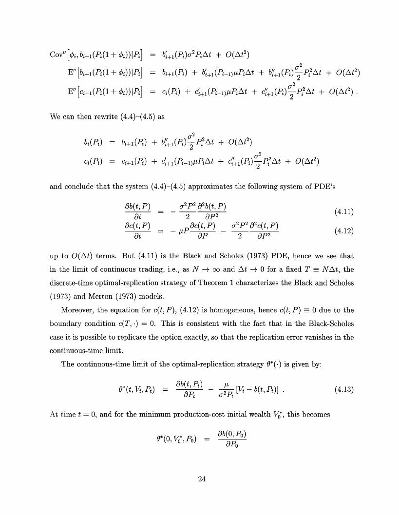
and conclude that the system (4.4)-(4.5) approximates the following system of PDE's
Ob(t, P) o2 P2 02b(t, F) (4.11)at = - 2 0P (4.11)at 2 aP 2
ac(t, P) = POac(t,P) 22 2C(t, p)(4.12)at a= 2 oP2
up to O(At) terms. But (4.11) is the Black and Scholes (1973) PDE, hence we see that
in the limit of continuous trading, i.e., as N -+ oo and At -+ 0 for a fixed T _ NAt, the
discrete-time optimal-replication strategy of Theorem 1 characterizes the Black and Scholes
(1973) and Merton (1973) models.
Moreover, the equation for c(t, P), (4.12) is homogeneous, hence c(t, P) 0 due to the
boundary condition c(T, ) = 0. This is consistent with the fact that in the Black-Scholes
case it is possible to replicate the option exactly, so that the replication error vanishes in the
continuous-time limit.
The continuous-time limit of the optimal-replication strategy 0*(-) is given by:
*(t, Vt,Pt) ab(t, P) a [Vt - b(t, Pt)] . (4.13)ap (t Pt) ·
At time t = 0, and for the minimum production-cost initial wealth VO*, this becomes
0* (OVo*, Po) ab(0, P0)ap0
24
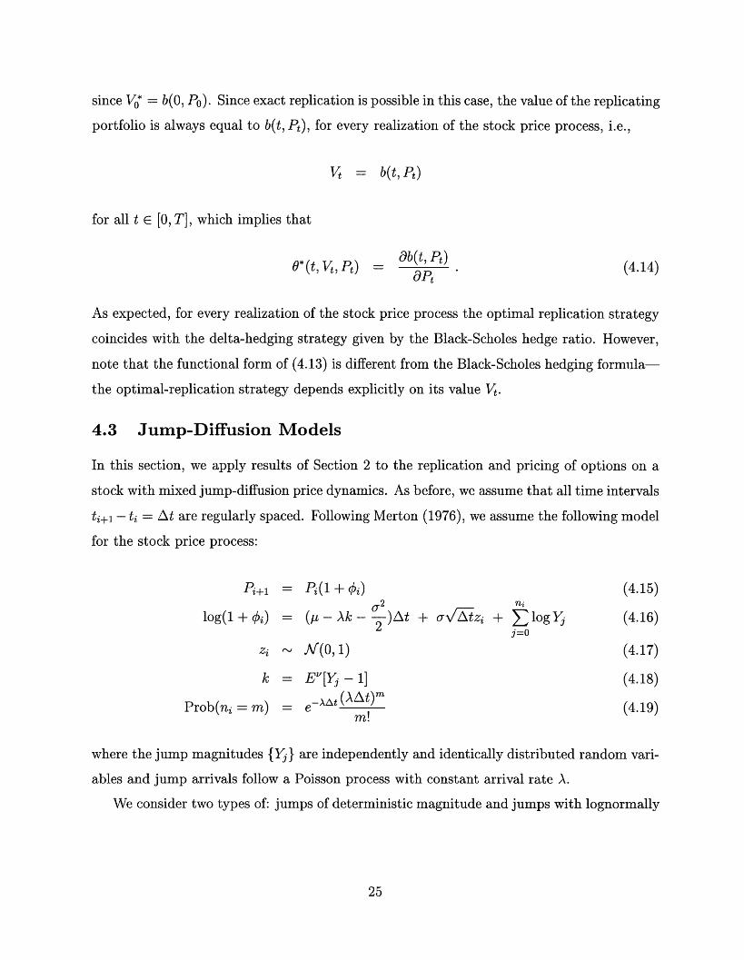
since VO* = b(O, PO). Since exact replication is possible in this case, the value of the replicating
portfolio is always equal to b(t, Pt), for every realization of the stock price process, i.e.,
Vt = b(t,Pt)
for all t E [0, T], which implies that
*(t, Vt, Pt) = b(t,Pt) (4.14)
As expected, for every realization of the stock price process the optimal replication strategy
coincides with the delta-hedging strategy given by the Black-Scholes hedge ratio. However,
note that the functional form of (4.13) is different from the Black-Scholes hedging formula
the optimal-replication strategy depends explicitly on its value Vt.
4.3 Jump-Diffusion Models
In this section, we apply results of Section 2 to the replication and pricing of options on a
stock with mixed jump-diffusion price dynamics. As before, we assume that all time intervals
ti+l- ti = At are regularly spaced. Following Merton (1976), we assume the following model
for the stock price process:
Pi+l = Pi(1 + i) (4.15)0-2 ni
log(1 + i) = (u-Ak- -2 )At + oa/zi + logYj (4.16)j=o
zi A(0O, 1) (4.17)
k = Ev[Yj-1] (4.18)
Prob(ni = m) = e - ,t (AAt) m (4.19)m!
where the jump magnitudes {Yj} are independently and identically distributed random vari-
ables and jump arrivals follow a Poisson process with constant arrival rate A.
We consider two types of: jumps of deterministic magnitude and jumps with lognormally
25

distributed jump magnitudes. In the first case:
Y = 1 + . (4.20)
If we set = 0 in (4.15), this model corresponds to the continuous-time jump process
considered by Cox and Ross (1976). In the second case:
logYi .- A/(0,,62). (4.21)
There are two methods of calculating the optimal-replication strategy for the mixed jump-
diffusion model. One method is to begin with the solutions of the dynamic programming
problem given in Sections 2.2 and 2.3, derive a limiting system of partial differential equations
as in Section 4.2, and solve this system numerically, using one of the standard finite difference
schemes.
The second method is to implement the solution of the dynamic programming problem
directly, without the intermediate step of reducing it to a system of PDE's.
The advantage of the second method is that it treats a variety of problems in a uniform
fashion, the only problem-dependent part of the approach being the specification of the
stochastic process. On the other hand, the first approach yields a representation of the solu-
tion as a system of PDE's, which can often provide some information about the qualitative
properties of the solution even before a numerical solution is obtained.
With these considerations in mind, we shall derive a limiting system of PDE's for the
deterministic-jump-magnitude specification (4.20) and use it to find conditions on the pa-
rameters of the stochastic process which allow exact replication of the option's payoff, or,
equivalently, arbitrage pricing. For the lognormal-jump-magnitude specification (4.21), we
shall obtain numerical solutions directly from the dynamic programming algorithm of The-
orem 1.
26
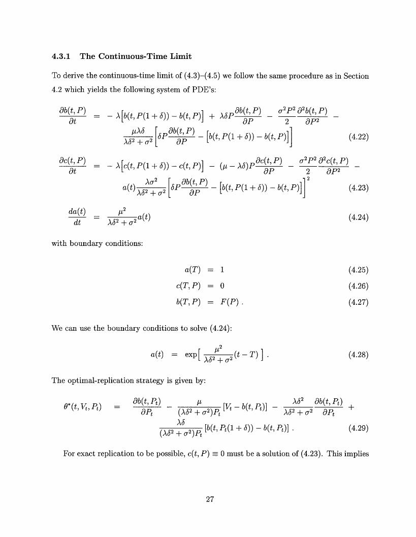
4.3.1 The Continuous-Time Limit
To derive the continuous-time limit of (4.3)-(4.5) we follow the same procedure as in Section
4.2 which yields the following system of PDE's:
- A [b(t, P(1 + )) - b(t, P)]
pAb(t, P)OPA62 + 2 6
+ Apb(t, P) a 2 P2 d 2b(t, P)P 2 OP2
[b(t, P(1 + 6)) - b(t, P)]]
= - A [c(t, P(1 + 6)) - c(t, P)] - ( - ,,)Pac(t, P)- (p-A6P
u 2P2 02C(t, P)2 aP2
a(t) A 2+ a(t) A6 2 + o-2 P(1 + 6)) -
(4.24)L2A2 + a
with boundary conditions:
a(T)
c(T, P)
b(T, P)
= 1
= 0
= F(P).
We can use the boundary conditions to solve (4.24):
a(t) = exp[ A2 2 (t - T) ] .
The optimal-replication strategy is given by:
=Ob(t, Pt) A [t - b(t, Pt)]Opt (A62 -+ 2)Pt
62 + [b(t, Pt( + ))(AJ2 U2)Pt
A62 Ob(t, Pt)A62 + 2 dPt
- b(t, P)]
For exact replication to be possible, c(t, P) - 0 must be a solution of (4.23). This implies
27
Ob(t, P)at
ac(t, P)at
(4.22)
da(t)dt
b(t, P)]] (4.23)
(4.25)
(4.26)
(4.27)
o*(t, Vt, P)
(4.28)
+
(4.29)
[6P Ob(t, P) - [b(t,
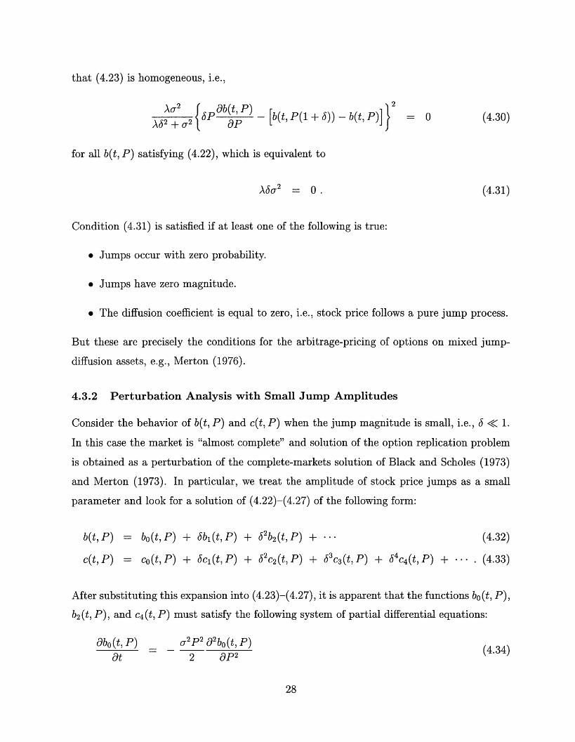
that (4.23) is homogeneous, i.e.,
AU2+ p Ob(t, P)_ [b(t, P(1 6)) b)]1 = 0 (4.30)A62 + 2 + P
for all b(t, P) satisfying (4.22), which is equivalent to
A6U2 = 0. (4.31)
Condition (4.31) is satisfied if at least one of the following is true:
* Jumps occur with zero probability.
* Jumps have zero magnitude.
* The diffusion coefficient is equal to zero, i.e., stock price follows a pure jump process.
But these are precisely the conditions for the arbitrage-pricing of options on mixed jump-
diffusion assets, e.g., Merton (1976).
4.3.2 Perturbation Analysis with Small Jump Amplitudes
Consider the behavior of b(t, P) and c(t, P) when the jump magnitude is small, i.e., < 1.
In this case the market is "almost complete" and solution of the option replication problem
is obtained as a perturbation of the complete-markets solution of Black and Scholes (1973)
and Merton (1973). In particular, we treat the amplitude of stock price jumps as a small
parameter and look for a solution of (4.22)-(4.27) of the following form:
b(t, P) = bo(t,P) + bl (t, P) + 2 b2(t,P) + ... (4.32)
c(t,P) = co(t,P) + cl(t,P) + 62c2 (t, P) + 63 c3 (t, P) + 64 c4 (t, P) + .... (4.33)
After substituting this expansion into (4.23)-(4.27), it is apparent that the functions bo(t, P),
b2 (t, P), and c4 (t, P) must satisfy the following system of partial differential equations:
db0o(t, P) O-2 P 2 02bo(t, P)(4.34)at 2 aP 2
28

ab2(t, P)at
Oc4(t, P)at
AP 2 02bo(t, P)2 aP2
dc4(t, P) 2P2 02c 4(t, P) _ AP4 02bo(t, P) 2- ip - 2 P2 a(t 4 aP 2 aP 2 4 ap 2
with boundary conditions:
bo(T, P)
b2(T, P)
c4 (T, P)
= F(P)
= 0
= 0
and
bl = cl = C2 = c3 = O
System (4.34)-(4.39) can be solved to yield:
b(t, P) = bo(t,P) + 2 [bo(t, P) - F(P)] + 0(63)aT
where bo0(t, P) is the option price in the absence of a jump component, i.e., the Black-Scholes
formula in the case of put and call options. Observe that for an option with a convex payoff
function bo(t, P) > F(P), which implies that b(t, P) > bo(t, P), i.e., the addition of a small
jump component to geometric Brownian motion increases the price of the option. This
qualitative behavior of the option price is consistent with the results in Merton (1976) which
were obtained with equilibrium arguments.
The optimal-replication strategy (4.29) is given by:
abo(tI Pt) Ab+ , + [bo(t, Pt) - Vt] +ap cr2 Pt
A62 bo (t, Pt) _F(Pt) + V-F(Pt)o-2 OPt aPt t
+ 0(63). (4.41)
29
(4.35)
(4.36)
(4.37)
(4.38)
(4.39)
(4.40)
0 (t, V P)

and the corresponding replication error is:
c(t, P) = 64c4(t, P) + 0(66) = (4) (4.42)
where c4 (t, P) solves (4.36) and (4.39).
Equations (4.40) and (4.41) provide closed-form expressions for the replication cost and
the optimal-replication strategy when the amplitude of jumps is small, i.e., when markets
are almost complete, and (4.42) describes the dependence of the replication error on the
jump magnitude.
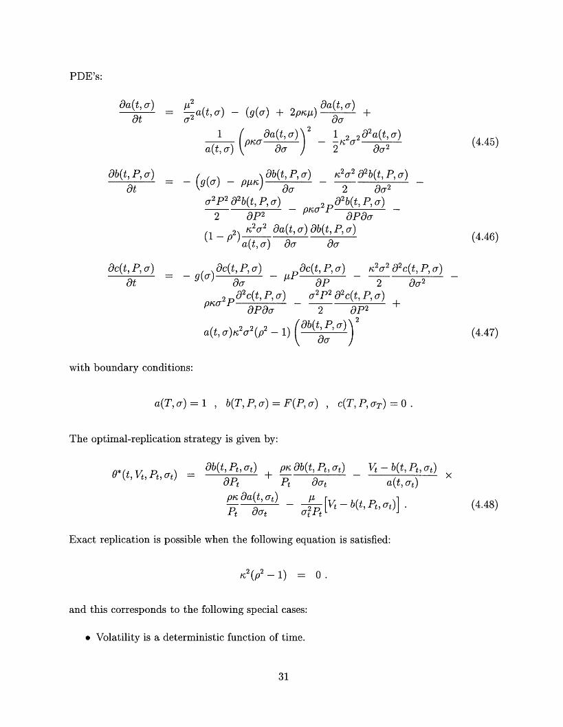
4.4 Stochastic Volatility
Let stock prices follow a diffusion process with stochastic volatility as in Hull and White
(1987) and Wiggins (1987):
dPt = zPtdt + tPtdWpt (4.43)
drt = g(at)dt + ratdWt (4.44)
where Wpt and Wt are Brownian motions with mutual variation dWptdWat = pdt.
4.4.1 The Continuous-Time Solution
Although applying the results of Section 2 to (4.43)-(4.44) is conceptually straightforward,
the algebraic manipulations are quite involved in this case. A simpler alternative to deriving
a system of PDE's as the continuous-time limit of the solution in Theorem 1, we formulate
the problem in continuous time at the outset and solve it using continuous-time stochastic
control methods. This approach simplifies the calculations considerably.
Specifically, the pair of stochastic processes (Pt, at) satisfies assumptions of Section 2.3,
therefore results of this section can be used to derive the optimal-replication strategy, the
minimum production-cost of optimal replication, and the replication error. In particular,
the application of the results of Section 2.3 to (4.43)-(4.44) yields the following system of
30
A~2= 2 a(t, ) -
1
a(t, a)
(g(O) + 2p) Oaa(t, )19U
(KU a(t, a )2 1 2 2 02a(t, or )
2 022 a
= - (g(c) - pl) ab(t, P
r2P2 02b(t, P, (J)
2 aP2
a) _ 2a 2 92 b(t, P, a) _
2 O02
a2 2b(t, P, ) _pK aPaCP
ac(t, P, ) at
ac(t, P, a)
aP
a(t, a) 2 2 (p2
Oc(t, P, U) _K 2U2 a2 C(t, P, U)
dP 2 a 2
a) 2 2 a2 C(t, p,U)
cr 2 aP2
_)( b(t, P, r)
with boundary conditions:
a(T, ) = 1 b(T, P, ) = F(P, a) , c(T,P, aT)= O .
The optimal-replication strategy is given by:
o*(t, Vt, Pt, at) ab(t, Pt, at)aPtpK aa(t,Pt a
pK ab(t, Pt, at)
Pt artat) [
t aat Lt
Vt- b(t, Pt, t)
a(t, t)
b(t,Pt, at)]
Exact replication is possible when the following equation is satisfied:
K2 (p 2 1) = 0.
and this corresponds to the following special cases:
* Volatility is a deterministic function of time.
31
PDE's:
aa(t, )at
ab(t, P, a)
at
(4.45)
2K2 aa(t, a) ab(t, P, )a(t, a) aa ac (4.46)
(4.47)
x
(4.48)

* The Brownian motions driving stock prices and volatility are perfectly correlated.
Both of these conditions yield well-known special cases where arbitrage-pricing is possible
(see, for example, Geske [1979] and Rubinstein [1983]). If we set ti = g(a) = 0, (4.46) reduces
to the Black and Scholes (1973) PDE.
5 Numerical Analysis
The essence of the -arbitrage approach to the dynamic replication problem is the recogni-
tion that although perfect replication may not be possible in some situations, the optimal-
replication strategy of Theorem 1 may come very close. How close is, of course, an empirical
matter hence in this section we present several numerical examples that complement the
theoretical calculations of Section 4.
In Section 5.1 we describe our numerical procedure and implement it for following ex-
amples: geometric Brownian motion (Section 5.2), a mixed jump-diffusion model with a
lognormal jump magnitude (Section 5.3), and a stochastic volatility model (Section 5.4).
In addition, we also implement our numerical solution algorithm for a stochastic volatility
model under an equivalent martingale measure in Section 5.5. Finally, in Section 5.6 we
apply our algorithm to the path-dependent option to "sell at the high".
5.1 The Numerical Procedure
To implement the solution (2.17)-(2.21) of the dynamic replication problem numerically, we
begin by representing the functions ai(P, Z), bi(P, Z), and ci(P, Z) by their values over a
spatial grid {(pi, Zk) : j = 1,..., J, k = 1,...,. K}. For any given (P,Z), values ai(P, Z),
bi(P, Z), and ci(P, Z) are obtained from ai(P, Zk), bi(Pj , Zk), and ci (Pi, Zk) using a piece-
wise quadratic interpolation. This procedure provides an accurate representation of ai(P, Z),
bi(P, Z), and ci(P, Z) with a reasonably small number of sample points. The values ai(Pj, Zk),
bi(Pj , Zk), and ci(pi, Zk) are updated according to the recursive procedure (2.17)-(2.19).
We evaluate the expectations in (2.17)-(2.19) by replacing them with the corresponding
integrals. For all the models considered in this paper, these integrals involve Gaussian
kernels. We use Gauss-Hermite quadrature formulas (see, for example, Stroud [1971]) to
obtain efficient numerical approximations of these integrals.
32

In all cases except for the path-dependent options, we perform numerical computations
for a European put option with a unit strike price (K = 1), i.e., F(PT) = max(0, K-PT),
and a six-month maturity. It is apparent from (2.17)-(2.21) that for a call option with the
same strike price K, the replication error ci(.) is the same as that of a put option, and the
replication cost bi(.) satisfies the put-call parity relation. We assume 25 trading periods,
defined by to = 0, ti+l- ti = At = 1/50.
(a) (b)
Stock Price Stock Price
Figure 1: The difference between the replication cost and the intrinsic value of a six-monthmaturity European put option, plotted as a function of the initial stock price. The stockprice follows a geometric Brownian motion with parameter values = 0.07 and a = 0.13corresponding to the solid line. In Panel (a), [t is varied and is fixed; in Panel (b), -is varied and L is fixed. In both cases, the variation in each parameter is obtained bymultiplying its original value by 1.25 (dashed-dotted line), 1.5 (dots), 0.75 (dashed line) and0.5 (pluses).
5.2 Geometric Brownian Motion
Let stock prices follow a geometric Brownian motion, which implies that returns are lognor-
mally distributed as in (4.8)-(4.10). We set L- = 0.07 and a = 0.13, and to cover a range of
empirically plausible parameter values, we vary each parameter by increasing and decreasing
them by 25% and 50% while holding the values of other parameter fixed. Figure 1 displays
the minimum replication cost V0* minus the intrinsic value F(P0 ), for the above range of
parameter values, as a function of the stock price at time 0.
33
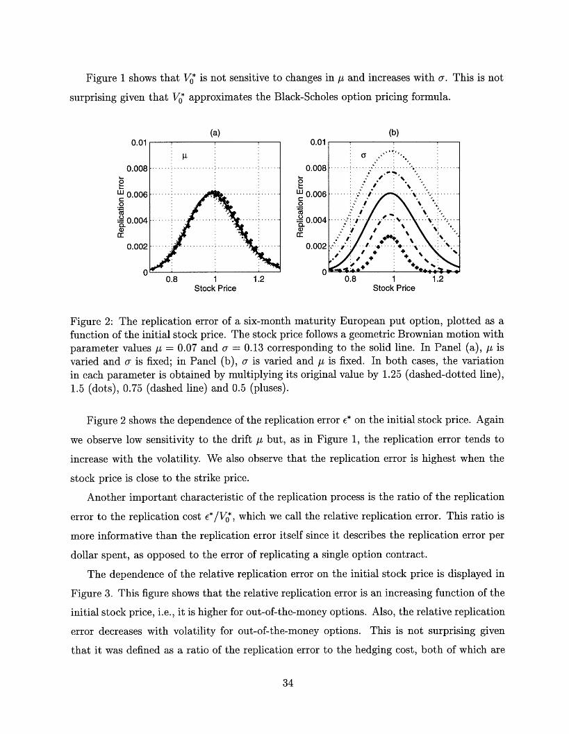
Figure 1 shows that V0* is not sensitive to changes in u and increases with a. This is not
surprising given that VO* approximates the Black-Scholes option pricing formula.
(a) (b)U.UI
0.008
0w 0.0060
=*0.004
cr0.002
n
V. I
0.008· ·
W 0.006 ...
0.004 · ·:
0.002 A d 4 44 44,
, .0.8 1 1.2 0.8 1 1.2
Stock Price Stock Price
Figure 2: The replication error of a six-month maturity European put option, plotted as afunction of the initial stock price. The stock price follows a geometric Brownian motion withparameter values , = 0.07 and or = 0.13 corresponding to the solid line. In Panel (a), / isvaried and oa is fixed; in Panel (b), is varied and /, is fixed. In both cases, the variationin each parameter is obtained by multiplying its original value by 1.25 (dashed-dotted line),1.5 (dots), 0.75 (dashed line) and 0.5 (pluses).
Figure 2 shows the dependence of the replication error e* on the initial stock price. Again
we observe low sensitivity to the drift /t but, as in Figure 1, the replication error tends to
increase with the volatility. We also observe that the replication error is highest when the
stock price is close to the strike price.
Another important characteristic of the replication process is the ratio of the replication
error to the replication cost c*/Vo*, which we call the relative replication error. This ratio is
more informative than the replication error itself since it describes the replication error per
dollar spent, as opposed to the error of replicating a single option contract.
The dependence of the relative replication error on the initial stock price is displayed in
Figure 3. This figure shows that the relative replication error is an increasing function of the
initial stock price, i.e., it is higher for out-of-the-money options. Also, the relative replication
error decreases with volatility for out-of-the-money options. This is not surprising given
that it was defined as a ratio of the replication error to the hedging cost, both of which are
34

increasing functions of volatility. According to this definition, the dependence of the relative
replic; ication
error;
(a) (b)
C0
Q.
._n-
cc
I
° 0.8wroc0.6.)U)
cc 0.4U)._
a) 0.2
n1 0.9 0.95 1 1.05 1.1
Stock Price Stock Price
Figure 3: The relative replication error of a six-month maturity European put option (relativeto the replication cost), plotted as a function of the initial stock price. The stock price followsa geometric Brownian motion with parameter values = 0.07 and a = 0.13 correspondingto the solid line. In Panel (a), is varied and a is fixed; in Panel (b), a is varied and / isfixed. In both cases, the variation in each parameter is obtained by multiplying its originalvalue by 1.25 (dashed-dotted line), 1.5 (dots), 0.75 (dashed line) and 0.5 (pluses).
5.3 Jump-Diffusion Models
Our numerical computations are based on the model (4.15)-(4.19), (4.21). In our numerical
implementation we restrict the number of jumps over a single time interval to be no more
than three, which amounts to modifying the distribution of ni in (4.16), originally given by
(4.19).21 Specifically, we replace (4.19) with
Prob[ni = m] = e - XAt (AA) m = 12, 3 (5.1)m!
3
Prob[ni = 0] = 1 - E Prob[ni = m] . (5.2)m=l
21 This "truncation problem" is a necessary evil in the estimation of jump-diffusion models. See Ball andTorous (1985) for further discussion.
35

(a) (b)0.05
,0 .0 4 ............... ................... o0.04
a 0.03 . . ...o o.20.02 0
00.8 0.9 1 1.1
Stock Price Stock Price
(c) (d)0.05
.0.040
0.03. 1.... .1
. 002
0.01
00.8 09 1 11
Stock Price Stock Price
Figure 4: The difference between the replication cost and the intrinsic valuef of a six-monthmaturity European put option, plotted as a function of the initial stock price. The stockprice follows the mixed jump-diffusion process given in (4.15)-(4.18), (4.21), (5.1), and (5.2)with parameter values g = 0.07, a = 0.106, A = 25, and 6 = 0.015 corresponding to the solidline. In Panels (a)-(d), , , A, and 6 are each varied, respectively, while the other parametervalues are held fixed. The variation in each parameter is obtained by multiplying its originalvalue by 1.25 (dashed-dotted line), 1.5 (dots), 0.75 (dashed line), and 0.5 (pluses).
36
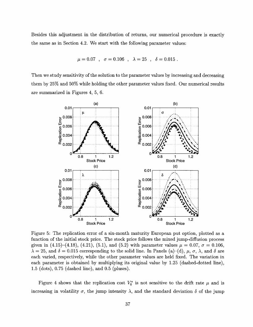
Besides this adjustment in the distribution of returns, our numerical procedure is exactly
the same as in Section 4.2. We start with the following parameter values:
/,=0.07 , = 0.106, A = 25 = 0.015.
Then we study sensitivity of the solution to the parameter values by increasing and decreasing
them by 25% and 50% while holding the other parameter values fixed. Our numerical results
are summarized in Figures 4, 5, 6.
(a))1
08
)6
)4 . . I\
)2 ....
ni' , 0.8 1
Stock Price
(c)
0.8 1Stock Price
0.01
0.0082
LUc 0.006o
.2 0.004
r 0.002
01.2
0.01
- 0.008P
a 0.006.o
.2 0.004a)
I 0.002
01.2
(b)
0.8 1 1.2Stock Price
(d)
I ;
:I ' : '
0.8 1 1.2Stock Price
Figure 5: The replication error of a six-month maturity European put option, plotted as afunction of the initial stock price. The stock price follows the mixed jump-diffusion processgiven in (4.15)-(4.18), (4.21), (5.1), and (5.2) with parameter values L = 0.07, = 0.106,A = 25, and 6 = 0.015 corresponding to the solid line. In Panels (a)-(d), [L, a, A, and 6 areeach varied, respectively, while the other parameter values are held fixed. The variation ineach parameter is obtained by multiplying its original value by 1.25 (dashed-dotted line),1.5 (dots), 0.75 (dashed line), and 0.5 (pluses).
Figure 4 shows that the replication cost V* is not sensitive to the drift rate L and is
increasing in volatility a, the jump intensity A, and the standard deviation 6 of the jump
37
O.C
0.0
C 0.Oc
c 0.0c
0.c
(7
...... , ...... ... ~,' ............
i \ ':-!i~~~~~~~~~' ',i"·r ~~~~~~~~~~~~~·
/4 ,'4 '4"I !~ 4= r
)1
0.00E
0.006
0.004
0.00d
I1
. .X
I......
. .. . ..... ..2 .1 . .
>, ... .. I........
0
o0.i.o
a)cc
rV
,_ _ , , , w ejU1
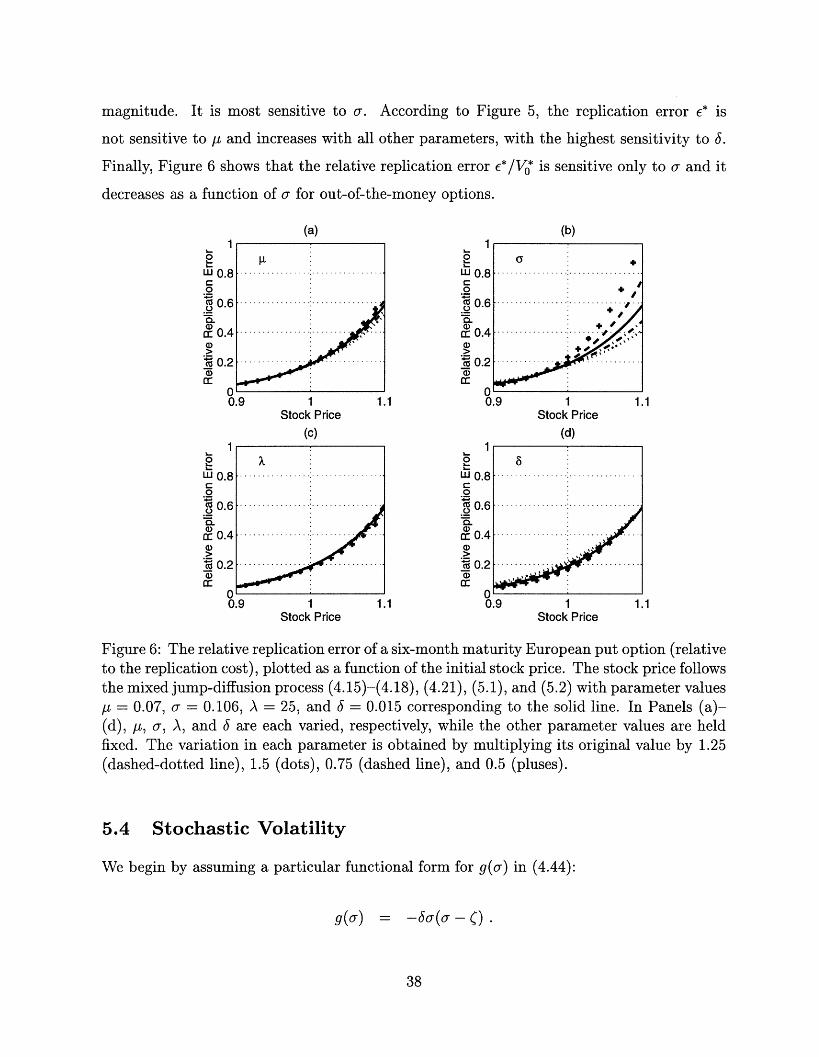
magnitude. It is most sensitive to . According to Figure 5, the replication error * is
not sensitive to ,L and increases with all other parameters, with the highest sensitivity to .
Finally, Figure 6 shows that the relative replication error e*/V0* is sensitive only to and it
decreases as a function of a for out-of-the-money options.
(a) (b)Ia
1
W 0.80
.X 0.6.6
r 0.4a
X 0.2
a
1
W 0.8C0
0.6
a 0.4
X 0.2
nFI
0.9 1 1.1
w
.oCg
n-a)
a)
a)
Stock Price Stock Price
(c) (d)
0LI
C.2
0.o
a)a)_c
0.9 1 1.1 0.9 1 1.1Stock Price Stock Price
Figure 6: The relative replication error of a six-month maturity European put option (relativeto the replication cost), plotted as a function of the initial stock price. The stock price followsthe mixed jump-diffusion process (4.15)-(4.18), (4.21), (5.1), and (5.2) with parameter valuesI = 0.07, = 0.106, A = 25, and 6 = 0.015 corresponding to the solid line. In Panels (a)-(d), IL, a, A, and 6 are each varied, respectively, while the other parameter values are heldfixed. The variation in each parameter is obtained by multiplying its original value by 1.25(dashed-dotted line), 1.5 (dots), 0.75 (dashed line), and 0.5 (pluses).
5.4 Stochastic Volatility
We begin by assuming a particular functional form for g(or) in (4.44):
g(cr) = -Ja(o- )
38
.4
)I
1

We also assume that the Brownian motions driving the stock price and volatility are un-
correlated. Since the closed-form expressions for the transition probability density of the
diffusion process with stochastic volatility are not available, we base our computations on
the discrete-time approximations of this process.22 The dynamics of stock prices and volatil-
0.05
c 0.03.o
.o 0.02a)
0.01
00
(b)
.8 0.9 1 1.1Stock Price
(d)0.05
4- V.V't
0c 0.03.o
.'o 0.020.
a- 0.01
n9 1 1.1Stock Price
0.8 0.'9 1 1.1Stock Price
Figure 7: The difference between the replication cost and the intrinsic value of a six-monthmaturity European put option, plotted as a function of the initial stock price. The stockprice follows the with stochastic volatility model (5.3)-(5.4) with parameter values It = 0.07,
= 0.153, 6 = 2, = 0.4, and 0 = 0.13 corresponding to the solid line. In Panels (a)-(d), , 6, , and o are each varied, respectively, while the other parameter values are heldfixed. The variation in each parameter is obtained by multiplying its original value by 1.25(dashed-dotted line), 1.5 (dots), 0.75 (dashed line), and 0.5 (pluses).
22 This is done mostly for convenience, since we could approximate the transition probability density usingMonte Carlo simulations. It should be pointed out that, while the discrete-time approximations lead tosignificantly more efficient numerical algorithms, they are also consistent with many estimation procedures,replacing continuous-time processes with their discrete-time approximations (see, for example, Ball andTorous [1985] and Wiggins [1987]).
39
0.05(a)
.0.................................
............. .............I... ...... """"
00
co
._
aDcc
0.04
0.03
0.02
0.01
.................................
....... ....... ..........
n0.8 0.9
- \ r,
1 1.13tock Price
(c)
....... ..........................
.. . . . .
A\ A- V.Vq'o00c 0.03o
.- 0.02Q.a)
n- 0.01
Av -0.8 O.
·2:'
I/: : : : : ' '''.. .; ' :'''
X _i \ '..... .,, ~.-. ';-
.
% t^A
U.UO
--I
A AA

ity are described by
Pi+ = Pi exp (( - oi2/2)At +- iVZp i ) (5.3)
=i+l = iexp ((--6( i - ) - 2/2)/At + Itczai) (5.4)
where zpi, zai -' KJ(0, 1) and E[zpizai] = 0. The parameters of the model are chosen to be
_= 0.07 , = 0.153 , =2 , = 0.4. (5.5)
We also assume that at time t = 0 volatility a0o is equal to 0.13. As before, we study
sensitivity of the solution to parameter values. Our findings are summarized in Figures 7, 8,
9.
We do not display the dependence on /u in these figures since the sensitivity to this
parameter is so low. Figure 7 shows that the replication cost is sensitive only to the initial
value of volatility ao and, as expected, the replication cost increases with a0. Figure 8
shows that the replication error is sensitive to rc and a0 and is increasing in both of these
parameters. According to Figure 9, the relative replication error is increasing in a. It also
increases in a 0 for in-the-money options and decreases for out-of-the-money options.
In addition its empirical relevance, the stochastic volatility model (4.43)-(4.44) also pro-
vides a clear illustration of the use of e* as a quantitative measure of dynamic market-
incompleteness. Table 2 reports the results of Monte Carlo experiments in which the optimal-
replication strategy is implemented for six sets of parameter values for the stochastic volatility
model, including the set that yields geometric Brownian motion.
For each set of parameter values, 1,000 independent sample paths of the stock price are
simulated, each sample path containing 25 observations, and for each path the optimal-
replication strategy is implemented. The averages (over the 1,000 sample paths) of the
minimum production cost V*, the realized replication error e*, the initial optimal stock
holdings 09, and the average optimal stock holdings * (over the 25 periods), is reported in
each row. For comparison, the theoretical replication error * is also reported.
Since stochastic volatility implies dynamically incomplete markets whereas geometric
Brownian motion implies the opposite, these six sets of simulations comprise a sequence of
40
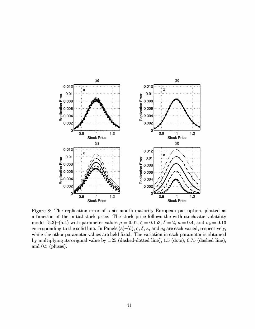
(a)
0.8 1 1.2Stock Price
(c)
0.8 1Stock Price
1.2
0.012
. 0.010
0.00E
0.006._a 0.004r
0.002
0.012
0 0.01LU 0.008
. 0.00E
-0.004
0.002
0J
0.8 1 1.2Stock Price
(d)
0.8 1Stock Price
1.2
Figure 8: The replication error of a six-month maturity European put option, plotted asa function of the initial stock price. The stock price follows the with stochastic volatilitymodel (5.3)-(5.4) with parameter values ,/ = 0.07, C = 0.153, = 2, r = 0.4, and oO = 0.13corresponding to the solid line. In Panels (a)-(d), (, 6, n, and u0 are each varied, respectively,while the other parameter values are held fixed. The variation in each parameter is obtainedby multiplying its original value by 1.25 (dashed-dotted line), 1.5 (dots), 0.75 (dashed line),and 0.5 (pluses).
41
0.012
i 0.010
w 0.008
* 0.006
Q 0.0040r
0.002
0.012
.. 0.010
J 0.008C
*. 0.006._o, 0.004
0.002
.................................
..........' ' A .. .....: K
i ! ,
4 ·\ · ··-; · ·
/ '~~
' '.. . ..... ../ .....
? .. .. '
· + "',2 · ,·-
. . . .
(b)
I
5
II
I
... . . .. . . . ... .. . . . . . . . . . .
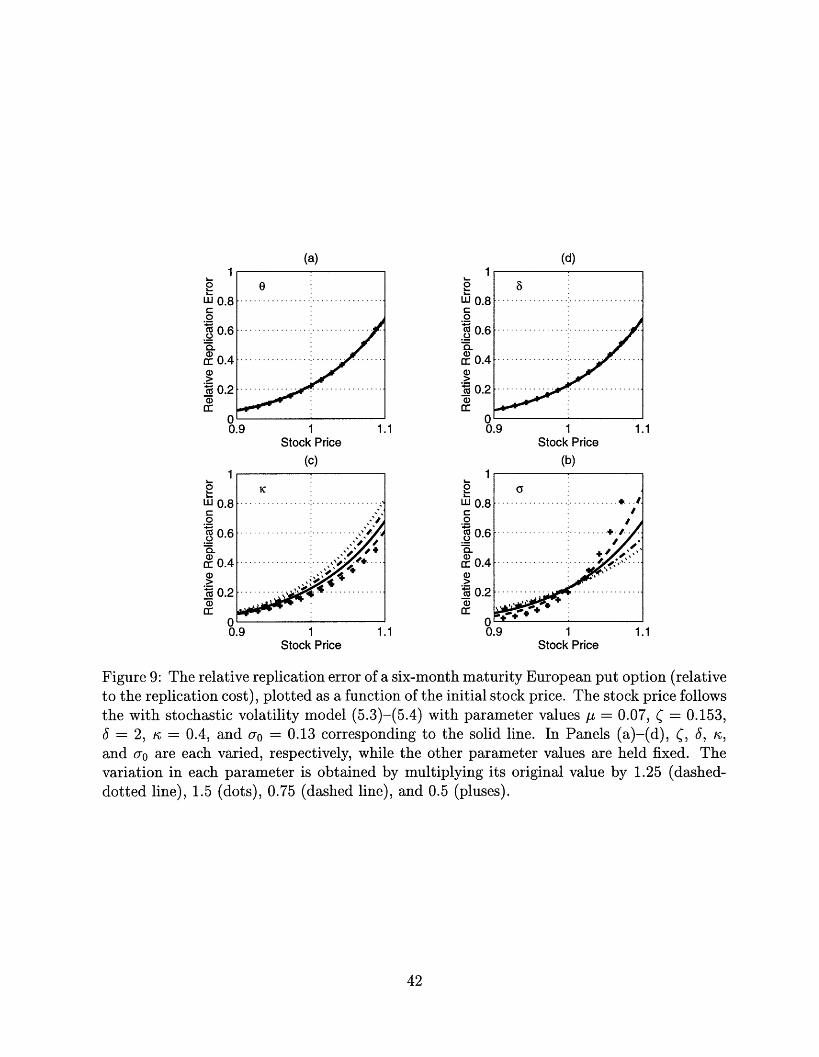
(a) (d)1 1~~~~~~~~~~~~
o
LU 0.8
0.40Cr 0.4
X 0.2
n
0o
C-
.o
.2_0n03c.
a)
a:
u0.9 1 1.1
0
rC.
i)
Q)n'
Stock Price Stock Price
(c) (b)
0
C
... ... .. ... .."/ao
0.9 1 1.1
1
1Stock Price Stock Price
Figure 9: The relative replication error of a six-month maturity European put option (relativeto the replication cost), plotted as a function of the initial stock price. The stock price follows
the with stochastic volatility model (5.3)-(5.4) with parameter values /u = 0.07, ( = 0.153,
a = 2, = 0.4, and ao = 0.13 corresponding to the solid line. In Panels (a)-(d), (, 6, ,and o are each varied, respectively, while the other parameter values are held fixed. The
variation in each parameter is obtained by multiplying its original value by 1.25 (dashed-
dotted line), 1.5 (dots), 0.75 (dashed line), and 0.5 (pluses).
42
0.................................
............................
................... .....
I. . .. .
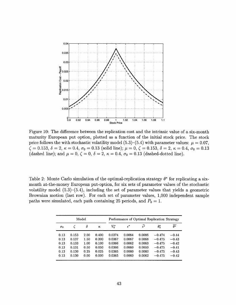
0.035
0.03
0tI
0.C)0
o0a)cca:
0.025
0.02
0.015
0.01
0.005
0.9 0.92 0.94 0.96 0.98 1 1.02 1.04 1.06 1.08 1.1Stock Price
Figure 10: The difference between the replication cost and the intrinsic value of a six-monthmaturity European put option, plotted as a function of the initial stock price. The stockprice follows the with stochastic volatility model (5.3)-(5.4) with parameter values: /t = 0.07,
= 0.153, 6 = 2, = 0.4, uo = 0.13 (solid line); /t = 0, = 0.153, 6 = 2, = 0.4, Oao = 0.13(dashed line); and /t = 0, ( = 0, 6 = 2, = 0.4, uo = 0.13 (dashed-dotted line).
Table 2: Monte Carlo simulation of the optimal-replication strategy 0* for replicating a six-month at-the-money European put-option, for six sets of parameter values of the stochasticvolatility model (5.3)-(5.4), including the set of parameter values that yields a geometricBrownian motion (last row). For each set of parameter values, 1,000 independent samplepaths were simulated, each path containing 25 periods, and P0 = 1.
Model Performance of Optimal Replication Strategy
a0 C a /C V * C e* 0 9*
0.13 0.153 2.00 0.400 0.0374 0.0084 0.0086 -0.474 -0.440.13 0.137 1.50 0.200 0.0367 0.0067 0.0068 -0.475 -0.430.13 0.133 1.00 0.100 0.0366 0.0062 0.0063 -0.475 -0.420.13 0.131 0.50 0.050 0.0366 0.0060 0.0059 -0.475 -0.410.13 0.130 0.25 0.025 0.0365 0.0060 0.0060 -0.475 -0.430.13 0.130 0.00 0.000 0.0365 0.0060 0.0062 -0.475 -0.42
43
::......... ......... :............ ...........
....... .................I ........... ..... ... ..'
...... ................
. .............../ :
.:,.: 4 i :
.4./., ..............
.4s'
I I I J ! I I I I I~~~~~~~~~~~~~~~~~~~~~~~~~~~~~~~~~~~~~~~~
I I
a----....... .......................... I.....
.... .-
.:. .. .
----: .. .. . I. I I I I
I
·...
: .%-:
.. ...... . .
I
': .......... :.........
models that illustrate the fact that market completeness need not be a binary characteristic.
In particular, Table 2 shows that as the parameter values move closer to geometric Brownian
motion, the average replication error e* decreases from 0.0086 to 0.0060. Moreover, the
decrease between the first and second rows is considerably larger than the decrease between
the second and third rows-the second and third rows imply price processes that are closer to
each other in their degree of market completeness than that of the first row. Such specific rank
orderings and sharp numerical comparisons are simply unavailable from standard dynamic
equilibrium models that have been used to model market incompleteness.
Of course, e* is only one of many possible measures of market incompleteness-a canonical
measure seems unlikely to emerge from the current literature-nevertheless it is an extremely
useful measure given the practical implications that it contains for dynamically hedging risks.
5.5 Stochastic Volatility Under The Risk-Neutral Measure
To study the effects of changing the original probability measure v to the risk-neutral proba-
bility measure v*, we consider the case when the stock price follows the stochastic volatility
process (5.3)-(5.4). Under the original probability measure v, we assume that parameters
of the model are:
= 0.07 , C=0.153 , =2 , = 0.4 , 0 =0.13. (5.6)
Under the risk-neutral probability measure v* the drift rate of the stock price is zero. To
define the process completely we need to specify the drift rate of the volatility under the new
measure. We consider two cases. In the first case the new (risk-adjusted) drift rate is equal
to the original drift rate, i.e., parameters and remain unchanged. In the second case we
assume that there exists a risk premium on the risk associated with the volatility process,
so that the risk-adjusted drift rate of this process is different from its original value. To be
specific, we leave unchanged and set = 0. Our results are summarized in Figure 10.
Figure 10 shows that the replication cost obtained by using the original probability
measure v is almost identical to the price of the option in case when volatility risk is not priced
by the market. On the other hand, when there exists a risk premium on the volatility risk,
the replication cost is different from exact price. The sign and magnitude of the difference
44

obviously depend on the exact form of the risk premium.
0.2
' 0.1500
= 0.1
Q
a: 0.05
n
(a)
0.8
I'llu./
t 0.15o0
0co0.
a)a: 0.05
n
0.9Stock Price
(c)
0.8 0.9Stock Price
0.2
o 0.150
o 0.1._
I: 0.05
rv-0.1
1
Cna:a0
(b)
8
0.80.8
0.9Stock Price
(d)
0.9Stock Price
1
Figure 11: The replication cost of a six-month maturity European option to "sell at thehigh", plotted as a function of the initial stock price. The stock price follows the mixedjump-diffusion process (4.15)-(4.18), (4.21), (5.1), and (5.2) with parameter values m = 1,/p = 0.07, = 0.106, A = 25, and = 0.015 corresponding to the solid line. In Panels(a)-(d), Ap, o, A, and 6 are each varied, respectively, while the other parameter values areheld fixed. The variation in each parameter is obtained by multiplying its original value by1.25 (dashed-dotted line), 1.5 (dots), 0.75 (dashed line), and 0.5 (pluses).
5.6 Path-Dependent Options
We consider the option to "sell at the high" as described by Goldman et al. (1979), under
the assumption that the stock price follows the mixed jump-diffusion process (4.15)-(4.18),
(4.21), (5.1), (5.2). We define the state variable Z:
Zo = m > Po
Zi+l = max(Zi,Pi+l)
45
g. .. ... ... ... ...
.. . . . . . .·.
. ... .. ... ... . . ... .. .
1
X 8............... 1.
. 11 ............I I "
:.............._

According to this definition, Zi is the running maximum of the stock price process at time
ti. The initial value of Zi is m, i.e., we assume that at time 0 the running maximum is equal
to m.
The payoff of the option is given by
F(PT,ZT) = ZT - PT
In our numerical analysis we set m = 1 as a convenient normalization. Note that this
convention is just a change of scale and does not lead to any loss of generality.
(a)
2 0.015UL
=0.01.o
0.00cc 0.00OE
rV0.8
U.UZ
o 0.015
Co 0.01
0.005Cc 0.005
r
0.9Stock Price
(c)
0.8 0.9Stock Price
0.02
O 0.015c
0* 0.01
.oa)
cc 0.005
n
(b)
... ,. . ...........,' a + -/+' "~" ."
'- +
0.9Stock Price
(d)
0.9Stock Price
0.8
8
1
0.02
2 0.015
C0.01
0.005cc 0.005
0.1
1
1
Figure 12: The replication error of a six-month maturity European option to "sell at thehigh", plotted as a function of the initial stock price. The stock price follows the mixedjump-diffusion process (4.15)-(4.18), (4.21), (5.1), and (5.2) with parameter values m = 1,
= 0.07, a = 0.106, A = 25, and 6 = 0.015 corresponding to the solid line. In Panels(a)-(d), g/, a, A, and 6 are each varied, respectively, while the other parameter values areheld fixed. The variation in each parameter is obtained by multiplying its original value by1.25 (dashed-dotted line), 1.5 (dots), 0.75 (dashed line), and 0.5 (pluses).
The parameters for the stock price process are taken to be the same as in Section (4.3).
46
..........................- ..... .11 ,+
. . .. . . . . ..;·Z
6
.. -' ~'' Xl
....... ........;~ .. --' 4
I
i
I
. .. ... ... .. .. ... ..I
.-:. .. ... ... . ...
I
n ,\rrV.VC.. U~..
5 .....
n
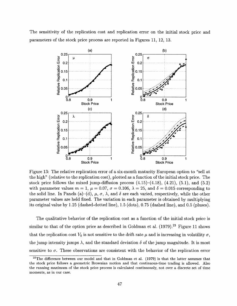
The sensitivity of the replication cost and replication error on the initial stock price and
parameters of the stock price process are reported in Figures 11, 12, 13.
(a) (b)V.Z0
g
U 0.2C
` 0.15
,)a: 0.1.>_1 0.05
n
U.b5
w 0.2Co
*i 0.15._2
a)a- 0.1
'X 0.05a:
A
U.430 u.0.
CX 0.2.oX 0.15.oQ
Ca 0.1
1~ 0.05a)
V v
0.8 0.9 1 0.8 0.9 1Stock Price Stock Price
(c) (d)U.Zb
____ _u 0.15 ........... ;,.
0.15 ............
0.1
15 0.05 . . -I
v v
0.8 0.9 1 0.8 0.9 1Stock Price Stock Price
Figure 13: The relative replication error of a six-month maturity European option to "sell atthe high" (relative to the replication cost), plotted as a function of the initial stock price. Thestock price follows the mixed jump-diffusion process (4.15)-(4.18), (4.21), (5.1), and (5.2)with parameter values m = 1, = 0.07, a = 0.106, A = 25, and = 0.015 corresponding tothe solid line. In Panels (a)-(d), AF, a, A, and are each varied, respectively, while the otherparameter values are held fixed. The variation in each parameter is obtained by multiplyingits original value by 1.25 (dashed-dotted line), 1.5 (dots), 0.75 (dashed line), and 0.5 (pluses).
The qualitative behavior of the replication cost as a function of the initial stock price is
similar to that of the option price as described in Goldman et al. (1979).23 Figure 11 shows
that the replication cost Vo is not sensitive to the drift rate and is increasing in volatility a,
the jump intensity jumps A, and the standard deviation of the jump magnitude. It is most
sensitive to a. These observations are consistent with the behavior of the replication error
2 3 The difference between our model and that in Goldman et al. (1979) is that the latter assumes thatthe stock price follows a geometric Brownian motion and that continuous-time trading is allowed. Alsothe running maximum of the stock price process is calculated continuously, not over a discrete set of timemoments, as in our case.
47
.................
............. ,
I.,','
......... ... I........- -
i
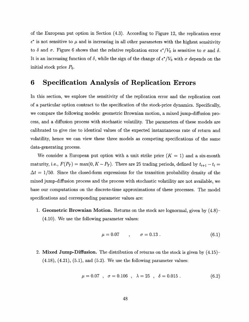
of the European put option in Section (4.3). According to Figure 12, the replication error
c* is not sensitive to gu and is increasing in all other parameters with the highest sensitivity
to and c. Figure 6 shows that the relative replication error e*/V 0 is sensitive to and 6.
It is an increasing function of 6, while the sign of the change of e*/VO with 0c depends on the
initial stock price Po.
6 Specification Analysis of Replication Errors
In this section, we explore the sensitivity of the replication error and the replication cost
of a particular option contract to the specification of the stock-price dynamics. Specifically,
we compare the following models: geometric Brownian motion, a mixed jump-diffusion pro-
cess, and a diffusion process with stochastic volatility. The parameters of these models are
calibrated to give rise to identical values of the expected instantaneous rate of return and
volatility, hence we can view these three models as competing specifications of the same
data-generating process.
We consider a European put option with a unit strike price (K = 1) and a six-month
maturity, i.e., F(PT) = max(0, K - PT). There are 25 trading periods, defined by ti+l - ti =
At = 1/50. Since the closed-form expressions for the transition probability density of the
mixed jump-diffusion process and the process with stochastic volatility are not available, we
base our computations on the discrete-time approximations of these processes. The model
specifications and corresponding parameter values are:
1. Geometric Brownian Motion. Returns on the stock are lognormal, given by (4.8)-
(4.10). We use the following parameter values:
,u = 0.07 , = 0.13 . (6.1)
2. Mixed Jump-Diffusion. The distribution of returns on the stock is given by (4.15)-
(4.18), (4.21), (5.1), and (5.2). We use the following parameter values:
= 0.07 , = 0.106 , A=25 , 6=0.015. (6.2)
48
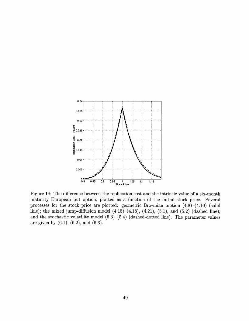
U.U4
0 .0 3 5 ..............................................................
0.03O 0.025
0.015 .. .....
0.01
0.8 0.85 0.9 0.95 1 1.05 1.1 1.15Stock Price
Figure 14: The difference between the replication cost and the intrinsic value of a six-monthmaturity European put option, plotted as a function of the initial stock price. Severalprocesses for the stock price are plotted: geometric Brownian motion (4.8)-(4.10) (solidline); the mixed jump-diffusion model (4.15)-(4.18), (4.21), (5.1), and (5.2) (dashed line);and the stochastic volatility model (5.3)-(5.4) (dashed-dotted line). The parameter valuesare given by (6.1), (6.2), and (6.3).
49
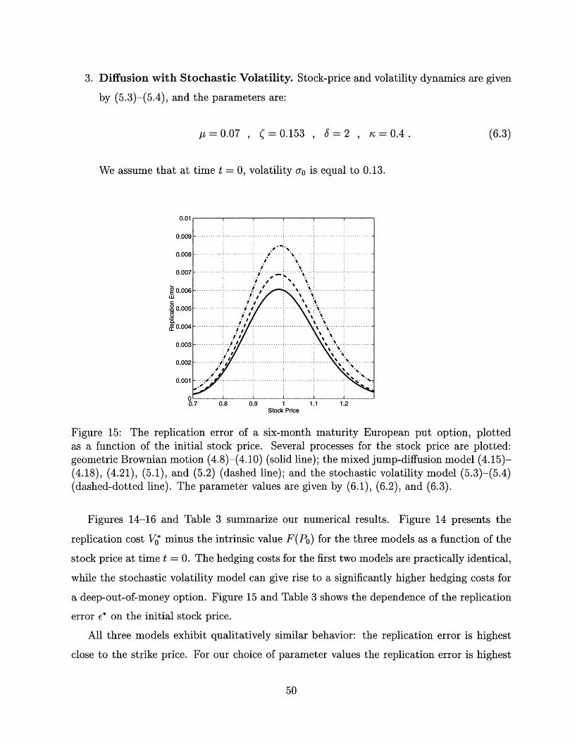
3. Diffusion with Stochastic Volatility. Stock-price and volatility dynamics are given
by (5.3)-(5.4), and the parameters are:
/u=0.07 , (=0.153 , 6=2 , =0.4. (6.3)
We assume that at time t = 0, volatility a0 is equal to 0.13.
0.01
0 .0 0 9 . ..................... ..... .....................
0.008 ... t 8 . s ................: :. \:
: : :0.007 . .. .. ..... .... ............. .
0.003 .. .................... I . ........................0.006 . ......
0.005 ................... i./- .......... .....................(D0.0 : .. \ .
~0.004 ............ C............- . .. .....
* · . .
0.001 .' .4
/'
0.7 0.8 0.9 1Stock Price
1.1 1.2
Figure 15: The replication error of a six-month maturity European put option, plottedas a function of the initial stock price. Several processes for the stock price are plotted:geometric Brownian motion (4.8)-(4.10) (solid line); the mixed jump-diffusion model (4.15)-(4.18), (4.21), (5.1), and (5.2) (dashed line); and the stochastic volatility model (5.3)-(5.4)(dashed-dotted line). The parameter values are given by (6.1), (6.2), and (6.3).
Figures 14-16 and Table 3 summarize our numerical results. Figure 14 presents the
replication cost V0* minus the intrinsic value F(Po) for the three models as a function of the
stock price at time t = 0. The hedging costs for the first two models are practically identical,
while the stochastic volatility model can give rise to a significantly higher hedging costs for
a deep-out-of-money option. Figure 15 and Table 3 shows the dependence of the replication
error e* on the initial stock price.
All three models exhibit qualitatively similar behavior: the replication error is highest
close to the strike price. For our choice of parameter values the replication error is highest
50
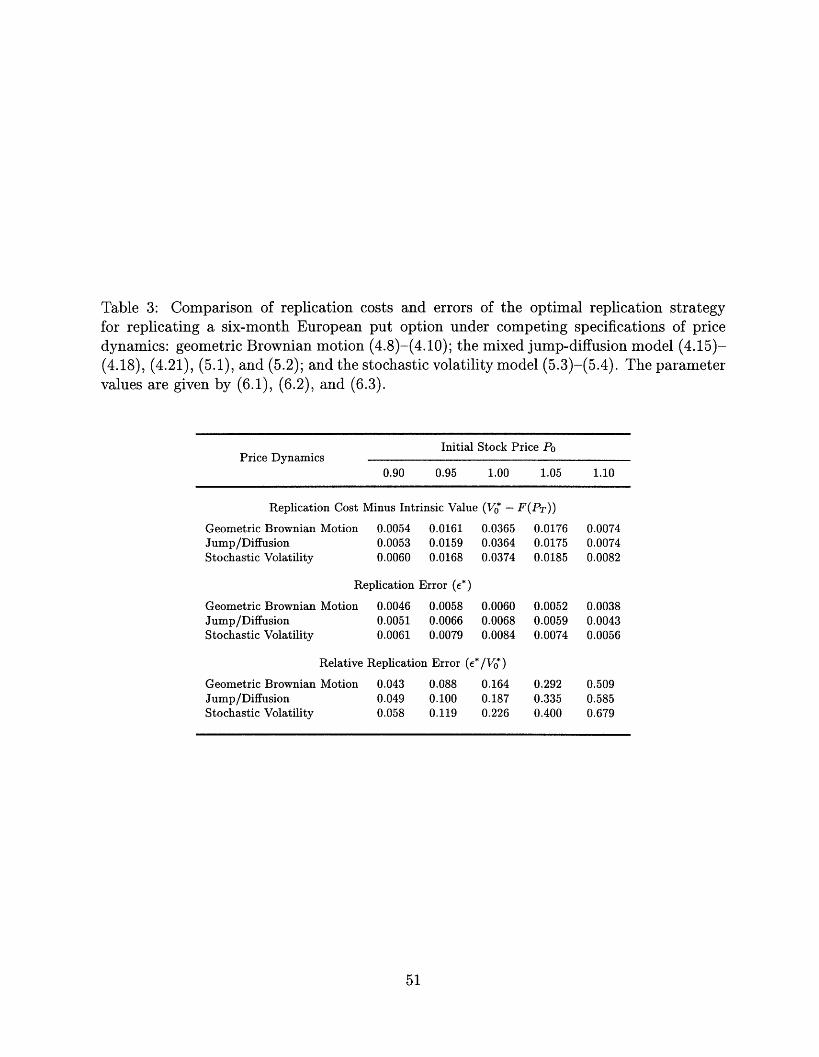
Table 3: Comparison of replication costs and errors of the optimal replication strategyfor replicating a six-month European put option under competing specifications of pricedynamics: geometric Brownian motion (4.8)-(4.10); the mixed jump-diffusion model (4.15)-(4.18), (4.21), (5.1), and (5.2); and the stochastic volatility model (5.3)-(5.4). The parametervalues are given by (6.1), (6.2), and (6.3).
Initial Stock Price P0oPrice Dynamics
0.90 0.95 1.00 1.05 1.10
Replication Cost Minus Intrinsic Value (V* - F(PT))
Geometric Brownian Motion 0.0054 0.0161 0.0365 0.0176 0.0074Jump/Diffusion 0.0053 0.0159 0.0364 0.0175 0.0074Stochastic Volatility 0.0060 0.0168 0.0374 0.0185 0.0082
Replication Error (e*)
Geometric Brownian Motion 0.0046 0.0058 0.0060 0.0052 0.0038Jump/Diffusion 0.0051 0.0066 0.0068 0.0059 0.0043Stochastic Volatility 0.0061 0.0079 0.0084 0.0074 0.0056
Relative Replication Error (e*/V*)
Geometric Brownian Motion 0.043 0.088 0.164 0.292 0.509Jump/Diffusion 0.049 0.100 0.187 0.335 0.585Stochastic Volatility 0.058 0.119 0.226 0.400 0.679
51

for the stochastic volatility model and lowest for geometric Brownian motion. However, this
need not hold in general. As we demonstrate in Section 4.3, the replication error of the
mixed jump-diffusion process depends critically on 6 and A in (4.19, 4.21), thus, by varying
these parameters, one can reverse the order of the curves in Figure 15 without changing the
annualized volatility of the mixed jump-diffusion process.
09
00.7
0 I : m ' X
0 . . . . . ............ ..........................
0.4 ................................ ...... .. ' r...... .
0.2
0, ... ......... i ......... ..
0.8 0.85 0.9 0.95 1 1.05 1.1 1.15Stock Price
Figure 16: The relative replication error of a six-month maturity European put option(relative to the replication cost), plotted as a function of the initial stock price. Severalprocesses for the stock price are plotted: geometric Brownian motion (4.8)-(4.10) (solidline); the mixed jump-diffusion model (4.15)-(4.18), (4.21), (5.1), and (5.2) (dashed line);and the stochastic volatility model (5.3)-(5.4) (dashed-dotted line). The parameter valuesare given by (6.1), (6.2), and (6.3).
The dependence of the relative replication error on the initial stock price is captured
in Figure 16. As in Figure 14, the relative replication error for the first two models are
practically identical, while the stochastic volatility model can exhibit considerably higher
errors. Also, while the relative replication error can be significant, particularly for an out-
of-money option, the variation across the models is not as significant as one would expect.
When continuous-time trading is allowed, the replication error for the geometric Brownian
motion model is zero, while the other two models give rise to strictly positive replication
errors. This is an implication of the fact that the first model describes a dynamically complete
market, while the other two correspond to markets which are dynamically incomplete (due
52

to the absence of a sufficient number of traded instruments).
Nevertheless, as Figure 16 illustrates, the transition from continuous- to discrete-time
trading can smear the differences between these models, leading to relative replication errors
of comparable magnitude. This shows that impossibility of continuous-time trading is just
as important as a source of market incompleteness, as the absence of traded instruments.
7 Conclusion
We have proposed a method for replicating derivative securities in dynamically incomplete
markets. Using stochastic dynamic programming, we construct a self-financing dynamic
portfolio strategy that best approximates an arbitrary payoff function in a mean-squared
sense. When markets are dynamically complete, as in the Black and Scholes (1973) and
Merton (1973) models, our optimal-replication strategy coincides with the delta-hedging
strategies of arbitrage-based models. Moreover, we provide an explicit algorithm for com-
puting such strategies, which can be a formidable challenge in spite of market completeness,
e.g., path-dependent derivatives such as "look-back" options.
When markets are not dynamically complete, as in the case of options on assets with
stochastic volatility or with jump components, our approach yields the minimum production
cost of a self-financing portfolio strategy with a terminal value that comes as close as possible
(in a mean-squared sense) to the option's payoff. This is the essence of the -arbitrage
approach to synthetically replicating a derivative security.
More importantly, we show that if the mean-squared loss function is evaluated with
respect to the equivalent martingale measure, the minimum production cost associated with
the optimal-replication strategy is the equilibrium price of the derivative security. Therefore,
the e-arbitrage approach can also be viewed as a method for pricing, not just replicating,
derivative securities in dynamically incomplete markets. Of course, obtaining the equivalent
martingale measure is the most difficult aspect of asset pricing in incomplete markets, and
we discuss theoretical and empirical approaches to confronting this challenge.
We also argue that the replication error of the optimal-replication strategy can be used
as a quantitative measure for the degree of market incompleteness. Despite the difficulties
in making welfare comparisons between markets with different types of incompleteness (see,
53
for example, Duffie [1987], Duffie and Shafer [1985, 1986], and Hart [1974]), the minimum
replication error of an c-arbitrage strategy does provide one practical metric by which market
completeness can be judged. After all, if it is possible to replicate the payoff of a derivative
security to within some small error E, the market for that security may be considered complete
for all practical purposes even if e is not zero.
Of course, this is only one of many possible measures of market completeness and we make
no claims of generality here. Instead, we hope to have shown that Merton's (1973) seminal
idea of dynamic replication has far broader implications than the dynamically-complete-
markets setting in which it was originally developed. We plan to explore other implications
in future research.
54
A Appendix
The proofs of Theorems 2 and 1 are conceptually straightforward but notationally quite
cumbersome. Therefore, we present only a brief sketch of the proofs below-interested
readers can contact the authors for the more detailed mathematical appendix.
A.1 Proof of Theorem 1
The proof of Theorem 1 follows from dynamic programming. For i = N, (2.14)-(2.16)
are clearly true, given (2.10). We now show that (2.17)-(2.21) describe the solution of the
optimization problem in (2.9). First, as we observed in Section 2.2, the functions ai(., ) are
positive. Together with (2.3) this implies that
EV [I+1 (Vi + Oi(Pi+1 - Pi), Pi+1 , + Vi, Pi, Z]
is a convex function of Oi. Therefore, we can use the first-order condition to solve the
optimization problem in (2.11):
d E [+ (Vi + Oi(P+1 - Pi), Pi+1, Zi+1) Vi, Pi,Z] = 0, (A.1)
where Ji+l(,, ) is given by (2.12). Equation (A.1) is a linear equation in Oi and it is
straightforward to check that its solution, *(i, V,Pi, Zi), is given by (2.13), (2.17), and
(2.18). We now substitute (2.13) into (2.3) and use (2.11) to calculate
Ji(i, Pi, Zi) =
Ev [i+1 (Vi + O*(i, Vi, Pi, Zi) (Pi+1 - Pi),Pi+, Zi+ Vi, Pi, Zi] (A.2)
Equations (2.19)-(2.21) are obtained by rearranging terms in (A.2).
A.2 Proof of Theorem 2
The more tedious algebraic manipulations of this proof were carried out using the symbolic
algebra program Maple. Therefore, we shall outline the main ideas of the proof without
55

reporting all of the details.
The cost-to-go function J(t, Vt, Pt, Zt) satisfies the dynamic programming equation
at + min I 3jZ ii Ot Z toZoa +at Ot 'a 2 azij awL= 3 i,j=O i
1 (Oo-Z 2 J2 (OtoZo)2ow/ a2+ ot E °io jpojZoZi J 0 (A 3)2 a j=o (3)
with boundary condition:
J(T, VT, PT, ZT) = [VT- F(PT, ZT)] 2 (A.4)
where some of the functional dependencies were omitted to simplify the notation.
We must now check that the function J(t, Vt, Pt, Zt), given by (2.26), (2.27)-(2.30), and
the optimal control (2.31), satisfies (A.3)-(A.4). Boundary conditions (2.30) immediately
imply (A.4). Next we substitute (2.26) into (A.3). It is easy to check, using equation
(2.27), that function a(.) is positive. Therefore, the first-order condition is sufficient for the
minimum in (A.3). This condition is a linear equation in t which is solved by (2.31). It is
now straightforward to verify that, whenever functions a(.), b(.), c() satisfy (2.27)-(2.29),
(A.3) is satisfied as well.
56

References
Ait-Sahalia, Y. and A. Lo, 1996, "Nonparametric Estimation of State-Price Densities Im-plicit in Financial Asset Prices", to appear in Journal of Finance.
Aiyagari, R., 1994, "Uninsured Idiosyncratic Risk and Aggregate Saving", Quarterly Jour-nal of Economics 109, 659-684.
Aiyagari, R. and M. Gertler, 1991, "Asset Returns with Transactions Costs and UninsuredIndividual Risk", Journal of Monetary Economics 27, 311-331.
Amin, K., 1993, "Jump Diffusion Option Valuation in Discrete Time", Journal of Finance48, 1833-1863.
Amin, K. and V. Ng, 1993, "Option Valuation With Systematic Stochastic Volatility",Journal of Finance 48, 881-910.
Ball, C. and W. Torous, 1985, "On Jumps in Common Stock Prices and Their Impact onCall Option Pricing", Journal of Finance 40, 155-173.
Banz, R. and M. Miller, 1978, "Prices for State- Contingent Claims: Some Estimates andApplications", Journal of Business 51, 653-672.
Bertsekas, D., 1995, Dynamic Programming and Optimal Control, Vol. I. Belmont, MA:Athena Scientific.
Bick, A., 1995, "Quadratic-Variation-Based Dynamic Strategies", Management Science,41(4), 722-732.
Black, F. and M. Scholes, 1973, "Pricing of Options and Corporate Liabilities", Journal ofPolitical Economy 81, 637-654.
Boyle, P. and D. Emanuel, 1980, "Discretely Adjusted Option Hedges", Journal of FinancialEconomics 8, 259-282.
Breeden, D. 1979, "An Intertemporal Capital Pricing Model with Stochastic InvestmentOpportunities", Journal of Financial Economics 7, 265-296.
Breeden, D. and R. Litzenberger, 1978, "State contingent Prices Implicit in Option Prices",Journal of Business 51, 621-651.
Brennan, M., 1979, "The Pricing of Contingent claims in Discrete-Time Models", Journalof Finance 34, 53-68.
Cox, J. and S. Ross, 1976, "The Valuation of Options for Alternative Stochastic Processes",Journal of Financial Economics 3, 145-166.
Cox, J., J. Ingersoll and S. Ross, 1985, "An Intertemporal General Equilibrium Model ofAsset Prices", Econometrica 53, 363-384.
Derman, E. and I. Kani, 1994, "Riding on the Smile", RISK 7 (February), 32-39.
Duffie, D., 1996, Dynamic Asset Pricing Theory, Second Edition. Princeton, NJ: PrincetonUniversity Press.
57
Duffie, D., 1987, "Stochastic Equilibria with Incomplete Financial Markets", Journal ofEconomic Theory 41, 405-416.
Duffie, D. and C. Huang, 1985, "Implementing Arrow-Debreu Equilibria by ContinuousTrading of Few Long-Lived Securities", Econometrica 53, 1337-1356.
Duffie, D. and M. Jackson, 1990, "Optimal Hedging and Equilibrium in a Dynamic FuturesMarket", Journal of Economic Dynamics and Control 14, 21-33.
Duffie, D. and W. Shafer, 1985, "Equilibrium in Incomplete Markets I: A Basic Model ofGeneric Existence", Journal of Mathematical Economics 14, 285-300.
Duffie, D. and W. Shafer, 1986, "Equilibrium in Incomplete Markets II: Generic Existencein Stochastic Economies", Journal of Mathematical Economics 15, 199-216.
Duffie, D. and M. Richardson, 1991, "Mean-Variance Hedging in Continuous Time", Annalsof Applied Probability 1, 1-15.
Duffie, D. and W. Zam, 1987, "The Consumption-Based Capital Asset Pricing Model",GSB Research Paper #922, Stanford University.
Dybvig, P. and C. Huang, 1988, "Nonnegative Wealth, Absence of Arbitrage, and FeasibleConsumption Plans", Review of Financial Studies 1, 377-401.
Dumas, B., J. Flemming and R.E. Whaley, 1995, "Implied Volatility Functions: EmpiricalTests", working paper, Fuqua School of Business, Duke University.
Dupire, B., 1994, "Pricing with a Smile", RISK 7 (January), 18-20.
Fleming W., R. Rishel, 1975, Deterministic and Stochastic Optimal Control. New York:Springer-Verlag.
F5llmer, H. and D. Sonderman, 1986, "Hedging of Non-Redundant Contingent-Claims", inW. Hildebrand and A. Mas-Colell, eds., Contributions to Mathematical Economics, inHonor of Gerard Debreu. Amsterdam: North-Holland.
Garman, M., 1976, "A General Theory of Asset Valuation under Diffusion State Processes",Working Paper No. 50, University of California Berkeley.
Geske, R., 1979, "The Valuation of Compound Options", Journal of Financial Economics7, 63-81.
Harrison, J. and D. Kreps, 1979, "Martingales and Arbitrage in Multiperiod SecuritiesMarkets", Journal of Economic Theory 20, 381-408.
Hart, O., 1974, "On the Existence of Equilibrium in a Securities Model", Journal of Eco-nomic Theory 9, 293-311.
He, H. and D. Modest, 1995, "Market Frictions and Consumption-Based Asset Pricing",Journal of Political Economy 103, 94-117.
Heaton, J. and D. Lucas, 1992, "The Effects of Incomplete Insurance Markets and TradingCosts in a Consumption-Based Asset Pricing Model", Journal of Economic Dynamicsand Control 16, 601-620.
Heaton, J. and D. Lucas, 1996, "Evaluating the Effects of Incomplete Markets on RiskSharing and Asset Pricing", Journal of Political Economy 104, 443-487.
58
He, H. and N. Pearson, 1991, "Consumption and Portfolio Policies with Incomplete Marketsand Short-Sale Constraints", Journal of Economic Theory 54, 259-304.
Huang, C., 1987, "An Intertemporal General Equilibrium Asset Pricing Model: The Caseof Diffusion Information", Econometrica 55, 117-142.
Hull, J. and A. White, 1987, "The Pricing of Options on Assets With Stochastic Volatili-ties", Journal of Finance 42, 281-300.
Hutchinson, J., Lo., A. and T. Poggio, 1994, "A Nonparametric Approach to the Pricingand Hedging of Derivative Securities Via Learning Networks", Journal of Finance 49,851-889.
Jarrow, R. and A. Rudd, 1982, "Approximate Option Valuation for Arbitrary StochasticProcesses", Journal of Financial Economics 10, 347-369.
Johnson H. and D. Shanno, 1987, "Option Pricing When the Variance is Changing", Journalof Financial and Quantitative Analysis 22, 143-151.
Longstaff, F., 1992, "An Empirical Examination of the Risk-Neutral Valuation Model",working paper, College of Business, Ohio State University, and the Anderson GraduateSchool of Management, UCLA.
Longstaff, F., 1995, "Option Pricing and the Martingale Restriction", Review of FinancialStudies 8, 1091-1124.
Lucas, R., 1978, "Asset Prices in an Exchange Economy", Econometrica 46, 1426-1446.
Lucas, D., 1994, "Asset Pricing With Undiversiable Income Risk and Short Sales Con-straints: Deepening the Equity Premium Puzzle", Journal of Monetary Economics 34,325-341.
Magill, M. and M. Quinzii, 1996, Theory of Incomplete Markets. Cambridge, MA: MITPress.
Merton, R., 1971, "Optimum Consumption and Portfolio Rules in a Continuous-Time Mod-el", Journal of Economic Theory 3, 373-413.
Merton, R., 1973, "An Intertemporal Capital Asset Pricing Model", Econometrica 41, 867-887.
Merton, R., 1976, "Option Pricing when Underlying Stock Returns are Discontinuous",Journal of Financial Economics 3, 125-144.
Merton, R., 1992, Continuous-Time Finance. Cambridge, MA: Blackwell Publishers.
Rady, S., 1994, "State Prices Implicit in Valuation Formulae for Derivative Securities:A Martingale Approach", Discussion Paper No. 181, LSE Financial Markets Group,London, UK.
Rubinstein, M., 1976, "The Valuation of Uncertain Income Streams and the Pricing ofOptions", Bell Journal of Economics 7, 407-425.
Rubinstein, M., 1983, "Displaced Diffusion Option Pricing", Journal of Finance 38, 213-217.
Rubinstein, M., 1994, "Implied Binomial Trees", Journal of Finance 49, 771-818.
59
Schl, M., 1994, "On Quadratic Cost Criteria for Option Hedging" Mathematics of Opera-tions Research 19, 121-131.
Scheinkman, J. and L. Weiss, 1986, "Borrowing Constraints and Aggregate Economic Ac-tivitiy", Econometrica 54, 23-45.
Schweizer, M., 1992, "Mean-Variance Hedging for General Claims", Annals of Applied Prob-ability 2, 171-179.
Schweizer, M., 1995, "Variance-Optimal Hedging in Discrete Time", Mathematics of Oper-ations Research 20, 1-31.
Shimko, D., 1993, "Bounds of Probability", RISK 6, 33-37.
Stroud, A., 1971, Approximate Calculation of Multiple Integrals. Englewood Cliffs, NJ:Prentice-Hall.
Stutzer, M., 1995, "A Simple Nonparametric Approach to Derivative Security Valuation",forthcoming in the Journal of Finance.
Telmer, C., 1993, "Asset-Pricing Puzzles and Incomplete Markets", Journal of Finance 48,1803-1832.
Toft, K., 1996, "On the Mean-Variance Tradeoff in Option Replication with TransactionsCosts", Journal of Financial and Quantitative Analysis 31, 233-263.
Weil, P., 1992, "Equilibrium Asset Prices with Undiversifiable Labor Income Risk", Journalof Economic Dynamics and Control 16, 769-790.
Wiggins, J., 1987, "Option Values Under Stochastic Volatility: Theory and Empirical Es-timates", Journal of Financial Economics 5, 351-372.
60