prices and quantities of electricity in the u.s ...econ-server.umd.edu/~haltiwan/pqem.pdfpreliminary...

PRELIMINARY DRAFT

Prices and Quantities of Electricity in the U.S. Manufacturing Sector: A Plant-Level Database and Public-Release Statistics, 1963-2000

By Steven J. Davis, Cheryl Grim, John Haltiwanger and Mary Streitwieser*

November 9, 2007

Abstract

This paper describes the Prices and Quantities of Electricity in Manufacturing

(PQEM) database, which contains plant-level observations on electricity purchases, electricity prices and electricity suppliers for the U.S. manufacturing sector. To construct the database, we link plant-level data on electricity prices and quantities in the Annual Survey of Manufactures (ASM) to information on electricity suppliers from the Energy Information Administration and other sources. The resulting database contains about 1.8 million annual observations over the period from 1963 to 2000. *University of Chicago, NBER and American Enterprise Institute; Bureau of the Census; University of Maryland, Bureau of the Census and NBER; and Bureau of Economic Analysis, respectively. The analysis and results presented in this paper are attributable to the authors and do not necessarily reflect concurrence by the Center for Economic Studies at the U.S. Bureau of the Census. This work is unofficial and thus has not undergone the review accorded to official Census Bureau publications. The views expressed in the paper are those of the authors and not necessarily those of the U.S. Census Bureau. All results were reviewed to ensure confidentiality. The views expressed in this paper are solely those of the authors and not necessarily those of the U.S. Bureau of Economic Analysis or the U.S. Department of Commerce. We thank Monica Garcia-Perez for excellent research assistance and colleagues at the Center for Economic Studies for many helpful comments. We are especially grateful to Rodney Dunn for comments and assistance with the EIA 861 data files. Davis and Haltiwanger gratefully acknowledge research support from the U.S. National Science Foundation under grant number SBR-9730667.

1

1. Introduction This paper describes the Prices and Quantities of Electricity in Manufacturing

(PQEM) database, which contains plant-level observations on electricity purchases,

electricity prices and electricity suppliers for the U.S. manufacturing sector. To construct

the database, we link plant-level data on electricity prices and quantities in the Annual

Survey of Manufactures (ASM) to information on electricity suppliers from the Energy

Information Administration and other sources. The resulting database contains about 1.8

million annual observations over the period from 1963 to 2000. Table 1 summarizes the

scope and coverage of the PQEM.

In constructing the PQEM, we devote considerable effort to treating anomalous

data on electricity prices and quantities in the ASM. We identify a number of coding

errors in the ASM data, and we find that the raw ASM data contain high error rates in

1983 and from 1989 to 1991. As explained below, we develop procedures to correct or

impute values for the mismeasured data, paying special attention to the years with high

error rates. We also address several other measurement issues pertaining to ASM sample

weights in 1963 and 1967, erroneous geographic indicators, and the creation of consistent

industry and geography codes over time.

To match manufacturing plants in the ASM to their electricity suppliers, we

proceed as follows. First, we draw upon news articles and other public sources to compile

a list of manufacturing plants that purchase electricity directly from one of the six largest

public power authorities in the United States. Second, we rely on the Annual Electric

Power Industry Report to identify the set of electric utilities that serve each county in the

2

United States.1 Third, among the utilities that supply electricity to a given county, we use

the Annual Report to determine which one accounts for the largest share of electricity

sales to industrial customers in the same state. We designate this utility as the best-match

utility serving industrial customers in that county. Fourth, we assign that best-match

utility to all manufacturing plants located in the county unless specific information to the

contrary appears in our list of direct purchasers from public power authorities. By

construction, no best-match utility operates in more than one state. We adopt this

approach because of the important role played by state authorities in electric utility

regulation and electricity pricing. Among the 733 distinct best-match utilities in the

PQEM, 13 are accounted for by the 6 public power authorities.

Our procedure for assigning electricity suppliers to manufacturing plants is

imperfect – only 460 of the 3,031 counties covered by the PQEM are supplied by a single

electric utility.2 To address this issue, we refine our matching procedures by drawing on

more detailed information on utility service areas for selected states. This procedure is

described in more detail in Section 2.4 and Technical Appendix A. Despite the remaining

potential for assignment errors, our procedure has proved useful for the study of spatial

variation in electricity prices and for the study of differences among utilities in pricing

schedules.

The plant-level data in the PQEM can be usefully grouped by state, county,

industry, plant size, electricity price, electricity purchases, electricity supplier and other

1 To the best of our knowledge, such data are unavailable prior to 1999, so we apply the data for 2000 to all years covered by the PQEM. 2 This number excludes electric utilities with zero statewide industrial revenue. In the PQEM, 459 counties are served by a single utility, 776 are served by 2 utilities, 791 are served by 3 utilities, 536 are served by 4 utilities, 440 are served by 5-7 utilities, and the remaining 29 counties are served by 8-12 utilities.

3

classification variables. We exploit these classification variables to produce a large

number and variety of electricity price and quantity statistics for public release. Table 2

summarizes the contents of the PQEM public-release statistics, which will be made

available for download at a future date.

Tables 3 and 4 report selected summary statistics on electricity prices and

quantities for manufacturing plants and best-match utilities. Not surprisingly, Table 3

shows tremendous heterogeneity among manufacturing plants in the quantity of

purchased electricity. Of perhaps greater interest, Table 3 also reveals large differences in

electricity prices among manufacturing plants. For example, the price paid by

manufacturing plants in 1963 ranges from 3.45 cents per KWh at the 10th centile of the

shipments-weighted distribution to 8.82 cents at the 90th centile. Similarly, Table 4 shows

considerable variation among utilities in average electricity prices. Figure 1 highlights

large changes over time in the dispersion of electricity prices among manufacturing

plants, a phenomenon that we study in some detail in Davis et al. (2007). Figure 2 shows

annual averages of electricity cost’s percentages variable costs, intermediate input costs,

and electricity costs.3

The paper proceeds as follows. Section 2 briefly describes the data sources for the

PQEM, and Section 3 describes the creation of industry codes in the PQEM. Section 4

describes the identification of ASM plants in the 1967 Census of Manufactures (CM) and

the creation of ASM sample weights for 1963 and 1967. Section 5 describes the

geography codes in the PQEM. Section 6 discusses the construction of electricity

3 Variable costs are defined as CP (cost of materials and parts) + CR (cost of resales) + CW (cost of contract work) + EE (electricity expenditures) + CF (cost of fuels) + SW (salaries and wages). Intermediate input costs are defined as CP + CW + EE + CF. Energy costs are defined as EE + CF.

4

purchase level variables. Sections 7 and 8 explain the imputations we used for

observations with clearly unreasonable electricity prices. Section 9 discusses the handling

of total value of shipments outliers in the PQEM. In Section 10, we describe the

distribution of annual plant electricity purchases by utility ownership type.

2. Sources for the PQEM Database

2.1 The Annual Survey of Manufactures

The ASM is a large sample of manufacturing plants with five or more employees.

Larger plants are sampled with certainty, and sampling probabilities for other plants vary

inversely with plant size. The ASM gathers data on roughly 60,000 plants per year, which

jointly account for about three-quarters of employment in the manufacturing sector. ASM

data are available in electronic form from 1973, and similar data are available from the

CM in 1963 and 1967.4 See the appendix to Davis, Haltiwanger and Schuh (1996) for a

detailed discussion of ASM coverage and sampling procedures.

2.2 The Annual Electric Power Industry Report

The Energy Information Administration collects data from participants in the

electric power industry through its EIA 861 form, also known as the Annual Electrical

Power Industry Report. Electric utilities, wholesale power marketers, energy service

providers and electric power producers are required by law to complete the EIA 861

form. The Annual Report includes data on revenues from electricity sales to industrial

4 The ASM and Census files that we use to construct the PQEM are the versions maintained in the Center for Economic Studies Data Warehouse as of March 2005. The Center for Economic Studies is part of the U.S. Census Bureau. Plant-level data in the ASM, Census and PQEM can only be accessed at the Center and the several U.S. Census Bureau Research Data Centers located in the United States. Information on the process for accessing the plant-level data is available at http://www.ces.census.gov/.

5

customers by state for each utility and a list of the counties served by the utility.5 It also

specifies whether a utility is an investor-owned, public or cooperative enterprise.6

Electronic versions of the Annual Report are available from the Energy Information

Administration at www.eia.doe.gov/cneaf/electricity/page/eia861.html.

2.3 Direct Purchasers from Public Power Authorities

Manufacturers that purchase directly from public power authorities typically

consume large quantities of electricity, often operate their own transformers, and often

obtain electrical power at lower prices than other plants. These direct purchasers are few

in number, but they account for a large fraction of electricity purchases in some counties,

and they constitute a distinct demand-side segment of the retail electricity market. For

these reasons, we sought to separately identify direct purchasers. Unfortunately, the EIA

861 data file does not contain county coverage information for all public power

authorities, nor does it contain other information that identifies direct purchasers.

To address this issue, we draw on a variety of public sources that specifically

identify direct purchasers from the four public power authorities with the largest

industrial revenues in 2000: the Tennessee Valley Authority (TVA), the Bonneville

Power Administration (BPA), Santee Cooper (SC), and the New York Power Authority

(NYPA). Additionally, we identify direct purchasers from the Grand River Dam

5 The Annual Report also reports the North American Reliability Council (NERC) regions in which a utility operates. NERC regions do not necessarily follow county or state boundaries. See pages 6-7 of EIA (1998) for more information on NERC regions. 6 The eight ownership categories in the EIA 861 data file are: private, power marketer, cooperative, federal, municipal, sub-division, municipal marketer, and state. The EIA 861 survey respondent provided this ownership information. Note that utilities with power marketer and municipal marketer ownership categories do not appear in the PQEM because these types of utilities do not sell power directly to end-use customers.

6

Authority (GRDA) and the Colorado River Commission of Nevada (CRC).7 In 2000,

these six public power authorities account for nearly 98% of all public power authority

industrial revenue and 3% of all utility revenue from industrial customers (source: 2000

EIA 861 files). We identify an average of 84 plants per year that are direct serve

customers of one of our six major public power authorities.8 Pooling across years in the

PQEM, the direct-serve customers of our six major public power authorities account for

3.6% of all electricity purchases (on a shipments-weighted basis). The shipments-

weighted mean of electricity purchases for direct-serve customers of our six public power

authorities is 1,030.58 GWh.

2.4 Electric Utility Customers

We link plants that are not direct serve customers of public power authorities to

their electric utilities using the 2000 EIA 861 file. We rely on the EIA 861 file to identify

the set of electric utilities that serve each county in the United States. First, we use the

EIA 861 file to determine which electric utility accounts for the largest share of

electricity sales to industrial customers in the same state. We designate this utility as the

best-match utility serving industrial customers in that county. By construction, no best-

match utility operates in more than one state.

7 Specifically, we use public information to identify large aluminum smelting plants in the Pacific Northwest as direct purchasers from the BPA. For TVA, because it has a huge service area, we concentrate on certain industries (Aluminum, Steel, Other Primary Metals, Chemicals, Paper and Forest, Motor Vehicles and Motor Equipment) when searching for direct serve customers. We do not focus on specific industries when identifying direct-serve industrial customers for the other public power authorities. For CRC and NYPA, we found publicly available lists of direct-serve power customers. A detailed technical note with a full description of our sources and methods for identifying direct purchasers is available to researchers who have permission to access the PQEM micro data at a Census Research Data Center. 8 The number of plants identified as public power authority customer plants ranges between 58 and 94 plants per year.

7

As discussed earlier, the procedure described above for assigning electricity

suppliers to manufacturing plants is imperfect because many counties are served by

multiple electric utilities. To address this issue, we refine our matching procedures by

drawing on detailed information on utility service territories. First, we incorporate

information from GIS maps of electric utility service areas for six states: Kansas,

Kentucky, Maine, Minnesota, Ohio and Wisconsin.9 We use address information from

the Business Register (BR) to assign latitude and longitude to as many plants as possible

and then overlay the GIS service area map to determine the electric utility that serves the

plant. We also incorporate information from a zip code-utility concordance for three

additional states, California, New York and Rhode Island. We use address information

from the 2000 BR to assign zip code to as many plants as possible and then use the zip

code list to determine the electric utility that serves the plant. We then use a nearest

neighbor matching procedure to assign electric utilities based on the zip code information

for plants that do not appear in the year 2000. Finally, we use printed maps of electric

utility service areas and county boundaries to refine our utility assignments for Florida,

Illinois, Louisiana, Maryland, Michigan, Missouri, Pennsylvania, South Dakota and

Wyoming. We examine each county visually, and if one utility clearly covers most of the

county, we assign that utility to all plants in the county. If the county is not covered

primarily by a single utility, we retain our original county-based utility match. See

Technical Appendix A for more information on our utility assignments.

Introduction of the GIS and zip code data allows us to calculate an overall

estimated match accuracy rate for the PQEM. Let Z denote the set of plants with GIS

9 We obtained the Minnesota GIS map from the Minnesota Department of Commerce. This map is an intermediate and unofficial version.

8

and/or zip code information on utility service territories, and let ^Z be the complement;

i.e., all other plants. Let ( )n ⋅ be a function that returns the number of utilities serving

industrial customers in the county according to the EIA 861 files. Lump all counties

served by five or more utilities into a single category, called “5+”. Define ( )N i as the

number of ASM-sampled plants for which ( )n e i= for 1,2,3,4,5 .i = + Define ( ; )N i Z

and ( ;^ )N i Z as analogous quantities for Z and ^Z. For present purposes, treat customers

that purchase directly from public power authorities as belonging to a county served by a

single utility.

First, for plants in Z, we construct the share of plants that are accurately matched

by county-level matching in counties served by i utilities as shown in (1).

[ ] 1

{ : ( ) }

( ) ( ; ) ( ) for 1, 2,3, 4,5 .e Z n e i

p i N i Z I e i−

∈ =

= = +∑ (1)

where ( )I ⋅ is an indicator function that returns a value of one if our county-based

matching algorithm produces a correct match, and zero otherwise. We calculate these

probabilities in a completely unweighted manner (no use of ASM sampling weights). By

construction, (1) 1.p =

Information on service territories by zip code is not always sufficient to determine

an exact match. As a lower bound on the probability that our county-based algorithm

assigns the correct utility in these cases, we compute the following scaled probabilities:

( )[ ] ( ) ( )( ){ }∑

=∈

−=ienZe

LB ezeIZiNiq:

1 /~;)( for i = 1, 2, 3, 4, 5+ (2)

9

where ( )z e is the number of utilities that serve the zip code in which e is located. In

words, ( )LBiq is the fraction of ASM-sampled plants in counties served by i utilities that

cannot be uniquely matched using zip code matching, scaled down by the number of

utilities that serve e’s zip code. By construction, ( ) 01 =LBq . The q’s are constructed in a

completely unweighted manner.

In practice, our algorithm is more accurate than random assignment, because we

exploit additional information on utility revenues at the state level. Hence, we use the

( )I ⋅% function in (1) to provide a better estimate for the probability of an accurate match

when plant e’s zip code is served by multiple utilities:

( )[ ] ( ) ( )( ){ }∑

=∈

−=ienZe

ezpeIZiNiq:

1 )(~;)( for i = 1, 2, 3, 4, 5+ (3)

It is worth remarking that the expression for q(i) in (3) is also likely to underestimate the

probability of an accurate match, because the p(i) function in (1) reflects only the fraction

of plants that are correctly matched with certainty.

We can now estimate a lower bound on the overall rate of an accurate match as

( ) ( ) ( )[ ] ( ) ( )

+

+= ∑∑ ∑

∈

+

= ∈ Zei ZELBLB ezesiqipesA /ˆ

5

1 ^ (4)

where the plant-level weights s(e) satisfy ( ) 1.e

s e =∑ We estimate the overall rate of an

accurate match as shown in (5).

( ) ( ) ( )[ ] ( ) ( )( )

+

+= ∑∑ ∑

∈

+

= ∈ Zei ZEezpesiqipesA

5

1 ^

ˆ (5)

10

The first term on the right side of (5) captures states with county-level matching, and the

second term captures states with GIS/zip code matching. The estimated match accuracy

rates in equations (4) and (5) do not capture the impact of the nearest neighbor zip

corrections or the hand corrections to the county-level utility assignments that we made

by using printed maps of utility service territories. In this respect, the match accuracy

estimates in (4) and (5) are understated. As remarked above, we exploited printed maps

of utility service territories for nine states. Table 5 shows average annual utility match

statistics for the PQEM database. The sample-weighted average annual estimated rate of

an accurate match is 64 percent. We assume all nearest neighbor zip assignments are

correct with p(i) = 1 for all i to get an upper bound for the effect of including nearest

neighbor zip assignments in the estimated rate of an accurate match. This yields an upper

bound average annual estimated rate of an accurate match of 77 percent.

2.5 State-Level Data on Power Sources for Generated Electricity

The Energy Information Administration makes annual state-level data on fuels

and other sources of power for the generation of electricity available to the public. These

data are available in the State Energy Data System (SEDS) for all 50 states and the

District of Columbia from 1960 to 2000.

We use the SEDS data to create annual state-level shares of fuels used for

electricity generation for the following five categories: coal, petroleum and natural gas,

hydropower, nuclear power, and other (includes geothermal, wind, wood and waste,

photovoltaic, and solar).10 Figure 3 shows the annual national fuel shares of electricity

10 We use the SEDS updated through 2000. Current SEDS data is available at http://www.eia.doe.gov/emeu/states/_seds.html. A detailed technical note on the creation of fuel shares from the EIA SEDS data is available from the authors upon request.

11

generation calculated from the SEDS data. Coal is used to generate more electricity than

any other fuel in every year from 1960 to 2000. Also note, “other” fuels account for very

little electricity generation throughout the entire period.

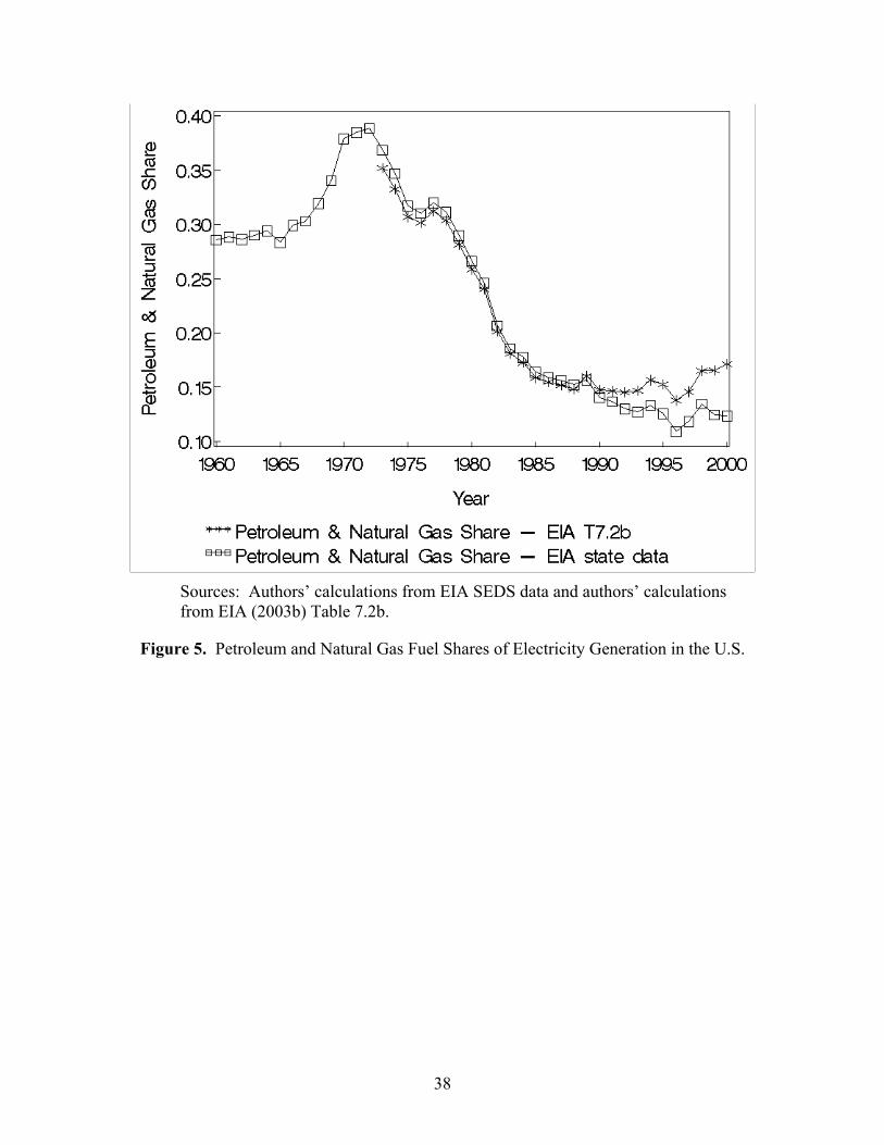
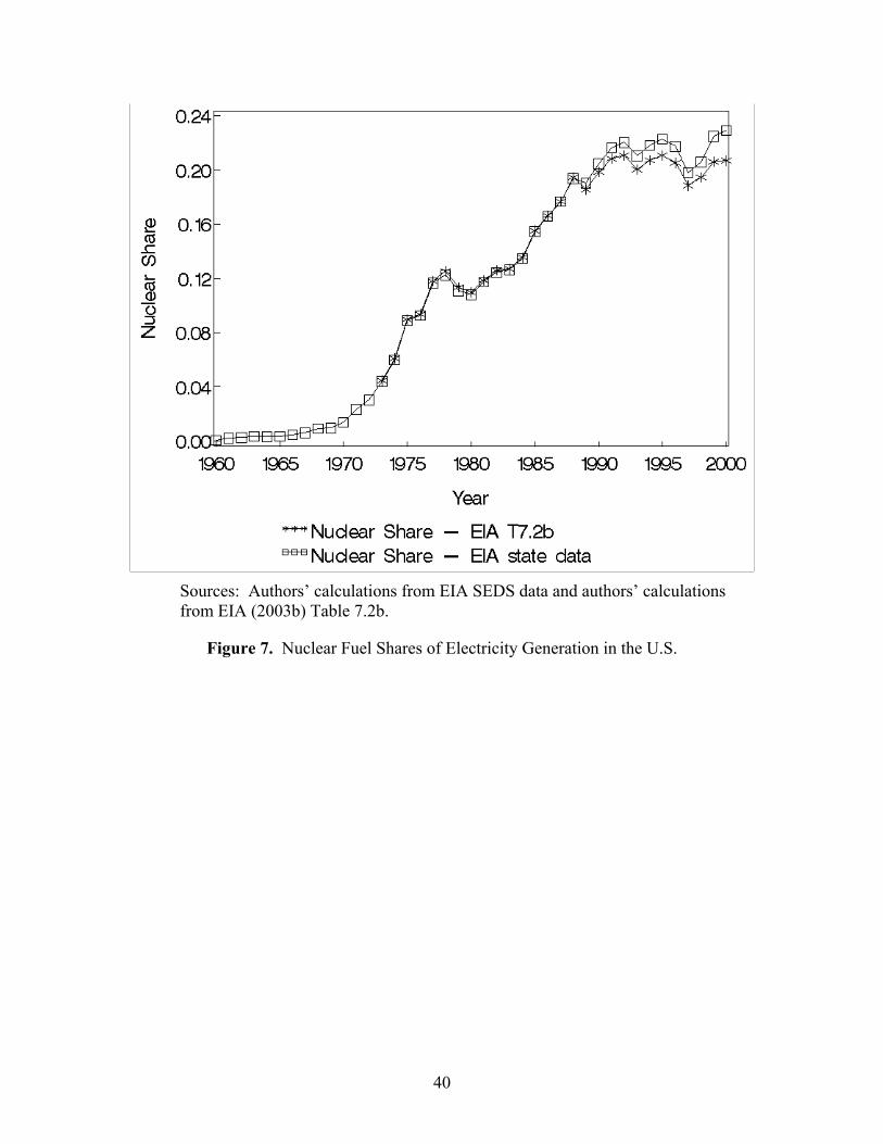
Figures 4 - 8 show comparisons of national fuel shares for electricity generation

calculated from SEDS data and fuel shares calculated from Table 7.2b of EIA (2003c).11

The fuel shares we calculate from SEDS data follow the pattern of and are close in

magnitude to the EIA Table 7.2b data for all fuels except “other”. Also of note, the gap

between the SEDS-based data and the EIA Table 7.2b data gets larger in 1989 because

the SEDS data does not contain non-utility generation for any fuels other than

hydropower. There is a particularly large difference for “other” fuels because power

generated by wind, geothermal, and other sources is, in large part, generated by non-

utilities. However, since the “other” category is such a small percentage of electricity

generation, we do not address this difference.

3. Industry Codes

The PQEM contains a revised industry variable, newind. The industry codes in the

variable newind are 4-digit SIC industries. We use a combination of 1972 and 1987 SIC

codes across years. Years prior to 1987 are coded with 1972 SIC codes, and years 1987

and later are coded with 1987 SIC codes.12 Overall, the PQEM contains 447 1972 SIC

codes and 458 1987 SIC codes.

11 Table 7.2b can be found in EIA (2003c). Note the fuel shares shown in Figures 4.4 - 4.8 are calculated simply by adding up kWh generated by the fuels in each of the five categories and dividing by “total” kWh generated. 12 This does not cause problems for analysis as long as all analyses involving the newind variable are either done by year or for groups of years that do not straddle 1987.

12

We want researchers to have the option of using the NBER-CES producer price

indices in conjunction with the PQEM.13 Therefore, any industries that cannot be

matched to the NBER-CES producer price index database are considered invalid.14 If

possible, corrections are made to invalid industry codes using data from surrounding

years. Observations for which corrections cannot be made are dropped. As can usually be

expected with microdata, there are some complexities involved in creating the newind

variable from the existing ASM industry variables. Technical Appendix B contains a

detailed description of how we create the newind variable.

4. Identification of ASM Plants in CM Years and Sample Weights

The ET (establishment type) variable is used to identify ASM plants in all years

except for 1967. ET = 0 indicates that the plant is an ASM plant. Unfortunately, there is

no simple way to identify ASM plants in the 1967 CM. The variable ET is equal to one

for all observations on the 1967 CM file. We combined information on certainty cases

from the 1967 CM publication and information on typical imputation patterns for non-

ASM plants to identify ASM plants in the 1967 CM. Technical Appendix C describes our

methodology for identifying ASM plants in the 1967 CM in detail.

As discussed in Section 2.1, the ASM is a sub-sample of the universe of

manufacturing plants. Hence, sample weights are required to create nationally

representative statistics. Generally, ASM sample weights are available on the ASM and

CM microdata files in the variable WT. However, ASM sample weights are not available

13 The NBER-CES producer price indices are available at http://www.nber.org/nberces/nbprod96.htm. There is a price index value for each year and 4-digit SIC code. 14 We drop 2794, which is in the 1972 NBER-CES database. Industry 2794 is listed as a discontinuous industry in Davis, Haltiwanger, and Schuh (1996) and is put into 2793. We drop 2067 (Chewing Gum) as a valid industry in the 1987 codes. For confidentiality reasons, Census combined 2067 into 2064 (Candy and Other Confectionary Products). We do this as well during the creation of the PQEM.

13

on the 1963 and 1967 CM plant-level data files. Technical Appendix D describes the

method we use to estimate ASM sample weights for the 1963 and 1967 CM surveys.

5. Geography Codes

The PQEM contains a time consistent Federal Information Processing Standards

(FIPS) combined county-state identifier, cyfstn.15 Unfortunately, there are problems with

the FIPS county and state code identifiers on some of the ASM and CM microdata files.

Further, FIPS county codes have changed over time. Technical Appendix E describes

changes we make to the state and county FIPS codes to make them correct and consistent

across time in the PQEM.

6. Creation of Purchase Level Variables

In addition to log purchased electricity itself, we create four variables to measure

the electricity purchase levels of plants by where they fit into the distribution of

purchased electricity. First, we compute two unweighted decile and centile purchase level

variables to use in our imputation procedures. Then we compute shipments-weighted

decile and centile purchase level variables for use in our analysis.

We compute the unweighted distribution of log purchased electricity across all

plants by year. Then we compute deciles of purchased electricity and assign each plant-

year observation a value in the variable, decile_uu, based on where it fit into the

distribution. A value of decile_uu equal to one implies that the plant’s quantity of

purchased electricity for that year falls in the lowest decile of users for that year.

Additionally, we create a variable, centile_uu, representing the unweighted electricity

15 The National Institute of Standards and Technology (NIST) issues FIPS codes. NIST publications related to FIPS codes can be found at http://www.itl.nist.gov/fipspubs/.

14

purchase level centile of the plant in that year. We create this variable by ordering plants

from lowest to highest quantity of purchased electricity and dividing them into 100

equally sized groups.16 A value of centile_uu equal to one implies that the plant’s

quantity of purchased electricity for that year falls into the group containing the smallest

electricity purchasers in that year.

Further, we create two measures of where a plant fits in the shipments-weighted

distribution of electricity purchases. For one measure, we pooled observations over all

plants within a year and computed shipment-weighted deciles of the resulting distribution

of electricity purchases. We then assigned each plant-year observation a decile rank from

1 to 10 based on where it fits in the pooled distribution for that year and called this

variable decile. For a second shipments-weighted measure, we assigned centile ranks

from 1 to 100 in the same manner to the variable centile.

7. Imputations for Observations with Unreasonable Electricity Prices

This section describes our procedures for identifying and imputing values for

electricity variables for observations with unreasonable electricity prices, purchases,

and/or expenditures. We impute values for the following two electricity variables: EE =

electricity expenditures and PE = quantity of purchased electricity. Annual electricity

prices are calculated as EE divided by PE.

We employ two data filters to identify observations with unreasonable values of

the electricity variables. The first data filter identifies observations with specific problems

with the electricity variables. We apply an imputation algorithm to the observations

16 We also created a centile variable based on percentiles of the distribution by year. The results were very similar. The use of equally sized groups allows us to avoid potential disclosure problems.

15

identified as problem observations by the first data filter. Following this, we apply a

second, more general, data filter to the electricity variables to identify remaining problem

observations. We use the same imputation algorithm to correct as many of these problem

observations as possible.

Data Filter 1: Specific Problems

Data Filter 1 marks observations with any of the following characteristics as

problem observations.

• The observation has a real price of electricity ≥ $0.30 per kWh.17

• The observation has a nominal price of electricity equal to exactly $0.001 per

kWh.

• The observation has missing or zero PE and/or EE.

There is a major data anomaly in the 1983 ASM. The variables EE and PE are

equal for many plants. Although this phenomenon occurs across all purchase deciles, it

occurs primarily with plants that are smaller, where size is defined in terms of their

amount of purchased electricity. Ninety percent of all EE = PE observations occur in the

three smallest plant unweighted purchase deciles, representing eight percent of all small

plants.18 Nearly 1,500 plants (3 percent of all ASM plants in 1983) have a nominal price

of electricity equal to $1 per kWh (i.e., EE = PE for that plant) in 1983. Other years have

17 Nominal prices were deflated to real 1996 prices using the annual implicit GDP deflator from the Bureau of Economic Analysis. 18 We created unweighted purchase deciles for use in our imputation process. Here, “purchase decile” refers to the decile class (in terms of the amount of purchased electricity) of the plant. Purchase deciles are created by year based on the unweighted distribution of log PE for 1963, 1967, and 1972-2000. The variable decile = 1 represents the decile of the smallest electricity purchasers.

16

only a trivial number of occurrences: less than 0.2 percent.19 Further, 1983 contains a

relatively large number of plants with real price of electricity greater than 30 1996 cents

per kWh. According to EIA data, these prices are very high; average industrial electricity

prices were $0.0485 per kWh in 1983.20

For the purpose of examining and correcting the log price of electricity in this

technical report, we consider all plants with a real price of electricity ≥ $0.30 per kWh to

be “problem” plants. We feel this is a reasonable cutoff for problem plants for a couple of

reasons. First, this cutoff is six times the highest average U.S. industrial electricity price

as reported by the EIA. Second, a quick look at the Manufacturing Energy Consumption

Survey (MECS) plant-level data for 1988, 1991, 1994 and 1998 shows that less than one

fifth of one percent of the plants have real electricity prices ≥ $0.30 per kWh.

There are over 2,900 plants in 1983 with real electricity price ≥ $0.30 per kWh.

This is close to 6 percent of all plants in the 1983 ASM sample. While this may not seem

like a large percentage, you can see in Figure 9 that a small percentage of plants can have

a big effect on important characteristics of the data, such as the standard deviation.

Specifically, Figure 9 shows the completely unweighted standard deviation of the log

price of electricity from the 1963, 1967 and 1972-2000 ASM. It is easy to see that the

standard deviation of the log price of electricity in 1983 is disproportionately high

relative to surrounding years. Additionally, problem observations with a real price of

electricity≥ $0.30 per kWh are not uniformly distributed among levels of energy users.

Approximately 15 percent of plants in the three smallest plant purchase deciles have a

19 There are observations for which the price of electricity is missing. These are observations for which PE and/or EE are zero or missing so the price of electricity could not be calculated. 20 This information can be found on the EIA Internet site: http://www.eia.doe.gov.

17

real price of electricity≥ $0.30 per kWh in 1983. Thus, failure to correct for problems

with the EE and PE variables could lead to especially poor results for plants that purchase

relatively smaller amounts of electricity.

Further, there are close to 40 observations among all years with nominal price of

electricity equal to exactly $0.001 per kWh. Looking at the data shows that PE is simply

EE multiplied by 1000. Since this is quite unlikely to be true, these observations will also

be considered “problem” observations. Finally, all observations with missing or zero PE

and/or EE will be considered “problem” observations.

Data Filter 2: General Outliers

After we create “corrected” log price of electricity values for as many as possible

of the problem observations identified by Data Filter 1, we apply a second data filter to

catch general outliers. An observation is a general outlier according to Data Filter 2 if

either of the following are true.

• The log price of electricity is both a time series and cross-sectional outlier within

its’ best-match utility area and state.21

• PE in year t is greater than or equal to the 75th percentile of PE for year t and PE

in year t is at least 10 times greater than PE in year t-1 and PE in year t is at least

10 times greater than PE in year t+1.22

An observation in year t is a time series outlier if the difference between the log price of

electricity in year t-1 and the log price of electricity in year t is more than 0.5 and the

difference between the log price of electricity in year t+1 and the log price of electricity

21 The best-match utility area of the plant is based on EIA data that is merged to the ASM data by county. 22 This condition on PE is required in addition to the condition on the log price of electricity because if both PE and EE are outliers for the plant, the electricity price may still be reasonable.

18

in year t is more than 0.5. An observation in year t is a cross-sectional outlier within its’

best-match utility area and state if the difference between the observation’s log price of

electricity and the mean log price of electricity for its’ best-match utility area and state is

greater than 1.

Imputation Algorithm

We split our imputation algorithm into two parts. First, we correct the log price of

electricity. Once we have corrected the log price of electricity, we correct the values of

EE and PE. The algorithm to correct the log price of electricity is shown below.

(1) Estimate decile-county log nominal price of electricity (lpe) changes using non-

problem observations. Apply this price change to the non-problem previous (or

subsequent) year log price of electricity to calculate a corrected log price of

electricity.

(2) If step 1 does not provide a corrected log price of electricity, estimate county log

price of electricity changes using non-problem observations. Apply this price change

to the non-problem previous (or subsequent) year log price of electricity to calculate a

corrected log price of electricity.

(3) If steps 1 and 2 do not provide a corrected log price of electricity, run the following

regression by year on non-problem observations:

lpeet = α0 + α1TEet + α2COUNTYet (6)

where lpe = log price of electricity, TE = total employment, COUNTY = county where

the plant is located, e = plant and t = YEAR. Use the predicted lpe from regression (6)

19

as the corrected log price of electricity for all remaining problem observations in that

county for that year.

We first identify problem observations with Data Filter 1 and create corrected log

price of electricity values (lpe_corrected) using the algorithm above. Using the corrected

observations, we then identify additional problem observations with Data Filter 2 and

create corrected log price of electricity values using the algorithm above. Finally, we

calculate corrected PE and EE values as follows.

(1) If EE is non-zero and non-missing, calculate corrected PE as

PE_corrected = EE / lpe_corrected.

(2) If EE is zero or missing, but PE is non-zero and non-missing, calculate corrected

EE as EE_corrected = PE * lpe_corrected.

(3) If both EE and PE are missing or zero, but lpe was corrected using either the

previous or subsequent year data, assign corrected PE as the value of the current

year mean of the unweighted purchase centile (centile_uu) of the previous or

subsequent year that was used to correct lpe. 23 Then calculate corrected EE as

EE_corrected = PE * lpe_corrected. Note that observations with both PE and EE

equal to zero or missing and no non-problem previous or subsequent year

observations cannot have PE and EE corrected though they might have a

corrected lpe.

Results of Imputation

Figure 10 shows the unweighted standard deviation of the log price of electricity

after the correction algorithm has been applied to all years. We no longer see the huge 23 The centile_uu variable is calculated as described in Section 7.

20

peak in the standard deviation in 1983 that we saw in Figure 9. The total number of

“problem” observations in 1983 is close to 6,000. Of these, nearly half were fixed using

Step 1 of our log price of electricity correction algorithm with the previous year. In total,

we were able to fix approximately two-thirds of the problem observations in 1983.24 We

drop observations we cannot fix from the PQEM.

8. Imputation of Electricity Prices in 1989-1991

The data contain a noticeable dip in electricity prices from 1989 to 1991 in the

lower part of the electricity purchase distribution. Figure 11 shows this dip, which

appears to reflect a measurement problem in the ASM. We apply the imputation model

described below to plants in the lower six deciles of the unweighted electricity purchases

distribution, because the upper four deciles show no sign of measurement problems.

Fit the imputation model to the 1988 and 1992 ASM data

For each of 1988 and 1992, we run the following regression

( ) ( ) ( ) eeeee bigutilFIPSSTuucentileasmlpe εγγγγ ++++= 3210 __ (7)

where lpe_asm is the ASM log price of electricity, centile_uu is the unweighted purchase

centile of the plant, FIPSST is the state indicator, bigutil is the best-match utility code,

and ε is a residual. In equation (7), centile_uu, FIPSST, and bigutil are vectors of fixed

effects.

24 For additional detail see the technical report “Creation of the Prices and Quantities of Electricity in Manufacturing Database Report 4: Outlier Corrections for the Electricity Variables in the 1963-2000 Annual Survey of Manufactures” in Grim, Haltiwanger, Davis and Streitwieser (2005).

21

Interpolate coefficients for 1989-1991

Regression (1) yields estimated coefficients ∧

0γ , ∧

1γ , ∧

2γ , and ∧

3γ for 1988 and

1992. We use these coefficients to interpolate coefficients for 1989, 1990, and 1991.25

First, we calculate the difference between the 1988 and 1992 coefficients. Then we divide

this difference evenly over time between 1989, 1990, and 1991. For example, the 1990

intercept coefficient is defined as

−+=

∧∧∧∧

42 1988,01992,0

1988,01990,0

γγγγ (8)

Apply the imputation model to plants in 1989-1991

Using the interpolated coefficients and the residual distribution, we impute a

value for log electricity price for the ASM plants in 1989-1991 in the lower six deciles of

the unweighted electricity purchases distribution. The imputed value is given by

( ) ( ) ( ) ( )eeeee uudecileZbigutilFIPSSTuucentileimplpe ___ 3210 ++++=∧∧∧∧

γγγγ (9)

25 We should note there is a slight complication when interpolating the best-match utility fixed effect coefficients. All 350 best-match utilities do not appear in all the years in our sample. Recall best-match utility is a county-based notion, and we do not require county to be consistent for a single plant across our time period. Further, 1989 is the start of a new ASM panel so some counties that were represented in 1988 may not be represented in 1989. We calculate estimated 1988 and 1992 coefficients for best-match utilities in 1989, 1990, and 1991 that are not in one or both of 1988 and 1992 as the unweighted average (plant-level) of the coefficients for all of the best-match utilities in that state in that year. The estimated coefficients are calculated for 4 best-match utilities (16 plants) in 1989, 4 best-match utilities (24 plants) in 1990, and 5 best-match utilities (25 plants) in 1991.

22

where Z(decile_uu) is a random draw from the pooled 1988 and 1992 distribution of

residuals in (1). We allow the distribution of residuals to vary freely across deciles of

electricity purchasers. We then impute EE and PE as described in Section 8.3.

Overall, close to 110,000 observations (60%) in 1989-1991 have electricity

variables imputed with this methodology. Figure 12 shows the mean log real price of

electricity by unweighted purchase decile and year after the imputation. The result is a

big improvement over Figure 11. Figure 13 shows the mean log real price of electricity

by shipments-weighted purchase decile.

9. Total Value of Shipments Outliers

The ASM files contain some outliers in the total value of shipments (TVS)

variable. For example, there is a single plant in 1963 that accounts for approximately

3.6% of total TVS in 1963. This plant appears in later years with much more reasonable

TVS values. The discovery of this major outlier and clear data error led us to create a TVS

data filter to identify outliers and an imputation method to “correct” these outliers.

Technical Appendix F describes the TVS data filter and imputation method we use in

creating the PQEM database.

10. Utility Ownership

There are six utility ownership categories in the PQEM: private, cooperative,

federal, municipal, sub-division and state. To show the distributions of electricity

purchases by ownership type, we combine utilities in the municipal, cooperative and sub-

division ownership categories into a single municipal/cooperative ownership category

23

and utilities in the federal and state ownership categories into a single federal/state

ownership category.

Figure 14 shows the distribution of plant-level log electricity purchases by utility

ownership category for pooled years 1963, 1967, and 1972-2000. The distributions look

very similar for utilities with private or municipal/cooperative ownership, both peaking at

a log purchases value of around 4, or roughly 54 MWh. The distribution is dramatically

flatter for utilities with federal/state ownership, and the purchase distribution of

federal/state owned utilities includes plants with much larger annual electricity purchases.

We define the first-order purchase moment of a utility, or the size of the average

annual customer electricity purchase, as shown in (10).

1st order purchase moment of utility g ( )[ ]ege

e qs log∑∈

= (10)

where e indexes plants, g indexes utilities, se is the share of purchases from utility g by

plant e, and qe is the quantity of electricity purchased by plant e. Figure 15 shows the

distribution of the first-order purchase moment for utilities with private versus

municipal/cooperative ownership for selected years.26 We see that private utilities have

larger purchasers on average for all years.

26 The federal/state owned utility distribution plots by year are not shown because they fail to meet disclosure requirements.

24

References

Bartelsman, Eric J. and Wayne Gray. 1996. “The NBER Manufacturing Productivity Database.” NBER Technical Working Paper 205.

Becker, Randy A. 1999. "Geographical Coding in the Censuses of Manufactures: 1963-1997." Unpublished.

Davis, Steven, J., Cheryl Grim, John Haltiwanger and Mary Streitwieser. 2007. “Electricity Pricing to U.S. Manufacturing Plants, 1963-2000.” Unpublished.

Davis, Steven J., John C. Haltiwanger and Scott Schuh. 1996. Job Creation and Destruction. Cambridge, Massachusetts: The MIT Press.

Dunne, Timothy. 1998. “1987 & 1992 Imputes.” CES Data Issues Memorandum 98-1. (Access restricted to CES staff and approved data users.)

EIA [Energy Information Administration]. 2003a. “State Energy Data 2000.” http://www.eia.doe.gov/emeu/states/_seds.html.

EIA [Energy Information Administration]. 2003b. “Monthly Energy Review – October

2003.” http://tonto.eia.doe.gov/FTPROOT/multifuel/mer/00350310.pdf.

EIA [Energy Information Administration]. 1998. “Electric Trade in the United States 1996.” DOE/EIA-0531(96).

U.S. Department of Commerce, U.S. Bureau of the Census. 1971. Census of Manufactures, 1967, Washington D.C.: U.S. Government Printing Office.

U.S. Department of Commerce, U.S. Bureau of the Census. 1966. Census of Manufactures, 1963, Washington D.C.: U.S. Government Printing Office.

25

Table 1. Scope and Coverage of the PQEM

A. Manufacturing Plants

Plant-level electricity variables

Annual expenditures on purchased electricity, Annual electricity purchases (watt-hours), Price per unit of purchased electricity, Identity of electricity supplier

Years covered 1963, 1967, 1972-2000

Number of annual plant-level observations on the quantity and price of purchased electricitya

1,816,720

Number of plant-level observations per year, range 48,164 to 72,128

Number of counties with manufacturing plants 3,031

Other plant-level variables include state, industry, shipments, value added, fuel costs, employment, labor costs, and capital stock measures.

B. Electricity Suppliers

Electric Utilities: revenues from electricity sales by state and purchaser category (residential, commercial, industrial, municipal); list of counties served; indicator for whether the utility is investor-owned, publicly owned or a cooperative.

Public Power Authorities: list of direct purchasers in the manufacturing sector.b

Best-match Utilities: mean and dispersion of electricity prices paid by covered manufacturing plants, summary statistics on electricity purchases by covered plants, elasticity of price with respect to annual electricity purchases by covered plants, and other variablesc

Number of distinct best-match utilities that supply electricity to manufacturing plantsd

697

C. State-Level Data on Electrical Power Sources

Electricity generation from coal, petroleum and natural gas, hydropower, nuclear power, and other fuels, annually from 1960 to 2000

26

Notes: a. Our initial sample contains 1,945,813 records. We drop 107 records because of

invalid geography codes and 128,058 (6.6%) because of missing values for electricity price, total employment, value added or shipments. We also trim the bottom 0.05% (five one-hundredths of one percent) of the electricity price distribution in each year (928 observations over all years).

b. We draw upon news articles and other public sources to compile a list of manufacturing plants that purchase electricity directly from the following six public power authorities: the Tennessee Valley Authority (TVA), the Bonneville Power Authority (BPA), the New York Power Authority (NYPA), Santee Cooper (SC), the Grand River Dam Authority (GRDA), and the Colorado River Commission of Nevada (CRC). Direct purchasers typically use large quantities of electricity, often operate their own transformers and sometimes obtain electricity for much lower prices than other plants.

c. Best-match utility is a constructed variable that reflects our efforts to assign a unique electricity supplier to each manufacturing plant in the database. See Technical Appendix A for details on our utility assignment algorithm.

d. By construction, no best-match utility crosses state boundaries. Thus a single electric utility or public power authority can map to multiple best-match utilities. Among the 733 distinct best-match utilities in the database, 13 are accounted for by the three public power authorities.

27

Table 2. Contents of the PQEM Public-Release Tabulations

Classification Variable(s) Public-Release Statistics

4-digit Industry Mean and standard deviation of plant-level electricity prices and electricity purchases in logs and natural units, GWh and log GWh

2-digit Industry Mean, standard deviation and quintile mean of plant-level electricity prices and electricity purchases in logs and natural units, GWh and log GWh

State Same as 2-digit industry

County Mean and standard deviation of electricity prices and electricity purchases in logs and natural units, GWh and log GWh

Employment size class Same as county

Electricity purchases

Mean and standard deviation of plant-level electricity prices and electricity purchases in logs and natural units by quintiles of both the shipments-weighted electricity purchases distribution and the purchase-weighted electricity purchases distribution, GWh and log GWh

Value of shipments Mean and standard deviation of plant-level electricity prices and electricity purchases in logs and natural units by centiles of the shipments distribution, GWh and log GWh

Best-match utility Mean and standard deviation of electricity prices and quantities in logs and natural units, elasticity of sales price with respect to customer’s annual purchases, number of counties in which the utility operates, number of counties for which the utility is designated as the best-match utility and average number of utilities that supply electricity in those counties plus indicators for the state in which the best-match utility operates and its ownership type (private, public or cooperative)

State and power source Electricity generation from coal, petroleum and natural gas, hydropower, nuclear power, and other fuels (1960 to 2000)

Annual Mean and standard deviation of plant-level electricity prices and electricity purchases in logs and natural units by centiles of the shipments distribution, GWh and log GWh; Coefficients from fifth-order polynomial fit of log price of electricity on log purchases with and without utility fixed effects.

28

Note: The public-release statistics are computed from the Prices and Quantities of Electricity in Manufacturing (PQEM) database for 1963, 1967 and annually from 1972 to 2000. Part-year observations are excluded from the PQEM. Most statistics are computed with weighting by the value of shipments and with weighting by the quantity of purchased electricity. Statistics are suppressed in certain cells to maintain confidentiality.

29

Table 3. Electricity Prices and Quantities in the PQEM, Selected Summary Statistics for Manufacturing Plants

Year(s)

Weighted by Plant Output

(Value of Shipments)

Weighted by Plant

Electricity Purchases

Mean annual electricity purchases, GWh All 99.76 860.39

Standard deviation of annual purchases All 333.97 2,399.99

1963 5.93 3.88 Mean real price of purchased electricity, 1996 cents per kilowatt-hours (KWh)

2000 5.47 4.44

1963 2.87 2.16 Standard deviation of real electricity prices, 1996 cents per KWh

2000 2.11 1.80

1963 0.409 0.524 Standard deviation of log real electricity prices

2000 0.360 0.383

Quantiles of Annual Electricity Purchases (GWh), Shipments Weighted, All Years

1 5 10 25 50 75 90 95 99

.07 .30 .70 3.22 16.37 89.23 267.35 443.94 1,499.81

Quantiles of Real Electricity Prices in 1996 cents per KWh, Shipments Weighted, 1963

1 5 10 25 50 75 90 95 99

2.01 2.97 3.45 4.14 5.30 7.20 8.82 10.74 18.88

Quantiles of Real Electricity Prices in 1996 cents per KWh, Shipments Weighted, 2000

1 5 10 25 50 75 90 95 99

2.26 2.86 3.30 3.99 5.08 6.59 8.22 9.21 13.31

Notes: Statistics calculated from the PQEM database. For disclosure reasons, the quantiles shown above are averages of plant-level observations in three quantiles, the quantile shown and the two surrounding quantiles (e.g., quantile 50 as shown is the average of observations in quantiles 49, 50, and 51).

30

Table 4a. Electricity Prices and Quantities in the PQEM, Selected Sample-Weighted Summary Statistics for Best-match Utilities

Year(s) Unweighted Weighted by Electricity

Sales (GWh)

Mean annual electricity sales, GWh All 1,152 9,918

1963 2.33 1,823.62 Standard deviation of best-match utility mean price per KWh in 1996 cents 2000 1.48 1,728.47

1963 2.23 627.83 Standard deviation of best-match utility mean price per KWh in 1996 cents, excluding public power authorities 2000 1.46 1,520.97

Mean 25th Centile Median 75th

Centile Number of covered manufacturing plants per best-match utility, excluding public power authorities

102 2 7 37

Quantiles of Annual Electricity Sales (GWh) by Best-match Utilities, Unweighted, All Years

1 5 10 25 50 75 90 95 99

0.09 0.69 1.71 8.68 48.2 488 3,161 6,709 17,598

Quantiles of Annual Electricity Sales (GWh) by Best-match Utilities, Sales Weighted, All Years

1 5 10 25 50 75 90 95 99

82.3 638 1,332 3,537 8,629 15,346 20,112 22,280 28,339

Quantiles of Mean Electricity Prices in 1996 cents per kWh, Sales Weighted, 2000

1 5 10 25 50 75 90 95 99

2.21 3.19 4.02 4.84 5.68 6.65 7.71 8.47 9.08

Notes: Statistics calculated from the PQEM database. Best-match utility level statistics are ASM sample weighted. Number of covered plants per best-match utility is not weighted.

31

Table 4b. Electricity Prices and Quantities in the PQEM, Selected Shipments-Weighted Summary Statistics for Best-match Utilities

Year(s) Unweighted Weighted by

Electricity Sales (GWh)

Mean annual electricity sales, GWh All 3.74E+08 6.14E+09

1963 2.26 3.34E+05 Standard deviation of best-match utility mean price per KWh in 1996 cents 2000 1.56 1.07E+06

1963 2.20 1.68E+05 Standard deviation of best-match utility mean price per KWh in 1996 cents, excluding public power authorities 2000 1.55 1.03E+06



102 2 7 37


1 5 10 25 50 75 90 95 99

49.6 1,376 7,869 1.09E+05 1.67E+06 4.44E+07 7.66E+08 2.02E+09 7.54E+09


1 5 10 25 50 75 90 95 99

5.64E+07 3.25E+08 7.18E+08 1.82E+09 4.61E+09 8.60E+09 1.43E+10 1.67E+10 2.14E+10


1 5 10 25 50 75 90 95 99

2.21 2.99 3.37 4.23 4.78 5.41 7.10 7.28 8.06

Note: Statistics calculated from the PQEM database. Best-match utility level statistics are shipments-weighted. Number of covered plants per best-match utility is not weighted.

32

Table 4c. Electricity Prices and Quantities in the PQEM, Selected Purchase-Weighted Summary Statistics for Best-match Utilities

Year(s) Unweighted Weighted by

Electricity Sales (GWh)

Mean annual electricity sales, GWh All 9.91E+08 1.04E+11

1963 2.40 6.28E+05 Standard deviation of best-match utility mean price per KWh in 1996 cents 2000 1.48 8.78E+05

1963 2.36 5.89E+05 Standard deviation of best-match utility mean price per KWh in 1996 cents, excluding public power authorities 2000 1.47 7.07E+05



102 2 7 37


1 5 10 25 50 75 90 95 99

6.09 198 1,276 2.50E+04 5.72E+05 2.85E+07 5.84E+08 1.80E+09 1.44E+10


1 5 10 25 50 75 90 95 99

1.96E+08 1.05E+09 2.44E+09 1.07E+10 6.70E+10 1.77E+11 2.56E+11 2.90E+11 2.95E+11


1 5 10 25 50 75 90 95 99

2.10 2.10 2.10 2.41 2.86 3.97 4.55 4.86 6.43

Note: Statistics calculated from the PQEM database. Best-match utility level statistics are purchase-weighted. Number of covered plants per best-match utility is not weighted.

33

Table 5. Average Annual PQEM Utility Match Statistics, 1963, 1967, 1972-2000

Number of Possible Utility Matches All 1 2 3 4 5+ Percent of Total PQEM Plants - 22.9 22.1 22.8 13.2 19.0 Percent of Plants in Z 16.2 35.1 23.8 16.4 10.2 14.6 Percent of Plants in ^Z 83.8 20.1 21.7 24.2 13.9 20.0 County-Level Utility Match Category (i) 1 2 3 4 5+ p(i) 1.00 0.77 0.41 0.47 0.46 q(i) 0.00 0.05 0.07 0.04 0.06

)(iqLB 0.00 0.04 0.05 0.03 0.04 q(i) unscaled 0.00 0.06 0.10 0.07 0.09

Sample

Weighted Purchase Weighted

Shipments Weighted

A 0.64 0.65 0.67

LBA 0.62 0.63 0.65

Source: Authors’ calculations on the PQEM. Notes:

1. Entries in the first and second panels are calculated in an unweighted manner. Entries in the bottom panel are calculated in weighted manner, as indicated. The “Purchase-Weighted” and “Shipments-Weighted” statistics also make use of sample weights.

2. p(i) is the fraction of PQEM plants accurately matched with certainty under the county-level matching algorithm.

3. q(i) is the fraction of PQEM plants in counties served by more than one utility multiplied by the estimated probability of an accurate plant-utility match.

4. qLB(i) is the fraction of PQEM plants in counties served by more than one utility multiplied by the estimated lower bound on the probability of an accurate plant-utility match.

5. The unscaled q(i) is the fraction of PQEM plants in counties served by more than one utility.

34

Source: Authors’ calculations on PQEM data.

Figure 1. Electricity Price Dispersion Among U.S. Manufacturing Plants, 1963-2000

35

Source: Authors’ calculations on the PQEM with part-year observations excluded.

Figure 2. Shipments-Weighted Annual Electricity Percentage of Variable Costs, Intermediate Input Costs, and Energy Costs, 1963-2000

36

Source: Authors’ calculations from EIA SEDS data.

Figure 3. Fuel Shares of Electricity Generation in the U.S.

37

Sources: Authors’ calculations from EIA SEDS data and authors’ calculations from EIA (2003b) Table 7.2b.

Figure 4. Coal Fuel Shares of Electricity Generation in the U.S.

38


Figure 5. Petroleum and Natural Gas Fuel Shares of Electricity Generation in the U.S.

39


Figure 6. Hydro Fuel Shares of Electricity Generation in the U.S.

40


Figure 7. Nuclear Fuel Shares of Electricity Generation in the U.S.

41


Figure 8. Other Fuel Shares of Electricity Generation in the U.S.

42

Source: Author’s calculations on 1963-2000 Annual Survey of Manufactures. Statistics are not weighted.

Figure 9. Standard Deviation of the Log Price of Electricity Prior to Application of Data Filters and Correction Algorithms Described in Section 7, 1963-2000

43

Source: Author’s calculations on 1963-2000 Annual Survey of Manufactures. Statistics are not weighted.

Figure 10. Standard Deviation of the Log Price of Electricity Post Application of Data Filters and Correction Algorithms Described in Section 7, 1963-2000

44

Source: Authors’ calculations on plant-level data in the ASM. Statistics computed on a shipments-weighted basis.

Figure 11. Mean Log Real Price of Electricity by Unweighted Purchase Decile in the ASM, Prior to Dip Imputation Described in Section 9, 1963-2000

45

Source: PQEM database. Statistics computed on a shipments-weighted basis.

Figure 12. Mean Log Real Price of Electricity by Unweighted Purchase Decile, 1963-2000

46

Source: PQEM database. Statistics computed on a shipments-weighted basis.

Figure 13. Mean Log Real Price of Electricity by Purchase Decile, 1963-2000

47


Figure 14. Distributions of the 1st-Order Purchase Moment for Utilities with Private versus Municipal/Cooperative Ownership, Equal Weighting, Selected Years

48


Figure 15. Distributions of Log Purchased Electricity for Plants Served by Utilities with Federal/State, Private, or Municipal/Cooperative Ownership, Sample Weighted, Pooled Years 1963, 1967, 1972-2000

49

Technical Appendix A: Utility Assignment

In matching manufacturing plants to electric utilities, we rely on several sources

of information. EIA 861 files provide data for all utilities on state-level revenues from

industrial customers and the set of counties served by each utility. We supplement these

data with GIS maps of electric utility service areas, information on the utilities that serve

zip codes, and printed maps of electric utility service areas to enhance our electric utility

matches.27 We were able to obtain detailed information on electric utility service areas for

a subset of states. Table A-1 contains a list of these states by type of detailed electric

utility service area information.

Our basic algorithm for enhancing our utility matches using the detailed electric

utility service area information is shown in Section A.1. Sections A.2-A.4 contain details

on the steps for matching plants to utilities using GIS maps, zip code information, and

printed maps.

A.1 Utility Assignment Algorithm

1. If a plant is identified as a customer of one of the six major public power authorities

as described in Section 2.3, assign it to that public power authority.

2. If a plant has a GIS-matched utility, assign the plant to that utility unless the utility

has zero industrial revenue, or the plant’s electricity expenditures are larger than the

utility’s industrial revenues in the state, or the utility does not serve industrial

customers in the plant’s county according to EIA 861 data.

3. If not assigned in Steps 1 or 2, then assign a utility to year 2000 plants based on the

plant’s zip code, if available. As in Step 2, do not assign a zip-based utility if the 27 We thank Monica Garcia-Perez for contacting all state public utility commissions and obtaining GIS maps, zip code to utility concordances, and/or printed maps where available.

50

utility has zero industrial revenue in the state, the plant’s electricity expenditures are

larger than the state-level industrial revenues of the utility, or the utility does not

serve the county. For years prior to 2000, assign the utility code (if available) of the

PPN in 2000.

4. If not assigned in Steps 1 through 3, then assign a utility based on the year 2000

nearest neighbor, provided that neighbor is within 10 miles and nearest neighbor

information is available.28 As in Steps 2 and 3, do not assign a nearest neighbor zip-

based utility if the utility has zero industrial revenue in the state, the plant’s electricity

expenditures are larger than the state-level industrial revenues of the utility, or the

utility does not serve the county.

5. If not assigned in Steps 1 to 4, assign plants in counties with hand-adjusted utility

codes (from printed maps) unless that utility has zero industrial revenue, the plant’s

electricity expenditures are larger than the state-level utility industrial revenue, or that

utility does not serve the county in which the plant operates based on the county-

utility file from EIA.

6. If not assigned in Steps 1 to 5, assign the utility based on our standard county-level

assignment algorithm.

A.2 Steps for GIS Map Matching

1. For each state with available GIS maps, create a file with all PQEM plants from the

state and attach address information (street address, city, state, zip code) to as many

28 By definition, there are no nearest neighbor utility assignments for plants that appear in the year 2000. For all plants involved in this process, we first try to assign lat/long by street match in ArcGIS. If that fails, we assign lat/long by zip centroid. Zip centroid lat/longs for 1990 and 2000 are from the “Gazeteer” files (http://www.census.gov/geo/www/gazetteer/gazette.html). We use 1990 zip centroids for years prior to 1995 and 2000 zip centroids for 1995 and later.

51

of these as possible using the Business Register (BR), formerly known as the

Standard Statistical Establishment List (SSEL).29

2. Use ArcGIS software to assign latitude and longitude to as many of these plants as

possible.

3. Use ArcGIS software and latitude and longitude information in combination with the

electric utility service area information to assign electric utilities to plants with known

latitude and longitude.

A.3 Steps for Zip Code Matching

1. For each state with a zip code-utility concordance file, merge EIA utility codes to this

file. Note, there can be multiple utilities serving a single zip code.

2. Create a file with all 2000 PQEM plants from the state and attach zip codes to as

many of these as possible using the BR.

3. Merge the state zip-code utility concordance file with the state 2000 PQEM file by

zip code. Note the 2000 PQEM will contain some invalid zip codes that cannot be

matched.

4. If a single utility serves the zip code, assign that utility to all plants in that zip code. If

there are multiple utilities serving a zip code, then select the one with the largest

statewide industrial revenue and assign it to all plants in that zip code.

5. Apply the 2000 utility match to the plant in all prior years.

29 We take the most recent valid address for the plant available on the BR. We have no address information for plants that die before 1976.

52

6. For plants that die before 2000, assign the plant to a utility by matching the plant to

its’ nearest neighbor in 2000.

A.4 Steps for Printed Map Matching

1. For each state with a printed map of electric utility service areas with county

boundaries, associate EIA utility codes with all utilities shown on the map.30

2. Print out a list of counties in the state with FIPS codes and the initial default utility

assignments based on our standard county-level assignment algorithm.31

3. Examine each county on the map visually.

• If one utility clearly covers all or most of the county, compare it to the initial

default assignment generated by our county-level algorithm. If the utility differs

from the initial default assignment, record the change in the spreadsheet for hand-

adjusted assignments.

• If the county is not covered mostly or entirely by a single utility, do not record

any changes. In these cases, we continue to use the standard county-level

algorithm to determine the default utility assignment.

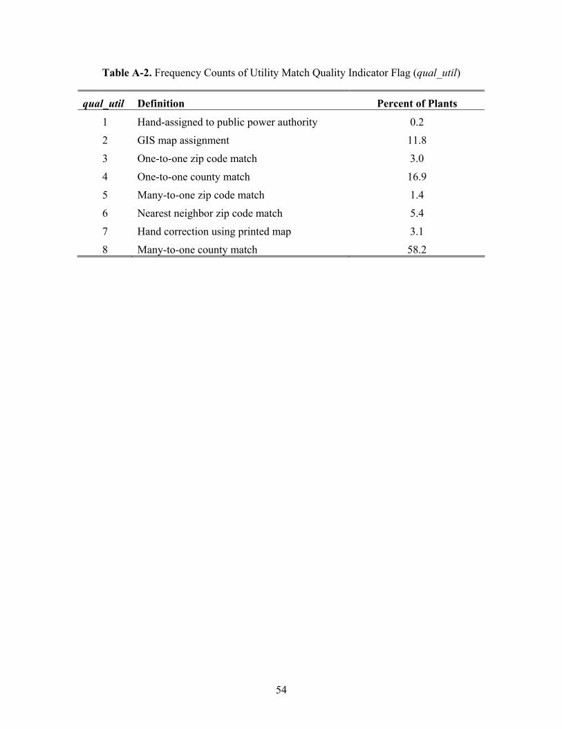
A.5 Final Matches

We construct a utility match quality indicator flag, qual_util, for each PQEM

plant-year observation. Table A-2 shows frequency counts for this flag. In total, 31.8% of

PQEM observations have a one-to-one utility match.

30 Some utilities changed ownership and/or name between 2000 (date of EIA file with utilities and utility codes) and the date the map was created. These require research using outside sources to determine the appropriate utility code. 31 State and county FIPS codes can be found on the Internet. For example, see http://www.rma.usda.gov/data/m13/fips.pdf.

53

Table A-1. List of States with Detailed Electric Utility Service Area Information

GIS Maps of Electric Utility Service Areas Kansas Kentucky Maine Minnesota Ohio Wisconsin Zip Code to Electric Utility Service Area Concordance California New York Rhode Island Printed Maps of Electric Utility Service Areas Florida Illinois Louisiana Maryland Michigan Missouri Pennsylvania South Dakota Wyoming

54

Table A-2. Frequency Counts of Utility Match Quality Indicator Flag (qual_util)

qual_util Definition Percent of Plants

1 Hand-assigned to public power authority 0.2

2 GIS map assignment 11.8

3 One-to-one zip code match 3.0

4 One-to-one county match 16.9

5 Many-to-one zip code match 1.4

6 Nearest neighbor zip code match 5.4

7 Hand correction using printed map 3.1

8 Many-to-one county match 58.2

55

Technical Appendix B: Industry Codes

B.1 1963 and 1967

The variable newind for 1963 and 1967 is initially created as: newind = OIND

(original industry code). However, the OIND codes appear to contain a combination of

1963/67 SIC codes and 1972 SIC codes. For this reason, we apply codes based on PPN

matches to 1972-1975 for as many observations as possible. We can match in industry

codes for close to 47% of the observations in the 1963 CM and just over 62% of the

observations in the 1967 CM.

Codes that cannot be matched in using 1972-1975 are assigned as newind = OIND

with corrections. Two sets of corrections are made to the OIND codes. First, corrections

are made to OIND according to information from Davis, Haltiwanger, and Schuh, 1996

(DHS). Table A-1 shows the DHS industry corrections. Note that we do not use two of

the DHS corrections: 3391 into 3399 and 3392 into 3399. Additional corrections were

added to account for changes from the 1963/67 SIC classification system to the 1972 SIC

classification system that were not included in the DHS table (designed for use from

1972-1986). Table A-2 shows these corrections for industries that could be assigned in a

simple way.32 Only about 270 (0.2%) plant-year observations required corrections from

these tables in 1963 and 1967. For splitter industries, we randomly assign plants from the

1963/67 industry that splits to the 1972 industry based on the fraction of plants in the

industry in 1972. A simple example is shown below.

• 1963/67 industry A splits into 1972 industries B and C.

• Let NX = the number of plants in industry X in 1972.

32 The corrections in Table B-1 are based on the industry concordance table for 1967 to 1972 SIC codes found in Appendix B of the 1972 Census of Manufactures publication.

56

• Let ( )CB

B

NNNZ+

= .33

• Let Q = random number between in the range [0,1] assigned to a plant in industry A in 1963/67.

• If ZQ ≤ , then assign the plant to industry B. Otherwise, assign the plant to industry C.

Approximately 3.6% (roughly 4,100) of total plant-year observations in 1963 and 1967

had industry codes assigned with the methodology described above.

B.2 1972-1986

For 1972-1986, the variable newind is also initially created as: newind = OIND.

As in 1963 and 1967, additional corrections are made to OIND according to the DHS

corrections shown in Table A-1. 1972 also contains a significant number of industry

codes in OIND that are 1987 SIC codes. Corrections shown in Table A-3 are applied to

these codes.34 We made industry corrections from these tables to approximately 1,400

(0.2%) plant-year observations from 1972 to 1986.

B.3 1987-2000

For 1987-1997, the variable newind is initially created as: newind = IND

(tabulated industry code). However, North American Industrial Classification System

(NAICS) codes are introduced to the ASM in 1998. The IND variable contains NAICS

codes in 1998-2000. Therefore, the 1998-2000 values of newind are created using

different methods. The method for 1998 and 1999 is simple; the variable OIND contains

the 1987 SIC code so newind = OIND. The method we use to create newind in 2000 is a

bit more complicated. The 2000 values of newind are based on PIND (processing

33 Note that simple (shown in Tables B-1 and B-3) corrections are made to 1972 SIC codes and only good codes are kept when creating the Z variable. 34 The 1987 SIC manual is the source of the corrections in Table B-3. It is not clear how 1987 SIC codes ended up in the OIND variable in 1972.

57

industry code) instead of IND or OIND. The variable newind is equal to PIND if PIND is

less than 10,000. If PIND is greater than or equal to 10,000, then newind is equal to the

substring containing the first four digits of PIND. Further, if this method yields an invalid

industry code, newind is taken from the most recent year containing a valid 1987 SIC

code for that plant. We only do this for roughly 400 (0.2%) of plant-year observations in

1998 to 2000.

The Asbestos industry (3292) completely disappears from the ASM in 1994-1996

and then reappears. We correct for this in the PQEM by assigning all plants that are in

industry 3292 in any of 1990-2000 to be in 3292 in all of 1990-2000. This is not a perfect

solution. There are very few plants in the Asbestos industry from 1992 to 1997. For some

purposes, a researcher may want to consider combining the Asbestos industry with

another industry similar in nature for post-1986 years.

There are 458 industries in years 1987 through 1998. In 1999, 4 industries drop

out. They are 2411 (Logging), 2711 (Newspapers: Publishing, or Publishing and

Printing), 2721 (Periodicals: Publishing, or Publishing and Printing), and 2741

(Miscellaneous Publishing). In 2000, one additional industry drops out, 2731 (Books:

Publishing, or Publishing and Printing). These industries drop out of manufacturing as a

result of the switch from SIC to NAICS. Therefore, they are not included in the

population for the ASM.

58

Table B-1. DHS Industry Corrections

Source: Page 222 in Davis, Haltiwanger, and Schuh (1996) * Note there are two DHS corrections we do not use. According to the 1967 to 1972 SIC code mapping, 1967 industry 3391 compares directly to 1972 industry 3462 and 1967 industry 3392 compares directly to 1972 industry 3463.

Old Industry Corrected Industry Discontinuous Industries

2794 2793 3672 3671 3673 3671

Miscoded Industries 2015 2016 2031 2091 2042 2048 2071 2065 2072 2066 2093 2076 2094 2077 2317 3317 2433 2439 2443 2449 2689 2649 3323 3325 3391* 3399 3392* 3399 3461 3466 3472 3743 3481 3496 3578 3579 3614 3674 3642 3646 3716 3713 3722 3724 3729 3728 3741 3743 3791 2451

59

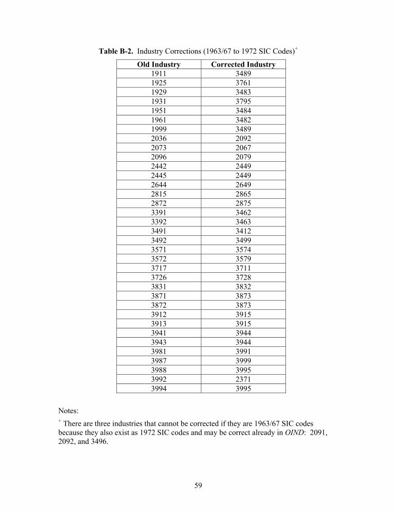
Table B-2. Industry Corrections (1963/67 to 1972 SIC Codes)+

Notes: + There are three industries that cannot be corrected if they are 1963/67 SIC codes because they also exist as 1972 SIC codes and may be correct already in OIND: 2091, 2092, and 3496.

Old Industry Corrected Industry 1911 3489 1925 3761 1929 3483 1931 3795 1951 3484 1961 3482 1999 3489 2036 2092 2073 2067 2096 2079 2442 2449 2445 2449 2644 2649 2815 2865 2872 2875 3391 3462 3392 3463 3491 3412 3492 3499 3571 3574 3572 3579 3717 3711 3726 3728 3831 3832 3871 3873 3872 3873 3912 3915 3913 3915 3941 3944 3943 3944 3981 3991 3987 3999 3988 3995 3992 2371 3994 3995

60

Table B-3. Industry Corrections (1987 SIC Codes in 1972)

Old Industry Corrected Industry 2053 2038 2064 2065 2326 2328 2656 2654 2671 2641 2672 2641 2673 2643 2674 2643 2675 2645 2676 2647 2677 2642 2678 2648 2835 2831 2836 2831 3052 3041 3053 3293 3061 3069 3081 3079 3082 3079 3084 3079 3089 3079 3363 3361 3365 3361 3366 3362 3556 3551 3596 3576 3663 3662 3669 3662 3827 3832 3845 3693

61

Technical Appendix C: Identification of ASM Plants in the 1967 CM

We examined the 1967 CM publications for information on how the ASM sample

was selected and how many plants were in the actual ASM sample. We found the

following useful information.

• The 1967 ASM reporting panel was comprised of approximately 61,000 plants.

• The ASM sample constitutes “about one-fifth of the plants but with complete

coverage of all large ones.”35 (Source: Census of Manufactures, 1967

publication)

• The certainty cases in the ASM include, in general, “all plants of companies with

at least one manufacturing plant with 100 employees or more (250 employees or

more in the apparel manufacturing and printing and publishing industries).”

(Source: Census of Manufactures, 1967 publication)

We define ASM plants in the 1967 CM in the following way. A plant is an ASM

plant if one or more of the following three conditions are met:

1. The plant is a certainty case.

2. The plant has unique values within a four-digit SIC industry for the following

ratios of CM variables: CP/TVS, WW/SW, EE/CP, PH/PW and PW/WW.

3. If, after applying criteria 1 and 2, the plant’s four-digit SIC industry - total

employment class category still contains too few plants and the plant has unique

35 There are 305,643 manufacturing plants in the 1967 CM, one-fifth of this is 61,128, which matches the estimate given above.

62

values within a four-digit SIC industry for any four of the following six ratios of

ASM variables: CP/TVS, WW/SW, EE/CP, PE/SW, PH/PW and PW/WW. 36

C.1 Certainty Cases

We use the criteria listed above with the 1967 CM value of TE to determine if a

plant is a certainty case. Clearly, the creators of the 1967 ASM sample did not have this

value of TE when they chose the ASM cases. However, the 1967 CM value of TE is

probably a fairly good proxy for the total employment variable used to choose the ASM

certainty cases. There are 45,741 certainty cases. This is a good core of plants that are

likely ASM plants. However, this number is roughly 15,000 plants short of the true

number of ASM plants.

C.2 Dunne Ratio Method

Dunne (1998), an internal CES memo on 1987 and 1992 imputes, offers a

possible suggestion of how to identify imputed (non-ASM) cases in the CM. He discusses

“typical” imputation patterns in the data. Further, he says that in 1987 and 1992, Census

imputed a “common ratio to non-respondent non-ASM cases for each four-digit

industry.” Dunne examines several ratios in 1987 and 1992, focusing on the ratio

CM/TVS (cost of materials / total value of shipments). He looks for repeated occurrences

of the same value of the ratios within four-digit industries. He states that plants with these

repeated ratios are likely imputed cases. While we make use of the Dunne ratio method,

we recognize that imputation procedures at the U.S. Census Bureau may have been very

36 Total employment classes are defined from 1 to 5 as follows: 1-19 employees, 20-49 employees, 50-99 employees, 100-249 employees and 250 or more employees. The number of plants in a four-digit SIC industry-total employment class category must be high enough that the created ASM sample weight is less than or equal to 200. See Section 5 for information on the creation of ASM sample weights in 1967.

63

different in 1967 than in 1987 and 1992. Also note, the variable CM is not available in

the 1967 CM so we use CP (cost of materials and parts) instead.

We examined six ratios in an attempt to identify 1967 ASM plants.

1. CP/TVS – cost of materials and parts / total value of shipments

2. WW/SW – production workers wages / total salaries and wages

3. PH/PW – total plant hours / average number of production workers

4. PE/SW – quantity of purchased electricity / total salaries and wages

5. EE/CP – expenditures on electricity / cost of materials and parts

6. PW/WW – average number of production workers / production workers wages

We chose ratios 1-3 based on the results in Tim Dunne’s 1998 memo. We chose ratio 4

because PE was imputed for non-ASM cases. We chose ratios 5 and 6 because they do

not include any potential administrative record variables.37 Further, we think that CP, EE,

PW, and WW are likely to have low item impute rates because they should be fairly easy

for the manager of a plant to learn and report.

C.3 Coverage Considerations

ASM sample weights have a maximum value of 200 in each of the several years

following 1967 (1972-1993). Therefore, we force our sample to be such that there are no

sample weights over 200. We also developed a method of creating ASM sample weights

for 1967.38

37 TVS and SW could potentially be in the administrative record. If administrative record information for “whole” impute cases was added to the 1967 CM data, it is possible that unique ratios will occur even for “whole” impute cases if the ratios involve administrative record data such as TVS or SW. [Recall that the standard imputation method is Xet = PAYROLLet (Xit/PAYROLLit).] Thus, ratios 1, 2, and 4 may not yield clear results for identifying ASM plants. 38 See Section 5 for a full description of this method.

64

C.4 Choosing the Final Set of 1967 ASM Plants

First, we create several variables to examine repeats of our six chosen ratios

within four-digit SIC industries. Then, we create an ASM sample based on the method

described in criteria 1 and 2 in Part B of this section. However, this sample contains

several plants with sample weights of over 200. These high weights are the results of

selecting too few plants in the smallest total employment class in some four-digit SIC

industries. To solve this problem, we add plants from the smallest total employment class

in problematic four-digit SIC industries. Plants are added to the ASM sample if they have

unique ratios for any four of the following six ratios of ASM variables: CP/TVS,

WW/SW, EE/CP, PE/SW, PH/PW and PW/WW. This method yields 62,900 ASM plants.

65

Technical Appendix D: Creation of ASM Sample Weight for 1963 and 1967

ASM sample weights are not available on the 1963 and 1967 CM plant-level data

files. This section describes the method we use to estimate ASM sample weights for the

1963 and 1967 CM surveys. Plant-level data files for all other years already contain ASM

sample weights (WT).

D.1 1963 Sample Weights

We use a simple algorithm to estimate ASM sample weights in 1963. The steps of

the algorithm are listed below.

1. Identify ASM cases: ASM cases in the 1963 CM are identified by the plant type

(ET) flag equal to zero.

2. Assign weights to ASM certainty cases: All ASM certainty cases are given a

weight equal to one. The 1963 CM publication states that all plants of companies

with 100 or more employees were ASM certainty cases. (Source: Census of

Manufactures, 1963 publication)

3. Assign weights to ASM non-certainty cases: Non-certainty cases are assigned a

weight of one over the probability of selection. We define the probability of

selection based on the following three total employment (TE) classes, by 4-digit

industry: 1-19, 20-49, and 50-99 employees. For example, if there are 20 ASM

plants and 100 CM plants with TE of 1-19 in industry 2011, the probability of

selection of each of the 20 ASM plants is 1/5.

D.2 1967 Sample Weights

The algorithm we use to estimate ASM sample weights in1967 is very similar to

the algorithm used for 1963. The steps of the 1967 algorithm are as follows:

66

1. Identify ASM cases: Unlike the 1963 ASM cases, ASM cases in the 1967 CM are

not immediately identifiable; all plants have ET equal to one. Our criteria for

choosing ASM cases in the 1967 CM are described in the previous section.

2. Assign weights to ASM certainty cases: All ASM certainty cases are given a

weight equal to one. The 1967 CM publication states that the certainty cases in

the ASM include, in general, “all plants of companies with at least one

manufacturing plant with 100 employees or more (250 employees or more in the

apparel manufacturing and printing and publishing industries).” (Source: Census

of Manufactures, 1967 publication)

3. Assign weights to ASM non-certainty cases: Non-certainty cases are assigned a

weight of one over the probability of selection. We define the probability of

selection based on the following four total employment (TE) classes, by 4-digit

industry: 1-19, 20-49, 50-99, and 100-249 employees.

67

Technical Appendix E: Geography Codes

This section describes changes we made to the state and county FIPS codes to

make them correct and consistent for in the PQEM.

E.1 Creation of a Unique County Identifier

The PQEM contains FIPS county and state codes for each plant-year observation.

The FIPS county code is repeated across states. Therefore, we combine the FIPS state and

county codes to get a single county identifier. We create a variable called cyfstn that is

unique to each county-state combination by concatenating the 2-digit FIPS state code to

the end of the 3-digit FIPS county code. The cyfstn variable is a character variable of

length five.39

E.2 Hawaii FIPS State Code Correction: 1963-1988

There are several state identifiers on the ASM and CM plant-level data files: FIPS

state code (FIPSST), Census state code (CENST), state name (STATE), and state postal

abbreviation (POSTALST). For the years 1963-1988, the FIPS state code for Hawaii

(FIPSST = 15) never appears on the ASM or CM files.40 While Hawaii is not a big

manufacturing state, it does have some manufacturing plants, such as food canning

plants. This problem was identified on previous versions of the ASM and CM plant-level

data files by Randy Becker. Becker (1999) describes the Hawaii problem and a method

for correcting it on the 1963-1987 CM files.

Following Becker (1999), we use the algorithm below to correct state codes from

1963-1988.

39 The cyfstn variable is re-created after the corrections described below to the FIPS county and state code variables. 40 The STATE for Hawaii (“Hawaii”), the POSTALST for Hawaii (“HI”), and the CENST for Hawaii (“15”) also do not appear in 1963-1988.

68

• For 1963-1981 and 1983-1985, CENST is correct on previous versions of the ASM

and CM files. For Hawaii, CENST = 95. The fix is straightforward: drop CENST

from the PQEM (for the problem years), merge on CENST from the previous versions

of the files by year and PPN, and then if CENST = 95 set FIPSST = 15.

• For 1982 and 1986-1988, the fix is more complicated. In these years, FIPSST,

CENST, and REG (census region) all have problems. There is a fix file,

STATEFIX.sas7bdat, available for the CM years. This file contains the variables

shown in Table D-1 for the years 1972, 1977, 1982, and 1987.

• In 1982 and 1987, the values of FIPSST are corrected directly by merging the

STATEFIX file to the PQEM by year and PPN. This match is checked by comparing

the TVS, TE, and IND variables. 41

• We use matches from surrounding years to correct the bad FIPSST variable in 1986

and 1988.

E.3 FIPS County Code Problem: 1986

The FIPS county code (COU) variable in the 1986 ASM plant-level data file does

not contain the FIPS county code (as of March 2005). It actually contains the last 3 digits

of the place code variable (PLAC). The correct county code is contained in the first 3

digits of the SMSA field.

E.4 County Concordance Over Time

According to Becker (1999), there are two main areas of concern related to

concordance over time for FIPS county codes. First, FIPS county codes have changed

over time. For instance, between 1967 and 1972, there was a major change in the codes.

41 The real SMSA code is “lost” in 1986 (missing in the PQEM). However, it could be mapped in using the correct state and county codes.

69

To make room for future additions, “space” was added between FIPS county codes. The

new codes were usually, though not always, defined according to (1).

New FIPS County Code = (Original FIPS County Code)*2 – 1 (1)

There are also cases of counties being combined or split up. The second major concern

with county data is the changing of boundaries over time. Unfortunately, if this boundary

change is not reflected in a simple FIPS county code change, we will not correct for it.

Randy Becker provided us with a county concordance program for the CM years.

We modified this program in two ways. First, we modified the program to include ASM

years. Second, we added corrections for Alaska to the program.42 We then applied the

program to our database to achieve the best possible county concordance over time.

E.5 Concordance with EIA Utility Data Counties

EIA utility data, described in Section 2.2, is merged to the PQEM by county. We

want utility data for every plant-year observation. Therefore, we need concordance

between the counties in our database and the counties in the EIA data file. There are 13

counties in the PQEM that do not have matches to the EIA data file. These counties are

actually independent cities with their own FIPS county codes. We examined each of these

individually to determine the utility that most likely provides their electricity.43 We then

42 The original program did not include corrections for Alaska beyond the general correction for the 1967 to 1972 FIPS county code change. As of 2000, there were 27 FIPS county-equivalents in Alaska. Table E-2 shows a list of the Alaska county-equivalents. Some of these county-equivalents were split out from other county-equivalents. Therefore corrections need to be made for concordance over time. Following the method in Randy Becker’s program, the counties are put back together into their former county. Additionally, there were several county-equivalents in the early years (1963, 1967) of the CM that were later added to other county-equivalents. Table E-3 shows the corrections we include in our database. Finally, we should note in the 1960s there are plants listed in county 001 for Alaska. Most of the occurrences are in 1963, though there are a few in 1967. This was a large division that was later separated into several county-equivalents. We feel it is too large to put all of the county-equivalents back together. Therefore, we use later years to determine the location of the plant. If the plant did not appear in later years (there are only around 30 such plants), we drop those plant-year observations. 43 We looked the cities up on the Internet to determine the utility currently serving them. As a check, we looked at the utilities serving the surrounding counties as well. In a couple of cases, there was more than

70

added them to the EIA data file. Table D-4 shows a list of these counties and the utilities

they were assigned. There are roughly 11,500 (0.63%) plant-year observations located in

these counties over all years of the PQEM.

E.6 Consistent State Code Requirement for Plants

Finally, we require that a plant does not change states over the period of the

PQEM. We use PPN (permanent plant number) as the plant identifier. A PPN should be

assigned to a single plant location regardless of ownership or industry. If a manufacturing

plant relocates, it should be assigned a new PPN. Therefore, if county and state

boundaries are stable over time, a given PPN should have the same FIPS county and state

codes throughout our sample period. However, we know that county boundaries do

change over time. As noted previously, we cannot capture these boundary changes if they

are not reflected in a simple FIPS county code change. Therefore, we allow the county of

a given PPN to vary over our sample period. However, since state boundary changes are

very rare, we do not allow the state of a given PPN to change over our sample period.

There were a small number of occurrences of state changes over time for a given PPN in

our database. We used the following algorithm to create consistent FIPS state codes over

time in our database.

1. Flag all plants for which the FIPS state code changes during our sample period.

2. For the flagged plants, assign the cyfstn that appears in the most years to that plant

in all years.44 If there is a tie, assign the cyfstn that appeared most recently to the

plant in all years.

one possible utility. For these cases, we picked the utility that served the largest number of surrounding counties. 44 We change the cyfstn variable rather than the FIPS state code alone because changing the FIPS state code alone would lead to non-existent county-state combinations in cyfstn.

71

3. For flagged plants, correct the FIPS state code to match the corrected cyfstn.

This correction changes the cyfstn and FIPS state code variable for 0.57% (roughly

10,000) of our plant-year observations. The number of corrected observations is spread

fairly evenly across years, ranging from around 200 to 500 corrected observations per

year.

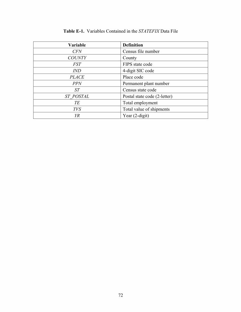
72

Table E-1. Variables Contained in the STATEFIX Data File

Variable Definition CFN Census file number

COUNTY County FST FIPS state code IND 4-digit SIC code

PLACE Place code PPN Permanent plant number ST Census state code

ST_POSTAL Postal state code (2-letter) TE Total employment TVS Total value of shipments YR Year (2-digit)

73

Table E-2. Alaska FIPS County-Equivalents

FIPS County Code County 013 Aleutians East 016 Aleutians West 020 Anchorage 050 Bethel 060 Bristol Bay 068 Denali 070 Dillingham 090 Fairbanks North Star 100 Haines 110 Juneau 122 Kenai Peninsula 130 Ketchikan Gateway 150 Kodiak Island 164 Lake and Peninsula 170 Matanuska-Sustina 180 Nome 185 North Slope 188 Northwest Arctic 201 Prince of Wales-Outer Ketchikan 220 Sitka 232 Skagway-Hoonah-Angoon 240 Southeast Fairbanks 261 Valdez-Cordova 270 Wade-Hampton 280 Wrangell-Petersburg 282 Yakutat 290 Yukon-Koyukuk

74

Table E-3. Corrections to FIPS County-Equivalents

Original FIPS

County Code

Original County

Corrected FIPS County

Code

Corrected County

013 Aleutians East 010 Aleutians 016 Aleutians West 010 Aleutians 030 Angoon 231 Skagway-Yakutat-Angoon 040 Barrow-North Slope 185 North Slope 080 Cordova-McCarthy 261 Valdez-Cordova 164 Lake and Peninsula 070 Dillingham 230 Skagway-Yakutat 231 Skagway-Yakutat-Angoon 232 Skagway-Hoonah-Angoon 231 Skagway-Yakutat-Angoon 282 Yakutat 231 Skagway-Yakutat-Angoon

75

Table E-4. Utilities Individually Assigned to Counties

State FIPSST County COU Assigned Utility (Utility Code) MO 29 St. Louis city 510 Union Electric Company (19436) VA 51 Bristol city 520 Bristol Utilities Board (2248) VA 51 Danville city 590 Danville City (4794) VA 51 Franklin city 620 Franklin City (6715) VA 51 Galax city 640 Appalachian Power Company (733) VA 51 Harrisonburg city 660 Harrisonburg City (8198) VA 51 Lynchburg city 680 Appalachian Power Company (733) VA 51 Martinsville city 690 Martinsville City (11770) VA 51 Norton city 720 Old Dominion Electric Power

(10171) VA 51 Radford city 750 Radford City (15619) VA 51 Roanoke city 770 Appalachian Power Company (733) VA 51 South Boston city 780 Virginia Electric & Power (19876) VA 51 Williamsburg city 830 Virginia Electric & Power (19876)

76

Technical Appendix F: TVS Outliers

F.1 Data Filter

A plant-year observation is flagged for TVS imputation if the following criteria are met:

(1) Payroll (SWt) < 2% of TVSt and

(2) TVSt > median of 4-digit SIC industry TVS for year t and

(3) • If t = 1963:

Absolute value of (log(TVSt+5) – log(TVSt)) > 5 • If t =1967:

Absolute value of (log(TVSt+5) – log(TVSt)) > 5 and45 Absolute value of (log(TVSt-5) – log(TVSt)) > 5

• If t =1972: Absolute value of (log(TVSt+1) – log(TVSt)) > 1 and45 Absolute value of (log(TVSt-5) – log(TVSt)) > 5

• If 1973 ≤ t ≤ 1999: Absolute value of (log(TVSt+1) – log(TVSt)) > 1 and45 Absolute value of (log(TVSt-1) – log(TVSt)) > 1

• If t =2000: Absolute value of (log(TVSt-1) – log(TVSt)) > 1

We flag a total of 105 plant-year observations for TVS imputation, including the 1963 case described above. Not surprisingly, we flag more observations for TVS imputation in the two end years, 1963 and 2000.

F.2 Imputation Method

For observations we flag for TVS imputation, we perform a simple imputation based on the plant’s TVS to SW ratio in the two (if available) surrounding years. We use the following procedure to impute TVS.

(1) Calculate the ratio of TVS to SW in each year

t

tt SW

TVSSWTVSrat =__

(2) Calculate TVS_SW_avg

• If t = 1963: 5____ += tt avgSWTVSavgSWTVS

45 We also tried using an “or” condition here. However, we flag some cases we should not flag when we do this. For example, we flag a lot of cases for imputation where there is a big jump in TVS from the previous year where TVS is at approximately the same level in later years (e.g., the year after entry).

77

• If t = 1967:

( )55 ____21__ +− += ttt avgSWTVSavgSWTVSavgSWTVS

• If t = 1972:

( ) ( )15 __54__

51__ +− += ttt avgSWTVSavgSWTVSavgSWTVS

• If 1973 ≤ t ≤ 1999:

( )11 ____21__ +− += ttt avgSWTVSavgSWTVSavgSWTVS

• If t = 2000: 1____ −= tt avgSWTVSavgSWTVS

(3) Calculate corrected TVS, TVS_CORR

ttt avgSWTVSSWCORRTVS __*_ =

prices and quantities of electricity in the u.s ...econ-server.umd.edu/~haltiwan/pqem.pdfpreliminary...

Documents