price competition with repeat, loyal buyers · price competition with repeat, loyal buyers ......

Price competition with repeat, loyal buyers

Eric T. Anderson & Nanda Kumar

Received: 10 February 2006 /Accepted: 5 March 2007 /Published online: 13 September 2007# Springer Science + Business Media, LLC 2007

Abstract Extant theoretical models suggest that greater consumer loyalty increasesa firm’s market power and leads to higher prices and fewer price promotions(Klemperer, Quarterly Journal of Economics 102(2):375–394, 1987a, EconomicJournal 97(0):99–177, 1987b, Review of Economic Studies 62(4):515–539, 1995;Padilla, Journal of Economic Theory 67(2):520–530, 1995). However, in somemarkets large, national brands that are able to generate more consumer loyalty thantheir rivals offer lower prices and promote more frequently. In this paper, we developa two-period game-theoretic, asymmetric duopoly model in which firms differ intheir ability to retain repeat, loyal buyers. In this market, we demonstrate that it isoptimal for a firm that generates more loyalty to offer a lower average price andpromote more frequently than a weaker competitor. Numerical analysis of a moregeneral infinite period version of this asymmetric model leads to three additionalresults. First, we show that there is an inverted-U relationship between a weak firm’sability to attract repeat, loyal consumers and strong firm profits. Second, we show thatthe relative ability of firms to attract repeat buyers affects whether serial andcontemporaneous price correlations are positive or negative. Finally, we highlight theeffect of dynamics on firms’ expected prices and profits.

Keywords Price promotions . Promotion depth and frequency . Loyalty

JEL Classifications C70 . C72 . D40 . D43 . L00 . L11 .M21 .M31

Quant Market Econ (2007) 5:333–359DOI 10.1007/s11129-007-9023-7

The paper has benefited from discussions with Birger Wernerfelt, Ram Rao and Sridhar Moorthy. Theusual disclaimer applies.

E. T. Anderson (*)Kellogg School of Management, Northwestern University, 2001 Sheridan Road,Marketing Department, 4th Floor, Evanston, IL 60208, USAe-mail: [email protected]

N. KumarSchool of Management, UT Dallas, SM 32, P.O. Box 830688, Richardson, TX 75083-0688, USAe-mail: [email protected]

1 Introduction

Numerous marketing studies document that consumer loyalty or state dependencevaries across consumers, brands, and categories (Guadagni and Little 1983;Seetharaman et al. 1999). Extant theoretical models suggest that greater consumerloyalty increases a firm’s market power and leads to higher prices and fewer pricepromotions (Klemperer 1987a, b, 1995; Padilla 1995). However, in some marketslarge, national brands that are able to generate more consumer loyalty than theirrivals offer lower prices and promote more frequently. For example, using the ERIMdata researchers find that peanut butter and stick margarine are two categories inwhich many consumers exhibit state dependence (Seetharaman et al. 1999) and largeshare brands have more state dependence or loyalty (Van Oest and Frances 2003).Surprisingly, the largest national brands in these categories, Peter Pan (peanut butter)and Parkay (stick margarine), offer a lower average price and more frequentpromotions than rival national brands.

Such pricing strategies are inconsistent with predictions from the extant literaturein economics and marketing. The economics literature has emphasized thatswitching costs or state dependence should lead to higher prices (Klemperer1987a, b, 1995; Padilla 1995), but in the previous examples we observe the opposite.In marketing, the theoretical literature on price promotions has examinedcompetition between weak brands and strong brands, which are assumed to havemore loyal consumers (Narasimhan 1988; Raju et al. 1990; Lal 1990; Rao 1991).However, these models predict that the optimal strategy for a strong brand is to offerinfrequent, deep discounts or frequent, shallow discounts. In sum, the existingliterature cannot explain why a brand that creates more consumer loyalty than its rivalswould compete by offering a lower average price and more frequent promotions.

In this paper, we develop a dynamic, game theoretic model that offers anexplanation for this pricing behavior. Similar to past research on state dependence orswitching costs, we allow consumers who are initially indifferent to become loyal toa brand. However, the key difference in our model is that we assume firms areasymmetric in their ability to create consumer loyalty or state dependence. In ourduopoly model we refer to a firm as strong if it converts a greater fraction of trialpurchasers into repeat, loyal consumers; analogously, we refer to the competing firmas weak. In packaged goods, an asymmetry in each firm’s ability to create statedependence is consistent with the notion that some brands are able to create morefavorable purchase experiences that lead to consumer loyalty. Asymmetries in statedependence may also be present in business markets. For example, a firm that offersa proprietary, closed software system may be able to create lock-in or statedependence while rivals who sell open software systems may not have the samedegree of loyalty.

Our assumption that loyalty is in-part created by a firm’s pricing strategyendogenizes the size of a firm’s loyal base of consumers. This creates a trade-offbetween investing and harvesting as a firm optimizes its pricing strategy. To invest increating a loyal base of consumers, a firm may offer a low price that attracts newconsumers and some of these buyers may become loyal. In contrast, once a firmestablishes a large base of loyal consumers they can harvest the value created by

334 E.T. Anderson, N. Kumar

charging a high price.1 In every period, a firm must assess the market to determinewhether it is optimal to invest or harvest.

A key insight from the model is that the incentive to invest and harvest differs forstrong and weak firms. If a weak firm attracts few repeat, loyal buyers then the onlybenefit of a low price is the current increase in market share. A strong firm thatattracts more loyal consumers benefits from a low price in both the current periodand future periods. In a two period model, we show analytically that the incentive tocreate future loyalty may lead a strong firm to offer a lower average price andpromote more frequently than a weak firm. As shown in Table 1, this prediction isconsistent with the pricing strategies used by Peter Pan peanut butter and Parkaymargarine in Springfield, MO. Both leading brands offer a lower average price,promote more frequently, and offer a higher percentage discount compared to thesecond largest brand in the category.

Our analysis of a more general infinite period version of this asymmetric modelallows us to obtain three additional results numerically. First, we show that there isan inverted-U relationship between the weak firm’s ability to attract repeat, loyalconsumers and the strong firm’s profits. Second, we show that the relative ability offirms to attract repeat buyers affects whether serial and contemporaneous pricecorrelations are positive or negative. Finally, we highlight the effect of dynamics onfirms’ expected prices and profits. Next, we briefly discuss each result.

The inverted-U relationship in profits can be explained by two competing effects.When a competitor is able to capture more repeat, loyal consumers there is a directloss of market share for the rival. But, an increase in the number of loyal customersraises all firms’ prices. When a competitor is very weak, the loss in market share issmall compared to the benefit of increased prices and both firms’ profits increase.However, as the rival firm attracts more loyal buyers, the loss in market share is thedominant effect and own firm profits decrease. This result suggests that when firmsare very asymmetric in their ability to attract repeat, loyal buyers, a strong firm maywant to accommodate a weaker rival’s attempts to increase repeat purchases. As thefirms become symmetric, each firm should react aggressively to either firm’s attemptto attract repeat, loyal buyers.

Our model also shows that firms’ relative ability to attract repeat, loyal consumersdetermines whether serial and contemporaneous price correlations are positive ornegative. When firms are symmetric and attract a similar number of repeat buyers,then both contemporaneous and serial price correlations are negative. In practice,this is analogous to firms engaging in asynchronous, high-low pricing strategies (Lal1990). When the weak firm attracts few repeat, loyal consumers the weak firm’sserial and contemporaneous price correlations are positive. The positive correlationoccurs because of the weak firm’s incentive to mimic the behavior of the strong firm(i.e., strategic price effect).

Our results on price correlations complement findings from extant promotionmodels. In static models, price correlations are zero (Shilony 1977; Varian 1980;

1 We consider myopic consumers who do not anticipate that prices may increase in future periods. Thisassumption simplifies the analysis but we expect the intuition from our model to extend to a setting withforward-looking consumer behavior. This may require a different model formulation.

Price competition with repeat, loyal buyers 335

Narasimhan 1988; Raju et al. 1990; Lal 1990; Rao 1991) and hence cannot speak tothese issues. The price cycles literature (Conlisk et al. 1984; Sobel 1984; Villas-Boas2004a, 2006) predicts that a monopolist will offer periodic promotions, whichimplies negative serial correlation. In our model, serial correlation of the strong firmis negative, which is consistent with this literature. However, our model shows thatstrategic price effects can be significant enough for the serial price correlation of aweak firm to be positive. Finally, other competitive promotion models have shownthat the contemporaneous price correlation can be either negative (Lal 1990) orpositive (Sobel 1984). In a single model, we show how one factor (i.e., the numberof repeat, loyal consumers) can determine whether price correlations are positive ornegative.

We assume that both firms in our model optimize discounted, long-run profits. Animportant question is whether firms’ concerns for future profits softens or sharpenscompetition. We find that if the firms were to set prices myopically, the expectedprofits of the weak firm would increase. In contrast, myopic pricing does notnecessarily benefit the strong firm. If the weak firm attracts few repeat, loyal buyersthen myopic pricing may decrease profits of the strong firm. We conclude that theeffect of myopic pricing depends on a firm’s relative market position (i.e., strong orweak) and on the degree of asymmetry in each firm’s ability to attract repeat, loyalbuyers.

Our model contributes to the marketing and economics literatures on switchingcosts, which have been shown to affect price levels, market attractiveness to a newentrant, and tacit collusion (Klemperer 1987a, b, 1989; Beggs and Klemperer 1992;Padilla 1995, Anderson et al. 2004). A summary of the switching cost literature isprovided in Klemperer (1995). A common force in these models is that firms mayhave an incentive to offer low prices to attract consumers and then offer higherprices in later periods when consumers face switching costs. Indeed, the strong firmin our model engages in this strategy. Two key features distinguish our model fromthe switching cost literature. First, we focus on the number of customers whobecome loyal (i.e., develop switching costs) and second, we analyze firms that differin their ability to attract repeat, loyal buyers (i.e., asymmetric firms). In contrast, atypical switching cost model analyzes the magnitude of a consumer’s switching costand considers competition between symmetric firms.

Table 1 Average price and promotion frequency

Category Brand Marketshare (%)

Averageprice

Promotionfrequency* (%)

Percentagediscount** (%)

Peanut butter Peter Pan 25 $1.80 10 10Peanut butter Jif 9 $1.85 6 6Margarine Parkay 32 $0.57 15 17Margarine Blue Bonnet 11 $0.61 13 11

*A promotion is defined as a price change of more than 5%.** Percentage discount is defined as the average percentage discount when there is a promotion.


In related papers, Villas-Boas develops two period (2004a) and infinite period(2006) dynamic models in which forward-looking consumers are initially uncertainabout how well a product fits their preferences. After a purchase experience consumerslearn about the true fit of the product. Our model assumes consumers are myopic but hasa similar feature in that some consumers are initially indifferent and a fraction of theseconsumers become loyal. While we focus on the effect of such behavior on firms’ pricingstrategies Villas-Boas focuses on “the competitive effects of the potential informationaladvantages of a product that has been tried by the consumer” (Villas-Boas 2004a, p. 142).

Our work also adds to the empirical consumer choice literature that documentsboth dynamics and state dependence in consumer preferences (Guadagni and Little1983; Erdem and Keane 1996; Mela et al. 1997; Foekens et al. 1999; Anderson andSimester 2004). Our model complements these empirical studies as we provide atheory that relates consumer dynamics to competitive behavior. In addition, ourresults provide a framework to explain empirically observed patterns of competitiveprice response (Leeflang and Wittink 1992, 1996; Kopalle et al. 1999).

The remainder of this paper is organized as follows. In Section 2 we consider atwo period model that allows us to derive our two main results analytically. InSection 3, we extend this model to an infinite horizon, overlapping generationsmodel and derive analytic expressions that fully characterize equilibrium pricingstrategies and payoffs. Because the pricing strategies involve complex analyticexpressions, many important results can only be shown through numericalsimulation. In Section 4, we present results of our numerical analysis of the infinitehorizon model. Two of these results replicate findings from the two period modeland we also present additional results on price correlations and the effect of forward-looking firm behavior. We conclude with a brief discussion in Section 5.

2 Two-period model

We consider a market with two competing firms that we label s for strong and w forweak. Each firm has zero marginal cost and sells one product over two periods tothree types of consumers: static loyal consumers, dynamic loyal consumers andswitchers. Both firms have a mass of l static loyal consumers who purchase fromtheir preferred firm as long as price is less than the reservation price (i.e., pj ≤ r.where j ∈ {s,w}). In period 1, we assume there is a unit mass of switchers whobehave myopically and purchase from the firm that offers the lowest price as long asp ≤ r. We assume that a customer who is initially a switcher may become a loyalconsumer in the subsequent period. We refer to consumers who are initiallyswitchers but become loyal as dynamic loyal consumers.

Unlike previous models of state dependence, a key assumption in our model is thateach firm differs in their ability to convert switchers into loyal consumers. We assumethat the strong brand is able to convert θs switchers into dynamic loyal consumers whilethe weak brand converts θw consumers, where θs > θw. This assumption is supported byempirical studies that show that large share brands tend to generate more statedependence (Van Oest and Frances 2003). Intuitively, one might expect a leading brandin a category, such as Tide detergent, to generate more state dependence than its rivals.


To simplify our analysis we assume that θs=1 and allow θw to vary between 0 and1. This implies that if the weak brand offers the lowest price in period 1 then θw ofthe switchers become loyal to the weak brand in period 2. In this case, the market inperiod 2 consists of l consumers who are loyal to the strong firm, l+θw consumerswho are loyal to the weak firm and (1−θw) switchers. In contrast, if the strong firmoffers the lowest price in period 1 then all switching consumers become loyal to thatfirm. The market in period 2 consists of l+1 consumers who are loyal to the strongfirm, l consumers who are loyal to the weak firm and zero switchers. Relaxing ourassumptions to allow θs<1 does not substantively change any of our main results butadds complexity to the analysis.

We solve the game by backward induction from period 2. Given our assumptions,there are two possible states in period 2 that we label state 0 and state 1. In state 0,the strong firm has θs dynamic loyal consumers while in state 1 the weak firm has θwdynamic loyal consumers. In state 0 there are no switchers, hence, both firms chargethe reservation price and the profit of each firm is: ps20 ¼ r l þ 1ð Þ and πw20 = rlwhere πijk represents the profit of firm i in period j in state k. In state 1, there is noequilibrium in pure strategies but there is a unique mixed strategy equilibrium. LetFj21(p) represent the CDF of firm j in period 2 in state 1 and assume each firm mixesover prices in the range ½p21; r�. Given that the weak brand has more loyal consumersit is easily shown that Fw21 has a mass point at p = r but the strong firm has no masspoint in its distribution. The lower bound of the support is p21 ¼ r l þ θwð Þ= l þ 1ð Þ,which is the lowest price the weak firm would offer. The equilibrium pricingstrategies of the firms in state 1 must satisfy the following conditions:

p l þ 1� θwð Þ 1� Fw21 pð Þð Þ½ � ¼ p21 l þ 1� θwð Þð Þ; ð1Þ

p l þ qw þ 1� qwð Þ 1� Fs21 pð Þð Þ½ � ¼ r l þ qwð Þ: ð2Þ

In Eqs. 1 and 2, the left hand side represents the expected second period payoff instate 1 given the rival’s mixing distribution and the right hand side represents thereservation profits of the strong and weak firm, respectively. Solving Eqs. 1 and 2we obtain the equilibrium mixing distributions in period 2 in state 1:

Fw21 pð Þ ¼ 1� l 1þ lð Þ r � pð Þ þ rθw 1� θwð Þp 1þ lð Þ 1� θwð Þ ; 8p 2 p21; r

h �ð3Þ

Fs21 pð Þ ¼ p 1þ lð Þ � r l þ θwð Þp 1� θwð Þ ; 8p 2 p21; r

h ið4Þ

We now turn to the first period strategies of both firms. Consistent with ourprevious analysis, there is no pure strategy equilibrium in period 1 and the uniqueequilibrium is in mixed strategies. While both firms have the same number of loyalconsumers in period 1 the strong firm is able to convert a greater fraction of


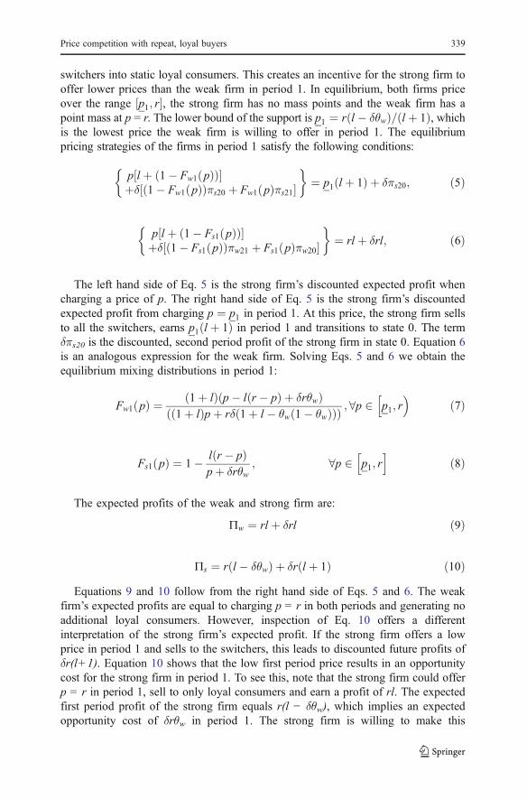
switchers into static loyal consumers. This creates an incentive for the strong firm tooffer lower prices than the weak firm in period 1. In equilibrium, both firms priceover the range ½p1; r�, the strong firm has no mass points and the weak firm has apoint mass at p = r. The lower bound of the support is p1 ¼ r l � δθwð Þ= l þ 1ð Þ, whichis the lowest price the weak firm is willing to offer in period 1. The equilibriumpricing strategies of the firms in period 1 satisfy the following conditions:

p l þ 1� Fw1 pð Þð Þ½ �þδ 1� Fw1 pð Þð Þπs20 þ Fw1 pð Þπs21½ �

� �¼ p1 l þ 1ð Þ þ δπs20; ð5Þ

p l þ 1� Fs1 pð Þð Þ½ �þδ 1� Fs1 pð Þð Þπw21 þ Fs1 pð Þπw20½ �

� �¼ rl þ δrl; ð6Þ

The left hand side of Eq. 5 is the strong firm’s discounted expected profit whencharging a price of p. The right hand side of Eq. 5 is the strong firm’s discountedexpected profit from charging p ¼ p1 in period 1. At this price, the strong firm sellsto all the switchers, earns p1 l þ 1ð Þ in period 1 and transitions to state 0. The termδπs20 is the discounted, second period profit of the strong firm in state 0. Equation 6is an analogous expression for the weak firm. Solving Eqs. 5 and 6 we obtain theequilibrium mixing distributions in period 1:

Fw1 pð Þ ¼ 1þ lð Þ p� l r � pð Þ þ δrθwð Þ1þ lð Þpþ rδ 1þ l � θw 1� θwð Þð Þð Þ ; 8p 2 p1; r

h �ð7Þ

Fs1 pð Þ ¼ 1� l r � pð Þpþ δrθw

; 8p 2 p1; rh i

ð8Þ

The expected profits of the weak and strong firm are:

9w ¼ rl þ δrl ð9Þ

9s ¼ r l � δθwð Þ þ δr l þ 1ð Þ ð10ÞEquations 9 and 10 follow from the right hand side of Eqs. 5 and 6. The weak

firm’s expected profits are equal to charging p = r in both periods and generating noadditional loyal consumers. However, inspection of Eq. 10 offers a differentinterpretation of the strong firm’s expected profit. If the strong firm offers a lowprice in period 1 and sells to the switchers, this leads to discounted future profits ofδr(l+1). Equation 10 shows that the low first period price results in an opportunitycost for the strong firm in period 1. To see this, note that the strong firm could offerp = r in period 1, sell to only loyal consumers and earn a profit of rl. The expectedfirst period profit of the strong firm equals r(l − δθw), which implies an expectedopportunity cost of δrθw in period 1. The strong firm is willing to make this


investment since the discounted period 2 payoff in state 0 exceeds the discountedexpected payoff in state 1 by δr(1 − θw(1 − θw))(1+l). We conclude that the strongfirm’s pricing strategy is analogous to loss-leader pricing. The strong firm offers lowprices in period 1 and incurs an opportunity cost but recoups this loss in period 2.

Our two period model yields two key results. First, we show that the incentive tocreate repeat, loyal buyers results in the strong firm offering lower average pricesand promoting more frequently. We state this formally as:

2.1 Result 1

(a) The expected price of the strong firm is less than the weak firm.(b) The strong firm promotes more frequently than the weak firm.

As shown in the Appendix, Result 1a follows from stochastic dominance of thefirms’ pricing strategies. In period 1, the strong firm has an incentive to offer lowerprices to attract switchers. In period 2, both firms charge the same price in state 0and the weak firm has more loyal consumers and charges a higher price in state 1.Together, this implies that the expected price of the strong firm is lower than theweak firm.

Consistent with previous theoretical price promotion models, we interpret pricesof p < r as promotions (Narasimhan 1988; Raju et al. 1990). Result 1b shows thatthe strong firm promotes more frequently than the weak firm. In period 1, the strongfirm always promotes but the weak firm may not promote. In period 2, neither firmpromotes in state 0 and the strong firm promotes more frequently in state 1. Thisimplies that the strong firm promotes more frequently than the weak firm.

A second key result from our model is how the weak firm’s ability to build a baseof loyal consumers, as measured by θw, affects the strong firm’s profits. Our modelillustrates that θw affects the strong firm’s profits in two ways and this is bestillustrated by considering payoffs in state 1.

2.2 Result 2

The expected profits in state 1 of the strong firm are increasing for low values of θwand decreasing for large values of θw .

Using the right hand side of Eq. 1, one can show that the expected profit of thestrong brand in state 1 equals p21 l þ 1� θwð Þð Þ. Substitution and simplificationyields πs20 ¼ r l2 þ l þ θw � θ2w

� ��l þ 1ð Þ. Hence, there is an inverted-U relationship

between the strong firm’s profits and the weak firm’s ability to create loyalty. For θw<0.5 the strong firm’s profits are increasing in θw and for θw>0.5 the strong firm’sprofits are decreasing in θw.

In Result 2, two forces are at work and we refer to these as the direct effect andstrategic effect. An increase in θw results in more repeat buyers for the weak firm anda direct loss in market share for the strong firm. Thus, the direct effect is alwaysnegative for the strong firm. But, an increase in the number of loyal consumers raisesthe expected price of the weak firm. Since prices are strategic complements, anincrease in the expected price of the rival allows the strong firm to raise its expected


price. The strategic effect is always positive. When θw is small, the strategic effectdominates and the strong firm’s profits are increasing in θw. However, when θw islarge, the direct effect dominates and the expected profit of the strong firm isdecreasing in θw.

The extant literature on price promotions and state dependence has focused on thenumber of static loyal consumers, l, and the degree to which a consumer is loyal to abrand. The latter is often measured as a switching cost, c, which is the price premiuma consumer is willing to pay for the preferred brand. Results 1 and 2 contribute to theextant literature by highlighting that changes in l and c have a different impact thanchanges in a firm’s ability to create dynamic loyal consumers, θj.

Static promotion models show that a firm with more loyalty offers either deep,infrequent promotions or shallow, frequent promotions (Narasimhan 1988; Raju et al.1990; Rao 1991). Result 1 shows that a strong brand should promote more often andoffer a lower expected price, and this result is not predicted by the extant literature.Result 2 shows that changes in a rival’s ability to attract repeat, loyal buyers mayeither increase or decrease own firm profits. Again, this contrasts with predictionsfrom the extant literature on changes in a rival’s l and c. For example, in Narasimhan(1988), if the fraction of static loyal buyers increases for the weak competitor there isno change in the strong firm’s profits. Analogously, in Raju et al. (1990) an increase inthe degree of loyalty to the weak firm increases the weak firm’s expected profits buthas no effect on the strong firm’s profits.

An advantage of the two period model is that we can analytically derive two keyresults. However, a limitation of this approach is that we do not fully explore on-going competition between two firms that are both trying to attract new consumersand capture profits from existing consumers. In the next section, we extend thismodel to an infinite period game and this allows us to address this issue more fully.

3 Infinite-period model

In this section, we extend our two period model to an infinite horizon, overlappinggenerations model (OLG). Most of our assumptions are identical to the two periodmodel but we also relax several assumptions. We assume that a cohort of consumersenters the market each period, buys at most one unit each period and lives for twoperiods. Each cohort has a unit mass of switching consumers and a mass of ls and lwstatic loyal consumers, where ls ≥ lw. Since (1 + ls + lw) consumers enter the marketand exit after two periods the market size is always 2(1 + ls + lw).

2

We maintain the same assumptions about each firm’s ability to convert switchers intodynamic loyal consumers. An example helps to clarify the market structure and dynamics.Let pjt equal the price offered by firm j in period t. If the firms offer psl=1/2 and pwl=3/4in period 1 then all switching consumers buy from the strong firm. In period 2 there areθs dynamic loyal consumers for the strong firm and zero dynamic loyal consumers forthe weak firm. The strong firm sells to 2ls + θs loyal consumers and the weak firm sellsto 2lw loyal consumers and both firms compete for the (2 − θs) switching consumers. If

2 An alternative interpretation is there are 2(ls + lw) consumers in all periods and a unit mass of switchingconsumers, who live 2 periods, enter each period.


the firms offer ps2=1 and pw2=1/4 in period 2 then in period 3 there are θw dynamicloyal consumers for the weak firm and zero dynamic loyal consumers for the strongfirm. The strong firm sells to 2ls loyal consumers and the weak firm sells to 2lw + θwloyal consumers and both firms compete for the (2 − θw) switching consumers.

There are an infinite number of periods but only two possible states in our modelthat we label state 0 and state 1. The current state summarizes all payoff relevantinformation, which allows us to drop the period subscripts in our notation. In state 0,the strong firm has θs dynamic loyal consumers while in state 1 the weak firm has θwdynamic loyal consumers. Let Vjk equal the continuation payoff to firm j in state k ∈{0,1} and Fjk( p) equal the CDF of each firm in each state. In state k each firm mixesover prices in the range ½pk ; rÞ and at most one firm offers p = r in each state. In state0, the continuation payoffs are:

Vs0 ¼ p 2ls þ qs þ 2� qsð Þ 1� Fw0 pð Þð Þ½ �þ d 1� Fw0 pð Þð ÞVs0 þ Fw0 pð ÞVs1½ �; ð11Þ

Vw0 ¼ p 2lw þ 2� qsð Þ 1� Fs0 pð Þð Þ½ � þ d 1� Fs0 pð Þð ÞVw1 þ Fs0 pð ÞVw0½ �: ð12Þ

In Eqs. 11 and 12, the first term represents the current period payoff and thesecond term represents the discounted expected future payoff. If the strong firmoffers a lower price than its rival (probability 1 − Fw0(p)), then the strong firm’scurrent payoff is p(2ls + θs+2−θs) and in the next period firms are again in state 0. Incontrast, if the weak firm offers a lower price than its rival (probability 1 − Fs0(p)),then the weak firm’s current payoff is p(2lw+2−θs) and in the next period firmstransition to state 1. The continuation payoffs in state 1 are:

Vs1 ¼ p 2ls þ 2� qwð Þ 1� Fw1 pð Þð Þ½ � þ d 1� Fw1 pð Þð ÞVs0 þ Fw1 pð ÞVs1½ �; ð13Þ

Vw1 ¼ p 2lw þ qw þ 2� qwð Þ 1� Fs1 pð Þð Þ½ �þ d 1� Fs1 pð Þð ÞVw1 þ Fs1 pð ÞVw0½ �: ð14Þ

The interpretation of these equations is analogous to state 0. We solve Eqs. 11–14for Fjk( p) to obtain the pricing policies of the strong and the weak firm in each state.

Fs0 pð Þ ¼ 1� Vw0 1� δð Þ � 2lwp

p 2� θsð Þ � δ Vw0 � Vw1ð Þ ; p0 � p < r ð15Þ

Fw0 pð Þ ¼ 2p 1þ lsð Þ � Vs0 1� δð Þp 2� θsð Þ þ δ Vs0 � Vs1ð Þ ; p0 � p < r ð16Þ

Fs1 pð Þ ¼ 2p 1þ lwð Þ � Vw1 1� δð Þp 2� θwð Þ � δ Vw0 � Vw1ð Þ ; p1 � p < r ð17Þ

Fw1 pð Þ ¼ 1� Vs1 1� δð Þ � 2lsp

p 2� θwð Þ þ δ Vs0 � Vs1ð Þ ; p1 � p < r: ð18Þ


We note that Eqs. 15–18 are functions of the continuation payoffs, Vjk, and lowerbounds of the support, pk . To fully characterize the equilibrium we need to identifysix unknowns (Vjk, pk) and this implies that there are six relevant equations. TheCDFs evaluated at the lower bound of the support have zero mass for each firm ineach state and this leads to four equations:

Fjk pk

� �¼ 0; 8j ¼ s;wf g; k ¼ 0; 1f g: ð19Þ

The final two equations are determined by whether firm j has a mass point on r instate k. In each state, one firm has zero mass on r while the other firm has positivemass on r and this results in four possible cases. For example, in Case 1 the twoadditional equations that define the equilibrium are Fw0 rð Þ ¼ 1 and Fs1 rð Þ ¼ 1. Thesolutions and conditions for each case are provided in the Appendix.

4 Numerical results

In the Appendix, we characterize the equilibrium payoffs and pricing strategies ofthe infinite horizon game with analytic closed form solutions. But, analyticexpressions for many properties of the model, such as the expected price, promotionfrequency, and price correlations are not analytically tractable. To derive theproperties of the infinite horizon model we use numerical analysis. In models withmany parameters, general insights from numerical analysis are difficult to obtain.However, in our model the main parameter of interest is the relative ability of firmsto attract repeat, loyal customers. Thus, we set θs = k and allow θw to vary from 0 toθs; with no loss in generality we report results for k=1. The level of r in our model isarbitrary and we normalize to r=1. We assume a discount factor of δ=0.9 and notethat all our results hold provided firms are sufficiently patient (δ>0). To simplify theexposition and highlight the role of repeat loyal consumers we assume both firmshave the same number of static loyals (lw = ls = l). To allow variation in the relativeimportance of dynamic loyalty we simulated numerous levels of l>0. However, tosimplify exposition we present figures for l ∈ {0.01, 0.50}.

Given our assumptions, the unique equilibrium for these parameter values is Case1 (see Appendix). We focus our results on Case 1 because this is the only solutionwhere the strong firm has a mass point on p = r in state 0 and the weak firm has amass point on p = r in state 1. This equilibrium arises when the firms are relativelysymmetric, which leads to more strategic interaction. Case 1 is also a generalsolution to the model considered by Padilla (1995) and Anderson et al. (2004).

We present four numerical results from the infinite period model. The first tworesults replicate Results 1 and 2 from the two period model. Result 3 shows howchanges in θw affects both serial and contemporaneous price correlations. Finally,Result 4 considers how the pricing strategies and expected profits of the firmschange when they are myopic rather than forward looking.

A plot of the expected price of both firms illustrates Result 1a for the infiniteperiod model (see Fig. 1a). For all levels of θw and both levels of l the expected priceof the strong firm exceeds the expected price of the weak firm. Figure 1b is a plot ofthe promotion frequency of both firms. If there are enough static loyal consumers


(e.g. l=0.5) then the strong firm promotes more frequently than the weak firm. But,when there are few static loyal consumers this result may not hold. Extensivenumerical simulations verify that Result 1b holds provided l > l*.

To offer some intuition for why Result 1b depends on the level of l, we firstrecognize that the difference in expected price of the weak and strong firms isdecreasing in θw (see Fig. 1a). The relative magnitude of the strategic and directeffects in state 0 explains this result. In state 0, the weak firm has zero dynamic loyalconsumers and there is little incentive to offer a low price to build future loyaltybecause θw is small (i.e., the direct effect is small). At the same time, the strong firmhas many dynamic loyal consumers and charges high prices to capture margin on itslarge, loyal base of consumers. In reaction, the weak firm raises its price in state 0due to the strategic effect. Surprisingly, for low values of θw this effect can be largeenough that the weak firm earns a higher expected margin in state 0 (no dynamicloyal consumers) than state 1 (see Appendix, Fig. 6).

Now consider how the strong firm’s incentive to promote is affected by l. Thestrong firm’s strategy must incorporate the impact of current promotion frequency onfuture profits. When the strong firm does not promote (ps = r) there is a short-rungain in margin and a loss in volume. But there is also a future cost because thestrong firm immediately transitions to state 1, which is a less profitable state withzero dynamic loyal consumers. As l increases the transition probability from state 1to state 0 decreases because the gap between the strong firm’s price and weak firm’sprice narrows (see Fig. 1a). Spending more time in state 1 is undesirable and thestrong firm reacts to this expected future cost by increasing its promotion frequencyin state 0. In turn, this decreases the likelihood of transitioning to state 1. Thesefuture costs (i.e. dynamic effects) are less significant for a weak firm that generatesfew dynamic loyal consumers. Thus, a weak firm’s promotion frequency is affectedprimarily by the short-run trade-off of volume versus margin. Dynamics play a greater

0.4

0.45

0.5

0.55

0.6

0.65

0.7

0.75

0.8

0 0.2 0.4 0.6 0.8 1

θ w

Exp

ecte

d P

rice

l s =l w =0.50

l s =l w =0.01

75%

80%

85%

90%

95%

100%

0 0.2 0.4 0.6 0.8 1

θ wP

rom

otio

n F

requ

ency

l s =l w =0.50

l s =l w =0.01

a b

Weak Firm Strong Firm

Fig. 1 Expected price and promotion frequency


role for the strong firm and this explains why it promotes more frequently than a weakrival.

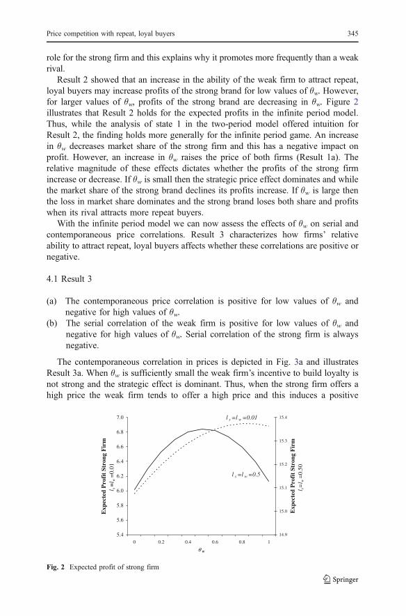
Result 2 showed that an increase in the ability of the weak firm to attract repeat,loyal buyers may increase profits of the strong brand for low values of θw. However,for larger values of θw, profits of the strong brand are decreasing in θw. Figure 2illustrates that Result 2 holds for the expected profits in the infinite period model.Thus, while the analysis of state 1 in the two-period model offered intuition forResult 2, the finding holds more generally for the infinite period game. An increasein θw decreases market share of the strong firm and this has a negative impact onprofit. However, an increase in θw raises the price of both firms (Result 1a). Therelative magnitude of these effects dictates whether the profits of the strong firmincrease or decrease. If θw is small then the strategic price effect dominates and whilethe market share of the strong brand declines its profits increase. If θw is large thenthe loss in market share dominates and the strong brand loses both share and profitswhen its rival attracts more repeat buyers.

With the infinite period model we can now assess the effects of θw on serial andcontemporaneous price correlations. Result 3 characterizes how firms’ relativeability to attract repeat, loyal buyers affects whether these correlations are positive ornegative.

4.1 Result 3

(a) The contemporaneous price correlation is positive for low values of θw andnegative for high values of θw.

(b) The serial correlation of the weak firm is positive for low values of θw andnegative for high values of θw. Serial correlation of the strong firm is alwaysnegative.

The contemporaneous correlation in prices is depicted in Fig. 3a and illustratesResult 3a. When θw is sufficiently small the weak firm’s incentive to build loyalty isnot strong and the strategic effect is dominant. Thus, when the strong firm offers ahigh price the weak firm tends to offer a high price and this induces a positive

5.4

5.6

5.8

6.0

6.2

6.4

6.6

6.8

7.0

0 0.2 0.4 0.6 0.8 1

θ w

Exp

ecte

d P

rofi

t St

rong

Fir

m

l s= l

w=

0.01

14.9

15.0

15.1

15.2

15.3

15.4

Exp

ecte

d P

rofi

t St

rong

Fir

ml s=

l w=

0.50

l s =l w =0.5

l s =l w =0.01

Fig. 2 Expected profit of strong firm


correlation. As θw increases, the direct effect becomes important for both firms andeach uses high-low pricing. In state 0, the strong firm offers high prices to capturemargin on loyal consumers and the weak firm offers low prices to build loyalty. Instate 1, the weak firm offers high prices to capture margin on loyal consumers andthe strong firm offers low prices to build loyalty (see Appendix, Fig. 6). This resultsin a negative contemporaneous price correlation for large values of θw.

The use of high-low pricing also explains Result 3b, which is shown graphicallyin Fig. 3b. The strong firm always uses high-low pricing to build loyalty and thencapture profits, and this leads to negative serial correlation. Unlike the strong firm,the weak firm does not engage in high-low pricing for low values of θw. The mainreason is that in state 0 there is no incentive to offer a low price when θw is low.Instead, the weak firm raises its price in state 0 and this leads to positive serialcorrelation.

A surprising insight from Fig. 3 is that the weak firm may have both positive serialand contemporaneous price correlations for low values of θw. Positive contempora-neous correlation implies that the weak and strong firm follow similar pricingstrategies. Since the strong firm uses high-low pricing, one might predict that the weakfirm would also use high-low pricing. However, the model shows that the weak firm’sserial price correlation is positive for low values of θw. Thus, in a qualitative sense theweak firm probabilistically mimics the strong firm (positive contemporaneouscorrelation). But, the mimicry is not extreme since the serial price correlation is positive.

Result 3b offers an explanation for the variation in competitive price responseshown by Kopalle et al. (1999) in the dishwashing detergent category. The authorsestimate the price response function proposed by Leeflang and Wittink (1992, 1996)for six brands of dishwashing detergent. For the 30 brand pairs, they find eightsignificant negative coefficients and eight significant positive coefficients. Closerinspection reveals that the variation in these competitive response coefficients is

-0.20

-0.15

-0.10

-0.05

0.00

0.05

0.10

0.15

0 0.2 0.4 0.6 0.8 1

θ w

Con

tem

pora

neou

s C

orre

lati

on

l s =l w =0.50

l s =l w =0.01

-0.55

-0.50

-0.45

-0.40

-0.35

-0.30

-0.25

-0.20

-0.15

-0.10

-0.05

0.00

0.05

0.10

0 0.2 0.4 0.6 0.8 1

θ w

Seri

al C

orre

lati

on l s =l w =0.5

l s =l w =0.01

a b

Weak Firm Strong Firm

Fig. 3 Contemporaneous and serial correlation


systematic. To uncover the underlying pattern, we categorize the three largest sharebrands (Dawn, Palmolive, and Sunlight) as strong brands and the three lowest sharebrands (Ivory, C.W. Octagon, and Dove) as weak brands in Table 2.

Negative (positive) coefficients in Table 2 indicate that the temporal correlation ofprice promotions is negative (positive). In other words, a brand is more (less) likelyto promote in the current period if a competing brand promoted last period. Table 2shows that the effect of strong brands on other strong brands is either negative or notsignificant implying alternating retail price promotions.3 For competition betweenweak brands, the effect is mostly insignificant suggesting the timing of promotion tobe independent of competitive action. In contrast, the effect of strong brands onweak brands tends to be positive (4 of 5 cases) or not significant (4 cases). A similarpattern appears for the effect of weak brands on strong brands (4 of 6 positive, 3 notsignificant). This pattern of response coefficients is broadly consistent withpredictions from Result 3b.

Finally, in our model, firms’ pricing strategies incorporate discounted futureprofits. This contrasts with static promotion models (Narasimhan 1988; Raju et al.1990) in which firms optimize current profits. To benchmark our dynamic modelagainst static promotion models, we consider the case where firms ignore futureprofits (δ=0) and the equilibrium pricing strategy for both firms is identical toNarasimhan (1988). To illustrate our results we will focus on the case where firmsare perfectly myopic, δ=0, and compare against our assumed discount factor, δ=0.9.In the dynamic game the continuation payoff is V ¼ p þ dV and to compare profitswith the static game we focus on π, which is the expected current period profit. Theaverage prices in the myopic and dynamic cases are plotted in Fig. 4 and expectedcurrent period profits are plotted in Fig. 5. Our results are summarized as follows.

4.2 Result 4

If firms are perfectly myopic (δ=0), then relative to the dynamic model (δ>0)

(a) The average price of each firm increases if the number of dynamic loyalconsumers is sufficiently large,

(b) Expected current period profits of the weak firm always increases and expectedcurrent period profits of the strong firm increases if the number of dynamicloyal consumers is sufficiently large.

When firms are myopic they ignore the effect of their current pricing strategy onfuture profits. The effect of myopia differs in each state and varies with θw becausethe number of loyal consumers changes. In state 0, a myopic strong firm faces manyloyal consumers, focuses on short-run profits and ignores the possibility of buildingfuture loyal consumers. Lack of concern for future profits raises the average price ofa myopic strong firm in state 0, which in-turn raises the price of a myopic weak firmin state 0. In state 1, two related effects lead to a lower average price in the myopicgame for low values of θw. First, competition for switching consumers lowers bothfirms’ average price and second, the intense price competition increases theoccurrence of state 1. Larger values of θw increase the number of loyal consumers

3 Such an alternating pattern is also noted in Lal (1990) and Kopalle et al. (1999).


in state 1 and this softens price competition in the myopic game. In addition, pricesincrease at a faster rate compared to the dynamic game because firms ignore thepossibility of building future loyal consumers. Eventually myopia leads to higherprices in state 1 compared to the dynamic game.

When θw is low the effects in state 1 dominate and the average price decreases inthe myopic game. That is, the increase in average price in state 0 is outweighed byboth the lower average price in state 1 and the increased occurrence of state 1. As θwincreases there is less price competition in state 1 and a lack of concern for futureprofits leads to higher prices versus the dynamic game.

Our analysis of myopia highlights two marginal effects in the dynamic game thatarise due to a concern for future profits. First, when the market is composed ofprimarily switching consumers there is less price competition, which increases theaverage price. Second, even when firms sell to many loyal consumers there is aconcern for building a future base of loyal consumers. This has a marginal effect oflowering prices in the dynamic game.

Table 2 Price reaction coefficients from Kopalle et al (1999)

Effect on: Effect of:

Strong brands(high share brands) Weak brands(low share brands)

Strong brands (high share brands) 4 negative 2 negative0 positive 4 positive2 not significant 3 not significant

Weak brands (low share brands) 1 negative 1 negative4 positive 0 positive4 not significant 5 not significant

0.1

0.2

0.3

0.4

0.5

0.6

0.7

0.8

0.9

0 0.2 0.4 0.6 0.8 1

θ w

Ex

pected

Pric

e

l =0.50

l=0.01

0.1

0.2

0.3

0.4

0.5

0.6

0.7

0.8

0.9

0 0.2 0.4 0.6 0.8 1

θw

Ex

pected

Pric

e

l =0.5

l =0.01

Myopic Weak Firm Dynamic Weak Firm Myopic Strong Firm Dynamic Strong Firm

Fig. 4 Impact of dynamics on expected price


The impact of myopia on each firm’s profits is shown in Fig. 5 and differs foreach firm. Surprisingly, the weak firm always benefits from myopia. While lowvalues of θw lower the average price of the weak firm, a gain in market sharecompensates for lost margin. In contrast, myopia decreases profits of the strong firmfor low values of θw. As θw increases price competition becomes less intense and thestrong firm benefits from the higher prices induced by myopia.

It is useful to contrast this result with Chintagunta and Rao (1996), who alsoanalyze pricing strategies in a dynamic duopoly. Similar to our model, they find thatmyopic pricing leads to higher expected prices when there is dynamic, consumerloyalty. Chintagunta and Rao (1996) also claim that myopic pricing leads to lowerprofits, which differs from Result 4. This difference can be explained by the relativeimportance of the direct and strategic effects in each model. In both models, myopicfirms fail to recognize the future benefits of building a loyal base of consumers. Thisresults in higher prices and a loss in market share, which is the direct effect. But, inour model the strategic effect outweighs the direct loss in market share when bothfirms attract sufficient numbers of repeat, loyal buyers. The reason for this differenceis that Chintagunta and Rao (1996) focus on long-run, steady state pricing strategies.Consumer dynamics plays a role in the evolution of pricing strategies but does notplay a role in steady-state. In contrast, consumer dynamics always plays a role in ourmodel since consumers continually enter and exit the market.

5 Discussion and conclusions

Many empirical studies have established that state dependence varies acrossconsumers, brands, and categories. Previous analytic models have assumed thatstate dependence is a customer characteristic that does not vary across firms. Incontrast, we take the view that state dependence varies by firm. That is, a well-

0.1

0.2

0.3

0.4

0.5

0.6

0.7

0.8

0.9

0 0.2 0.4 0.6 0.8 1

Exp

ecte

d P

rofi

t

Dynamic Weak Firm Dynamic Strong Firm

Myopic Weak Firm Myopic Strong Firm

θ w

Fig. 5 Impact of dynamics onexpected profit


known national brand, such as Tide detergent, may be able to attract more repeat,loyal buyers than a lesser-known rival brand. While this view of state dependence issupported by empirical research (Van Oest and Frances 2003), it has not beenpreviously considered in analytic models.

Importantly, we show a firm’s relative ability to attract repeat, loyal buyers hassurprising implications for firms’ pricing strategies. We show that this single effectcan explain why leading brands such Parkay and Peter Pan may offer both the lowestaverage price and the most frequent promotions. For managers, this result shows thatfrequent, deep promotions may be optimal to maintaining a dominant marketposition. In this sense, we identify an alternative pricing strategy that a managershould consider to build and maintain a leading brand. While a strategy of low pricesand frequent promotions is not always profitable, our model identifies conditionsunder which this strategy is optimal.

We also find that profits of a firm may increase when a weak competitor is able toattract more repeat, loyal buyers. This shows that if a firm becomes weaker it maylower the price of all firms and erode industry profits. An implication for managersis that a leading brand must be cautious using tactics that weaken a rival as this maylead to the unexpected consequence of lower industry prices and profits for bothfirms.

Our findings on price correlations complement extant theoretical research on pricepromotions and price cycles. Consistent with this literature, we show that strongfirms exhibit high-low pricing or negative serial price correlation. However, strategicprice effects may lead a weak competitor to mimic the behavior of the strong firm,which may lead to both positive serial and contemporaneous price correlations. Wenote that these findings are entirely due to competitive effects; in the absence ofcompetition, a weak firm would exhibit negative serial price correlation. Forpractitioners, these results show when it is optimal for a weaker brand to mimic astronger rival’s pricing strategy. If the firms are sufficiently asymmetric in theirability to attract repeat, loyal buyers then mimicry of the competitor’s pricing strategyis optimal.

A limitation of the infinite period model is that we allow consumers to live foronly two periods. We maintain this assumption for tractability but this assumptiondoes not drive our results. To illustrate this point, we extend the model to a threeperiod overlapping generations model (see Appendix). All of our results hold in thethree period OLG model, which illustrates that the assumption is not restrictive.

An additional limitation of our model is that we do not allow for strategic consumerbehavior. That is, a strategic consumer may forgo a low price today if the consumeranticipates becoming loyal and paying a high price tomorrow. Incorporating strategicbehavior is clearly important (Villas-Boas 2004a, b, 2006), but is not feasible in thismodel structure. However, we can show that for low values of θw and l consumerbehavior is dynamically consistent in our model. This suggests that our results willextend to a game with strategic consumer behavior, which is an area of future research.

This paper incorporates consumer dynamics that are well-established in empiricalmarketing studies. The model allows us to highlight how firms’ ability to attractrepeat, loyal buyers affects pricing strategies and profits. Reassuringly, there isconsistency between model predictions and extant empirical findings, but additionalempirical research is required to formally test these predictions.


Appendix

Two-period model

Proof of Result 1

Proof:

(a) In period 2 state 0 both firms charge r. In state 1, the weak brand has a pointmass at r and both firms randomize in the interval ½p21; r�.

Note that: Fs21 pð Þ � Fw21 pð Þ ¼ θw p 1þlð Þ�r lþθwð Þð Þp 1þlð Þ 1�θwð Þ > 0. This implies that Fw21( p)

first-order stochastically dominates Fs21( p) so that the expected price charged by theweak brand in state 1 is greater than that charged by the strong brand. In period 1,once again the weak brand has a point mass at r and both firms randomize in theinterval ½p1; r�.

Fs1 pð Þ � Fw1 pð Þ ¼ rδ 1þ l � θwð Þ 1� θwð Þ p� l r � pð Þ þ rδθwð Þpþ rδθwð Þ p 1þ lð Þ þ rδ 1þ l � 1� θwð Þθwð Þð Þ > 0

Given that Fw1( p) first-order stochastically dominates Fs1( p) the expected pricecharged by the weak brand in period 1 is greater than that charged by the strongbrand. Together this implies that the expected price of the strong brand is less thanthe weak brand.(b) In period 2 state 0 neither firm promotes. In state 1, the weak brand has a point

mass at r and hence the strong brand promotes more frequently in state 1. Inperiod 1 the weak brand has a point mass at r so once again the strong brandpromotes more frequently.

Result 2

The expected profits in state 1 of the strong firm are increasing for low values of θwand decreasing for large values of θw.

Proof: πs21 ¼ p21ðl þ ð1� θwÞÞ ¼rðlþθwÞlþ1ð Þ ðl þ ð1� θwÞÞ

@πs21

@θw¼ r

l þ 1ð Þ 1� 2θwð Þ�> 0; θw < 1=2� 0; θw � 1=2

Solutions for infinite horizon model

Let Vc*jk and pc*k be the equilibrium solution for firm j in state k for case c. Define

pw0, ps0, pw1 and ps1 as the solution to:

r2lw þ δVw0 ¼ pw0 2lw þ 2� θsð Þ þ δVw1 ð20Þ


r 2ls þ θsð Þ þ δVs1 ¼ ps0 2ls þ 2ð Þ þ δVs0 ð21Þ

r 2lw þ θwð Þ þ δVw0 ¼ pw1 2lw þ 2ð Þ þ δVw1 ð22Þ

r2ls þ δVs1 ¼ ps1 2ls þ 2� θwð Þ þ δVs0 ð23Þ

Case 1

In this case Fw0 rð Þ ¼ 1 and Fs1 rð Þ ¼ 1. Case 1 is feasible if ps1 < p1*1 andpw0 < p1*0 , which is equivalent to conditions C1 and C2, respectively.

V 1*w0 ¼ r 2lw þ θwð Þ

δ 1� δ2� � þ

r 2lw þ 2� θsð Þ4δlw þ 4ls 1þ lw þ δ 1þ 2lwð Þð Þþ2 1þ lwð Þ 1þ δð Þθsþ2δθw 1þ ls � lwð Þ � δθ2w

0@

1A

0@

1A

1� δ2� � 2 1þ lsð Þ 2þ lw 2þ 4δð Þ þ δ 4þ δθsð Þð Þ

þδ2 2lw þ 2� θsð Þθw

0BBBBBB@

1CCCCCCA

ð24Þ

V 1*w1 ¼

2 1þ lwð Þr δ 2� θsð Þ 2ls þ θsð Þ þ 2lw 2þ ls 2þ 4δð Þ þ δ 2þ θsð Þð Þþ2 1þ lsð Þ 1þ δð Þθw

1� δð Þ 2 1þ lsð Þ 2þ 2lw 1þ 2δð Þ þ δ 4þ δθsð Þð Þ þ δ2 2lw þ 2� θsð Þθw

� �� ð25Þ

V 1*s0 ¼

2 1þ lsð Þ 2r 1þ lwð Þ 1� δ2� �

2ls þ θsð Þþrδ 1� δð Þ 2ls þ 2� θwð Þ 2lw þ θwð Þ

4 1þ lsð Þ 1þ lwð Þ 1� δ2� �2 � δ2 1� δð Þ2 2lw þ 2� θsð Þ 2ls þ 2� θwð Þ

� �ð26Þ

V 1*s1 ¼ 1

δ

2 1þ lsð Þ 2r 1þ lwð Þ 1þ δð Þ 2ls þ θsð Þþrδ 2ls þ 2� θwð Þ 2lw þ θwð Þ

4 1þ lsð Þ 1þ lwð Þ 1þ δð Þ2 1� δð Þ�δ2 1þ δð Þ 2lw þ 2� θsð Þ 2ls þ 2� θwð Þ

� r 2ls þ θsð Þ

0BB@

1CCA ð27Þ

p1*0 ¼ r 4lwδ þ 4ls 1þ lw þ δ þ 2lwδð Þ þ 2θs 1þ lwð Þ 1þ δð Þ þ 2δθw 1þ ls � lwð Þ � δθ2w� ��

2 1þ lsð Þ 2þ 2lw 1þ 2δð Þ þ δ 4þ δθsð Þð Þ þ δ2θw 2lw þ 2� θsð Þ� � ð28Þ

p1*1 ¼ r 4lw 1þ ls þ δ þ 2lsδð Þ þ 2δlwθs þ δ 2� θsð Þ 2ls þ θsð Þ þ 2θw 1þ lsð Þ 1þ δð Þð Þð Þ2 1þ lsð Þ 2þ 2lw 1þ 2δð Þ þ δ 4þ δθsð Þð Þ þ δ2θw 2lw þ 2� θsð Þ� � ð29Þ(29)


C1 :

r2 1þ lsð Þ δθs 4� θs 1� δð Þð Þ � 4lw 1þ δθsð Þ þ 2ls 2þ δθsð Þð Þ

þ 4þ 4l2s � 4lw þ 4ls 2� lw � δ 1þ lwð Þð Þþ2lsδθs � 1� δð Þδ 2þ 2lw � θsð Þθs

θw � 2 1þ lsð Þθ2w

0@

1A

0@

1A

2þ 2ls � θwð Þ 2 1þ lsð Þ 2þ lw 2þ 4δð Þ þ δ 4þ δθsð Þð Þ þ δ2 2þ 2lw � θsð Þθw� �� > 0

C2 :

r8 1þ lwð Þ ls � lwð Þ þ 4 1� ls þ lwð Þ 1þ lwð Þ � 1þ lsð Þlwδð Þθs � 2 1þ lwð Þθ2sþ2δ 2 2þ 2ls � lwð Þ 1þ lwð Þ � 1� lw þ ls 1� δð Þ � δð Þθsð Þθw�δ 1� δð Þ 2þ 2lw � θsð Þθ2w

0@

1A

0@

1A

2þ 2lw � θsð Þ 2 1þ lsð Þ 2þ lw 2þ 4δð Þ þ δ 4þ δθsð Þð Þ þ δ2 2þ 2lw � θsð Þθw� �� > 0

Case 2

In this case Fw0 rð Þ ¼ 1 and Fw1 rð Þ ¼ 1. Case 2 is feasible if pw1 < p2*1 and pw0 < p2*0or equivalently if conditions C3 and C4 hold.

V 2*w0 ¼ r 2lw þ 2� θsð Þð Þ 2ls þ θs 1� δð Þð Þ

2 1þ lsð Þ þ 2rδ 1þ lwð Þ 2ls � δθsð Þ1� δð Þ 2lw þ 2� θwð Þð Þ ð30Þ

V 2*w1 ¼ 2r 1þ lwð Þ 2ls � δθsð Þ

1� δð Þ 2lw þ 2� θwð Þð Þ ð31Þ

V 2*s0 ¼ r

2ls1� δ

þ θs

ð32Þ

V 2*s1 ¼ r

2ls1� δ

ð33Þ

p2*0 ¼ r 2ls þ θs 1� δð Þð Þ2 1þ lsð Þ ð34Þ

p2*1 ¼ r 2ls � δθsð Þ2ls þ 2� θwð Þ ð35Þ

Substituting Eqs. 30–35 in the conditions pw1 < p2*1 and pw0 < p2*0 we obtain thefollowing two conditions:

C3 :

2r 1þ lsð Þ 4 ls � lwð Þ þ 2 1þ lw � ls 1� δð Þ � 2 1þ lwð Þδð Þθs � 1� δð Þ2θ2s� �

þr 4 lw � ls 1� δ � lwδð Þð Þ þ 2 ls � 1þ lwð Þ 1� δð Þð Þ 1� δð Þθs þ 1� δð Þ2θ2s� �

θw

0@

1A

2 1þ lsð Þ 2þ 2lw � θsð Þ 2þ 2ls � θwð Þð Þ > 0 ð36Þ


C4 :

r

2 1þ lsð Þ 2ls 2þ δθsð Þ � δθs 4� θs þ δθsð Þ � 4lw 1þ δθsð Þð Þ�4þ 4l2s � 4lw þ 4ls 2� lw � δ 1þ lwð Þð Þþ2lsδθs � δ 1� δð Þ 2þ 2lw � θsð Þθs

!θw

þ2 1þ lsð Þθ2w

0BBBB@

1CCCCA

0BBBB@

1CCCCA

4 1þ lsð Þ 1þ lwð Þ 2þ 2ls � θwð Þð Þ > 0 ð37Þ

Case 3

In this case Fs0 rð Þ ¼ 1 and Fw1 rð Þ ¼ 1. Case 3 is feasible if pw1 < p3*1 and ps0 < p3*0or equivalently if conditions C5 and C6 hold.

V 3*w0 ¼ 2lwr

1� δð38Þ

V 3*w1 ¼ 4 1þ lwð Þr 1� δð Þ 2 1þ lsð Þlwδ � ls 1� δð Þ 2þ 2lw � θsð Þð Þð Þ

1� δð Þ2 4 1þ lsð Þ 1þ lwð Þδ2 � 1� δð Þ2 2lw þ 2� θsð Þ 2ls þ 2� θwð Þ� �� ð39Þ

V 3*s0 ¼ 4 1þ lsð Þr 2 1þ lsð Þlw � 2 ls þ lw þ 2lslwð Þδ � lw 1� δð Þθwð Þð Þ

2 1þ lsð Þ 2 1þ lwð Þ 1� δð Þ 1� 2δð Þ � 1� δð Þ3θs� �

� 1� δð Þ3 2þ 2lw � θsð Þθw� � ð40Þ

V 3*s1 ¼ 2lsr

1� δð41Þ

p3*0 ¼ 2r 2lsδ � lw ls 2� 4δð Þ þ 1� δð Þ 2� θwð Þð Þð Þð Þ2 1þ lsð Þ 2 1þ lwð Þ 2δ � 1ð Þ þ 1� δð Þ2θs

� �þ 1� δð Þ2 2lw þ 2� θsð Þθw

� �ð42Þ

p3*1 ¼ 2r 2lwδ þ ls lw 2� 4δð Þ þ 1� δð Þ 2� θsð Þð Þð Þð Þ2 1þ lsð Þ 2 1þ lwð Þ 2δ � 1ð Þ þ 1� δð Þ2θs

� �þ 1� δð Þ2 2lw þ 2� θsð Þθw

� �ð43Þ

Substituting Eqs. 38–43 in the conditions pw1 < p3*1 and ps0 < p3*0 we obtain thefollowing conditions:

C5 :

2 1þ lsð Þr 4 ls � lwð Þ þ 2 1þ lw � ls 1� δð Þ � 2 1þ lwð Þδð Þθs � 1� δð Þ2θ2s� �

þr 4 lw � ls 1� δ 1þ lwð Þð Þð Þ þ 2 ls � 1� δð Þ 1þ lwð Þð Þ 1� δð Þθs � 1� δð Þ2θ2s� �

θw

0BBB@

1CCCA

2 1þ lsð Þ 2 1þ lsð Þ 2 1þ lwð Þ 2δ � 1ð Þ þ 1� δð Þ2θs� �

þ 1� δð Þ2 2þ 2lw � θsð Þθw� �� > 0

ð44Þ


C6 :

r

8 lw � lsð Þ 1þ lwð Þ þ 4 ls � lw 1� δð Þ þ lslwδð Þθs

þ22 1þ lwð Þ 1þ ls � lw 1� δð Þ � 2δ 1þ lsð Þð Þþ 1� δð Þ 1� lw � ls 1� δð Þ þ δð Þθs

θw

� 1� δð Þ2 2þ 2lw � θsð Þθ2w

0BBBB@

1CCCCA

0BBBB@

1CCCCA

2 1þ lwð Þ 2 1þ lsð Þ 2 1þ lwð Þ 2δ � 1ð Þ þ 1� δð Þ2θs� �

þ 1� δð Þ2 2þ 2lw � θsð Þθw� �� > 0

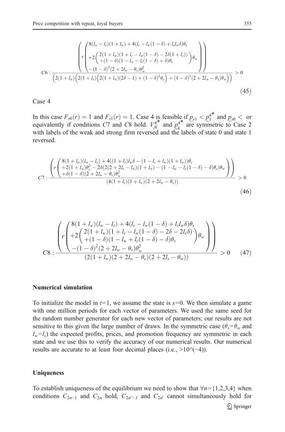
ð45ÞCase 4

In this case Fs0 rð Þ ¼ 1 and Fs1 rð Þ ¼ 1. Case 4 is feasible if ps1 < p4*1 and ps0 < orequivalently if conditions C7 and C8 hold. V 4*

jk and p4*k

are symmetric to Case 2with labels of the weak and strong firm reversed and the labels of state 0 and state 1reversed.

C7 :

r8 1þ lwð Þ lw � lsð Þ þ 4 1þ lsð Þlwδ � 1� ls þ lwð Þ 1þ lwð Þð Þθsþ2 1þ lwð Þθ2s � 2δ 2 2þ 2ls � lwð Þ 1þ lwð Þ � 1� lw � ls 1� δð Þ � δð Þθsð Þθwþδ 1� δð Þ 2þ 2lw � θsð Þθ2w

0@

1A

0@

1A

4 1þ lsð Þ 1þ lwð Þ 2þ 2lw � θsð Þð Þ > 0

ð46Þ

C8 :

r

8 1þ lwð Þ lw � lsð Þ þ 4 ls � lw 1� δð Þ þ lslwδð Þθsþ2

2 1þ lwð Þ 1þ ls � lw 1� δð Þ � 2δ � 2lsδð Þþ 1� δð Þ 1� lw þ ls 1� δð Þ � δð Þθs

θw

� 1� δð Þ2 2þ 2lw � θsð Þθ2w

0BB@

1CCA

0BB@

1CCA

2 1þ lwð Þ 2þ 2lw � θsð Þ 2þ 2ls � θwð Þð Þ > 0 ð47Þ

Numerical simulation

To initialize the model in t=1, we assume the state is s=0. We then simulate a gamewith one million periods for each vector of parameters. We used the same seed forthe random number generator for each new vector of parameters; our results are notsensitive to this given the large number of draws. In the symmetric case (θs=θw andlw= ls) the expected profits, prices, and promotion frequency are symmetric in eachstate and we use this to verify the accuracy of our numerical results. Our numericalresults are accurate to at least four decimal places (i.e., >10^(−4)).

Uniqueness

To establish uniqueness of the equilibrium we need to show that ∀n={1,2,3,4} whenconditions C2n−1 and C2n hold, C2n0−1 and C2n0 cannot simultaneously hold for


8n0 6¼ n ¼ 1; 2; 3; 4f g. Because of the complexity of the expressions we are unableto analytically establish uniqueness but we are able to confirm uniqueness withextensive numerical simulations (available from authors). As an example, considerthe following parameters values: {r=1, δ=0.9, θs=1, lw=0.01, ls=0.01}. Evaluatingconditions C1–C8 at these parameter values we obtain expressions for theseconditions which are a function only of θw. Evaluated at these parameter values wefind the following:

C1 > 0; 8θw 2 0; 2:02½ Þ [ 3:09;1ð � and C1 < 0; 8θw 2 2:02; 3:09ð ÞC2 > 0; 8θw 2 0; 78:10½ Þ and C2 < 0; 8θw 2 78:10;1ð �C3 < 0; 8θw 2 0; 2:02½ Þ and C3 > 0; 8θw > 2:02

C4 < 0; 8θw 2 0; 2:02½ Þ [ 3:09;1ð � and C4 > 0; θw 2 2:02; 3:09ð ÞC5 < 0; 8θw < 116:78 and C5 > 0; 8θw > 116:78

C6 > 0; 8θw 2 0; 0:011½ Þ and C6 < 0; 8θw > 0:011

C7 < 0; 8θw 2 0; 78:10½ Þ and C7 > 0; 8θw > 78:10

C8 < 0; 8θw < 2:02 and C8 > 0;8θw > 2:02

Table 3 specifies the unique equilibrium for different values of θw. For each rangeboth conditions for a single case are satisfied and at least one condition for theremaining cases is not satisfied. This proves uniqueness. As an example, forθw∈[0,2.02) conditions C1>0 and C2>0, which proves that Case 1 is an equilibrium.In this range the other cases are not feasible (C3<0, C5<0, and C7<0), whichproves that Case 1 is a unique equilibrium.

Additional results

Figure 6 further illustrates the average price offered by each firm in each state. Inparticular, the figure shows that for low values of θw the weak firm offers a higherprice in state 0 than in state 1.

Model extension

To demonstrate the robustness of our model we analyze a game in which consumerslive for three periods rather than two periods. This results in four possible states that

Parameter region Equilibrium

θw∈[0, 2.02) Case 1θw∈(2.02, 3.09) Case 2θw∈(3.09, 78.10) Case 1θw∈(78.10, ∞) Case 4

Table 3 Uniqueness: anillustration


we label k=0, 1, 2, and 3. In state 0 there are 2θs dynamic loyal consumers for thestrong firm and zero for the weak firm. In state 3 there are 2θw dynamic loyalconsumers for the weak firm and zero for the strong firm. In states 1 and 2 there areθs + θw dynamic loyal consumers who live for one or two additional periods. Werefer to a consumer as “old” if they have one period remaining and “young” if theyhave two periods remaining. In state 1, there are θs old consumers and θw youngconsumers. In state 2, there are θs young consumers and θw old consumers.

The analysis of the model is analogous to Section 2 and details are available fromthe authors. We specify eight continuation payoffs and then solve for eight CDFs (2

0.10

0.20

0.30

0.40

0.50

0.60

0.70

0.80

0.90

0.00 0.20 0.40 0.60 0.80 1.00θ w

Exp

ecte

d P

rice

Weak Firm State 0 Strong Firm State 0


Fig. 6 Expected price in each state for l=0.01

0.00

0.10

0.20

0.30

0.40

0.50

0.60

0.70

0.80

0.90

0.00 0.20 0.40 0.60 0.80 1.00θ w

Exp

ecte

d P

rice



0.00

0.10

0.20

0.30

0.40

0.50

0.60

0.70

0.80

0.90

0.00 0.20 0.40 0.60 0.80 1.00

θ w

Exp

ecte

d P

rice



a b

Fig. 7 Expected price in each state for 3 period OLG game


firms × 4 states) as a function of Vjk and pk . The 12 equilibrium values for V*jk andp*k require 12 equations and eight of these are given by FjkðpkÞ ¼ 0. There are fourpossible states and in each state exactly one firm has a mass point, which leads to 16(42) possible solutions. In our simulations, we focus on a solution analogous to Case1 where the strong firm has a mass point in states 0 and 2 and the weak firm has amass point in states 1 and 3. In each of these states, the firm with the mass pointoffered the lowest price in the previous period and hence acquired a new group ofdynamic loyal consumers.

Analysis of this model, which is available from the authors, demonstrates that ourresults hold in a richer, more complex model. The assumption that consumers livefor two periods yields a parsimonious model and our results continue to hold whenconsumers live for more than two periods. To illustrate the similarity of the models,we plot the expected price in Fig. 7. In Fig. 7a we consider the two extreme states(state 0 and 3) where one firm has 2θj dynamic loyal consumers and the other firmhas zero. Given the similarity of Figs. 6 and 7a, it is not surprising that our resultshold in the three period OLG model. In Fig. 7b, we analyze the intermediate stateswhere each firm has θj dynamic loyal consumers. We find that firms offer low priceswhen they have θj young loyal consumers and zero old loyal consumers to buildtheir loyal base of consumers. If successful at acquiring switching consumers, firmsthen transition to the state where they have 2θj dynamic loyal consumers. At thispoint, they “harvest” and offer high prices to their loyal consumers.

In contrast, when a firm has zero young loyal consumers and θj old loyalconsumers should it offer high prices (“harvest”) or offer low prices (“invest”)? Wefind that the strong firm’s expected price is higher in state 1 (θs old loyal consumers)compared to state 2 (zero old loyal consumers). Similarly, the weak firm offershigher prices in state 2 (θw old loyal consumers) compared to state 1 (zero old loyalconsumers). This indicates that the incentive to harvest old loyal consumersdominates the incentive to build a loyal base of consumers.

Overall, the extension demonstrates the robustness of our results. It also suggeststhat firms will offer high prices in multiple periods to extract profits on their loyalbase of consumers. When the loyal base of consumers is sufficiently low, the firmwill offer a series of deep promotions to establish a loyal base of consumers. Oncethe loyal base of consumers is established the cycle repeats.

References

Anderson, E. T., Kumar, N., & Rajiv, S. (2004). A comment on: Revisiting dynamic duopoly withconsumer switching costs. Journal of Economic Theory, 116(1), 177–186.

Anderson, E. T., & Simester, D. (2004). Long-run effects of promotion depth on new versus establishedcustomers: Three field studies. Marketing Science, 23(1), 4–20.

Beggs, A., & Klemperer, P. (1992). Multi-period competition with switching costs. Econometrica, 60(3), 651–666.Chintagunta, P., & Rao, V. (1996). Pricing strategies in a dynamic duopoly: A differential game model.

Management Science, 42(11), 1501–1514.Conlisk, J., Gerstner, E., & Sobel, J. (1984). Cyclic pricing by a durable goods monopolist. Quarterly

Journal of Economics, 99(3), 489–505.Erdem, T., & Keane, M. P. (1996). Decision-making under uncertainty: Capturing dynamic brand choice

processes in turbulent consumer goods markets. Marketing Science, 15(1), 1–20.


Foekens, E. W., Leeflang, P. S. H., & Wittink, D. R. (1999). Varying parameter models to accommodatedynamic promotion effects. Journal of Econometrics, 89(2), 249–268.

Guadagni, P. M., & Little, J. D. C. (1983). A logit model of brand choice calibrated on scanner data.Marketing Science, 1(2), 203–238.

Klemperer, P. (1995). Competition when consumers have switching costs: An overview with applications toindustrial organization, macroeconomics, and international trade. Review of Economic Studies, 62(4),515–539.

Klemperer, P. (1987a). Markets with consumer switching costs. Quarterly Journal of Economics, 102(2),375–394.

Klemperer, P. (1987b). Entry deterrence in markets with consumer switching costs. Economic Journal, 97(0), 99–117.

Klemperer, P. (1989). Price wars caused by switching costs. The Review of Economic Studies, 56(3), 405–420.Kopalle, P. K., Mela, C., & Marsh, L. (1999). The dynamic effect of discounting on sales: Empirical

analysis and normative pricing implications. Marketing Science, 18(3), 317–332.Lal, R. (1990). Price promotions: Limiting competitive encroachment. Marketing Science, 9(3), 247–262.Leeflang, P. S. H., & Wittink, D. R. (1992). Diagnosing competitive reactions using (aggregated) scanner

data. International Journal of Research in Marketing, 9(1), 39–57.Leeflang, P. S. H., & Wittink, D. R. (1996). Competitive reaction versus consumer response: Do managers

overreact? International Journal of Research in Marketing, 13(2), 103–119.Mela, C., Gupta, S., & Lehmann, D. (1997). The long-term effect of promotion and advertising on

consumer brand choice. Journal of Marketing Research, 34(2), 246–261.Narasimhan, C. (1988). Competitive promotional strategies. Journal of Business, 61(4), 427–449.Padilla, A. J. (1995). Revisiting dynamic duopoly with consumer switching costs. Journal of Economic

Theory, 67(2), 520–530.Raju, J. S., Srinivasan, V., & Lal, R. (1990). Effectiveness of brand loyalty on competitive price

promotional strategies. Management Science, 36(3), 276–304.Rao, R. C. (1991). Pricing and promotions in asymmetric duopolies. Marketing Science, 10(2), 131–144.Seetharaman, P. B., Ainslie, A., & Chintagunta, P. K. (1999). Investigating household state dependence

effects across categories. Journal of Marketing Research, 36(4), 488–500.Shilony, Y. (1977). Mixed pricing in an oligopoly. Journal of Economic Theory, 14, 373–388, (April 1977).Sobel, J. (1984). The timing of sales. Review of Economic Studies, 51(3), 353–368.Van Oest, R., & Frances, P. H. (2003). Which brand gains share from which brands? Inference from store-

level scanner data. Tinbergen Institute Discussion Paper.Varian, H. (1980). A model of sales. American Economic Review, 70(4), 651–659.Villas-Boas, J. M. (2004a). Consumer learning, brand loyalty and competition. Marketing Science, 23(1),

134–145.Villas-Boas, J. M. (2004b). Price cycles in markets with customer recognition. Rand Journal of Economics, 35

(3), 486–501.Villas-Boas, J. M. (2006). Dynamic competition with experience goods. Journal of Economics

Management & Strategy, 15(1), 37–66.


price competition with repeat, loyal buyers · price competition with repeat, loyal buyers ......

Documents