pressure drop profiles evaluation with dense gas in a …

IV Journeys in Multiphase Flows (JEM 2017) March27-31, 2017, São Paulo, SP, Brazil

Copyright © 2017 by ABCM Paper ID: JEM-2017-0033

PRESSURE DROP PROFILES EVALUATION WITH DENSE GAS IN A GAS-LIQUID FLOW THROUGH A PIPELINE

Guilherme Rosário dos Santos Petroleum Engineering – Petróleo Brasileiro SA-Marques de Herval Street, 90 – 13rd floor - ZIP CODE: 11010-310, Valongo, Santos-SP [email protected] Mariana Ricken Barbosa Mechanical Engineering Faculty- Campinas State University-Mendeleyv Street, 200- ZIP CODE: 13083-860, Cidade Universitária “Zeferino Vaz” Barão Geraldo-Campinas-SP [email protected] Ricardo Augusto Mazza Mechanical Engineering Faculty- Campinas State University-Mendeleyv Street, 200- ZIP CODE: 13083-860, Cidade Universitária “Zeferino Vaz” Barão Geraldo-Campinas-SP [email protected] Abstract. The production development in the Pre Salt presents several challenges to overcome such as long distances from the coast, deep reservoirs with low temperatures, high-pressure levels, deep water and others. This article aims to study the gas density influence in the pressure drop through a pipeline. To study this, a multiphase model at Olga simulator (two fluid model) was developed, using a R 410 refrigerant mixture as fluid. The fluid properties were generated through PVT Sim software, being R410 refrigerant modeled from its pure components: R-32 and R-125. A flow rate range was evaluated varying downstream pressure for each temperature initial conditions. Besides, it was evaluated the following profiles: gravitational pressure gradient, mean density, liquid and gas densities, liquid superficial velocity and total superficial velocity ratio and void fraction. As it was expected, a higher gas density implies an increasing of mean density, which in turns, implies an increasing of gravitational pressure gradient. In this work, there were not significant changes in liquid densities, being an increasing of gas density the main factor of gravitational pressure gradient increasing. The cases studies point out no significant release of gas which imply low velocities (low frictional pressure gradients). These simulations present consistent results with that were expected. Keywords: dense gas, multiphase flow, pressure drop

1. INTRODUCTION

The production development in the Pre Salt presents several challenges to overcome such as long distances from the coast, deep reservoirs with low temperatures, high-pressure levels, deep water and others. The knowledge of pressure drop profiles are essential to find out problems related to the flow assurance such as wax, inorganic salt, asphaltene depositions and hydrates plugging. In other words, knowledge of profile pressure and its flow rates can be an important tool in order to detect eventual problems that are taking place in the wells, flowline and risers. Figure 1 shows a flow schematic with a well, flowline and riser (Santos and Loureiro, 2012).

Figure 1. Flow Schematic from well to the plataform (Source: Santos and Loureiro, 2012)

Guilherme Santos, Mariana Barbosa and Ricardo Mazza Pressure Drop Profiles Evaluation with Dense Gas in a Gas-Liquid Flow through a Pipeline

On the other hand, a good knowledge of pressure profiles behavior can provide a good accuracy mass flow that can

be produced from wells. For gas injection wells, the knowledge of pressure profiles is also important. It provides a way to inject without exceed fracture pressure. At the same time, pressure downhole (at the bottom well) must be higher than the reservoir pressure in order to take place it. This injection will be more important in a gas network with gas pipeline and injection wells.

One of the most important parameters is the ratio liquid and gas density as well as viscosities ratio and surface stress ratio (Ishikawa et al, 2014). This article aims to study the gas density influence in the pressure drop through a pipeline. To study this, a multiphase model was developed at Olga simulator, using a R 410 refrigerant mixture as fluid. The fluid properties were generated through PVT Sim software, being R410 refrigerant modeled from equimolar quantities of R-32 and R-125. The Olga simulator uses these fluid properties to evaluate profiles in the two phase flow model application. 2. FLUID PROPERTIES SIMULATIONS

In this work, fluid properties simulations were performed through PVT Software (Calsep, 2013). The software output are the fluid properties table that will be used in Olga Simulator. The fluid used was R-410 refrigerant, which was generated from its pure components: equimolar quantities of R-32 and R-125. Table 1 shows fluid properties required of pure components to generate R410 fluid properties:

Table 1. Fluid Properties of R410 Components (Calsep, 2013)

Property R-32 R-125

MW (kg/kmol) 52,0 120,0

ρ l (kg/m3) 1002,6 1251,5

Tc ( C ) 78,1 66,0

Pc (MPa) 5,9 3,7

Vc (m3/mol) 1,23E-05 2,09E-05

w 0,28 0,31

Tb ( C ) -51,7 -48,5

Pb (MPa) 1,5 1,2

Href (J/mol) 28054,5 41098,5

Ai 12,3 11,7

Bi -7,0E-02 2,2E-02

Ci 3,9E-04 8,7E-05

Di -8,4E-07 -1,1E-07

Ei 8,6E-10 0

Fi 0 0

Tf ( C ) -137,0 -103,0

Hf (J/mol) 4400,0 2250,0

Component

wherein MW, ρl, Tc, Pc, Vc, w, Tb, Pb, Href, Tf, Hf are the molecular weight, liquid density at 15oC and atmospheric pressure, temperature, pressure, molar volume in the critical point, acentric factor, boiling point temperature at atmospheric pressure, vapor pressure at 20 oC, ideal gas enthalpy at 20 oC, four coefficients in ideal gas heat capacity polynomial, melting temperature, molar melting enthalpy, respectively.

The phase equilibrium calculation in PVT Sim is based on state equations. Soave-Redich Kwong equation fitted phase

equilibrium, providing pressure as a function of temperature behavior. Three flash vaporization were performed in order to check R-410 properties calculated through this state equation at 0.1 MPa and 20 oC, 2 MPa and 15 oC and 4.126 MPa and 71.34 oC (critical point). The gas heat capacity at 0.1 MPa and 20 oC was 57.62 J/moloC whereas the value found in the literature was 58.42 J/moloC. The liquid density at 2 MPa and 15 oC was 1093.1 kg/m3whereas the value found in the literature was1188 kg/m3. The critical volume was 0.1548 m3/kmol whereas the value found in the literature was 0.1485 m3/kmol (DuPont, 2004). Figure 2 shows R-410 diagram simulated from PVT Sim:

IV Journeys in Multiphase Flows (JEM 2017)

Figure 2. R410 Diagram

3. FLOWS SIMULATIONS

Two types of flow simulations were carried out. The first part aims to compare literature data of pressure drop with the Olga response. In the second part, it can be found the pressure drop prediction from Olga simulator for three different liquid and gas density ratio and temperature.

3.1 Olga comparison with literature data

Several simulations were performed with air water flow, which can be found in the literature. Table 2, Table 3 and

Table 4 show the total gradient pressure results for dispersed bubble, slug and annular patterns, respectively:


Table 2. Total pressure gradient for dispersed bubble flow

Table 3. Total pressure gradient for slug flow

Run Jg (m/s) Jl (m/s) ρl (kg/m3) ρg (kg/m

3) ml (kg/s) mg (kg/s)

∆P/L

measured

(kPa/m)

Poutlet

(kPa)

∆P/L

simulated

(kPa/m)

Relative

Deviation

(%)

1 0,123 0,6 1000 1,25 0,32 8,19E-05 9,6 107,3 8,8 8%

2 0,196 0,6 1000 1,24 0,32 1,29E-04 8,9 106,0 8,3 7%

3 0,214 1,18 1000 1,03 0,63 1,17E-04 9,8 88,3 9,5 3%

4 0,281 2,16 1000 0,98 1,15 1,46E-04 11,0 83,9 11,2 -2%

5 0,189 2,2 1000 0,94 1,17 9,39E-05 11,3 80,1 11,4 -1%

6 0,262 0,9 1000 1,26 0,48 1,76E-04 8,1 108,2 8,6 -7%

7 0,246 1,18 1000 1,30 0,63 1,70E-04 8,8 111,3 9,3 -6%

8 0,450 1,24 1000 1,35 0,66 3,22E-04 8,6 115,4 8,7 -1%

9 0,143 0,29 1000 1,24 0,15 9,38E-05 8,3 105,7 7,8 7%

10 0,132 0,6 1000 1,25 0,32 8,78E-05 9,1 107,2 8,8 4%

11 0,213 0,61 1000 1,24 0,32 1,40E-04 8,5 106,3 8,2 4%

12 0,209 1,19 1000 1,27 0,63 1,41E-04 9,7 108,5 9,5 2%

13 0,130 1,21 1000 1,27 0,64 8,79E-05 10,0 109,0 9,8 2%

14 0,515 2,12 1000 1,29 1,13 3,52E-04 10,6 110,1 10,8 -2%

15 0,264 2,16 1000 1,17 1,15 1,64E-04 11,1 100,3 11,2 -1%

16 0,152 2,22 1000 1,02 1,18 8,22E-05 11,4 87,2 11,5 -1%

17 3,038 2,86 1000 1,50 1,52 2,41E-03 12,0 128,1 12,4 -4%

18 1,716 2,92 1000 1,42 1,55 1,29E-03 12,0 121,2 12,5 -4%

19 0,925 2,95 1000 1,50 1,57 7,39E-04 12,3 128,7 12,8 -4%

20 0,522 2,99 1000 1,29 1,59 3,58E-04 12,3 110,5 13,0 -6%

21 0,273 3,05 1000 1,09 1,62 1,59E-04 12,6 93,6 13,2 -5%

22 0,159 3,09 1000 1,04 1,64 8,77E-05 13,2 88,9 13,3 -1%



∆P/L

measured

(kPa/m)

Poutlet

(kPa)

∆P/L

simulated

(kPa/m)

Relative

Deviation

(%)

1 0,21 0,29 1000 1,23 0,15 1,35E-04 8,3 105,1 7,1 15%

2 0,53 0,33 1000 1,19 0,18 3,34E-04 6,1 101,7 5,3 13%

3 2,46 0,35 1000 1,15 0,19 1,50E-03 3,5 98,0 2,5 27%

4 0,94 0,37 1000 1,17 0,20 5,80E-04 4,9 99,9 4,2 14%

5 1,45 0,39 1000 1,16 0,21 8,92E-04 4,2 99,1 3,4 18%

6 0,26 0,58 1000 1,24 0,31 1,70E-04 8,7 105,7 7,8 10%

7 0,93 0,6 1000 1,19 0,32 5,86E-04 6,0 101,5 5,3 12%

8 0,55 0,61 1000 1,21 0,32 3,52E-04 7,2 103,2 6,4 11%

9 2,24 0,64 1000 1,17 0,34 1,40E-03 4,8 100,3 3,8 21%

10 0,23 0,28 1000 1,25 0,15 1,53E-04 6,9 106,6 6,9 0%

11 1,65 0,3 1000 1,19 0,16 1,04E-03 3,2 101,9 2,8 12%

12 0,52 0,61 1000 1,26 0,32 3,46E-04 6,6 107,4 6,6 1%

13 1,02 0,61 1000 1,26 0,32 6,86E-04 5,3 108,1 5,1 5%

14 0,36 0,79 1000 1,26 0,42 2,40E-04 7,8 108,1 7,9 -1%

15 0,76 0,88 1000 1,32 0,47 5,33E-04 6,9 112,8 6,8 2%

16 0,71 1,18 1000 1,39 0,63 5,22E-04 8,0 119,3 7,8 2%

17 2,03 0,3 1000 1,22 0,16 1,31E-03 3,1 104,1 2,5 19%

18 1,88 0,63 1000 1,25 0,33 1,25E-03 4,7 107,0 4,0 15%

19 0,55 1,2 1000 1,25 0,64 3,64E-04 8,7 107,3 8,3 4%

20 1,83 1,24 1000 1,29 0,66 1,25E-03 7,1 110,8 6,4 10%

21 1,09 1,25 1000 1,26 0,66 7,27E-04 7,7 107,5 7,3 6%

22 1,02 2,13 1000 1,31 1,13 7,10E-04 10,1 111,7 10,1 0%

23 1,86 2,13 1000 1,35 1,13 1,33E-03 9,6 115,1 9,6 0%


Table 4. Total pressure gradient for annular flow

Rosa and Mastelari (2008), Bueno (2010) and Lima (2011) described conditions for dispersed bubble flow in vertical

pipes with inner diameter equal to 0.026 m and 4.68 m long (Table 2 data). These authors also described conditions for slug in the same pipe (Table 3).

Owen (1986) performed tests for annular flow collected in vertical pipes with inner diameter equal to 0.032 m and 1.24 m long (Table 4 data).

In general, the total pressure gradients simulated values had a good accuracy with experimental data for the each flow

pattern. The maximum deviation presented was around 8%, 27% and 31% for dispersed, slug and annular flows patterns. In addition, it could be important to mention these relative errors were taken in a small value of total pressure gradient. In other words, absolute errors are not much higher than the experimental data. 3.2 Flow Simulations with R410A

A schematic model used in Olga simulator to perform R410 flow simulations is shown in Figure 3. This model consisted of two pressure nodes, which were used to set up initial and final pressure values, along 40m with discretazion interval of 0.5 m. The inputs of this model were upstream pressure, gas and liquid mass flow rate, and the Olga output are downstream pressure and flow variables. Mass flow rates of gas and liquid were simulated for three upstream temperatures: 10 °C, 20 °C and 30 °C.

In this work, the gas flow rate corresponds to a mass flow rate in equilibrium with liquid for each defined temperature.

A liquid and gas density ratio corresponds to each temperature. Table 5 shows the conditions to the R410 simulations:



∆P/L

measured

(kPa/m)

Poutlet

(kPa)

∆P/L

simulated

(kPa/m)

Relative

Deviation

(%)

19 29,1 0,401 1000 2,80 0,32 6,57E-02 5,1 240 6,6 -31%

20 28,8 0,401 1000 2,80 0,32 6,49E-02 5,4 240 6,5 -22%

21 21,0 0,401 1000 2,80 0,32 4,73E-02 4,4 240 4,6 -5%

22 19,5 0,401 1000 2,80 0,32 4,39E-02 4,2 240 4,3 -1%

23 17,8 0,401 1000 2,80 0,32 4,02E-02 4,0 240 3,9 2%

24 16,5 0,401 1000 2,80 0,32 3,73E-02 3,9 240 3,6 8%

25 15,8 0,401 1000 2,80 0,32 3,57E-02 3,9 240 3,5 10%

26 14,7 0,401 1000 2,80 0,32 3,31E-02 3,8 240 3,3 14%

27 5,8 0,199 1000 2,80 0,16 1,32E-02 2,3 240 1,7 26%

28 6,0 0,199 1000 2,80 0,16 1,35E-02 2,2 240 1,7 23%

29 6,4 0,199 1000 2,80 0,16 1,44E-02 2,2 240 1,7 20%

30 17,5 0,199 1000 2,80 0,16 3,96E-02 2,8 240 2,9 -4%

31 5,5 0,401 1000 2,80 0,32 1,25E-02 2,9 240 2,4 19%

32 5,9 0,401 1000 2,80 0,32 1,34E-02 3,1 240 2,4 22%

33 8,5 0,401 1000 2,80 0,32 1,92E-02 3,2 240 2,6 18%

34 10,1 0,401 1000 2,80 0,32 2,28E-02 3,3 240 2,6 21%

35 12,4 0,401 1000 2,80 0,32 2,79E-02 3,6 240 2,9 18%


Figure 3. Flow Schematic Model of Olga Simulator

Table 5. Simulations Conditions with R410

Inlet Temperature

( C )

Upstream Pressure

(kPa)

Downstream Pressure

(kPa)

Liquid

(kg/s)

Gas

(kg/s)

10 1088,4 868,9 0,216 0,002

20 1439,0 1044,3 1,200 0,007

30 1889,3 1536,9 0,827 0,001

Flow rate


Figure 4 shows the pressure profile calculated by Olga for each upstream temperature. The ratio rl/rg means liquid and gas density ratio for all following figures.

Figure 4. Pressure profile for each upstream temperature

Figure 5 shows the dimensionless pressure profile and its gravitational portion. The dimensionless pressure was

calculated through Eq.1 and its gravitational portion through Eq.2, 3 and 4:

�∗ = ��

(1)

Wherein P*, P, Pout, are the dimensionless pressure, pressure in the pipe and outlet pressure pipeline, respectively.

� = �1 − �� − �� (2)

Wherein jgl, α, jg and jl are the drift flux, void fraction, gas superficial velocity and liquid superficial velocity, respectively.

�� =��

�+ �� − ��

��

(3)

Wherein ρm is the mean density.

��.∗ = �!"#

�� (4)

Wherein P*grav, ∆x are the dimensionless gravitational pressure and long increment of pipe (0.5 m), respectively.


Figure 5. Dimensionless Pressure Profile and its Gravitational Component

As it can be seen in Figure 5, all the conditions are gravity dominated flow regimes (see the continuous line with respective dashed line for each liquid and gas density ratio). Figure 6,Figure 7,Figure 8,Figure 9,Figure 10 and Figure 11 show the gravitational pressure gradient, mean, liquid and gas densities, ratio between liquid superficial and superficial total velocities and void fraction profiles:

Figure 6. Gravitational Pressure Gradient Profile


Figure 7. Mean Density Profile

Figure 8. Liquid Density Profile


Figure 9. Gas Density Profile

Figure 10. Ratio between Liquid and Total Superficial Velocities Profile


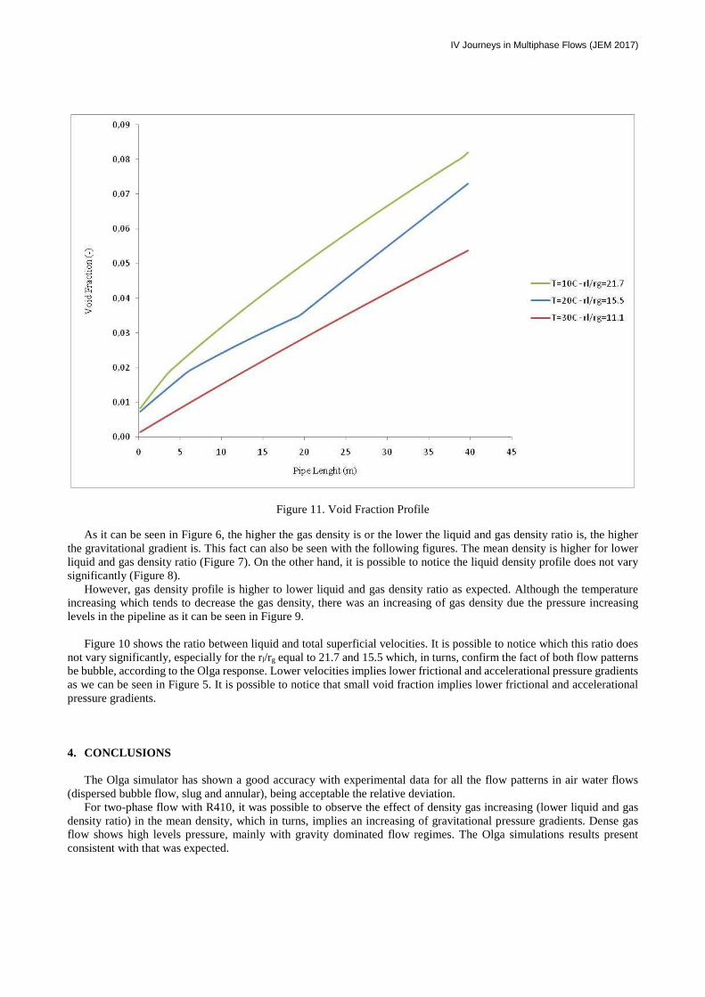
Figure 11. Void Fraction Profile

As it can be seen in Figure 6, the higher the gas density is or the lower the liquid and gas density ratio is, the higher the gravitational gradient is. This fact can also be seen with the following figures. The mean density is higher for lower liquid and gas density ratio (Figure 7). On the other hand, it is possible to notice the liquid density profile does not vary significantly (Figure 8).

However, gas density profile is higher to lower liquid and gas density ratio as expected. Although the temperature increasing which tends to decrease the gas density, there was an increasing of gas density due the pressure increasing levels in the pipeline as it can be seen in Figure 9.

Figure 10 shows the ratio between liquid and total superficial velocities. It is possible to notice which this ratio does

not vary significantly, especially for the rl/rg equal to 21.7 and 15.5 which, in turns, confirm the fact of both flow patterns be bubble, according to the Olga response. Lower velocities implies lower frictional and accelerational pressure gradients as we can be seen in Figure 5. It is possible to notice that small void fraction implies lower frictional and accelerational pressure gradients.

4. CONCLUSIONS

The Olga simulator has shown a good accuracy with experimental data for all the flow patterns in air water flows (dispersed bubble flow, slug and annular), being acceptable the relative deviation.

For two-phase flow with R410, it was possible to observe the effect of density gas increasing (lower liquid and gas density ratio) in the mean density, which in turns, implies an increasing of gravitational pressure gradients. Dense gas flow shows high levels pressure, mainly with gravity dominated flow regimes. The Olga simulations results present consistent with that was expected.


5. REFERENCES

Bueno, L. G. G. Estudo experimental de escoamentos líquido-gás intermitentes em tubulações inclinadas. 151 f. M. Sc. Thesis – Mechanical Engineering, Campinas State University, Campinas, 2010.

Calsep A/S, 2013. PVT Sim Software, Version 21.2.0-FLEXLm Version, <http://www.calsep.com>. DuPont. Thermodynamic Properties of DuPont Suva R-410a Refrigerant. Technical Information, 20p., 2004. Ishikawa, A.; Imai, R.; Tanaka, T, 2014.. “Experimental Study on Two-Phase Flow in Horizontal Tube Bundle Using

SF6-Water”. IHI Engineering Review, v. 46, n. 2, p. 16–21, 2014. Lima, L. E. M. Análise do Modelo de Mistura Aplicado em Escoamentos Isotérmicos Gás-Líquido. 171 f. PhD. Thesis -

Mechanical Engineering, Campinas State University, Campinas, 2011. Owen, D. G. An experimental and theoretical analysis of equilibrium annular flows. 411 p. PhD Thesis - University of

Birmingham, Birmingham, England, abr. 1986. McCain, W.D., 1999. The Properties of Petroleum Fluids. PennWell Publishing Company, Tulsa, Oklahoma, 2nd edition. Rosa, E. S.; Mastelari, N. Desenvolvimento de Técnicas de Medidas, Instrumentação e Medidas em Escoamentos de

Golfadas de Líquido e Gás em Linhas Vertical e Inclinada. Campinas, 2008. 248 p. III Report. Santos, G.R., Loureiro. P.S., 2012. Determinação da Faixa Operacioal de Produção de Poços da Bacia de Santos com

Alta Razão Gás-Óleo. In Proceedings of Rio Oil & Gas Expo and Conference, Rio De Janeiro – RJ, Brazil, IBP 1652_12 10 pages.

Wallis, G.B., 1969. One Dimensional Two-phase Flow. Mc Graw-Hill Book Company, USA, 1st edition. 6. RESPONSIBILITY NOTICE

The authors are the only responsible for the printed material included in this paper.

pressure drop profiles evaluation with dense gas in a …

Documents