pressure drop in pipelines due to pump trip event

ANZIAM J. 57 (MISG2015) pp.M163–M204, 2016 M163

Pressure drop in pipelines due to pump tripevent

Y. M. Stokes1 A. Miller2 G. Hocking3

(Received 23 November 2015; revised 14 September 2016)

Abstract

We consider the pressure pulse or surge in a pipeline due to anunplanned sudden shutdown of a pump system in the pipeline network.This is known as water hammer. Our primary focus is the negativepressure pulse that travels downstream from the pump(s), is reflectedwith a sign reversal from the end, and travels back to the pump(s). Aspart of the preliminary design of a pipeline it is necessary to determinethe minimum head envelope associated with such an event, which isused to determine where surge protection will be needed in the pipeline.Of particular interest is whether the initial head drop at the pump(s)due to a sudden drop of the flow speed to zero, as given by the Joukowskiformula, gives a sufficiently accurate prediction of the minimum headat the pump(s). This minimum head is used to construct the minimum

doi:10.21914/anziamj.v57i0.10277, c© Austral. Mathematical Soc. 2016. PublishedOctober 6, 2016, as part of the Proceedings of the 2015 Mathematics and Statistics inIndustry Study Group. issn 1445-8810. (Print two pages per sheet of paper.) Copies ofthis article must not be made otherwise available on the internet; instead link directly tothe doi for this article. Record comments on this article viahttp://journal.austms.org.au/ojs/index.php/ANZIAMJ/comment/add/10277/0

https://doi.org/10.21914/anziamj.v57i0.10277

http://journal.austms.org.au/ojs/index.php/ANZIAMJ/comment/add/10277/0

Contents M164

head envelope for the downstream pipeline. An examination of therelevant literature along with solution of the water hammer equationsshows that, assuming the flow speed falls instantaneously to zero at thepump(s), the total drop in head at the pump(s) is given by the sum ofthe initial Joukowski head change and the friction loss under normaloperating conditions. While the friction loss may not be significant inshort pipelines, in long pipelines it cannot be neglected.

Contents1 Introduction M165

2 Preliminary pipeline design M166

3 Head loss at the pump: the Joukowski formula M171

4 The water hammer equations M175

5 Solution of the simplified water hammer equations M1775.1 The method of characteristics . . . . . . . . . . . . . . . . M1775.2 An alternative derivation of Joukowski’s formula . . . . . . M1785.3 Numerical solution . . . . . . . . . . . . . . . . . . . . . . M180

6 Simple examples of pump trip events M1836.1 A long pipeline example . . . . . . . . . . . . . . . . . . . M1836.2 A short pipeline example . . . . . . . . . . . . . . . . . . M1956.3 An approximation to the additional fall in head at the pump M197

7 Conclusions M201

1 Introduction M165

1 Introduction

SunWater presented to misg the problem of surge in a long pipeline whenthere is an unplanned sudden shutdown of the pump system, due to a powerfailure, for example. This is known as a “pump-trip event”. When such anevent occurs a positive/negative pressure pulse (or surge) travels along thefull pipeline network upstream/downstream from the location of the tripevent—a phenomenon known as water hammer. The propagation of theinitial pressure pulse/surge transmits the signal along the pipe to bring thewater to a partial stop. This pulse travels at close to the speed of sound,which is typically around 1000m/s in a water-filled steel pipe. It is oftenreflected back at various points along its travel path, for example, due to achange in the pipe diameter, and it is reflected back from the pipe outlet.

The phenomenon of water hammer is commonly associated with the rapidclosure of a valve or tap. In a household system this may cause some violentshuddering. A description of wave propagation upstream due to closure of avalve downstream of a reservoir is given by Chaudhry [1, §1-5] which, while adifferent situation to that considered here, is enlightening. A demonstrationexample of surge due to pump failure in a pumped rising main is given byThorley [8, §2.2]. As a pressure pulse travels over the varying topography,the pressure variations can lead to potentially catastrophic damage to thepipeline system [e.g. 1, §1-10]. SunWater advised the group that a check valveis always included just upstream/downstream of a pump, which closes onpump failure to prevent back flow through the pump and any damage to it.

Sunwater was interested in estimating the magnitude of the pressure surgesdue to a pump-trip event. They were particularly interested in predictingthe downstream surge along the pipe and the need for surge protection thatthis implies, in order to better estimate the cost of the pipeline prior to a fulldetailed design. In particular, they wished to determine the accuracy of theJoukowski formula for prediction of the magnitude of the pressure drop atthe pump(s).


The group broke the study into several problems for investigation:

• the principal features of the preliminary pipeline design process;

• the early stages of a pump-trip event, including the derivation ofJoukowski’s formula which is used to estimate the initial hydraulichead loss; and

• solution of coupled pdes (the water hammer equations) in time andspace for pressure and velocity.

The basic mathematical description of water hammer is traceable back tothe late 1800s through the work of Korteweg [2], Lamb [3] and Skalak [5]. Abrief history on the study of water hammer is given by Chaudhry [1]. Twoimportant names in the field, after whom equations have been named, areJoukowski, whose classic report was first published (in Russian) in 1898, andAllievi who published the general theory of water hammer in 1903 and whois considered to be the originator of the basic water hammer theory with adynamic equation more accurate than that of Korteweg.

2 Preliminary pipeline design

Consider a pipeline extending from a water source at x = 0, where one ormore pumps are located, to a reservoir or outlet at x = L; then x is thehorizontal distance along the pipe, downstream from the pump(s) (Figure 1).The pump(s) provide the necessary energy to transport water along the pipe.This energy must be sufficient to overcome pipe friction and raise the waterfrom the source elevation to the final elevation (which may be more than ahundred kilometres away and hundreds of meters higher) at a satisfactory flowspeed. Neglecting friction losses and assuming a steady flow, the pressure p(x),pipe and ground elevation z(x), and flow speed V(x) at position x along the


pipeline are related by the Bernoulli equation [6]

p

ρg+V2

2g+ z = C, (1)

where ρ is the water density, g is gravitational acceleration and C is a constant.For a pipe of constant diameter, the flow speed V is constant, otherwise,it is V(x) = Q/A(x) where Q is the (constant) volume flux along the pipeand A(x) is the cross-sectional area at position x. Henceforth we assumethat A and the steady flow V are constant along the length of the pipeline.Equation (1) must be modified in the presence of other factors, such asturbulent friction (fx/(2gD))V2, and other head losses β(x)V2/(2g) due tojoins, bends, valves and other pipeline fittings along the pipeline to point xthat disturb the flow, so that

C =p(x)

ρg+

[1+ β(x) +

fx

D

]V2

2g+ z(x), (2)

where D is the internal pipe diameter and f is the friction coefficient. At theend of the pipeline the pressure as the water exits the pipe is assumed to beatmospheric, pA, which gives the value of the constant

C =pA

ρg+

[1+ βL +

fL

D

]V2

2g+ zL, (3)

where zL = z(L) and βL = β(L). Subtracting (3) from (2) and rearranginggives

H(x) = zL +fV2

2Dg(L− x) +

V2

2g(βL − β(x)), (4)

where the hydraulic head

H(x) =p(x) − pA

ρg+ z(x). (5)

Without loss of generality, we take pA = 0 and p(x) to be the pressure inexcess of pA. Plotting H(x) against x, as given by (4), yields the hydraulicgrade line (hgl) for the pipeline under normal operating conditions.


x

z

Pump

Pipeline

Reservoir

Figure 1: Schematic diagram of a pipeline from pump to reservoir, showingthe coordinate system.

In the pipeline design process, the hydraulic head is of major importance.From (5) we see that if H(x) < z(x), that is, the hydraulic head drops belowthe value of the ground elevation at a position x along the pipe, for exampledue to a pressure surge caused by a trip event, then the pressure in thepipe at that position becomes sub-atmospheric (p(x) < pA), or “negative”(taking pA = 0), with negative consequences for the smooth operation ofthe pipeline, including the possibility in extreme cases of catastrophic pipecollapse. Pipeline design involves prediction of the minimum hydraulic headenvelope along the length of the pipeline under the most extreme anticipatedoperating conditions, and prevention of sub-atmospheric pipe pressure bychoice of suitably sized pumps and pipes, and inclusion of surge protectiondevices (surge tanks, air cushion standpipes, etc.) at appropriate locationswhile, at the same time, minimising the cost of the system. Here we focus onthe preliminary design done by SunWater for quotation purposes; the designmust be sufficiently good that SunWater do not under-quote the pipeline orprice themselves out of the market. Subsequently, if the quotation is accepted,then the package watham is used by SunWater for a detailed analysis of


pumps, pipes and surge mitigation devices for a given topography. Thiscomputer package is not used at the initial design phase because of the timetaken both to set up the model and for each simulation.

The cost of pumping is mitigated by reducing the pump size and, therefore,the head at the source, H(0), but this will incur greater costs due to theneed for such things as a significantly larger pipe for a given volume flux, areduction in the volume flux and longer pumping times, additional pumpingstations, and more downstream surge protection.

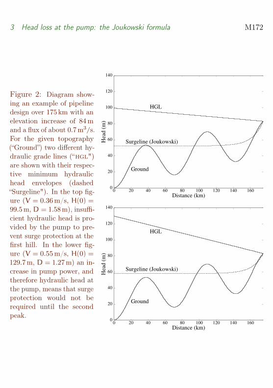
Figure 2 shows an example of the kind of information that is used at theinitial design phase for sizing of pumps and pipes and to place appropriatesurge protection. In constructing this figure we assume that β(x) = 0 (nobends, joins, etc.). The hgl is shown under normal operating conditions;intersection of the hgl with the ground elevation indicates the need fora significant modification of the pipeline design, such as another pumpingstation or a bigger source pump to preclude subatmospheric pressure inthe pipe under normal operating conditions. The curve labelled “Surgeline”is an estimate of the minimum hydraulic head due to the pressure surgefollowing the worst-case scenario of the sudden loss of all pumps, that is, acomplete pump-trip event, with associated check-valve closure. Intersectionof this curve with the ground signals possible catastrophic pipe failure dueto subatmospheric pressure and, therefore, the need for some kind of surgeprotection. Although a pipe in practice withstands some negative pressure,at the preliminary design phase any negative pressure is taken as an indicatorof the need for surge protection.

A good estimate of the surgeline is critical to obtaining a good preliminarypipeline design with necessary, but not overly excessive, surge protection. Acritical aspect of obtaining the surgeline is determining the initial change inhead, ∆HJ< 0, at the pump(s) when they fail suddenly. This was the keyquantity that the study group was asked to consider. It is normally calculatedusing the Joukowski formula, which relates a velocity change to a pressurechange as discussed in Section 3, and assuming that the flow speed at the


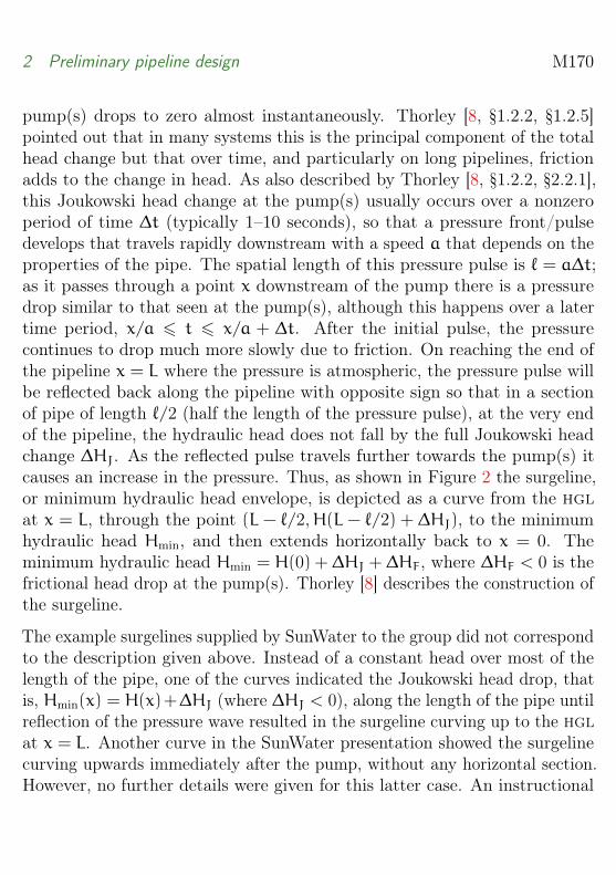
pump(s) drops to zero almost instantaneously. Thorley [8, §1.2.2, §1.2.5]pointed out that in many systems this is the principal component of the totalhead change but that over time, and particularly on long pipelines, frictionadds to the change in head. As also described by Thorley [8, §1.2.2, §2.2.1],this Joukowski head change at the pump(s) usually occurs over a nonzeroperiod of time ∆t (typically 1–10 seconds), so that a pressure front/pulsedevelops that travels rapidly downstream with a speed a that depends on theproperties of the pipe. The spatial length of this pressure pulse is ` = a∆t;as it passes through a point x downstream of the pump there is a pressuredrop similar to that seen at the pump(s), although this happens over a latertime period, x/a 6 t 6 x/a + ∆t. After the initial pulse, the pressurecontinues to drop much more slowly due to friction. On reaching the end ofthe pipeline x = L where the pressure is atmospheric, the pressure pulse willbe reflected back along the pipeline with opposite sign so that in a sectionof pipe of length `/2 (half the length of the pressure pulse), at the very endof the pipeline, the hydraulic head does not fall by the full Joukowski headchange ∆HJ. As the reflected pulse travels further towards the pump(s) itcauses an increase in the pressure. Thus, as shown in Figure 2 the surgeline,or minimum hydraulic head envelope, is depicted as a curve from the hglat x = L, through the point (L − `/2,H(L − `/2) + ∆HJ), to the minimumhydraulic head Hmin, and then extends horizontally back to x = 0. Theminimum hydraulic head Hmin = H(0) + ∆HJ + ∆HF, where ∆HF < 0 is thefrictional head drop at the pump(s). Thorley [8] describes the construction ofthe surgeline.

The example surgelines supplied by SunWater to the group did not correspondto the description given above. Instead of a constant head over most of thelength of the pipe, one of the curves indicated the Joukowski head drop, thatis, Hmin(x) = H(x)+∆HJ (where ∆HJ < 0), along the length of the pipe untilreflection of the pressure wave resulted in the surgeline curving up to the hglat x = L. Another curve in the SunWater presentation showed the surgelinecurving upwards immediately after the pump, without any horizontal section.However, no further details were given for this latter case. An instructional


document prepared by the large German water industry company ksb [4],also shows the surgeline as sloping upwards towards the hgl immediatelyafter the pump. This surgeline was based on measured data from a pipelineinstallation following a pump trip, although again few details are given [4,Figure 2.1-b]. There would, therefore, seem to be no universal consensus onthe form that the surgeline takes, or its dependence on specific pipeline andoperational parameters. Thorley [8, §1.2.4] describes a ‘rapid’ event wherethe pipeline is sufficiently short that the pressure pulse travels to the reservoirand back to the pump in a time less than the time ∆t over which the pressureat the pump(s) falls by the Joukowski head change. In this situation thesurgeline would be a monotonic increasing curve from x = 0 to x = L as inthe last two examples.

The two simple cases in Figure 2 show one in which the pump head is notsufficient to prevent the need for surge protection on the first hill. Theassociated surgeline shows that some form of surge protection would berequired on both high points. The second case (right-hand panel) has a largerinitial hydraulic head and a surgeline that indicates that surge protectionis not needed until the second peak. Using such a simple tool, a pipeline,including pipe sizes, pump sizes and locations and size and position of surgeprotection, can be designed and optimised to minimize cost. However, becauseof the interdependence of the pipe diameter and material, flow speed, frictionfactor, required head and hence pump size, it is not a simple task to obtain asuitable design.

3 Head loss at the pump: the Joukowskiformula

The first step in predicting a surgeline is to determine the change in thehydraulic head at the pump immediately after a trip event. This is foundby Newton’s 2nd law to depend on the change in the velocity ∆V, and the


Figure 2: Diagram show-ing an example of pipelinedesign over 175 km with anelevation increase of 84mand a flux of about 0.7m3/s.For the given topography(“Ground”) two different hy-draulic grade lines (“hgl")are shown with their respec-tive minimum hydraulichead envelopes (dashed“Surgeline"). In the top fig-ure (V = 0.36m/s, H(0) =99.5m, D = 1.58m), insuffi-cient hydraulic head is pro-vided by the pump to pre-vent surge protection at thefirst hill. In the lower fig-ure (V = 0.55m/s, H(0) =129.7m, D = 1.27m) an in-crease in pump power, andtherefore hydraulic head atthe pump, means that surgeprotection would not berequired until the secondpeak.

0

20

40

60

80

100

120

140

0 20 40 60 80 100 120 140 160

Hea

d (

m)

Distance (km)

HGL

Ground

Surgeline (Joukowski)

0

20

40

60

80

100

120

140

0 20 40 60 80 100 120 140 160

Hea

d (

m)

Distance (km)

HGL

Ground

Surgeline (Joukowski)


propagation speed of the pulse a, also called the celerity, as encapsulated inthe Joukowski formula,

∆H =a

g∆V . (6)

A straightforward derivation of this formula is given by Chaudhry [1, §1.4],which is not repeated here. The misg group checked this derivation andfound it to be correct. Note that ∆V < 0 is a drop in the flow speed whichwill result in a drop in the hydraulic head, ∆H < 0.

Chaudhry [1] also shows that, for a slightly compressible fluid in a rigid pipe,the propagation speed a =

√K/ρ where ρ is the (initial) fluid density and

K = ρdp/dρ is the bulk modulus of elasticity of the fluid. The large valueof K for water (around 2.2GPa) justifies the incompressible approximationin most flow situations. However, in some transient flow situations such asin long pipelines, compressibility has a significant effect, since a pressuredisturbance may take appreciable time to transit the length of the pipe. The“effective compressibility” of the pipe-fluid system has contributions not onlyfrom the actual compressibility of the water, but also from the elastic responseof the pipe itself, which will expand or contract radially in response to pressuredisturbances. The pipe elasticity will increase the effective compressibilityover that of the fluid alone, that is, decrease the effective bulk modulus ofelasticity compared to that of the fluid. A modified formula for the wavespeed a for thin-walled elastic conduits is [1]

a =

√K

ρ

(1

1+ (K/E)(D/s)c

), (7)

where E is the Young’s modulus of the pipe material, D is the internal pipediameter, s is the thickness of the pipe wall, and c is a dimensionless quantitythat takes different values depending on the extent to which the pipe isable to expand axially. If there is no constraint on local axial expansion ofthe pipe, such as would be the case if there are frequent axial expansionjoints, then c = 1. If the pipe is rigidly restrained in the axial direction,then c = 1 − ν2 where ν is Poisson’s ratio. Intermediate degrees of axial


constraint correspond to values of c between these limits. This formula for ais simply the propagation speed in a rigid pipe multiplied by a correctionfactor for pipe elasticity. Since the correction factor will always be less thanone, the wave propagation speed is reduced compared to that in a rigid pipe.There can be considerable variation in this correction factor between differentpipe materials whose Young’s moduli may vary between 200GPa for cementlined steel pipes and 1GPa for plastic hdpe pipes. The bulk modulus ofelasticity of water, K, is significantly reduced by the presence of small bubblesand dissolved air. Typically for steel pipes, a is of the order of 1000m/s,which is to be compared to the speed of sound in water in a rigid pipe ofaround 1500m/s.

The initial drop in flow speed at the pump, which gives the change in hydraulichead via (6), depends on whether a check valve is used to prevent back flow.Since SunWater advised that a check valve is always used for protection of thepump(s), it was assumed that, to a good approximation, the water is broughtto an instantaneous stop by the valve, which is also the worst case scenario.

As an example, consider a steady state flow with speed V0 in the direction ofincreasing x, and let the head at some point P in the pipe be HP. If the flowat P is suddenly stopped, then there will be an instantaneous jump in headat P of

∆H =a

g∆V =

a

g(0− V0) = −

a

gV0;

that is, there is a decrease in the hydraulic head of magnitude aV0/g. Con-versely, there will be a rise in head of the same magnitude at P if the initialsteady-state flow velocity is V0 < 0, that is in the direction of decreasing x.

With the wave speed computed from (7) and the change in hydraulic headat the pump due to a trip event computed by the Joukowski formula, it is asimple exercise to draw the surgeline neglecting any frictional component.


4 The water hammer equations

The propagation of the pulse along the pipeline following a trip event, ismore accurately described by a set of partial differential equations, known asthe water hammer equations, much like those for sound propagation. Thesewere solved to obtain the surgeline more accurately for comparison with thatdetermined by a preliminary pipeline design as described in Section 2. Theseequations are nonlinear, which means that they cannot be solved exactly.However, they can be solved quite accurately on a computer. The componentof watham that resolves the pressures in the pipe solves these equations.

The equations describing transient flow in the pipe are

g∂H

∂x+

f

2DV |V |+ V

∂V

∂x+∂V

∂t= 0, (8)

a2

g

∂V

∂x+ V

∂H

∂x+∂H

∂t= 0, (9)

where H(x, t) and V(x, t) are the hydraulic head and flow speed averagedover the cross section of the pipe at position x along the pipe at time t;writing V |V | instead of V2 in (8) allows for reverse flow. As before, D is thediameter of the pipe, assumed to be constant, a is the celerity or speed ofpropagation of a pressure disturbance in the pipe-fluid system (Section 3),and f is the friction factor which will be discussed next. Equations (8) and (9)represent the conservation of momentum in the axial direction and of fluidmass, respectively. Two key assumptions implicit in these one-dimensionalequations are:

• any curvature in the pipeline, in either the horizontal or vertical planes,is small relative to the inverse diameter of the pipe, which justifiesusing the distance x as a valid one-dimensional axial coordinate in theequations; and

• the flow in the pipe is turbulent and reasonably approximates “plugflow” with near uniform velocity, density and pressure profiles across


each cross section, so that use of cross-section-averaged quantities inthe equations is justified.

Equations (8) and (9) may be further simplified because the flow speed Vis much less than the wave propagation speed a; that is, V/a � 1. Anondimensionalisation, using length scale L, fluid velocity scale V � a

and time scale L/a, shows that the nonlinear convective terms V∂V/∂xand V∂H/∂x are small relative to the other terms, justifying their neglect.This is a very typical simplification of the water hammer equations [e.g. 1].

We come now to a discussion of the friction factor f appearing in (8). Thisarises from the Darcy–Weisbach expression for the head loss in a pipe understeady state conditions,

∆H

∆x= −f

V2

2gD, (10)

which, incidentally, may be determined from (8) if we set ∂V/∂t = 0 (steadyflow) and ∂V/∂x = 0 (incompressible flow), or by taking the x-derivativeof the Bernoulli equation (4). The value of the friction factor f is obtainedby semi-empirical means, usually by reference to the Moody diagram [6], orother related analytical expressions such as the implicit Colebrook equationor the explicit formula of Swamee & Jain [7]. Although the friction factoris non-dimensional, it is not necessarily constant for any given pipe. Fromdimensional considerations, we expect that

f = f(Re, ε/D),

where Re = VDρ/µ is the Reynolds number of the flow for a fluid withviscosity µ, and ε is a roughness parameter characterising the size of theroughness protrusions on the wall of the pipe. A feature of the Moody diagramis that for a pipe of roughness ε/D there is a value of Re above which the flowis “completely turbulent” and f is, essentially, independent of Re. Howeverbelow this Reynolds number f depends on both Re and ε/D, so that thehead loss in (10) will not be quadratic in V . Typically, the head loss behaveswith a lower exponent of V than two, and for laminar flow, is linear in V.

5 Solution of the simplified water hammer equations M177

Strictly speaking, the friction factor is defined and determined under steadyflow conditions, so its use in (8) assumes that this steady state value is alsoreasonable under transient flow conditions. In reality, it takes a finite timefor steady state conditions to be established, so the use of steady state valuesin unsteady flows does not strictly follow, although invariably in practicalcalculations, the steady state value is used.

5 Solution of the simplified water hammerequations

5.1 The method of characteristics

Our task is now to solve the simplified water hammer equations

g∂H

∂x+

f

2DV |V |+

∂V

∂t= 0, (11)

a2

g

∂V

∂x+∂H

∂t= 0, (12)

subject to initial conditions H(x, 0) given by (4) and V(x, 0) the specifiedconstant steady state velocity, with boundary conditions V(0, t) = 0 andH(L, t) = zL (where we have set pA = 0). For this we use the method ofcharacteristics, and so introduce the new variables

ξ = x− at, η = x+ at.

Transforming the derivatives in (11) and (12) to derivatives with respect to ξand η, we obtain after some manipulation

∂H

∂ξ−a

g

∂V

∂ξ+

f

4gDV |V | = 0, (13)

∂H

∂η+a

g

∂V

∂η+

f

4gDV |V | = 0. (14)


Figure 3 shows the orientation of the lines of constant ξ and constant η inthe x-t plane. Now integrating (13) along a line of constant η and (14) alonga line of constant ξ leads to(

H−a

gV

)∣∣∣∣ξ1ξ0

= −

∫ξ1ξ0

f

4gDV |V |dξ (η = constant), (15)(

H+a

gV

)∣∣∣∣η1η0

= −

∫η1η0

f

4gDV |V |dη (ξ = constant), (16)

and returning to the original variables x and t gives(H−

a

gV

)∣∣∣∣x1x0

= −

∫x1x0

f

2gDV |V |dx (x+ at = constant), (17)(

H+a

gV

)∣∣∣∣x1x0

= −

∫x1x0

f

2gDV |V |dx (x− at = constant). (18)

These equations are the basis of the numerical solution described in Subsec-tion 5.3.

5.2 An alternative derivation of Joukowski’s formula

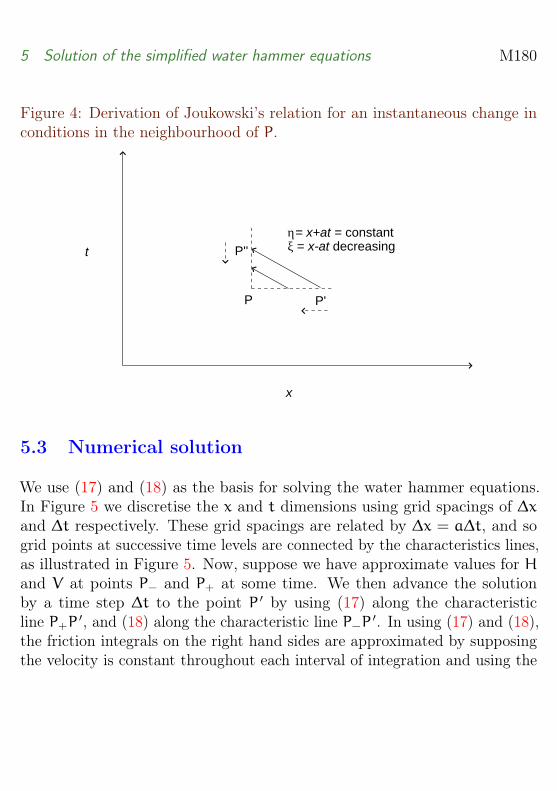
It is of interest to first use (17) and (18) to derive Joukowski’s formula forthe instantaneous response to a change of conditions. With reference toFigure 4, consider the characteristic η = constant joining points P ′ and P ′′ inthe x-t plane. Let P ′ → P, then P ′′ also approaches P, and the distance P ′P ′′

approaches 0. Thus, in the limit, from (17)

limP ′′→P

(H−

a

gV

)= limP ′→P

(H−

a

gV

).

Writing

∆H = limP ′′→P

H− limP ′→P

H and ∆V = limP ′′→P

V − limP ′→P

V ,


Figure 3: The orientation of the characteristics ξ = constant and η = constantin the x-t plane.

t

x

ξ = x-at = constantη = x+at increasing

η= x+at = constantξ = x-at decreasing

we obtain Joukowski’s relation

∆H =a

g∆V . (19)

If H and V are continuous in the neighbourhood of P, then both sides ofthis equation are zero and the relationship is trivial. However, if there arediscontinuous changes in H and V , then (19) shows how these must be related.

Joukowski’s relation is completely general, and applies to any sudden changein the pipeline conditions. However, it only gives the instantaneous localresponse. As discussed in Section 6, the longer term response, and theresponse some distance from the change, are quite different due to frictionaltransmission effects.


Figure 4: Derivation of Joukowski’s relation for an instantaneous change inconditions in the neighbourhood of P.

t

x


P

P''

P'

5.3 Numerical solution

We use (17) and (18) as the basis for solving the water hammer equations.In Figure 5 we discretise the x and t dimensions using grid spacings of ∆xand ∆t respectively. These grid spacings are related by ∆x = a∆t, and sogrid points at successive time levels are connected by the characteristics lines,as illustrated in Figure 5. Now, suppose we have approximate values for Hand V at points P− and P+ at some time. We then advance the solutionby a time step ∆t to the point P ′ by using (17) along the characteristicline P+P ′, and (18) along the characteristic line P−P ′. In using (17) and (18),the friction integrals on the right hand sides are approximated by supposingthe velocity is constant throughout each interval of integration and using the


Figure 5: The basis of the explicit time stepping scheme for numericallysolving (17) and (18). The spatial discretisation parameter ∆x and the timestep ∆t are related by ∆x = a∆t .

t

x

ξ = x-at = constantη = x+at increasing


∆x

∆tP- P

P'

P+

P'

P-

P'

P+

right handboundary

left handboundary

interior point

P P

known velocities at the points P+ and P−, respectively:(H−

a

gV

)∣∣∣∣P ′

P+

≈ f∆x

2gDV(P+)|V(P+)|; (20)(

H+a

gV

)∣∣∣∣P ′

P−

≈ −f∆x

2gDV(P−)|V(P−)|. (21)

In (17), x is decreasing along the characteristic line P+P ′, and so there isan implied negative sign in the evaluation of the integral on the right handside, which leads to a positive sign in the right hand side of the first equationabove. In this way, we obtain values for

H−a

gV and H+

a

gV

at the new point P ′. Solving this non-singular 2× 2 linear system, gives usvalues for H and V at P ′.


The above description relates to interior points along the pipeline. Thesituation is usually slightly simpler at the endpoints of the pipeline, as thereare specified boundary conditions at these points. These boundary conditionsprovide a relationship involving H and V at each of the boundary points. Asan example, suppose there is a specified head boundary condition H = HL atthe right hand boundary in Figure 5. We use (18) to advance the solutionfrom P− to P ′ along the characteristic which gives us the value of H+(a/g)Vat P ′. Since we know H at P ′ from the boundary condition, we are ableto determine V. In the same way, if the boundary condition is a specifiedvelocity, V = VL, then H is determined. More generally, a boundary conditioninvolving some relationship between H and V , such as might arise from theoperating curves of a valve, pump or other fitting, is solved simultaneouslywith this advanced value of H+(a/g)V at P ′, to again obtain values for both Hand V at P ′. An analogous situation applies at a left hand boundary point,except that (17) is used to advance the solution for H− (a/g)V along P+P ′,as depicted in Figure 5.

Returning to the approximation used in the evaluation of the friction integrals,an alternative, and presumably more accurate approach would be to use atrapezoidal rule approximation. In the notation of Figure 5, this wouldbecome for an interior point P ′

(H−

a

gV

)∣∣∣∣P ′

P+

≈ f∆x

4gD[V(P ′)|V(P ′)|+ V(P+)|V(P+)|] ,(

H+a

gV

)∣∣∣∣P ′

P−

≈ −f∆x

4gD[V(P ′)|V(P ′)|+ V(P−)|V(P−)|] .

This is a nonlinear system of equations for the unknowns V(P ′) and H(P ′).(It is quadratic, although we do not make explicit use of this.) As f and V areusually small, the system is readily solved by a simple iteration that uses themost recent iterate for V(P ′) in the trapezoidal rule expression on the righthand side, and then solves the left hand side 2× 2 linear system for updatedvalues of V(P ′) and H(P ′). This process is repeated until sufficient accuracy is

6 Simple examples of pump trip events M183

achieved. The iteration is started by using, as the initial iterate, the solutiondescribed earlier which took the velocity to be constant throughout eachinterval of integration using the known velocities at the points P+ and P−respectively. A similar approach is taken with the friction integrals appearingin the boundary conditions.

Our experience in running a number of examples, such as those describednext in Section 6, is that the use of this trapezoidal rule approximation hasonly a negligible effect on the solution. Therefore, for most practical purposes,the simpler constant-velocity approximation and the resulting equations (20)and (21) should be sufficient.

6 Simple examples of pump trip events

6.1 A long pipeline example

To try to understand the transients associated with a pump trip event, considerthe simple case illustrated in Figure 6. This shows the steady state hydraulicgrade line of a pipeline connecting two reservoirs. Water is transported fromthe higher reservoir to the lower reservoir over a distance of 200 km. Midwaybetween the two reservoirs at x = 0 there is a pump that provides additionalhead to overcome the frictional losses in the pipeline. In reality, there maywell be additional pumping locations and a number of surge protection unitsin the pipeline; however, for the purposes of seeking to intuitively understandthe response to a pump trip event, we restrict ourselves to this simplifiedlayout.

The various hydraulic parameters used are shown in Figure 6. The frictionfactor is based on the Moody diagram for a cast iron pipe with roughnessε = 0.25mm. This places the flow conditions in the transition zone betweenthe smooth pipe limit (where f = f(Re) only) and the rough pipe (completeturbulence) limit (where f = f(ε/D) only). For velocities in the range 0.1–


Figure 6: The hydraulic grade line of a simple pipe system in steady stateconnecting two reservoirs with an intermediate pump. The flow rate is 1ms−1

and the pump boosts the head by ∆H = 200m. The hydraulic parametersused in the model are shown.

H = 100m

H = 300m

Pump ∆H = 200m

H = 233.3mconstant head reservoir

H = 166.6mconstant head reservoir

direction of flowv = 1 ms-1length = 100km

length = 100km

Parameters: f = 0.02 D = 0.75 m a = 1 km s-1

g = 10 ms-2

1.0ms−1, the Moody diagram gives f ≈ 0.022−0.017. We therefore take theconstant value f = 0.02 over this entire velocity range.

Figure 6 notes the values for the steady state solution of this situation. Wenow imagine that at time t = 0 the pump at x = 0 trips (shuts downsuddenly), the check valve (instantaneously) closes, and flow immediatelyceases just upstream and downstream of the pump, that is, at x = 0− andx = 0+. This isolates the upstream and downstream flows, which now evolveindependently. In the transient flows that take place, we assume that V = 0at x = 0, and H remains constant at each of the reservoir ends of the pipeline.The transient behaviour in the pipeline has been simulated for 200 s, whichcorresponds to the time for the pressure pulses to travel the 200 km to thereservoirs and back again to the pump at a speed of 1000m/s.

We first consider the downstream side of the pump. Figure 7 shows the time


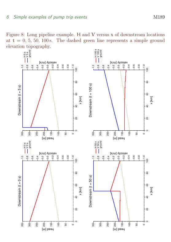
evolution of H and V at the pump and at locations 5 km, 50 km and 100 kmdownstream for times from 0 to 200 s. (Recall that the lower reservoir is 100 kmdownstream.) Figures 8 and 9 show H and V along the entire downstreamportion of the pipeline at the selected times of 0, 5, 50, 100, 105, 150 and 200 safter tripping. Figures 8 and 9 also depict a simple linear ground elevationtopography from z(0) = 100m to z(L) = 166.6m, which is used in ourdiscussion at the end of this subsection.

The x = 0 km plot shows that the head on the downstream side of the pumpsuddenly falls by 100m just after the trip at t = 0. This is consistent with theJoukowski equation, as we would expect, corresponding to a sudden changeof velocity of −1ms−1 as flow at the pump ceases. However, after this initialsharp drop, the head continues to fall in an almost linear fashion with timefor the remainder of the 200 s of the simulation. The reason for this is seenby looking at the other plots in Figure 7. At the 5 km and 50 km locationsthe initial downstream travelling pulse is reduced in magnitude (the headdrop successively reduces) and is insufficient to completely stop the flow. Theoriginal fluid velocity of 1ms−1 is only reduced to about 0.03 and 0.3ms−1

respectively at these locations because frictional effects are damping themagnitude of the pressure pulse. Thus, after this initial pressure pulse haspassed a location, the fluid continues to move downstream with a reducedvelocity, and this reduced velocity is greater the further down the pipe we go.Thus, any element of fluid is gradually drawing away from the fluid behind it,and so we expect some rarefaction or thinning of the fluid to occur, whichresults in a further falling of head behind the pulse as it travels towards thedownstream reservoir.

From the plots in Figure 7, we see that at t = 100 s, which is the time atwhich the initial pressure pulse reaches the downstream reservoir, the headat 0 km, 5 km and 50 km are all approximately equal at 135m. (This is alsoseen from the t = 100 s plot in Figure 8, which shows that the head is almostuniform behind the pulse.) This pressure head represents a further drop inhead of 65m, on top of the initial Joukowski drop of 100m at the pump.At t = 100 s, the pulse reaches the downstream reservoir and there is some


“reflection”, depending upon the mismatch of head at the reservoir between theconstant head terminus condition and the arriving pressure pulse. We look atthis in the next paragraph. However, first note that it takes another 100 sbefore this “reflected” pulse reaches the pump. In the meantime, the headat the pump continues to fall. As shown in Figure 9 at 200 s, just as thereflected pulse reaches the pump, the head at the pump has already fallen toapproximately 80m, which is 120m below the initial Joukowski drop of 100m.We therefore see that, depending on the circumstances, the head drop at thepump can be significantly greater than that predicted by the instantaneousJoukowski result—in this case over double. Should the head fall below groundlevel, this may have potentially grave consequences such as severe mechanicaldamage to the pipe, and even pipe collapse.

The t = 100 s plot in Figure 8 shows the situation as the downstream pulsearrives at the reservoir. The head in the pipe is substantially uniform, butit is below the constant head at the reservoir. This mismatch triggers aninstantaneous change in velocity at the reservoir end of the pipe (again,incidentally, given by the Joukowski formula) and a reflected positive pressurepulse now traves upstream from the reservoir. As this pulse travels backtowards the pump a reverse flow develops in the pipe. As the t = 200 s plot inFigure 9 shows, when this pulse reaches the pump, the flow conditions alongthe pipe approximate a uniform reverse hydraulic grade line with a uniformreverse flow. This reverse flow velocity is approximately 30% of the originalflow velocity and the reverse hydraulic gradient is about 40% of its originalvalue.

That the head in the pipe is below the head at the reservoir at t = 100 scan also have serious consequences upstream from the reservoir. Dependingon the local topography, the water pressure in the pipe may well fall belowatmospheric, or even approach a vacuum. Again, this is undesirable and maylead to serious pipe damage or collapse.

To make the discussion more concrete, consider the case of the simple groundelevation topography shown by the dashed lines in Figures 8 and 9, namely


a constant upward sloping topography from the pump to the downstreamreservoir. Here the pump is taken to be at an elevation of 100m. Figure 8shows that at some time between 50 s and 100 s after the trip, the head curvefalls beneath the elevation line. This first occurs somewhere near x = 75 kmdownstream from the pump. Once this happens, the pressure in the pipelinebecomes negative. Recall that we are using gauge pressure, with atmosphericpressure being the reference pressure. Thus, the pressure at that point fallsbelow atmospheric, which, as just mentioned, can have serious undesirableconsequences. So for this simple example, the above analysis would suggestthe need to introduce some surge protection near this point.

The actual numerical values presented here are obviously configuration specific;however, the overall principle is clear, namely that, due to frictional effects,there is a continuing head drop on the downstream side of the pump after theinitial step change. This can be substantially greater than the instantaneousdrop predicted by Joukowski, and this drop continues until the reflected pulsereaches the pump from the reservoir. The reflected pulse brings with it areverse flow that tends to increase the head at the pump.

Now consider the upstream side of the pump. Figure 10 shows the timeevolution of H and V at the pump and at locations 5 km, 50 km and 100 kmupstream for times from 0 to 200 s. (Recall that the higher reservoir is located100 km upstream.) Figures 11 and 12 show H and V along the entire upstreamportion of the pipeline at the selected times of 0, 5, 50, 100, 105, 150 and 200 safter the trip.

The x = 0 km plot shows that now there is an initial jump in head of 100mon the upstream side of the pump—from 100m to 200m. (Again, this iswhat the Joukowski formula predicts from the assumed instantaneous changein fluid velocity at the pump.) The head, and therefore also the pressure,then continues to rise at the pump in an almost linear fashion with timeuntil t = 200 s, when the reflected pressure pulse from the upstream reservoirreaches the pump. The total increase in head by 200 s is a little over 200m,corresponding to a pressure increase of some 2MPa. The reason for this


Figure 7: Long pipeline example. H and V versus t for downstream locationsx = 0, 5, 50, 100 km.

Do

wn

str

ea

m (

x =

0 k

m)

tim

e [

s]

05

01

00

15

02

00

head [m]

050

10

0

15

0

20

0

25

0

30

0

35

0

velocity [m/s]

-1.0

-0.8

-0.6

-0.4

-0.2

0.0

0.2

0.4

0.6

0.8

1.0

H 0

km

V 0

km

Do

wn

str

ea

m (

x =

5 k

m)

tim

e [

s]

05

01

00

15

02

00

head [m]

050

10

0

15

0

20

0

25

0

30

0

35

0

velocity [m/s]

-1.0

-0.8

-0.6

-0.4

-0.2

0.0

0.2

0.4

0.6

0.8

1.0

H 5

km

V 5

km

Do

wn

str

ea

m (

x =

10

0 k

m)

tim

e [

s]

05

01

00

15

02

00

head [m]

050

10

0

15

0

20

0

25

0

30

0

35

0

velocity [m/s]

-1.0

-0.8

-0.6

-0.4

-0.2

0.0

0.2

0.4

0.6

0.8

1.0

H 1

00

km

V 1

00

km

Do

wn

str

ea

m (

x =

50

km

)

tim

e [

s]

05

01

00

15

02

00

head [m]

050

10

0

15

0

20

0

25

0

30

0

35

0

velocity [m/s]

-1.0

-0.8

-0.6

-0.4

-0.2

0.0

0.2

0.4

0.6

0.8

1.0

H 5

0 k

m V

50

km


Figure 8: Long pipeline example. H and V versus x of downstream locationsat t = 0, 5, 50, 100 s. The dashed green line represents a simple groundelevation topography.

Do

wn

str

ea

m (

t =

0 s

)

x [

km

]

02

04

06

08

01

00

head [m]

050

10

0

15

0

20

0

25

0

30

0

35

0

velocity [m/s]

-1.0

-0.8

-0.6

-0.4

-0.2

0.0

0.2

0.4

0.6

0.8

1.0

H 0

s V

0 s

gro

un

d

Do

wn

str

ea

m (

t =

5 s

)

x [

km

]

02

04

06

08

01

00

head [m]

050

10

0

15

0

20

0

25

0

30

0

35

0

velocity [m/s]

-1.0

-0.8

-0.6

-0.4

-0.2

0.0

0.2

0.4

0.6

0.8

1.0

H 5

s V

5 s

gro

un

d

Do

wn

str

ea

m (

t =

10

0 s

)

x [

km

]

02

04

06

08

01

00

head [m]

050

10

0

15

0

20

0

25

0

30

0

35

0

velocity [m/s]

-1.0

-0.8

-0.6

-0.4

-0.2

0.0

0.2

0.4

0.6

0.8

1.0

H 1

00

s V

10

0 s

gro

un

d

Do

wn

str

ea

m (

t =

50

s)

x [

km

]

02

04

06

08

01

00

head [m]

050

10

0

15

0

20

0

25

0

30

0

35

0

velocity [m/s]

-1.0

-0.8

-0.6

-0.4

-0.2

0.0

0.2

0.4

0.6

0.8

1.0

H 5

0 s

V 5

0 s

gro

un

d


Figure 9: Long pipeline example. H and V versus x of downstream locationsat t = 105, 150, 200 s. The dashed green line represents a simple groundelevation topography.

Do

wn

str

ea

m (

t =

10

5 s

)

x [

km

]

02

04

06

08

01

00

head [m]

050

10

0

15

0

20

0

25

0

30

0

35

0

velocity [m/s]

-1.0

-0.8

-0.6

-0.4

-0.2

0.0

0.2

0.4

0.6

0.8

1.0

H 1

05

s V

10

5 s

gro

un

d

Do

wn

str

ea

m (

t =

15

0 s

)

x [

km

]

02

04

06

08

01

00

head [m]

050

10

0

15

0

20

0

25

0

30

0

35

0

velocity [m/s]

-1.0

-0.8

-0.6

-0.4

-0.2

0.0

0.2

0.4

0.6

0.8

1.0

H 1

50

s V

15

0 s

gro

un

d

Do

wn

str

ea

m (

t =

20

0 s

)

x [

km

]

02

04

06

08

01

00

head [m]

050

10

0

15

0

20

0

25

0

30

0

35

0

velocity [m/s]

-1.0

-0.8

-0.6

-0.4

-0.2

0.0

0.2

0.4

0.6

0.8

1.0

H 2

00

s V

20

0 s

gro

un

d


Figure 10: Long pipeline example. H and V versus t for upstream locationsx = 0, 5, 50, 100 km.

Up

str

ea

m (

x =

0 k

m)

tim

e [

s]

05

01

00

15

02

00

head [m]

050

10

0

15

0

20

0

25

0

30

0

35

0

velocity [m/s]

-1.0

-0.8

-0.6

-0.4

-0.2

0.0

0.2

0.4

0.6

0.8

1.0

H 0

km

V 0

km

Up

str

ea

m (

x =

-5

km

)

tim

e [

s]

05

01

00

15

02

00

head [m]

050

10

0

15

0

20

0

25

0

30

0

35

0

velocity [m/s]

-1.0

-0.8

-0.6

-0.4

-0.2

0.0

0.2

0.4

0.6

0.8

1.0

H 5

km

V 5

km

Up

str

ea

m (

x =

-1

00

km

)

tim

e [

s]

05

01

00

15

02

00

head [m]

050

10

0

15

0

20

0

25

0

30

0

35

0

velocity [m/s]

-1.0

-0.8

-0.6

-0.4

-0.2

0.0

0.2

0.4

0.6

0.8

1.0

H 1

00

km

V 1

00

km

Up

str

ea

m (

x =

-5

0 k

m)

tim

e [

s]

05

01

00

15

02

00

head [m]

050

10

0

15

0

20

0

25

0

30

0

35

0

velocity [m/s]

-1.0

-0.8

-0.6

-0.4

-0.2

0.0

0.2

0.4

0.6

0.8

1.0

H 5

0 k

m V

50

km


Figure 11: Long pipeline example. H and V versus x of upstream locationsat t = 0, 5, 50, 100 s.

Upstr

eam

(t =

0 s

)

x [km

]

-10

0-8

0-6

0-4

0-2

00

head [m]

050

10

0

15

0

20

0

25

0

30

0

35

0

velocity [m/s]

-1.0

-0.8

-0.6

-0.4

-0.2

0.0

0.2

0.4

0.6

0.8

1.0

H 0

s V

0 s

Upstr

eam

(t =

5 s

)

x [km

]

-10

0-8

0-6

0-4

0-2

00

head [m]

050

10

0

15

0

20

0

25

0

30

0

35

0

velocity [m/s]

-1.0

-0.8

-0.6

-0.4

-0.2

0.0

0.2

0.4

0.6

0.8

1.0

H 5

s V

5 s

Upstr

eam

(t =

100 s

)

x [km

]

-10

0-8

0-6

0-4

0-2

00

head [m]

050

10

0

15

0

20

0

25

0

30

0

35

0

velocity [m/s]

-1.0

-0.8

-0.6

-0.4

-0.2

0.0

0.2

0.4

0.6

0.8

1.0

H 1

00

s V

10

0 s

Upstr

eam

(t =

50 s

)

x [km

]

-10

0-8

0-6

0-4

0-2

00

head [m]

050

10

0

15

0

20

0

25

0

30

0

35

0

velocity [m/s]

-1.0

-0.8

-0.6

-0.4

-0.2

0.0

0.2

0.4

0.6

0.8

1.0

H 5

0 s

V 5

0 s


Figure 12: Long pipeline example. H and V versus x of upstream locationsat t = 105, 150, 200 s.

Up

str

ea

m (

t =

10

5 s

)

x [

km

]

-10

0-8

0-6

0-4

0-2

00

head [m]

050

10

0

15

0

20

0

25

0

30

0

35

0

velocity [m/s]

-1.0

-0.8

-0.6

-0.4

-0.2

0.0

0.2

0.4

0.6

0.8

1.0

H 1

05

s V

10

5 s

Up

str

ea

m (

t =

15

0 s

)

x [

km

]

-10

0-8

0-6

0-4

0-2

00

head [m]

050

10

0

15

0

20

0

25

0

30

0

35

0

velocity [m/s]

-1.0

-0.8

-0.6

-0.4

-0.2

0.0

0.2

0.4

0.6

0.8

1.0

H 1

50

s V

15

0 s

Up

str

ea

m (

t =

20

0 s

)

x [

km

]

-10

0-8

0-6

0-4

0-2

00

head [m]

050

10

0

15

0

20

0

25

0

30

0

35

0

velocity [m/s]

-1.0

-0.8

-0.6

-0.4

-0.2

0.0

0.2

0.4

0.6

0.8

1.0

H 2

00

s V

20

0 s


continuing rise in head, over that predicted by Joukowski, is similar to that forthe continuing fall in head on the downstream side. The upstream travellingpulse initiated by the pump trip and valve closure is reduced in magnitudeby frictional effects, so that it is increasingly unable to completely halt thefluid stream. Thus the fluid continues moving in the positive direction at,for example, a velocity of about 0.03 and 0.3ms−1 at 5 and 50 km upstreamrespectively once the initial travelling pulse has passed these locations. Theflow operates in an opposite fashion to that in the downstream case, wherenow fluid elements move closer to those fluid elements in front of them. Thus,the fluid is compressing itself, and so we expect an ongoing increase in pressurebehind the pulse. This is seen in the x = 5 km and x = 50 km upstream plotsof Figure 10.

At t = 100 s, the upstream travelling pulse reaches the upper reservoir,whose head is assumed to be constant at 233.3m. As Figure 11 shows, thehead of the fluid, which is almost uniform throughout the pipe behind thepulse, overshoots the reservoir head by almost 50m. This causes anotherinstantaneous change in fluid velocity, this time at the reservoir (supposingthat air does not enter the pipe at the reservoir), and a reflected negativepulse travels back towards the pump. This pulse now reduces the head in thepipe, and further reduces the fluid velocity in the forward direction, until thefluid flow reverses in direction. At t = 200 s, Figure 12 shows that just as thereflected pulse returns to the pump, there is a uniform rising hydraulic gradeline from the reservoir to the pump, which is opposite to the original gradeline, and there is a reverse flow in the pipe, that is, towards the reservoir.

Unlike for the downstream case, the danger on the upstream side of the pumpmainly arises from high fluid pressure transients associated with the initialtravelling pulse. These pressure transients may also cause mechanical damageto the pipe and associated fittings.


6.2 A short pipeline example

As discussed in the previous subsection, the additional fall in head at thepump over that predicted by a straightforward application of the Joukowskiresult in the downstream case—or the additional rise in head in the upstreamcase—is largely due to the time it takes for the reflected pressure pulse toarrive back at the pump. This depends upon the length of the pipeline. Toexplore this a little further, we also consider an example of a shorter pipeline.In this example, all configuration parameters are as before, except that thepipeline now only extends 15 km downstream from the pump. Since the sameflow velocity, pipe diameter and friction factor as before are assumed, the fallin steady state head along the pipe is reduced proportionally from 133.3mto 20m, so the head at the downstream reservoir is 280m. We also assumethat the trip now has a finite shutdown time of 10 s. In the absence of anydetailed knowledge of how the fluid velocity at the pump evolves over thisshutdown period, we assume that the velocity profile at the pump (x = 0)falls linearly with time from 1ms−1 at t = 0 to rest at t = 10 s.

Figure 13 shows the minimum head envelopes 15 s and 20 s after the trip event,and the maximum head envelope is for 40 s from the trip. The figure alsoshows two simple ground elevation topographies which start from z = 100mat the pump and go to z = 280m at the reservoir. It takes 40 s from thestart of the trip event until the trailing edge of the reflected pressure pulsereturns to the pump. In this example, the steady state hydraulic gradeline drops 20m over the 15 km of the pipe. The Joukowski fall in head isagain 100m (from 300m to 200m), and the subsequent additional fall inthe head at the pump (x = 0) is only a further 17m. As seen in the figure,the minimum head curve after 20 s is close to horizontal until 5 km fromthe reservoir, when it starts to rise to meet the fixed head of 280m at thereservoir. Note that 5 km is half the width of the travelling pressure pulse.Thus, this would seem to be in accord with the spirit of Thorley’s constructionof the negative surgeline described in Section 2, at least for such relativelyshort pipes.


Figure 13: The hydraulic grade line (hgl) and the maximum and minimumdownstream head envelopes for a short pipeline of length 15 km. The tripevent is modelled as taking place over 10 s with a linear velocity profile at thepump ramping down from 1ms−1 to rest. The maximum head envelope shownis for the 40 s time period following the start of the trip event, correspondingto the time for the 10 s pressure pulse to travel to the reservoir and for itstrailing edge to be reflected back to the pump. Minimum head envelopes areshown for time periods of 15 s and 20 s after the trip. (The minimum headover the 40 s after the trip is not noticeably different from that over 20 s.)The dashed lines represent two simple ground elevation topographies.

x [km]

0 5 10 15

head [m

]

0

50

100

150

200

250

300

350

400 HGL H max. 40s H min. 40s H min. 20s H min. 15s ground-A ground-B


Considering the ground topography, denoted as ground-A in the figure, wesee that at some time between 15 s and 20 s the minimum head curve dropsbelow the elevation line. So, as for the long pipe example above, some surgeprotection would be required. However, for a different topography, such asthat depicted by ground-B, the minimum head curve is above the elevationline for the entire length of the pipe. As the minimum head curve over 40 s isnot noticeably different to that for 20 s, we conclude that surge protection isnot needed, at least based on what occurs in the first 40 s after the trip.

In this case the maximum head (positive surgeline) exceeds the hydraulicgrade line from the pump at x = 0 km to x = 7.5 km. The maximum head atthe pump is 350m, some 50m above the steady state hydraulic grade lineat the pump. This increase in the maximum pressure may be a problemin practice, as it corresponds to a positive pressure surge which may causedamage to the pipeline or the pump if this pressure is outside their safeoperating limits.

6.3 An approximation to the additional fall in head atthe pump

In the examples discussed in the preceding two subsections, a close examinationof the plots shows a number of consistent features of the behaviour of Hand V behind the surge pulse. Restricting ourselves to the period of the initialforward transit of the pulse, that is, before there has been any reflectionsfrom the reservoirs, we observe that:

• H(x, t) is approximately horizontal, that is, independent of x, and fallslinearly in time;

• V(x, t) is approximately linear in x, and constant in time.

It would be helpful to try to demonstrate these behaviours based on sometheoretical considerations. If we could do this, then in the light of the first


observation, we potentially have some frictional correction of the Joukowskiformula.

To make progress, let us again assume an instantaneous trip and considerwhat then happens downstream. The trip results in a pulse of discontinuityin H and V travelling at a speed of a. Figure 14 represents this pulse inx-t space as the characteristic line x = at, or ξ = 0 in the notation introducedin Section 5. This line divides x-t space into two regions, representing pointsbehind the pulse and points in front of the pulse. Let P be a point on thisline. We consider how H and V are related on either side of this line in x-t space near P. Consider points P ′ and P ′′ as in Figure 14 which lie on a lineη = constant. As in our derivation of Joukowski’s formula in Subsection 5.2,we let P ′ → P from in front of the pulse, and P ′′ → P from behind the pulse,and apply (15) to again obtain

limP ′′→P

(H−

a

gV

)= limP ′→P

(H−

a

gV

),

since the friction integral has a limiting value of 0 as the distance P ′P ′′ → 0.The left hand limit is from behind the pulse, and the right hand one is fromin front of the pulse.

In front of the pulse, the steady state distributions of H and V apply. Thesecorrespond to

V = V0, H = H0 −fV2

0

2gDx

where V0 and H0 are constants (equal to 1ms−1 and 300m in the examplesof the preceding two subsections). Thus

H−a

gV = H0 −

fV20

2gDx−

a

gV0,

where here, and from now on in this subsection, H and V denote the limitingvalues at a point P on the characteristic x = at as it is approached frombehind the pulse.


Next, apply (14) along the characteristic x = at, using the limiting valuesfor H and V from behind the pulse. Supposing that behind the pulse thevelocity V is small compared to V0, as it certainly will be for small time andclose to the pump, then we may reasonably neglect the frictional integralsince f is usually small and the integral involves V2. Hence we conclude that

H+a

gV = constant

behind the pulse. Thus, behind the pulse,

H = H ′0 −

fV20

4gDx and V = V ′

0 +fV2

0

4aDx, (22)

for some new constants H ′0 and V ′

0, whose precise form will not concern usfor the moment.

Recall the simplified water hammer equations (11) and (12). Consistent withour neglect of the frictional terms behind the pulse, that is in the regionx < at,

g∂H

∂x+∂V

∂t= 0,

a2

g

∂V

∂x+∂H

∂t= 0.

We finally observe that

H = H ′0 −

afV20

4gDt and V = V ′

0 +fV2

0

4aDx

are solutions of these equations, which satisfy the boundary conditions (22)at x = at. The boundary conditions V = 0 at x = 0 and H = H0 − ∆HJ att = 0+, where ∆HJ = (a/g)V0 is the instantaneous fall in head given by theJoukowski formula, then give us the values for H ′

0 and V ′0. Thus,

H = H0 − ∆HJ −afV2

0

4gDt,

V =fV2

0

4aDx.


Figure 14: Derivation of an extended Joukowski relation for the discontinuitiesin head and velocity across a travelling pulse.

t

x


P

P''

P'

forward travelling pulsex = at (ξ = 0)

in front of pulse

behind the pulse

x = 0, t = 0

These approximate formulae support the observations listed at the start ofthis subsection. The first equation for H can be thought of as providing africtional correction of the Joukowski result; and, as already mentioned in ourdiscussion of the examples (Subsections 6.1, 6.2), it shows that this frictionalcorrection depends on time. For the long pipeline example, a comparisonof these formulae and the numerical results shows quite good agreement towhat is happening behind the surge pulse, even up until 100 s, when the pulsereaches the reservoir. These formulae are based on neglecting frictional effectsbehind the pulse (but accounting for them in front of the pulse). We expectthis assumption to become less valid as the pulse advances in space and thevelocity behind it increases.

7 Conclusions M201

7 Conclusions

The group was successful in considering the major points in this problem.We were able to show that the Joukowski formula for predicting the changein head corresponding to a sudden change in flow velocity was correctlyformulated and to understand and mimic the preliminary pipeline designprocess of constructing a surgeline where the minimum head was determinedfrom the head drop at the pump given by the Joukwski formula and assumingan instantaneous cessation of flow immediately following a pump-trip event.Intersections of this surgeline with the ground surface indicate the need forsurge protection.

The water-hammer equations were also solved to consider some differentscenarios for a pump trip event and to determine surgelines for comparisonwith those obtained via the prelimary design process. These simulationsshowed that while the Joukowski formula correctly predicts the initial headdrop (or rise for the upstream case), there is a further trailing drop in headbecause of the friction forces in the pipeline that work against the stoppingof the flow. This additional drop in head is mentioned as very slight inthe rising-main example of Thorley [8, Section 2.2.1]. However, it becomesmore significant as the length of the pipeline increases, and is very noticeablefor long pipelines because its final magnitude is related to the time for thewater-hammer pressure pulse to travel from the pump to the reservoir andthen back to the pump. It will also be most pronounced for high frictionflows.

In subsequent work, we obtained a simple formula that gives a good approxi-mation to this extra fall, and so suggest a modified formula for the head dropat the pump at time t after a pump trip event that includes this frictionalcorrection, namely

∆H = −aV

g−fV2a

4gDt = −

aV

g

(1+

fV

4Dt

).

This formula may be useful for obtaining a better estimate of the surgeline

References M202

in preliminary designs of pipelines. In particular, the surgeline constructedat the preliminary design stage is that corresponding to the pipeline periodt = 2L/a, the time at which the pressure surge returns to the pump(s), whichimplies a total head drop at the pump given by the Joukowski formula plusthe frictional losses along the pipeline under normal operating conditions,that is,

∆H = −aV

g−fV2L

2gD.

For short pipelines the frictional correction may be sufficiently small to neglectbut we suggest that its inclusion may be worthwhile for long pipelines.

The trailing pressure drop computed in this work may explain differencesbetween a detailed design using watham and an approximate design obtainedusing the Joukowski head change only. It is likely that the behaviour in thesystem during a pump-trip event is unaffected by the nature of the pumps andsystems near the source and so while these are important in the design process,they are less so in determining surge pressures. In order to completely resolveall of these matters further, more targeted simulations would be necessary.

Acknowledgements This problem was presented at the misg 2015 bySunWater. The team working on the problem throughout the misg weekincluded: Gabrielle Papale (SunWater representative), Yvonne Stokes, GraemeHocking, Ed Green, Scott McCue, Tony Miller, John Thew, Tiong Tze, MikeChen, Rebecca Tung, Glen Oberman, David Arnold, Saber Dini, MichaelJackson, David Shteiman.

References[1] M. Hanif Chaudhry (2014) Applied Hydraulic Transients, 3rd ed., Springer;

doi:10.1007/978-1-4614-8538-4. M165, M166, M173, M176

https://doi.org/10.1007/978-1-4614-8538-4

References M203

[2] D.J. Korteweg (1878) Ueber die Fortpflanzungsgeschwindigkeit des Schallesin elastischen Rohren. (On the velocity of propagation of sound in elastictubes.). Annalen der Physik und Chemie, New Series 5, 525–542 (inGerman); doi:10.1002/andp.18782411206. M166

[3] H. Lamb (1932) Hydrodynamics, 6th ed., Cambridge University Press,Cambridge. M166

[4] H.-J. Lüdecke and B. Kothe (2006) Water Hammer, inKSB Know-how, Volume 1, KSB Aktiengesellschaft Com-munications, Halle (Germany). Available at https://www.ksb.com/blob/7228/b03ed4dd6aa0139a876090d66fe3b9f2/dow-know-how1-water-hammer-data. M171

[5] R. Skalak (1957) Longitudinal impact of a semi-infinite circular elasticbar, ASME Journal of Applied Mechanics 24, 59-64. M166

[6] V.L. Streeter and E.B. Wylie (1983) Fluid Mechanics, First SI MetricEdition, McGraw Hill Civil and Mechanical Engineering Series. M167,M176

[7] P/K. Swamee and A.K. Jain (1976) Explicit Equations for Pipe-FlowProblems, J. Hydr. Div., Proc. ASCE, pp 657–664. M176

[8] A.R.D. Thorley (2004) Fluid transients in pipeline systems, 2nd ed.,Professional Engineering Publishing, London. M165, M170, M171, M201

Author addresses

1. Y. M. Stokes, School of Mathematical Sciences, The University ofAdelaide, Adelaide, SA 5005, Australia.mailto:[email protected]

2. A. Miller, School of Computer Science, Engineering and Mathematics,Flinders University, Bedford Park, SA 5042, Australia.

https://doi.org/10.1002/andp.18782411206

https://www.ksb.com/blob/7228/b03ed4dd6aa0139a876090d66fe3b9f2/dow-know-how1-water-hammer-data



mailto:[email protected]

References M204


3. G. Hocking, School of Engineering and Information Technology,Murdoch University, Murdoch, WA 6150, Australia.mailto:[email protected]



pressure drop in pipelines due to pump trip event

Documents