UNIVERSITY OF FLORIDA MATERIAL PHYSICS REU PROGRAM 2012

Pressure-dependence of MEMs Devices in

Air, Helium, and Argon Gases Author:

Sarah J. Geiger

Millersville University Department of Physics

Under the Supervision of:

Dr. Yoonseok Lee

University of Florida

Department of Physics

Abstract

Comb-actuated micro-electromechanical oscillators are efficient sensors that can be used to

study the properties of liquid helium in slab geometry. Complete characterization of these

devices will help us to better understand the effects of different mediums on the quality factor of

the device. The eigenmodes of two different designs; H1 and H2, are simulated using COMSOL

Multiphysics. A shear mode of an actual H1 device was then identified and studied. Pressure

studies were conducted on this device from 6 mTorr to atmosphere in air, 6.5 mTorr to 5 Torr in

helium, and 750 mTorr to 760 Torr in argon. It was shown that the quality factor of this device

showed correspondence with the free molecular flow model described by Svitelskiy et al.1 In

accordance with this model, the quality factors studied at above 100mTorr were higher in helium

and lower in argon than in air.

2

TABLE OF CONTENTS

INTRODUCTION .............................................................................................................................................. 3

THEORY OF ELECTRO-MECHANICAL ACTUATION ........................................................................................ 5

Mechanical Oscillations ............................................................................................................................ 5

Coupling with Electrical Oscillations ....................................................................................................... 6

Duffing Oscillators .................................................................................................................................... 8

EXPERIMENTAL DETAILS .............................................................................................................................. 9

Materials ................................................................................................................................................... 9

Instruments .............................................................................................................................................. 10

Procedure ................................................................................................................................................ 11

RESULTS AND DISCUSSION ......................................................................................................................... 13

Simulations ............................................................................................................................................. 13

Air Pressure Study .................................................................................................................................. 18

Helium Pressure Study ............................................................................................................................ 21

Argon Pressure Study ............................................................................................................................. 23

Comparison of Air, Helium, and Argon Quality Factors ........................................................................ 25

CONCLUSION ............................................................................................................................................... 27

REFERENCES ............................................................................................................................................... 30

3

INTRODUCTION

Most micro-electromechanical systems, or MEMS, marry mechanical actuations to

electrical stimuli for an electrical response. 2

They are produced via microfabrication from

materials such as silicon, silicon nitrides, and oxides. MEMS can operate via electromechanics,

electrochemistry, force detection, or the photothermal properties of the device.2 When these

material properties can be changed by their surrounding mediums, MEMS are especially

efficient as sensors.2,3

Capacitive, optical, and resistive detection techniques can be used for any

number of sensor applications.3

MEMS have been in use as sensors3 since the 1980's.

2,3 MEMS sensors can be found in

many electronic devices as accelerometers, gyroscopes, and displays.3 The processes of

microfabrication has made them both cheap and easy to produce.2,3

Their small size allows for

more sensitive detection, better portability, and easier functionalization.3 While microfabrication

can be more expensive than general fabrication techniques due to the need for cleaner production

conditions and advanced machinery, the ability to produce the devices in bulk makes their

production very cost effective.3

These properties of MEMS make them ideal as tools used to study superfluid liquid

helium.4 This state of matter occurs at approximately 4K for helium-4 and 3K for helium-3, and

has zero viscosity and a high heat conductivity.5 The unusual properties of this material make it a

fascinating area of study. There have been an increasing number of studies of the properties of 2-

dimensional liquid helium in reduced dimensions such as thin films.6,7

MEMS like the ones used

in the studies described in this report are particularly useful for studying 2D liquid helium

because the versatility of their design allows for controllable thickness of the helium, which

makes the properties being studied easier to quantify.8

4

The MEMS devices being used in this study are polysilicon, comb-driven capacitive

sensors. They consist of a moving plate on springs with comb-teeth edges that interact with fixed

comb electrodes attached to the polysilicon substrate beneath the device. AC voltages drive the

device through electrostatic coupling between the comb-teeth electrodes and the comb teeth on

the moving plate.

Figure 1: A CAD Image of an H1Comb-driven Actuator 4.

These devices resonate at certain frequencies between 10000 and 30000 Hz. These

resonant frequencies occur when the device actuates in a pivot mode, during which the moving

plate will rock back and forth around the y-axis, and a shear mode, in which the device resonates

horizontally along the x-axis above the substrate. The resonant curves depend on the settings of

the driving circuit and on the properties of the medium around the device. This dependence on

the surrounding medium makes these devices excellent sensors for determining the properties of

different gases and, ultimately, liquid helium at cryogenic temperatures.

This study will serve to characterize an H1 device in air, helium, and argon gases at

pressures from 6 mTorr to atmosphere (760 Torr). This characterization will serve to allow more

5

complete understanding of this device before it is used to study helium at low temperatures. An

unusual property of the resonance frequencies of this device has been observed at low

temperatures in a previous study.4 Multiple hysteretic and nonlinear behavior in resonance peaks,

and increasing resonant frequency with decreasing excitation voltage have been observed at

temperatures below 400mK.4 The device used in this study will eventually be used to study these

properties further.

THEORY OF ELECTRO-MECHANICAL ACTUATION

Mechanical Oscillations

The devices used in this study act as mechanical oscillators whose motion is converted to

an electrical signal capacitively. The motion of a mechanical oscillator is governed by the

harmonic oscillator e quation of motion, , where m is the mass of the

device, γ is the damping term, and k is the spring constant. Dividing this equation by the mass,

we obtain the equation for the mass-normalized driving force: .4 In this

equation, γm is the mass-normalized damping term and is the position-dependent spring

force density.

Using the steady-state solution of a sinusoidal driving force :

we obtain the following amplitudes of absorption (Ay) and dispersion(Ax) curves in the presence

of the driving force:

and

.4

6

We can then find the resonant frequency of the mechanical oscillator by finding the maximum of

the dispersion or zero of the absorption. The spring stiffness can then be calculated using the

natural frequency

. The damping coefficient, γ, is directly related to the physical

properties of the medium in which the device is immersed, and can be calculated from the full

width at half maximum of the dispersion (Ax). 4

Coupling with Electrical Oscillations

The devices used in this study are electrostatically driven. The capacitive force on a

parallel plate of a capacitor is given by

, where C is the capacitance, V is the bias

voltage, and d is the distance between the plates. In a comb-shaped actuator, however, as the

device is driven to oscillate by the varying AC voltage, the area (and therefore the capacitance)

between the comb teeth of the device is varied. The change in the capacitance is shown by the

equation:

4

Figure 2: The dimensions of the overlapping comb teeth of the device directly affect

the capacitive forces between the device and fixed electrodes.4

7

In this equation N is equal to the number of comb teeth overlaps in the device, T is the z-

direction thickness of a comb tooth, Δx is the amount of overlap between two comb teeth, df is

they-distance between two comb teeth, and finally ϵ and ϵo are the relative permittivity of the gas

and the permittivity of free space, respectively.4

Since electrostatic force is equal to the derivative the electric potential energy stored in

the capacitor,

. Substituting the expression for capacitance, we get

.

4 We can

then substitute the following equation into the electrical force equation:4

.

when both DC (Vb) and AC (Va) bias are applied. This property produces two frequency

component forces: one with ω and the other with 2ω. However, in our measurement scheme,

only the ω-component is relevant. Therefore,

, and the

electrical force is proportional to the driving force. 4

We derive the relationship between capacitance and device displacement using the

relationship , which leads to

.4 Since V b and

are constant,

we can state that the current,

, is proportional to the speed

of the device.

4 We can then use

this proportionality to relate the equation for an electrical oscillator;

to the mechanical equation of motion through

,

, and

to obtain . 4

8

Duffing Oscillators

Under certain conditions, electro-mechanical oscillators may not behave as ideal

oscillators, but may have the characteristics of a Duffing oscillator.9 For a Duffing oscillator, the

mass-normalized spring force includes nonlinear terms: .

9 Note

that this equation only contains odd orders of x. This is because spring forces are odd forces, and

therefore have Taylor expansions with only odd power terms. We now have the nonlinear

equation of motion .9 The additional term in this equation yields a

skewed resonance peak which contains multiple possible amplitudes for a given frequency as

sketched in Figure 3.

A B

Figure3: Comparison of the Resonance Peaks for a Duffing Oscillator (A) and a LInear Harmonic Oscillator(B). The blue curves show the amplitude-frequency relationship.The peak of a Duffing oscillator

shows multi-valued amplitude at certain frequencies. While a downward frequency sweep will show a sudden increase at the frequency represented by the orange line, an upward sweep will show a sudden

decrease at the frequency represented by the red line, resulting in hysteretic behavior.

Multiple attractors in the solution to this differential equation can lead to hysterisis.9 For

example, in part A of Figure 3 when running a frequency sweep from low to high frequencies the

amplitude will follow the top of the curve and jump down to a minimum when it is past the peak

(orange line). Sweeping high to low, the solution is attracted to the lowest curve, and then jumps

up to the arc above (red line). When this effect is observed in the experimental set-up used in this

study, lowering the excitation voltage can remedy the hysterisis.

9

EXPERIMENTAL DETAILS

Materials

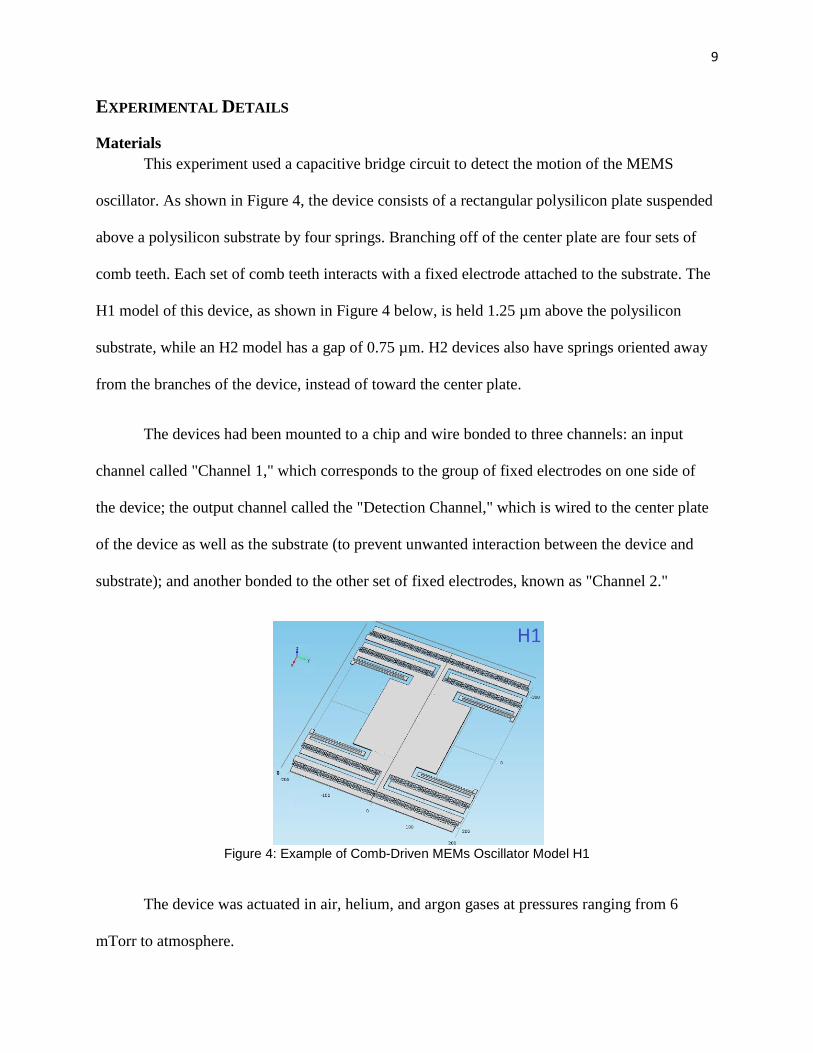
This experiment used a capacitive bridge circuit to detect the motion of the MEMS

oscillator. As shown in Figure 4, the device consists of a rectangular polysilicon plate suspended

above a polysilicon substrate by four springs. Branching off of the center plate are four sets of

comb teeth. Each set of comb teeth interacts with a fixed electrode attached to the substrate. The

H1 model of this device, as shown in Figure 4 below, is held 1.25 µm above the polysilicon

substrate, while an H2 model has a gap of 0.75 µm. H2 devices also have springs oriented away

from the branches of the device, instead of toward the center plate.

The devices had been mounted to a chip and wire bonded to three channels: an input

channel called "Channel 1," which corresponds to the group of fixed electrodes on one side of

the device; the output channel called the "Detection Channel," which is wired to the center plate

of the device as well as the substrate (to prevent unwanted interaction between the device and

substrate); and another bonded to the other set of fixed electrodes, known as "Channel 2."

Figure 4: Example of Comb-Driven MEMs Oscillator Model H1

The device was actuated in air, helium, and argon gases at pressures ranging from 6

mTorr to atmosphere.

10

Instruments

The capacitive bridge scheme shown in Figure 5 was used to detect the output of the

MEMS device. A Gertsch AC Radio Standard Ratio Transformer balanced the bridge in relation

to the two capacitive groups of comb teeth on either side of the device. The device was driven by

a homemade DC voltage source and a high frequency AC voltage source. A low-frequency

voltage, produced by a HP 33120A Voltage source, was added to the circuit via a Mini-Circuits

aplitter after passing through an 1:1 isolation transformer. This provided an excitation voltage

for the MEMS, at a variable frequency that, through was controlled through LabView to

perform frequency sweeps about the resonant frequencies of the device. The EG&G Instruments

7265 DSP lock-in amplifier provided a high frequency voltage and, via an internal sync with the

high frequency signal it produced, acted as a lock-in amplifier to detect the high frequency

output of the device. A SR530 Lock-in acted as a demodulator for the low frequency signal, and

isolated the resonance of the device. Before being demodulated by the lock-in amplifiers, the

signal from the device was amplified by a homemade low noise charge amplifier.

Figure 5: Schematic Diagram of the Measurement Circuit

11

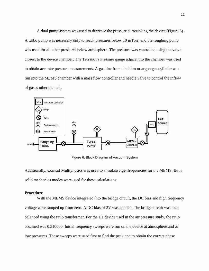
A dual pump system was used to decrease the pressure surrounding the device (Figure 6).

A turbo pump was necessary only to reach pressures below 10 mTorr, and the roughing pump

was used for all other pressures below atmosphere. The pressure was controlled using the valve

closest to the device chamber. The Terranova Pressure gauge adjacent to the chamber was used

to obtain accurate pressure measurements. A gas line from a helium or argon gas cylinder was

run into the MEMS chamber with a mass flow controller and needle valve to control the inflow

of gases other than air.

Figure 6: Block Diagram of Vacuum System

Additionally, Comsol Multiphysics was used to simulate eigenfrequencies for the MEMS. Both

solid mechanics modes were used for these calculations.

Procedure

With the MEMS device integrated into the bridge circuit, the DC bias and high frequency

voltage were ramped up from zero. A DC bias of 2V was applied. The bridge circuit was then

balanced using the ratio transformer. For the H1 device used in the air pressure study, the ratio

obtained was 0.510000. Initial frequency sweeps were run on the device at atmosphere and at

low pressures. These sweeps were used first to find the peak and to obtain the correct phase

12

setting for the low frequency lock-in amplifier. The shear mode peak was found by scanning

with a wide radius of 10 kHz around 26 kHz, since previous simulations and frequency sweeps

on other H1 devices had found that shear mode peaks usually occurred around this frequency.4 A

peak was found around 22 kHz, and was then briefly studied at a pressure of approximately

6mTorr. At this pressure it was found through use of manual phase adjustments and the analysis

of a Matlab parabolic fit program (pxlorentzfit.m) that the proper low frequency lock-in phase

for this device was +19.0°. The settings used for the rest of the circuit are shown in Table 1,

below.

Ratio Transformer

High Frequency Lock-In

Ratio 0.510000 Sensitivity 100mV

Resulting Voltage Drop

~0.27mV Time

Constant 10us

Low Frequency Lock-In High Frequency Source

Sensitivity 20mV Frequency 180KHz

Phase +19° Vrms 0.500000V

Time Constant

1 sec

Table 1: Typical System Settings

For air measurements at atmospheric pressure, the device was isolated from the BOC

Edwards rough and turbo pumps via a channel that went straight to atmosphere. For air

measurements at lower pressures, the chamber was brought to pressures down to 10mTorr by the

rough pump. The pressure was carefully controlled with the valve closest to the device chamber.

To reach pressures below 10mTorr, the chamber was pumped down to 10mTorr by the rough

pump, and then pumped down further with the turbo pump.

Once the desired pressure and system settings were reached, a frequency sweep was run

on the device. A long frequency sweep between 10 kHz and 30 kHz could be used to find the

13

rough position of the resonance peaks of the device. For the H1 device studied, it was found that

there was a shear resonance peak at approximately 22.1 kHz. In air, this peak was characterized

at 27 distinct pressures from 6mTorr to atmosphere. In helium, only 13 pressures from 6.5mTorr

to 5 Torr were studied due to the limitations of the Terranova pressure gauge. In argon, pressures

below 750mT could not be studied due to excessive air leaking into the device chamber. Each

sweep used was given a frequency range around the peak that was approximately five times the

width of the peak at half maximum. Good peak resolution was found when 200 data points were

taken per sweep. Each peak was analyzed in a MatLab program (pxlorentzfit.m) that fitted the

peak. From this program we were able to obtain useful information about the resonance,

including the amplitude, width, resonant frequency, quality factor, and phase shifting.

Each peak at each pressure was swept four times in two round-trips of frequency sweeps.

This enabled us to establish whether the peaks were exhibiting hysteresis. If this were the case,

the resonant frequencies of the upward sweeps and downward sweeps would be noticeably

different. Also, at pressures from 2 Torr to atmosphere, the excitation voltage (low frequency

voltage) was gradually increased so as to maintain a good signal to noise ratio. The highest

excitation, used at atmospheric pressure, was 5V. The lowest used in low vacuum was 0.5V.

RESULTS AND DISCUSSION

Simulations

Experimentally, throughout the studies on the various comb-driven MEMS devices

available to study, two peaks were found per device. One very sharp peak was usually observed

between 13 kHz, 16 kHz, and one somewhat broader peak was observed between 21KHz and

27KHz. With the aid of COMSOL Multiphysics simulation, the types of resonances occurring at

these frequencies can be identified.

14

Six eigenmodes were identified in our simulation for each device. However, only two of

these eigenmodes are reasonable actuations of the device. The medium in which the device

actuates is uniform, and the voltage applied to the fixed electrodes is uniformly distributed across

the comb electrodes. Therefore, any actuation that involves either twisting or bowing the device

or pivoting the device around any axis not parallel to the electrodes is not feasible (the electrode

axis is the y-axis in these images).

Figure 7 shows the device actuation for an H1 device. The color scale represents the

amount of vertical displacement from its equilibrium position (shown by the black outlines). Red

represents maximum device displacement, while blue represents minimum displacement. In

eigenmode A of Figure 7 we see that the comb teeth adjacent to the plate are bowed; the internal

combs are bowed downwards (negative z-direction) and the external combs are bowed upwards

(positive z-direction). Therefore, this cannot be easily excited by our actuation scheme. In

eigenmodes C, E, and F the device is pivoting on the x-axis, out of alignment with the fixed

electrodes, so they are also not possible. Eigenmode B, shows the device pivoting along the y-

axis only, with no evidence of bowing or twisting. Thus this eigenmode, at 15838.5 Hz, is

accepted as the pivot mode of the device. The eigenmode D, the shear mode, actuates at 25536.0

Hz actuates in the x-direction, in plane with the fixed electrodes.

The pivot mode of the device occurs due to an effect known as 'levitation.' Due to the

conductivity of the doped polysilicon, an image charge can build up on the substrate under the

device.10

This charge will repel the plate. Since an AC voltage causes this charge on one side of

the device only, the plate will pivot back and forth from the substrate on the side that the bias is

applied to.10

15

Figure 8 shows the eigenmodes of the H2 MEMs device. In these images, red represents

minimum displacement, while blue represents maximum displacement. Eigenmodes D and E

exhibit twisting along the x-axis, and modes B and F show the device bowing out of alignment

with the fixed electrodes. Eigenmodes A and C are the only modes that predict reasonable

actuation of the device. Eigenmode A pivots the device at 13812.3 Hz, and Eigenmode C, at

28432.7 Hz, is its shear mode. It was then concluded that the resonance peaks found between 13

kHz and 16 kHz were pivot resonant modes, and the peaks between 21 kHz and 27 kHz were the

shear resonant modes of the devices.

16

A B

C D

E F

Figure 7: Surface Displacement of Six Eigenmodes Simulated by COMSOL Multiphysics for an H1 Device. Red indicates maximum displacement from equilibrium, while blue represents minimum

displacement.

17

A B

C D

E F Figure 8: Surface Displacement of Six Eigenmodes Simulated by COMSOL Multiphysics for an H2 Device. Blue represents maximum displacement from the device's equilibrium position, while red

represents minimum displacement.

18

Air Pressure Study

As the air pressure study was performed, the resonant frequency, peak width, and quality

factor for each of the 27 resonant peaks were recorded and graphed. The peak width was

considered the width of the resonance peaks at half of the maximum amplitude of the peak, full

width half maximum (FWHM). It can be seen from Figure 9 that this value increased with

increasing pressure. Between approximately 100 mTorr and 75 Torr the width increased

significantly with pressure, with a proportionality of the pressure raised to a power of

approximately 0.75. Above 75 Torr and below 100 mTorr, the rate at which the width increased

with pressure decreased dramatically.

Theoretically, at low pressures it would have been expected that there should be no

change in peak width with change in pressure, as the extremely low mean free path of the gas at

this pressure should almost prevent it from interacting with the device, allowing it to actuate at

purely its intrinsic resonance response. As the pressure increases, the surrounding medium

interacts increasingly with the device, broadening the resonance peak. At high pressures, it was

expected that the increase in peak width with pressure would decrease, as the surrounding air

becomes more viscous and provides significant amounts of damping.

19

Figure 9: Air Pressure Dependence of Peak Width for H1 Device

From previous works, it was expected that the resonant frequency of the device would

remain constant up to approximately 100 Torr, 4 and then dramatically decrease due to mass

loading of the device due to high damping from the air. Our study did not show this result,

though the amount of standard deviation in results at around 100 Torr make it difficult to exclude

the possibility of mass loading at higher pressures. While it can be seen that the amount of

deviation in our resonance frequencies was only about 30 Hz at atmosphere ( approximately

0.14% of 22147 Hz, the mean resonant frequency), this deviation still makes comparison of this

result to previous pressures difficult, since all previous standard deviations are approximately

half this value or less.

It can be seen from Figure 10 that the amount of standard deviation in the error increased

with increasing pressure. It was expected that this was due to increasing amounts of hysteresis in

the up- and down-ramped frequency sweeps. At atmosphere this was effect most apparant, with

the resonant frequencies of the up-ramped peaks being approximately 22160Hz, and the

frequencies of the down sweeps approximately 22131Hz. When this effect was observed we

attempted to correct it by increasing the sweep time (from 1.750s to 3s), or amount of time that

20

the low frequency source took to "settle" to a given frequency; and by increasing the time

constant used by the low frequency lock-in (from 1s to 3s), or the amount of time over which the

average amplitude of the output was determined. This should have increased the likelihood that

up and down sweeps would obtain more similar values for the amplitude of the peak at a given

frequency and decrease hysteresis. However, these changes seemed to have little effect, and

since the percent error was still below 1%, the original data was kept. Still, it is possible, that an

improper time constant and sweep time was the source of this error at higher pressures.

Figure 10: Air Pressure Dependence of Resonant Frequency for H1 Device

The quality factor (shown in Figure 11), calculated with the fitting program in MatLab,

was equal to the ratio between the resonant frequency and FWHM. Since the resonant frequency

remained between approximately 22131 and 22168Hz throughout the study, a maximum

deviation of only 37Hz, the change in quality factor was mostly dependent on the peak width.

It can be seen that the trends in the graph of the quality factor are very similar to the

inverse of the trends in the peak width graph; at decreasingly low pressures below 0.1Torr, the

quality factor asymptotically approaches a high value of approximately 9,000 due to less gas-

21

device interaction, and the Q-factor begins decreasing much more slowly at high pressures due to

mass loading. Between 100mTorr and 75Torr, the quality factor is proportional to P0.75

.

Figure 11: Air Pressure Dependence of Quality Factor for H1 Device

Helium Pressure Study

A pressure study of the H1 device in helium gas was performed from 5 Torr down to 6.5

mTorr for a total of 13 different pressures. The FWHM, resonant frequency, and quality factor

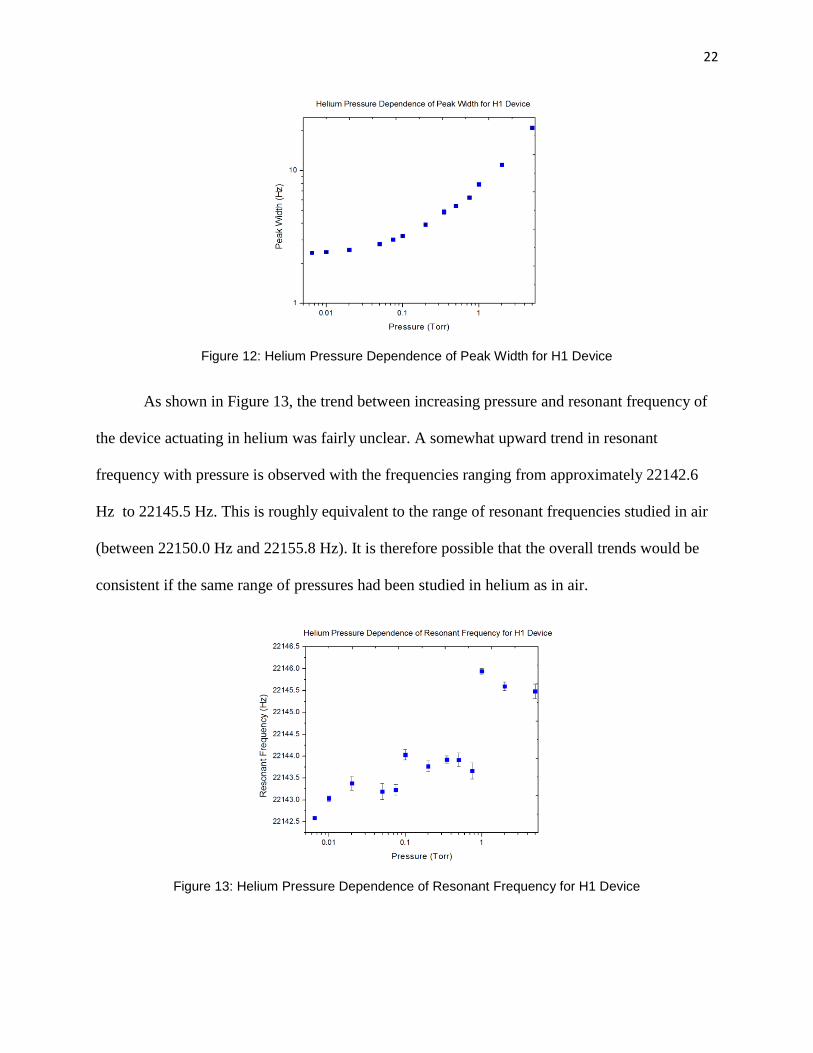
were recorded for each pressure. Figure 12 shows the relationship between peak width and

increasing pressure. At low pressures between 6.5 and 100 mTorr, it can be seen that the peak

width changed only slightly. At pressures above 100mTorr, the pressure is much more dependent

on the helium pressure. In this region of the graph, the width is proportional P0.5

.

22

Figure 12: Helium Pressure Dependence of Peak Width for H1 Device

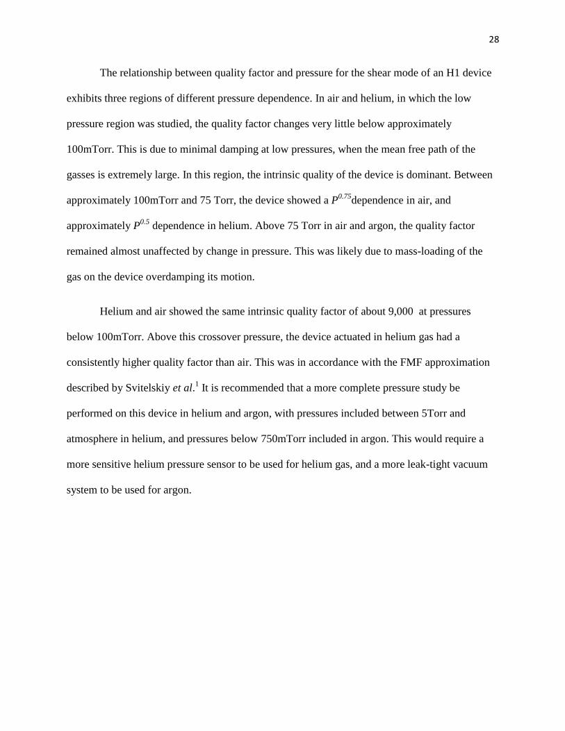
As shown in Figure 13, the trend between increasing pressure and resonant frequency of

the device actuating in helium was fairly unclear. A somewhat upward trend in resonant

frequency with pressure is observed with the frequencies ranging from approximately 22142.6

Hz to 22145.5 Hz. This is roughly equivalent to the range of resonant frequencies studied in air

(between 22150.0 Hz and 22155.8 Hz). It is therefore possible that the overall trends would be

consistent if the same range of pressures had been studied in helium as in air.

Figure 13: Helium Pressure Dependence of Resonant Frequency for H1 Device

23

The quality factor of the device at the pressures studied also showed a similar trend to the

study done in air (Figure 12). Below a pressure of approximately 100mTorr, the quality factor

changes very little with pressure, but above 100mTorr the quality factor begins decreasing with

pressure.

Figure 14: Helium Pressure Dependence of Quality Factor H1 Device

When the quality factor versus pressure study in helium is compared to that in air (Figure

14) the quality factors in both studies are approximately equal in the same low viscosity regime

below 100mTorr. Above 100mTorr, the helium study showed a consistently greater quality

factor than was found in air. In this region, the quality factor was proportional to P-0.5

.

Argon Pressure Study

A pressure study of an H1 device was done in Argon at 15 different pressures between

750mTorr and atmosphere (760Torr). Lower pressures could not be studied accurately due to air

leaks into the device chamber that significantly increased the quality factor. Figure 15 below

shows the relationship between peak width and pressure for the device actuated in argon. Peak

widths of the resonant peak above 100Torr show only slight increase with pressure due to the

24

mass loading of Argon onto the device. Below 100mTorr, the width increases proportionally to

the P0.8

.

Figure 15: Argon Pressure Dependence of Peak Width for H1 Device

The change in resonant frequency of the device with increasing pressure is reminiscent of

the trend at high pressures for the device in air. As shown in Figure 16, the resonant frequency

again increases with pressure above 100Torr, and decreases at pressures near atmosphere, likely

because of mass loading on the device. As in air, the device showed hysteresis at high pressures.

As before, these differences in up and down frequency sweeps of the device were not remedied

by increasing the low-frequency time constant and sweep time, so the averages of the up- and

down-ramped frequencies were used in this analysis.

25

Figure 16: Argon Pressure Dependence of Resonant Frequency for an H1 Device

In Figure 17, the effect of increasing argon pressure on the quality factor of the device shows a

similar relationship as the effect of increasing air pressure. Again, the quality factor decreases

logarithmically up to approximately 100Torr, and then shows little change with increasing

pressure. The quality factors below 100Torr show P0.8

dependence.

Figure 17: Argon Pressure Dependence of Quality Factor for an H1 Device

Comparison of Air, Helium, and Argon Quality Factors

26

Figure 18: Comparison of Air, Helium, and Argon Pressure Dependences of Quality Factor for H1 Device

According to Svitelskiy et al.1 the quality factor of a resonating MEMs device at low and

linear regime pressures can be calculated using a "free molecular flow" or FMF approximation.1

This model states that at pressures below the high-viscosity regime (which in our study begins at

approximately 100Torr) and above the low-viscosity regime (which in our study is below

100mTorr) the Q (in this region defined as QFMF) depends on "momentum exchange" with the

molecules of the surrounding medium.1 The overall Q can be modeled by the following equation:

At low-viscosity pressures the 1/QFMF of the device should be purely the intrinsic Q.1

This is shown in Figure 18, as the almost horizontal portion of the graph below 100mTorr. At

these pressures there is little to no difference in the Q of the device in air and in helium. In the

FMF regime, QFMF is also prominent.

27

QFMF, as shown above, is dependent on the angular frequency of the device, as well as C, a

constant value dependent on the mass and dimensions of the device, ρf, the fluid mass density of

the surrounding medium, and U, the rms speed of the gas molecules. 1

As one can see in the equation above, U is dependent on temperature (T), molar mass (M) and

the gas constant R. The fluid mass density can also be derived from the ideal gas law:

Therefore, at a given pressure, the variable determining the difference between QFMF for

helium and QFMF for air is the molar mass. This value is considerably greater for air; 29g/mol,

compared to approximately 4g/mol for helium and 40g/mol for argon. Since U increases with

lower molar mass, and QFMF decreases with increasing U. QFMF in argon will be greater than in

air. The quality factor found for the device in helium gas would be expected to be less than the

intrinsic quality factor of the device, leading to a higher overall quality factor in helium and

lower overall quality factor in argon as compared to air.

CONCLUSION

COMSOL Multiphysics simulations predicted pivot mode frequency at 15838.5 Hz and

13812.3 Hz for H1 and H2 devices, respectively. An additional shear mode was identified at

25536.0 Hz for an H1 device and 28432.7 Hz for an H2 device. This enabled us to identify the

peak we studied at approximately 22100 Hz for an H1 device as a shear mode peak.

28

The relationship between quality factor and pressure for the shear mode of an H1 device

exhibits three regions of different pressure dependence. In air and helium, in which the low

pressure region was studied, the quality factor changes very little below approximately

100mTorr. This is due to minimal damping at low pressures, when the mean free path of the

gasses is extremely large. In this region, the intrinsic quality of the device is dominant. Between

approximately 100mTorr and 75 Torr, the device showed a P0.75

dependence in air, and

approximately P0.5

dependence in helium. Above 75 Torr in air and argon, the quality factor

remained almost unaffected by change in pressure. This was likely due to mass-loading of the

gas on the device overdamping its motion.

Helium and air showed the same intrinsic quality factor of about 9,000 at pressures

below 100mTorr. Above this crossover pressure, the device actuated in helium gas had a

consistently higher quality factor than air. This was in accordance with the FMF approximation

described by Svitelskiy et al.1 It is recommended that a more complete pressure study be

performed on this device in helium and argon, with pressures included between 5Torr and

atmosphere in helium, and pressures below 750mTorr included in argon. This would require a

more sensitive helium pressure sensor to be used for helium gas, and a more leak-tight vacuum

system to be used for argon.

29

ACKNOWLEDGEMENTS

Sincere thanks to Dr. Yoonseok Lee of the University of Florida Department of Physics

for providing me the opportunity to experience and learn from the frustrations and rewards of

research in his lab this summer. Thank you also to Miguel Gonzalez, Josh Bauer, and Erik

Garcell for the valuable knowledge, advice, and support that they provided throughout this

program. This work was supported by the National Science Foundation via Grants DMR-

9820518, DMR-0139579, and DMR-0552726, as well as jointly supported by the National

Science Foundation and the Department of Defense under Grant DMR-0851707.

30

REFERENCES

1 O. Svitelskiy, V. Sauer, N. Liu, K. Cheng, E. Finley, M. R. Freeman, and W. K. Hiebert.

Phys.Rev. Lett. 103, 244501 (2009).

2 Kaajakari, Ville. Practical MEMs. Las Vegas: Small Gear, 2009. Print.

3 M. Zougagh and A. Rios. Analyst, 134, 1274-1290 (2009).

4 Miguel A. Gonzalez. Development and Application of MEMs Devices for the Study of Liquid

3He. PhD Thesis. University of Florida, 2012.

5 Nave, C. R. "Liquid Helium." HyperPhysics. Georgia State University, 2012. Web. 23 July

2012. <http://hyperphysics.phy-astr.gsu.edu/hbase/hph.html>.

6 C. Um, H. Oh, J. Cho, C. Jun, and T. F. George. J. KPS. 42, 437-56 (2003).

7 K. Kono. Physica 4, 110 (2011).

8 J. C. Davis, A. Amar, J. P. Pekola, R. E. Packard, Phys. Rev. Lett. 60, 4 (1988).

9 Fortner, Michael R. "Duffing Oscillator." Physics 500 Lecture. Northern Illinois University,

DeKalb. 20 June 2012. Lecture.

10

W. C. Tang, Solid-State Sensor and Actuator Workshop, Technical Digest., IEEE 4, 23 (1990).