preliminary covariances obtained with conrad/gromacs · pdf filepreliminary covariances...

PRELIMINARY COVARIANCES OBTAINED

WITH CONRAD/GROMACS FOR H(H20)

10-11 May 2016

Gilles NOGUERE, Juan Pablo SCOTTA, Jose Ignacio MARQUEZ DAMIAN,

Pascal ARCHIER, Cyrille DE SAINT JEAN, Pierre LECONTE, Guillaume

TRUCHET, Oscar CABELLOS, I. HILL, Olivier LERAY, Dimitri ROCHMAN

9 MAI 2016

| PAGE 2

Outlines

Two main objectives:

• Create covariance matrix between the LEAPR parameters for JEFF-3.1.1

• Create covariance matrix between the GROMACS parameters for the CAB model

Propagation of the TSL uncertainties to integral calculations by using:

• Direct perturbation of the model parameters

• Random S(,) tables (TMC calculation)

• Sensitivity calculations

| PAGE 3

Covariance matrix between the LEAPR model

The first step was to determine the covariance matrix between the LEAPR parameters

2 main parameters were identified:

• The energy bin uses to reconstruct

the phonon spectrum

• The weight wt of the translational

vibration mode

Phonon spectrum H(H20)

https://www.oecd-nea.org/science/wpec/sg42/




15.2%

3.8%

3.1%

10.6%

7.2%

1.3%

| PAGE 4

Propagation of the TSL uncertainties

H1-Elastic Thermal uncer (%)=TMC/Sens 10-3

TMC . vs. H1-Elastic Scattering Thermal Sensitivity Coefficient

Results obtained from

random TSL files

(NSE 172, 287, 299, 2012)

15.2%

3.8%

3.1%

10.6%

7.2%

1.3%

| PAGE 5

Propagation of the TSL uncertainties

H1-Elastic Thermal uncer (%)=TMC/Sens 10-3

TMC . vs. H1-Elastic Scattering Thermal Sensitivity Coefficient

Preliminary set of

selected

benchmarks

| PAGE 6

Propagation of the TSL uncertainties of JEFF-3.1.1

Benchmarks EALF

(eV)

EAFG

(eV)

TMC Direct perturbation of

the LEAPR parameters

SERPENT MCNP TRIPOLI4

HEU-SOL-THERM-042-001 0.0320 0.0388 35 pcm

LEU-SOL-THERM-004-001 0.0421 0.0735 53 pcm 79 pcm

PU-SOL-THERM-012-014 0.0783 0.1440 132 pcm

PU-SOL-THERM-001-001 0.0885 0.1660 157 pcm 160 pcm 145 pcm

LEU-COMP-THERM-007-001 0.2870 0.5910 110 pcm

MISTRAL-2 (MOX) - - 199 pcm

Random files can be found in the WPEC/SG42 web site


Cf. presentation of Juan Pablo Scotta on MISTRAL-1

Low sensitivity to H(H2O)

Excellent agreement between the different codes and methods




| PAGE 7

Covariance matrix between the GROMACS parameters

Water potential TIP4P/2005f

CAB model for water

Zero Variance Penalty model in CONRAD

Contributions GROMACS functions Parameters

Lennard-Jones potential

sigma

epsilon

Electrostatic interaction e

Morse potential

b

D

Beta

Harmonic angle potential theta0

k

« dummy » atom a=b

GROMACS parameters for water

GROMACS parameters for water

Prior values, variances and correlations

Phonon spectrum generated

with the GROMACS results

Discrete oscillators are

replaced by a continuuous

spectrum

Diffusion constant

(translational mode) is

deduced from the

GROMACS results

(Mx’)-1=Mx

-1+GtC-1G

X’=X0+Mx’GtC-1(Y-Yth(X0))

0XXj

ith

ijx

yG

for i = 1,m and j = 1,n

iteration 1

with Mx = diag(var(x01) … var(x0n))

(Mx’’)-1=Mx

-1+GtC-1G

X’’=X’+Mx’’GtC-1(Y-Yth(X’))

'XXj

ith

ijx

yG

for i = 1,m and j = 1,n

iteration 2

iteration 3 …

Linear least-squares : « best » estimate of the GROMACS parameters are found iteratively

by solving the following generic equations

and

with

Fitting model of CONRAD

| PAGE 10

Such a fitting model was not designed to account for uncertainties of “systematic” origin.

This problem was solved in CONRAD by introducing marginalization techniques

These methods account for uncertainties of the “nuisance” and “latent” model parameters

Fitting model of CONRAD

| PAGE 11

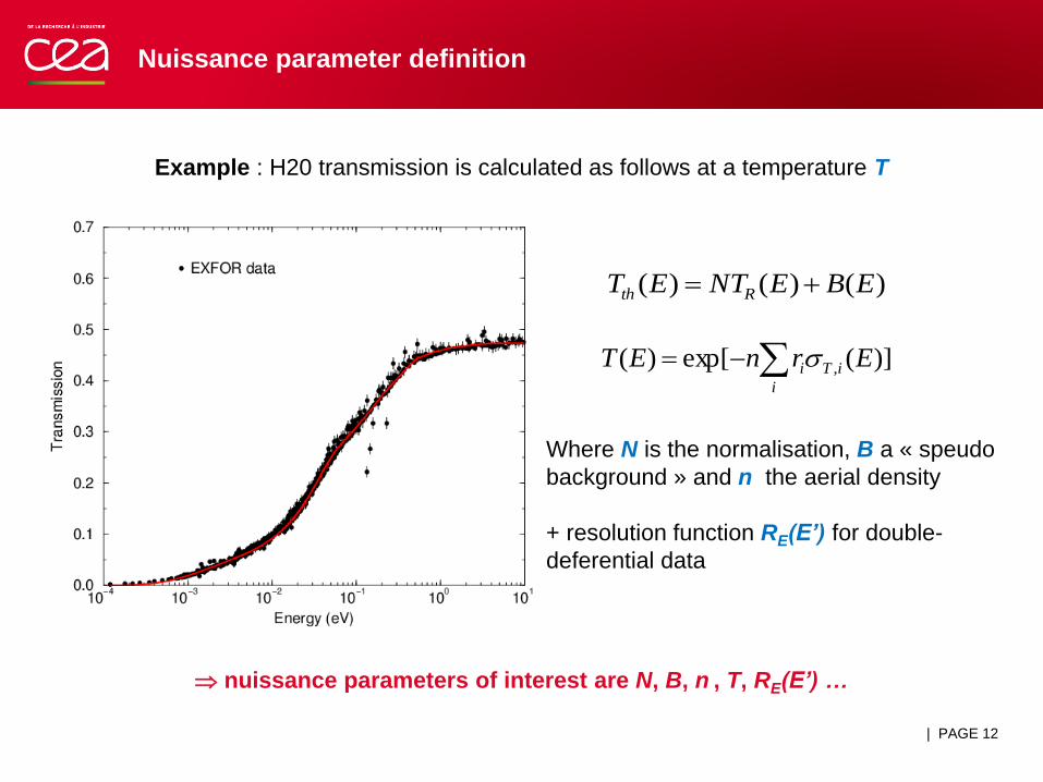
])(exp[)( ,i

iTi ErnET

Example : H20 transmission is calculated as follows at a temperature T

)()()( EBENTET Rth

Where N is the normalisation, B a « speudo

background » and n the aerial density

+ resolution function RE(E’) for double-

deferential data

Nuissance parameter definition

nuissance parameters of interest are N, B, n , T, RE(E’) …

| PAGE 12

Latent model parameter definition

Latent variables (as opposed to observable variables which can be fitted on the

experimental data) may define redundant parameters or hidden variables that cannot be

observed directly. This term reflects the fact that such variables are really there, but they

cannot be observed or measured for practical reasons.

Example : contributions of O(H2O) and free atom cross sections of H and O

H(H2O)

O(H2O)*

H

O

uncertainties are

unknown for the

moment

*O(H20) from Jose Ignacio Marquez Damian






Example : contributions of O(H2O) and free atom cross sections of H and O

References H O

IKE model (JEFF-3.1.1) 20.478 b 3.761

Atlas of Neutron

Resonances 20.4910.014 b 3.7610.006 b

STD2006 (IAEA) 20.4360.041 b

JEFFDOC-1488 20.474 0.012 b 3.761 0.005 b

0.2% 0.2%






Example : contribution of the translational weight t

In the CAB model, the translational weight is deduced from the measurements performed

by Novikov

1

22

OH

diff

OH

H

diff

Ht

m

m

m

m

m

m

a relative uncertainty of 10% is assumed in the calculations

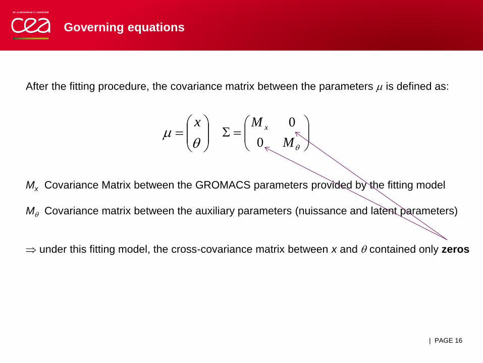
Mx Covariance Matrix between the GROMACS parameters provided by the fitting model

M Covariance matrix between the auxiliary parameters (nuissance and latent parameters)

M

M x

0

0

After the fitting procedure, the covariance matrix between the parameters is defined as:

Governing equations

under this fitting model, the cross-covariance matrix between x and contained only zeros

| PAGE 16

x

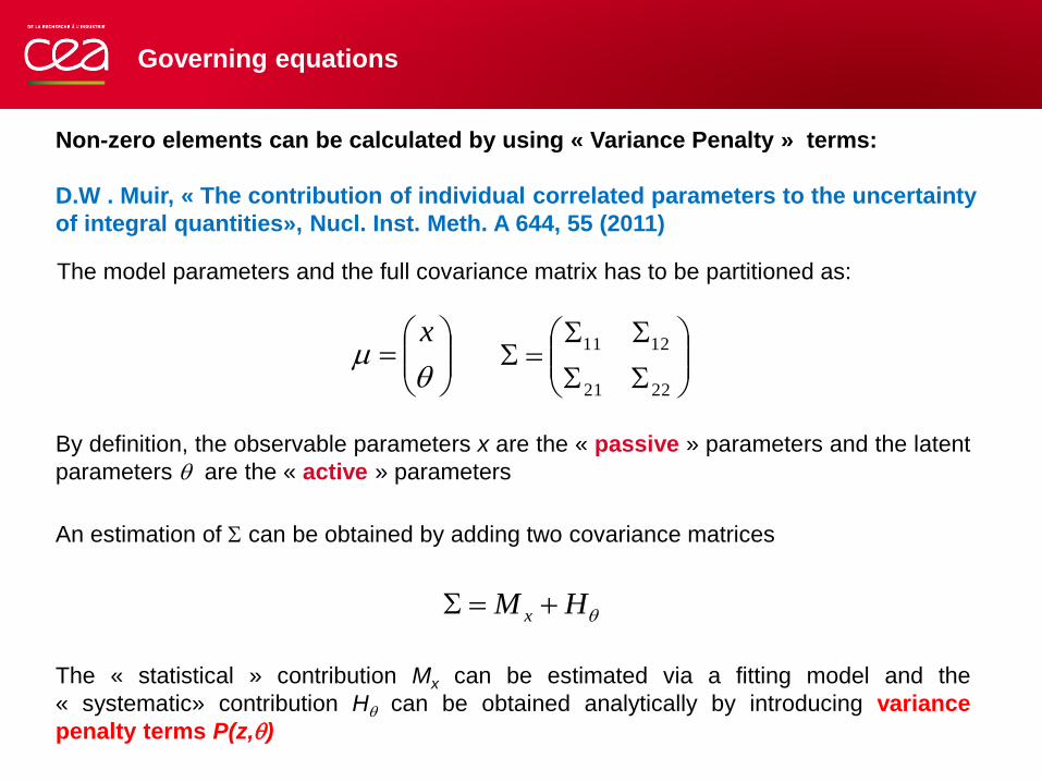
Governing equations

The model parameters and the full covariance matrix has to be partitioned as:

Non-zero elements can be calculated by using « Variance Penalty » terms:

D.W . Muir, « The contribution of individual correlated parameters to the uncertainty

of integral quantities», Nucl. Inst. Meth. A 644, 55 (2011)

2221

1211

x

By definition, the observable parameters x are the « passive » parameters and the latent

parameters are the « active » parameters

An estimation of can be obtained by adding two covariance matrices

The « statistical » contribution Mx can be estimated via a fitting model and the

« systematic» contribution H can be obtained analytically by introducing variance

penalty terms P(z,)

HM x

Governing equations

| PAGE 18

TGGHzP ),(

P(z,) is a measure of the contribution of the uncertainty of the latent and nuisance variables

to the variance of a given calculated quantity z. By definition

n

kk

n

x

z

x

z

x

z

x

z

xG

1

1

1

1

m

kk

m

zz

zz

G

1

1

1

1

The covariance matrix H has the following form

For a vector quantity z of general dimension k, the derivative matrix G=(Gx,G) of the quantity

z to the parameters x and is defined as:

MM

MMMMH

x

T

x

T

xx

,

,,

1

,

The « zero variance penalty » condition lead to

| PAGE 19

MGGGGM T

xx

T

xx

1

, )(

According to the definition of , we have

Governing equations

2221

1211 11

11

x

T

xx

TT

xx

T

xx GGGGMGGGGM

MGGGG T

xx

T

x

1

12 )(

22 = M

By using the partitioned form of G, we have

0),( ,,,

1

, TTT

xx

T

xx

T

x

T

xxx GMGGMGGMGGMMMGzP

Covariance matrix between the parameters:

• GROMACS parameters

• Experimental parameters

• LEAPR parameters

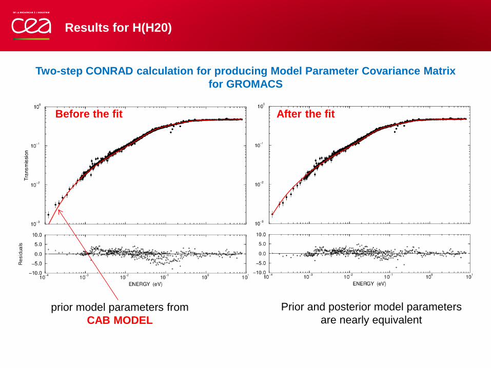
Results for H(H20)

Two-step CONRAD calculation for producing Model Parameter Covariance Matrix

for GROMACS

Before the fit After the fit

prior model parameters from

CAB MODEL

Prior and posterior model parameters

are nearly equivalent

Results for H(H20)

Two-step CONRAD calculation for producing Model Parameter Covariance Matrix

for GROMACS

After the fit

Mx

After marginalization

11

11

11

x

T

xx

TT

xx

T

xx GGGGMGGGGM

Results for H(H20)

Relative uncertainties and correlation matrix for H2O (transmission)

After the fit

After

marginalization

Results for H(H20)

Relative uncertainties and correlation matrix on S(,)

Calculated with the Model

Parameter Covariance Matrix

obtained after marginalization

How to store large covariance

matrix for S(,) ? Strange results !

To be confirmed

| PAGE 24

IDC format to store large covariance matrix

IDC : a solution to store large Resonance-Parameter Covariance Matrix

• Available in SAMMY and CONRAD to read

AGS covariance file (used at the IRMM)

• Cf. WPEC/SG-36 «Evaluation of

experimental data in the resolved

resonance region»

IDC format can be also used to store covariance matrix for S(,)

« A concise method for storing and communicating the Experimental

Covariance Matrix », N.M. Larson, ORNL/TM-2008/104, 2008

| PAGE 25

.....

.....

.....

)var(44332211

xLLLL xxxx

nn

m+1

MSSD T

diagonal matrix

Variance on S(,) from the

fitting procedure

Correlations from the fit are

neglected

Derivatives of S(,) to the

nuissance parameters

introduced in the

marginalization procedure

IDC format to store large covariance matrix

Propagation of TSL uncertainties to integral calculations

Var(z)=SDST

For a given integral quantity z, the variance is calculated as follow:

Where D is the covariance matrix for S(,) and S contains the derivatives of z to S(,)

Exemple: Sensitivity to the elastic scatering of H(H20) in PST001.1 as a function of the

incident energy and obtained with TRIPOLI4-IFP (PhD thesis G.Truchet, CEA Cadarache)

MeV energy range

Thermal cut-off energy

5.0 eV

Up-scattering

Propagation of TSL uncertainties to integral calculations

Exemple: Sensitivity to S(,) of H(H20) in PST001.1 obtained with TRIPOLI4-IFP (PhD

thesis G.Truchet, CEA Cadarache)

Zoom on the (,) region

of interest for this work

Final calculations Var(z)=SDST not yet performed !

Conclusions

Present results on TSL uncertainties

CONRAD can be use to produce Model Parameter Covariance Matrix for LEAPR

CONRAD can be use to produce Model Parameter Covariance Matrix for GROMACS

Production of large covariance matrix for S(,) is possible with the IDC formalism

TRIPOLI4-IFP can be used to propagate TSL uncertainties to integral data

Next steps

Include double-differential and mu-bar data in the fitting procedure

Generate random files for the CAB model

Finalize the propagation of the uncertainties with TRIPOLI4-IFP

Acknowledgment

Special thanks to Jose Ignacio Marquez Damian for his help on using GROMACS and for

the fruitful discussions and advices.

preliminary covariances obtained with conrad/gromacs · pdf filepreliminary covariances...

Documents