A.C. Robin

Institut UTINAM, OSU THETA, Besançon Coll. C. Reylé, S. Diakité, O. Bienaymé, J. Fernandez-Trincado, R. Mor, F. Figueras, etc.

Preliminary comparisons between a Galaxy model and Gaia DR1

1

Outline

• Introduction

• Population synthesis approach

• Preliminary star count comparisons : DR1 tests for completeness

• RAVE+TGAS synergy: Constraints on the disc kinematics

• Perspectives

2

Gaia

• Revisiting our understanding of Galaxy formation and evolution

• 6D space explored for hundreds of million stars, 4D for 2 billion stars

Gaia challenge : Find efficient methods to analyse and interpret data in terms of Galaxy evolution & dynamics

• Estimates for the density of detected stars (GUMS10)

• artiste’s view of the MW from top

• => Gaia will revolutionize this view (at least for a quarter of the Galactic plane)

Population Synthesis Modelling

• Population synthesis approach: many parameters but more understanding

• Statistical treatment : no individual distances and ages, but for groups of stars

• Link between scenarios and observations

• Increasing complexity (start simple…)

• Confronted to many observables : magnitudes, colors (many bands), proper motions, radial velocities, Teff, logg, [Fe/H],[alpha/Fe], asterosismic paramaters in the future

6

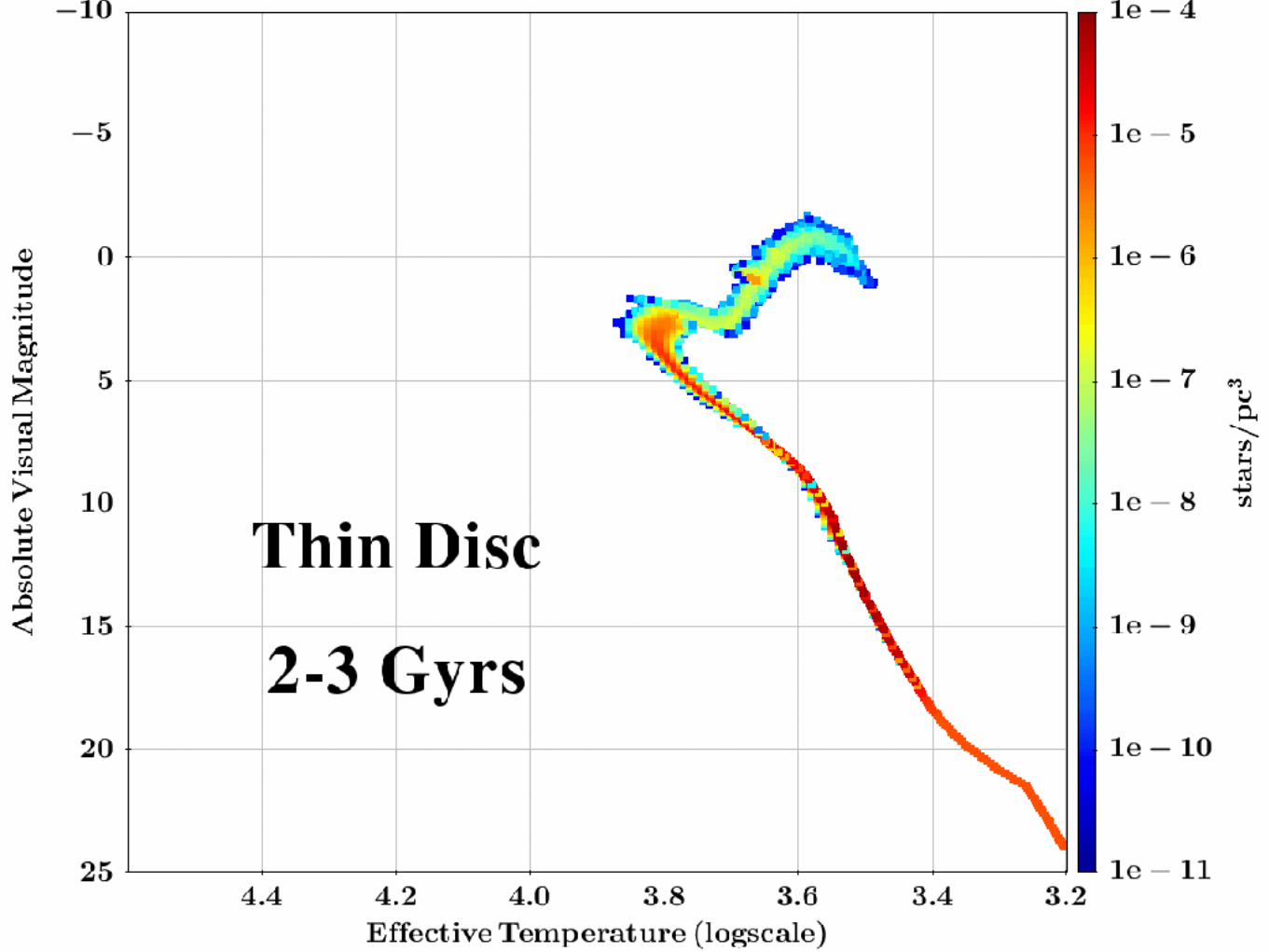
Mor et al, 2016

ϕ(Teff, logg) for a

thin disc decreasing SFR over 10 Gyr

New Besançon Galaxy model

Czekaj et al, 2014Robin et al, 2014

Bienaymé et al 2015Lagarde et al 2017

Binarity included

3D Extinction model (Mashall et al, 2006)

Comparison to bright star counts

Tycho-2: VT < 11.5 BGM

Mor et al, 2016

=> Good at |b|>10° But Need for a better extinction model (low distances) at |b|<10°

Comparisons with DR1

0,

120,

240,

-60, -60,

0, 0,

60, 60,

-1.0-0.8-0.6-0.4-0.200.20.40.60.81.0

RelDiff12

0,

120,

240,

-60, -60,

0, 0,

60, 60,

-1.0-0.8-0.6-0.4-0.200.20.40.60.81.0

RelDiff13

0,

120,

240,

-60, -60,

0, 0,

60, 60,

-1.0-0.8-0.6-0.4-0.200.20.40.60.81.0

RelDiff14

0,

120,

240,

-60, -60,

0, 0,

60, 60,

-1.0-0.8-0.6-0.4-0.200.20.40.60.81.0

RelDiff15

0,

120,

240,

-60, -60,

0, 0,

60, 60,

-1.0-0.8-0.6-0.4-0.200.20.40.60.81.0

RelDiff16

0,

120,

240,

-60, -60,

0, 0,

60, 60,

-1.0-0.8-0.6-0.4-0.200.20.40.60.81.0

RelDiff17

0,

120,

240,

-60, -60,

0, 0,

60, 60,

-1.0-0.8-0.6-0.4-0.200.20.40.60.81.0

RelDiff18

0,

120,

240,

-60, -60,

0, 0,

60, 60,

-1.0-0.8-0.6-0.4-0.200.20.40.60.81.0

RelDiff19

Relative differences between Gaia-DR1 and BGM (GOG18) in magnitude bins

12<G<13 13<G<14 14<G<15 15<G<16 16<G<17 17<G<18 18<G<19 19<G<20

Tests for completeness

Arenou et al, 2017, A&A 599, A50

Disc kinematics: RAVE + TGAS

• Complementarity between RAVE & Gaia-DR1 (TGAS): radial velocities + proper motions

• RAVE based on Tycho-2 : I<12

• TGAS p.m. 1st epoch from Tycho-2

• RAVE simple selection function (random subsets)

• However TGAS incomplete at VT>10.5

19

RAVE selection test

• BGM simulation applying RAVE selection function on I magnitude

0.0

0.2

0.4

0.6

0.8

1.0

1.2

1.4

x104

3000 3500 4000 4500 5000 5500 6000 6500 7000 7500 8000 8500 9000TeffS

Count

0.00.1

0.2

0.3

0.4

0.5

0.6

0.7

0.8

0.9

1.0x104

0.0 0.5 1.0 1.5 2.0 2.5 3.0 3.5 4.0 4.5 5.0loggS

Count0

200

400

600

800

1000

1200

1400

1600

1800

2000

9.0 9.5 10.0 10.5 11.0 11.5 12.0

Count

Resulting Teff / logg

Galactic dynamics

• To obtain self-consistent distribution functions : Determine third integral of motion.

• Approximate potential of the BGM with a Stäckel potential=> Fitting orbits to obtain the Stäckel parameters => 3rd integral

• Compute potential, vertical and radial forces self-consistently

• Describe the asymmetric drift as a function of Rgal, Zgal

Bienaymé et al 2015

150

200

250

300

350

0 5 10 15 20

V (

km

/s)

R (kpc)

Caldwell+ (1981)

Model 1

Sofue2015

Model 2

Bienaymé et al 2015Meridional projection of 3 orbits

Envelop of the orbits (analytical)

Surfaces of sectionR (kpc) 200

V

Good Stäckel approximation (<1%) for a wide Galactic range (3<Rgal<12 kpc, -6<Zgal<6 kpc)

Kinematical model

Kinematics of each star computed (in heliocentric reference frame) from

• Galactic rotation curve (from potential)

• Asymmetric drift (from potential)

• Solar motion (3 free parameters)

• Age - velocity dispersion relation (3-4 free parameters)

• Radial velocity gradients (2 free parameters)

• Vertex deviation (2 free parameters)

Mihalas (1968)

density gradient velocity disp. gradient

Older stars rotated slower than young stars and gas

Asymmetric drift

Generally assumed to be the same out of the plane, but not the case in reality (Binney et al, 2010,2012), Bienaymé et al 2015)

0

20

40

60

80

100

120

140

160

0 1 2 3 4 5 6

Vlag

km

/s

Zgal (kpc)

0

10

20

30

40

50

60

70

80

90

100

2 4 6 8 10 12

Vlag

km

/s

Rgal (kpc)

Dependency of the asymmetric drift with R and zOld thick disc

Young thick disc

Thin discs

In this self-consistent dynamical model

Kinematical constraints at the Solar neighborhood

Solar motion

Thin disc velocity dispersion as a fct of age

Thick disc velocity ellipsoid

Kinematical gradients26

• Simulating the RAVE survey selection function, radial velocities

• Gaia TGAS : accurate proper motions for the RAVE stars

• Separate stars by metallicity (4 bins) and by temperature (cool/hot)

• |b|>25° to avoid extinction problems (and complex selection function)

• Fit kinematic model for the thin and thick discs (ABC-MCMC)

Robin, Bienaymé, Reylé, Fernandez-Trincado, 2017, 2017arXiv170406274R

Solving for

Age-velocity dispersion relation in the local thin disc

0

10

20

30

40

50

0 2 4 6 8 10

SigmaW (km/s)

Age (Gyr)

Gomez et alHolmberg

Sharma+2014Bovy+2012Fit (1)Fit (2)Fit (3)

19972009

0.00

0.02

0.04

0.06

0.08

0.10

0.12

0.14

0.16

0.18

0.20

-50 -40 -30 -20 -10 0 10 20 30 40 50pmra

Nor

mal

ised

cou

nt

0.00

0.02

0.04

0.06

0.08

0.10

0.12

0.14

0.16

0.18

0.20

0.22

-50 -40 -30 -20 -10 0 10 20 30 40 50pmdec

Nor

mal

ised

cou

nt

0

1

2

3

4

5

6

7

8

9

x10-2

-150 -100 -50 0 50 100 150HRV

Nor

mal

ised

cou

nt

Vlos

pmdecpmra

Hot: solid cool: dashed

Data Model

29

0 1 2 3 4 5 6 7

-150 -100 -50 0 50 100 150 200

b<-7

0

HRV

0 5

10 15 20 25 30 35 40 45

-150 -100 -50 0 50 100 150 200HRV

0 20 40 60 80

100 120 140 160 180

-150 -100 -50 0 50 100 150 200HRV

0 10 20 30 40 50 60 70 80 90

100

-150 -100 -50 0 50 100 150 200HRV

0 0.5

1 1.5

2 2.5

3 3.5

4

-150-100 -50 0 50 100 150 200

135<

l<22

5 -7

0<b<

-40

HRV

0

5

10

15

20

25

-150 -100 -50 0 50 100 150 200HRV

0 10 20 30 40 50 60 70 80 90

-150 -100 -50 0 50 100 150 200HRV

0 5

10 15 20 25 30 35 40 45

-150 -100 -50 0 50 100 150 200HRV

0 2 4 6 8

10 12 14 16 18

-150 -100 -50 0 50 100 150 200

225<

l<31

5 -7

0<b<

-40

HRV

0 10 20 30 40 50 60 70 80

-150 -100 -50 0 50 100 150 200HRV

0 50

100 150 200 250 300

-150 -100 -50 0 50 100 150 200HRV

0 20 40 60 80

100 120

-150 -100 -50 0 50 100 150 200HRV

0 2 4 6 8

10 12 14 16 18

-150 -100 -50 0 50 100 150 200

-45<

l<13

5 -7

0<b<

-40

HRV

0 20 40 60 80

100 120

-150 -100 -50 0 50 100 150 200HRV

0 50

100 150 200 250 300 350 400 450

-150 -100 -50 0 50 100 150 200HRV

0 20 40 60 80

100 120 140 160 180

-150 -100 -50 0 50 100 150 200HRV

0

1

-150 -100 -50 0 50 100 150 200

135<

HRV

0

5

-150 -100 -50 0 50 100 150 200HRV

0 10 20

-150 -100 -50 0 50 100 150 200HRV

0 5

-150 -100 -50 0 50 100 150 200HRV

0

5

10

15

20

-150 -100 -50 0 50 100 150 200

b<-7

0

HRV

0 20 40 60 80

100 120 140

-150 -100 -50 0 50 100 150 200HRV

0 100 200 300 400 500 600

-150 -100 -50 0 50 100 150 200HRV

0 50

100 150 200 250 300 350 400

-150 -100 -50 0 50 100 150 200HRV

0 2 4 6 8

10 12 14

-150 -100 -50 0 50 100 150 200

135<

l<22

5 -7

0<b<

-40

HRV

0 10 20 30 40 50 60

-150 -100 -50 0 50 100 150 200HRV

0 50

100 150 200 250 300

-150 -100 -50 0 50 100 150 200HRV

0 20 40 60 80

100 120 140 160 180

-150 -100 -50 0 50 100 150 200HRV

0

5

10

15

20

25

-150 -100 -50 0 50 100 150 200

225<

l<31

5 -7

0<b<

-40

HRV

0 20 40 60 80

100 120 140

-150 -100 -50 0 50 100 150 200HRV

0 100 200 300 400 500 600 700

-150 -100 -50 0 50 100 150 200HRV

0 50

100 150 200 250 300 350 400 450 500

-150 -100 -50 0 50 100 150 200HRV

0 5

10 15 20 25 30 35

-150 -100 -50 0 50 100 150 200

-45<

l<13

5 -7

0<b<

-40

HRV

0 20 40 60 80

100 120 140 160 180

-150 -100 -50 0 50 100 150 200HRV

0 100 200 300 400 500 600 700 800 900

-150 -100 -50 0 50 100 150 200HRV

0 100 200 300 400 500 600 700

-150 -100 -50 0 50 100 150 200HRV

0 1

-150 -100 -50 0 50 100 150 200

135<

HRV

0 5

-150 -100 -50 0 50 100 150 200HRV

0 20 40

-150 -100 -50 0 50 100 150 200HRV

0 20

-150 -100 -50 0 50 100 150 200HRV

Cool stars

hot stars > 5200K

-1.2<[Fe/H]<-0.8 -0.8<[Fe/H]<-0.4 -0.4<[Fe/H]<0 0<[Fe/H]<0.4

-1.2<[Fe/H]<-0.8 -0.8<[Fe/H]<-0.4 -0.4<[Fe/H]<0 0<[Fe/H]<0.4

Gaia proper motions

hot stars

U V WSun

velocities 11.9 0.9 7.1

Velocity dispersions

Thick disc 10 Gyr

42±2 31±2 27±1

Thick disc 12 Gyr

80±8 57±9 62±6

31

Thick disc dynamical evolution: confirms the contraction between 12 Gyr and 10 Gyr, determined from the scale height and scale length (R+2014)

Solar motion

• New determination of the Solar motion

• (Uo,Vo,Wo)=(13,1,7) km/s : good agreement for U and W with literature

• Vo smaller than previous determinations

• Literature values for Vo: from 3 to 26 km/s !

Solar V velocity• Results depend on

• tracer used (…UCAC4 => TGAS)

• kinematical models (including asymmetric drift f(z) or not,…)

• rotation curve / Sun - Galactic centre distance

• local/non local determination

• Method for fitting

• use of distances or direct observables (magnitudes, Vrad, proper motions)

• Vo uncertainty always larger than the internal accuracy of the fit

Gomez et al 1977Dehnen & Binney 1998

Schönrich & Binney (2010)

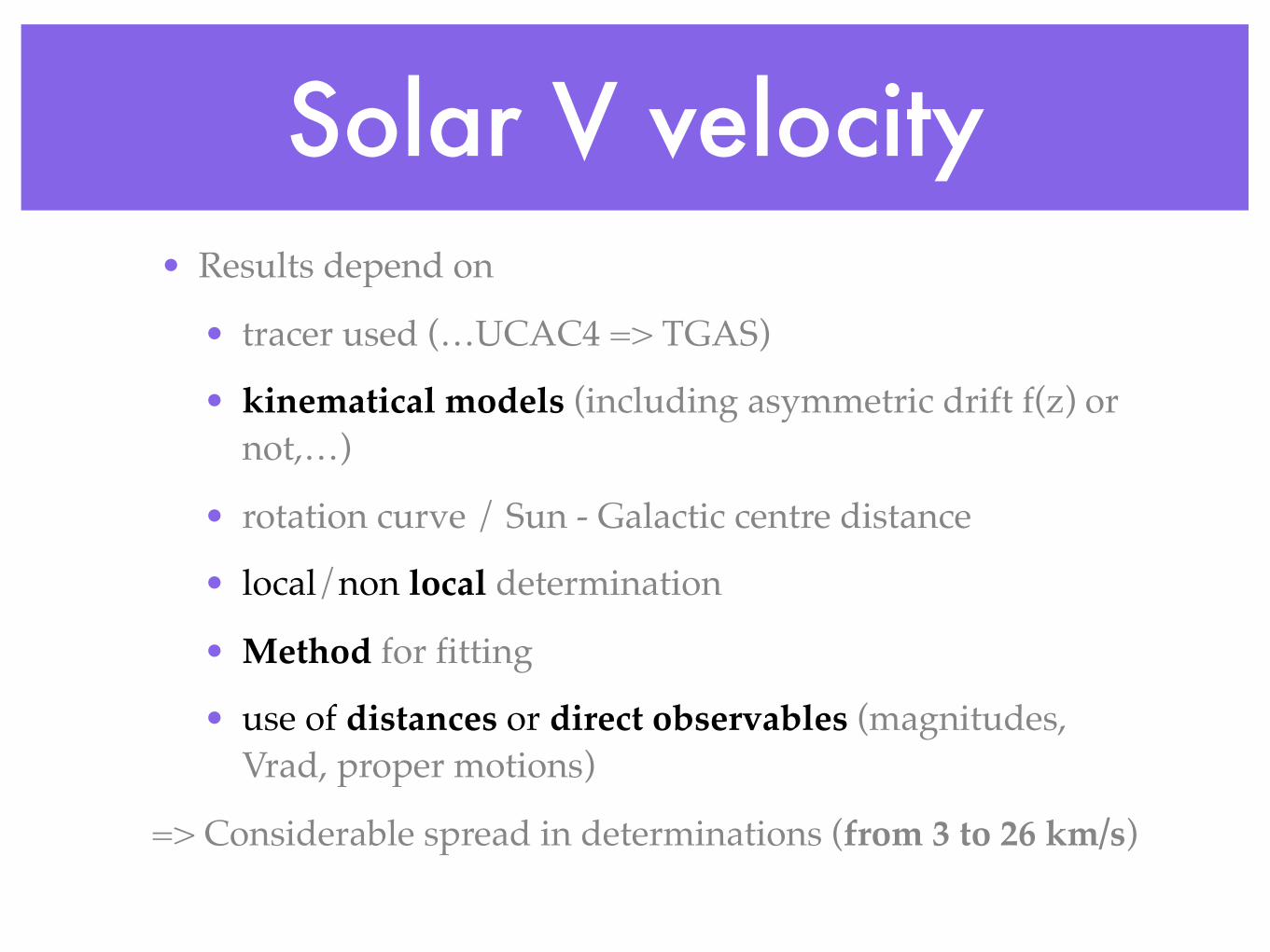
Solar V velocity• Results depend on

• tracer used (…UCAC4 => TGAS)

• kinematical models (including asymmetric drift f(z) or not,…)

• rotation curve / Sun - Galactic centre distance

• local/non local determination

• Method for fitting

• use of distances or direct observables (magnitudes, Vrad, proper motions)

=> Considerable spread in determinations (from 3 to 26 km/s)

Vo (among others)

• Dehnen & Binney (1998): from 15,000 stars Hipparcos: 5.25 ± 0.62 km/s−1

• Aumer & Binney (2009): Hipparcos re-reduction: ~5 km/s

• Binney (2010): GCS + SDSS and new dynamical model: 11 km/s

• Schönrich & Binney (2010): 12.24 ± 0.47 km/s

• Sharma et al (2014): RAVE + GCS: 7.6 km/s

Schönrich, Binnen & Dehnen, 2010

•Self-consistent dynamical models (but different)

In common:

Main differences:

•Hipparcos + GCS •Distances from

spectrophotometric parallaxes •Vo=12 km/s

•Radial velocities from RAVE •Proper motions from Gaia-TGAS •No distances assumed (space of

observables) •Vo=1km/s

Schönrich et al. 2010 This work (astroph.1704.06274)

Sharma et al 2014In common:

Main differences:

• Self-consistent dynamical models (but different) •RAVE data •In the space of observables •MCMC exploration

•Proper motions from Gaia-TGAS •Gaussian distribution fct •Vo= 1 km/s

•Proper motions from UCAC4 •Shu distribution fct • Vo= 7 km/s

This work (astroph.1704.06274) Sharma et al. 2014

kinematical radial scale length

VoSharma+2014

Summary

• New dynamical self-consistency model with a Stäckel potentiel

• A correct asymmetric drift modeling is important for determining the solar motion

• Need to be confirmed from Gaia-DR2

• Still an axisymmetric model

• Exploration of non-axisymmetries (bar) using test-particle simulations from the BGM potential (Fernandez-Trincado in preparation)

40

Perspectives• Gaia DR2 coming soon

• Extend this analysis to Gaia DR2 data, with radial velocities and proper motions

• Consider using parallaxes with good accuracies

• Combine RAVE+APOGEE+Gaia data sets => wide Galaxy portion with reliable data, new constraints on radial velocity gradients

• Improve dynamical model and explore non-axisymmetries

Improved BGM (v. 2016) available http://model2016.obs-besancon.fr and web service http://model2016.obs-besancon.fr/ws

Thanks for your attention

42