prelaunch testing of the laser - ilrs home page · 2013-07-18 · tech library kafb, nm nasa...

< c

NASA Technical Paper 1062

NASA TP 1062 c.1

'U L r

Prelaunch Testing of the Laser Geodynamic Satellite (LAGEOS)

M. W. Fitzrnaurice, P. 0. Minott, J. B. Abshire, and H. E. Rowe

OCTOBER 1977

TECH LIBRARY KAFB, NM

NASA Technical Paper 1062 0334229


M. W. Fitzmaurice, P. 0. Minott, J. B. Abshire, and H. E. Rowe Goddard Space Flight Center Greenbelt, Maryland

National Aeronautics and Space Administration

Scientific and Technical Information Office

1977

This document makes use of international metric units according to the Systeme International d’Unites (SI). In certain cases, utility requires the retention of other systems of units in addition to the SI units. The conven- tional units stated in parentheses following the computed SI equivalents are the basis of the measurements and calculations reported.

CONTENTS

Page

INTRODUCTION . . . . . . . . . . . . . . . . . . . . . . . . . . 1

TARGET SIGNATURE TESTS . . . . . . . . . . . . . . . . . . . . . 3

LIDAR CROSS-SECTION TESTS . . . . . . . . . . . . . . . . . . . . 26

SUMMARY OF TEST RESULTS . . . . . . . . . . . . . . . . . . . . 41

ACKNOWLEDGMENTS . . . . . . . . . . . . . . . . . . . . . . . . 55

REFERENCES . . . . . . . . . . . . . . . . . . . . . . . . . . . 57

APPENDIXA-ANALYSIS OF LAGEOS USING RETRO PROGRAM . . . . . . . A-1

APPENDIX B-A SECOND METHOD OF MEASURING THE RANGE CORRECTION . . . . . . . . . . . . . . . . . . . . . B-1

P R E L A U N C H T E S T I N G OF T H E L A S E R G E O D Y N A M I C S A T E L L I T E ( L A G E O S )

M:W. Fitzmaurice, P. 0. Minott, J . B. Abshire, and H. E. Rowe Goddard Space Flight Center

Greenbelt, Maryland

INTRODUCTION

The Laser Geodynamic Satellite (Lageos) was launched from the Western Test Range on May 3 , 1976, and achieved its planned orbit. Although there are several other satellites that are used as targets by ground-based laser ranging systems, this is the first satellite devoted exchsiuely to laser ranging. As such, the Lageos plays a key role in the National Aeronautics and Space Administration’s (NASA’s) Earth and Ocean Dynamics Application Program (EODAP), as well as the increasing international effort in laser measurement systems for geophysics investigations (Reference 1). Lageos is expected to have a lifetime that may well span several decades, and will be tracked by the several types of existing lasers as well as the next generation systems. To maximize the usefulness of the data to be gathered by existing systems and to guide the development of the next generation ranging systems, Lageos under- went extensive prelaunch testing at the Goddard Space Flight Center (GSFC) in December 1975 and January 1976. These tests represent the most thorough evaluation of satellite- borne laser reflectors yet carried out and are the subject of this document.

The Lageos

This satellite was designed as a passive long-lived target with a stable well-defined orbit. As such, it functions as a reference point in inertial space and by ranging to it, sets of ground- based laser systems may recover their internal geometry, or their position with respect to the Earth’s center of mass, or their position with respect to an inertial reference. The geophysical investigations to be carried out in conjunction with Lageos require that the ranging measurements be made with an accuracy of about 2 cm. Several error sources contribute to the total error in such systems (Reference 2), and at the 2cm level, each must be carefully scrutinized. In this case, the error contributed by the satellite itself cannot be allowed to exceed 5 millimeters (mm) if the overall 2cm system accuracy is to be achieved. Lageos is shown during testing at GSFC in figure 1.

In order to enhance its reflectivity as a laser target, the satellite is covered with optical cube corners which retrodirect any incident optical signal. There are a total of 426 cube corner reflectors (CCR’s); 422 of these are made of fused silica. These operate throughout the visible and near infrared portions of the spectrum. The remaining 4 are of germanium which is

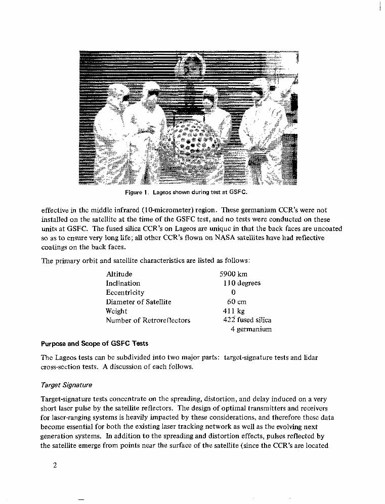
Figure 1 . Lageos shown during test a t GSFC.

effective in the middle infrared (1 O-micrometer) region. These germanium CCR’s were not installed on the satellite at the time of the GSFC test, and no tests were conducted on these units at GSFC. The fused silica CCR’s on Lageos are unique in that the back faces are uncoated so as to ensure very long life; all other CCR’s flown on NASA satellites have had reflective coatings on the back faces.

The primary orbit and satellite characteristics are listed as follows:

Altitude 5900 km Inclination 1 10 degrees Eccentricity 0 Diameter of Satellite 60 cm Weight 411 kg Number of Retroreflectors 422 fused silica

4 germanium

Purpose and Scope of GSFC Tests

The Lageos tests can be subdivided into two major parts: target-signature tests and lidar cross-section tests. A discussion of each follows.

Target Signature

Target-signature tests concentrate on the spreading, distortion, and delay induced on a very short laser pulse by the satellite reflectors. The design of optimal transmitters and receivers for laser-ranging systems is heavily impacted by these considerations, and therefore these data become essential for both the existing laser tracking network as well as the evolving next generation systems. In addition to the spreading and distortion effects, pulses reflected by the satellite emerge from points near the surface of the satellite (since the CCR’s are located

2

near the outer surface). However, in most geophysical applications, it is desirable to “correct” the range measurement so that it can be related to the center of gravity of the target, since it is this point whose motion through the Earth’s geopotential field can be precisely calculated. In general, this “correction” is a function of the attitude of the satellite with respect to the incident pulse. Because Lageos is a completely unstabilized target and because no information will be available on its attitude, it is important to: (1) measure the value of the range correction and (2) measure the amount of variation in this correction as a function of attitude. Attitude- dependent variations represent a noise source in the ranging system which may not be reducible through data averaging.

Lidar Cross Section

The lidar cross section (u) is the single parameter which quantifies the ability of a target to reflect incident energy in a specified direction (Reference 3). Because Lageos is in an orbit which is substantially higher than most of the other CCRequipped satellites (5900 km versus

, a typical 1000-km orbit), the radar link is much more difficult, making the absolute value of the lidar cross section extremely important. As discussed in Reference 3, a is a function of the characteristics of the incident signal (wavelength, polarization, and angle of incidence) and the direction of interest in the far field of the reflected signal. All these factors were modeled during the design phase of the Lageos CCR’s (Reference 4), but it was widely recognized that variations in the properties of individual cube corners due to material inhomogeneity and manufacturing tolerances could be substantial (Reference 5), and that the overall performance of an array consisting of several hundred of these reflectors could be significantly different than the computer model. With this motivation, extensive tests of the cross-section value and the far-field pattern of reflected signals from Lageos were carried out during this program.

TARGET SIGNATURE TESTS

The target signature tests were divided into three parts. The first part addresses the average spreading that is imposed on reflected laser pulses by the satellite reflectors. The second part consisted of measurements of the range corrections so that range measurements can be referenced to the satellite center of mass; the third part addresses the pulse-to-pulse waveform variations which result from coherent interference between the individual satellite reflectors. The tests are described in this order in the sections that follow.

Pulse Spreading

Physical Mechanism

The mechanism of pulse spreading can be understood by reference to figure 2. When a transmitted laser pulse illuminates the satellite, all the cube corners within approximately 525’ of the pulse propagation direction reflect significant energy back to the transmitter (Reference 5). Because these CCR’s are on the surface of a sphere, they are at different distances from the transmitter, and the pulses reflected back to the transmitter will be displaced in time (as

3

a. TRANSMITTED PULSE JL b. REFLECTED PULSES

SECTION OF SATELLITE REFLECTOR ARRAY

7 6 5 4 3 2 1

c. DETECTOR IMPULSE RESPONSE A d. DETECTOR OUTPUT

Figure 2. Array-induced pulse spreading.

shown in figure 2b). Generally, the receiver is collocated with the transmitter, and its output signal (figure 2d) is given by the convolution of its impulse response (figure 2c) with the received pulse train;* this pulse can be significantly broadened as compared with the return from a single CCR or a flat array of CCR’s aligned normal to the transmitted pulse (which would produce a detector output given by the convolution of figures 2a and 2c).

It should be noted that in those cases where the reflected pulses overlap in time (for example, pulses 5, 6, and 7 of figure 2), the resultant waveform is dependent on the relative phases of the optical fields of the respective pulses;? the impact of these coherent interactions on pulse spreading is discussed in the section, “Pulse Shape Variations due to Coherency Effects.” However, for average pulse-spreading considerations, these coherent effects can be neglected, and net reflected signal can be obtained by addition of pulse energies.

*In the more general case of separated transmitter and receiver stations, the effect is no different.

?In a rigorous sense, this is true only for the case of very high optical signal-to-noise (SNR) ratios. At low signal levels, the randomness induced by poissonian photoemission causes another degree of randomization of the output waveform (Reference 6) . The data to be reported here result from averaged waveforms built up using large numbers of optical pulses (typical lo4). hi^ averagingis equivalent to operating at very high SNR.

4

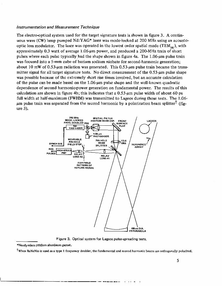
Instrumentation and Measurement Technique

The electroaptical system used for the target signature tests is shown in figure 3. A continuous wave (CW) lamp pumped Nd:YAG* laser was mode-locked at 200 MHz using an acousto- optic loss modulator. The laser was operated in the lowest order spatial mode (TEM,,), with approximately 0.3 watt of average 1.06-pm power, and produced a 200-MHz train of short pulses where each pulse typically.had the shape shown in figure 4a. The 1.06-pm pulse train was focused into a 5-mm cube of barium sodium niobate for second-harmonic generation; about 10 mW of 0.53-pm radiation was generated. This 0.53-pm pulse train became the transmitter signal for all target signature tests. No direct measurement of the 0.53-pm pulse shape was possible because of the extremely short rise times involved, but an accurate calculation of the pulse can be made based on the 1.06-pm pulse shape and the well-known quadratic dependence of second harmonic-power generation on fundamental power. The results of this calculation are shown in figure 4b; this indicates that a 0.53-pm pulse width of about 60 ps full width at half-maximum (FWHM) was transmitted to Lageos during those tests. The 1.06- pm pulse train was separated from the second harmonic by a polarization beam splitter (figure 3).

-t

200 MHz SPATIAL FILTER MODE-LOCKED ANDBCM BEAM EXP. FRONT

FREO. DOUBLED p

PATTERN OF FAR-FIELD

RETURN SIGNAL

Figure 3. Optical system for Lageos pulse-spreading tests.

*Neodymiunl yttrium aluminum garnet. tWhen BaNaNio is used as a type 1 frequency doubler, the fundamental and second harmonic beams are orthogonally polarized.

5

50 ps + c

X = 1.06 MICROMETERS FULL WIDTH AT HALF MAXIMUM: 90 ps

PULSE MEASURED BY GaAsSb PHOTODIODE

Figure 4a. Nd:YAG laser mode-locked pulse.

50 ps "t 4-

\ I X = 0.53 MICROMETERS FULL WIDTH AT HALF MAXIMUM: 60 ps

Figure 4b. Frequency doubled mode-locked pulse (calculated).

6

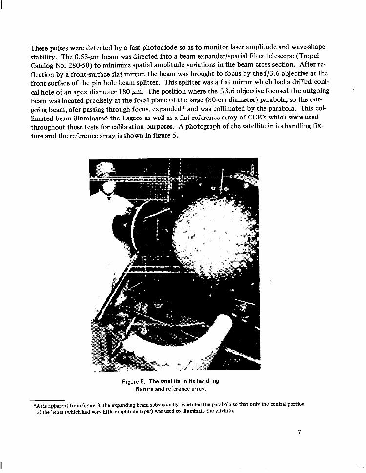
These pulses were detected by a fast photodiode so as to monitor laser amplitude and wave-shape stability. The 0.53-pm beam was directed into a beam expanderlspatial filter telescope (Trope1 Catalog No. 280-50) to minimize spatial amplitude variations in the beam cross section. After reflection by a front-surface flat mirror, the beam was brought to focus by the f/3.6 objective at the front surface of the pin hole beam splitter. This splitter was a flat mirror which had a drilled coni- cal hole of an apex diameter 180 pm. The position where the f/3.6 objective focused the outgoing beam was located precisely at the focal plane of the large (80-cm diameter) parabola, so the outgoing beam, afer passing through focus, expanded* and was collimated by the parabola. This collimated beam illuminated the Lageos as well as a flat reference array of CCR's which were used throughout these tests for calibration purposes. A photograph of the satellite in its handling fixture and the reference array is shown in figure 5.

Figure 5. The satellite in its handling fixture and reference array.

*As is apparent from figure 3, the expanding beam substantially overfilled the parabola so that only the central portion of the beam (which had very little amplitude taper) was used to illuminate the satellite.

7

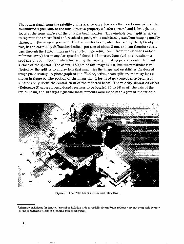
The return signal from the satellite and reference array traverses the exact same path as the transmitted signal (due to the retrodirective property of cube corners) and is brought to a focus at ~e front surface of the pin-hole beam splitter. This pin-hole beam splitter serves to separate the transmitted and received signals, while maintaining excellent imaging quality throughout the receiver system." The transmitter beam, when focused by the f/3.6 objective, has an essentially diffraction-limited spot size of about 3 pm, and can therefore easily pass through the 18.0-pm hole in the splitter. The return beam from the satellite (and/or reference array) has an angular spread of about f 45 microradians (pr), that results in a spot size of about 800 pm when focused by the large c,ollimating parabola onto the front surface of the splitter. The central 180 pm of this image is lost, but the remainder is reflected by the splitter to a relay lens that magnifies the image and establishes the desired image plane scaling. A photograph of the f/3.6 objective, beam splitter, and relay lens is shown in figure 6. The portion of the image that is lost is of no consequence because it subtends only about the central 20 pr of the reflected beam. The velocity aberration effect (Reference 3) causes ground-based receivers to be located 35 to 38 pr off the axis of the return beam, and all target signature measurements were made in this part of the far-field

Figure 6. The f/3.6 beam splitter and relay lens.

*Alternate techniques for transmitterieceiver isolation such as partially silvered beam splitters were not acceptable because of the depolarizing effects and multiple images generated.

8

pattern. Two types of field stops were used during these tests : (1 ) a small circular aperture of 0.1 8-mm diameter and (2) an annulus of 3-mm inner radius and 4-mm outer radius. With a receiver system focal length of 100 m, this corresponds to an angular subtense of 1.8 j.tr for the circular aperture and a transmission ring of 30 to 40 pr for the annulus. The energy passing through the field stop was collected by a relay lens and focused through an interference filter onto the photocathode of a high-speed photomultiplier (Varian Catalog No. 154). A photograph of the detector assembly is shown in figure 7. The manufacturer's performance specifications for this detector are given in the following list:

Designator Description

Photocathode/Window Material Cathode Diameter Cathode Quantum Efficiency Gain Number of Stages Dynode Material Anode Dark Current Output Current Bandwidth, 0 to -3 Decibel (db) Anode Rise Time (1 0% to 90%) Output Coupler Dimensions, Housed with Magnets Weight

S-20/Sapphire 5.08 mm (0.2 in) 10 Percent Typical at 5300 Angstrom (A) 1 O5 Typical 6 Becu Alloy 3 X 10'9Typical at 20°C 250-Microamps (PA) Maximum Continuous Direct Current (dc) to 2.5 Gigahertz (GHz) 150 Picoseconds (ps) 50-0hm Coaxial OSM 8.25 cm (3.25 in) X 6.68 cm (2.63 in) 15.87 cm (6.25 in) 1.81 kg (4 lb)

The photomultiplier output signal as well as a synchronized trigger signal from the laser were sent to the data system shown in figure 8. The sampled analog waveforms that were developed by the sampling system were digitized by a Tektronix R7912 and stored in the computer. The R79 12 supplied waveforms to the computer at a rate of approximately 10 per second. Typically, for a given set of test parameters, 100 waveforms were input to the computer, averaged by the computer, and the resultant waveform delivered to one of the output devices. Following the data taking, the averaged waveforms were recalled from storage and hardcopy generated. The waveforms were analyzed graphically to recover pulse shape characteristics and interpulse spacing. A photographic overview of the entire test area (with only the large collimator outside the frame) is shown in figure 9.

Results

The received waveforms that were analyzed during the target signature tests are shown schematically in figure 10. To make full use of the precision available from the time axis of the R79 12, the pulse pair shown in the figure was recorded for each of target signature tests. This reference-array pulse and the Lageos pulse differ only because of the planar and nonplanar characteristics of their respective cube corner arrays, and this fact was used to measure the pulse spreading induced on the laser pulse by the Lageos.

9

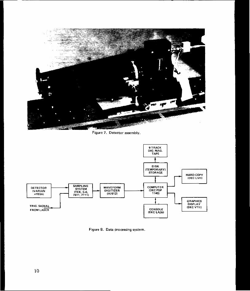
Figure 7. Detector assembly.

t DISK

(TEMWRARYI STORAGE

HARDCOPY (DEC LVII) t

t

P

DETECTOR - SAMPLING SYSTEM WAVEFORM

- COMPUTER (VARIAN

1140) (R79121 7Sl l . 7T l l l - n153Al

(DECPDP c DIGITIZER -c (TEK. s4, -

GRAPHICS

(DEC VTII) TRIG. SIGNAL FROM LASER

(DEC LA36) CONSOLE

- DISPLAY

Figure 8. Data processing system.

10

Figure 9. The test area.

RETURN SIGNAL

REFERENCE ARRAY

/- I"-. I

WAVEFORM ~--- \ - - - - - i / RECORDED \ r

LAGEOS

TIME *

Figure IO. Received waveform schematic.

11

The results of the pulse-spreading tests are shown in figure 1 1. The measured values vary from 21 0 ps to 260 ps depending on the orientation of Lageos with respect to the incident pulse. The satellite was rotated with respect to the incident pulse by the handling fixture shown in figure 5; however, the reference array was not changed and remained normal to the incident pulse throughout the tests.

PULSE WIDTH (FWHM) IN ps

+600- 230 230 240 230 240

+3W- 230 230 260 220 220 240 260 230 260

00 - 270 230 220 220 250 220 240 220 230 260 240 210 260 220

-300- 220 260 250 250 240 250 230 230 240 230

-600 - 250 240 240 230 260

AVERAGE VALUE 240 ps

00 300 600 900 1200 1500 180° 210° 2400 2700 3000 3300 3600

LAGEOS ORIENTATION (LONGITUDE)

I I I I I 1 I I I 1 1 I

0 WAVELENGTH 0.53 urn 0 ALL READINGS? 5 ps 0 INSTRUMENTATION SYSTEM RESPONSE

TIME (FWHM) 205 ps

Figure 11 . Pulse width of reflected signals from Lageos.

Because CCR's as much as 25' off-normal contribute to the return signal, a data point such as +60' latitude and 0" longitude, in fact, samples the satellite over the ranges of +35" to +85" latitude and 335" to 2.5' longitude. As shown in figure 1 1 , the average pulse width of the received signal was 240 ps. A sample of the measured waveforms is shown in figure 12.

The temporal resolution of the instrumentation system (as measured by the returned from the flat reference array) was 205 ps, so the instrumentation system (especially the photomultiplier) contributed significantly to the measured pulse width. The relative contributions of satellite and instrumentation system to the total pulse width can be evaluated to first order by assuming Gaussian waveshapes for both the reference array and Lageos signals. In this case, the pulse widths add in quadrature and the Lageos contribution can be easily evaluated. These results are listed in figure 13 and can be used to estimate the width of the reflected pulse from Lageos for arbitrary transmitter/receiver systems by carrying through the root-sum-squares (RSS) calculation.

12

K 0

i

. * .x L R F L O S T E S T D R T n = x * =

D R T E : 1 4 - J R N - 7 6 I r n r : II:BO:OB

s n T r L L I ? E L R T T : 0 D E G L O N G : 5 6 D E G L R S S R U R V E L E N G ? H : . 5 3 2 M l C X O N S

O F R V E R R G E D U ~ V E F O R M S : z o o 7 E L E M E N T S M O O T ~ I I N G

Figure 12. A sample of the measured waveforms.

-.

PULSE SPREADING (FWHM) IN ps

ffi00- 90 110 130 110 130

+300 - 60 120 160 80 90 120 150 120 160

00- 160 110 90 90 120 80 100 80 80 160 120

60 160 90 -300 - 40 160 140 160 120 130 100 120 120 90

-600 150 130 130 110 160

AVERAGE VALUE 120 ps I I I I I I I I I I I

00 300 600 900 1200 1500 1800 210° 2400 2700 30O0 3300 3600


0 WAVELENGTH 0.53pm 0 ALL READINGS f 5 ps

Figure 13. Pulse spreading induced by Lageos.

13

A motion picture camera was installed in the received optical system (figure 3) and relay lens-No. 1 was repositioned, so that an image of the rotating satellite (rather than the far- field pattern of the return beam) was recorded on film. Four of these frames are shown in figure 14. The brightness of the individual CCR is proportional to the total energy reflected by each. The arc of CCR’s in the lower right-hand corner is the reference array; each of the cubes in this array was normal to the incident beam, and therefore no brightness variation exists. Figure 14a shows a localized cluster of CCR’s dominating the return signal, and therefore very little pulse spreading would be expected at this satellite attitude. Figure 14b shows Lageos with its north pole aligned with the incident beam. The black spot in the center is the location of one of the germanium CCR’s. These CCR’s were not installed at the time of the tests, but even if they were in place, the results would not be different because germanium is opaque at visible wavelengths. Figure 14c shows the north pole again, but in an off- axis condition. Figure 14d is another orientation where significant pulse spreading can be expected. The amount of pulse spreading contributed by off-axis CCR’s can be estimated using the geometry of figure 15.* Inspection of these values and the frames of figure 14 show the reason for the pulse spreading variations listed in figure 11.

Analysis of the waveforms from the reference and satellite arrays shows that the Lageos- induced broadening is primarily an increase in pulse fall time, with pulse rise time changes too small to be measured. The data reported in this section were taken with a “point” aper-

a ture (0.9-pr radius) positioned 35-pr off-axis in the far-field pattern of the reflected beam. During an actual satellite pass, the ground-based receiver will change position in the far field, although always remaining 35- to 3 8 ~ offaxis. Accordingly, during these tests, data were taken with the “point” receiver at different locations in the 35- to 38-pr annular region. No significant difference from the data of figure 11 was noted. Data were also taken with the “point” aperture replaced by a 30- to 40-pr annular aperture. These data are effectively an average of the pulse shapes over the entire far-field region of interest. Again, no significant difference from the data of figure 11 was noted. In conclusion, the data of figure 11 are an accurate measure of the pulse-spreading characteristics of the Lageos, and this characteristic is not a sensitive function of receiver position in the far field.

Centerof-Gravity Correction

The range measurements from a ground station to Lageos during a typical satellite pass are, in fact, distance measurements from a well-defined point on the ground to a point approxi- mateIy 5 cm inside the surface of the Lageqs. The geophysical applications for which Lageos was launched require that the range measurements be “corrected” so that they can be interpreted as distance measurements to the center of mass of the satellite. To do this, it is necessary, to first define precisely the location of the equivalent reflection point within the satellite, and, secondly, to measure the variability of this point with satellite attitude, because this represents a potentially irreducible error source in the overall ranging system.

*An accurate calculation must take into account not only the energy reflected by each CCR but also the antenna pattern associated with each CCR return.

14

--___-..- ... . . .“ .“ ..._. - ~... ... - a .. 111 I I ....... I -.. .... 1

a .

C.

b.

d.

Figure 14. Lageos images for various orientations.

15

\ LAGEOS SURFACE - \

'\ ,A EFFECTIVE REFLECTION PLANE

' \ \ REFLECTED PULSE

TIME DELAY

104 ps

26 ps

0 PS PULSE

DIRECTION - LAG EOS

CENTER CCR

Figure 15. Effect of off-axis CCR's on pulse spreading.

Physical Mechanism

The equivalent reflection point for a solid cube corner is given by

where

AR is measured from the center of the front face of the cube comer to the reflection point

L is the vertex to front-face dimension

n is the refractive index of the material

8 is the angle of incidence

16

Using this equation and the geometry of figure 15 , it follows that the reflection planes for the first and second rows are 3.6 mm and 14.5 mm further into the satellite than that of the normal CCR. The total signal detected at the receiver station is the sum of the contributions from the individual CCR’s; therefore, with proper weighting, the received waveform could be calculated and the equivalent reflection plane, precisely defined. There are two difficulties which prevent this analytic treatment from being entirely adequate.

First, the proper weighting to apply to each of the CCR reflections is not known better than approximately k3 dB due to material and manufacturing variations inherent in high-gain CCR’s. Secondly, the geometry of figure 15 is merely one particular orientation of the satellite with respect to the incident pulse, and a shift of just 5’ of the (unstabilized) satellite would significantly change the relative positions of the individual CCR reflection planes. It is clear from the photographs of figure 14 that significant variations and asymmetries in the cluster of active Lageos CCR’s exist for different satellite attitudes.

The optical system that was used for the rangecorrection measurements and is shown in figure 16, was nearly the same as that used for the pulse-spreading tests (figure 3). The two differences are: (1) the insertion of a polarization rotator in the 0.53-pm beam just before the entry into the spatial filter-beam expander telescope assembly and (2) the insertion of a mask with a clear aperture equal to 1 cube corner diameter in front of the satellite. The data processing system was the same as described in the section, “Instrumentation and Mea- surement Technique” under “Pulse Spreading” and illustrated in figure 8.

Instrumentation and Measurement Technique

The measurement technique can be explained with the aid of figure 17. At the top of this figure, the Lageos is shown behind a mask which allows only the cube corner normal to the incident beam to be illuminated. This results in a signal So(t) at the output of the receiver, where R refers to the pulses from the flat reference array in front of the mask, and the Lageos single cube comer signal is as shown. The mechanical design of the Lageos places the front face of each of the CCR’s at a distance of 298.1 mm from the center of the satellite. There- fore, by using equation (2), the point within the satellite from which the single CCR pulse is reflected can be defined precisely in terms of its relation to the satellite center of mass; similarly, by measuring the A. value of So (t), the position of the reference array, with respect to the satellite center, can be defined precisely. Having recorded the So(t) signal, the mask was then removed, and the entire satellite was illuminated by the pulse train. This results in the signal S , (t) at the receiver output. The range correction, AR, for satellite orientation 1 can then be computed from

c*, AR, = 298.1 - (L) (n) - - (mm) 2

17

200 MHz SPATIAL FILTER

PATTERN OF RETURN SIGNAL

Figure 16. Optical system for Lageos range correction measurements.

where

L = 27.8mm

n = 1.455

t, = A, - A, (s)

This measurement sequence was repeated for a sufficient number of Lageos orientations so that the entire satellite was mapped. The numerical values for the range correction are slightly different depending on whether leading edge (half maximum) or peak detection is used in the receiver. Both sets of values were computed and are reported under “Results.”

Calibration

The instrumentation system used in these tests was evaluated in terms of its precision (or resolution) and absolute accuracy of time-interval measurement. The precision test consisted of illuminating the reference array and Lageos as in figure 17 (with mask removed), recording the received waveshape, measuring the time interval between the reference array and Lageos pulses, and repeating this measurement a number of times without any changes to the system.

18

MASK I

+I LAGEOS

REF. ARRAY

E I I I

INCIDENT PULSE I TRAIN I

I

RECEIVED SIGNAL

I / 1 \ PULSE F R O M SINGLE CCR

+"' * ATORIENTATION VJ, ,@, ) PULSE FROM ENTIRE SATELLITE

PULSE FROM ENTIRE SATELLITE AT ORIENTATION IO,. 0")

Figure 17. Measurement technique for Lageos.

The statistics of the time-interval measurement were computed, and the standard deviation of the measurement was defined as the system precision. One typical set of measurements is listed in table 1.

Precision checks were run several times during the course of the Lageos testing, and the results listed in table 1 are typical. To measure accuracy, the Lageos was removed from the collimated beam, and an additional flat array of CCR's was installed in front of (and to the side of) the reference array. The distance between the two arrays was measured with a caliper, and then the two arrays were illuminated by the laser pulses. The received pulses were recorded, and the time differential between the reflections from the two arrays was measured. This measurement of array spacing was then compared with the caliper measurement to evaluate absolute accuracy. The results of this test are listed as follows:

File No. Spacing (PSI

LR 581 1 1248 LR 5812 1250 LR 5813 1264 LR 5814 1248

19

I

File No. Spacing (ps)

LR 5815 1262 LR 5816 1247 LR 5819 1243 LR 5820 1252

Predicted Pulse Spacing (Based on Caliper Measurement) = 1255 ps Average Difference (Measured-Predicted) = 3 ps (0.5 mm)

File No.

LR 1429 LR 1430 LR 1431 LR 1432 LR 1434 LR 1435 LR 1436 LR 1438 LR 1439

Table 1 Instrumentation System Precision

Time Interval (ps) (Half Max. to Half Max.)

140 143 143 152 143 143

1137 1143 1134

~~ ~~

Time Interval (ps) (Peak to Peak)

1131 1120 1117 1137 1114 1120 1137 1134 1131

~

Standard Deviation (Half Maximum) = 3.8 ps (0.6 mm) Standard Deviation (Peak) = 8.9 ps (1.3 mm)

Based on these precision and accuracy tests, it is estimated that the pulse measurements are correct to within +1 mm (or +7 ps).

Results

The range correction measurements for Lageos using the criterion of leading edge/half-maximum detection are given in figure 18. The average value is 25 1 mm with a variability of standard deviation 1.3 mm. The data points at locations -27' latitude and 7" longitude and -27" latitude and 123' longitude and at the north pole correspond to germanium CCR positions. Some re- duction in range correction at these locations is apparent as would be expected.

A similar range-dorrection map is shown in figure 19 for the case of peak detection at the receiver. The average correction is slightly less at 249 mm and has a variability with a standard

20

+700 LAT.

DEVIATIONS FROM MEAN IN MM (MEAN VALUE = 251 MM)

K 0

+600

+30°

00

-300

-60'

- -1 2 1 1 0

- -1 1 0 0 1 -1 0 -1 1

"I 0 -2 -1 -3 -1 -1 1 0 1 3

- -10 0 -3

2 1 2 -1 1 0 2 0

- 0 1 2 0 1

I ' I 1 1 I 1 I I I I I 00 300 600 900 1200 1500 180° 210° 240° 2700 3000 330° 3600


-700 LAT.

WAVELENGTH: 0.53 RECEIVER FIELD OF

Clm VIEW: 1.8 Br DIA.

Figure 18. Lageos range-correction map-half-maximum detection.

21

+700 LAT

DEVIATIONS FROM MEAN IN MM (MEAN VALUE = 249 MM)

- w n 3 6 0 0 - k

-3 -1 -1 2 -2

l-

0 -1 2 0 0 0 0 -2 1 d +300 - a z 0 2 00"l

0 -1 2 o - ~ 2 0 0 0 3 1 PC -300 - -1 5 0 -3 0 -4 +1 0 1 1 0 2

I-

0 0 v)

-600- 0 3 3 -2 0

4 .. ~. -

3 1 -

I 1 00 300 600 900 120° 1500 180° 2100 2400 270° 30O0 3300 3600


-70' LAT WAVELENGTH: 0.53 RECEIVER FIELD OF

P m VIEW: 1.8 p r

Figure 19. Lageos range-correction map-peak detection.

22

deviation of 1.7 mm. The range-correction variations for both the half-maximum and peak detection cases are significantly less than the 5-mm systems specification.

The data of figures 18 and 19 were taken with a 1.8-pr receiver field stoppositioned 35 pr off the center line of the return beam. Additional measurements were taken to determine if the location of the receiver in the far-field pattern would have any effect on the range correction.* The receiver was positioned at four different locations (separated by 90”) in the far field and reference array/Lageos pulse spacing measured. No significant variations were found; peak deviations in the range correction were approximately 2 mm.

Range-correction measurements were also taken with the annular-field stop in the receiver system; this essentially averages out any positiondependent variations which do exist. These results are shown in figure 20, where the listing at the top refers to leading edge half-maximum detection and the values at the bottom are for peak detection. As expected, the variations are somewhat less, with the half-maximum values having a standard deviation of 0.2 mm and the peak detection values having a standard deviation of 1.3 mm..

The effects of transmitter polarization on range correction were also investigated. The satellite was illuminated with a circularly polarized beam, as well as three different linear polarizations; the range correction was measured for each case. No statistically significant differences were ob served.

Pulse Shape Variations Due to Coherency Effects

As noted in the section, “Physical Mechanism” under “Pulse Spreading” and figure 2, the laser pulses returned by the individual retroreflectors on the satellite often overlap in time, and therefore the net field strength at the photodetector is determined by the coherent addition of the fields from the individual pulses. These optical fields have phases that are not predictable, and therefore the detected pulse shape can be expected to show some amount of randomness. Since the time-of-flight measurement is referenced to some point on the return signal waveform, this variation in received wave shape will introduce some amount of error in the range measurement.

No direct measurements of single-shot Lageos reflected signals which had sufficient bandwidth to show coherent fading were made during this test program. The technology to perform such measurements is available) but is very complex and could not be fitted into the very tight prelaunch schedule.

However, computer calculations were carried out which provide a good estimate of the magnitude of this effect. The program for these calculations (Retro-Lageos) was developed by one of the authors (P. 0. Minott) and can be used for cube corner arrays of arbitrary geometry.

*This is important because in typical ground stationarbiting satellite geometries, the receiver position in the far field of the return beam moves nearly 180” around the annulus from beginning to end of a pass.

tStreak tubes have sufficient bandwidth and sensitivity to make single shot measurements.

23

DEVIATIONS FROM MEAN IN MM - HALF MAX. DETECTION

-1 1

0 0 -1

- 1 0 0 0 0 0 0 - 1 0

0 1 -1 0 0 -1 0 1 -1 0

1-1 1 2 1 - 1 1 0 0 1 " 0 0 0

1 1 1 0

DEVIATIONS FROM MEAN IN MM - PEAK DETECTION

1

t I I I I I 1 I I I I 1 00 300 600 90° 120° 150° 1800 210° 2400 270° 3W0 3300


WAVELENGTH: 0.53 .urn RECEIVER FIELD OF VIEW: 30 - 40 P r ANNULUS

Figure 20. Range-correction measurements taken with annular-field stop in receiver system.

24

The calculation procedure for Lageos was as follows:

1. The satellite orientation with respect to the incident pulse was specified. In this case, the face of the south-pole cube corner was normal. to the incident beam..

2. The satellite was illuminated with a plane wave of specified wavelength, polarization, and shape; in this case wavelength was 0.53 pm, polarization was vertical, and pulse shape was Gaussian with a 63-ps standard deviation.

3. Each of the participating retroreflectors reflects back a signal whose magnitude is proportional to the lidar cross section of the retroreflector and whose phase depends upon its position.

4. To determine the magnitude of the pulse from each retroreflector, the program cal- culates a far-field-diffraction pattern (FFDP), computes the position of the receiver (including velocity aberration effects), and assigns the value corresponding to this point as the energy of the reflected pulse.

5. Each cube comer produces a pulse with identical temporal width but with differing peak positions due to the different distances of the individual retroreflectors from the laser source. The program accounts for this by calculating the optical line-of-sight distance from the reflection point of each cube corner to the satellite center of gravity (CG). This is converted to a temporal delay of each cube corner pulse referenced to the spacecraft CG.

6. When the pulses returned from each cube corner are known, both from a magnitude and temporal delay standpoint, the pulses are summed to obtain the net array pulse. However, a simple summing of the wave forms from all the retroreflectors would produce only the incoherent wave shape. Therefore, the square root of each pulse magnitude is taken to convert to a term proportional to the optical field strength, and a random number generator is used to assign phases between 0 and 2a radians. The resultant pulses are then summed to obtain the coherent field strength pulse shape of the array. To convert back to signal strength, the resultant pulse magnitude is then squared.

7. At this point, a single coherent pulse shape has been generated. To determine the statistics of the pulse centroid position, the process is repeated several hundred times , and a histogram of the pulse centroid position is developed.

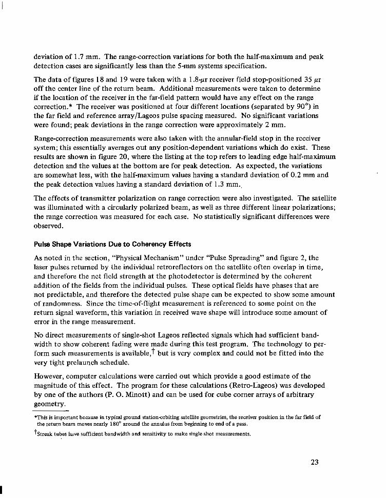
Figure 2 1 gives the results of these calculations for Lageos. Even with all other system parameters fixed, it is apparent that the centroid of the reflected pulse can undergo peak-to-peak excursions of several hundred ps. The standard deviation of the received pulse is calculated to be 77 ps. Taking into account that each measurement is a two-way (or double pass) range measurement, this standard deviation becomes 1.15 cm in range.

Clearly, an error source of this magnitude is very significant for Lageos tracking. However, the pulse shape variations that cause this should be essentially uncorrelated over time'intervals of

25

CENTROIDS (COMPUTER CALCULATION) HISTOGRAM OF REFLECTED PULSE

c

RELATIVE PROBABILITY r DEVIATION = 77 PS

STANDARD

1 3 1 c I

-800 -600 -400 -200 0 200

TIME DEVIATION (PSI

Figure 21. Lageos pulse shape variations due to coherent fading.

approximately 1 second (which is the typical spacing of range measurements), and therefore data averaging over measurement sets of 10 would effectively reduce this error source to approximately 4 mm.

LIDAR CROSSSECTION TESTS

Introduction

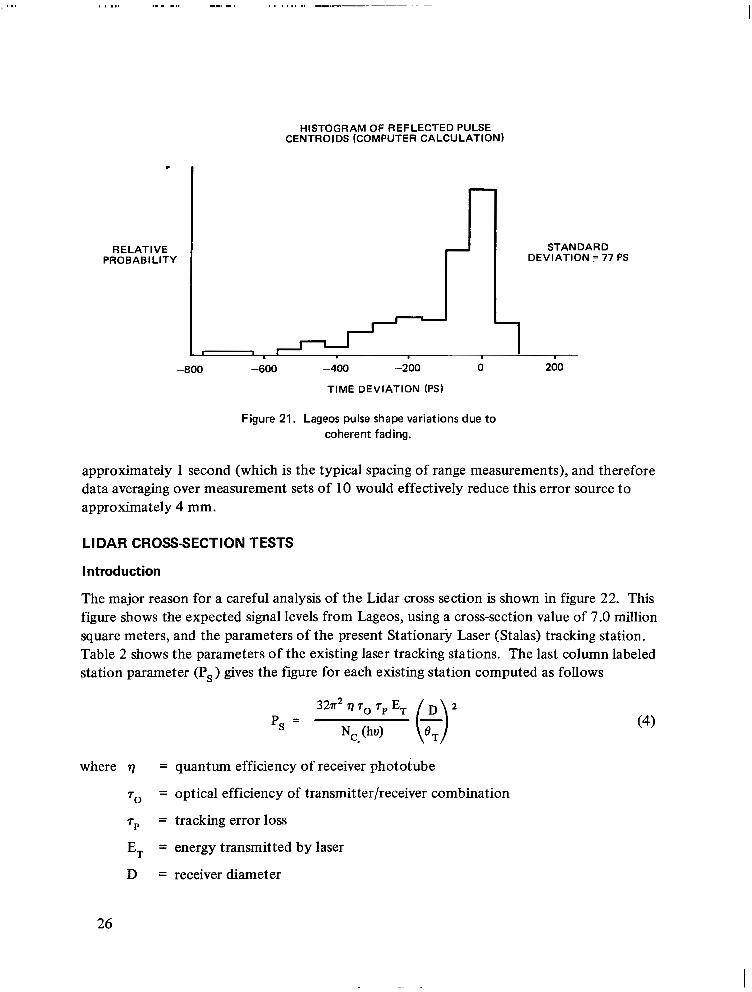
The major reason for a careful analysis of the Lidar cross section is shown in figure 22. This figure shows the expected signal levels from Lageos, using a cross-section value of 7.0 million square meters, and the parameters of the present Stationary Laser (Stalas) tracking station. Table 2 shows the parameters of the existing laser tracking stations. The last column labeled station parameter (P,) gives the figure for each existing station computed as follows

32a2 77 r r E P, = O (:)2

N q (hu)

where r ) = quantum efficiency of receiver phototube

T~ = optical efficiency of transmitter/receiver combination

T~ = tracking error loss

E, = energy transmitted by laser

D = receiver diameter

26

N, = number of photoelectrons required for an acceptable range measurement

hu = energy of a photon at the laser wavelength

8, = transmitter divergence to the 1 /e2 intensity points (Gaussian profile assumed)

In this table, N, has been set at 1.

w I: a a UI n.

200

180

160

140

120

1 0 0

80

60

40

20

0

LAGEOS SIGNAL STRENGTHS

I - "7 I I I

LIDAR CROSS SECTION

7 MILLION SQUARE METERS

- __"""" -""" "~"~-,""--"- - I ". 1

0 10 20 30 40 50 60 70 80 90

ZENITH ANGLE-DEGREES

Figure 22. Lidar cross-section analysis.

From figure 22, it can be seen that at 70" zenith angle only 9 photoelectrons are received, while at 50" zenith angle only 50 photoelectrons are received. Figure 23 shows the root- mean-square range error to be expected for various signal levels. Clearly, the accuracy of Lageos ranging is severely limited at present and for the near future by the small cross section of the satellite. However, because Lageos is expected to have a useful lifetime of several decades, improvements in ground-station technology should reduce this problem. As shown in figure 23, an increase of 10 to 20 times in ground-station effectiveness will be required to fully utilize the accuracy inherent in the Lageos array.

Because of the very weak signal levels, it was decided that a careful analysis of the Lidar cross section was necessary. The results of this analysis shown in the following sections indicate that while the average cross section is approximately 70 percent of its design value (1 0 million

27

Table 2 Parameters of Existing and Proposed

Laser Tracking Stations

Tracking I I E, Station (joules)

SA0 1 SA0 2 SA0 3 MOBLAS 2 MOBLAS 1 MOBLAS 3 MOBLAS 4" MOBLAS 5"

' MOBLAS 6" MOBLAS 7" MOBLAS 8" STALAS

6943 6943 6943 6943 6943 6943 5320 5320 5320 5320 5320 5320

0.50 0.50 0.50 0.25 0.80 0.80 0.25 0.25 0.25 0.25 0.25 0.25

*Under development

2 0 t " 1 1 A

w

0 1 0 20 30 ~0 sa ma 70 130 90 10~3 PHRTDELECTRRN5

Figure 23. Range error versus signals.

28

square meters (m2)), for certain conditions it drops by nearly an order of magnitude. The effects noted are expected to result in considerable changes in the method of operation of the ground tracking networks.

Instrumentation

Description of Test Equipment

In the following paragraphs, the design parameters of the test equipment used for the Lageos FFDP tests are discussed.

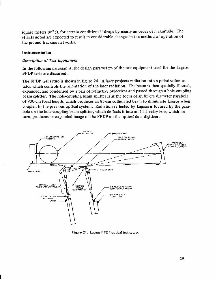
The FFDP test setup is shown in figure 24. A laser projects radiation into a polarization rotator which controls the orientation of the laser radiation. The beam is then spatially filtered, expanded, and condensed by a pair of refractive objectives and passed through a hole-coupling beam splitter. The hole-coupling beam splitter is at the focus of an 85-cm diameter parabola of 900-cm focal length, which produces an 85cm collimated beam to illuminate Lageos when coupled to the previous optical system. Radiation reflected by Lageos is focused by the parabola on the hole-coupling beam splitter, which deflects it into an 1 1 : 1 relay lens, which, in turn, produces an expanded image of the FFDP on the optical data digitizer.

-SATELLITE LAGEOS

7 IMAGING LENS

V

Figure 24. Lageos FFDP optical test setup.

29

. . .,

Several lasers were used in the FFDP tests to evaluate the performance of Lageos at different wavelengths. The parameters of these lasers are shown in table 3.

Characteristic T Wavelength (pm) Average Output (0) Transverse Mode Structure Amplitude Stability Polarization Polarization Purity

Table 3 Laser Parameters

HeCd

0.44 1 € 0.0 17

+5% Linear 1000: 1

-

TEMOO

~~

Laser Type

HeNe

0.6328 0.0 10

+3% Linear > 100: 1

TEMOO

~~~ ~~

- ~

Nd:YAG

1.064 0.350

+5% Linear > 50:l

TEMOO

~~

0.532 0.0 10

+lo% Linear > 50: 1

TEMOO

The polarization rotator consists of a Gaertner Babinet-Soled compensator, which acts as a X/4 plate to produce circularly polarized radiation. This is followed by a Nichol prism, which selects the desired polarization when a plane polarized beam is desired. The Nichol prism is removed from the system on all tests denoted as circularly polarized. The adjustable nature of the Babinet-Soleil compensator allows it to be adjusted to h/4 for any desired wavelength. Tests confirmed a better than 100: 1 extinction ratio for the cross polarization when in the plane-polarized mode.

A Spectra Physics Model 33 1 /332 beam expander/spatial filter was used to expand the laser beams to 50 mm and to spatially filter the laser beams. This was followed by a second Model 33 1 collimating objective, which focuses the beam on a holecoupling beam splitter.

The hole-coupling beam splitter consists of a 25.4-mm (1-in.) diameter, 2.99-mm (0.1 18-in.) thick fused silica flat inclined at 45" to the axis of the transmitted beam. At the center of this flat, a cone-shaped hole (f/3.0) is drilled from the back, through the flat, along the axis *

of the transmitted beam. The hole in the front reflective face of the flat is a 45" ellipse with a 1 8 0 - p minor diameter. The reflective face is flat to a tolerance of 1 /4 wave and aluminized and overcoated with SiO. Because this flat is the only polarization sensitive element in the system, its reflectivity was checked as a function of polarization orientation and was found to be constant within 5 percent.

The parabola is a 900-cm focal length, 85-cm aperture aluminized fused silica element. Its full aperture resolution is on the order of 50 pry but it is diffraction-limited over any 3.81- cm element. The source (located at the hole-coupling beam splitter) was placed in the focal plane, but off-axis in the horizontal direction by 35 cm. The parabola was, therefore, working in a 2.23" off-axis condition.

30

The satellite (Lageos) is supported in a fixture that allows it to rotate about the polar or equatorial axes built into the Lageos structure. The rotation axes can also be tilted relative to the optical axis and in a vertical plane by +goo. This allows the satellite to be viewed from any combination of latitude and longitude. (See figure 5.)

The 60-cm reference flat shown in figure 24 is accurately aligned normal to the incident radiation, and is used for calibration of the spatial scale of the FFDP and its intensity calibration. The flat is aluminized and overcoated with Si0 and has a reflectivity of 92 percent at 6328 A. Its use is further described in a future section of this document.

The reflected FFDP from Lageos was imaged on the hole-coupling beam splitter by the 900-cm parabola. Because this scale was incompatible with the optical data digitizer, an 1 1 : 1 relay lens was used to lengthen the effective focal length to 100 meters.

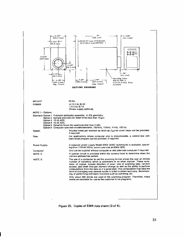
The optical data digitizer (ODD) is basically a computer-controlled digital video camera that can be commanded by a computer to scan the image and store the intensity values for each coordinate location in digital form. Its characteristics are shown in figure 25. The ODD was controlled by a PDP-11/40 computer and was modified by incorporating an electromechanical shutter that could be computer controlled. Exposures were made at 2.5 ms to eliminate image motion. A narrow-band interference filter was used to eliminate stray room light, and neutral density filters were used for additional control over exposure.

Spatial Resolution

The goal of the optical systems used for the Lageos FFDP tests was to obtain a spatial resolution of 5 pr. The primary source of aberration was the 85cm parabola used to collimate the radiation incident on the spacecraft. Because it was necessary to produce an obscuration- free beam, the parabola could not be used onaxis. It was therefore used 2.23O off-axis, which allowed the source to be 35-cm off-axis and prevented the source from obscuring the satellite. It is well known that the aberrations of a parabola off-axis are quite severe, and if it had been necessary to use the entire beam, the aberrations would have been intolerable. However, the retroreflective nature of the cube corners compensates for all aberrations of the collimator except those occurring within the aperture illuminating an individual cube comer. Therefore, the collimator effectively had an aperture of 3.81 cm, and with a focal length of 900 cm was working at f/236. In order to determine the image quality, a ray trace was done using the GOALS Program, which resulted in the data shown in figure 26. The geometrical ray tracebay distribution in the system focal plane for perfect retroreflector is listed as fo~~ows:

Percent Diameter Total Rays Microradians (Fr)

10 20 30 40 50

1.2 2.0 2.4 3.4 4.6

31

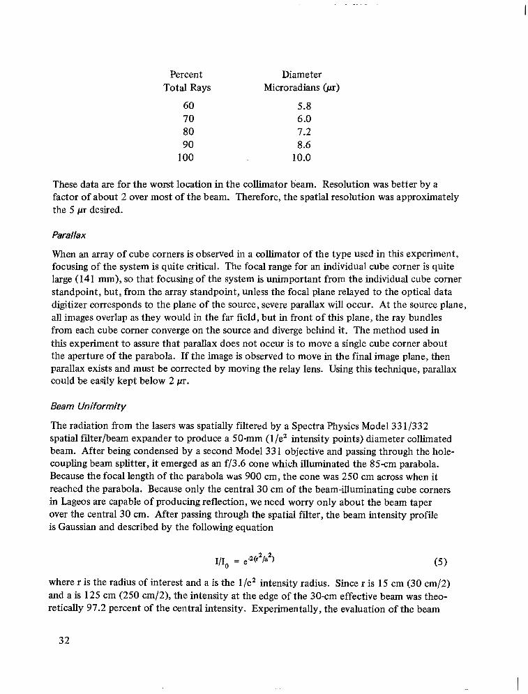
Percent Diameter Total Rays Microradians (pr)

60 70 80 90

100

5.8 6 .O 7.2 8.6

10.0

These data are for the worst location in the collimator heam. Resolution was better by a factor of about 2 over most of the beam. Therefore, the spatial resolution was approximately the 5 pr desired.

Parallax

When an array of cube corners is observed in a collimator of the type used in this experiment, focusing of the system is quite critical. The focal range for an individual cube corner is quite large (141 mm), so that focusing of the system is unimportant from the individual cube corner standpoint, but, from the array standpoint, unless the focal plane relayed to the optical data digitizer corresponds to the plane of the source, severe parallax will occur. At the source plane, all images overlap as they would in the far field, but in front of this plane, the ray bundles from each cube comer converge on the source and diverge behind it. The method used in this experiment to assure that parallax does not occur is to move a single cube corner about the aperture of the parabola. If the image is observed to move in the final image plane, then parallax exists and must be corrected by moving the relay lens. Using this technique, parallax could be easily kept below 2 pr.

Beam Uniformity

The radiation from the lasers was spatially filtered by a Spectra Physics Model 33 1 /332 spatial filter/beam expander to produce a 50-mm (1 /e2 intensity points) diameter collimated beam. After being condensed by a second Model 33 1 objective and passing through the hole- coupling beam splitter, it emerged as an f/3.6 cone which illuminated the 85cm parabola. Because the focal length of the parabola was 900 cm, the cone was 250 cm across when it reached the parabola. Because only the central 30 cm of the beam-illuminating cube corners in Lageos are capable of producing reflection, we need worry only about the beam taper over the central 30 cm. After passing through the spatial filter, the beam intensity profile is Gaussian and described by the following equation

where r is the radius of interest and a is the 1 /e2 intensity radius. Since r is 15 cm (30 cm/2) and a is 125 cm (250 cm/2), the intensity at the edge of the 30cm effective beam was theo- retically 97.2 percent of the central intensity. Experimentally, the evaluation of the beam

32

EMR 1 EMR PHOTOELECTRIC

GENERAL

computer could synthesize i t into meaningful information. The new E M R Optical Data Digitizer has Until quite recently, visucl data had to be manually or mechanically pre-processed before the

made this off-line pre-processing a thing of the past. With the O.D.D. the computer perceives visual data on-line as it determines what should be looked at and for how long.

O.D.D. expands the service capability of the computer into visual applications whose scope i s limited By eliminating the pre-processing operation and by permitting the selection of pertinent input, the

only by the imagination of the user and his software capabilities.

HOW THE O.D.D. WORKS The Optical Data Digitizer creates the binary equivalent of a two-dimensional optical image and thus prepares i t for. immediate input for the computer. Having complete control over the O.D.D. scan along the X, Y coordinates enables the computer to select the size of each scanning step, choose the direction of the scan, determine the dwell time per element, all with random access capabilities. The computer based on predetermined instructions, can then perform computations and initiate pro- cedures in accordance with the kind of dato it receives. It can also perform arithmetic functions such as summing, averaging over several cycles, deconvolving, or formatting for tape entry.

To accommodate the wide range of applications for which the O.D.D. can be utilized, a choice of image sensors i s available and includes the highly reliable E M R Image Dissector and a number of vidicon sensors (SEC, SIT/EBS, Sb,S,, PbO, or Si).

The mode of converting the optical image into its electronic equivalent varies with the sensor. Using the Image Dissector, conversion takes place by scanning an electronic image emitted by a target across an aperture. Vidicon sensors, on the other hand, perform this function by holding the corresponding charge pattern on a target for subsequent read-out by one electron beam. The deflection field for either type of sensor i s provided by a scanning-function driver which receives its analog voltage input from a scanning-function decoder. This permits the digital output of the computer to be used in controlling the scanning pattern within the sensor.

In the case of vidicon sensors, the electron charge-level output of the sensor i s translated by the intensity-function detector into voltage or current levels suitable for input to the intensity-function encoder far A/D conversion. The resultant binary signal i s stored and processed by the computer, which then prints out, displays, or formats for tape entry any pertinent information about the data determined by the software program.

Figure 25. Copies of EMR data sheets (1 of 4).

33

Model 658 A

ELECTRO-OPTICAL Sensor: Optics: Input Window: Input Image Size: Recommended Sensor Illumination Range: Signal Transfer Function: Uniformity: Elemental Exposure Time: Sensor Modulation Transfer Function:

Maximum Readout Time: Photocathode Dark Current:

ADDRESS & DATA Commandable Data Points:

Addressing Accuracy: Addressing Time: Speed:

Signal-to-noise Ratio:

Encoder:

ENVIRONMENTAL Operating Temperatures: Operating Humidity: Vibration:

Shock:

Storage Temperature:

COMPUTER RELATED

Interface:

Software Provided: Peripherals:

SPURIOUS EMISSION:

EMR Model 575 Image Dissector. Specified or provided by customer. 7056 Glass flat, .080"( 2.03mm) thick or fiber optic. 28 mm x 28 mm or any format less than 43 mm diagonal.

Five to 50 foot-candles. Unit gamma throughout range. f20% absolute, will not change faster than 2%/mm Controlled in software.

:G!G } with 19 Micron aperture.

Controlled in software. 1oJ electrons/sec/cmz. nominal at 20°C

4096Xlocations x 4096Y locations max. .03% RMS data point repeatability. Randomly addressable. Error at any point in field: 3% of field (referred to optical input). 5% optional.

Depending upon address, 2ps for 1% of field, 30ps for full axis. Processing time per element is controlled in software. For small steps, 50ps per element is typical. Dependent upon number of quantum events per exposure time. Given by: SIN = 1 . 2 2 d F d = aperture dia. In mils E = face plate illumination in foot candles At = dwell time.ps 8 bit ADC standard, 4 p s conversion time. 10 B 12 bit optional, also 4 ps conversion time.

Specifications valid at ambient temperatures from 60-90°F (16-32°C). Less than 80% R.H. MIL-STD-81OB. Method 514, Procedure X "Shipment by Common Carrier" (5G) MIL-STDdlOB, Method 516. Procedure V "Bench Handling" and Procedure VI "Rail Impact Test." 32-131°F (0-55°C).

All interfacing is accomplished via the computer. No direct interface with the camera is required. Test connectors are provided for real time monitoring at the camera head. Camera control and camera scanning. Computer equipment may be interfaced normally. The camera interface card requires one slot.

FCC Ruling (Part 15) "Unintended Radiation."

~


34

~ 15" (381 mm) -1 i ( 3 3 . 3 mm)

1 5/16''

29/32 ( 2 3 mm) STANDARD 3 1 / 3 2 (24.6 m r n ) O P T I O N I

OUTLINE DRAWING

WEIGHT 20 Ibs. POWER f 1 5 V d c @ 2 A

+ 5 V d c @ l A (Power supply optional)

NOTE 1 -Options: Standard:Option 1 Precision deflection assembly, f . 5 % geometry.

Option 2 Sample and hold (for dwell times less than lops ) . Option 3 10 bit ADC. Option 4 12 bit ADC. Option 5 Dynamic focus (for apertures less than 2 mil). Option 6 Computer selected variable bandwith, 100 kHz. 10'kHz. 1 kHz. 100 Hz.

Speed:

Size:

Process times per element as short as 2 p s for small steps can be provided. if required. For applications where computer size is objectionable, a control box with hard wired program can be provided, If required.

Power Supply:

Computer: NOTE 2:

NOTE 3:

A separate power supply Model 635A (635C rackmount) is available. operating from 1 l5VAC 6OHz. same case size as 658A ODD. Unit can be supplied without computer or with alternate computer if required. A special circuit is provided within the camera head to determine when the camera address has settled. The use of a computer to set the scanning format allows the user an infinite number of variations which is obtainable in no other manner. These Varia- tions, of course, include direction of scan, size of scanning step. random access, and dwell time per element change as well as the ability to perform computations from the data as it is generated. This computation may take the form of averaging over several cycles in order to obtain accuracy, deconvolving. or performing arithmetic functions such as summing, etC. Only about 200 words are used in the scanning program. Therefore, many words are available for use by the customer in his programs.


35

- (x,Y) FROM BINARY

COMPUTER

Basic ODD Block Diagram

. .. .


36

0 2 4 6 8 10

IMAGE DIAMETER (MICRORADIANS)

Figure 26. Geometrical ray tracehay distribution in system focal plane for perfect retroreflector.

uniformity indicated no areas within the 85-cm aperture, which were less than 92 percent of the peak value.

Parameters

The FFDP of the Lageos is a function of wavelength, state of polarization, and aspect angle of the satellite. Therefore measurements were made at several wavelengths (4416 a, 5320 A, 6328 A, and 10,640 A) arid several states of polarization (vertical, 45", horizontal, and circular) to investigate the behavior of the satellite for these various conditions. Due to the symmetrical nature of the satellite, only slight changes in its FFDP with aspect angle were expected or noted. Therefore, an average FFDP was obtained for each wavelength and state of polarization by taking a FFDP at each of the 55 locations shown in the following list:

Latitude (Degrees) Longitude (Degrees)

90 0 70 0,60, 120, 180,240,300 60 0,60, 120, 180,240,300 30 0,30,60,90, 120, 150, 180,210,240,270,300,330 0 0,30,60,90,

30 0,30,60,90, 120, 150, 120, 150,

180,210,240,270,300,330 180,210,240,270,300,330

37

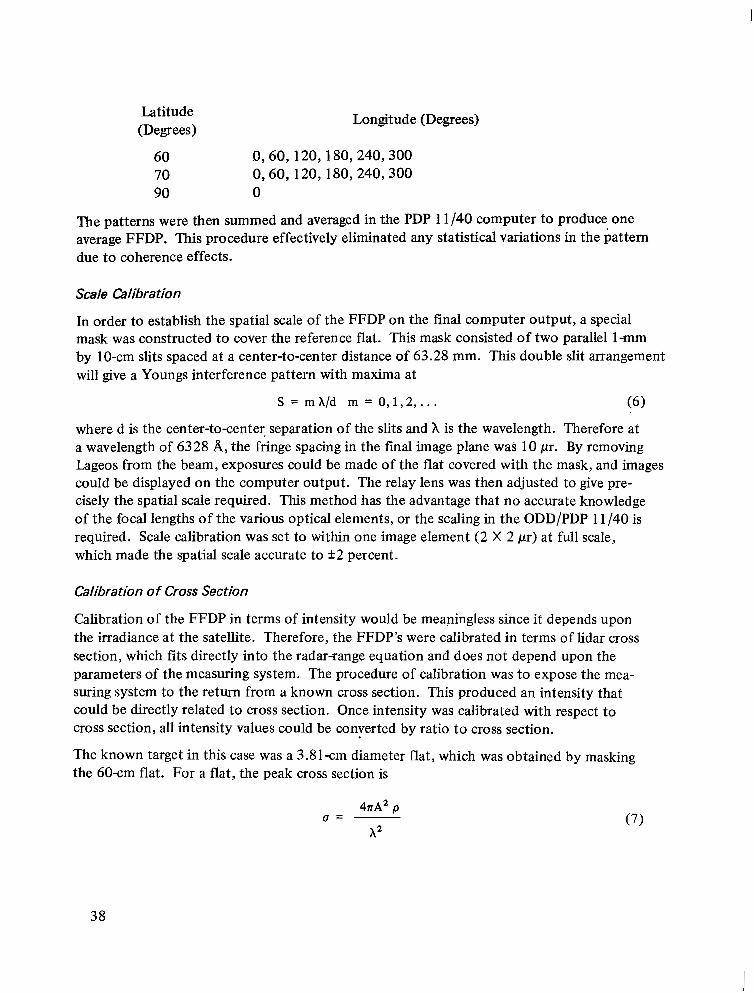
Latitude (Degrees)

Longitude (Degrees)

60 0,60,120,180,240,300 70 0,60, 120, 180,240,300 90 0

The patterns were then summed and averaged in the PDP 1 1/40 computer to produce one average FFDP. This procedure effectively eliminated any statistical variations in the pattern due to coherence effects.

Scale Glibration

In order to establish the spatial scale of the FFDP on the final computer output, a special mask was constructed to cover the reference flat. This mask consisted of two parallel 1-mm by IO-cm slits spaced at a center-to-center distance of 63.28 mm. This double slit arrangement will give a Youngs interference pattern with maxima at

S = mX/d m = 0 ,1 ,2 , ... (6)

where d is the center-tocenter. separation of the slits and X is the wavelength. Therefore at a wavelength of 6328 A, the fringe spacing in the final image plane was 10 pr. By removing Lageos from the beam, exposures could be made of the flat covered with the mask, and images could be displayed on the computer output. The relay lens was then adjusted to give precisely the spatial scale required. This method has the advantage that no accurate knowledge of the focal lengths of the various optical elements, or the scaling in the ODD/PDP 1 1 /40 is required. Scale calibration was set to within one image element (2 X 2 pr) at full scale, which made the spatial scale accurate to +2 percent.

Calibration of Cross Section

Calibration of the FFDP in terms of intensity would be meaningless since it depends upon the irradiance at the satellite. Therefore, the FFDP’s were calibrated in terms of lidar cross section, which fits directly into the radar-range equation and does not depend upon the parameters of the measuring system. The procedure of calibration was to expose the measuring system to the return from a known cross section. This produced an intensity that could be directly related to cross section. Once intensity was calibrated with respect to cross section, all intensity values could be converted by ratio to cross section.

The known target in this case was a 3.81cm diameter flat, which was obtained by masking the 60cm flat. For a flat, the peak cross section is

4nA2 p ( J = - A2

38

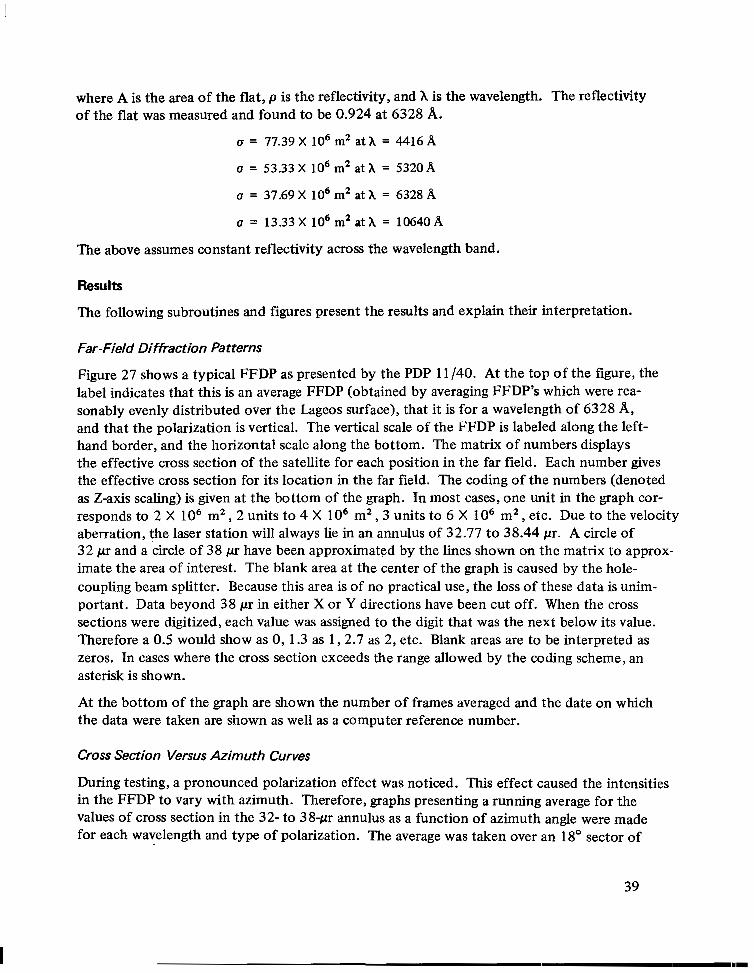
where A is the area of the flat, p is the reflectivity, and X is the wavelength. The reflectivity of the flat was measured and found to be 0.924 at 6328 A.

u = 77.39 X lo6 m2 at X = 4416 A

u = 53.33 X lo6 m2 at X = 5320

u = 37.69 X lo6 m2 at X = 6328 A

u = 13.33 X lo6 m2 at X = 10640 A

The above assumes constant reflectivity across the wavelength band.

Results

The following subroutines and figures present the results and explain their interpretation.

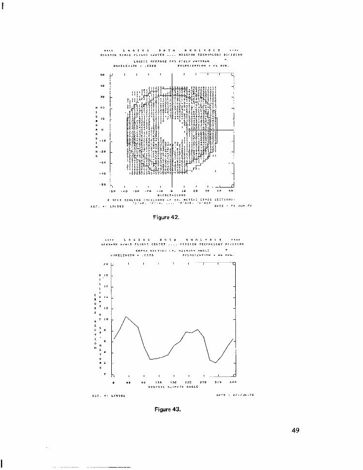
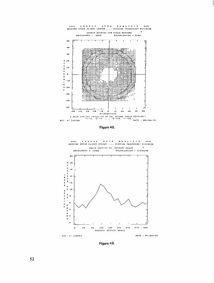
Far-Field Diffraction Patterns

Figure 27 shows a typical FFDP as presented by the PDP 11 /40. At the top of the figure, the label indicates that this is an average FFDP (obtained by averaging FFDP's which were rea- sonably evenly distributed over the Lageos surface), that it is for a wavelength of 6328 A, and that the polarization is vertical. The vertical scale of the FFDP is labeled along the left- hand border, and the horizontal scale along the bottom. The matrix of numbers displays the effective cross section of the satellite for each position in the far field. Each number gives the effective cross section for its location in the far field. The coding of the numbers (denoted as Z-axis scaling) is given at the bottom of the graph. In most cases, one unit in the graph corresponds to 2 X lo6 m2 , 2 units to 4 X lo6 m2 , 3 units to 6 X 1 O6 m2 , etc. Due to the velocity aberration, the laser station will always lie in an annulus of 32.77 to 38.44 pr. A circle of 32 pr and a &le of 38 pr have been approximated by the lines shown on the matrix to approx- imate the area of interest. The blank area at the center of the graph is caused by the hole- coupling beam splitter. Because this area is of no practical use, the loss of these data is unimportant. Data beyond 38 pr in either X or Y directions have been cut off. When the cross sections were digitized, each value was assigned to the digit that was the next below its value. Therefore a 0.5 would show as 0, 1.3 as 1 , 2.7 as 2, etc. Blank areas are to be interpreted as zeros. In cases where the cross section exceeds the range allowed by the coding scheme, an asterisk is shown.

At the bottom of the graph are shown the number of frames averaged and the date on which the data were taken are shown as well as a computer reference number.

Cross Section Versus Azimuth Curves

During testing, a pronounced polarization effect was noticed. This effect caused the intensities in the FFDP to vary with azimuth. Therefore, graphs presenting a running average for the values of cross section in the 32- to 38" annulus as a function of azimuth angle were made for each wavelength and type of polarization. The average was taken over an 18" sector of

39

G O D D A R D S F R C E T L I . G H T C E N T E R . . . . M l S S I O l i T r C H N O L O G Y D I V I S I O N

L R G E O S R V E R A G E F R E T I E L D P R T T E R N

Y R V E L E N G T H I .6328 P O L R R I Z R T I O N - V E R T .

* x * * L R G E O B D R T R A N R L Y S I S x z x x

sa I I I I 1

Figure 27. A typical FFDP presented by the PDP 11/40.

azimuth centered on the azimuth displayed in the graph. Most of these graphs show a pronounced variation of cross section with azimuths that lines up with the orientation of the polarization vector. Zero degrees corresponds to horizontal, with angles increasing counter- clockwise. Figure 28 is an example of this type of curve.

Cross-section Histograms

The probability density and cumulative density of the cross-section values in the 32 to 38 microradian annulus are shown in these graphs. Labeling of the axis is obvious. In addition, some statistical parameters of the cross section are shown (minimum, maximum, mean, median, and standard deviation). Figure 29 is an example of this type of curve.

Data Presentation

The results are shown in order of increasing wavelength (figures 30 through 53). For each wavelength and state of polarization, a FFDP graph, a cross-section versus azimuth, and a cross-section histogram are given in order. These are then followed by the new wavelength/ polarization state. For convenience, table 4 presents a cross-reference of wavelength/polarization versus figure number.

40

z x f f L R G E' 0 S D R T R A N R L Y 6 I S * * * X

G O D D R R D S P A C E LIGHT C E N T E R . . . . M I S S I O N T E C H N O L O G Y D I V I S I O N

U A V E L E N G T H - .6328

C R O S S S E C T I O N V S . R Z I H U T H A N G L E

? O L R R I Z R T I O N - V E R T I C R L

I I I I I I I I

bl I 8 I L

1 6

c 1 0 I 4

' N

s I2

E S c e

' I Q

I C n E T

N

4

0 4 5 9 0 1 3 5 1 8 0 2 2 5 2 7 0 3 1 5 368 D E G R E E S R Z I M U T H A N G L E

R E F . * : L i 5 5 0 0 D R T E : 0 7 - J U H - 7 6

Figure 28. Cross section versus azimuth curve.

SUMMARY OF TEST RESULTS

Pulse Spreading

The pulse spreading introduced by Lageos at 0.53 pm has an average value of 125 ps FWHM (area weighted over the satellite surface). This result is derived for a system with a response of 205 ps and an average width (FWHM) of 240 ps. Results of the RETRO computer analysis (Appendix A) show that nearly all of the reflected energy comes from cube comers whose effective optical range is between 0.2427 and 0.2594 meter from the Lageos CG. This indicates that the maximum pulse spreading to be expected would be 11 1 ps, which is in close agreement with the 125-ps experimental results.

The results of analysis using the RETRO program show that the pulse spreading caused by Lageos is not a function of wavelength; that pulse spreading is not significantly affected by satellite orientation; and that exact pulse shapes from Lageos can be predicted for any given pulse length using the RETRO program.

The effects of the Lageos response upon the reflected pulse shape appear only in the trailing edge of the pulse and vary considerably with orientation of the spacecraft. For maximum accuracy with Lageos, ranging systems should be designed t o detect the leading edge of the pulse.

41

G O D D A R D S P A C E F L I G H T C E N T E R .... n l s s l o ~ T E C H N O L O G Y D I V I S I O N

tffl L C l G E O S D A T A A N A L Y S I S a x * %

c

H I S T O G B A ~ O r 3 4 - 3 8 n l C R O R A D . A N l l U L U S

R E T . @ : L O S F G O D k T t

Figure 29. Cross-section histogram.

Further, the amount of pulse spreading is not significantly dependent on the location of the receiver in the far field.

Center-of-Gravity (CG) Correction

The CG correction has an area-weighted average of 25 1 mm for leading edge half-maximum detection with a standard deviation of 1.3 mm (5320 A). The CG correction has an average value of 249 mm for peak detection with a standard deviation of 1.7 mm (5320 A).

Computer analysis has been performed which correlates to measured values to within 2.5 mm (See Appendix B.) Based upon this analysis, CG correction was found not to be a function of wavelength. No effects of polarization upon range correction were found during the test.

The effects of coherent interference upon received waveform have been analyzed by computer. Results show that the centroid of the pulse has a standard deviation of 1.15 cm in range, and that the probability distribution is skewed toward smaller range corrections. (See Appendix B.)

42

I

5 0

.W

so

li 2 0

I

10

0

1 1 0

n

- 1 0

n n - 2 0

S

- 3 0

-.e

- 5 0

Figure 30.

G O D D R R D S P R C E F L l ' G H T C E l l T E R .... l i l S S l O t 4 T E C H N O L O G Y D 1 I I S 1 O N L R G E O S D R T R ~ N ~ L V S I S * * * I

C R O S S S E C T I O N v s . R Z I ~ U T H R N G L E

U ~ I Y C L E I I G T I I - , 4 4 1 ~ P O L ~ R I Z R T I G N - V E R T I C ~ L

E O

n l a I L

I6

I

0 I .

H

C

O

s 12

s

r I W

0

.:

E C B

1

1

0

H =. L R E 5

0 4 s Y O 1 3 5 180 2 2 5 2 7 0 3 1 5 3 c p D E G R E E S R Z I ~ U T H h t r c ~ t

L C 5 5 0 6 D R T E : 0 7 - J ' J Y - 7 F

Figure 31.

". . " .. . - ... . .. . . .. .

43

100:

a o x

8 0 %

E L 7 W X

n 3

0 0 %

V

I 5 0 %

D 4 0 %

N s 3 0 1

'P

I-

T I C 20:

2 0

Figure 32.

30

'O 1

Figure 33.

44

I

C O D D R R D S P A C E r L l G n r C E N T E R .... M I S S I O N ~ L C H N O L O G V D I V I S I O N

..:I. L R G L O S D A T A R N ~ L V S I S * . x *

C R O S S S E C 1 1 0 1 1 Y S . R L l M U T M R N G L E

U R V E L L N G I H - . 5 3 2 r O L R R I Z R 1 I O H I H O l l t o W l

I: c o 1

1

O n L 1 L x 2

s

0

P E T , - : L C S S G ? ~

Figure 34.

- 3 1 s 3 i B

D M T E : 0 7 - J U N - 7 5

G O D D A R D ssacI: r ~ ~ c n l C E N T E R .... M I S S I O N T E C H N O L O G Y D I V I S I O N

* I . . L R G L O S D A ~ A n ~ n L v s l s . * * x

XJ

H I S ~ O G P R M o r 3 4 - 3 8 ~ I C R O R R D . A N N U L U S

I I I I I I I I I

I N 1 0 - 5 s a . ~ I R S R R D R R X - S E C .

C R O S S S E C l I O H s l F 3 1 1 s T 1 C s :

n , N I t l " n . . 4

M L R N - 7 . 1 2

SlD. D L V . - 2 . 0 4 2

n ~ x ~ t l u n - 1 7 . 2

L E D I R H - 5 . 5

. 2 4 5 8 10 I 2 1 4 I C 1 0 2 0

C R O S S S E C T I O N ( R I L L I O N S o r s a . M E ' I L R S )

u z r . e : ~ n s s 0 . D A I L : 0 5 - J U N - P C

Figure 35.

45

i

Figure 36.

C O D D R R D S P A C E r r i G H r C E N T E R _ . . . M I S S I O N T E C H N O L O G Y D I V I S I O N

C R O S S S E C T I O N v s . n 2 1 n u T n R N C L E

* X * * L R G E O S D R T R R N A L Y S I S Ill,

H I V E L E N G T H - ,532 P O L I R I Z R T I O N - C l R C U L R k

2 0 I 1 I I I I I

E

' 6

n N

4 T

0 4 5 110 1 3 5 l S Q 2 2 5 2 7 0 3 1 5 360 D E G I I E E S R i l M U l H R N C L E

R E T . 9 : I C 5 5 0 5 D A T E : 0 7 - J U H - 7 G

Figure 37.

46

s o x }

c

o z c o I O 1 2 1 4 1 6 I B 2 0

C R O S S S E C T 1 0 1 1 ( r l I L L I C I 4 S o r s o . " E T E R S ,

L R S 5 P 5 D i T E : 0 5 - J U Y - 7 6

Figure 38.

5 0

4 0

3 0

n e o 1

C 10

0

I 0 n

- 1 0

n N - 2 0

s - 3 0

- . Io

- s 0

Figure 39.

47

s I 2 t I i

E C S 8 7

I 0

N = 4

E R E s

0

0 4 5 3 0 1 3 5 1 8 0 2 2 5 2 7 0 1 1 6 710 D E G R E E S D Z l H U l H R U G L E

R E T . s : ~ c 5 5 o u D R T E : " 7 - J U W - 7 F

Figure 40.

t c I

t I N 1 0 - 6 S O . M T R S R A D I I R X - S E C . t l l " I " U H - 1 . 0

nEnH - 5 . 3 0 6

2 0

D n T E : 0 5 - J U N - 7 6

Figure 41.

48

5 0

4 6

30

n 1 0

I

10

0

I O

R

D - 10

1

N - 2 0

S

-30

- 6 0

- 5 0

Figure 42.

E C 8 1

I- c

=. " N

E I 2

5

R

.:

I I

0 4 5

1 I I I

L C 5 5 E t

Figure 43.

49

I N 1 8 - 6 S O . M T L S I F I D R E X - S E C .

C R O S S S E C T I O N S T R T I S T I C S :

H I N I H U I I - I H L R N - 5 . 8 3 5

STD. D L Y . -3.218 n A x l n u n -1c.2

Figure 45.

50

2 0

n I B

I

L I 6

I

0 I4

n

5 12

0 '

C

a

r 1 0

E C 5 B

7 I 0

N

= 4

E I 2

5

0

C O D D R R D S P R C C ~ L ~ G H T C E N T E R . . ._ ~ I S S I O N T E C H N O L O G Y D I V I S I O N

L A G E, o s D A 7 A n N 1 L Y s I s * I * *

H I S T O G R A M o r 3 4 - 3 8 ~ I C P O R A D . R N H U L U S

i/ C R O S S S E C T I O N S T A T I S T I C S :

I N 1 8 - 6 s o . n-rms R R D R R X - S E C

M l N I n " " - 1 . 4

M E R W 1 7 . 4 2 8

5 ' 1 0 . D E L ' . - 3 . 3 3 7

I I R Y I H U M - 1 8 . 8

M E D I a N - C . 8

0 t 4 C B

Figure 47.

5 1

- 5 8

- 5 8 - L O -30 - 2 8 - 1 0 0 1 8 2 8 38 40 5 0

" I C b O R R D I R N S z a x ~ s S C ~ L I R C ( H I L L I O N S o r so. n r ~ t n e C R O S S S E C T I O N ) :

' l " 2 . ' e ' . . . . . . . ' , " 1 8 . ' . " Z O R E T . .: ~ ~ 8 5 8 5 D R T E : 8 8 - J U N - I C

Figure 48.

r e [ IC I

C

' N

0 I 4

s s l e

L c e T

I C

= 4

n N

L

Figure 49.

52

I

C O D D R R D B I R C E T L L G H T C E N T E R .._. M I S S I O N T E C H N O L O G Y D I V I S I O N . x * * L R C E O S D R T A n w n ~ v s ~ s * * I *

M I S T O G R R M or 3 4 - 3 8 H I C R O R R D . A N N U L U S

e E 4 c a I 0 I 2 I 4 I C 1 8 2 0

C R O S S S E C T I O N ( H I L L I O N S o r sa. M E T E I S )

R E T . I : LASSO^ D R T E t 0 s - ~ u n - 7 c

Figure 50.

N - + W -

Figure 51.

53

0 4 5 S B 1 3 5 1 8 0 2 2 5 2 7 0 3 1 5 360

D E G R E E S A Z I M U T H e N G L E

R E F . I : ~ ~ 5 5 0 7 D R l I : : O P - J U N - ? E

Figure 52.

100

9 0 , :

8 0 %

E L 7 9 %

A

1 I v . t 5 0 %

6 0 %

D 4 0 %

n S 301

I

2 0 f

1 0 3

o x

I

M E R N - 5 . 6 E 8

n l x l n u n - 1 4 . 6

S T D . DEI'. - 2 . 9 4 4

U L D I R l i - 5 . 2

Figure 53.

54

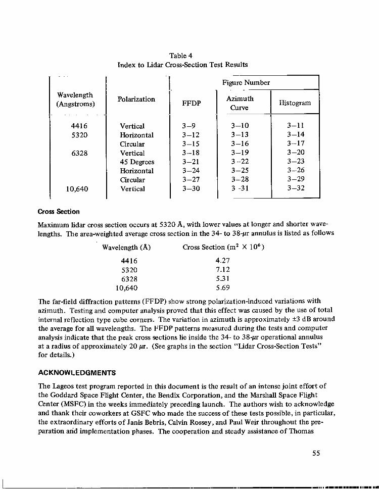
Table 4 Index to Lidar Cross-section Test Results

Wavelength (Angstroms)

441 6 5320

6328

10,640

Polarization

Vertical Horizontal Circular Vertical 45 Degrees Horizontal Circular Vertical

~ ~~

FFDP

3 -9 3-12 3-15 3-18 3-21 3 -24 3 -27 3 -30

Figure Number

Azimu tl Curve

3-10 3-13 3-16 3-19 3 -22 3-25 3 -28 3-3 1

I Histogram I 3-1 1 3-14 3-17 3 -20 3-23 3-26 3 -29 3 -32

Cross Section

Maximum lidar cross section occurs at 5320 A, with lower values at longer and shorter wavelengths. The area-weighted average cross section in the 34- to 38qr annulus is listed as follows

Wavelength (A) Cross Section (m2 X IO6)

4416 5320 6328

10,640

4.27 7.12 5.3 1 5.69

The far-field diffraction patterns (FFDP) show strong polarization-induced variations with azimuth. Testing and computer analysis proved that this effect was caused by the use of total internal reflection type cube corners. The variation in azimuth is approximately +3 dB around the average for all wavelengths. The FFDP patterns measured during the tests and computer analysis indicate that the peak cross sections lie inside the 34- to 38-p operational annulus at a radius of approximately 20 pr. (See graphs in the section "Lidar Cross-Section Tests" for details.)

ACKNOWLEDGMENTS

The Lageos test program reported in this document is the result of an intense joint effort of the Goddard Space Flight Center, the Bendix Corporation, and the Marshall Space Flight Center (MSFC) in the weeks immediately preceding launch. The authors wish to acknowledge and thank their coworkers at GSFC who made the success of these tests possible, in particular, the extraordinary efforts of Janis Bebris, Calvin Rossey, and Paul Weir throughout the pre- paration and implementation phases. The cooperation and steady assistance of Thomas

55

Zagwodzki, Don Premo, and Jack Coble is also gratefully acknowledged. The sometimes painful formalities of intercenter activities were minimized due to the efforts and continuous help of William Johnson of MSFC and Robert Spencer of the National Aeronautics and Space Administration Headquarters. The funding resources to carry out this work were supplied by Chris Stepanides, GSFC, whose early recognition of the importance of these tests was instru- mental to their genesis. We are also most grateful for the performance and enthusiasm of the Bendix Corporation team led by John Bruger.

Theoretical analyses of the Lageos array by computer were performed with the assistance of the Computer Sciences Corporation (CSC). These analyses proved extremely useful in anti- cipating potential problem areas. In addition, CSC provided the technical documentation services for this report. Members of the CSC programming team to whom we are particularly indebted are John Kirk, Myrna Regardie, and John Zimmerman.

Goddard Space Flight Center National Aeronautics and Space Administration

Greenbelt, Maryland July, 1977

56

REFERENCES

1. Siry, J. W., “The Lageos System,” NASA/GSFC TM X-73072, December 1975.

2. McGunigal, T. E., W. J. Carrion, L. 0. Caudill, C. R. Grant, T. S. Johnson, D. A. Premo, P. L. Spadin, and G. C. Winston, “Satellite Laser Ranging Work at the Goddard Space Flight Center,” NASAlGSFC TM X-70948, July 1975.

3. Minott, P. O., “Measurement of the Lidar Cross Sections of Cube Corner Arrays for Laser Ranging of Satellites,” NASAlGSFC TM X-70863, September 1974.

4. Zurasky, J. L., “Cube Comer Retroreflector Test and Analysis,’’ Applied Optics, 15(2), February 1976, pp. 445-452.

5. Minott, P. O., “Design of Retrodirector Arrays for Laser Ranging of Satellites,” NASAlGSFC TM X-70657, March 1974.

6. David, I. B., “Communications Under the Poisson Regime,” IEEE Transactions o n Infor- mation Theory, 15(1), January 1969, pp. 31-36.

57

APPENDIX A

ANALYSIS OF LAGEOS USING RETRO PROGRAM

An analysis of the Lageos array performance was done using the RETRO program, which was developed at GSFC for the analysis of cube corner arrays. The results of this analysis follow.

In the analysis procedure, cube corners that are beyond the angle at which total internal reflection occurs were assumed to have zero cross section. In actual test, it was found that due to Fresnel reflection these cube corners actually contributed to the cross section. For convenience, the analysis was done looking at the satellite from the south pole. This makes the cube corners lie in rings of equal incidence angle symmetrical about the pole, and facilities understanding how the array works. The analysis can be (and was) done at other angles, but these add no new information.. On Unit 6, page 17,” the pole cube (No. 1) and six cube corners in a ring inclined at 10.1’ contribute nearly all of the cross section (Nos. 2-7). The remainder of the cube corners are not effective. Since the optical positions of these six cube corners lie 255 mm from the CG, the CG correction is expected to be close to this value. An exact solution of the convolution of a 60-ps (FWHM) pulse is performed on Unit 1 1, page 2,” and confirms that the peak of the pulse indeed lies at 252.5 * 2.5 mm, which is quite close to this row of six corners. The measured CG correction in this orientation was 250 mm, which is slightly less due to the contribution of cube corners operating in the Fresnel mode which are not included in the analysis.

On Unit 1 1 , page 1 ,* a FFDP for the array is computed and displayed in the same format as used in the section, “Lidar Cross-Section Tests.” A comparison of the calculated FFDP with the measured values shows a very close agreement. The peak cross section lies at the center, followed by a rapid drop, and then a secondary toroid surrounds the central maximum at a radius of approximately 20 to 25 pr. Cross section then rapidly falls off. A strong azimuthal asymmetry can be seen in both FFDP’s caused by the use of total internal reflection type cube corners.

The cross section at the receiver position is indicated as 0.5 t times the peak cross section, or approximately 13 million square meters, while-the minimum value at the same radius is 0.2 times the peak cross section, or approximately 5.2 million square meters. The average value in the 34- to 38-pr annulus is approximately 70 percent higher than the measured value of 5.3 1 million square meters.

*Refers to the computer printout from the RETRO program (see pages A-3 through A-27).

?AU values in the cross-section matrix are normalized to the peak value and have an implied decimal point in front of them.

A- 1

. ... ... .... ._."_."_. ,,,,. _,,

The pulse shape (Unit 1 1, page 2)* shows a slight skewing towards the spacecraft CG, but the pulse width is only slightly larger than would be predicted from a point reflector.

Unit 1 1, page 3,* shows the effect of coherence upon the position of the centroids of individual pulses. As expected, the mode occurs at the peak of the predicted incoherent pulse, but the histogram is strongly skewed causing the average CG correction to be approximately 8 mm less than predicted by incoherent methods.

In summary, the calculations show very good correlation with measurement. Because of space limitations, only one sample of the many calculations made has been shown. However, on the basis of the results, it is believed that accurate prediction of Lageos performance can be made for system parameters not covered in the test program.

*Refers to the computer printout from the RETRO program (see pages A-3 through A-27).

A-2

I

LL LL LL l A P A A A A A CG GGGG EE LL A C a P A A A A A A GG

- - -__- *" ... ..... ..... oo-. A*"-tG -GG"tEEEEECE" I A A A GC 00 . 00 -sssssssss

-no---sssssssss - SSS ss ' 00 00

GC E € 011 00 LL LLLLLLLLLLLL A 4 LLLLLLLLLLLL A A

A A a 4 GG GG EE AA GGGGCCGGGG EEEEEEEEEEEE AA GGGGGGGG EEEEEEEEEEEE

Od nOOUrxJOflOOO0 SSSSSSSSSSSS

00 ss. - . ss ooocoooooo ssssssssIs

. .~ ............... " . . . . . . . . . . . . - . . . - ... - ... - . " ... -

R E T R C I R E F L E C l U R A R R A Y PERFCRMANCE

CON NOV 29 I Y 7 6 " .. - . . . . . . . . . . . . . -. . . - ... _ . . . . . . . . . . . . . . . . . . . . . . . .

F. 0. M I N O T T c a m 722 GOCCAHD SPACE FLIGHT CENTER

PAOGRAMMCO B Y

M. ' QEFAHDIE COMPUTCH SCIENCCS CW?C'ORATION

J. KIFK . . C I J M P U T F R S C I E N C E S C I J R P O H A T I O N

J. Z I P H E R M A N C O M P U T F R S C I E N C E S C O R P O R A T I O N

GIVEN V'ALUES "" .. ....... " . . . ... . . . - ... - . .

.. " - ..... " . . - .............. - .......... -_ ..... - . . . . . . - ...

L A S E A 1 N C I Dl-NCF A N G L E S

F U L A R ANGLE I T H E T A L )

I I Z I M U T I t A N G L E (PHI L ) ........ - - ... " ....

C U H E C C R V E R T Y P E "" """"""

INDEX

E h f R A N C E PUPIL

C C N T ' I I L L IMG O I M E N S IO# "" . - "- . " . 0 1 AMETER

COAT I IJC C f l N S l A N T S N K RHO

OIHEI~AL ANGLE o F F 5 r . T . . .

0.0

0 .0

I 4550

0 . 0 0 .0

1. ,1500 1.0000

1.2500 I 2500

C I R C U L A R

C E N T I M t T E R S

ARC-SECONDS I R C - S E C l M D S AI?C-SECONDS

A-3

G I V E N JbLUES

l i 4 A h S L l T f E R C H A R A C T E R I S T I C S """"""_""""""" L A S E R W A V f L E N G l H .

G A U S S I A N P U L S F [ O N E S f D . D E V . )

FULSF ENERGY - - .

1 H A N S M l T T F N D 1 ~ C k G C N C . E

1 R A N S M I T lEI? I I P T I C A L E f - F I C I C N C Y

0.5320 MICI<OMETERS

6o.aoao P I C O S E C Q N O S

" 0 . 5 0 J IlUL E S

0.2500 M I L L I ' 7 A D I ANS

0.1100

F E C F I V E R C t I A H A C l E l ? I S T I C S j"""" -_- """ _yii__ . . - . "" - - " . .. ." . .

H E C E I V C A D I A M F T E H O . E l METERS

f I E C C : I V E R O P T I C A L ' I i F F I C I E N C Y 1 .oo

FHOTOTUHE OUANTUM E F F I C I E N C Y 0.025

hUMflER OF' 1't I t lTOEC€CfRClVS I i C O U l R F O . . .- IO. 00 . . ..

LhIT 6 PAGE .- 2

tALCUL'ATED VALt iE5 _ . . ". . . . . . - ...

.. . . . . . . . . . - . 1 ~ b b S H I T T k R C t 4 A R A C T E H I S T I C S """""""""""""

0 37 30- 1 0 JOULES

0.1.33'JD 19

0.E120D 0'.

C - 4 0 4 0 0 24 SOUARF METERS

.. .- . . . . .

WCCE I V E l l C l i A R A C T C F ? l S T I C S I""""""_

. . . . . - . " ... - ........... A A T E N M A G A l N ..- -

GEOUIRFU S I t i N A L 0 14930- I5 JLlULES

. . . . . . . . . . . . . . . . . . . Oi90700 13

PAT14 P A R A M E T E R 0.203HD-30 MtTCRS - 4

37.(i915 MICRURAD~ ANS . .

0 . 0 DECREES . . . . . _. . . " .

.. - P H O T C J ~ l . E C T ~ 3 N S / P U L S E

WARG 1 N . . . . . . . . . . . . - .. - ... 13.3 . . . . . . . - . . . . . -

10.33 1.24

". - ..

OD

U N I T 6 PCGE 3

h

- C . l 2 7 E

- U . 1 3 3 E - c . u 2 :

- c . 1.a E F , - C . 147: - 0 . I S i Z . - C . 1 9 7 E

- C . I t 3 1 5 - C . I7 2 5 - C . l 7 ) E

- C . I 9 7 E -C.I125,

' ;C . t02E - 0 . I Y 7 :

- C . c 1 2 c - - C . i l i ' -0.22 2 5 - c . 2 2 i c - C . E l 2 S

- C . 2 9 E C - c . 2 3 7 c ;

-c .247E,

- c . 2 3 7 5 - C . 2 5 2 E

-C.2tJ2E - C . 2 6 7 5

- C . 2 7 7 1 - C - 2 7 2 E

- C . 2 ? ) 2 ?

- C . 2 Y 2 E

" ' C . 1 6 2 5 -

- o . ~ a 2 ~ ,

- C . $ O ' E

- C . Z ~ ~ F ,

4 t 4 4 4 ' - ' - . t t

. . . . . . . . . . ... - . . . .. . . . . -. . - - - -

t + t 4 + + + + t t t + ~ t * * + + ~ t + ~ 4 4 ~ 4 * + 4 4 4 4 t + 4 4 4 t + t + ~ t 4 + + + * + t 4 4 + t + t t t + + + 0 5 1 0 15 2 0 25 30 3 5 40 4 5 S O

t

P R I I O A E I L I T V DCNCJI1T

0 .0 0 . 0 0 . 0 0 . 0

- ... _.

0 . 0 0 . 0 0 .0

0 . 0 0 0

0 . 0 0 .0 0 . 0

0 . 0 0 .0

0 . 5 0

0.0

. - '? - " "" -. " -

. - . . - ~

1.50 3.00 2.00 5.00 7 . 0 0

? 0 5 0 8 .00

2 8 . 5 0 35 .50

0 .0 1.00

0.0

0 . 0

0.0 0 .0

100.00

..

0.0

' . o r 0 -

" ""

Uhl T I 1 P A G E 3

.

RESERVED FOR FUTURE USE

UNIT 6 PAGES 13-16

CcIL?E CDKNER C F O S S S E C T I O N S

INCI DEhCE ANGL E:

E F F C C T I V E G'A I N *HE A

CHUS s SECT I O N

2 3

O P T I C L L DELTA R .. OELTA R -

I C E G A C E S )

Id. 1 I 8 10.1 l e

10.1 IU 10. I 1 E

1s. c s e

1 5 . E 4 E . . 14. E 4 R

14. E 4e

c . 0 -. ""

10. I l e

IO. I l a . Is"F 9p _-

0.0 O.f>lBOJD-OJ 0 .o 0.0 .0-; n "" 0 . 0 0.€*18q3D-0.3 0 . 0 0 . U

0 . 0 0 . 0 . .

0 . 0

0 . 0

CL""" 0 . 0

0 . 0

0 . 0 0 . 0 0.0- - c . 0

- . C.2f5100 0 9 -

-___-

. . . . c.leoo.?fJ - 0 9

. . - . - - - .. . .

0 .0 0.1762 - 0 . 0 0 . 0

0.0 0.11 1 3 0.0

0.0 0.0

0.0

"- vi n-"~""

3s. 3 c s 3 9 . 3 c 9

0 .0 0 . 0 0 .0 0.0

0 . 0 0.0 0 37G750-03 . 0 .o 0 . 0 0 .0 0 . 0 0 . 0 ..._ - .. . .. - 0 . 0 - 0 .0 0 . 0

0 . 0 c . 0

.a

- u . II U.U

. . C.412130 0 9

. 0 - ." .i,. 3CS 0 .0 3'9. 3 CF ?F. IO4

0 . 0 0.0

39.2CF 0 . 0 3'3. 3 c 5 3%. 3 L F

0 .v 0.0

39.304 39. 3CF

0 . 0

3s. 3 c 5 ' Q i O

0.0

0.0 0 . 0 6.0 0 . 0 C . 0 0 .0 0 . 0

0 .0 "" - - . .

0 .0 "--a. 0 0.0

0 .0

0.0 0.0 0.0 0 .0 0.0 0 6 0 ' - - 0 00 0.0 0.0 0.0 0.0 0.0 0.0 0.0- 0 .0

. . 0.3663

- . . . . . . - . . . . . . . .

_. .. .

-0.2366 0 .0 -0.7366 0 .O

-0.2366 0 00 -0 2 366 -007366

. - 0 e 2 2 2 7 0 00

-0.2366 0 .O

-0.2105 -0.2105 - . . 0.0 . _ _ -0.2105

0 00 . . . " "oi*(05 0 .O

0 10""" -0.2105 -0.8105

0 00 0 .O

-0.P 105 0 00 -0.2105 0 00 -0.2105 0 .O -0 .2105 0 .O -0.2105 0 00 -0*2 ,03 ... " . O i 0 . " . .. -0.2105 0 .O

~ r 2 3 6 ~ O ' ~ b - - - -

. . . .

U N I T h PAGE I7

39.3CS 0.0 C O O 0.0 -0.E105 0 .O 39.3c5 ..- . 0 . 0 . . 0 . 0 0.0 -0.7105 35.3G9 0 . 0 0 . 0 0 .0 -0.2105 39.3c9 0.0 0 . 0 . 39; Jtl. V.U 3Y. 3c4 0 . 0 0 .0 0 . 0 -l l .?105 45. CJF 0.0 .. . . .. C . 0 0 .0 - 0 . I 7 H 4 45. c z s 0 . 0 0.0 0 00 -0.1704 0 .O 45. c 2 s 0.0 C.0 0 . 0 -0.1784 0 .O 4s. 635 0 .0 . : ." . - 0.0 0. 0 -0.1783 . . 4 5 . C'5 0 . 0 0.0 0 . 0 - 0 . I784

45. C35 0 .0 C O O 0 . 0 -0 .1783 0 80

4s. c 2 s . 0.0 . "" 0.0 0 . 0 -0.17H4

45. c 3 5 0 .0 0 .0 0.0 - 0 . I 7 8 3 0 .O 45. C35 0 . 0 C . O 0.0 -0.1783 0 .O

..., 4s. cz5 . .. " - 0 . 0 . . . . ". 0.0 - 0 . 0 -0.1703 - -0.0 . 4s- c3s 0 . 0 ,

0.0 0.0 "0 I783 0 .o 44. c 2 3 0.0 0 . 0 0 .0 -0. I783

- - ... qc- ~~~" ". ore""-- nio- .. - -- - . - o i l 783 oiu . 44. c25 0.0 0 . 0 0 .0 -0.1783 0 .O

4s. c i 5 0.0 c . 0 0.0 -0.1784 0 .O 45. C 3 Y 0 .O 0.0 0 .0 - 0 . I783 4s. c35 0 466.330-04 0.4 15460 09 0.01 <I4 -0.1 704 e$. c35 0 . 0 0.0 0 . 0 -0 . I784 0 .O 4G. c 1 4 0 00 c . 0 0.0 -0.1783

'atrt35- Oil) .O oiu .ioi11a4 - 0 - .0" 45. c25 0 . 0 c.0 0.0 -0. I784 45. c 3 9 0.0 0.0 0.0 45. c 3 5 0.0 0.0 0.0 4s. (39 0.0 0.0 . 0.0 -0 . I784 5 € . l e 5 0 . 0 - 0.0 0.0 -0.141 I SF.. 7 e 9 0.0 c . 0 0 . 0

5c . I C 9 0 .0 0.0 0 . 0 5L. 7 6 5 0.0 0.0 0.0 -0.141 I sc. 76s 0.0 c . 0 0.0 - 0 . 1 4 1 I

5E. 7 6 5 0 . 0 a.0 0.0 -0 .1411

0 .O 0 00

0 . 0 -0 .2105 0 -0

0 .O .o .O

~u~ ~

" " - mi 2 t 0 7 - . 0 ' 5 7

0 .O 0 .O

45. c 3 s 0 . 4 ~ 6 . 3 3 ~ 0 4 0.4 14460 09 0.01 93 " ." .. ;o.1783 "0. I 7 H 4 -0 io-.. - 1 6 I 9 " ~ .. 35. c 3 ~ O T O os* - "" "- - io

0 80

" = ~ . ~ " "" . - . ." - ". . 0 .O .. -

- 0 5 . C3F __ 0 . 0 . 0.0 - . .... " . - 0 . 0 - 0 . I 7 R 4 0 .O

0 .O

. .

-0.1619

0 .O

0 .O -0.1783 0 00 -0 . I784 0 .o

0 .O 0.0

- 0 . I4 I I 0 .O -0.101 I 0 .O

0 i o -0. I 4 1 1 0 .O

0 00 0 .O 0 .O 0 .O 0 .O

-0 .191 I 0 00

-0.141 I 0 .O

, _. - " . - . " ~

5 € * 769 0.0 0.0 0.1) St'. 7 6 5 . - oio 0 . 0 -0 . I 4 t 1 - .

S C e 765 0 . 0 0.0 0 .0 -0.141 1

SL. 7 6 5 0.0 0.0 0 .0 - 0 . I41 I 5 C e 1 6 5 0.0 0.0 0.0

. 9c; 7 c 9 0 .O 0.0 0 5 w . . . . . .--01(41 I - . . - .. - . - Q & O -. . 5E. 7 6 9 0 . 0 0 . 0 0 .0

U N I T 6 PAGE 18

? U

0 . . . .......... CUeE CQAhER CfiOSS S E C T I O N S ' . . . . . . . . .

COBE I N C l DEhCE CUkNER LNQ- L

EFFECT I VE ARE A " . " SECT I O N DELTA a - O E ~ T C - 6 " . -.

(METERS X 10 I (CETERS) [METERS)

.... . . . . . . . d~ IN CROSS bPT1CIL

I D E G R E F S ) (MCTERS 1 2 2 6

- " -. - -. 5E. 7 ~ f 0 i o (r"- ." "_ " ~ - ." o;-n" "" "" -0 ; f 4 1 ' l s U " ; 0 - I 02 5 t . 7 6 5 10.3 5 € . 7 f %

0 . 0 0 . 0 0.0 -0 .141 I 0 . 0

0 .O

104 . . Q.0 "."

5f. 7 € 5 0 .0 . - .- - r .P .141 1 4.4

I 0s 5 c . 7 c s 0 .0 0 . 0 0 .0 -0.141 I 0 .0

0 .O

I O r , 5E. 7 h 5 0.0 0.0 ... ........ 0.0 -0 .141 I 0 00

I 0 7 . . . . . - 0 . ( 4 1 1 . -0.0 0.0

5E. 7 6 4 0 . 0 1 Vf4

0 .0 5f 7 1 5 0 .0

0 . 0 C O O

-0 .141 I 0 .O

105, . . . . 5 E i 1 6 9""- o.;v - 0 . 0 -0.101 I O~-n""----- -

Q oQ

I 1 0 5 t . 7 t 's A I .*, t". v;o~"--

0 . 0 1 I 1

0.0 5E. 7 1 9

0.0 c. 0 -0.14 I I 0 .Q

11;' 5E. 7 c 9 0 . 0 6.0 -. - 0 . 0

1 1 3 s t . 7 6 5 0.0 c . 0 0.0

I I 4 . s e . 7 c s . . . . 0.0 - 0.0 -0.1a11 0 b o

I I 5 EL. 7 6 5 0.0 0 . 0 -0 . I 41 I .o -0 . . 0 . 0 0.0

11'1 SE. 7 € F 0.0 c. 0 0.0 -0.1411 0 .O

5c. i7cs """ . 'o io "*io"""p 0 . 0 - 0 . 1 4 1 1 o; (r "" -

0 00

I 1 1 1 5L. 7 6 5 0.0 -oi,*, I . "ope

0 . II 11 '1 b7. C I A 0.0

0.0 -0 .1911 0 .Q

I ;!o 6 7 . D l e 0.0 . 0.0 0.0

-0.1062 0.0

. 0.0

I ? I C 7 . C I . E C.O 0.0 - 0 . I062 6 .O

I Pi? h 7 . o l e O O U 0 . 0

0.0 0.0 - 0 . I062 0 .O

I23 61. c LE 0. u -0 . 1062 _ _ . 0-0 _ _

I 2'4 0 . 0

r37. o r e 0 . 0 0 . 0 0.0 - 0 . I062 0 00 c.n o s O 0 . 0 -0 . I062 0 .O

.. 0 . 0 I ;'tu 6 i . o l e 0 .0

"o.,06* oio I 2T

0.0 6 7 . u l e

I). 0 C.O

-0.1062 0 00

I :.!A h i . a l e 0 -0 _ _ . ._ - - 0.0 - 0 - 1062 _ _ _.__._ 0 -0 0 . 0

I 'I') 0.0

0 7 . c I e 0.0

0.0 0.0 -0.1062 0 .O

I 30 6 7 . C I n 0 .0 0.0 0.0 -0 . I062 0 00

I 3 1 6 7 . c I & 0 . 0 0.0 - -0. IO62

c.0 0 00

L X ? t,7. c l e 0 .0 -0. I Ob2

0 .0 0.0 0 00

3*" - -*,- . u I c " - ; o 1 3 4 67. C I E 0.0 . 0.0

0 s I 0 6 2 " 0 rO

I A!; 0 .0 -0. IO62

0.0 C.0 0 .O

0.0 - 0 . I 0 6 2 0 .O

1-17 6 7 . C IF ' 0 .0 0 . 0 0 .o -0 . I062 6 00

I 11 I 07 . c I B 0 .0 . . . . ... 0.0 -0.1062, 0 00

I J') 61 . c I f 0. 0

0 . I ) - 0 0 I062 0 *O

0 . 0 I40 0 7 . 0 IO 0 .o

0 .0 "0. I062 C . 9

0 00

1 4 1 0 7 i C l C - - - - oiu 0 0.0 0.0 - . - . . -0ol062 0

- 0 0 IO62 0 .O

I42 b7 . 0 If? 0.0 0 . 0 a 0 ---

1 4 3 67. 0 l e 0.0

0.0 0.0 -0 . I062 Q 00

1 4 5 h I . c l e 0 . 0 . . 0.0 -0. 1062

0.0 0 00

I45 6 7 . C 18 0.0 -0. I062 0.0

0.0 -0.1062

. 0 ; o .

I 4 f P 0 . 0

6 7 0 Cle 0.0 0.0 0 .a

I ')? 6 7 . C Ir! 0.0 0.0 -001062 0 .O

I ai4 67. C l 8 0 . 0 0 . 0 0.0 -0 . I062 0 .Q

* , . o l e . . . O e 0 - . . . . . . . . . . . . . . . 14 ' ) 0. 0

@ -0 . I062 0 .O

I !j0 16. ?st? 0 .I) c .9 060 - 0.0 -0.0624 0 00

. . . . 0 . 0

. . . . . . . . . . . . ....... ... ." . . 0 . 0 r"o;;;f . . . . . . . . . . . . . . . . . .

' f t 7 " .

. . . . . . .

. . . . . . .. . .

- . <,?. . . "I_."" ." _.. . . . . . . . . . . . . . . . . ... . . . . . -

. . . . . . . .

- 0.0 -0. I062 0 00 " v . 11 v . <I

. . . 1 10 :;: :E 0 . 0 0 . 0 "

. . . . . . 0.0

.. ............ ......

0.n

. . . . -Oi 1 oop. _" .o OO ., _. -_.

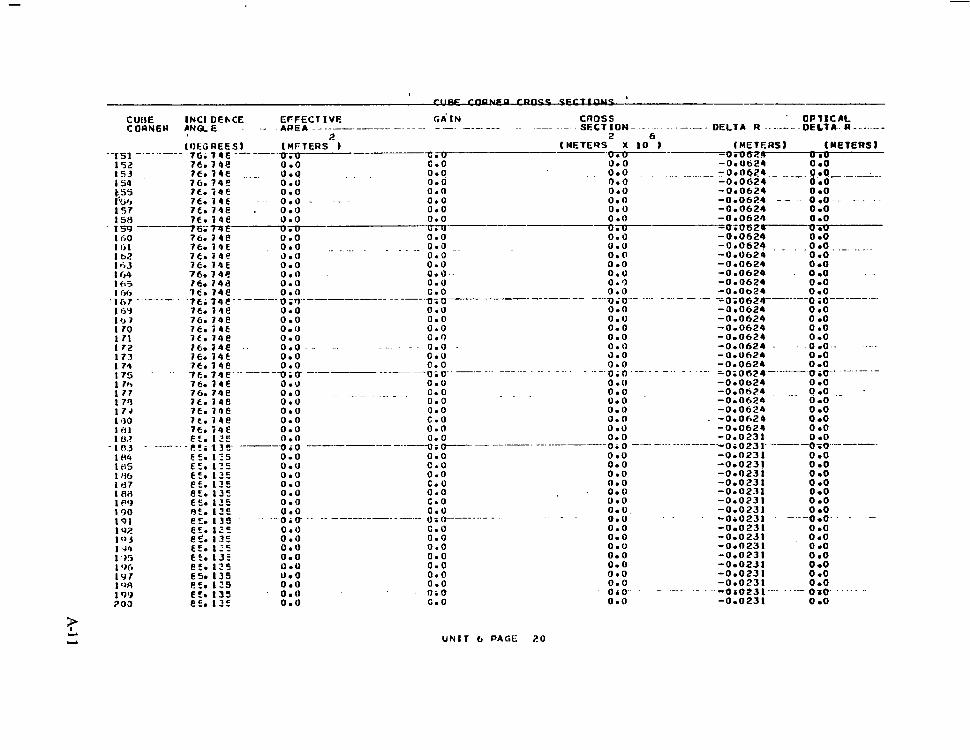
tp w UNIT I PACE 2 0

CUHF CORNER

201 . -- - ,?O? 203 2 0 4 2 05 I O6

209 2 0 7

200 ' - .' - 210 2 1 I

213 %I2

2 I4 215 s Ih 7 1 7 - '

2 1.3 2 1 7

2 '?O 7 2 1 ,? 7 .?

C U E € CORNER C R U S S S E C T I O N S '

A N U E I N C l DEhCE EFFECTIVE t~ IN

( C E S R F E S ) (METERS 1 .' EE; 135-". 0.. 0""-

A R E A CROSS SECT I O N . .

O P I I C I L DELTA R - .- - DELTA R .- -.

2 2 6 (METERS X IO ) ". o.a ( M E T E R S ) (METERS)

e:. 1 2 5 0.0 C.0 -V G 0 2 3 1" 0 r-

C E . 1 3 5 . 0 . 0 0 . 0 0 .0 -0.0231 0 .O

EC,. 1 2 5 0 . 0 0 .0 -0 .023 l--.. .-. .-.9.*L"-

e:. I 3 5 0.0 0.0

0 . 0 -0.0231 0 .O

€ 5 . 1 3 5 0 . 0 0 . 0 0.0 -0.0231 0 .o

B E . 1 2 5 . 0 . 0 0.0 -0.0231 0.0

0 . 0 € 5 . 1 3 5 0 . 0 0.0 -0.0231

0 . 0 0 00

o;r".-- 0.0 "" -0.0231 . .050231 o ~ I T ""

0 .O

E L . 1 3 5 0 . 0

0.0 . 0 . 0 0.0 -0.0231 0 .O

e:. I35 0 .o . . 0 .0 -0.0231 . . 0 .0 . . ,

EL. I35 0 . 0

0.0 0 . 0 0 . 0 -0.0231 0 00

Y 4 . E t S 0.0 0.0 -0 .0231

0.0 0 00

9 4 . € C E 0.0 - 0 . 0 -0.0231 . 0.0 . -

54. t t 5 0.0 0 . 0 0.0 -0.0231 . 0 00 0 . 0 *;"-" - oso" " . 0 00

9 4 . E e5 94 . € E5

(1.0 0.') . ._

0.0 0 . 0 ,

0.0 -0.0251 0 .O

' ) 4 . € E 5 0.0 0.0 -0 .0231

c . 0 0 .O

94. € 6 5 0 . 0 0.0 0.0 -0.0231 0 .O

94. E € 5 0.0 - . . . . . . 0 . 0 -0.0231

c. n 0 .O

94. € 6 5 0 . 1) 0 .0

94. € E 4 0.0 0 . J 0.0 -0.0231 0 00 0.0

9 4 . E C E 0 . 0 0 . 0 9 4 . € C 5 0 . 0 . " . . . 0 . 0 9 4 . € E 5 0 . 0 0 . 0 0 . 0 94. € E 5 0.0 0.0 9 4 . c c 5 0.0 0 . 0 9 4 . € C S 0 . 0 0 .0 S Q . € E 5 0 . 0 0 . 0

- - 3 1 ; € C f - - _ _ UIV"" u . w Qi-V-"""" - 0 ~ U 2 3 1 " O ~ O " ~ $4 . E € ? 1 4 . E f C , 0 . 0 0 . 0 9 4 . c c 5 0 .o 0 . 3 94 . € € E 0 . 0 0.0 9 4 . F L 5 0.0 0.0 - 1 4 . E t 5 0 . 0 3 4 . c c 5 . 0 . 0

0 . 0 0.0 - .e o.

94 . LC5 0 . 0 0 . 0 Q 4 . c c 4 0.0 0 . 0 Y Q . € 6 5 0 . 0 c . 0 94. t c c 0.0 0.0

10'. 2: 2 0.0 0 . 0 1 0 2 . 2 c 2 0 . 0 0 . 0 IO:. t E 2 0 .0 0.0 102; 2: 2 . - 103.2: 2 0 . 0 0.0 0.0 -0 .0624

. . . . . . . . . . . . . . . - - .. 0.0

.. . . . . .

~'2.-.."-".lJ-- .. "3 a;lr .- "_

e:. 1 2 5 0 . 0 -

qq; fE9 - ...... o . o . " .. . ." 0.0 -0 .0231 -o."23 ,-.- Q.o ""

-0.0231 . . 0.0 .

. . . . . . . . . . . . . . F 4 . L t . S "" -.a io c;o - - ._ 0 .o -0.0231 0.0 - -. 0 .O

. -*i023t WiO'"" 0.0 -0.0231 0 .O 0 .0 -0 .0231 .., . - 0 -0

-0.0231 0.0 0 .O -0.0231 0 .O 0 . 0 -0 .0231 0 .o 0 .0 -0.0231 0 .O 0.0 -0 .0231 0 00

0 . 0 0 .0 -0 .0231 0 00 0 .0 -0 .0231 0 .O 0.0 -0.0231 0 .O 0.0 -0.0231 . . o .O . - .. 0.0 -0 .0231 0 00

0 00

0.0 - 0 0 0 2 3 1 0 .O -0.0231 0 00

0 . n -000231 0 .O o.n -0.0231 0 .O 0.0 -0 0 6 2 4 0 .O 0. n -0 .0624 0 .O

_ - - . . . . . . .

0.0 0.0 -0 .0231 0 00

.q Qi E e 9 . . . -0 i" . .- . . 0.0 O * o . . . . . . . . -0 .0231 'oi.023* ". . . .

0.0

. . . . . . . . . . oio tsO- . . . . oio.. . - " . . -9.0624 -Oi(J62@ ..... Oib 0 .O ............ 0.0

0 .O

U N I T 6 PAGE 2 1

r"c - CUUE INCl OENCE EFFECT 1VE Gh I N CROSS ' O P T l C L L C C p N F g . #N&E ....... AQE&..--".""-.-.. .... -.--..--SEcTlON . . . . . . . . . . DELTA R -.-.-.-OECTA

2 (METERS ( O t G H E E S ) (METERS X IO B (HETEAS) (METERS)

2 6

-7~"""- 7 0 3; tf Z O ' Z O - U.U -0 .D-" -0ip62* U .P "_

2 5 2 10'. 252 0 .0 0 . 0 0 .0 -0.0624 0 .O 2s 3 . 102. 2C2 ... 0.0 .................. C O O . . . . . . 2 54 lo:. 2: 2 0.0 0 . 0

0.0 "-I -0.0624- .~ 0.4 0.0 -0.0624 0 .O

2 5s IOI.2Ci 0 .0 0 . 0 0.0 -0.0624 0 .O 2% 103. %f2 0.0 C . 0 0.0 -0.0624 0 .O I ' i 7 103.2C 2 0.0 0 .0 0.0 -0.0624 0 .O %!>d IO?. 2:; 0 .o 0 . 0 0.0 -0.0624 0 .O u-. 7""" -UZOCOBt-mu ? I 1 0 101.2:2 0 .0 0 .0 0 .0 -0.0624 0 .O 261 1 0 3 . 2 1 2 , 0 . 0 . . . . . 0 . 0 . . 0.0 -0.0624 .___ ... . . 0.0

I U 2 0 2 t 2 0 .0 ' 0.0 0.0 -0 .0624 . Q.0 EG 3 102.2t 2 0 .O 0.0 0.0 -0.0624 0 .O 2 64 103.2C2 0.0 . - 0.0 0.0 -0.0624 .. 0.0 - 2 fi5 102.2: 2 0.0 0.0 0.0 -0 .0624 0 .O

0.0 -0.0624 0 .O . 2A7 . ~ . I o 3 i 2 z 2 . .- - oio6T4' o- .0" - 2(;d 102.2..2 0 . 0 0.0 , 0.0 -0.0624 0 .O

? 7 0 I O ? . 2:2 0.0 0 . 0 0.0 -0.0624 0 .O

0.0 . . -0 .0624 0.0. . 10;. 2: 2 0.0 0.0 0.0 -0.0624 0 .O

2 14 1 0 ? . 2 : i ' 0.0 0.0 103i2cL'. ...... oio ........... .... ............. 0.0 -0.0624 0 .O Di" " - _. - 'oio621"'o io " - - 2 7 6 102.2: i 0.0 0 . 0 0.0 -0 .0624 0 00 2 7 7 I O 2 . 2 E i 0.0 . . . . . . . . 0.0 . . . . . 0.0 -0.0624 0.0 E 79 1 1 2 . 5 E E 0 . 0 0.0 , 0.0 -0 .1062 0 a 0 2 79 0 .0 0 . 0 0.0 -0 .1062 2 no 112.9EL" 0.0 "0. I 0 6 2 0 .O 20 I 1 l i . P E i 0 .o 0.0 0.0 -0.1062 0 .O

nq I l i . S t 2 0.0 0.0 -0. I 0 6 2 0 .O 2 I35 11?.4€2 0.0 0 . 0 0.0 - 0 0 1062 0.0 . .

z n 7 I l i . 5 t 2 0 . 0 0.0 0.0 -0 . 1062 0 b o 2 ' I 8 I l 2 . S L i 0 . 0 0 . 0 0.0

2.80 l l r . S t 2 0 .o 0 .0 0.0

2'32 I l i . 9 L i 0.0 0 . 0 0.0 2',3 l l ' i . O E 2 0 .0 0 . 0 0.0 -0 . I062 0 .O 2'84 l lZ.ri€2 0 . 0 0 . 0 0.0

2 % I I E . F E E . 0.0 0 . 0

2 9'J I l c . S € L ' 0 . 0 0 . 0 . E99 . . 112iSCB .... .o*o . . . . . . . . . . . . . . . . . * I O .. " ol@-- ~rMlt-------Q=o------"---

.............. ...... . . .

....... . . . . . . . . . . . . .

r ~ ~ - t f 2 u r D "259 ~ -

2 6%

z . r l i 102.2.2 0.0 rO o.i 0 ; o ......... . - ...

;!61 . 102. 2 t 2 0.0 0.0 0.0 -0.0624 0 .O

2 7 1 10:. 2: i 0 . I ) 0 . 0 0.0 -0.0624 0 .O 272 103.2! 2 0.0 . . -0 .0 2 7 3

275 - -

....... . . . . . . . . .

. . . . . . . .

11?.9E2 0 .0 0 . 0 1

0 .O

2 d;! I l i . S t 2

010 0 . 0 p; 0.0 .... ........ -0 .1062 ........... 0 .O .

2 811 I I ; . F C Z Q.0 0 . 0 '0.0 - 0 . I 0 6 2 0 .O

-0.1062 0 .O

-0 . 1062 0 .O . - 0.0 -0. I 0 6 2 .

" . 0.0 -0. I 0 6 2 0 .O

-6 .1062 0.0' . .

. ;19J ...... Ili.YtZ .......... ......... . o*2 0 . ' * .O"

z 49 I I $ . S L ' 0.0 0.0 0.0 -0 .1062 0 .O .................

2:11 112.982 . - io . ." . " - " "" @-

2 Y? l l i . S € 2 0 .0 0.0

2 17 I l f . 9 ' 2 0.0 0 .0 0.0

300 1 1 2 . ~ e 2 0 .0 0.0

0.0 -0.1062 0 .O 0.0 -0.1062 0.0

-0 . I 0 6 2 0 .O 0.0 -0.1062 0 .O

0.0 ' -0 .1062 0 .O

. . . . ... .

.........

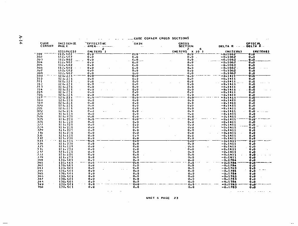
CUBE C C A N E P

"

ti 1; li 12 li li li

12 12

I2 I2

1 2 li

1;

1. 1.

I . 1. 1. I . I . t i

1. 1.

1. I .

" "

0.0 0 .0 0 . 0 0 .0 0 . 0 0.0 0 . 0

0.0 . c * 0." 0 . 0

.IT;-- U. 0 .0 a.

C. 0 C . 0 0.0 0 . 0

0.0 . . 0 . 0 0 . 0

0 . 0 0 .O

0 . 0 0 . 0 f) . 0 0 . 0 O . J 0 . 0

. 0 .0 . . .

"

_. 'o io . 0 . 0 0 .0 0 . 0 3.0 0 . 0 0 .0 0 . 0

diQ 0 . 0

0 .0 0 .0

0 . 0 0.0

0 . 11

0 . 0

- . . ." -.

a . o

0 0

"

0.0 . 0 . 0 . . 0 . 0

.

0 . 0 0 . 0 0 .0 0.0

' 0 ; 0 - 0 .0

-

0 .0 0 . 0 0 . 0 0 . 0 . 0 . 0 0 . 0

0.0

0 . 0 0 . 0

0.0 . 0 .0

0 . 0 0 . 0

0 .0

-os "" ...

. .o 0 o.-. . . .. . . .. . - .

0;0 0.0 0 . 0

0 .0 0.0

0 . 0 0 s V" - - 0 .0 0 . 0 0 IJ 0 .0 0 . 0 1) . 0 0 . 0 0 . 0 - . 0 . 0

. -. . . - .

-0.1 ." -0. - I

- 0 . I

-0 . I - 0 . I

-0.1 O h ? 0 .o -0.1062 0 .o

. . - 0 . -0 . -0 . -0 . -0 .

x Q - 0 .

-0 . -0 . -0 . -0 . -0 . - 0 . - 0 . - 0 . - 0 .

. - - . -

- .

I I I 1 I

1 I

I

1 I

I I

1 I 1 I

4 i I __ 4 1 I 4 1 I 4 1 1 . 4 1 1 4 1 1 41 I" 4 1 1

4 1 1 4 1 1

. 4 1 I 4 1 1

1411 141 I 101-1"' 141 1

. .0 .0 0 .O 0 .O

0 .O

0 .O 0 .O

0 .O

0 .O

-0 io"' 0 .O

0 .o

. . .

"- * i'u ..

.. 0.0 - _ _ - _ _ . - -.

0 .0 0 .0

0 .0 0 .0 . . -0 .1411 . 0.0 c . 0 0 .0 -0.141 I 0 .0

0 .O

UTV 0 . 0 -00 1 4 1 I 0 .O

0 . 0 0.0 - 0 . l r ) l I 0 .O 0.0 0 .0 0 . 0

-0 .1411 0 .O

0 . 0 0.0 - 0 . i 4 1 1 0 .O 0 .0 -0.141 I

0.0 - 0 .0 0 .O

0.0 -001411 - . 0.0 . . - .-

0 . 0 0 . 0 0.0

-00141 I -0 . IF84

0 .O 0 -0

0 . 0 0 .9 -0 . I 41 i 0 .o "US"" -o-i,$l,".uio."""

- ". .";,, . - " -" L. ""

0 . 0 0 . 0 0 .0 .

0 . 0 0 .0

0 .0 0 .0 0.0

0 . 0 0 .0

0 . 0 -6. i 704

0.0 -0. I 784 0 00

0.0 0.0 0.0 -0.I.783 0 .O 0 .O

0.0 0 . 0 0 .0 0 . 0

-0 . I703 0.0

0 .O 0.0 -0.1 784 0 .O

0 .0 0.0 0.0 -0i.I-783"- -0.1783

0 io- 0 .O

" O.O " . . 0 i'l784"" 3.iQ"" -0 . I 784 0 .O

. . -0.1 7e3 . 0 . 0 . _ _ _ _ _ . . .

. . _ " - - "" .. _. - "_ OTO "" "" " . - ". ." - - .-

_. - . . . . . . . .

U N I T B PAGE 2 3

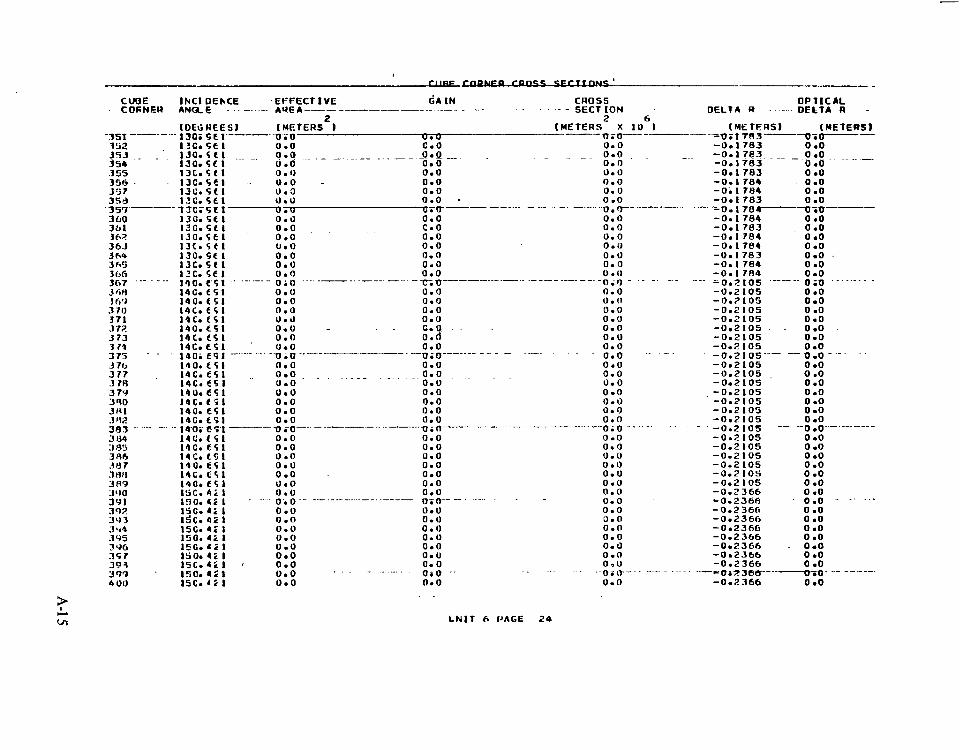
.3 71, 3 77 3 tu 3 7V 3 Y O

isc. 4; IdC. 4i ISC. 4 2 I50.4i I C C . 4 2 ISO. 4i 15C. 4 2

15c. 4 z 15a. 4;

0.0 0.0 .... ... - . 6 .o

.. 0 . 0 - 0 . 0

0.0 0.3

. -.

0.0 0.0 0 .0

0 .0 0 .0 . . 0.0 0.0 0.0

0.0 0.0

".

.- 7 . u " -. - - - - . . - " - - . - - - 0 . 0 0 . 0

u. 0.0

0 .0 0.0

0 .0

0 . 0 0 .0 0.0

0 .0 0.0

0.0 0.0 0.0

0.0

oio ".o 0 .0 0.9 - . - " - - -

0.0 0.0 0.0 0.0 0.0

0.0 a. a

0 . 0 0.0

0 . 0 0.0

0.0 0 . 0

0 .0 . . c.y - . -

0 . d 0.0 0. 0

I 0.0 a. o - . 0 .0 .-

0 .0

-

0.0 . . c . 0 0 . 0 0.0

0.0 .~ - ..

.... .... - .

0.0

0.0 0.0

0.0 0.0 0 .O 0.0 0.0 0 . 0

0.0

-o". -

0.0

0.0 0.0

0.0 0.0

.aim 0 . 0

0. 0 0 .0 0 . 0

0 .0 0 . 0

0.0 . . . .

- ..

0.0

0.0 0 . 0 ..... o.*o" . n" " . . . . . . . 0 . 0 0 .0 0.0 0 . 0 0 . 0 0.0 0 . 0 0 .0 . . . . . . . o.a

-

0.0 0.0

0.0

0. u

o s 0 -. 0.0

a.o 0 .0

a. o . . . . . . . . . .

0.0 0.0 0 . 0 0.0 0.0 0.0

-0.0 "

0 .0

0.0 0.0 0.0 0 . 0 0.0 0.0 0.0 0.0 0.0 0.0

0 .0

0.0 0.0

0 - 0

0.0

0 . 0

. ..........

-0.1 783 0 .O

-0.1783 -0.1783

0 .O 0 .o

"0.1 l a3 . .... - .o .!, ...... - -0. i 785 -0. I 783 - 0 ; I784

." - -0 . t784-

-0 .1 783 - 0 . I784

-0.1784 -0.1784 -0. I783

- 0 . I 7 8 4 '0.2105 -0.2105 -0.3 IO5

-0.2 105 -0.2105

-0.2105 -0.2 105 -0.2 105 -0.2 105 '

-0 . I re4 .. -.

-0 .21 -0.21 -0.21 -0.2 I

- 0 . 2 1 -0.21

-0.21 ' -0.21 -0.21

05 0 5 05

0 5 05

05

0 5 05

a 5

-0.2105 -0.2105 -0.2 IO5

-0 .2 105 -0.2 IO5

-0.2366 L0.2366

0 .O 0 .o 0 .O

. ~-

-aso---- 0 .O

0 .O 0 .O 0.0 . 0 .o 0 .o o i o ......... 0 .O

a .o

a .o o .a o .a

. . 0.0 . 0 00 0 .o .. - - 0.0 "" ' . 0 .O 0 .O

0 .o 0 .O

0 a 0

". -o ~

0 .O

0 .O 0 .o 0 .O 0 .O 0 00 0 .O 0 .O

a .O

. 0.0 . . . . . . 0 .o 0 .O 0 .O 0 .O 0 .O 0 .O

-0. 0 .O

0 .O

9 . .

c

"

CURE INCI CEhCE CDGNER ANGLE . - - - -

*GAIN .-

C R O S S SECT I O N

150. 4i 1 ....... 15C.4Zl I

15c. 4 ; 1

ItiC. 4 2 1 150.4;l -. -

I h C . I C 1 1nci l f I" 160. I L 1 IhC. I f 8 ItiO. I E 1 I6C. 1: 1

" _. .

0 .0 . . . -o..a - - . . . - 0.0". .

0 .0 c.0 0.0

0.0

0.0 0.0

0 . 0 0 .0 - . 0.0

0.0 C. 0 0.0 0.0

' 3 iTT o;u ~ 0 6 0 0 . 1)

0.0 0.0 0.0 0 . 0 _._ . . . 0.0 0.0 0.0 0.0 0 .O

0.0 0.0 0.0

0 8 0 .

. "

4 04 4 03

4 05 4 OB 4 0 7 4 0fl 909' ' _

415 4 1 1 4 1 2 413 4 I4 16C. I t 1 .. 0.0 4 IS 160. 1 E 1 0 .o 416 10c. 1: 1

- 9 1 7 "' lrjti *io 0 . 0

41H 419

16C. LC, 1 0.0 IGC. 151

4 20 O I O

i 6 S . € 8 1 0.0 4 7 1 1fJC. @ E 1 0.0 4 22 4 23

1 6 C o e E 1 0.0 16s. a e 1 0.0

Q 74 ' 425

165. E € I 16c 1. "oi.u

4 26 IRC. c c c 0.0 THE SUM THF. C U M

. - 0.0 0. 0 0.0

0.0 0.P . 0.0 0.0 0.0 0.0

0.0 0.0 0.0 0.0

..... ~"QiO-""

...... . . . . . . . . . *.

0 . 0 0 .0 0.0 0.0

0.0 0.0

0.0 0.0 0.0 0.0 0.0 0.0 0.0

~ ..

_. -

( t N MtLLIClNS )

. . . . . . - . . . . " ..... L N I T 6 PAGE 25

CUBE CORNL'R COOROINATES

D ISTA~CES-METERS ANGLES-DEGREES

1 4 1 5 I c> I 7

L7b 2 7 2 'I

0.0 0 .U4 70 c.0231

-0.OE2Y

-0.022 1 - 0 . olt 7n

n.o>:q 0 .0724 0.0nco 0 .04 t7

- L . O 0 C 0 -0.04C2

- 0 . C J 2 4 - 0 . 0 a o o '0.04C2

0 . 0 0 0 0 0 . 0 4 t 2

0. I 143

0 . 1 0 2 9 c. 1zc2

0 . O ( I 7 I 0.0223

-0.0223 -0.01i71 -0.lUSJ -0.12.52 - 0 . 1 3 4 3 -G.l?€?

- = C ; 0 6 7 1 " - 0 . 1 0 7 3

- 0 . 0 2 2 3

-o .onon

a.oo(;o

0 I I 7 0 0. C75 . i ' C . 0 3 5 1

-0 .0577 -0 .01 18

- 0 . 1 3 2 7 - 0 . 0 4 5 4

- C . l ! 3 € 1 - 0 . I f c n - o . ~ r t n

R SPHERICAL C O O R O I N A T E S

C THETA

C PHI

I: T H E T A

N

0 .0 0.0459

0.0 0.0 O.04 14 0.0414 ll.0000

-0 .0414 -0 . 0 4 I 4

0 . 0 0.04b2 0.01100 0 0924 0 . 0 u 0 0 0.04b2

-0.04b2 0.31100

-0.0.124 -0.0h00 "0.0462

2o.onoo

Oi272 1 0.2678 0 .2721 I 0 . l l U 0.0 I O . I I 8 O.207R 0.2721 1 0 . 1 1 0 O.2b78 0.2721

10.110

0.2678 I O e l l H

0.2721 10.118 10. I 1 8

0.2b78 I80.000 IO. I 1 8

0.2721 0.2678

I 0 . l l f l 0 . 2 7 ? I

240.000 l O . l l U 300.000

I O . I 1 8 IO. I t 8

0.25s 9 0.2721 19.e40 0 . 0 19.tl48 3 0 . 0 0 0

19. A 4 R

0.2559 19.R4R

0.2721 1 9 . 8 4 ~ 1 0.2559

60.000 0.2721

0.255'2 19.tJ4U 90.000 19. P4R

0.2721 1 9 . ~ 4 n 120.000 19.848 0.2559 . 0.2721 19.84H 0 . 2 5 5 s

150.000 - 0.2711

19.848 19 - 8 4 t I 100.000

0 . Z t i S S 0 .2721 19.E40 710.000 19.848 I Y . 8 4 H

0.2555 Witltl " - .- 1F;ROCI"- 240 iOOO"""~ 19.848 0.2721 19.U48

0.2554 0.2721 300.000 19. A40 19.86U 19.848

0.25SY 0.2JlitJ

0.2 72 I 0 .2721

1 9 . t ~ n 330.000. 19.848

0.2306 - - 0 . 2 7 2 1 - 24.579 0.0 25.579

n . 2 3 1 ~ 25.s-79

0 .2721 29 -575) .20. on0 25.579

0.23b6 40.000 29.579

0.2 7 2 I 29.579 60 .000 O;tSr,t- - " " O ; Z 7 * * - .-.. . - . - .2s- I -

29.579

0.23bh 0.2 72 I 24.979 ~ o o . o o n ..17Y - . - - n0.000" 2s.sr9

0 .23 t~b 29.579

0.23b6 0.2721 . . 15.979 120. noo 0.2721

29.579

0 .ZJtJb 29.579

0 .2721 140.000

29.579 29.579

1c,0.000 0.23C;t.

29.579 0.2 72 I

0.23bO 0.277 I 29.575) l l 30 .000 . - . 2Y.57Y

0 .23bG 39.579

0.2721 2 9 . 5 7 9 2 0 0 . 0 0 0 99.579

"GO i t 183 - - "6~!3 t ; l , ClZTW"9 220.000 29.579 - 050 29-79

- 0 . 1323 0.236h 0.2721 2s.579 ;:a. OE 29.5 79 0.23bh 0.23Gl.1 0.2 7 1 I

29-57!] . 280.000 25.5r9 29.579 300.000

0 - 2 3 6 0 29.579

0.2 72 I 0.23Gtm . - 0.2721 - - . - - 29.579 -

29.579 340.000 320.000 29.579

0.2105 0 . 2 7 2 I 0.0 35.309 29.579

39. JC9 0.2105 - f i t + O ~ - s ~ + I T 1 9 r J O 9 - . " " 3 i ' ~

0.2 7 2 I 39.309 15.652 35.309

a .2105 0 .2721 39.309 46.957 .306---39;309

39.309 -. . 0.2105 - " 39.309 62.609

c.2105 0.2721 . 0.2 72 I 39.309 70.261

. 39.309 39.309

c.2105 0 . 2 7 % I 39.309 93.Y13 r.21os U.272 1 3a.309 109.566 . 39.309

39.30Y

0.2105 0.2105 0.272 1 39.309 1 2 5 . 2 1 A

0.272 I 39.309

39.309 0i2f-00- ~rf"---"- 535'309"""1385~2"""

39.309

0.2105 39i-309

0 . 2 7 2 I o..zr 0 5

3?. 209 0.2721 . 107.R26 39.309 39.309

39.309

0.2721 0.0 0 . 0 0.0

6 0 . 0 0 0 1zo.oon

- 0 *2CJsq-- . o;27p I - -

I 9. t34e

- .. n.2559 270.000

0.2721

__ "

I 40.e 7 0

172.174

0.0 0.0

120.000 60.000

180.000 2 4 0 e O O O 300.000

60.000 30.000

90.000

" 0.0 -

120.000 I50.000

. .. .

55.000

6 5 . 0 0 0 9 1 -000

39.000 I3.000

107.000

- 1 3 i o o r R1.OOO

I t 1.000 17.000

85.000

53.000 59.000

210.000 IO1 .ooo ."24OiOOO" 7 S i O O O

270.000 49.00C 300.000 2 3 . 0 0 0

leo.000 7.000 - -

330.000. . 0.0

ii7.000 31.000

9F.000 73.000

20.000 40.000 h O . O O O e u s o o u - ~ ~ o o o '

"" Izo.oo0 115.000-

-.

I oo.noo 21.000

140.000 160.000

89.000 63.000

. . 180.000 37.000 2 0 0 . 0 0 0 220.000 105.000

260.000 53.00C

300.000 320.000 w . o o a

i . 0 o c , 340.000----. . -69.00C

0.0 29.000

I I .ooa -e rn- .wb

2ao.oq.o . . 2 7 . 0 0 0 -

"

"3 1-am 15.652

62.609 46.951

78.261

1 OY -566 93.913

125.218 140.870 tJ6iftZ

187.826 172.174

-7svrrC- 3.000

71 .OOC _ . 4S.OOC

19.ooc 1 1 3 . 0 0 0

-. .. . 87.000 6 I m O O C 35.000

103.000 ." Y.WQ-

. _. - . .77.000

U N I T 6 P A G E 4

CrR'AEP. CUHE

C I

5 3 5 2

5 4 5 5 5 Cl 5 7 5n 5 6 0 6 1 6 % 6 3 0 4 6 5

b 7 66

6 d fiq

71 70

7% 7'1 7'1 75 76 7 7 7H 7

IO0 93

CbRT E S

0 . 2 . 3 i b

0.71311 c .22 79

c. I I l C 3 C.IPC9,

runF.n.-fllDm- D I S T A h C E S - M E T E R S ANGLES-DtGRFES

SPHERICAL C O O R D I N A T E S .". .

I A N C~ IORDINATES . . . " - -. - - . . " - - - - .. . . . . . . " . . .

R . v . ' 7 - . -

1HET.A r - -

PHI ~ . . - -0 a 0687 -0 . lonn - 0 . I 400

-0 . I bna

-0 1.324 -0 1720

-0.1530

- 0 . 0 8 9 6 -0.0465

' Z O . 1260 ""

0 . 0

- 0.2105 0.2105 0.2105 c.2105 C.2105 G.2105 0.2105 G;Z!fUB" 0.2105 0.210s . 0.1784

o.zi.7 1 0.272 I 0.272 I 0.272 I 0.272 I 0.272 I 0.272 I

0.272 I 0.272 1 "-

0.2721 0.2721

39.306 39.309 39.309 39.309 39.309

39.309 39.309

39.309 . "

3Y .300 79.309 49.039

203.<7\1 219.131 234.7AJ 250.4.15 26bmC87 28 I . 7 .3 *4 297.392 313.044" 32R 696 344.348

0 . 0

. ". .

0.0474 0.OF22

0 . i

0.1321 0.1

0 . I 0 4 8 0.1 0.1 0 il

0.2023 0.1 0.2051 0.1 0. 1968 0.1

.. .. 9 987 . -

784 0.2721 784 783

0.2771 0.2721

78 4 0.272 I 7n4-----ozt721 783 783

0.2 12 I 0.2721

784 0 .2121

4 9. O J Y 49.039

49.039 *9;03*-- 49.039 80.000 49.035) 4 9 . 0 3 Y I O C i . O b 6

93.335

49.030 - -.

001779 0 .1783 0 . 14'34 0.17R3-- - 0.7721

0.2721 49.039 120.000 4'3.03Y . 133.335

26.667 13.333

53.333 40.000

'" t 6 i 606 '.

-0.023~ - 0 . 0 7 0 3

0. I783 0 .2721 0.1783 0.2!21

-0 .1 179 0 .1784 -0 .2721

1"bsr)2"- - I I

0.2721 0.2771

I I

0.2121

I - - 0.2721 0.2721

I 0.2721 I U.2721 ," oaezrl"- - .

1 1 0.2721

0.2721

-3Ri7hQ 58.769 58. 7(>9 Sb.7'6Y 5P.709 SR.7C.U 58.7L9 58.769

. Sea7t79 . -

58.769 58 .7 t9

"

. . " . . . . .

". __

T H E T A OR

Irt - "" 35.309 39.309 39.309 39.309 39.309 39.309 39.309 39.309 " . 39.309 39.309

4 9.039 4 5.039

49.039 4 5.039 4 9.039 990 039 4 90 039 4 F. 039 4 9.039 4F.039 4 9.039 49.039 49.039

49.039 l86.66t. 49.039 45; 039"

49.039 213.333 4 9.039

-0. I 7 7 9 2lh.6h6 49.039

0.1783 002 72 I 49.039 23Y.99Cl 4 % 039 0.1784 0.2721 49.039 253.333

-0.2051 0 . 1784 49.039 2 h 6 6 b <r 4 9.039 4 5. 039

0.272 I --u-.z~zw-----"~I r ~ ~ n i + ~ ~ l - - - 4 v ~ v 3 ~ - ~ 7 ~ ; ~ ~ ' ~ ~ - - . ~ 9 9aY 39-

-0. I LIB7 -0. I 6 4 8

0.2121 0.272 I

49.039 203.333 49.039 49.039 49.039 4 S. 039 45.039

5 E . 769

-

. -. -. . .

45.1139 ? 0 0 . 0 0 0 49.0 39

-0. I 4 9 4 0.i784 0 . 5 7 2 1 49.039

- 0 . 1 3 h n

0.1784 0.17H4

5 e. 769

4 e i 7 a 9 .-- 5e.769 5 E . 769 5e.769 5e. 769 5e.769 58.769

f r e g 5E. 769

5je.769 5 € . 769

5 I .000 2S.OOC

Ll9.000 93.000 67.00C 4 I .000

" 1 0 9 ; O O U 15.00C

e3.000 57.000 I I .00c

105.000 79.000 53.000 27.000

I i O b b eo.oo0 93.333 .

9 s . 0 0 0

I 06.666 69.000 43.000

120.000 I 7 . O O C 133.331 . I 1 1.000

U N I T 6 PAGE 5 . . . . . - .

. CUBE CORNER COORDINATES'

D I ~ A ~ C E S - M E T E R S ANGLES-DFGQFES

C C R T E S 1 A h C009DlNAfES SPHERICAL COORDINATES O R I E N T A T I O N CNGLES

CCRNCR ' X 101 0 . I I Z Y -0 .2024 0.141 1 0.2721 5P. 769 150.960 se. 769 150.968 I02 -0 .2CPO 0 Ob9b 0.141 I 0.2721 58.769 ' 162.581 .

I 19.000

103 -0.23 14 0 . 0 2 3 5 0.1411 0.272 I 5e .769 174. I93 S e a 769 58. 769 . 162.581.. 93 .000

I04 -0 .23 I4 -0.0235 0.2721 5n.7tr9 185.806 5e. 769 1 ~ 5 . 8 0 6 174.193

0.141 I 67 .000

I05 -o .?z in -0 Ob96 0 . I41 I 0 .272 I 58.769 197.419 5e. 769 197.419 4 I .000

106 -0.2039 - 0 . I I PC 0.141 1 0 . 2 7 2 1 5 a . 7 ~ ~ 9 209.03.? 1 5.000

107 5e. 769

-0.1765 209.032

-0. ISIS Om I41 1 0.2721 58. 7h9 220.C145 5 E . 769 220.645 IC9.000

108 ''0.141'4 " '0.1f300 " . - 0.141 1"-0 t721""-."'5*i7f9 237iZJV" - " 5Q. 769 - . -. 232i25F"- " " ~ 5 1 ; O O r a3.000

103 -0 .1025 - C 2080 0.14 1 1 I I 0 -0.2252

0:2721 58.769 243.811 5E. 769 0 . 1 4 1 1 ...

243.P7 I -0 .O iE- I 0.272 I 58.769 255.404 58.769 755.484

3 1.000

I l l -0.01 18 -0.2.323 0.141 I 0.2721 58.7f89 2157.077 5e. 769 267.09f - s.0oc

1 I2 o.o3c,2 -C.2300 0.141 I 0.2721 99.000

C.04OH - 0 . 2 1 R 2 - 0.141 I 58.769 278.710 58.769 278.710 73.000

1 1 3 I14

'JE. 7fF9 290.322 50.769 290.312 . . - 47.00C 0.141 1 C.IL21 0.2721 58.769 30 Y -9.36 se. 769 301 -936

I15 C.160J -0 . l60h 0.141 I 0.2721 59.769 313.SQR 58.769 2 I .ooo

o . I ~ c ' I . " . . = o ; I J ~ 0.14IT""UZ27ll"- 313.548

1 1 6 -. - 5eirn9-- 1251. sei 769 - 3 2 S Z I l 2 r"""8$-.000 ' llL.OOO

117 C . F I 3d -0.0917 0 .1411 0.2721 1 I R "0.0461 .

5e.769 0.1411 . .

336.774 5 R . 769 336.774 0.2721

63 .000

I19 0.;',979 se. 769 349.347 58.769 . 348.381 . . . 37.000.

0 .0253 C.24C2 120

0.1062 0.2.3so

0 . 2 7 2 1 67.018 5. 806 0.C150

67.018 0.1062

5.806 0.277 I

63 .000

I Z I . c . 2 1 ~ 0.1216 0.1002 -- 67.01R

0 . 2 7 2 1 . - - 67.018 . 29.032 . .. 670018 17.420 67.0 18 17.420 37.00C

I22 c . 13co 0. lli 32 0.1062 0.2721 67.018 40.G45 67.018 40.645 - - 29.032. -- I I o 0 0 0

123 0. I5 5 3 0.1062 0.2 72 I 67.UlR 52.25R 67.018 52.298 79.000 I0c .000

o . l , a l

125 C . O A Z 8 0.2425 0.1062 0.2721 67.01 A 75.4.34 h7.018 75.4e4 27.000 I 2 6 131 - c . o 3 7 q 0.2470 d.'l0Ui! 9H.710 67.018 95.000 1 2 8 17v

-C.0870 I10 .322 67.018 110.328 69.000 -0.1 325

I 3 0 - C . I 7 2 6 OolHlS 0.1OcJZ 0.2721 67.018 133 .548 67.018 . 67.018 . - 121.9.36 - 67.018 - 121.936 - - - - . 450000

133.54E 1 3 1 -C.%OSi> 0.1431 0.1062 0.2721 67.018 1+5.16l 67.018 145.161 I I I .000

17.00C

I33 -C.LIEJ 0 .0504 0 . 1 O l l 2 0.2721 67.010 1Gfl.387 67.018 I 3 4 0.u000

168.3P7 -C.L:,CJ 0.1062 . . - . 0.2121 - . 67.018 .

59.000

-0.0504 0.1002 67.018

0.2721 67.OlH 1 0 1 e61 3 hl.018 - - - L91.6i3 " -. I R O . O O O 33.000

1 3b "c.2302 -0.0'108 0 . I O G 2 0.2721 67.018 203.226 67.018 203.226 137 . - 0 . 2 0 5 6 . -0.1431 - O o I U G 2 0 .7771 . - - - 67.018 .

101.000

138 -0. I726 -0 .1B15 0. I Oh2 67.010 226.452 67.018 226.452 49.000 214.e3'3 - . 67.018 214.839 - - - 75.00C

139 -0.1325 -0 2 I26 0.1052 0.2721 61.018 230.065 67.018 238.065 23.000 .,149--rtuec v . m r " - - - a r ~ o r n - - - 7 ~ u ~ ~ ~ r - - - - - e r ~ o ~ n r ~ ~ - i e r r " + t r ~ e ~ c ~ .I4" =c.c~~~--"-a~"

0.2721 . . . 142 O.Olr7 -0.250?, 0 . 1 0 ~ 2 .. . . .. . 61.018 . 212.903 . 67.018 . 272*?P3 - . . . 65.000 1 4 J 0.062H -0.2425 0.1062 0.2721 67.018 284 -51 h 67.018 284.516 I44

39.000

I45 0.1523 -C.I*tJl 67.01f3 307.742 67.018 307.742 I C7.000 I 4 f a O . 1 J C O -0.1632 0.1062 0 . 2 7 2 1 67.018 219.355 67.018 319.355 8 I .000 141

o . t l S n ' - . *UxUTSO """Qi-tOtrZ- O i + T t ~ " " - 8 7 ~ 0 1 8 """342i5Yl (r7.018 1 4 H 342~58+1-"-29~00C' 76.748 0.0 .. 55.000

CUHE n T P E T A PHI T M T A PHI GAMMA I . -. - - - - - - - . . . . c - " c - c - -. - . N N- .- .

0.2771 - 0 . IS 74

0.~24,-"--'-u;l0li2--o;27tf 67;o*8 P Y ~ ~ T I - " - - - - 6 7 . 0 1 n a 3 ~ ~ f r - - 5 3 2 u o o - 1 2 4 ' t . 1 1 0 3

0.0127 _ _ C.ZCJO? . ". 0 .1062 .. '?9?72!-...-. 67.018 .. .. . 87.097: .. " . 6 7 . o l a 98 f , b _ . 0.2721 6t.01U

0.2349 0.IOb2 0.2 72 1 67 .010 0.2116 O . l O h 2 0.2721

I37.097 I .ooo.

" t J f - " ~ t r t l t ~ - - o i v r ) n a - b c t O b Z u.% I 1- a m w n errmrJ--smrt---mzvw- 19o.onu

I35 -C.R453 ?.OOC

0.2721

1 4 1 - 0 . u 3 p -0.2476 0.1062 0.2721 G 7 . 0 1 8 ZG1.2YI 67.018 261.291 91.000

0.110.1 -0.2249 0.1062 0.272 I 67.OIR 216.12'3 67.018 296.129 13 .000

c.2190 -n.1216 0.1062 0.2721 57.018 330.969 67.018 330.968 55.000

1 4 9 0.2452 -0.0253 0.1062 0.2721 67.OlA 354.103 67.018 3540193 3 0 0 0 0 I50 C . 2G 4f l 0 . 0 0.2721 76.74B 0.0

0.1062 . -0 .2721

0.0624

w U N I T 6 P A G E G " .

\o

P tL 0

<411rESIbN COLlRI>lNAlES CUJE CCFNCR X Y . 2 - - - . c c - . c - . 1 5 1 152

fl.?'jS7 0.0'517 0.0624 0.2721 76.74t4 I I .250 0.2447 O m 1 0 1 3 O .OeZ4 0.7721 C . Z L C X 0 .1471 0.0024 0.272 I

76 -74 U 22.500 76.740 J l . 7 5 0

S P H C R I C A L C O O R D I N A T E S R - - Tt"I.TA PI4 I

I 1 0 1 7 1 172 I 7 3 I74 I75 I 76 I I 7 I 1.1 I 7 9

- 0 . o s i 7 - 0 . l O l 3 -0 .14 7 1 - C . I 173 -c . ;?2c2 -€ .2447

" C . ? 6 4 8 - -C.?S<7

-C.E5<7 - C . ' 4 4 7

0.0624 0.0624 0.0624 0.0624 0.0024 0.0624 O.Oe24

- 0 . 0 5 1 7 --0.101 3 0.0624

0.0(,24

-0.1471 - 0 . l c l 7 3

0 .0624

-0.2202 - 0.0b24

-0 ,2447 0.0C124 0.0624

-0 .2597 0 .0624

0.0517 iJ.1013 -0 .2447

-C.,75Y7 0.0629

c . 1 4 7 1 0.0629.

-0 .?%02 0. I d 1.3

0.0624

0.22C2 -0.LJ7J 0.0024 -0.1471

o."ooo.. . O l t T .

a.nuoo - ~ - . = ~ ~ ~ G w ~ - - - o ; I J G z T -

0 2447

0.1873 O-IQ7I 0 .1313 U.0517

c. 2202 0.2721 76.748

0.2721 0.2721

76.74 R 76.748

0.2721 76.748 0.2721

135.000 7h.74n

0.2721 146.250

7c. 748 197 .500 0 .2121

."Q;2721 "-78;lflW"" - 1 R O ; O Q O 7 5 . 7 4 8 l b 3 . 7 5 0

0.2721 0.2721

16.749 1'31 . % S O

0.272 I I G . 1 4 3 202.500

0.2721 16.748 213.7'30 76 .70U

0.2721 . 225.000

0 . 2 7 2 1 76.74 0 76.740 24 7.50 0 16.74H 250.750

0.2721 76.740 281 ~ 2 5 0 .. .... 0.2721 ... . . 76.740 . . 292.500

0.2721 0.2721

76.74(1 76.748

0 .2721 76 .748

_.

2 x . 2 5 0

0 . 2 7 2 1 " u ; t 7 z r - - - t e . 7 ~ ~ 1 - - Z ~ O . O O O - -

1 0 1 . 2 5 0 112.500 123.750

303.750 315.000

-. ..

- 0 . 0 1 t 1 -u.1279 -C.l?C^O - 0 . 2 3 S t i - 0 . 7 IF1 -o.:?Lis4 -0.265Y '=c.?asn . - -0 .2594 -0 .2391

" . .

_ .

0 e 0 2 3 I 0.02 1 I

0.023 I 0 e 0 2 3 I 0 . 0 2 3 I U T 0 2 3 1 0 . 0 2 3 I 0 0 0 2 3 1 0.0231 O.OL'3 I 0.0231 060231 0.0231 0 r 0 2 ¶ I 0 .02ul 0 .0231

- 0.2 721 @:e I35 0.2721 €5.135 0.2721 CS. 135

I C J I . e 7 5 163.12'5 174.375

"

- - .. . ..

76.748 70.740

76.748 76.740

16.745

I I .250 22.500

45.000 33.7EO

56.250

79 .000 3.000

57 .000 71 .OOC 45.00C

76.740 67.500 19 .000 76 .740 70.150 ."6. 7 4 8 I 13.000

76.748 70.748

101.250 6 1 . 0 0 C

76.740 I23.7E.0 112.500 35.000

9.000

905000"-. 87;000'

76.748 76.148 76 .748

Tb; 74n 76.148

76.748 76. 740

76.74H 76 .748

76.74H 76- 749 76. 7 4 H

76.74R 76.748

76.740 76.740 76.74R 76.748

" 8 % I 33- 76.749

85. I35 95 . I J 5 65. 1.15 05. I35 85.135 05.135 8 5 . 1 3 5

""?6; 790.'

146.250 135.000 I 0 3 ; o o o 157.500

77.00c 51 .000

168.750 119iOUO-

202.500 191 - 2 5 0 93.000

6 7 . O O C

* o ~ ' o o o ~

2s.ooa

2130750 ' 4 i .ooo 225 .000 15 .000 2 36.280 - IOF.000 241.500

57.00C 27uioov"--Jl-iooo' 281.250 c . 0 0 0 292.500 95.00C

258.750 83.000

- -. " - -

305.750 315.000 326.250 2 1.000

. os: 1 "5. I 0 5 . I 85.1 R 5 . I HE. I 85. I 85. I 851 1 95. I 5 5 . I

39.375 50.625 61 .875 .. - 73. I25 81.375

iiG.000 - 37.009

t3.000

I 1 .ooo 105.000

53.00C T 9 i O O O

. . 27.00q

95.00C 1.000

- - . 69.000 43.00C I7.00C

1 I I i o 0 0 85.00C 99.000

-. . . ."

_. ~ .. -

U N I T 6 P A G E 7

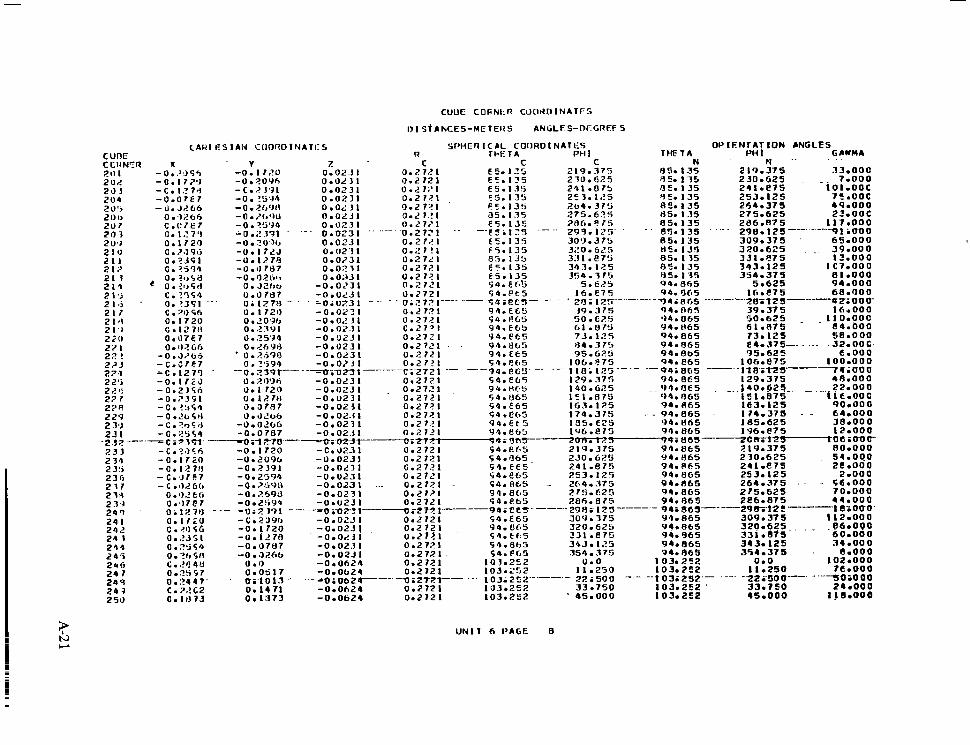
CUUE COfiNl:R CUCIhlDINATFS

0 1 S t A k C E S - H E T E H S ANGLES-DEGREF S

CUOE

2 2'3 2 39 23 I -2 .Y t 23 J 2 3 4 2 3!i 236 217 2 13 2 3'2 24 24 I 242 24 I

2 4 T1 244

24 ? 246

299 24 -J 253

:R X . Y z -O..':)C'I - 0 . 1720 0.023 I -0.17?'.) -0 . P O W 0.0211 - C . 1.174 - C . > J ' 4 1 - 0 . 0 7 E 7 -0 . ? 5 7 4 "J.3266

0.0231

0..>266 -0. 21," 0 . O i J l -O..?f,'W

C.C?E? 0 . 0 2 3 1

0.1.17'1 -0 .2 .1w - -0 .?:j'34 0 . 0 2 3 I

0 . 1 1 2 0 -0 . .? 0'31, 0.OtJl 0.0231

0.0231

c . ? ? s a 0.0787 . 0.?3FI ." Oil278 .- ' . '0.0231

-0.0231

c . 7 0 sfi 0 . I720 -O.OP?I 0;1720 C.12711 0.07C7

-0 .3 , '65 O . l l * ? G h

- C . C 7 E 7 iC.1271

."

"

- C . Z 3 9 1 , -0 . I 7 2 0 -0 . i2te -0.0787 -0.026b

0 . 0 O.OBI7

' v i 101.7 .---

0.1973 0.1471

R

0.272

0 .L 1;' 0 . 2 12

0.2 7? 0 . 2 12

0.2 7 2 0 .272 0.27?

C

- .

0.2 ?> 0.2 I ? 0.2 7 2

0.21.1 0.272

0.272 Oit77

0 .272 0.2 7 2

C.27' 0.272

0 . 2 7 2 - -. ".

S I ' H E R I C P L COIIHDINATES r k E T A Ptl I

OP I E N T A T ION LNGLES PH 1 GAYUA

N -. . . .

UNIT A P A G E 8

2 1 9 . 3 7 5 230.625 291oe75 253.125 264.375 275.625

298.125" 309.375

. 286 .n7 5

320.625

343. I25 331.e75

354.37 § 5 . 6 2 5

33.000 7.000

49.000 75 .OOC

117.000 22.00c

- i o l . o o c

""91 imo 65.000

, 39.000 13 .000

I C7.000 8 1 -000 94.000

? N N

254 255

257 2 5 6

'258 250

2 6 I 260

26 7

264 26 3

7h6 2 F. 5

2ti 7 2 l i H 2 (i 9 2 7 0 271 2 7l? 27.7 2 7 4 - ?75

277 2 ? 5

2 70 2 74 290 26 I -202 ""

29 7 -0.1726 29n

-0.1815 '0.1 525 . . * O i 2 1 3 0

0.272

?q9 ~0.-1062"" -" '0~?-72

-C.O3 7 0 300 -0.037'4

-0.2349 -0 24 76

- 0 . I Ob2 0.2 72 -0.1002 0.272

-0.10h2

1 I

I I I

I I

1 I I I I 1

. ..

. .

i 03. 103. 103. 103.

"-1 03. 103.

103. 103. 103. 1 1 2 . 1 1 2 .

-1 t2; I I e.

112. 112. 112 . 1 1 2 .

I I ? .

~~~~~

12.9c7 12.982

121.93k I33.94tl

12.Fr?2 ' - - - - - ' t q 5 ; ~ 6 1 ~ - "" 12.982 156.174 12 .9P7 168.307 1 2 . 9 e 2 180.000 l2.5C2 17.9t'2

171.613

12.982 203.22h 214.@3V

12.9622 226.45'

I

N T A

752 2 5 2 2 5 2 252 7 5 % 252 252 252 252 252 252 2 5 2 2 5 2 2 5 2 2 8 9

2 5 2 252

2 5 2 7 5 2 2 5 2 252

2 5 2 2 5 2

252 2 5 2

2 5 2 252

9P2 ,402

9rJ2 9 9 2

9 M 2 9 e2

9H2 9PZ

9 e 2

. . OH I E N l A T I O N A N G L E S

- .. .

PH I GACLIA

56.250 9 2 . 0 0 c . . 47.599 "_ _ _ _ _

78.750 66.000 4o.ooc

90.000 14-000 101.250 . 1oe.ooo I12.500 02.000 123.750 5 0 - 0 0 0

7 3 5 ~ w 0 ~ 0 0 - 146.250

, 157.500 4.00C

168.750 . qe.000

180.000 46.000 72.000

191-250 -. 20.000. 202.500 I I4.OUO 213.750 RR.OOC 't25i000 236.250

B t i O O t -

247.500 36.000 I c.000

270.000 258.750 I o4.onc

. . . 281.250- - - - - -52.000 70.000

292.500 303.750

26.000 120.000

3 t 5'; 00 0""-- 326.250

9 4 5 0 0 0 - 68.000

. 437.501). . . . 42.00c. 346.750

5.806 16.000

I I 0 . 0 0 U

29.032 17.420 e4.ooc 40.645

5 8 . 0 0 0 32.000

63.871 1 0 0 ~ 0 0 0

87.097 74.000 48.000

. - _. . . " R"" " ' ' . "

"

?!2rZJE-"" e i o o c - 7 5 . 4 8 4 .

203.226 214.839 226.4E.2 - - ..2~"io*s . .-.... 249.617 261-291

UNIl 6 P A G E 9

CUUE CCGNEP COORVINATES

DIST'AhCES-METERS ANGLES-DEGREES

C A R T E S I A N COORDINATES S P H E R I C A L COORDINATES f l R I E N l A f l O N YHiLES R THETA T M T A PH I GAYMA "~

PHI " ..c- - "" ". "_ -. - c c RNER'

CUHC

30 1 302 303 304 305 30h 301 309 309

3 1 1 3 1 0

313 31%

314

' 3 I 6 315

317 310

3 20 3 1 9

3 2 1 3 1 2

324 32 3

325 326 -12 7 329 32 4 330

7 3 7 - 33 I

334 33.3

335 336 33 1 Y 3H

3 4 0 .. 339

3 4 I 34% 34 3 34 4 345 346 34 7 34 E 34 J 350

0 . 1 2 2 1 C e O H C H - 0 i O 3 E 2 "-

- C . O 5 i t J

-0.1424 -c.10i5

-C.l?€S - C . ? 0 3 4 -0.2220

-0 .2 .1 14 - 0 . 2 2 2 0 - 0 . 2 0 2 4 - C . l ? r . S

-C.lOi5 - C . 1424

- C . O f i t l l -C<DI lr)""

C . 0 3 E 2

c.1721 C.0dCB

C . 16OJ

-0.01 I ?

- -C.2310-."

"

0 . i s74 0.21t12

-0 .141 I -0.141 I

0.2721 0.2721

121.231 121.231

5H. 065 69.677

121.231 121.231

58.065 69.617 1oe.ooc

14.00C

us141 t" 0 i Z Tft" 3ts+96"*2t-.-2Jt--

0.1515 -

0 . 069tj 0.1 12')

-0 .OZL15 0 G OZ3ET"

." .. - 0 . 1 4 1 I 0.2 72 i -0.1411 - 0.2721

121.23

-0.141 I 121.23

0.27ii .

- 0 . 1 4 1 I 0.>771 lil.22 121.73

-0 .1411 - - - - 0 . 7 1 2 1 -- - - -121.23

-0.141 I - 0 . 1 4 1 1 0.2721 12 I e23

0.2721 i u.Z7+t"ft1;23

121.23

-0.141 1 0.2721 12 1.2' -0.Ob96 . - 0 . 1 4 1 I _ _ . 0 .2721 . .. 12 1 e 2 3 1 -0 .1129 -0 .14 I I 121.221 2 0 9 . 0 3 2 121.231 200.022

107.41Y .. 1210231 _ _ _ 197.419 62.000 O . Z ? Z I

- 0 . 1 5 1 5 -0.141 I 0.2721 121.231 220.645 1210231 220.645 36.000 10.000

-0.11140 -0.1411 . . 0.2721 121.23 I 232.754 - - - 121 .231- - -232 .26@ 104.000 - 0 . % O H 9 "0.14 1 1

- 0 . 1 4 1 I 0.2721 0.2721

1 2 1 . 2 f l 247.871 121.231 255.484 255.484 52.000

121.231 171.231

. " ~ ~

2Q3.@7l te .000

-0. I329 " ""

- 0 . 1 4 1 1 . 0.27i i . 121.231 ." "

- 0 . 1 4 I I 37s. I f i t

0.2721 121.221 336.774 121.231 336.774 1 IO.000 121.231 . ---325.161------- . 16.009

0 . I779 0.1494 -0 .1783

" .. ~

-0.17R3 0.212 I 13U.qC I 120.000 130.56 I 1.33.333

I300FtiI 130.961

120.000 133.333

64.000 38.000 0.2 72 I

UN17 e PAGE 10

A

C A R T E S l l N C U U R O I N A T E S SPHERICAL C O O R D I N A T E S OR I E N T A T I O N ANGLES

"tCkRER" .- X CUBE

I 7"- R T" -?4-"--- 19""

35 1 -0.17 16 -0.1783 0.272 I 146.666 150.961 146.666 12.000 35 2

0.1 129 - 0 . 1 ? 3 1 C.0703 . -0 .1703

1 3 0 . O 6 I 0.2721 13O.q€1

JcI 1 - C . ? O 4 1 0 . 0 2 3 Y - 0 - 1783 I60 .000 . . 130.961 , . . . ! 6 0 . 0 @ 0 . 106.000

0.272 I 13J.Ybl 173.333 1300961 173.333 80.000

. . - ". . THETA PHI "" I~ -. THETA PH 1 GAMMA

"1

3 5 4

356 355

357

J 7 2 373 374 -

-0.7041 -0.lY31 - 0 . I 7 17

- 0 i1-0 27 -0.14 IO

-0.01 19 0 .0 357 C.0'3 I 9 0.1227 0.1574

0; 1 3 5 9 0.1836

0.1724

0 . I 4 7 3 c. IbC.0

-

. - " -c .o5e9

. "_

-0.0238 -0.0703

. ~ ""

-0.au51 -0.2023 -0.1887

-0 . I321 -0 . O Y 22 = 0704 71 -

0.0 .. 0.0405.

0 . 0 #\P6

-0. i 966

- 0 . 1 6 4 ~

.. ""

0 . i Z 6 0 0.1530.

-0.1784 0.2721 . "0. I 7 8 3 0.272 1

-0. i 7 8 4 0.272 1

-0.l7R4 -0.17t14 - 8.2121

0.275 I -n. 17n3 0 . 2 7 7 1

". "

- 0 . 2 1 0 5 :0.2105 . . 0.2721 - 0 . 2 l O S 0.272 I

130.961 130.961

"1 3 0 i 9 E t""

I40.051 100 .64 I

- t * o . t 3 t-""

"

' - PB.000. 54.000

2.00c 96 .000

1 w 5 v w ~~ ~

253.333 46.000 266.666 _ _ . l e . 0 0 ~ . 2 79.999 i12.000

, 306.666 -. . --. . .60.000 293.333 e6 .000

3 19.999 3 4 -00 0 333.333 8 . 0 0 0

t O 2 - . O O U "

15.652 . .. . 76.000

3 1.304 50.000

46.957 14.00C

62.609 - F2.000 1 18.000

40.000 66.000

1 4 5 0 0 C -

"j'46'sea" "" 0.0

370 0.023s 179 - C . 1 7 C H -0.0235 -0.2106 0.2721 140.6YI - 1B7.H%6 140.691 IR7.A26

~~ ~ .. 0.272 I

" " . i ~ o . 6 ~ 1 172. I 14

"-"" """

140.6CI 172 . I74 30.000 0 , 0 0 0

.mu -0.ljel -0 . oca7 -0.2105 0 . 2 7 i i 3tl I - C . I J 2 7 -0.1oee -0.210s 0.2721

i S O . 6 4 1 140.691 140.6YI 219.131 219.121 72 0000 140.691

98.000 " .. .. .. . .. 203.473

" ""

203.474

"TlaZ--.--"=u;Csf.,~-T~~---c;ZluJ- u . m t - tlldstift"-tJQs?n)3---14oieqi -"---.t5~;IC5"--- .*c-iooo- 39 3 -C.I)577 -0 1624 -c.2105 0.2721 1 4 0 . G 9 1 3e n - 0 . 0 1 IO "0. I 720

250.435 -C .2105

1 4 0 . h F I 0.2721

250.435 140.691

20 .00c

385 - O . O : I ~ _ I -0 . IO88 266.087 140.691

-0 .2105 0.2721 140.t191 266.0e7 .. 114.00C

346 0 . 0 7 5 3 -0 . I530 -0 .2105 0.27?1 140.651 257.392 281.73Y 140.691 281 0739 BC.0OC

.IH 7 0 . I I 7 6 "0.1260 . -C.2105 . . - -. 0.2721 - . 140 .691 140.691

313.044 257.392 62.000

38') 0.14 7.3 -0.00'36 140.6'31 313.044. . 360000

5BQ -0 .2105 0.27% I

G . I G C O -0.0465 -0.2105 140.€91 32Re6')O

0.2721 140.691 140.691 328.696

344.34rl IC.000

' f P 0 0 . 1 3 4 . 1 . 0.0. - "" " ; l n ~ ~ J ~ * ~ s ~ , ~ ~ " " . , ~ ~ ~ ~ ~ ~ " " " . " - - - 140.691 344.34e 104.000

3 Y I 0 . 1 2 t a . w s 9 -0 2366 O i ' O -- - ..

0.2121 lcJo.42, orno

150.421 20.000 40.000

150.421 20.000 52 .000

59 3 0 . 0 6 1 1 0.1163 -U.L?366 0.2721 i50 .421 150.42 I 40.000 . .

60.000 354 0.0223 0.1333 -0.23u6 0.2 12 I 150.421

ISO.421 60.000 8o.oon

3s5 -0.02J3 0.1313 . -0.3Jh6 0.2721 180.421 . 100.000 150.421 80.000 94.000

3Sh -0 .chT1 0 . I163 "0 .2366 150 .421

0.2721 100.000 . . 68.000

1'30.421 39 7 - 0 . 1 0 2 9 0.0863 -0.2366

120.000 0.2 72 I

150.421 150.421

120.000 140.003

42.000

3') A 'Oil2Ct ' ' 0 i 0459 -0.2368 """0;2721~ . 150.421 ' - 1c10iO00""-~"- 150i4tl"""-160~000--"--- 150.421 140.000 16.00C

3YW - 0 . I . I 4 3 a.oooo . -0.2366 0.2121 150 .421 I RO .000 I tC i000 . '

4 0 0 -0 .12c2 - C 045'3 -0.2366 0.2121 150.421 i?00.000 150.421 1 5 0 . 4 2 1

100.000 e4.000 200.000 58.000

7 e i o o o - 2a.ooq

120.000 3 9 2 c . 1 0 2 s 0.ORh3 -0.2366 0.2721 150.421

UNll 6 P A C E 1 1

IENTATION INGLES Pn I GAYMA - .- C C N

150.42 I 150 .47 I 1 5 0 e 4 2 1 150.421 1 9 0 . 4 1 1 1 5 0 . 4 2 1

1 h O . l E l 150.421

l h 0 . 1 5 l IGO. 1 5 1 I r i O . IS1 IhO.lCI

?20.000 32.00C

260.000 280.000

1oo.oflo 74.000

. .240.000 - - . 6 * 0 0 0 .

300.000 330.000

0.0'"" 30 .000

. 6 0 . 0 0 0 .

I20.000 90.000

340.000

. 4R.000 22.00c

116.000 9 C I O O C - 6 I . O O C

. " -. "

-

. R C . O O O 106.000

54.000 2e.000

" - 2 i o O c - s c . 0 0 0

44.000 70.00C

._ "

1e.ooc

.. " .

0. C467 0.0(300

u.0000 -0 .0462

"';O.ODOO

-0.041r7 - O . O : l 0 0

0 . 0

U.04 l . l 0.04 14

0.0000 ' ~ 0 . ' 0 4 1 4 -0.0414

70. c 729

0 . 0

160 .151 1hO.lSI 160.151 I 6 o ; t ' J I "_

Is0.000 I RO.OOO

-240ro00" 210.000

270.000 0.0000 C . 0 4 t 2 c . o r l o 0 0.047A 0.0Z 'Y

300.000 .i30.000

0.0

1HO.000 120.00I)

7 4 U i 000 - -. 300.000

0 . 0

60.000 .-

330.000 0.0

120.000 t YO. 000

86.00C

-240inuo- 300.000

300.000

. f,o.ooo - . . - - t iZ .ooo -0.0-?39 - 0 .04 3cl ; C ; O t ? 9

0 . 92 3'? c . 0 0 0 0

" ""

bC.000 34;OOO-

I.02.000 8.000

.. - .

."

c r a n n - *-A; - 2 - 1; ; a'; 3; 'E ~ " I ~ ~ B u ~ ~ L ~ U E E . R & I o ) L p " t € p H - - " - - - - - .

***********0********************************'****** ........................ ..... . .. . . . . . . . . . ....... ............... 9 b 96 ................... ................ ................ .............. .............. ........... ......... ,t 80 e o ........... ........... . * ........ ..... . . . . . . . . . . . . . . . .......... ... ..... ....... . . . " 0 . . *.* ..e. * ........ ........

P C AK NO COATlNG

CROS$SECTION A T f 0 . O J = Z . t J I 9 0 CI SQUARE MEfERS f INCLUDES EFF. FACTOR 1.00)

." - ._ .. -

___ "" . "_ -. "" " - " " - "" "-

-. - - "_ " - " 64

Q H

32

....... ...... ...... ..... . * 0-; .... *. . *. . *. +. *. * . - "" *

* * * * 4 . *. *. *. . *i. .... .... .....

. . . . . . __

...... ...... 6.1 ...... ...... ....... ....... € 4 ........ ........ ......... ............ ............ .............. .............. ................ ................

* * * * * * * * * O I * * * * ~ * * * * * * * ~ * * * * * * * * * * * * * * * * * * * * * * * * * * * * * I * * * * * * * * *

ARRAY PRINTED I N M I C R O N A O I ANS H F C l l I V E R IS A T ( 3H. 0 )

. ... .- ". ... ....................... ..... .............. ." 8 0 .............. ...........

. . . . . .

PA ................... -. .................. 96 . . . . . . . . . . . . . . . .

. q 6 ' 0 0 - 6 4 *c.. f Z ' u 1 0 " 0 .+18".32 - 4 - ~ - - C 4 - " C O ~ - 9 C , " - - - ' L ~ S C R v m m ~&~LEF------ d - r b " D t G R C t 3 0.0 DEGREES LASER ~ Z I M U T I ~ ANGLE=

"

LASEP PLANE OF POLAHlZATlON= 0.0 DEGREE4 , . . ,_ ,___

UN 11 I I P l C E I

Uh17 I 1 F A C E 2

APPENDIX B

A SECOND METHOD OF MEASURING THE RANGE CORRECTION

The Lageos array is composed of 426 cube corners, four of which are germanium and have no effects upon the visible laser reflections. The velocity aberration deflects the reflected beam by 32.77 to 38.34 pry and therefore the individual cube comers were designed with a 6.1-pr (1.25 arcseconds) dihedral offset to compensate for the velocity aberration. The far- field pattern of each cube corner is a function of incidence angle (i), azimuth of the polarization vector (r), wavelength (X), and position in the far-field pattern (described by the polar coordinates J/ and r)). If this functional dependence is known, the reflected pulse shape, the range correction, and the cross section can easily be computed by summing the contribution of each cube comer.

Unfortunately, such calculations can only be considered as a starting point because the actual “as produced” cube corners rarely conform to the specifications to the accuracy required for the calculations to be precise. However, such calculations are quite instructive in understanding the behavior of the array, and therefore a simple analysis of the array will be performed for one specific orientation.

To compute the return from an array of retroreflectors, the calculation starts with the individual cube corners. Their position and orientation on the satellite must be defined first. In the case of Lageos, if the cube corner location in polar coordinates is defined, the problem is greatly simplified because the radius for all cube corners is constant, and the position angles for each cube corner are identical to its orientation angles. This problem can be further simplified if a laser incidence direction is assumed in the south pole to north pole direction. In this case, the cube corners lie in several rings which are centered on the polar axis, and all the cube corners within a given ring have the same axial distance from the source.

The key to solving the problem is to determine the cross section of the individual cube corners as a function of angle of incidence and far-field coordinates. To do this, Lageos was placed in the FFDP test setup and this function was determined experimentally by recording the FFDP of each row individually. These FFDP’s are shown in figures B-1 through B-5. On the basis of the analysis of these FFDP’s, empirical equations for the cross section in the 32.77- to 3 8 . 3 4 ~ annulus.were developed and are shown with other pertinent parameters in table B-1 . The rows are nuinbered from the south pole (row 0) backward toward the spacecraft CG. The number of cube comers in each row is shown in the second column. In the third column, the incidence angle is listed. In the fourth column is given the optical distance from the spacecraft CG which is computed by the formula:

z = ~ , , c O s i - ~Jnl-sinzi (B-1)

B- 1

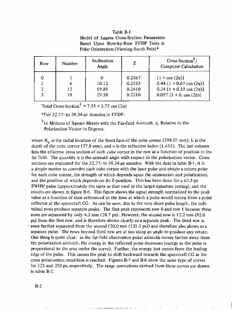
Table B-1 Model of Lageos Cross-Section Parameters Based Upon Row-by-Row FFDP Tests in Polar Orientation (Viewing South Pole)*

Row I Number I Inclination Angle

0

29.58 18 3 19.85 12 2 10.12 6 1

0 1

Z cross Section?/ Computer Calculation

0.2567

0.24 [ 1 + 0.33 cos (27))3 0.24 IO 0.44 [ 1 + 0.67 cos (277)l 0.2533 [ 1 + cos (27711

0.221 0 0.057 [ 1 + 0. cos (27))]

Total Cross Section? = 7.55 + 3.72 cos (277)

*For 32.77- to 38.34-pr Annulus in FFDP.

?In Millions of Square Meters with the Far-field Azimuth, 77, Relative to the Polarization Vector in Degrees.

where R, is the radial location of the front face of the cube corner (298.07 mm), L is the depth of the cube corner (27.8 mm), and n is the refractive index (1.455). The last column lists the effective cross section of each cube corner in the row as a function of position in the far field. The quantity 77 is the azimuth angle with respect to the polarization vector. Cross sections are evaluated for the 32.77- to 38.34-pr annulus. With the data in table B-1, it is a simple matter to convolve each cube corner with the laser pulse and obtain a return pulse for each cube comer, the strength of which depends upon the orientation and polarization, and the position of which depends on its Z-position. This has been done for a 62.3-ps FWHM pulse (approximately the same as that used in the target-signature testing), and the results are shown in figure B-6. This figure shows the signal strength normalized to the peak value as a function of time referenced to the time at which a pulse would return from a point reflector at the spacecraft CG. As can be seen, due to the very short pulse length, the individual rows produce separate peaks. The first peak represents row 0 and row 1 because these rows are separated by only 4.3 mm (28.7 ps). However, the second row is 12.2 mm (82.0 ps) from the first row, and is therefore shown clearly as a separate peak. The third row is

. even further separated from the second (20.0 mm (133.3 ps)) and therefore also shows as a separate pulse. The rows beyond third row are at too steep an angle to produce any return. One thing is quite clear: as the far-field observation point azimuth moves farther away from the polarization azimuth, the energy in the reflected pulse decreases (energy in the pulse is proportional to the area under the curve). Further, the energy lost comes from the leading edge of the pulse. This causes the peak to shift backward towards the spacecraft CG as the cross polarization condition is reached. Figures B-7 and B-8 show the same type of curves for 125 and 250 ps, respectively. The range corrections derived from these curves are shown in table B-2.

B-2

Table B-2 Peak Detection Range Corrections

~-

Azimuth Angle

0" 45" 90"

. -

. .

Range Corrections (ps) for Pulse Widths*

62.5

-1 690 -1 690 -1610

125 " - -

-1 670 -1 650 -1 620

___. ~-

I

250

-1 660 -1 650 -1610

Range for Pulse Widths*

62.5 - " - - . . . . .

-253.5 -253.5 -241.5

"

-250.5 -247.5 -243 .O

*Pulse widths are defined by ps (FHWM) units.

To compare these calculations with data taken in the target signature tests, figure B-9 was made taking the photomultiplier tube response into account. The laser pulse has a Gaussian profile and a FWHM of 62.5 ps, and the photomultiplier has a 10- to 90-percent rise time of 150 ps. When these are combined (assuming a Gaussian photomultiplier impulse response), an effective Gaussian impulse response with a standard deviation of 92 ps (217-ps FWHM) is obtained. Due to the broadening of the pulse by the photomultiplier, all indication of the separate rows is lost. However, the polarization effects are still quite evident, amounting to a shift of approximately 6 mm for peak detection. If the detector uses 50-percent peak on the leading edge as a criteria, the shift increases only slightly to 6.5 mm.

It should also be noted that the range correction is a function of pulse length. When the laser pulse is convolved with the satellite response because of the skewness of the satellite response curve, the peak of the return pulse shifts towards the spacecraft CG. Figure B-9 shows the effect for the 0" polarization conditions for pulse lengths varying from 62.5 to 1000 ps. Table B-3 shows the positions of the peaks for the various pulse lengths.

In summary, on the basis of analysis derived from actual experimental FFDP, the range correction varies by as much as 8.5 mm with polarization and by up to 8.1 mm with pulse length. The actual value derived from target signature tests (249 f 1.7 mm; see figure 18) agrees extremely well with the results from FFDP tests (figure B-10 and table B-4). In comparing these results, it should be kept in mind that the tests were taken over the entire annuius and represent an average range correction. Table B-4 lists the range correction as a function of far-field azimuth. When this table is weighted according to the relative intensity of the various far-field positions, an average range correction of 247.0 mm is obtained. The final result is that for all polarizations and pulse lengths, the range correction is 249f,o, mm for peak detection.

An analysis of figure B-10 also shows that the expected pulse width is 261-ps FWHM and appears to be in close agreement with the results. The slight increase of 21 ps (8 percent) over the experimentally measured value is probably due to the fact that the analysis was done for one special orientation, and errors in estimating the pulse width and photomultiplier rise time.

.

B-3

Table B-3 Range Correction as a Function of Pulse Length

Pulse Width

Range Correction

(PS FWHM) (mm) (PSI

62.5 -1 654 125

-253.8 -1 692

-246.0 -1 640 500 -246.9 -1 646 290 -248.1

1000 -1 638 -245.7

Table B 4 Peak Detection Range Correction

(Photomultiplier Response Included)

Range Corrections for

(PSI (mm)

Azimuth Pulse Width 62.5 X sec (FWHM) Angle

O0

-243 .O -1 620 90' -247.5 -1 650 45O -249.0 -1 660

.

B 4

Figure B-1. FFDP of the Lageos Satellite's south pole (laser type: neutral density = 0.3).

I I

I I

Figure B-2. FFDE of first row from south pole (laser type: neutral density = 1 .O, incidence angle = 10.1O).

B-5

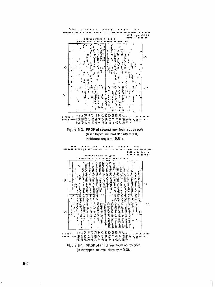
Figure B-3. FFDP of second row from south pole (laser type: neutral density = 1 .O, incidence angle = 19.8O).

Figure B-4. FFDP of third row from south pole (laser type: neutral density = 0.3).

B-6

Figure 8-5. FFDP of full satellite illumination from south pole (laser type: neutral density = 1 .O).

B-7

1 .o

0.9

0.8

0.7 I k u z E0.6

t Y

a J

$0.5 - ffl w I k0.4 4 w U

t

0.3 -

0.2 -

0.1 - I

0 -2.0 -1.9

TIME RELATIVE TO PULSE FROM CG-NANOSECONDS

Figure 6-6. Pulse return curves for 62.3 ps.

0.9 - PULSE WIDTH

125 X 10-l2SEC FWHM

0.8

0.7 I I- 0 z

0.6

t; < 0.5

!2

z VI w

k0.4 4 w a

0.3

0.2

0.1

0 -2 .o -1.9 -1.8 -1.7 -1.6 -1.5 -1.4 -1.3 -


-1.1 -1 .o

Figure B-7. Pulse return’curves for 125 ps.

1 .o

0.9

0.8

0.7

I I- u W 0.6 z U t 2

20.5 a !?

1 k 0.4

-I

v)

W

W n 4

0.:

0.2 -

0.1 t

250 x 10-12SEC

-2 .o -1.9 -1.8 -1.7 -1.6 -1.5 -1.4 -1.3 -1.2 -1.1 -1 .o TIME RELATIVE TO PULSE FROM CG-NANOSECONDS

. Figure 8-8. Pulse return curves for 250 ps.

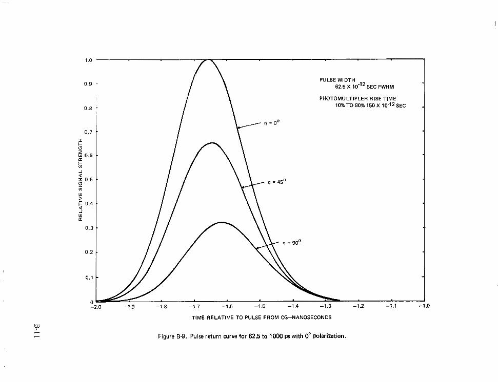
0.7 I I- (3 z w 0.6 U 5 a !?

J

Z 0.5

v)

2 F 0.4 J w U

a

0.3

0.2

0.1

0.9 -

0.8 r

1 .o

PULSE WIDTH 62.5 X SEC FWHM

I \ PHOTOMULTIPLER RISE TIME 10% TO 90% 150 X 1012SEC


Figure 6-9. Pulse return curve for 62.5 to 1000 ps with 0" polarization.

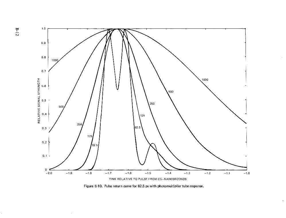
w c. N


Figure B-IO. Pulse return curve for 62.5 ps with photomultiplier tube response.

- 3. Recipient's Catalog No. 1. Report No.

TP-1062 ~ " 1'. Government Accession No.

4. T i t le and Subt i t le


5. Report Date

October 1977

723 6. Performing Organization Code

. ". . 8. Performing Organization Report Nc

G-7702 F-16 10. Work Un i t No .

5 06-20-3 3 11. Contract or Grant No.

~~ ~

7. Author(s) M.W.Fitzmaurice, P.O.Minott, J.B.Abshire, H.E.Rowe

9. Performing Organization Name and Address

Goddard Space Flight Center Greenbelt, Maryland 2077 1

13. Type of Report and Period Coverec

12. Sponsoring Agency Nom; and Address-

National Aeronautics and Space Administration Washington, D.C. 20546

Technical Paper

14. Sponsoring Agency Code

IS. Supplementary Notes

16. Abstract

The LAGEOS was extensively tested optically at GSFC during January 1976 prior to launch in May 1976. This document describes the measurement techniques used and presents the resulting data.

Principal emphasis was placed on pulse spreading characteristics, range correction for center of mass tracking, and pulse distortion due to coherent effects. A mode-locked frequency doubled Nd:YAG laser with a pulse width of about 60 ps [full width at halfmaximum (FWHM)] was used as the ranging transmitter and a crossfield photomultiplier was used in the receiver. Highspeed sampling electronics were employed to increase receiver bandwidth LAGEOS-reflected pulses typically had a width of 250 ps (FWHM) with a variability in the range correction of less than 2 mm rms. Pulse distortion due to coherent effects was inferred from average waveforms and appears to introduce less than t 50 ps jitter in the location of the pulse peak. Analytic results on this effect based on computer simulations are also presented. Theoretical and experimental data on the lidar cross section were developed in order to predict the strength of lidar echoes from the satellite. Cross section was measured using a largeaperture laser collimating system to illuminate the LAGEOS. Reflected radiation far-field patterns were measured using the collimator in an autocollimating mode. Data were collected with an optical data digitzer and displayed as a three-dimensional plot of intensity versus the two far-field coordinates. Measurements were made at several wavelengths, for several types of polarizations, and as a function of satellite orientation. Theoretical predictions of the corresponding fardeld patterns were computed and are shown to be in close agreement with experimental results. Several unusual polarization effects caused by the use of total internal reflection cube corners were noted and confiimed by computer analysis. Velocity aberration compensation methods used for LAGEOS are discussed. The array was found to have slightly lower cross section than expected, and possible causes for this difference are suggested.

7. Key Words (Selected by-Author(s))

Laser ranging, Satellites, Optical retroreflectors, Crustal motions

18. Distribution Statemcnt

Unclassifed-Unlimited

i" ?. Security Classif. (of this report) 20. k c u r i t y C l a s s i f

Unclassified Unclassified L *For sale by the National Technical Information Service, Springfield, Virginia 221 61.

NASA-Langley, 1977

F , , ''7

I ?&,

- -

':# National Aeronautics and Space Administration

Washington, D.C. 20546

I

Official Business

Penalty for Private Use, $300

THIRD-CLASS BULK RATE Postage and Fees Paid National Aeronautics and Space Administration NASA451

1 12 1 l U , D , 091977 SOO903DS

DEPT OF THE AIR FORCE AI' WEAPONS L A B O R A T O R Y

- . i BTTN: TECHNICAL L I B B B B Y ( S D L f . 1 1 KIBTEAND AFB NM 87117

Jndeliverable (Section 158 rtal Manual) Do Not Return

prelaunch testing of the laser - ilrs home page · 2013-07-18 · tech library kafb, nm nasa...

Documents