preferences recovery in address models of product
TRANSCRIPT
PREFERENCES RECOVERY IN ADDRESS MODELS OF PRODUCT DIFFERENTIATION
Weiqiu Yu
B. Sc. SHANDONG UNIVERSITY, 1983
M. A. UNIVERSITY OF NEW BRUNSWICK, 1987
THESIS SUBMITTED IN PARTIAL FULFILLMENT OF
THE REQUIREMENTS FOR THE DEGREE OF
DOCTOR OF PHILOSOPHY
in the Department
0 f
Economics
@ Weiqiu Yu
SIMON FRASER UNIVERSITY
May, 1993
All rights reserved. This work may not be
reproduced in whole or in part, by photocopy
or other means, without permission of the author

APPROVAL
Name: Weiqiu Yu
Degree: Ph.D. (Economics)
Title of Thesis: Preference Recovery in Address Models of Product Differentiation
Examining Committee
Chairman: Dr. Dennis R. Maki
h ~ r . B. Curtis Eaton Senior Supervisor
Dr. Peter E. Kennyddy Supervisor
Dr. ~oug la f l . West Professor Dept. of Economics University of Alberta External Examiner
I l ' Zs 1943 Date Approved: JvEJE

PARTIAL COPYRIGHT LICENSE
I hereby grant to Simon Fraser University the right to lend my thesis, project or
extended essay (the title of which is shown below) to users of the Simon Fraser
University Library, and to make partial or single copies only for such users or in
response to a request from the library of any other university, or other educational
institution, on its own behalf or for one of its users. I further agree that
permission for multiple copying of this work for scholarly purposes may be
granted by me or the Dean of Graduate Studies. It is understood that copying or
publication of this work for financial gain shall not be allowed without my written
permission.
Title of Thesis/Project/ExtenBed Essay
Preference Recovery in Address Models of Product Differentiation
Author: (signature
weiq'u k Yu (name)
June 2 5 , 1993 (date)
ABSTRACT
Product d i f f e r e n t i a t i o n i s a f e a t u r e of most modern markets.
The economics of product d i f f e r e n t i a t i o n has r e l i e d on two major
approaches: t h e representa t ive consumer approach and t h e address
approach. I t i s argued i n t h e l i t e r a t u r e t h a t address models a r e more
appropr ia te f o r studying most r e a l cases of product d i f f e r e n t i a t i o n .
Y e t l i t t l e empirical work has been done i n t h i s framework, due
pr imar i ly t o t h e absence of preferences recovery techniques f o r address
models.
The purpose of t h i s t h e s i s i s t o begin t h e development and
implementation of preferences recovery techniques f o r address models.
I n address models, goods a r e described by po in t s i n a continuous space
of a t t r i b u t e s o r c h a r a c t e r i s t i c s . Consumer preferences a r e def ined over
a l l p o t e n t i a l products and each consumer has a most p r e f e r r e d product
known a s h i s o r her i d e a l address i n t h e p roduc t -a t t r ibu tes space.
Aggregate consumer preferences f o r d i v e r s i t y a r e captured by a
preferences dens i ty funct ion i n some space of u t i l i t y parameters.
Preferences recovery involves t h e es t imat ion of t h e preferences dens i ty
function, given aggregate da ta on product a t t r i b u t e s , p r i c e s , and
q u a n t i t i e s sold.
The bulk of t h e t h e s i s i s on recovering preferences i n t h e
space of l o t t e r i e s . L o t t e r i e s a r e chosen because w e need "products"
t h a t can be e a s i l y c rea ted i n t h e labora tory t o genera te s u f f i c i e n t
data. Given a parametric form f o r preferences from t h e o r i e s of choice
under uncer ta in ty , w e c r e a t e a parameter space t h a t descr ibes
ind iv idua l preferences f o r l o t t e r i e s . Aggregate preferences a r e
iii

represented by a p r o b a b i l i t y dens i ty function i n t h i s parameter space.
his dens i ty funct ion i s est imated using d a t a generated from
experiments and t h e proposed technique. A test based on t h e recovered
preference dens i ty funct ion i s const ructed t o test i f a p a r t i c u l a r
theory of choice under unce r t a in ty adequately exp la ins t h e choices
people make.
Using t h i s approach, we test t h e expected u t i l i t y (EU) theory
and t h r e e genera l ized expected u t i l i t y (GEU) t heor ie s . The r e s u l t s show
t h a t none of t h e GEU models i s an improvement over t h e EU model i n
expla in ing t h e da ta , and t h a t a l l models must be r e j e c t e d a s adequate
models of choice under uncer ta in ty .
A s an add i t iona l appl ica t ion , w e a l s o demonstrate t h e
preferences recovery i n a s tandard address model of product
d i f f e r e n t i a t i o n and apply it t o a r e a l case of product d i f f e r e n t i a t i o n
i n t h e context of BC f e r r y se rv ices .

DEDICATION
To my mother Song Xoulan whose wish was
t o be a b l e t o r ead my letters,
wi th much love t o
Limin Liu
and
Jesse Liu

ACKNOWLEDGEMENTS
I wish to thank my senior supervisor B. Curtis Eaton for his
masterful supervision, insightful discussions and endless
encouragement. Peter Kennedy, as my supervisor, offered enthusiastic
and efficient supervision. His effort is greatly appreciated. I have
also benefited from Peterrs superb teaching abilities, general wisdom,
and most importantly, his friendship throughout my time at Simon
Fraser.
I extend my appreciation to Mark Kamstra for his constructive
criticisms and useful discussions. I am also grateful to the external
supervisor, Doug West, who carefully read the thesis and provided some
helpful comments. Jiashun Liu and Steve Kloster assisted me with my
fortran programs. Their help is gratefully acknowledged. A very special
thanks to Gisela Seifert for her help and friendly support. Thanks also
to Larry Boland, John Chant, the staff and all my fellow graduate
students at Simon Fraser University.
Above all, I thank my husband Limin Liu for his love and
support.

TABLE OF CONTENTS
APPROVAL
ABSTRACT
DEDICATION
ACKNOWLEDGMENTS
TABLE OF CONTENTS
LIST OF TABLES
LIST OF FIGURES
1 INTRODUCTION
2 LITERATURE REVIEW ON THEORIES OF CHOICE UNDER UNCERTAINTY
2.1 A Historical Overview
2.2 The Expected Utility Model and Allais Paradox
2.2.1 Allais Paradox and the "Fanning-Out" Effect
2.2.2 Violations of the EU Theory
2.3 The Generalized Expected Utility Models
2.4 Testing Between Alternative Models
2.5 A Critique on Existing Empirical Methods
3 THE EXPERIMENTAL DATA
3.1 Experiments
3.1.1 Lotteries
3.1.2 Subjects
3.1.3 Experimental Design and Procedure
3.2 Results
ii
iii
v
vi
vii
ix
X
vii
3.3 Data Analysis
3.4 Concluding Remarks
Appendix to Chapter Three
4 PREFERENCE RECOVERY FOR THE EU MODEL
4.1 Preference Recovery
4.2 Monte Carlo Studies
4.3 Data Regrouping
4.4 Testing the EU Model
4.5 Summary
5 THE ALTERNATIVE MODELS
5.1 Karmarkar' S SWU Model
5.2 Preference Recovery and Tests
5.3 The Linear Fanning-Out Model
5.4 The Quadratic Rank-Dependent Utility Model
5.5 A Test of Model Performance
5.6 Concluding Remarks
6 ANOTHER ILLUSTRATION
6.1 The Model
6.2 An Application to BC Ferries
6.2.1 Data
6.2.2 Monte Carlo Results
6.2.3 Out-of-Sample Testing
6.3 Conclusions and Extensions
REFERENCES
viii
LIST OF TABLES
Table Page
................ 2.1 Examples of the Alternative Models to EU 23
2.2 Illustration of an Existing Test ........................ 35 2.3 Possible Choice Patterns. Implications of Weighted Utility
and Observed Frequencies ................................ 38 ..................... 3.1 Lottery Pairs Presented to Subjects 45
.............................. 3.2 The HILO Lottery Structure 47
.................................. 3.3 Frequencies of Choices 52
3.4 Possible Choice Patterns and Observed Frequencies of the
HILO Structure .......................................... 54 ....................... 4.1 Data Sets for Preference Recovery 79
.................... 4.2 Parameter ~stimates for the EU Model 82
............................... 4.3 LR Tests for the EU Model 82
................... 5.1 Parameter Estimates for the SWU Model 96
.............................. 5.2 LR Tests for the SWU Model 96
.................. 5.3 Parameter Estimates for the LFO Model 101
............................. 5.4 LR Tests for the LFO Model 101
.................. 5.5 Parameter Estimates for the QRD Model 106
............................. 5.6 LR Tests for the QRD Model 106
.......... 5.7 Testing Performance of the Alternative Models 108
........ 6.1 Aggregate Vehicle Volumes by Sailing August 1991 118
...................................... 6.2 Simulation Results 120
.................... 6.3 Parameter ~stimates Using 1991 Data 122
... 6.4 Actual and predicted Vehicle Volumes for August 1992 123
......... 6.5 Regression of Predicted against Actual volumes 125
LIST OF FIGURES
Figure Page
2.1 The Marschak-Machina Triangle ........................... 12
2.2a EU Indifference Curves and Allais Paradox ............... 15 ...... 2.2b Fanning-Out Indifference Curves and Allais Paradox 15
2.3 The Common Consequence Effect ........................... 17 2.4 The Common Ratio Effect .................................. 19 2.5 The Common Ratio Effect and Fanning-Out ................. 21 2.6 HILO Lottery Structure .................................. 28 2.7 An Experiment from BKJ .................................. 33
2.8 An Experiment from Chew and Waller ...................... 37
3.1 HILO Structure 1 ........................................ 49
3.2 HILO Lottery Structure 2 ................................ 49
3.3 HILO Lottery Structure 3 ................................ 49 3.4 Gamble Pair 1 as Presented to Subjects .................. 50
3.5 Choice of AAAA with EU Indifference Curves .............. 56 3.6 Choice of BBBB with EU Indifference Curves .............. 56
3.7 Choice of ABAA with NFO Indifference Curves ............. 57 3.8 Choice of ABBA with NFO Indifference Curves ............. 57
3.9 Observed "Indifference Curve" Pattern ................... 59
4.la An Illustration of EU Choices ........................... 67 4.lb Histogram and Distribution of V ......................... 67
4.2 Constructing Probability R(1) ........................... 73
4.3 Beta Density Functions .................................. 75 4.4 Data Sets for Preferences Recovery ...................... 79
..... 4.5 Histograms and the Recovered Beta Density Functions 84

5.1 Transformation of Probabilities ......................... 90 5.2 Indifference Curves of the SWU Model ..................... 91
................................ 5.3 Data Sets I. 11. 111. IV 94
..................... 5.4 Indifference Curves of the LFO Model 99
.................... 5.5 Indifference Curves of the QRD Model 105
....................... 6.1 The Market Space of Each Product 114
6.2 The Regression Line of Predicted against Actual Volume.
August 1992 ............................................. 126
Chapter One
INTRODUCTION
Traditional economic theory has been based on the assumption
that firms produce a single homogeneous product---one product for each
industry. Today, virtually all firms produce capital goods, consumersr
goods, or services over a range of differentiated products. Over the
past two decades, economists have learned to model the demand for
differentiated products and the competition among firms producing
differentiated goods. These developments have created a better
understanding for a number of issues in international trade, industrial
organization and the economics of growth.
The economics of product differentiation has relied on two
major approaches: the address approach and the representative consumer
approach, or non-address approach. The representative consumer approach
follows Chamberlints monopolistic competition model in which goods are
simply goods, and in which any pair of goods is viewed by the consumers
as having the same degree of substitution (Chamberlinrs symmetric
assumption in demand). In contrast, address models of product
differentiation follow Hotelling's (1929) seminal article by assuming
that products have meaningful descriptions, or addresses, in some
product-attributes space; and that consumers have well-defined
"locations" in this space. Thus, in this world, the consumerfs degree
of substitution between any pair of goods is not identical, and the
competition among firms is localized. In their 1989 survey, Eaton and

Lipsey argue that address models seem to be more appropriate for
studying most real cases of product differentiation because they are
1 more consistent with the observed facts.
In address models, goods are described by points in a
continuous space of attributes or characteristics. Such models assume
that (1) individual consumers have preferences defined over the space
of product attributes, (2) the preferences of consumers are diverse,
( 3 ) it is possible to produce any product in the attribute space, and
(4) there are significant costs of developing any product in the
attribute space. In such models an array of differentiated products
emerge as profit-seeking firms vie for the patronage of diverse
consumers. Product development costs limit the number of products that
are produced in equilibrium with the consequence that firms can
exercise market power. In addition, there can be too much or too little
differentiation in free-entry equilibrium, and the divergence from the
optimum can be significant. This view of product differentiation raises
a number of difficult policy issues. See Archibald, Eaton and Lipsey
(1986) for a full discussion.
We see a key deficiency in the existing literature. While there
has been some notable empirical work in the non-address branch, there
1 Anderson, de Palma, and Thisse (1989) argue that there is no necessary
distinction between these approaches when the dimentionality of the
space in which products are differentiated is large relative to the
number of products, and goods are exogenously located in a symmetrical
pattern in this space. Although interesting, this does not remove the
distinction since the two approaches are not necessarily equivalent
when the number and location of goods are endogenous.

2 has been l i t t l e on preference est imation i n t h e address branch. I n
most p o t e n t i a l app l i ca t ions , a major d i f f i c u l t y i s a preference
recovery problem: given aggregate da ta on product a t t r i b u t e s , p r i ces ,
and q u a n t i t i e s sold, how does one go about recovering t h e d iverse
preferences t h a t generated t h e data? Without knowledge of t h e
underlying preferences, one cannot o f f e r convincing, empi r i ca l ly based
answers t o such important quest ions a s : Is t h e r e t o o much o r too l i t t l e
product d i f f e r e n t i a t i o n ? What new product niches a r e l i k e l y t o be
p r o f i t a b l e ? What r o l e should publ ic pol icy p lay i n markets f o r
d i f f e r e n t i a t e d products? I n shor t , we have a s y e t no empirical
foundation which can be used e i t h e r t o test t h e theory o r t o c a l i b r a t e
it f o r purposes of publ ic pol icy .
It i s t h e ob jec t ive of t h i s t h e s i s t o begin t h e development and
implementation of preference recovery techniques f o r address models of
product d i f f e r e n t i a t i o n . The u l t imate purpose i s t o use these
techniques t o determine empir ica l ly t h e usefulness of t h e address
approach t o product d i f f e r e n t i a t i o n . In p a r t i c u l a r , do r e a l consumers
L For example, and Harris (1984) used a general equilibrium analysis to calibrate a Chamberlinian model of product differentiation embedded in
an open-economy model. There is also much empirical work in the
discrete-choice, random preferences models arising from the early work of McFadden (e.g., McFadden, 1974) . These include Train (19861,
Feenstra and Levinsohn (1989) and Berry (1992). Anderson, de Palma, and
Thisse (1993) contain an excellent exposition on how these models fit
into the literature on product differentiation and under what
conditions these models can be synthesized from an econometrics point
of view. Recently, Burton (1992) adopts some nonparametric smoothing
techniques to estimate an expenditure density function in the address
framework of product differentiation. Finally, preferences recovery
methods also have considerable . appeal in marketing research (see,e.g., Kamakura and Srivastava, 1986).

see r e a l p roducts a s p o i n t s i n some common a t t r i b u t e space? Can w e
recover t hose p r e f e r e n c e s from observed behavior and then use t h e s e
p re fe r ences t o p r e d i c t f u r t h e r behavior?
To develop t h e s e p re fe r ence recovery techniques and test t h e i r
u se fu lnes s , w e need "products" t h a t can be c r e a t e d and manipulated a t
w i l l i n t h e l a b o r a t o r y . For t h i s purpose, w e choose l o t t e r i e s . Our
l o t t e r i e s can be r e p r e s e n t e d by a p r o b a b i l i t y d i s t r i b u t i o n (pl, pZ, p3)
over a set of outcomes, (xl, X*, x3) . Given a pa rame t r i c form f o r
p re f e r ences from t h e o r i e s of choice under unce r t a in ty , w e c r e a t e a
parameter space t h a t d e s c r i b e s i nd iv idua l p r e f e r ences over t h e s e
l o t t e r i e s . Aggregate p re fe r ences a r e r ep re sen t ed by a p r o b a b i l i t y
d e n s i t y d i s t r i b u t i o n i n t h i s parameter space. Preferences recovery
r e f e r s t o e s t i m a t i n g such a d e n s i t y func t ion , u s i n g choices people make
i n classroom experiments . To i l l u s t r a t e t h e u se fu lnes s of t h e
technique , w e c o n s t r u c t a new test, based on t h e recovered preferences ,
t o test t h e o r i e s of cho ice under unce r t a in ty . Consequently, t h e bu lk of
t h e t h e s i s i s on r ecove r ing p re fe rences i n t h e space of l o t t e r i e s and
t e s t i n g t h e o r i e s of choice under unce r t a in ty . But t o show t h a t t h e
p re fe r ence recovery i s a much more gene ra l i zed i s s u e t han demonstrated
i n t h e c a s e of l o t t e r i e s , w e a l s o i nc lude an a d d i t i o n a l example, i n
which a s t anda rd a d d r e s s model of demand f o r d i f f e r e n t i a t e d products i s
e s t i m a t e d us ing t h e same methodology and a p p l i e d t o a r e a l c a s e of
product d i f f e r e n t i a t i o n .
The rest o f t h e t h e s i s i s organized a s fo l lows . Chapter two
p r e s e n t s a review of l i t e r a t u r e on t h e o r i e s of choice under
u n c e r t a i n t y . While i n c l u d i n g a b r i e f overview of t h e t h e o r e t i c a l

development, t h e survey focuses on t h e empirical s t u d i e s of t h i s branch
of t h e l i t e r a t u r e .
In Chapter three , we present t h e experimental d a t a t h a t is used
t o recover preferences i n t h e subsequent chapters . I t a l s o inc ludes a
desc r ip t ion of t h e experimental design and a b r i e f a n a l y s i s of t h e da ta
using e x i s t i n g methodologies i n t h e l i t e r a t u r e .
The preferences recovery technique i s developed i n Chapter four
f o r t h e expected u t i l i t y model. A test i s const ructed based on t h e
recovered preferences t o determine i f t h e theory adequately expla ins
our experimental da ta .
Chapter f i v e p resen t s t h r e e genera l ized expected u t i l i t y models
a s a l t e r n a t i v e models f o r t h e demand f o r l o t t e r i e s . These models a r e
est imated and t e s t e d using t h e same da ta and t h e same t e s t i n g
methodology.
Final ly , a s an add i t iona l appl ica t ion , Chapter s i x develops t h e
preference recovery techniques i n a s tandard address model of product
d i f f e r e n t i a t i o n and app l i e s them t o a r e a l case of product
d i f f e r e n t i a t i o n i n t h e context of BC f e r r y se rv ices . Conclusions and
extensions of t h e t h e s i s a r e a l s o provided i n t h i s chapter .

Chapter Two
LITERATURE REVIEW
ON THEORIES OF CHOICE UNDER UNCERTAINTY
Over the past five decades, expected utility (EU) theory has
dominated the theory of choice under uncertainty. However, cumulative
empirical evidence in the literature has shown that people's actual
choice behavior under uncertainty is systematically inconsistent with
the predictions of the EU theory (For example, see Allais, 1953, 1979;
MacCrimmon, 1968; Kahneman and Tversky, 1979) . The "Allais paradox" (Allais, 1953) was the first example of the limited descriptive
ability of the EU model.
The inadequacy of the EU model in explaining experimental data
has led to theoretical efforts to propose alternative theories of
choice under uncertainty. Since most alternative models are considered
generalizations of the EU theory (e.g. Karmarkar, 1979, and Machina,
1982), they are classified as generalized expected utility (GEU)
theories. The GEU models were designed to accommodate EU violations.
Since they all include the EU model as a special case, they have more
descriptive power than the basic EU model. The question is: How much
better are these GEU models in explaining the data generated from
laboratory experiments? Several recent empirical studies including
Battalio, Kagel, and Jiranyakul (1990), Camerer (19891, Chew and Waller
(19861, and Marshall, Richard, and Zarkin (1992) have been conducted to
test alternative models of choice under uncertainty. The results are
rather disappointing: No single theory could explain all the data

c o l l e c t e d from t h e s e s t u d i e s .
This c h a p t e r reviews both t h e t h e o r e t i c a l development of
3 t h e o r i e s of choice under unce r t a in ty and empi r i ca l s t u d i e s of them.
Sec t ion 2 .1 p rov ides a h i s t o r i c a l overview of t h e o r i e s of cho ice under
u n c e r t a i n t y . The i n t e n t i o n i s t o show how t h e economics of u n c e r t a i n t y
has gone from one of t h e most s e t t l e d branches of economics t o one of
t h e most u n s e t t l e d over t h e p a s t decade. Sec t ion 2.2 p r e s e n t s t h e
expec ted u t i l i t y paradigm developed by Von Neumann and Morgenstern
(1944) and v i o l a t i o n s a s s o c i a t e d w i th it. Sec t ion 2 .3 o u t l i n e s and
examines s e v e r a l g e n e r a l i z e d expected u t i l i t y models. Sec t ion 2.4
b r i e f l y surveys some empi r i ca l s t u d i e s on t e s t i n g t h e o r i e s of choice
under u n c e r t a i n t y . The survey focuses on t h e common approach used i n
t h i s branch of l i t e r a t u r e and major r e s u l t s found i n t h e s e s t u d i e s . The
l a s t s e c t i o n , Sec t ion 2.5, d i s c u s s e s problems a s s o c i a t e d wi th e x i s t i n g
empi r i ca l s t u d i e s , and how t h e c u r r e n t s tudy c o n t r i b u t e s t o t h i s l i n e
of l i t e r a t u r e .
2.1 A HISTORICAL OVERVIEW
From a h i s t o r i c a l p o i n t of view, t h e o r i e s o f choice under
u n c e r t a i n t y can be t r a c e d back t o t h e 1 7 t h cen tu ry when modern
p r o b a b i l i t y was developed. Ear ly t h e o r i e s of games of chance assumed
t h a t t h e a t t r a c t i v e n e s s of a gamble with payoffs , X 1,- - - - r X
and n'
3 F o r a m o r e t h o r o u g h s u r v e y o f . l i t e r a t u r e , see Schoamaker (19891,
Machina (1983a, 1983b, 1987, 1989) and Carnerer (1989) .
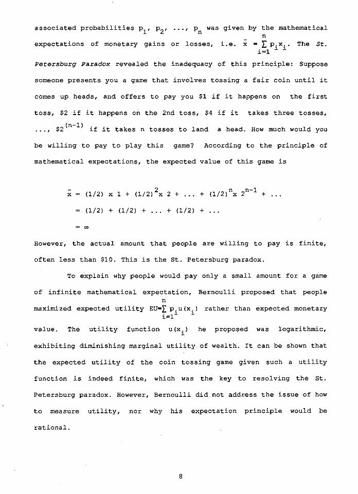
associated probabilities p P2r . . . I P, was given by the mathematical n - .-
expectations of monetary gains or losses, i.e. X = C pixi. The St. i=l
Petersburg Paradox revealed the inadequacy of this principle: Suppose
someone presents you a game that involves tossing a fair coin until it
comes up heads, and offers to pay you $1 if it happens on the first
toss, $2 if it happens on the 2nd toss, $4 if it takes three tosses,
..., $2 (n-l) if it takes n tosses to land a head. How much would you
be willing to pay to play this game? According to the principle of
mathematical expectations, the expected value of this game is
However, the actual amount that people are willing to pay is finite,
often less than $10. This is the St. Petersburg paradox.
To explain why people would pay only a small amount for a game
of infinite mathematical expectation, Bernoulli proposed that people n
maximized expected utility E U = ~ p.u(x.) 1 1 rather than expected monetary i=l
value. The utility function U (xi) he proposed was logarithmic,
exhibiting diminishing marginal utility of wealth. It can be shown that
the expected utility of the coin tossing game given such a utility
function is indeed finite, which was the key to resolving the St.
Petersburg paradox. However, Bernoulli did not address the issue of how
to measure utility, nor why his expectation principle would be
rational.

I t was no t u n t i l John Von Neumann and Oskar Morgenstern (1944)
t h a t expected u t i l i t y maximization was formal ly proved t o be a r a t i o n a l
4 d e c i s i o n c r i t e r i o n . Using f i v e q u i t e reasonable p o s t u l a t e s , they
showed t h e e x i s t e n c e of a u t i l i t y index, U ( . ) , such t h a t t h e expec ted n
u t i l i t y of a r i s k y prospec t , E U = ~ piu(xi) , r e p r e s e n t s t h e i n d i v i d u a l r s =l
p re fe rence o r d e r i n g over r i s k y prospec ts , (plr . . . p ,; xl, ..., xn) .
Thi s i s t h e famous expected u t i l i t y t heo ry t h a t has p l ayed a l e a d i n g
r o l e i n t h e o r i e s of choice under u n c e r t a i n t y t o d a t e . Given i t s
normative appea l and s i m p l i c i t y , t h e EU theory has been used i n many
a p p l i c a t i o n s i n t h e economics of unce r t a in ty s i n c e t h e second world
war.
While most r e s e a r c h e r s a t f i r s t accepted VNMrs theory , A l l a i s
(1953) ques t ioned t h e independence axiom, which i s one of t h e c r u c i a l
axioms i n EU. By d e v i s i n g counter examples, he showed t h a t t h e EU
t h e o r y i s n o t compat ible w i th t h e p re fe r ence f o r l o t t e r i e s i n t h e
neighborhood of c e r t a i n t y . Th i s has become widely recognized a s t h e
" A l l a i s Paradox".
The A l l a i s paradox invo lves t h e fo l lowing two ques t i ons :
1) Do you p r e f e r s i t u a t i o n A t o s i t u a t i o n B?
S i t u a t i o n A:
- c e r t a i n t y of r ece iv ing $1 m i l l i o n
S i t u a t i o n B:
4 T h o u g h a x i o m a t i c e x p e c t e d u t i l i t y theory had . b e e n developed e a r l i e r by
Ramsey (1931), t h e account of it g iven i n t h e 'Theory o f Games and
Economic Behavior' by Von Neumann and Morgenstern is what made i t
m u c a t c h on".

- a 10% chance of winning $5 million
an 89% chance of winning $1 million
and a 1% chance of winning nothing
( 2 ) Do you prefer situation C to situation D?
Situation C:
- an 11% chance of winning $1 million
and 89% chance of winning nothing
Situation D:
- a 10% chance of winning $5 million
and a 90% chance of winning nothing
It can be shown that, according to the EU theory, an answer of "Aw to
the first question implies an answer of "C" to the second question, and
a choice of "B" in the first question implies a choice of "D" in the
second question. However, after analyzing the answers, Allais found
that 53 percent of subjects chose "A" in the first question and "D" in
the second question, which is clearly inconsistent with EU predictions.
Just as the St. Petersburg paradox led Daniel Bernoulli to
replace the principle of rnaximization of the mathematical expectation
of monetary values by the principle of rnaximization of expected
utilities, the Allais paradox has led researchers to reconsider
the expected utility theory.
Over the last decade, many researchers have developed
generalized expected utility theories in attempt to resolve the Allais
paradox. Unfortunately, unlike the case of the St. Petersburg paradox,

5 t h e A l l a i s paradox has not y e t been resolved s a t i s f a c t o r i l y .
2.2 THE EXPECTED UTILITY MODEL AND ALLAIS PARADOX
Consider t h e following l o t t e r y with th ree f i n a l outcomes: (pl, 3
pZr p3; X X X ) , where 1 p = 1 and x > x > x 1, 2, 3 1 2 3,
(xl i s p r e f e r r e d t o i
i=l
X which i s p re fe r red t o X ) . This l o t t e r y would y i e l d outcome X . with 2 3 1
p r o b a b i l i t y p Given f ixed outcomes, such a l o t t e r y can be i '
represented by a point i n t h e ~arschak-Machina t r i a n g l e { (p1,p3);
6 plZO, p3Z0 and p +p I1 } a s i n Figure 2 .1 . According t o t h e expected
1 3
u t i l i t y theory, t h e expected u t i l i t y of consuming such a l o t t e r y i s
given by
where U ( . ) denotes t h e Von-Neumann Morgenstern u t i l i t y index. The
assumption X >X >X implies t h a t U (xl) >U (X*) >U (x3) . Given t h e u t i l i t y 1 2 3
index, EU has t h e property of l i n e a r i t y i n p r o b a b i l i t i e s . Graphically,
t h e l i n e a r i t y proper ty of t h e EU model can be i l l u s t r a t e d i n terms of
5 As will be discussed in section 2.3, no single alternative theory
could explain all the data generated from experiments conducted in
existing empirical studies.
6 Following the existing literature, we restrict our discussions to the
three-event lotteries. The Marschak-Machina triangle adopted by
Marschak (1950) and popularized by Machina in the 1980's is a very
convenient graphical representation of such a lottery.
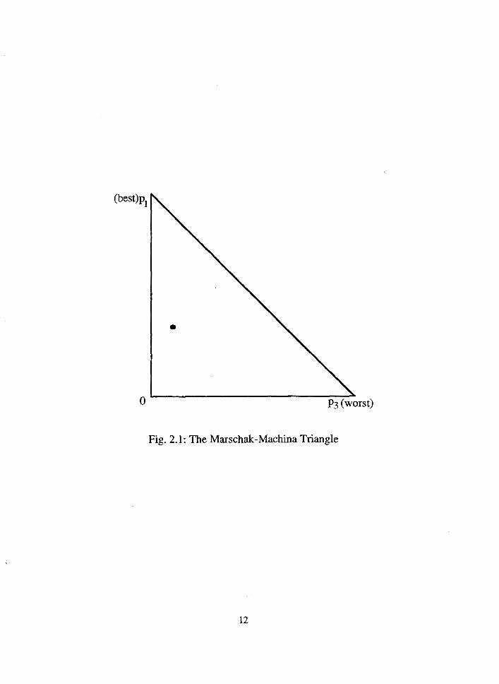
Fig. 2.1 : The Marschak-Machina Triangle

indifference curves in the Marschak-Machina triangle. An indifference
curve of the EU model is a set of probabilities (p p ) with the same 1' 3
expected utility u:
Rewriting equation (2.2) in slope-intercept form,
The indifference curve is a straight line of slope
[U (X*) -U (x3) 1 / [U (xl) -U (x2) 1 . Given the utility index, the slope is
constant. Thus indifference curves are parallel straight lines with
more preferred indifference curves lying to the northwest as in Figure
2.2.1 Allais Paradox and the "Fanning-Out" Effect
The Allais paradox is restated here for the purpose of
illustrating the fanning-out effect. This problem involves choosing one
lottery from each of the following pairs:

where {xl, x2, x3 } ={ $5m, $lm. $01 . These four lotteries form a
parallelogram represented by the broken lines in the (p1, p3) triangle,
as in Figures 2.2a and 2.2b. The parallel straight lines in Figure 2.2a
are EU indifference curves. If these indifference curves are flatter
than the broken lines connecting lotteries A and B, or C and D, EU
implies a choice of B in the first pair and D in the second pair;
similarly if EU indifference curves are steeper than the broken lines,
the choice would be A in the first pair and C in the second pair.
However, many researchers including Allais (1953), Morrison (1967),
Slovic and Tversky (1974), and Kahneman and Tversky (1979) have found
that the modal if not majority of subjects have chosen A in the first
pair and D in the second. According to Machina (1987), this suggests
that indifference curves are not parallel but rather fan out as in
Figure 2.2b.
2 . 2 . 2 Violations of the EU Theory
The Allais paradox exemplifies a class of similar violations of
expected utility theory. The two most well-known violations are the
common consequence effect and the common ratio effect. The Allais
paradox is a common consequence violation.
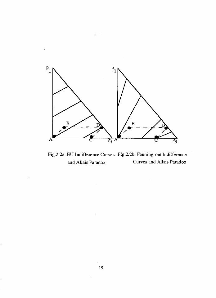
Fig.2.2~ EU Indifference Curves Fig.2.2b: Fanning-out Indifference
and Allais Paradox Curves and All.ais Paradox

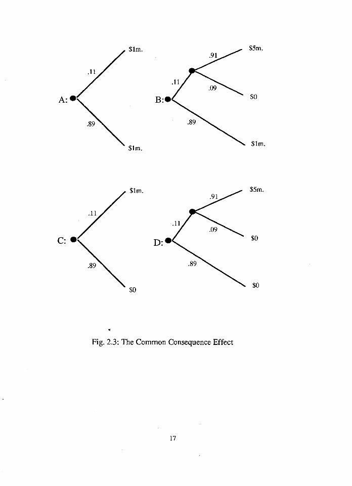
The common consequence e f f e c t can be demonstrated i n A l l a i s t
exper imenta l problem, r e w r i t t e n u s ing t h e compound l o t t e r y s t r u c t u r e s
shown i n F igure 2 . 3 . H e r e each branch r e p r e s e n t s a s u b l o t t e r y .
According t o t h e expected u t i l i t y theory , A i s p r e f e r r e d t o B i f and
on ly i f
Th i s a l s o imp l i e s t h a t C i s p r e f e r r e d t o D. However, a s mentioned i n
t h e p rev ious s e c t i o n , r e sea rche r s have found a tendency f o r s u b j e c t s t o
choose A i n t h e f i r s t p a i r and D i n t h e second p a i r . The d i f f e r e n c e
between t h e f i r s t p a i r (A, B) and t h e second p a i r (C, D ) i s t h a t t h e
s u b l o t t e r i e s i n t h e lower branches of t h e f i r s t p a i r have a "common
consequence" of $1 m, and t h e s u b l o t t e r i e s i n t h e lower branches of t h e
second p a i r have a "common consequence" of $0. EU i m p l i e s t h a t t h e s e
common consequences would be " i r r e l e v a n t " i n choosing between A and B
i n t h e f i r s t p a i r and C and D i n t h e second p a i r . However r e s e a r c h e r s
such a s Kahneman & Tversky (1979) , MacCrimmon (1968) and MacCrimon and
Larsson ( l 9 7 9 ) , and many o t h e r s , have found a tendency f o r s u b j e c t s t o
choose A i n t h e f i r s t p a i r and D i n t h e second p a i r . Given t h a t t h e
s u b l o t t e r i e s of t h e upper branch a r e t h e same i n bo th p a i r s , such a
swing i n p re fe r ence from more r i s k y t o less r i s k y s u b l o t t e r i e s i n one
branch o f a compound l o t t e r y a s t h e s u b l o t t e r y i n t h e o t h e r branch
C
Fig. 2.3: The Common Consequence Effect

improves ( i n t h e sense of s t o c h a s t i c dominance) i s genera l ly known a s
t h e "common consequence e f f e c t " . I n t u i t i v e l y speaking, a s we move from
t h e lower-right corner of the MarschaK - Machina t r i a n g l e t o t h e upper
l e f t corner, people p r e f e r not t o bear f u r t h e r r i s k i n t h e worst event ,
and p r e f e r t h e l e s s r i s k y l o t t e r y .
Another c l a s s of systematic v i o l a t i o n i s c a l l e d t h e "common
r a t i o " e f f e c t . It can be i l l u s t r a t e d i n Figure 2.4. In Figure 2.4, p>q,
0 < X < y and 0 < r < 1. The t e r m common ratio der ives from t h e
e q u a l i t y of prob (X) /prob (y) i n the f i r s t p a i r and i n t h e second p a i r ,
which i s p/q. Given t h e expected u t i l i t y hypothesis, a r a t i o n a l
individual should choose e i t h e r L i n t h e f i r s t p a i r and L i n t h e 1 3
second pa i r , o r L i n t h e f i r s t p a i r and L i n t h e second p a i r . However 2 4
researchers have found from experiments t h a t t h e modal response i s
incons i s t en t with t h i s EU predic t ion . The fol lowing i s an example
i n i t i a l l y proposed by A l l a i s (1953) and l a t e r used by Kahneman and
Tversky (1979) t o demonstrate t h e common r a t i o e f f e c t . I n t h i s example,
y=$4000, x=$3000, p=1.0, q=0.8, and r=0.25, a s shown i n t h e parenthes is
of Figure 2.4. The "common r a t i o " here i s 1.0/0.8=1.25.
P a i r 1: Choose between
L1 (0,1,0; $400, $3000, 0 )
and
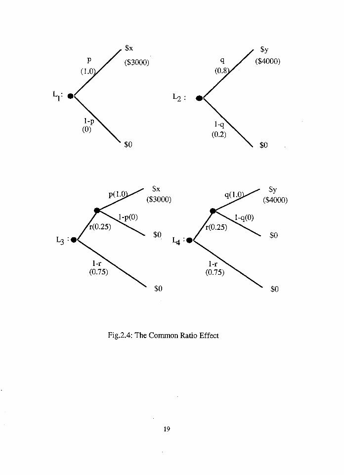
Fig.2.4: The Common Ratio Effect

Pair 2: Choose between
L3 (0, 0.25, 0.75; $4000, $3000, 0)
and
L4 (0.2, 0, 0.8; $4000, $3000, 0)
Kahneman and Tversky presented the gamble pairs to 95
respondents and found that that 80% of the subjects preferred L in the 1
first pair and only 65% of the subjects preferred L in the second 3
pair. Given that EU predicts either a choice of L and L or a choice 1 3
of L* and Lq, the results show the common ratio effect. It can also
be shown, as in Figure 2.5, this effect is consistent with fanning-out
indifference curves.
In summary, a wide range of experimental violations of the EU
theory have been observed. Most of them, if not all, can be interpreted
7 by the fanning-out hypothesis. Thus this hypothesis has been
considered an important key in developing a generalized expected
utility framework to explain violations of the EU model.
7 A s u m m a r y o f t h e l i t e r a t u r e is given by Machina (1982). Attention
here was confined to experimental findings that have had an important
impact on the development of generalized theories of choice under
uncertainty.
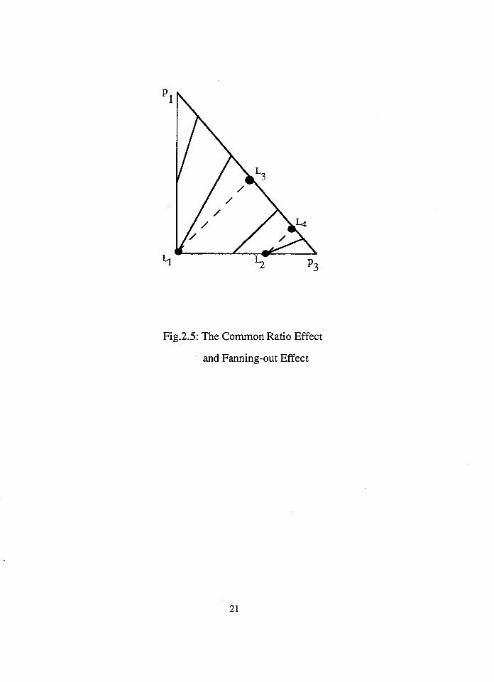
Fig.2.5: The Common Ratio Effect
and Fanning-out Effect
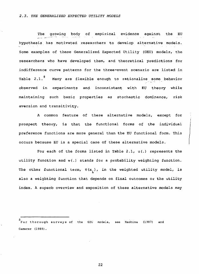
2.3. THE GENERALIZED EXPECTED U T I L I T Y MODELS
The growing body of empirical evidence against the EU ---- - -
hypothesis has motivated researchers to develop alternative models.
Some examples of these Generalized Expected Utility (GEU) models, the
researchers who have developed them, and theoretical predictions for
indifference curve patterns for the three-event scenario are listed in
8 Table 2.1. Many are flexible enough to rationalize some behavior
-
observed in experiments and inconsistent with EU theory while
maintaining such basic properties as stochastic dominance, risk
aversion and transitivity.
A common feature of these alternative models, except for
prospect theory, is that the functional forms of the individual
preference functions are more general than the EU functional form. This
occurs because EU is a special case of these alternative models.
For each of the forms listed in Table 2.1, U(.) represents the
utility function and W ( . ) stands for a probability weighting function.
The other functional term, t(xi), in the weighted utility model, is
also a weighting function that depends on final outcomes or the utility
index. A superb overview and exposition of these alternative models may
8 F o r thorough surveys of the GEU models, see Machina (1987) and
Camerer (1989).

Table 2.1: Examples of the Alternative Models to EU
Prospect Theory
Subjected Weighted Utility
Weighted Utility
Rank-dependent Utility
Kahneman & Tversky (1979)
Karmarkar (1978,1979)
The Fanning Out Hypothesis
Chew & Maccrimmon (1979)
Quiggin (1982)
Implicit Expected Utility Chew (1985) Dekel (1986)
n C Pi u(xi, U*) i=l

be found in .Camerer (1982L. In chapter five, we provide detailed -,~----- - ,-
descriptions of the theories of interest here. What follows is a
brief description of each theory listed in this Table.
The prospect theory of Kahneman and Tversky (1979) is the only
alternative model that does not generalize EU. It differs from EU in
the following ways: first, all outcomes in the prospect theory are
framed as changes from a reference point; second, prospects (i.e.,
lotteries) are edited to make them simpler to evaluate (e.g. outcomes
and probabilities are rounded off or lumped together) ; and third, the
expected utility over an edited prospect is given by a weighted
probability formula as presented in Table 2.1. Kahneman and Tversky
suggest that the weight function, w(p), is increasing in p, subadditive
(W (p) +W (l-p) <l) , and discontinuous at the endpoints 0 and 1. They also
hypothesize that the utility function u(x) is asymmetrical for gains
(x>O) and losses (x<O) . Specifically, U (X) is concave for gains and
convex for losses. This theory is difficult to test because it has many
more degrees of freedom, especially in the editing stage, than any
other theory.
The subjective weighted utility theory was proposed by
Karmarkar, 1978 and 1979. According to this model, the expected utility
for a risky prospect (pl, p2, p3; x2, x2,x3), as given in Table 2-11
a a a depends on a weighting function W (p. ) , where W (pi) =pi / (pi+ (l-pi) , and
a a additional parameter regarded by Karmarkar as a measure of- e -- -_------A -
information processing performance,. Low values of a (O<a<l) underweight ---- -- - - - the objective probability p high values (a>l) overweight p and when
i' ir
a=l, this model reduces to the EU model. This model will be further

explained in chapter five.
Weighted utility theory was developed by Chew and MacCrimmon,
1979 (see also Chew, 1983). As can be seen from Table 2.1, the
weighting function, pir (xi) /C p,r (X. ) is somewhat novel in the sense 1 1
that it combines both probabilities and utilities. Depending on the
choice of ~(x,), the indifference curves of the weighted utility model 1
can either fan-out (this corresponds to the light hypothesis of Chew
and MacCrimmon) , as in Table 2.1, or fan-in (the heavy hypothesis) . 1 i
Although the axioms suggest no obvious psychological interpretation to / !
the weighting function, the weights seem to modify probabilities, 1 possibly reflecting mental distortions or misperceptions, to a degree 1
l
that depends on outcomes X . i
Quiggin (1982,1985) was the first to consider a rank-dependent
utility theory (called anticipated utility). This theory uses a
nonlinear probability transformation function that depends on the order
or rank of the outcomes. Certain specifications of the weighting
function could generate nonlinear fanning-out indifference curves as in
Table 2.1. As proved by Quiggin, this theory has strong axiomatic
foundations. It has been used in some important applications (Quiggin,
1992). This theory is also further explained in chapter five.
J In the fanning-out hypothesis, Machina uses the notion of
(first-order) stochastic dominance. For three-outcome gambles, lottery
A: (p1, p2, p3; X X x3) stochastically dominates B: (ql, q2, q3; X 1, 2, 1,
X 2' x3) if P3<q3 1 and pl>ql. Graphically, point A stochastically
dominates B if A lies to the northwest of B in the ~arschak-Machina
triangle. However, Machina .did not propose specific preference

functions, rather he hypothesized that the local utility functions of -c___- - I.. .
.#
stochastically dominant gambles will exhibit more risk aversion (by the
Arrow-Pratt measure) than local utility functions of stochastically
dominated gambles. This hypothesis predicts that indifference curves,
usually nonlinear, will be steeper for gambles to the northwest of the
Marschak-Machina triangle._ -
Finally, the Implicit Expected Utility function (Dekel, 1986)
generalizes the EU model by replacing u(x) by u(x,u*), where U* is the
expected utility, i.e.,
Indifference curves of Implicit EU are straight lines, but their slopes
vary because u(x,u*) varies with U*. Thus this model describes a person
who uses a different utility function, perhaps reflecting different
degrees of risk aversion along each indifference curve.
2.4 TESTING BETWEEN ALTERNATIVE MODELS
Experiments have identified a number of well-known violations
alternative models
ertainty. These alternative models, with quite
different views of the behavioral processes underlying choices under
uncertainty, are often able to explain some violations of EU -, 4-
predictions. The questions is: Are theoretical predictions of these
alternative models consistent with people's actual choice behavior?

Seve ra l r e c e n t empi r i ca l s t u d i e s (Chew and Waller, 1986; Camerer, 1989;
B a t t a l i o , Kagel and J i r anyaku l , 1990; and Marshal l , Richard and Zarkin,
1992) have a t tempted t o answer t h i s q u e s t i o n by des ign ing new
experiments o r new empi r i ca l methods. Of t h e s e e m p i r i c a l s t u d i e s , a l l
bu t one u se experimental ev idence t o test between t h e a l t e r n a t i v e
9 models.
The gene ra l t e n o r of conc lus ions from t h e s e e m p i r i c a l s t u d i e s
confirm v i o l a t i o n s of t h e EU p r e d i c t i o n s , bu t no s i n g l e t heo ry has
emerged a s a s a t i s f a c t o r y a l t e r n a t i v e . I n what fo l lows , w e p rovide on ly \
a b r i e f d e s c r i p t i o n of experiments and t e s t i n g methods of each s tudy
and t h e i r major r e s u l t s .
Chew and Waller (1986) employed a f our -pa i r l o t t e r y s t r u c t u r e ,
c a l l e d t h e HILO l o t t e r y s t r u c t u r e , t o test weighted u t i l i t y theory . The
HILO l o t t e r y s t r u c t u r e i nvo lves cho ices over f o u r p a i r s of l o t t e r i e s .
F igure 2 . 6 shows a t y p i c a l HILO s t r u c t u r e i n which gamble p a i r s (Ai,
B , ) , i=1,2,3,4 a r e p l o t t e d on t h e Marschak-Machina t r i a n g l e . A s can be 1
seen from t h e t r i a n g l e , t h e s e f o u r gamble p a i r s form t h r e e p a r a l l e l
s t r a i g h t l i n e s l a b e l l e d 1, 2, 3, and 4 . Since EU i n d i f f e r e n c e curves of
an i n d i v i d u a l a r e a l s o s t r a i g h t l i n e s , t h e EU t heo ry p r e d i c t s t h a t t h e
i n d i v i d u a l ' s choice over t h e s e f o u r l o t t e r y p a i r s i s e i t h e r A A A A i f 1 2 3 4
t h e s lope of EU i n d i f f e r e n c e curves i s g r e a t e r t han t h e s lope of l i n e
9 Using seat-belt-usage data, Marshall, Richard and Zarkin (1992) test
Machina's fanning out hypothesis and the "light" hypothesis of Chew
and Waller (1986).

Fig. 2.6: HILO Lottery Structure

segments connec t ing l o t t e r i e s A and B = , 2 , 3 , 4 , o r B B B B i i 1 2 3 4
otherwise . Note t h a t p a i r 2 and p a i r 3 form an A l l a i s t y p e of problem.
For t h i s problem, EU p r e d i c t s a choice of e i t h e r A A o r B B To 2 3 2 3 -
e l a b o r a t e , A l l a i s ' l o t t e r y s t r u c t u r e i s used t o test whether
i n d i v i d u a l s behave c o n s i s t e n t l y over two p a i r s of l o t t e r i e s , and
theHILO l o t t e r y s t r u c t u r e tests t h e cons i s t ency over f o u r p a i r s .
Therefore the H I L O l o t t e r y s t r u c t u r e pe rmi t s s t r o n g e r empi r i ca l tests
10 t han t h o s e i n t h e A l l a i s l o t t e r y s t r u c t u r e . With every H I L O l o t t e r y
s t r u c t u r e , t h e r e a r e 1 6 p o s s i b l e choice p a t t e r n s . Based on observed
f r equenc i e s of choice p a t t e r n s impl ied by a p a r t i c u l a r theory , one can
then test i f t h e t heo ry p r e d i c t s t h e s u b j e c t s ' cho ices b e t t e r t h a n a
chance p r e d i c t i o n model. Using two H I L O l o t t e r y s t r u c t u r e s , Chew and
Waller tested t h e expected u t i l i t y hypo thes i s ( t h e "neu t r a l "
hypo thes i s ) , t h e fanning-out hypothes i s ( t h e " l i g h t " hypo thes i s ) , and
t h e fanning-in hypothes i s ( t h e "heavy" hypo thes i s ) of weighted u t i l i t y
theory . The r e s u l t s i n d i c a t e t h a t t h e " l i g h t " hypothes i s wi th l i n e a r
fanning-out i n d i f f e r e n c e curves i s suppor ted by t h e i r d a t a , t h a t is, it
p r e d i c t s s i g n i f i c a n t l y b e t t e r t han a pure chance p r e d i c t i o n model.
Camerer (1989) a l s o conducted an exper imenta l t es t of s e v e r a l
g e n e r a l i z e d expec ted u t i l i t y t h e o r i e s u s ing an a n a l y s i s of i n d i f f e r e n c e
curves drawn i n t h e Marschak-Machina t r i a n g l e . The t h e o r i e s e v a l u a t e d
w e r e weighted u t i l i t y theory , i m p l i c i t expec ted u t i l i t y theory , t h e
fanning-out hypothes i s , rank-dependent expec ted u t i l i t y .
''The HILO lottery structure i s discussed in more detail in Chapter
three.

Using responses from 14 gamble pairs with each one involving
more risky and less risky gambles of the Allais type, Camerer depicted
an approximate indifference curve pattern based on percentages of
subjects who chose the less risky gambles over the more risky ones in a
Marschak-Machina diagram. He compared these approximate indifference
curves with theoretical predictions of each theory, and concluded that
(Camerer, P82)
"No theory can explain all the data, but prospect theory and 1
the hypothesis that indifference curves fan out can explain l, I
most of them."
Just when the fanning-out hypothesis appeared to be the
solution to Allais paradox, Battalio, Kagel and Jiranyakul (BKJ, 1990)
found evidence of fanning-in rather than fanning-out. Battalio et a1
designed four series of binary choice questions of the Allais type,
involving both losses and gains. Each question required subjects to
indicate which of two gambles they preferred. Based on the frequencies .,.
of choice patterns generated from the subjects, and theoretical
predictions of including Rank-dependent expected - - utility theory (RDEU), Prospect theory and Machina's generalized
expected utility model, they concluded that no single model
consistently explaims,. choices. Among the more important /
. -& J
inconsistencies, they identified conditions generating systematic
/ fanning-in instead of fanning-out of indifference curves in the .
Marschak-Machina triangle.
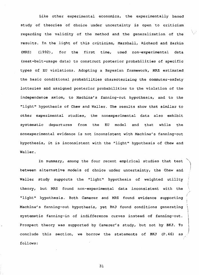
Like other experimental economics, the experimentally based
study of theories of choice under uncertainty is open to criticism \
regarding the validity of the method and the generalization of the
results. In the light of this criticism, Marshall, Richard and Zarkin
(MRZ) (1992), for the first time, used non-experimental data
(seat-belt-usage data) to construct posterior probabilities of specific
types of EU violations. Adopting a Bayesian framework, MRZ estimated
the basic conditional probabilities characterizing the commuter-safety
lotteries and assigned posterior probabilities to the violation of the
independence axiom, to Machinafs fanning-out hypothesis, and to the
"light" hypothesis of Chew and Waller. The results show that similar to
other experimental studies, the nonexperimental data also exhibit
systematic departures from the EU model and that while the
nonexperimental evidence is not inconsistent with Machinafs fanning-out
hypothesis, it is inconsistent with the "light" hypothesis of Chew and
Waller.
In summary, among the four recent empirical studies that test \\ between alternative models of choice under uncertainty, the Chew and
i
Waller study supports the "light" hypothesis of weighted utility
theory, but MRZ found non-experimental data inconsistent with the ' /
"light" hypothesis. Both Camerer and MRZ found evidence supporting
l Machinaf S f anning-out hypothesis, yet BKJ found conditions generating l,,
i systematic fanning-in of indifference curves instead of fanning-out. i Prospect theory was supported by Camerer's study, but not by BKJ. To \
i i
conclude this section, we borrow the statements of BKJ (P.46) as
follows :

"Our overall conclusion is that none of the alternatives to 1
expected utility theory considered here consistently organize the data,
so we have a long way to go before having a complete descriptive model t l of choice under uncertainty." -1
Other independent studies (Harless, 1987; Starmer and Sugden,
1987a, 1987b) also seem to share this view.
2.5 A CRITIQUE ON EXISTING EMPIRICAL METHODS
More than two decades after Allais first challenged expected
utility theory by using experimental evidence, a number of alternative
models were proposed to improve the descriptive ability over the EU
model. Yet existing empirical studies have not found one single theory
that could explain all data. This raises questions about testing
methodology and the validity of the empirical techniques used in the
literature to test theories of choice under uncertainty.
As mentioned in the previous section, a common method used to
test the adequacy of such models typically, the Allais type, is to
compare the frequency of each choice pattern generated from the
experiments with the theoretical predictions of each model. If the
modal response is inconsistent with the theory, then the theory is
considered to be inadequate. Typically, effort is devoted to create a
new generalized expected utility model to explain the modal response.
To see what is involved in this approach, let us take one
experiment from BKJ (1990) for example. Table 2.2 reproduces Table 8
for experiment set 1.1 in their paper (p. 43) . As shown in Figure 2.7,

Fig. 2.7: An Experiment from BKJ

given this experiment, there are four possible choice patterns that
could be generated from a sample population. Column 1 of Table 2.2
lists these choice patterns. The hypothesis that predicts each choice
pattern and choice frequencies are reported in columns 2 and 3
respectively.
Table 2.2 shows that 44.5% (i.e., 16.7%+27.8%) of the subjects
made choices consistent with EU theory, 11.1% of the responses is
consistent with fanning-out hypothesis and 44.4% of the choices is
consistent with fanning-in hypothesis. It is suggested from this result
that since expected utility theory organizes less than half the data
(44.5%), it is considered inadequate. Moreover, with fanning-out
comprising only 20% and fanning-in 80% of the deviations from expected
utility theory, the validity of fanning-out falls dramatically in this
data set. In contrast, the fanning-in hypothesis may be a better
alternative model with EU as a special case.
As another example, let us focus on a more complicated version
of this approach adopted by Chew and Waller (1986). The following set
11 of lotteries is picked from their study.
A1: (0,1,0; $100, $40,$0) B1: (0.5,0,0.5; $100,$40, $0)
A*: (0,1,0; $100, $40, $0) B2
: (O.05,O. 9,O. OS; $lOO,$4O, $0)
A3: (0,0.1,0.9; $100, $40, $0) B3: (0.05,0,0.95; $100, $40, $0)
A4 : (0.9,0.1,0; $100, $40, $0) B4: (0.95,0,0.05; $100,$40,$0)
11 T h i s s e t o f l o t t e r i e s c o r r e s p o n d s t o experiment 1: c o n t e x t la o f Chew
and Waller, 1986.
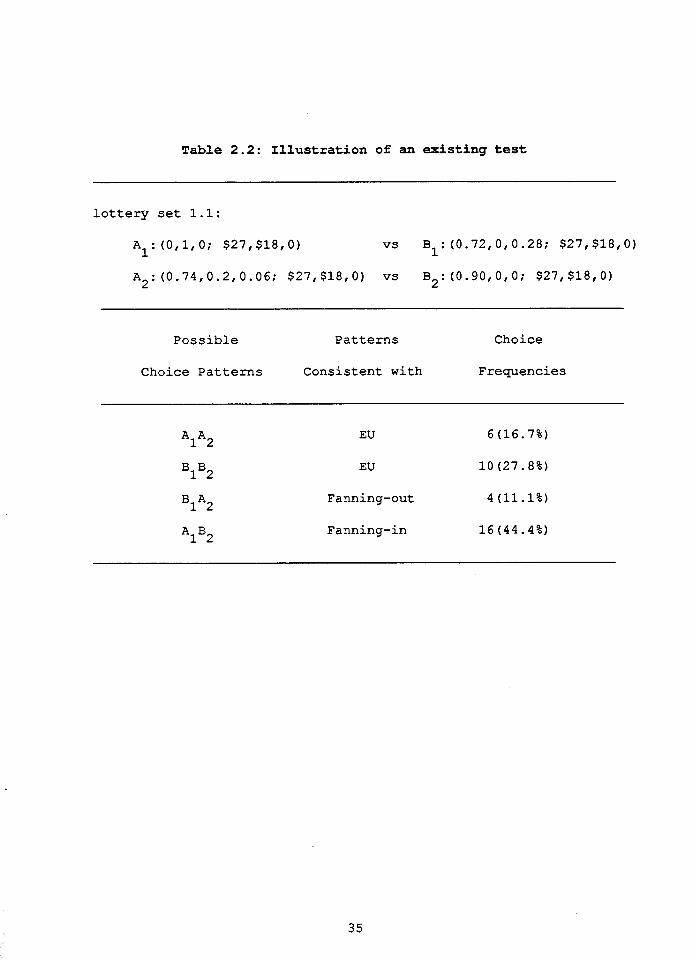
Table 2.2: Illustration of an existing test
lottery set 1.1:
Possible Patterns Choice
Choice Patterns Consistent with Frequencies

These lotteries are also shown in Figure 2.8. From this figure, EU with
parallel indifference curves predicts choice patterns: A A A A and 1 2 3 4
B B B B the fanning-out hypothesis predicts additional choice 1 2 3 4 '
patterns: A A B A and B B B A . and the fanning-in hypothesis predicts 1 2 3 4 1 2 3 4 '
additional choice patterns A A A B and B B A B . Table 2.3 reproduces 1 2 3 4 1 2 3 4
their results generated from 56 subjects. Column 1 contains all
possible choice patterns, column 2 lists the suitable hypotheses and
column 3 reports the observed frequencies. To test weighted utility
theory, Chew and Waller used the observed choice frequencies to
determine whether the EU hypothesis, the fanning-out, or fanning-in
hypotheses predicted the subjects' choice pattern better than a chance
prediction model. In particular, referring to Table 2.3, two of the 16
choice patterns are consistent with the EU hypothesis, therefore, for
this hypothesis to predict better than a chance prediction
node1,the relative frequency of correct predictions would have to be
significantly greater than the chance hit rate of 1/8, or 12.5%.
Furthermore, since 4 of the 16 patterns are consistent with the
fanning-out (or fanning-in) hypothesis, for these hypotheses to predict
better than a chance prediction model, the relative frequencies of
correct predictions would have to be significantly greater than the
chance hit rate of 1/4, or 25%. As shown in Table 2.3, 23% (i.e., 7% +
16%) of responses are consistent with EU; 32% (7% + 16% + 4% + 5%) are
consistent with fanning-in; and 53% (7% + 16% + 5% + 25%) of choices is
consistent with fanning-out. Therefore from these numbers, the EU and
the fanning-out hypothesis predicted significantly better than chance.

A3 P3 (worst)
Fig.2.8: An Experiment from Chew & Waller

Table 2.3: Possible Choice Patterns, Implications of
Weighted Utility and Obsemed Frequencies
Possible Choice Weighted Utility Observed
Patterns Choice Frequencies
A1A2A3A4
A A A B 1 2 3 4
A1A2B3A4
A1A2B3B4
A B A A 1 2 3 4
A1B2A3B4
A1B2B3A4
A B B B 1 2 3 4
B1A2A3A4
B1A2A3B4
B1A2B3A4
B1A2B3B4
B1B2A3A4
B1B2A3B4
B B B A 1 2 3 4
B1B2B3B4
EU, FO, F1
F I
F0
No
No
No
No
NO
No
No
No
No
No
F I
F0
EU, FO, F1
*EU, FO, F1 indicate that the choice pattern is consistent with Expected Utility theory, the Fanning-out and Fanning-in hypotheses, respectively.

Moreover, by comparing t h e t h r e e hypotheses i n terms of p red ic t ive
a b i l i t y (i.e.,number of choices cons i s t en t with each hypothes is ) , Chew
and Waller concluded t h a t t h e fanning-out hypothesis performs t h e bes t
i n expla in ing t h e i r da ta .
A couple of problems a r e apparent from such approaches. F i r s t , h
r e s u l t s from t h e s e s t u d i e s ( i n f a c t from a l l s t u d i e s ) c l e a r l y showed
v a r i a t i o n s of choice p a t t e r n s from a sample population, but t h e
e x i s t i n g t e s t s focus on only t h e modal response. The c r i t e r i o n t h a t
determines whether a p a r t i c u l a r theory is appropr ia te s e e m s t o depend
on whether t h e modal response i s consis tent with t h e theory. This
c l e a r l y ignores t h e p o s s i b i l i t y t h a t d i f f e r e n t people make d i f f e r e n t
choices due t o t a s t e v a r i a t i o n s . Surely, from each da ta s e t , t h e r e a r e , '
always choices incons i s t en t with a l l t heor ie s . Hence, a s a matter of
logic , a l l theory should be r e j e c t e d by such choices. Therefore, any
attempt t o f i n d a theory t h a t explains a l l choices i s doomed t o
f a i l u r e . Secondly, t h e s e tests a r e r a the r ad hoc and unsystematic,
s ince no systematic s t a t i s t i c a l t e s t was cons t ructed t o test t h e
adequacy of t h e o r i e s of choice under uncer ta in ty a t t h e aggregate
l e v e l .
I n t h e l i g h t of t h e s e c r i t i c i sms , a new approach i s developed
here t o t e s t i n g t h e o d e s of choice under uncer ta in ty . This approach i s
based on one important point , t h a t is , t o understand t h e data , one
needs heterogeneity of preferences . I n p a r t i c u l a r , it i s assumed t h a t
ind iv idua l s have d i v e r s e t a s t e s , and t h a t t h e r e e x i s t s a p robab i l i ty
dens i ty funct ion which desc r ibes t h e d iverse t a s t e s across individuals .
Given d a t a generated from labora to ry experiments on choices over gamble

pairs, the density function is estimated through maximum likelihood
estimation techniques. A likelihood ratio test based on the recovered
density function is constructed to evaluate a particular theory of
choice. The next chapter describes the data. Chapter four explains the
new empirical approach.

Chapter Three
THE EXPERIMENTAL DATA
Empirical studies on testing theories of choice under
uncertainty found to date have been based on experimental evidence,
with the exception of Marshall, Richard and Zarkin (1992). In general,
there is an inherent trade-off between experimental and nonexperimental
data. Laboratory experiments offer a high degree of control over the
sampling environment, but the validity of the approach and the
generalization to "real-world1' phenomena is perhaps questionable. On
the other hand, nonexperimental data is more convincing, but sampling
controls are typically poor. Given that the primary purpose of this
study is to develop some empirical techniques to calibrate models of
choice under uncertainty, sampling control is important. Thus
experimental data is employed in this study. Section 3.1 explains the
current experimental design and procedure. Section 3.2 presents the
experimental results. A brief analysis of the data using existing
methodologies in literature is provided in section 3.3. Section 3.4
concludes this chapter.
3.1 Experiments
In this study, three experiments were conducted on three
separate groups of subjects at three different times. Two of the
experiments were used for preliminary studies. The other one was used
to generate data to estimate preferences and test theories of choice

under u n c e r t a i n t y . This s e c t i o n exp la in s t h e experiments: l o t t e r i e s ,
s u b j e c t s and exper imenta l de s ign and procedure.
3.1.1 Lotteries
The l o t t e r i e s w e r e genera ted from t h e Marschak-Machina
t r i a n g l e . Each l o t t e r y i nvo lves t h r e e l e v e l s of payof fs : a c o f f e e mug,
a pen and nothing. The c o f f e e mug, which c o s t $5.95, was a good q u a l i t y
mug w i t h a landscape of Simon F ra se r Univers i ty (S.F.U.). The pen, wi th
a p r i c e of $2.15, was a f i n e pen s p e c i a l l y made wi th an S.F.U. l ogo on
12 it. L o t t e r i e s i nvo lv ing t h e s e p r i z e s can be r ep re sen t ed by d i f f e r e n t
p o i n t s on t h e Marschak-Machina t r i a n g l e . Mugs, pens and no th ing w e r e
used a s p r i z e s t o avoid t h e p o s s i b i l i t y of l o c a l r i s k - n e u t r a l i t y
r e s u l t s . According t o t h e l i t e r a t u r e , such r e s u l t s u s u a l l y a r i s e i n a
cho ice between sma l l money gambles when s u b j e c t s make cho ices based on
expec t ed va lues of t h e l o t t e r i e s r a t h e r t h a n expec ted u t i l i t i e s . I f
s t u d e n t s w e r e g iven d o l l a r p r i z e s , and thought t h a t t h e r e is a c o r r e c t
cho ice i n each s i t u a t i o n , t h e y might be tempted t o choose t h e l o t t e r y
o f f e r i n g t h e h i g h e s t expec ted payoff . Though p re l imina ry experiments
d i d no t s i g n i f i c a n t l y show such r e s u l t s , w e chose t o u se non-monetary
p r i z e s : a mug, a pen, and noth ing a s a precaut ion .
3.1.2 Subjects
Sub jec t s w e r e undergraduate economics s t u d e n t s a t Simon F r a s e r
12 T h e m o n e t a r y v a l u e s o f these ,prizes were not known to the subjects at
the time of experiments.

University. These students were either taking a principles of economics
course or an intermediate economics course. Most of them were not
familiar with the decision theory, and they had not been exposed to
this type of experiment before. Some subjects were given a Crunchie
chocolate bar for participating in the experiments. Some were given a
chance, on a random selection basis, to actually play the lottery they
picked from an experiment. A poll showed 99% of the subjects from one
class claimed to have given serious responses in these experiments.
3.1.3 Experimental Design and Procedure
The experiments were conducted in two stages: a preliminary
stage and a final stage. The purpose of the preliminary experiments was
to gain experience in designing a more efficient and more careful
experiment, that is, to generate more accurate responses for our study,
and to use the data to establish appropriate empirical techniques to
calibrate theories of choice under uncertainty. In this stage, we
designed six sets of lotteries involving both monetary payoffs ($5, $2,
$0) and non-monetary payoffs. Each set contains three lotteries
generated from the Marschak-Machina triangle. The monetary payoffs were
used primarily to examine the local risk-neutrality results as
discussed in the literature (e.g., Quiggin, 1992) . The experimental results from five different undergraduate economics classes, showed no
significant difference between using money and non-money payoffs. The
preliminary study also showed that the initial experimental design was
limited in a number of ways: first, there was not sufficient data
generated for estimation and testing; second, it was difficult to make

any direct comparisons between our experiments and others since other
empirical studies in the literature all used binary choices data, and
we used choices from three lotteries; finally, the design was not
systematic in the sense that the lotteries were generated from the
Marschak-Machina triangle in a somewhat arbitrary fashion.
In the light of these preliminary studies, we designed another
set of experiments to generated the data for estimating and testing the
models of choice under uncertainty. In this experiment, only
non-monetary payoffs were used. Subjects were 284 undergraduate
economics students, who were taking a principles of economics course.
They were asked to respond to 13 binary choice situations. The binary
choices are described in Table 3.1 in which column 1 lists the pair
numbers; column 2 will be explained later. For each pair, columns 3 and
4 describe lotteries A and B respectively, where pl, pZ, and p are the 3
probabilities of winning a coffee mug, a pen and nothing. For example,
pair 13 involves a choice between a 100% chance of winning a coffee mug
(lottery A) and a 100% chance of winning a pen (lottery B). This
lottery pair was designed to divide the sample into two parts: one in
which subjects prefer the mug to the pen and the other one contains
subjects who prefer the pen to the mug. Though both may be used to
recover preferences, they should be used as separate experiments, since
the assumption that u(x ) > u(x ) > u(x ) is necessary to maintain the 1 2 3
graphical interpretation of EU indifference curves. The results from
this show that 250 out of 284 subjects preferred the coffee mug to the

T a b l e 3 . 1 . L o t t e r y P a i r s P r e s e n t e d t o S u b j e c t s
* Lottery A Lottery B
Pair No. Situation (P,, P,, P,) (Pl, P,, P,)
*Prizes: X = a coffee mug, X = a pen, and X = nothing 1 2 3

I J pen. W e w i l l u s e on ly t h i s sample because of t h e l a r g e r sample s i z e .
The o t h e r 12 p a i r s of l o t t e r i e s w e r e designed accord ing t o Chew
and W a l l e r r s H I L O l o t t e r y s t r u c t u r e . A s d i s cus sed i n Sec t ion 2 . 4 of
Chapter 2, t h e HILO l o t t e r y s t r u c t u r e i s a s t r a i g h t f o r w a r d
g e n e r a l i z a t i o n of t h e A l l a i s l o t t e r y s t r u c t u r e . The s t r u c t u r e i s
s p e c i f i e d by two p r o b a b i l i t i e s , a and 6, and t h r e e outcomes, X X H' I'
X where X >xI>xL (H-high outcome, I- in t e rmed ia t e outcome, L-low L, H
outcomes) . These parameters a r e combined i n t o f o u r b i n a r y cho ice
s i t u a t i o n s ( r e f e r r e d t o a s t h e 0, I, L, and H s i t u a t i o n s ) . I n t h e
0 - s i t u a t i o n , A o f f e r s a 1 .00 chance of winning X whi le B o f f e r s a /3 0 I ' 0
chance of winning X and (1-6) chance of winning X . I n t h e o t h e r L H
s i t u a t i o n s , A ( i=I ,L,H) i s ob ta ined by c o n s t r u c t i n g a l o t t e r y w i t h an
a chance of y i e l d i n g A and a l-a chance of y i e l d i n g t h e i outcome
14 I L, H ) , a s shown i n Table 3.2. B I L i s ob ta ined by
0
c o n s t r u c t i n g a l o t t e r y wi th an a chance of y i e l d i n g B and a l-a chance
of y i e l d i n g t h e i outcome (i=I, L, H) . I n t h e c u r r e n t experiment, X = a c o f f e e mug, X = a pen, X =
H I L
noth ing . A s i n d i c a t e d i n column 2 of Table 3.1, Lo t t e ry p a i r s 1 -4 i n
Table 3.1 form HILO s t r u c t u r e 1 i n which a=0.2, 6=0.5; p a i r s 5-8 form
1 3 G i v e n t h a t t h e p u r p o s e h e r e i s t o r e c o v e r p r e f e r e n c e s over l o t t e r y
p a i r s , not t h e f i n a l outcomes of l o t t e r i e s , t h e c u r r e n t t r e a t m e n t of
t h e sample p o p u l a t i o n should not c a u s e any sample s e l e c t i o n b i a s .
14 T h e d e s c r i p t i o n o f t h e H I L O l o t t e r y s t r u c t u r e i s taken from Chew and
Wal le r (1986) . Tab le 3.2 i s b a s i c a l l y t h e same a s Table 1 i n t h e i r
paper .

Table 3 . 2 : The HILO Lo t t e ry S t r u c t u r e
s i t u a t i o n Lot te ry A L o t t e r y B
PxH+ ( l -mxL
a B + (l-a) X 0 I

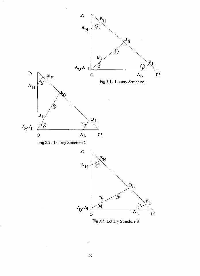
H I L O s t r u c t u r e 2 i n which a=0.25, /3=0.8; and H I L O s t r u c t u r e 3 with
a=0.25, /3=0.2 inc ludes l o t t e r y p a i r s 9-12. These s t r u c t u r e s a r e p l o t t e d
i n Figures 3.1, 3.2, and 3 .3 respect ive ly .
The f i g u r e s show t h a t each s t r u c t u r e has a d i f f e r e n t s lope f o r
t h e l i n e s connecting l o t t e r y Ai and B : 1 f o r s t r u c t u r e 1, 4 f o r i
s t r u c t u r e 2 and 0.25 f o r s t r u c t u r e 3. The numbers t h a t appear above o r
below t h e l i n e segments i n each f i g u r e represent the l o t t e r y p a i r
number corresponding t o d a t a given i n Table 3.1.
A s a l s o i l l u s t r a t e d by these f igures , t h e 12 l o t t e r y p a i r s
cover a l l corners of t h e t r i a n g l e space. The objec t ive i s t o use
l o t t e r i e s from d i f f e r e n t regions of t h e Marschak-Machina t r i a n g l e t o
c a l i b r a t e models of choice under uncer ta in ty .
The experiment proceeded a s follows : F i r s t , t he experimenters
explained t o s tuden t s what t h e experiment was a l l about. A t t h e same
t i m e , sample co f fee mugs and pens were c i r c u l a t e d among s tuden t s t o
f a m i l i a r i z e them with t h e p r i zes . Second, a response sheet with simple
i n s t r u c t i o n s , reproduced i n t h e appendix t o t h i s chapter, was handed
out and explained t o each s tudent . The s tuden t s were asked t o read t h e
i n s t r u c t i o n s f i r s t and then wait f o r t h e experimenter t o expla in t h e
l o t t e r i e s . Third, using an overhead projec tor , t h e experimenter
presented each p a i r of l o t t e r i e s on a separa te t ransparency using t h e
diagram shown ( f o r p a i r 1) i n Figure 3 . 4 . L o t t e r i e s A and B i n each
p a i r a r e represented by two rec tangular a r e a s of u n i t 1. Each
rec tangular a r e a was d iv ided i n t o th ree colored areas, with t h e red
a rea measuring t h e p r o b a b i l i t y of winning a mug, the yellow area
, - A L P3
Fig 3.1: Lottery Structure 1
0 A L
Fig 3.2: Lottery Structure 2
P 1
Fig 3.3: Lottery Structure 3
49

A: (0,l ,O; mug, pen, nothing)
PEN
B: (0.5,0,0.5; mug, pen, nothing)
COFFEE MUG NOTHING
Fig. 3.4: Gamble pair 1 as presented to subjects

measuring t h e p r o b a b i l i t y of winning a pen, and t h e b l u e a r e a measuring
t h e p r o b a b i l i t y of winning nothing. I n t h i s example, l o t t e r y A w i t h
p r o b a b i l i t y (0 ,1 ,0) i s represen ted by t h e r e c t a n g u l a r a r e a e n t i r e l y
co lo red by yellow, and i n d i c a t e s a 100% chance winning a pen. L o t t e r y
B wi th p r o b a b i l i t y (0.5,0,0.5) i s r ep re sen t ed by t h e r e c t a n g u l a r a r e a
co lo red h a l f i n red and ha l f i n b lue . It i n d i c a t e s a 50% chance of
winning a mug and a 50% chance of winning nothing. When p r e s e n t i n g each
p a i r , t h e exper imenter a l s o v e r b a l l y exp la ined t h e l o t t e r i e s . The
s t u d e n t s were asked t o make a choice by c i r c l i n g e i t h e r A o r B on t h e
15 response s h e e t a f t e r each p a i r was presen ted . F ina l ly , a f t e r
complet ing a l l 13 p a i r s , t h e exper imenters c o l l e c t e d response s h e e t s
and rewarded each s t u d e n t with a c runchie choco la t e b a r . The experiment
took approximately 30 minutes.
3.2 RESULTS
The r e s u l t s a r e r epo r t ed i n two p a r t s . F i r s t , d e s c r i p t i v e d a t a
is p re sen t ed r ega rd ing t h e s u b j e c t s r cho ices . Second, t h e s e cho ices a r e
ana lyzed u s i n g t h e previous empi r i ca l methods adopted i n t h e
l i t e r a t u r e .
Table 3.3 r e p o r t s t h e f requenc ies of A and B, cho ices i n each i 1
15 F o l l o w i n g m a j o r i t y o f t h e researchers, indifference curves between two
lotteries was not allowed in this experiment.

Table 3.3: Frequencies of choices
cho i ce s s t r u c t u r e 1 s t r u c t u r e 2 s t r u c t u r e 3

of t h e t h r e e H I L O s t r u c t u r e s . From t h i s t a b l e , w e can see t h a t t h e
r e s u l t s from t h e 12 p a i r s of l o t t e r i e s d i f f e r from one s t r u c t u r e t o
another . I n l o t t e r y s t r u c t u r e 1, a tendency t o p r e f e r A a l t e r n a t i v e i
ove r B a l t e r n a t i v e ( i=1,2,3,4) was ev ident , except i n t h e i
I - s i t u a t i o n . For l o t t e r y s t r u c t u r e 2, t h e tendency was t o p r e f e r Bi
ove r A ( i=5 ,6 ,7 ,8 ) , except i n t h e H-s i tua t ion . F i n a l l y i n s t r u c t u r e 3, i
t h e m a j o r i t y of s u b j e c t s chose A over B i n a l l H-I-L-0 s i t u a t i o n s i i
9 , 1 , l , 2 . Notice t h a t t h e s lopes of t h e segments connect ing
l o t t e r y p a i r s A and B a r e d i f f e r e n t between H I L O s t r u c t u r e s (1 f o r i i
s t r u c t u r e 1, 4 f o r s t r u c t u r e 2 and 1 / 4 f o r s t r u c t u r e 3 ) a s shown i n
F igu re s 3 .1 , 3.2, and 3.3 r e spec t ive ly . Therefore t h e s e d i s p a r a t e
r e s u l t s may simply r e f l e c t t h e s e s l o p e d i f f e r e n c e s , a s w i l l b e seen i n
t h e fo l lowing a n a l y s i s .
3 .3 DATA ANALYSIS
The d a t a i s f i r s t analyzed u s i n g t h e e x i s t i n g empi r i ca l methods
i n t h e l i t e r a t u r e . The purpose here i s t o o b t a i n some p r i o r in format ion
on whether t h e EU theory i s c o n s i s t e n t wi th ou r d a t a and i f not, what
t heo ry cou ld s e r v e a s a b e t t e r a l t e r n a t i v e . Table 3.4 r e p o r t s t h e
observed f r e q u e n c i e s f o r each H I L O s t r u c t u r e . The modal response was
ABAA i n s t r u c t u r e l ( p a i r s 1 -4) , BBBA i n s t r u c t u r e 2 ( p a i r s 5-81 and
AAAA i n s t r u c t u r e 3 ( p a i r s 9-12). The expected u t i l i t y t heo ry p r e d i c t s
e i t h e r AAAA o r BBBB i n a l l t h r e e s t r u c t u r e s . But t h e pe rcen tages of t h e

T a b l e 3 .4 : P o s s i b l e C h o i c e P a t t e r n s and O b s e r v e d Frequencies
of the HILO structures
P o s s i b l e A l t e r n a t i v e S t r u c t u r e 1 S t r u c t u r e 2 S t r u c t u r e 3
c h o i c e Hypothesis* p a i r s 1 - 4 p a i r s 5-8 p a i r s 9-12
p a r t t e n s
1 AAAA
2 BAAA
3 ABAA
4 BBAA
5 AABA
6 BABA
7 ABBA
8 BBBA
9 AAAB
1 0 BAAB
11 ABAB
12 BBAB
13 AABB
1 4 BABB
1 5 ABBB
1 6 BBBB
ALL
NO
NFO
NO
LFO
NFO
NFO
LFO
F I N
NO
NO
F I N
NO
NO
NO
ALL
ALL indicates all hypotheses listed in this table including EU. NO means that no existing hypothesis could explain the choice. NE'O indicates non-linear fanning-out indifference curves. W O indicates linear fanning-out indifference curves. F I N stands for fanning-in indifference curves.

subjects who made these choices are only 26.4% ( 19.6% + 6.8%) in
structure 1, 14.4% (8.4% + 6%) in structure 2, and 55.2% (53.2% + 2%)
in structure 3. Hence the EU model does not explain almost 74% of
subjects in structure 1, 86% in structure 2 and 45% in structure 3.
Also in Table 3.4, column 2 lists alternative hypothesis of
indifference curve that may be used to explain the choices shown in
column 1. For example, choices AAAA and BBBB, accounted for 26.4%
(19.6% + 6.8%) may be explained by all theories including EU. Figures
3.5 and 3.6 show these choices with EU parallel indifference curves in
the Marschak-Machina triangle. Choices ABAA and ABBA, which accounts
for 38.8% of total population, may be explained by non-linear
fanning-out hypothesis for structure 1 as in Figures 3.7 and 3.8.
To summarize the results from Table 3.4, we make the following
observations: (1) No single hypothesis can organize all the data; (2)
up to 14.4% of choices could not be explained by any theory listed;
(3) the fanning-out hypothesis, including both linear fanning-out (LFO)
and non-linear fanning-out (NFO), seem to explain a large portion of
the data set. The frequencies of the choices implied by this hypothesis
(i.e., choices 1,3,5,6,7,8,16 from Table 3.4) were summing up to 83.2%
for structure 1, 92.4% for structure 2 and 92% for structure 3. These
results suggest that the fanning-out hypothesis may be an attractive
hypothesis for our data. It reflects certain behavioral regularities:
sure gains are much more attractive than uncertain gains with equal
expected value and small chance of a zero payoff.
To further explore the choice patterns, we also adopt an

Fig. 3.5: Choice of AAAA with EU Indifference Curves
Fig. 3.6: Choice of BBBB with EU Indifference Curves

Fig. 3.7: Choice of ABAA with NFO Indifference Curves
Fig. 3.8: Choice of ABBA with NFO Indifference Curves

empirical method used by Camerer (1989). In his study, Camerer proposed
two ways of analyzing the data: between-subjects and within-subjects.
Between-subjects tests look at patterns of averaged choices;
within-subjects tests look at the averaged patterns of choices. Camerer
used between-subject analyses to suggest conclusions that were verified
by within-subjects analyses. This approach is another version of the
representative consumer approach, because between-subject measurements
of average behavior provide a picture of how such a hypothetical
representative agent might act. Figure 3.9 shows the analysis for HILO
structure 1 of our data set. In this figure, the thin lines connect the
two lotteries A and B in each pair. The thick line represents the
fraction of subjects who chose lottery A in the pair (the fraction is
written next to the thick line). For instance, the thin line labelled 4
connects (0.8, 0.2, 0) and (0.9, 0, 0.1) , the two lotteries in pair 4,
85.5% of the subjects chose A over B. The slope of the thick line is a
linear function of this fraction. If all subjects chose lottery A, the
thick line will be perfectly vertical; if all chose lottery B, it will
be horizontal. If half chose A and half chose B, the thick line will
have a slope of one (it will superimpose on the thin line connecting A
and B). Therefore, according to Camerer, the thick lines are analogous
to indifference curves even though they have no formal meaning. The EU
model predicts that these lines will be parallel over the space of the
triangle. But our results show that these lines are becoming steeper as
we move from the lower-right corner to the upper-left corner of the
triangle. In addition, the results from pairs 1 and 2 indicate that the

Fig. 3.9: Observed "Indifference Curve" Pattern

i n d i f f e r e n c e curves may no t even be s t r a i g h t l i n e s i n s i d e t h e t r i a n g l e .
Its s l o p e g e t s b igge r when w e move from t h e o r i g i n t o t h e edge of t h e
t r i a n g l e . The broken l i n e i n F igure 3 .9 d e p i c t s an approximate p a t t e r n
of t h e " ind i f f e r ence curves" . It shows t h a t t h e " i n d i f f e r e n c e cu rvesn
indeed f a n ou t a s w e move from t h e lower- r igh t co rne r t o t h e uppe r - l e f t
co rne r of t h e ~arschak-Machina t r i a n g l e . Furthermore, t h e s e
i n d i f f e r e n c e curves may be non l inea r i n t h e neighborhood of t h e o r i g i n
i n s i d e t h e t r i a n g l e . This provides a good s t a r t i n g p o i n t f o r u s t o
s ea rch f o r a l t e r n a t i v e models of choice under u n c e r t a i n t y , which w i l l
be exp la ined i n Chapter 5.
3.4 CONCLUDING RE:MWWS
This chap te r s o f a r has analyzed cho ices gene ra t ed from
classroom experiments u s ing e x i s t i n g methods. I t was found, l i k e many
o t h e r s t u d i e s , t h a t v i o l a t i o n of t h e EU model was e v i d e n t i n t h i s d a t a
set, and t h a t t h e fanning-out hypothes i s does e x p l a i n a b i g p a r t of t h e
d a t a set . However, t h e d a t a a l s o e x h i b i t s many o t h e r d i f f e r e n t choice
p a t t e r n s . I f w e cont inue t o pursue t h e a n a l y s i s of a r e p r e s e n t a t i v e
consumer, any theo ry w i t h homogeneous p re fe r ences w i l l be d i r e c t l y
r e j e c t e d by ou r da t a , because t h e d a t a shows t h a t t h e r e a r e choice
p a t t e r n s t h a t a r e i n c o n s i s t e n t wi th any theory . This i s t h e key
d e f i c i e n c y w e see wi th e x i s t i n g methods. Furthermore, a s w e have a l s o
seen, t h e prev ious a n a l y s i s i s r a t h e r unsystematic i n t h a t no
s t a t i s t i c a l i n f e r e n c e s w e r e made about t h e hypothes i s . TO use a l l

information to construct a systematic test of theories of choice under
uncertainty, we develop in the following chapter a new approach in
which heterogeneity of preferences among individuals is assumed.

A p p e n d i x To C h a p t e r T h r e e
RESPONSE SHEET PROVIDED TO STUDENTS
I . Introduction
This i s an experiment about l o t t e r i e s . You a r e under no
ob l iga t ion t o p a r t i c i p a t e . The r e s u l t w i l l be used f o r a research
p r o j e c t . Your cooperation would be g r e a t l y appreciated. It i s not a
test of whether you can p ick t h e 'bes t ' l o t t e r y . Which l o t t e r i e s you
p r e f e r is a mat ter of personal t a s t e . P lease make sure t h a t your
choices a r e not a f f e c t e d by o thers by working s i l e n t l y .
11. C h o i c e s
Row Lottery
C h a p t e r F o u r
PREFERENCE RECOVERY FOR THE EXPECTED
UTILITY MODEL
Models of p re fe rence e v a l u a t i o n and demand a n a l y s i s have
t r a d i t i o n a l l y been based on d a t a ob ta ined by d i r e c t observa t ion of
i n d i v i d u a l choice behavior . Such models o f t e n invo lve spec i fy ing a
u t i l i t y s t r u c t u r e f o r a r e p r e s e n t a t i v e consumer. By us ing t h e
a p p r o p r i a t e s t a t i s t i c a l technique, t h e u t i l i t y f u n c t i o n s can be
i n f e r r e d . This t ype of approach f a l l s i n t o t h e ca tegory of e i t h e r
hedonic p r i c e a n a l y s i s ( see , f o r example, Rosen (1974) and Brown and
Rosen (1982)) o r t h e more convent iona l revea led p re fe rence ana lys i s .
Our approach d i f f e r s from t h e s e approaches by assuming t h a t i nd iv idua l
p re fe rences a r e d i v e r s e and t h a t t h e r e e x i s t s a p re fe rence parameter
space i n which llconsumers** a r e l o c a t e d with d i f f e r e n t "addresses" o r
p re fe rence parameters . Aggregate p re fe rences f o r a group of i n d i v i d u a l s
a r e desc r ibed by a p r o b a b i l i t y d e n s i t y func t ion i n t h e space of
p re fe rence parameters . I n t h i s t h e s i s , t h e not ion of preferences
recovery r e f e r s t o t h e e s t ima t ion of such a d e n s i t y func t ion .
This c h a p t e r develops t h e empi r i ca l t echniques used f o r t h e
p re fe rence recovery f o r t h e EU model. I t a l s o c o n s t r u c t s a test on
i n d i v i d u a l choice behavior under t h e EU model. Sec t ion 4 . 1 de sc r ibes
t h e p re fe rences recovery techniques f o r t h e EU model.Section 4.2
r e p o r t s a Monte-Carlo s tudy of t h e e s t ima te s . I n s e c t i o n 4.3, t h e
exper imenta l d a t a p re sen ted i n Chapter 3 is regrouped f o r t h e purpose

of es t imat ing and t e s t i n g t h e EU model. Sect ion 4.4 provides
es t imat ions of the EU model using t h e preference recovery technique
descr ibed above. A test, based on t h e recovered preference dens i ty
funct ion , is const ructed t o test i f t h e EU model adequately expla ins
t h e da ta generated from labora tory experiments. The l a s t sec t ion
summarizes t h e r e s u l t s .
4 . 1 PREFERENCE RECOVERY
Recall equation (2.1) i n Chapter 2, t h e expected u t i l i t y of an
ind iv idua l choosing l o t t e r y (p p2, p3; xl, x2, x3) under t h e EU model
i S
It i s assumed t h a t U (xl) >U (X ) >U ( X ) . Without l o s s of genera l i ty , w e 2 3
assume t h a t U (X )=l, U ( X )=v, U (x3) =O. The consumer's expected u t i l i t y 1 2
of choosing t h e l o t t e r y then becomes
I n t h e case of monetary payoffs, v i s t h e c e r t a i n t y equivalence
parameter. Higher values of v imply t h a t t h e consumer i s more r i s k

16 averse. However, when non-monetary payoff S are used, this
interpretation of the v parameter is not appropriate. In this case, we
shall consider v only as a diversity parameter that distinguishes one
individual from another. Since the choice of any one consumer, given a
set of lotteries, depends on that consumer's value of v, each
consumer's preferences can be completely represented by a single value
of v. Given a sample population, aggregate preferences of consumers can
then be represented by a probability density function •’(v). The
question addressed is how to estimate •’(v) using choices generated from
laboratory experiments.
Different approaches may be used to estimate such a density
function. Examples are nonparametric smoothing techniques and maximum
likelihood estimation techniques. We shall choose the latter in this
thesis because it is a well known and widely accepted technique. To use
the maximum likelihood approach, we need to specify a parametric form
for the aggregate preference density function f (v; A), where A is a set
of unknown parameters to be estimated. The statistical problem
presented is to estimate A using choices from experiments.
To see what is involved in the estimation procedure, consider
the following set of binary choice lotteries:
16 M a c h i n a ( 1 9 8 2 ) p o i n t e d o u t t h a t v / ( l - v ) c a n b e u s e d t o measure r i s k
a v e r s i o n o f a consumer much l i k e t h e Ar row-Pra t t measure. The l a r g e r
i s t h e v v a l u e , t h e more r i s k a v e r s e i s t h e i n d i v i d u a l ( l a r g e r v means
s t e e p e r EU i n d i f f e r e n c e c u r v e s ) .

According t o equa t ion 4 . 1 , t h e expected u t i l i t y of an i n d i v i d u a l
choosing each o f t h e s e l o t t e r i e s i s given by
Note t h a t g iven Equat ion (4 .2 ) , t h e expected u t i l i t y of choosing any
l o t t e r y w i th p r o b a b i l i t y d a t a ( p 1 p2, p ) i s a l i n e a r f u n c t i o n of v . 3
W e s h a l l c a l l t h e s e EU lines. Figure 4 . l a shows t h e EU l i n e s of a l l s i x
l o t t e r i e s l i s t e d above. The 45' degree l i n e l a b e l l e d EU(AI), EU(A2),
EU(A ) r e p r e s e n t s expec ted u t i l i t i e s from l o t t e r i e s A A2, and A f o r 3 1' 3
a l l p o s s i b l e v a l u e s of v . The o t h e r t h r e e h o r i z o n t a l l i n e s l a b e l l e d
EU (B1) , EU (BZ) , EU (B ) r ep re sen t t h e expected u t i l i t i e s f o r l o t t e r i e s 3
B1, B2, and B r e s p e c t i v e l y . Given any p a i r of l o t t e r i e s , EU imp l i e s 3
t h a t t h e i n d i v i d u a l w i l l choose t h e l o t t e r y wi th t h e h ighe r expected
u t i l i t y c a l c u l a t e d by Equation 4.1. Consider l o t t e r y p a i r 1 f o r
i n s t ance ; t h e EU l i n e s f o r A and B i n t e r s e c t a t v=0.5 a s i n F igure 1 1
4 . l a . Under t h e EU model, any i n d i v i d u a l whose v v a l u e i s less than 0.5
would choose B1 over AI; o therwise, B1 w i l l be chosen over A 1 '
Simi l a r ly , l o t t e r y p a i r 2 d i v i d e s t h e v space i n t o two p a r t s (0 , 0.8)
and (0.8, l ) , and p a i r 3 s p l i t s t h e v space i n t o two p a r t s ( 0 , 0 .2) and

Fig. 4.la: An Illustration of EU Choices
Fig. 4.lb: Histogram and Distribution of v

(0.2, 1). Therefore , t h e t h r e e l o t t e r y p a i r s d i v i d e t h e v space i n t o
f o u r i n t e r v a l s : (0, 0 .2 ) , (0 .2 , 0 . 5 ) , (0.5, 0.81, and (0.8, 1). Under
t h e expec ted u t i l i t y theory , an i n d i v i d u a l who has a v va lue i n (0,
0.2) should choose B i n t h e f i r s t p a i r , B2 i n t h e second p a i r and B 1 3
i n t h e t h i r d p a i r . Hence a choice p a t t e r n B B B r e s u l t f o r t h e t h r e e 1 2 3
b ina ry choice l o t t e r i e s . S imi l a r ly , an i n d i v i d u a l wi th v va lue i n s i d e
(0.2, 0.5) shou ld choose B B A an i n d i v i d u a l whose v va lue l ies 1 2 3;
between 0.5 and 0.8 should choose A1B2A3; f i n a l l y , i n t e r v a l (0 .8 , 1)
17 c o n t a i n s a l l t h e i n d i v i d u a l s who should choose A A A
1 2 3 -
I n summary, given t h e above t h r e e p a i r s of l o t t e r i e s , i f t h e
under ly ing t h e o r y (EU) i s t r u e , t h e r e w i l l be f o u r p o s s i b l e choice
p a t t e r n s gene ra t ed from a sample populat ion: B B B B B A 1 2 3' 1 2 3' A1B2A3f
and A1A2A3, each wi th a corresponding subse t of v. For convenience, w e
denote t h e s e cho ice p a t t e r n s by 1,2,3,4. Given t h e number of s u b j e c t s
who choose each of t h e s e choice p a t t e r n s i n a sample popula t ion , a
his togram based on t h e percentage of i n d i v i d u a l s choosing each choice
p a t t e r n can be c o n s t r u c t e d a s i n F igure 4 . l b . The p r o b a b i l i t y d e n s i t y
func t ion f (v;h) drawn over t h e his togram i s t h e d e n s i t y f u n c t i o n t o be
e s t ima ted .
If w e know f (v;A), t h e p r o b a b i l i t y of an i n d i v i d u a l choosing
p a t t e r n 1, 2, 3, 4 can be de r ived from Figure 4 . l b a s fol lows:
17 Any i n d i v i d u a l who l i e s a t t h e boundary o f t h e s e i n t e r v a l s would b e
i n d i f f e r e n t between two l o t t e r i e s . S i n c e t h e exper imenta l d a t a
d i s c u s s e d i n Chapte r 3 d o e s . no t i n c l u d e i n d i v i d u a l s who expressed
i n d i f f e r e n c e , t h i s c a s e i s d i smissed f o r s i m p l i c i t y .
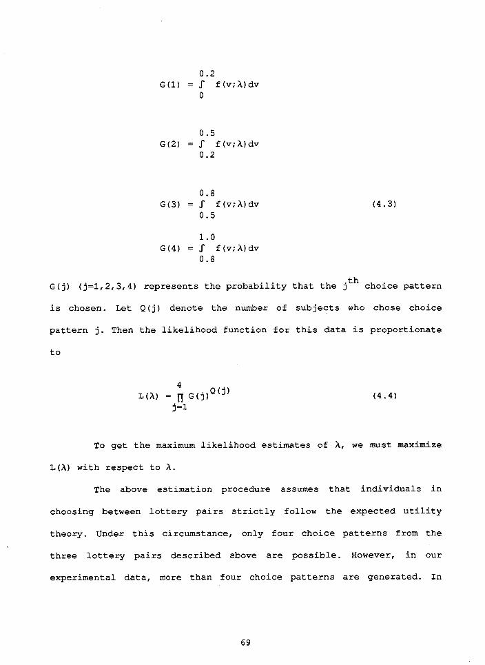
G ( j) (j=l, 2,3,4) represents the probability that the jth choice pattern
is chosen. Let Q(j) denote the number of subjects who chose choice
pattern j. Then the likelihood function for this data is proportionate
To get the maximum likelihood estimates of A, we must maximize
L(A) with respect to h.
The above estimation procedure assumes that individuals in
choosing between lottery pairs strictly follow the expected utility
theory. Under this circumstance, only four choice patterns from the
three lottery pairs described above are possible. However, in our
experimental data, more than four choice patterns are generated. In

fact, for any set of three lottery pairs, there were eight possible
choice patterns: B1B2B3, B1B2A3, A1B2A3, A1A2A3, B1A2A3, B A B 1 2 3'
A1B2B3, A A B which are also indexed by 1, 2, 3, 4, 5, 6, 7, 8 for 1 2 3,
convenience. Therefore given the data, without some elaboration of the
model that permits other choices, one must immediately reject the
model. We elaborate by introducing a trembling hand in the execution of
intended choices. In particular, we make the following assumption:
Individuals in making choices over a lottery pair have trembling hands
18 and sometimes pick the lottery with the lower expected utility. That
is, people simply make mistakes in picking the "correct" lottery. Let 0
be the mistake parameter representing the probability of an individual
choosing the less-preferred lottery. Given the intention to choose
lottery A in preference to lottery B, the individual actually chooses A
with probability 1-0, and B with probability 0. To elaborate further,
suppose that an individual presented with lottery pair A and B has a
higher expected utility for lottery A. Without a trembling hand, the
probability of choosing A is 1.0 and the probability of choosing B is 0
under the EU model. In contrast, with a trembling hand, the
probability of choosing A and B are (1-0) and 6, respectively.
Given the probability of an individual falling in the jth
18 A n a l t e r n a t i v e e l a b o r a t i o n i s to introduce an added error term to
(4.2), which leads to the random utility model or a class of
probabilistic choice models in econometrics literature. However this
error term is often interpreted as 'tomissions" (e.g., unobservables
and model misspecif ication) by researchers (See, for instance,
Anderson, de Palma and Thisse, 1992). In addition, such models with
systematic taste variations across individuals i . e . different v
values) are not identified with aggregate data.

choice i n t e r v a l : G ( j ) , j=1,2,3,4, and t h e mis take parameter 8, t h e
p r o b a b i l i t y of any i n d i v i d u a l choosing each of t h e e i g h t p o s s i b l e
choice p a t t e r n s i s cons t ruc t ed a s fol lows:
To show e x a c t l y how t h e s e R ( j ) S ( j= l , . . . , 8) w e r e obtained,
le t ' s t a k e R ( 1 ) a s an example: R ( 1 ) r e p r e s e n t s t h e p r o b a b i l i t y of any
i n d i v i d u a l choosing choice p a t t e r n 1, o r B B B . From Figure 4 . l a and 1 2 3
Equations (4.3) , t h e p r o b a b i l i t i e s of an i n d i v i d u a l f a l l i n g i n t o each
of t h e f o u r choice i n t e r v a l s a r e given by G ( l ) , G ( 2 ) , G(3) , and G(4 ) .
I f t h e s u b j e c t f a l l s i n t h e f i r s t i n t e r v a l , he r b e s t choice p a t t e r n
would be B1BZB3, b u t with mistake 0, she w i l l execute t h i s choice
3 p a t t e r n wi th p r o b a b i l i t y l - . Therefore, t h e p r o b a b i l i t y of an
i n d i v i d u a l f a l l i n g i n t o i n t e r v a l 1 and choosing choice p a t t e r n 1 i s
3 (1-8) G ( 1 ) ; i f t h e i nd iv idua l f a l l s i n t o t h e second i n t e r v a l , h e r b e s t
choice p a t t e r n would be B B A For h e r t o choose B B B she has t o 1 2 3' 1 2 3'
make no mistakes i n p a i r s 1 and 2 and one mistake i n p a i r 3 . Hence t h e
p r o b a b i l i t y of an i n d i v i d u a l f a l l i n g i n t o t h e second i n t e r v a l and
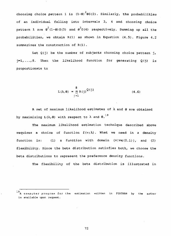
choosing choice pattern 1 is (1-8) 2 8 ~ (2 . Similarly, the probabilities of an individual falling into intervals 3, 4 and choosing choice
2 3 pattern 1 are 8 (1-B)G(3) and 8 G(4) respectively. Summing up all the
probabilities, we obtain R (1) as shown in Equation (4.5) . ~igure 4.2 summarizes the construction of R(1).
Let Q (j) be the number of subjects choosing choice pattern j,
j=1,.,8 Then the likelihood function for generating Q(j) is
proportionate to
A set of maximum likelihood estimates of A and 8 are obtained
19 by maximizing L (A, 8) with respect to h and 8.
The maximum likelihood estimation technique described above
requires a choice of function f (v;A). What we need in a density
function is: (1) a function with domain v v ( 0 . 1 ) and (2)
flexibility. Since the beta distribution satisfies both, we choose the
beta distributions to represent the preference density functions.
The flexibility of the beta distribution is illustrated in
19 A c o m p u t e r p r o g r a m f o r t h e e s t i m a t i o n w r i t t e n i n FORTRAN by t h e au thor
i s a v a i l a b l e upon r e q u e s t .

B 1 B 2 B 3 (interval 1)
B1 B2A3 (interval 2)
A l B 2 A 3 (interval 3)
A 1 A 2 A 3 (interval 4)
Fig. 4.2: Constructing Probability R(1)

Figure 4 . 3 in which the probability density function exhibits a large
degree of variability to the extent that distribution has a single
mode. Such flexibility is needed to recover preferences given little
knowledge about the distribution of v. However, it should be noted that
such flexibility is also limited. For example, the beta distribution
function does not include multi-mode distributions.
The beta probability density function (PDF) is defined as
where /3 ( A l , h 2 ) is the beta function, and
Parameters A and A are the parameters to be estimated ( A >Or 1 2 1
A 2 > 0 ) . putting f (v; All A2) into Equation ( 4 . 3 ) , we obtained the
estimates of A and A2 using numerical methods to maximize Equation 1
(4.6).
The mean and variance of v are given by the following
Equations.
Mean = hl/ (Al+A2)
2 Variance = A A / ( h l + A 2 ) ( A +A +l)
1 2 1 2

Fig. 4.3: The Beta Distribution Functions
Function hl % I
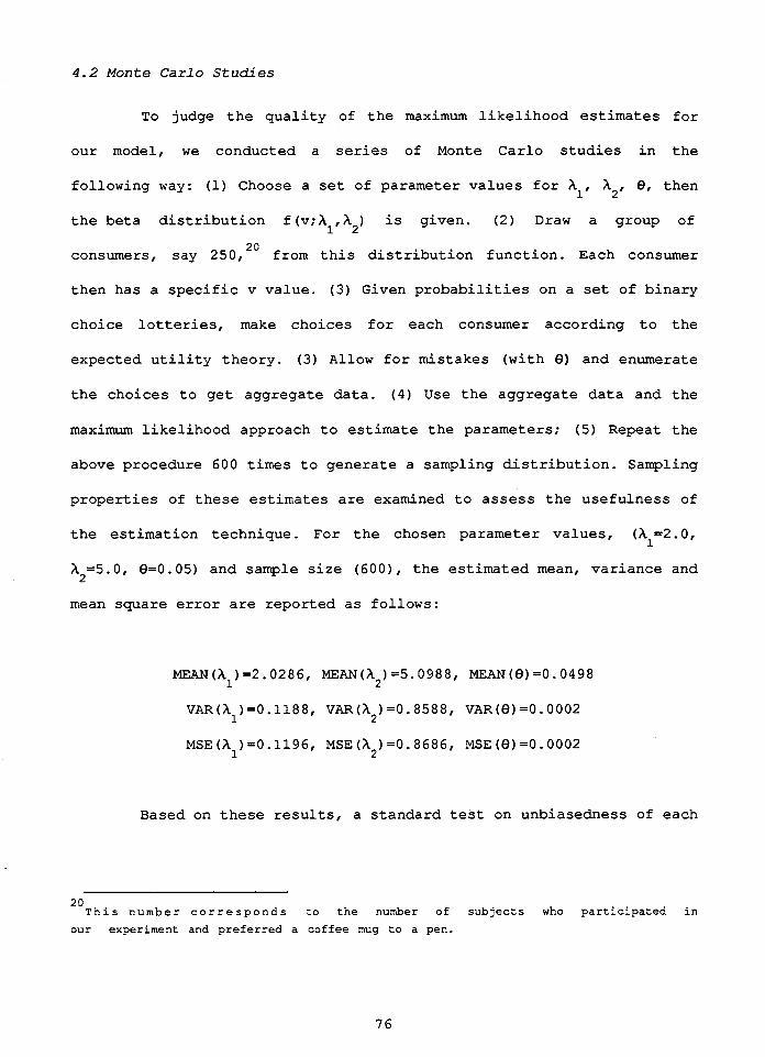
4.2 Monte C a r l o S t u d i e s
To judge the quality of the maximum likelihood estimates for
our model, we conducted a series of Monte Carlo studies in the
following way: (1) Choose a set of parameter values for A 1'
A2, 8, then
the beta distribution f(v;Al,A2) is given. (2) Draw a group of
20 consumers, say 250, from this distribution function. Each consumer
then has a specific v value. (3) Given probabilities on a set of binary
choice lotteries, make choices for each consumer according to the
expected utility theory. (3) Allow for mistakes (with 8) and enumerate
the choices to get aggregate data. (4) Use the aggregate data and the
maximum likelihood approach to estimate the parameters; (5) Repeat the
above procedure 600 times to generate a sampling distribution. Sampling
properties of these estimates are examined to assess the usefulness of
the estimation technique. For the chosen parameter values, (Al=2.0,
A =S. 0, 8=0. 05) and sample size (600) , the estimated mean, variance and 2
mean square error are reported as follows:
MSE (A ) =O.ll96, MSE (h2) =0.8686, MSE (8) =O. 0002 1
Based on these results, a standard test on unbiasedness of each
20 T h i s n u m b e r c o r r e s p o n d s to the number of subjects who participated in
our experiment and preferred a coffee mug to a pen.
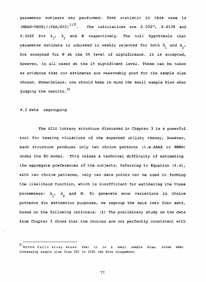
parameter estimate was performed. Test statistic in this case is
1/2 (MEAN-TRUE) / (VAR/6OO) . The calculations are 2.0327, 2.6138 and
0.3466 for hl, h2 and 8 respectively. The null hypothesis that
parameter estimate is unbiased is weakly rejected for both h and h2, 1
but accepted for 9 at the 5% level of significance. It is accepted,
however, in all cases at the 1% significant level. These can be taken
as evidence that our estimates are reasonably good for the sample size
chosen. Nonetheless, one should keep in mind the small sample bias when
2 1 judging the results.
4.3 Data regrouping
The HILO lottery structure discussed in Chapter 3 is a powerful
tool for testing violations of the expected utility theory, however,
each structure produces only two choice patterns (i.e.A?AA or BBBB)
under the EU model. This raises a technical difficulty of estimating
the aggregate preferences of the subjects. Referring to Equation (4.4),
with two choice patterns, only two data points can be used in forming
the likelihood function, which is insufficient for estimating the three
parameters: Al, h2 and 8. To generate more variations in choice
patterns for estimation purposes, we regroup the data into four sets,
based on the following rationale: (1) The preliminary study on the data
from Chapter 3 shows that the choices are not perfectly consistent with
2 1 M o n t e C a r l o s t u d y s h o w s that .it is a small sample bias, since when
increasing sample size from 250 to 2000 the bias disappears.

any theory. Furthermore, choice patterns seem to be sensitive to
lotteries generated from different parts of the Marschak-Machina
triangle. Hence it would be interesting to use data from one portion
to calibrate the model in other portions of the triangle; (2) More than
one data set was needed for testing.
The four data sets summarized in Table 4.1 are also graphically
shown in Figure 4.4. They are labelled I, 11, I11 and IV. For example,
data set I, consisting of pairs 1, 5, 9, is presented by the circle in
the middle of the triangle.
Figure 4.4 also reveals our experimental design, which defines
the precise hypotheses to be tested. The purpose now is to develop a
new approach to test whether a particular theory of choice works
uniformly on the Marschak-Machina triangle, or whether individuals make
consistent choices from one part of the triangle to another under a
particular theory.
4.4 TESTING THE EU MODEL
Our Monte Carlo study shows that the maximum likelihood
technique produces reliable estimates for "artificial consumers1' who
follow the expected utility theory. The question arises: Do real
consumers make decisions under uncertainty in accordance with the
expected utility theory? More generally, how would we know that a
particular model is adequate in explaining the experimental data? To

T a b l e 4 . 1 : T h e D a t a S e t s used for Preference R e c o v e r y
No. of data set Lottery Pairs Involved
Fig.4.4: T h e D a t a S e t s for Preference R e c o v e r y

be able to answer these questions, we construct a test to determine if
subjects consistently follow the expected utility theory. More
specifically, we use each data set to estimate the preferences
density function and the mistake parameter. Since all data sets were
generated from the same population, if the underlying theory is true,
the parameters associated with the preferences function (i.e., Aland
A2) estimated from one set of data should not be significantly
different from another assuming that the subjects were consistent in
making these choices (the rationality assumption). Based on this
argument, a likelihood ratio (LR) test is constructed to test the
hypothesis that these parameters are statistically the same. Should the
null hypothesis not be rejected, we would conclude that the choices
generated under the expected utility theory were from the same
preferences density function. This may indicate the validity of the
theory. Conversely, should the null hypothesis be rejected, the
adequacy of the theory in explaining these choices is questionable.
The LR test statistic is defined as LR=-21117, where z=RL/UL, RL
represents the constrained maximum likelihood value and UL stands for
the unconstrained maximum likelihood value. Given the two parameters
to be tested, there are two restrictions to be imposed for a test
2 between any two data sets. Thus, the LR test statistic follows a X
2 distribution with 2 degrees of freedom. The critical value of X (2) at
the 5% significance level is 5.99. Notice that we do not have a
standard regression equation in which restrictions can be explicitly
imposed in our model. Consequently, calculations of UL and RL are
somewhat different from the conventional method. In particular, lnUL is

the sum of the two maximum log-likelihood values from estimating two
sets of parameters using two data sets; the RL is obtained by pooling
the two sets of data through restricting h 1'
h2, that is, to assume the
2 2 parameters h and h are the same in two data sets.
1 2
Notice that our central hypothesis is that the v values of the
same population in two different experiments are the same. However, if
the hypothesis that the two sets v values are drawn from the same
density function is rejected, then this central hypothesis will also be
rejected. This indicates that individuals under the expected utility
model make inconsistent choices. Therefore the validity of the
underlying theory is questionable. Given this discussion, we conclude
that though the constructed test statistic is biased in testing our
central hypothesis, it is biased in the correct direction if the null
is rejected. However, if the null hypothesis is accepted, it is not
clear that we should immediately accept the theory. In this sense, the
proposed LR test can be considered a test of "false" models not the
"true" model.
Table 4.2 presents the parameter estimates using all data sets.
The test results are reported in Table 4.3. Table 4.2 shows that the
estimates are very different from one set of data to another. In all
22A Monte-Carlo s t u d y was c o n d u c t e d t o t e s t t h e v a l i d i t y o f t h i s test .
F o r 2000 s i m u l a t i o n r u n s , t h e n u l l h y p o t h e s i s was r e j e c t e d a t t h e 5% l e v e l o f s i g n i f i c a n c e f o r 117 t i m e s , t h a t is, 5.85% o f t h e t o t a l
number. T h i s i n d i c a t e s t h a t t h e test i s v a l i d . W e a l s o conduc ted a
Monte-Carlo s t u d y on t h e power o f t h e t e s t . The r e s u l t s show t h a t t h e
power i n c r e a s e s a s w e move f u r t h e r away from t h e n u l l .
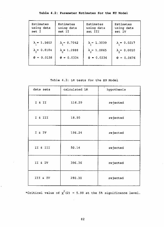
Table 4.2: Parameter Estimates for the EU Model
Estimates Estimates
set I1
Table 4.3: LR tests for the EU Model
data sets I
Estimates using data set 111
*Critical value of
Estimates using data set IV
rejected
calculated LR hypothesis
18.90
rejected
rejected
196.24
50.14
396.36
2 X (2) = 5.99 at the 5% significance level.
rejected
rejected
rejected
cases, as shown in Table 4.3, the null hypothesis that the
parametersare the same is rejected. We suggest three possible
interpretations: First, the beta distribution density function used for
maximum likelihood estimation may be too inflexible (e.g, it is a
unimodal distribution) to approximate the real density function of the
population on the preference parameter v space; second, the expected
utility model is inadequate in explaining individual decisions under
risk.
To focus on the first possibility, we used the experimental
data to generate a histogram or frequency distribution for the subjects
in the v space. We then plotted both the histogram and the estimated
beta distribution on one diagram. In general, the recovered beta
distributions fit the histograms very well. The histograms shows
that all data sets gave rise to unimodal distributions. Figure 4.5
shows examples of the histograms and the recovered beta density
2 3 functions for the subjects. Since we have also shown in the previous
section that the maximum likelihood estimates in the simulation study
are approximately unbiased, we conclude that the assumption of a beta
density function is not responsible for failure of the test.
We therefore conclude that the EU model fails to explain our
data. This is consistent with the results found in all other studies
that people's actual choice behavior is inconsistent with what expected
2 3 T h e s e h i s t o g r a m s a r e c o n s t r u c t e d i n terms of v parameter space only.
Parameter 8 i s b e i n g s e t a t 0.
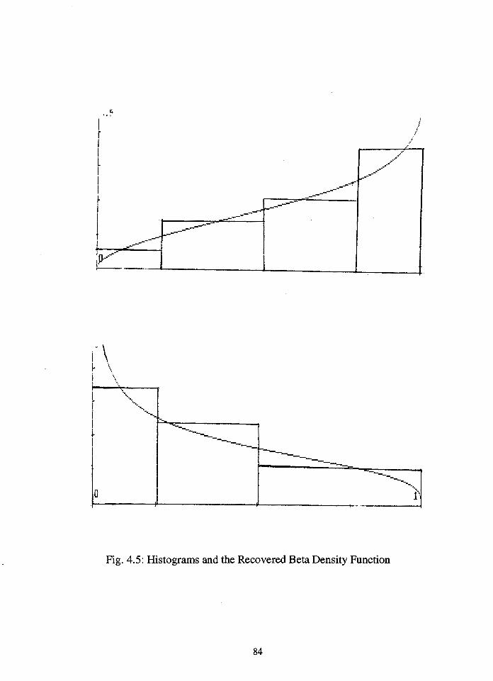
Fig. 4.5: Histograms and the Recovered Beta Density Function

utility theory predicts. The task now is to apply this new testing
technique to alternative models and see if there exists an adequate
theory to explain the experimental data. The next chapter explains
three alternative models and testing results.
4.5 SUMMARY
This chapter presented the preferences recovery techniques for
the EU model. A likelihood ratio test based on recovered preference
density function was provided to test the inadequacy of EU in
explaining the choices people make in laboratory experiments. The
results show that EU fails to predict all our experimental data, even
when we allow for randomness in the model. We then conclude that it is
not an appropriate model for the data.
It should be noted that although the empirical estimation
procedure was presented in terms of a particular example, its
generalization is straightforward. As will be seen in the next chapter,
it can be easily applied to other choice models.

Chapter Five
THE ALTERNATIVE MODELS
As with the other overwhelming evidence from laboratory
experiments reporting that the expected utility model is a poor
descriptor of empirically observed decision making behavior, this study
found further evidence demonstrating the inadequacy of EU in explaining
choices. The question is: Does there exist an alternative theory that
could adequately explain the data? The purpose of this chapter is to
search for such a model. We have seen from the review of literature in
Chapter 2 that, over the past decade, many attempts have been made to
extend the EU model in various ways to improve on the descriptive
ability of the EU model. Roughly speaking, there are two classes of
extensions among the alternative models. One class contains the
subjectively weighted utility (SWU) models where the criterion for
decision making is a weighted sum of the utility index, and the weights
are some transformations of probabilities (Karmarkar, 1978; Quiggin,
1979,). Another class replaces the utility index with some function of
probabilities and final outcomes (Coombs & Huang, 1970; Chew and Dekel,
1979; Machina, 1982). All these models are similar in spirit in that
they are more generalized forms of expected utility and describe
decision behavior in terms of maximization of the criterion. It is not
the purpose of this study to create a new generalized utility theory,
or to justify the existing theories. It is, rather, to search for an
"adequate" theory that explains our experimental data. Two criteria
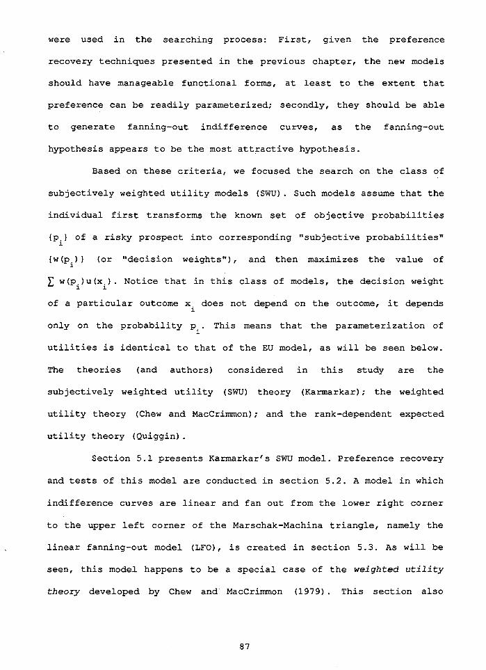
were used in the searching process: First, given the preference
recovery techniques presented in the previous chapter, the new models
should have manageable functional forms, at least to the extent that
preference can be readily parameterized; secondly, they should be able
to generate fanning-out indifference curves, as the fanning-out
hypothesis appears to be the most attractive hypothesis.
Based on these criteria, we focused the search on the class of
subjectively weighted utility models (SWU). Such models assume that the
individual first transforms the known set of objective probabilities
{pi} of a risky prospect into corresponding "subjective probabilities"
{w(pi)} (or "decision weights"), and then maximizes the value of
W (pi) U (xi) . Notice that in this class of models, the decision weight of a particular outcome X does not depend on the outcome, it depends
i
only on the probability p . This means that the parameterization of i
utilities is identical to that of the EU model, as will be seen below.
The theories (and authors) considered in this study are the
subjectively weighted utility (SWU) theory (Karmarkar); the weighted
utility theory (Chew and MacCrimmon); and the rank-dependent expected
utility theory (Quiggin) . Section 5.1 presents Karmarkar's S W model. Preference recovery
and tests of this model are conducted in section 5.2. A model in which
indifference curves are linear and fan out from the lower right corner
to the upper left corner of the Marschak-Machina triangle, namely the
linear fanning-out model (LFO) , is created in section 5.3. As will be
seen, this model happens to be a special case of the weigh ted u t i l i t y
t h e o r y developed by Chew and MacCrimon (1979). This section also

r epor t s t h e test r e s u l t s f o r t h i s model. Section 5.4 in t roduces t h e
rank-dependent u t i l i t y theory proposed by Quiggin (1982 ) . This theory
i s based on a function, f ( P ) , t h a t s a t i s f i e s t h e fol lowing genera l
condi t ions : f (0) =O, f (1/2) =1/2, and f (l) =l. Following t h i s theory, w e
cons t ruct a quadra t ic func t iona l form f o r • ’ (P) i n which t h e above
condi t ions a r e s a t i s f i e d . This model is c a l l e d t h e quadra t ic
rank-dependent (QRD) u t i l i t y model. Test r e s u l t s a r e a l s o provided i n
t h i s s e c t i o n . Sect ion 5.5 p resen t s a t e s t of r e l a t i v e explanatory power
f o r a l l t h e a1ternativ.e models. F inal ly , sec t ion 5.6 makes a concluding
remark.
5.1 KARMARKAR'S SWU MODEL
Karmarkar (1978) proposed a subjec t ive ly weighted u t i l i t y (SW)
model a s a d e s c r i p t i v e extension of t h e EU model. According t o t h i s
model, t h e u t i l i t y f o r a l o t t e r y (p1' P2r P3; XI, X2t X3) i s defined
where
I n t h i s
X -+u
P i - + W
model, p r i z e s a r e mapped i n t o u t i l i t i e s i n t h e usual manner:
( X ) , and p r o b a b i l i t i e s a r e transformed i n t o sub jec t ive weights:
( p . ) a s def ined above. (X i s an addi t ional parameter t h a t may be
regarded a s a measure of p robab i l i ty d i s t o r t i o n . When a=l, t h e SW

model reduces to the EU model. The mapping for various a values is
sketched in Fig. 5.1. For a * 1 the mapping has three fixed points: 0, 1/2, and 1. Thus equiprobability, certainty, and impossibility are not
affected by the mapping. When 0<a<1, W (pi) >pi for p.<1/2, and w(P,) <P,
for p,>1/2. This is known in the literature (e.g., Dale, 1959; Kahneman 1
and Tversky, 1979) as subjects overestimating low probabilities (pi<
1/2) and underestimating high ones. Symmetrically, when 0 1 , w(pi) < p,
for p,< 1/2, and w(pi) > pi for p , > 1/2. This is the case of
overestimating high probabilities and underestimating low ones. Figure
5.2 shows a contour plot of the indifference map of an individual with
v=0.2 and a=0.5.
It is argued by Karmarkar (1979) that this model can be used to
explain the A l l a i s paradox or fanning-out effect. Unfortunately, as
proved by Quiggin (1982), this model violates the stochastic dominance
property of the EU model. When such a property is imposed on
Karmarkar's SWU model, the model reduces to EU. Lottery A is said to
stochastically dominate lottery B if the expected utility from A is
larger than that from B for all monotonically increasing utility index
u(x) . Given the nonlinear probability transformation of the SWU model, Quiggin argued that under certain conditions, a stochastically dominant
24 lottery may generate a lower expected utility. Nonetheless we shall
use our preference recovery techniques and the LR test, to see if this
model could adequately explain our data.
24 For a thorough proof, see Quiggln (1982).
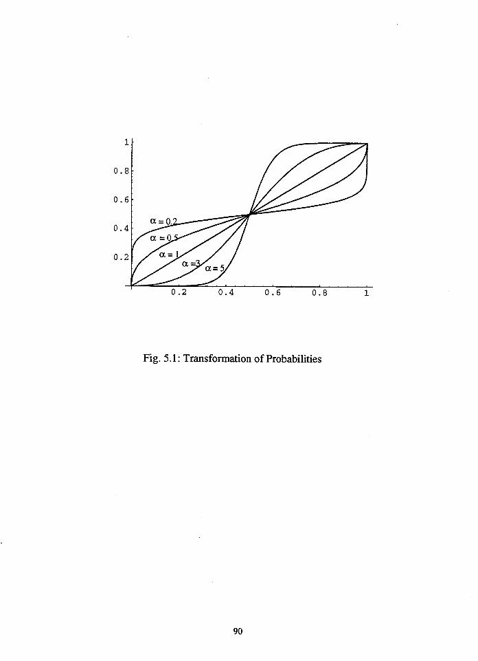
Fig. 5.1 : Transformation of Probabilities

Fig. 5.2: Indifference Curves of the SWU Model

5.2 PREFERENCE RECOVERY AND TEST OF THE MODEL
From equation ( l ) , an individualrs preference over lottery
(plr pZ, p3; X X X ) is completely described by the utility index: 1, 2, 3
u (xl)=l, U (X )=V and U (X )=0 and the additional parameter a. Given the 2 3
value of v derived from a beta distribution and the value of or, the
individualrs subjectively expected utility (SEU) over this lottery can
be calculated by equation (5.1). With two lotteries, he or she picks
the one that gives the higher SEU. As in the EU model, we continue to
assume that there is a probability of 8 that the individual picks the
"wrongtT lottery (i . e. , the one with the lower SEU) . Thus, preference recovery for the alternative model involves estimating four parameters:
the two parameters from beta distribution function h and h2, the 1
mistake parameter 8, and the probability distortion parameter or. For
simplicity, both the mistake parameter and the distortion parameter are
assumed to be the same across individuals. Hence the diversity of
2 5 individual consumers is captured solely by the parameter v.
To estimate the parameters, we construct likelihood functions
of the data sets in exactly the same way as under the EU model, after
transforming the objective probabilities into subjective weights. In
particular, given three pairs of lotteries, a typical set of data
2 5 O n e c o u l d a s s u m e t h a t t h e additional parameter for each alternative
model is different from individual to individual. In this case, the
subjects are considered to be drawn from a joint density function
f (v,z; A), where z represents the additional parameter in each model,
h is a set of unknown parameters to. be estimated.
presented in Chapter 4, and with each lottery represented by (p 1' P2'
P3; X 1' X 2' x i ) , there are eight choice patterns generated from a
sample population. Let Q(j) be the number of subjects choosing choice
pattern j, j=1, ......, 8. Given a beta distribution density function f (V; A A ) and parameters 8 and a, the probability of generating each
1' 2
of the eight choice patterns, Rj(Al,A2.~.a), is calculated. The
likelihood function of generating the data is given by
The estimates are obtained by maximizing L (A ,A ,@,a) . 2 6 1 2
Using all four data sets: I, 11, 111, IV (for convenience, Fig.
4.4 with data sets circled on the Marschak-Machina triangle is shown as
Fig. 5.3 in this chapter), we estimated the preference density
functions and performed the LR test for the SWU model. The test
statistic has 3 degrees of freedom instead of 2 due to the additional
2 parameter a. The critical value of X (3) at the 5% significance level
is 7.81. The test once again, was used to test the hypothesis that the
parameters A A and a estimated using one set of data are the same as 1, 2
those estimated using another data set.
2 6 T h e c o m p u t e r p r o g r a m s f o r these alternative models written in FORTRAN are also available from the author.
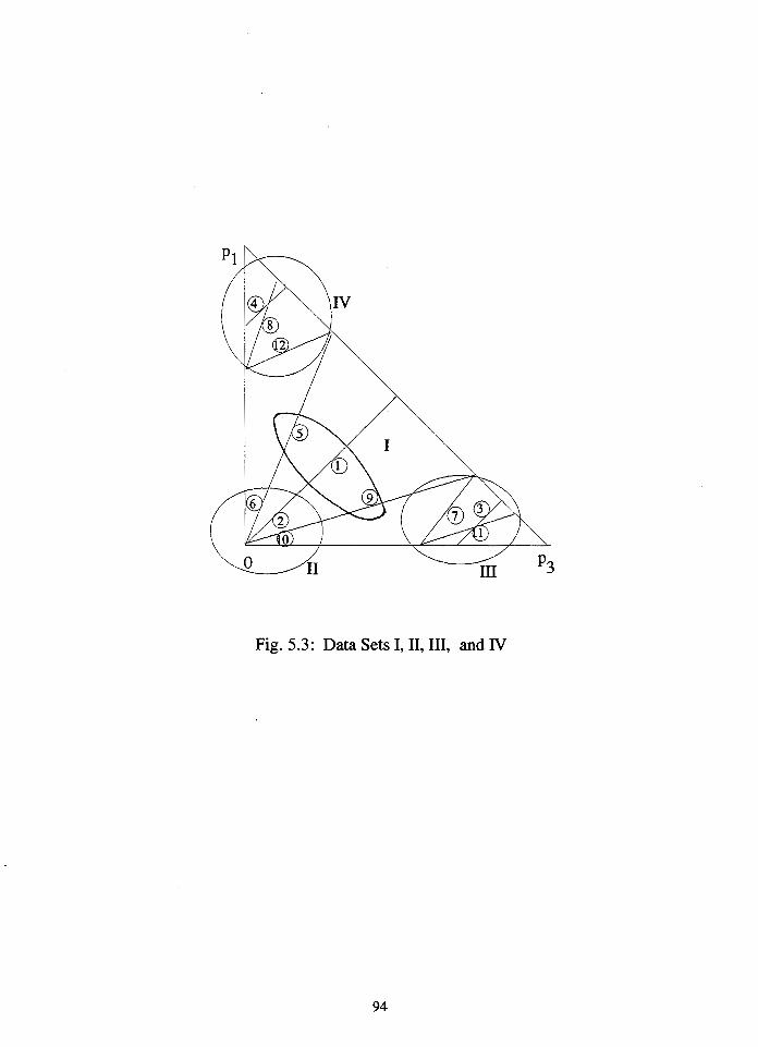
Fig. 5.3: Data Sets I, 11,111, and IV

Parameter estimates are reported in Table 5.1 and test results
are provided in Table 5.2. Table 5.1 shows that the parameter estimates
for AI, A*,
and a vary significantly from one set of data to another.
Estimates for the mistake parameter 8, however, remain small and
relatively stable. It is interesting to note that the estimate of a is
1 in data set IV and nearly 1 in data set 111. This means that the SWU
model does not improve on EU in these regions since the model reduces
to EU when a=l. The estimate from data set I1 (a=0.42) indicates that
on average the subjects overestimate low probabilities and
underestimate high ones in the neighborhood of certainty (the area
around the origin and inside the triangle) - a case commonly reported
in the literature. But the estimate from set I (a=4.37) shows the
opposite. It is not clear what causes these disparate results. Table
5.2 shows that the null hypothesis is rejected in all cases except for
data sets I and 111. In the context of five rejections, the one
acceptance could be interpreted as a type I1 error. This argument is
supported by comparing the estimates from data set I (A = 0.27, - 1 A2-
0.11, 8=0.01, a=4.37) and those from data set I11 (A = 1.30, h = 1.09, 1 2
8=0.02, a=1.01). Since they appear different, the hypothesis that these
parameters are the same should not be accepted even with visual
inspection.

Table 5.1: Parameter Estimates for the S W Model
Estimates using data set 111
Estimates using data set I
~stimates using data set IV
Estimates using data set I1
Table 5.2: LR tests for the S W Model
Data sets
I & I1
I & I11
I & IV
I1 & I11
Calculated LR
117 - 2 0
3.46
I1 & IV
2 Critical value of X (3) = ' 7 . 8 1 at the 5% significance level.
Hypothesis
rejected
accepted
197.08
31.76
I11 & IV
rejected
rejected
398.52 rejected
281.26 rejected
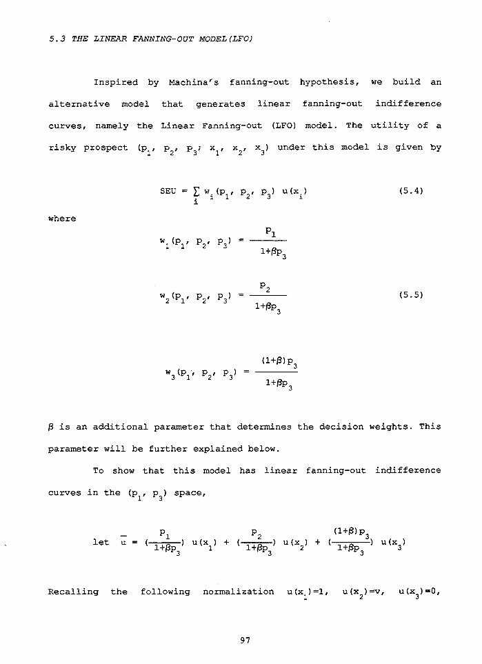
5.3 THE L I N E A R FANNING-OUT MODEL (LFO)
Inspired by Machinars fanning-out hypothesis, we build an
alternative model that generates linear fanning-out indifference
curves, namely the Linear Fanning-out (LFO) model. The utility of a
risky prospect (pl, p2, p,; X X X ) under this model is given by 1, 2, 3
where
W, (P,, P, I P,) = P1
~+BP,
w2(p1r P2r P,) = P 2
~+BP,
6 is an additional parameter that determines the decision weights. This
parameter will be further explained below.
To show that this model has linear fanning-out indifference
curves in the (pl, p,) space,
Recalling the following normalization U (X ) =l, U (X ) =v, U (x3) =O, 1 2
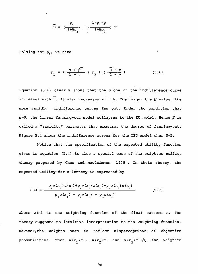
Solving for p we have 1
Equation (5.6) clearly shows that the slope of the indifference curve
- increases with U. It also increases with p. The larger the (3 value, the
more rapidly indifference curves fan out. Under the condition that
6=0, the linear fanning-out model collapses to the EU model. Hence (3 is
called a "rapidity" parameter that measures the degree of fanning-out.
Figure 5.4 shows the indifference curves for the LFO model when 6=5.
Notice that the specification of the expected utility function
given in equation (5.4) is also a special case of the w e i g h t e d u t i l i t y
theory proposed by Chew and MacCrimmon (1979) . In their theory, the expected utility for a lottery is expressed by
p w(x )u(x )+p w(x )u(x2)+p3w(x3)u(x3) 1 1 1 2 2
SEU =
where w(x) is the weighting function of the final outcome X. The
theory suggests no intuitive interpretation to the weighting function.
However,the weights seem to reflect misperceptions of objective
probabilities. When W (xl) =l, . W (X ) =l and W (X ) =1+/3, the weighted 2 3

Fig. 5.4: Indifference Curves of the LFO Model

utility model becomes the LFO. ~otice that from equation (5.7), these
decision weights depend upon both the probabilities and outcomes that
determine the utilities, while in the class of the subjectively
weighted utility models decision weights (i.e., w(p)) depend on only
probabilities, p.
Preference recovery for the LFO model involves estimating h 1,
h*, 8, and p. Using the same method and procedure described for the SWU
model, we estimate these parameters and test the adequacy of the LFO
model in explaining our data. The results are shown in Tables 5.3 and
5.4. Table 5.3 shows that the estimated hl and hp for the LFO model
vary significantly from one data set to another, and that both the
mistake parameter and the additional parameter 6 are estimated to be
very small. A small indicates a small degree of fanning-out
indifference curves. As presented in Table 5.4, the null hypothesis is
rejected for all data sets for the LFO model. The LR values are almost
the same as those calculated for the EU model for data sets I & I1 and
I and 111. But The LR values for the other four data sets are much
smaller than those calculated for the EU model, indicating some
improvements. However, they are not small enough to accept the null
hypothesis. Therefore the LFO model is also not an appropriate model
for explaining the data.
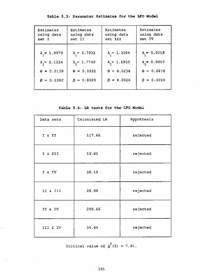
Table 5 . 3 : Parameter Estimates for the LFO Model
Estimates using data set I
Estimates using data set I1
Estimates using data set I11
Estimates using data set IV
Table 5 . 4 : LR tests for the LFO Model
Data sets I rejected
Calculated LR
rejected
Hypothesis
rejected
rejected
Critical value of XL ( 3 ) = 7.81.
250.66
54.84
rejected
rejected
5.4 THE QUADRATIC RANK-DEPENDENT U T I L I T Y MODEL ( Q m )
I n most of t h e s u b j e c t i v e l y weighted u t i l i t y models such a s t h e
one c r e a t e d by Karmarkar i n s e c t i o n 5.1, t h e d e c i s i o n weight w(p . ) of 1
outcome X depends on only t h e p r o b a b i l i t y p . Thi s means t h a t outcomes i i
wi th t h e same p r o b a b i l i t y must have t h e same d e c i s i o n weight. Quiggin
(1992) proposed a rank-dependent u t i l i t y theory ( i n i t i a l l y c a l l e d t h e
a n t i c i p a t e d u t i l i t y t heo ry ) i n which t h e p r o b a b i l i t y t r ans fo rma t ion of
pi n o t on ly depends on p . bu t a l s o depends on p r o b a b i l i t i e s of o t h e r l.
outcomes. I n p a r t i c u l a r , t h e t ransformat ion func t ion W , (p ) depends on 1
a l l p f o r j s i . According t o t h i s theory, t h e expected u t i l i t y of a j
where,
• ’ (p ) i s a t ransformat ion func t ion of l o t t e r i e s wi th only two outcomes.
It i s used he re t o form t h e weights w . (p ) f o r l o t t e r i e s i nvo lv ing t h r e e 1
outcomes. Quiggin d i d not suggest a s p e c i f i c form f o r f (p) i n h i s
paper, bu t he d i d d i s c u s s t h e genera l p r o p e r t i e s of t h i s func t ion . I n
p a r t i c u l a r , f (p) determines t h e p a t t e r n of p r o b a b i l i t y d i s t o r t i o n .

f (p )>p f o r p<1/2 and f ( p ) < p f o r p>1/2 imply t h a t s u b j e c t s overes t imate
smal l p r o b a b i l i t i e s and underest imate h igh ones. More s t r i c t l y , t h i s
c a s e r e q u i r e s t h a t f (p) i s concave on [O, 1/21 and convex on [1/2, l ] ,
and t h a t f (O)=O, f (1/2)=1/2, f (1)=1. This echoes t o Karmarkar's
d e c i s i o n weights f u n c t i o n with 0<a<1.
According t o t h i s genera l d e s c r i p t i o n of f ( p ) , we c r e a t e a
27 q u a d r a t i c func t ion a s fo l lows
f o r 0 < p 5 112
f ( p ) =
(7-1) + (4-3%) p+2 (T-1) P f o r 1 / 2 s p s l
and s a t i s f y i n g t h e r e s t r i c t i o n s ,
The parameter a' measures t h e d i s t o r t i o n of o b j e c t i v e p r o b a b i l i t i e s .
When y > l r f ( p ) i s concave on [ O , 1/21 and convex on [1/2, l], When
O<;r<l, f (p) i s convex on [ O , 1/21 and concave on [1/2, l ] . When ;r-l,
t h e r e i s no d i s t o r t i o n .
P u t t i n g f (p) i n t o equat ion (5.9), w e o b t a i n a ve r s ion of t h e
rank-dependent u t i l i t y model, namely t h e q u a d r a t i c u t i l i t y func t ion
(QRD) . Given t h e d e f i n i t i o n of f (p) , EU i s a s p e c i a l ca se of QRD when
27 L a t e r on, w e f o u n d f r o m a recent book (1992) Quiggin wrote that
Camerer and H0 ( 1 9 9 1 ) employed and estimated the following functional
7 a' 1 / 2 form: f ( p ) = p (p + ( l - p ) ) .

y=1. As illustrated in Figure 5.5, the indifference curves of the QRD
model for 7=1.5 are nonlinear and fan out from the lower right corner
to the upper left corner of the triangle.
Table 5.5 shows the estimates for all four data sets. Once
again, the estimates for A and A differ significantly from one set of 1 2
data to another. The mistake parameter remains the same as in all
other models. The estimated y, however, shows that on average subjects
underestimate small probabilities (or overestimate high ones) in region
I (y=0.2 ) and region IV (y=0.41) , and overestimate small probabilities
(or underestimate high ones) in region I1 (~=3.01) and region I11
(7~1.12). The non-linear fanning-out is thus observed in regions I1 and
111.
Table 5.6 reports the test results of this model. Once again,
we see rejections of the hypothesis for all data sets. The difference
between this set of results and those found for the EU model is the
case for data sets I & 111, and I1 and 111. The LR values for the QRD
model are smaller than those for the EU model. One final interesting
observation from Tables 5.1, 5.3, 5.5 and 4.1, is that the estimated 8
is approximately the same across all models using the same data set.
Since 8 measures the probability of choosing the less-preferred lottery
under each model, the result indicates that the probability of an
individual making a mistake is quite consistent across all theories.
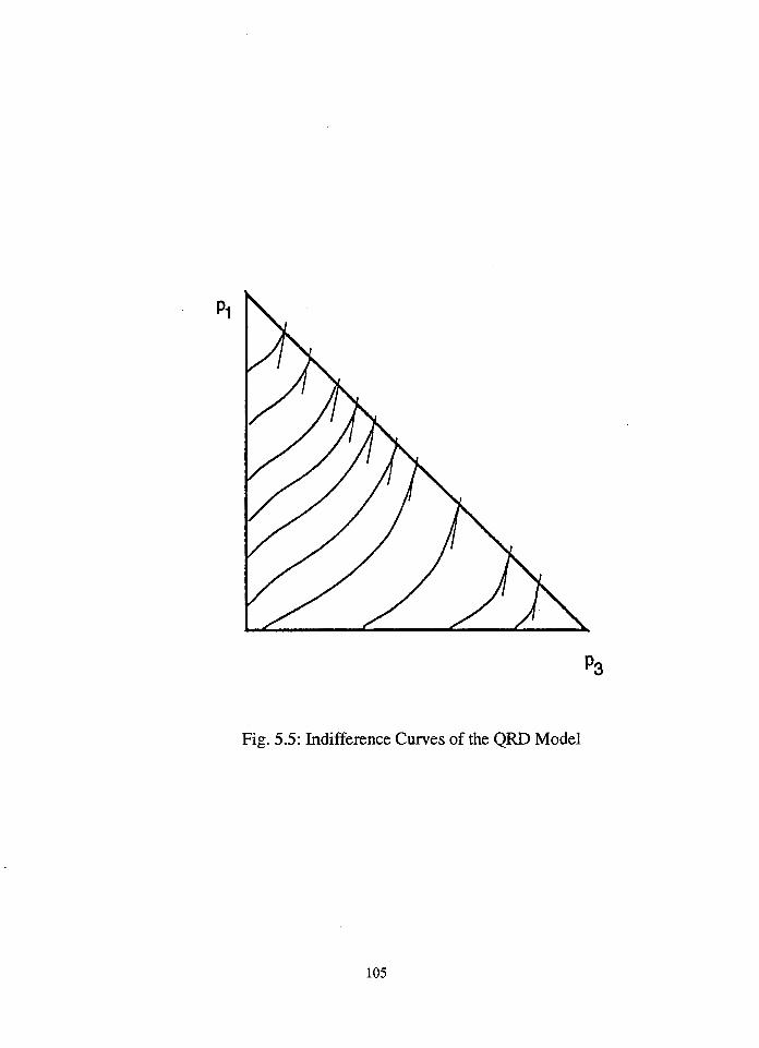
p3
Fig. 5.5: Indifference Curves of the QRD Model

Table 5.5: Parameter Estimates for the QRD Model
Estimates using data set I
Estimates Estimates Estimates using data using data using data set I1 set 111 set IV
Table 5.6: LR tests for the QRD Model
Data sets
I & I1
I & I11
I & IV
I1 & I11
I1 & IV
I11 & IV
2 Critical value of X (3) = 7.81.
Calculated LR
115.56
11.82
185.84
30.08
356.12
125.26
Hypothesis
rejected
rejected
rejected
rejected
rejected
rejected

5.5 A TEST OF MODEL PERFORMANCE
As discussed in the previous sections, all the alternative
models include EU as a special case. In particular, when a=l, SWU
becomes EU; when p=0, LFO converts into EU; and when ~ = 1 , the QRD
models collapses to the EU model. To test if these alternative models
are improvements on EU, one can perform a LR test of these
restrictions. For example, the LR test of hypothesis, Ho:a=l, for the
SWU model is LR=-2 (1nRL-lnUL) , which asymptotically has a I C ~ (1)
distribution. lnRL is the maximum log-likelihood value under the null
hypothesis, lnUL is the maximum log-likelihood value under the
alternative model. Acceptance of this hypothesis would, of course,
imply that the alternative model does not add more explanatory power to
the EU model, empirically.
Table 5.7 presents the LR tests of relative explanatory power
of the alternative models for all data sets. The numbers in parentheses
2 are the calculated LR values. The critical value of K (1) at the 5%
significance level is 3.84. The results show that the null hypothesis
under each model is accepted for all data sets. Therefore, these
alternative models are not improvements on EU for our data.
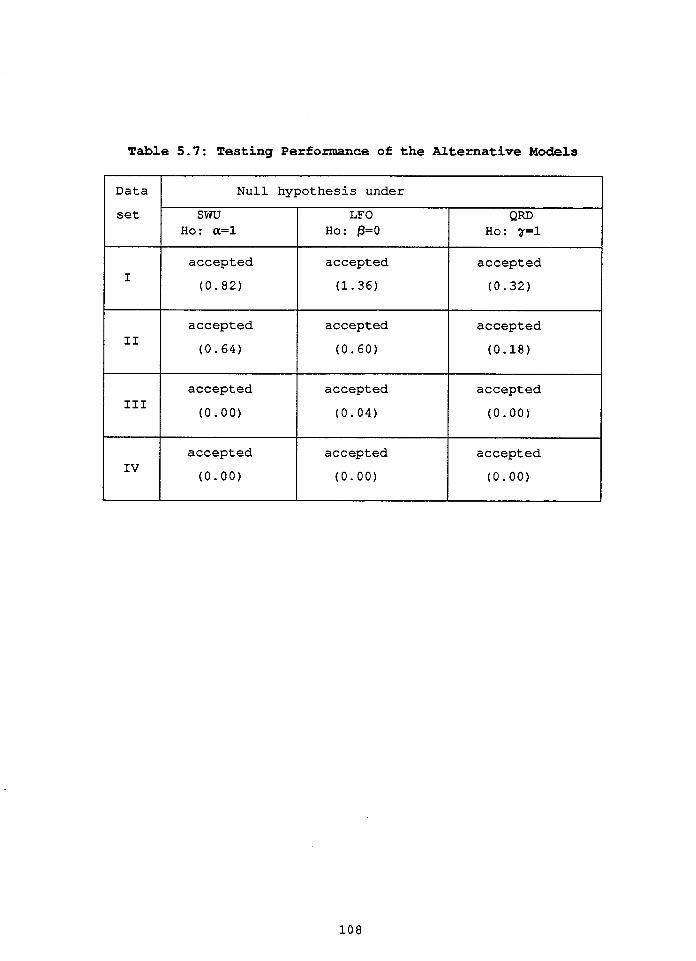
Table 5.7: Testing Performance of the Alternative Models
Data.
set
I
accepted
Null hypothesis under
I I I
SWU Ho: a=l
accepted
(0.82)
accepted
accepted
I I l
accepted
accepted
LFO Ho: p=0
accepted
(1.36)
accepted
QRD Ho: 7=1
accepted
(0. 32)
accepted
accepted accepted
5.6 CONCLUDING REMARKS
This chapter has presented t h r e e a l t e r n a t i v e func t iona l forms:
one from e x i s t i n g l i t e r a t u r e and t h e o ther two c r e a t e d by t h e author.
inadequacy tests w e r e performed on t h e a l t e r n a t i v e models using t h e
same data sets. The r e s u l t s show t h a t no theory can exp la in a l l t he
d a t a sets. Furthermore, a test of r e l a t i v e performance of these
a l t e r n a t i v e models a s compared t o t h e EU model shows t h e a l t e r n a t i v e
models a r e not s i g n i f i c a n t improvements on t h e EU model. Therefore we
conclude t h a t t h e t h r e e a l t e r n a t i v e models, each with an add i t iona l
parameter, do not add much explanatory power, and t h a t u n t i l w e f i n d a
model t h a t passes a l l adequacy tests, t h e expected u t i l i t y theory,
charac ter ized by i t s s impl ic i ty and normative appeal of i t s axioms,
r e t a i n s i t s leading r o l e i n t h e o r i e s of choice under uncer ta in ty .
Chapter Six
ANOTHER ILLUSTRATION
The previous chapters presented a new approach t o t e s t i n g
t h e o r i e s of choice under uncer ta in ty . In t h e approach it i s assumed
t h a t ind iv idua l s under a p a r t i c u l a r theory of choice have d ive r se
preferences described by po in t s i n a parameter v-space, v E [0,11.
Aggregate preferences of a sample population a r e represented by a
p r o b a b i l i t y d i s t r i b u t i o n funct ion of v . To study t h e aggregate choices
people make over a set of d i f f e r e n t i a t e d products (e .g. , l o t t e r i e s ) ,
one needs t o es t imate such a p robab i l i ty dens i ty funct ion . This way of
desc r ib ing t h e heterogeneous preferences across ind iv idua l s i s the
s p i r i t of a l l address models of product d i f f e r e n t i a t i o n .
To extend t h e ana lys i s , we demonstrate, i n t h i s chapter , t h e
preference recovery techniques i n a simple but s tandard address model
of product d i f f e r e n t i a t i o n . W e a l s o apply the techniques t o a r e a l case
of product d i f f e r e n t i a t i o n . Section 6 . 1 introduces t h e address model
i n which t h e consumer's preference t akes a known parametric form. It
a l s o o u t l i n e s a genera l procedure f o r es t imat ing t h e aggregate
preference dens i ty funct ion . Section 6 .2 i l l u s t r a t e s an app l i ca t ion t o
a r e a l case of product d i f f e r e n t i a t i o n i n t h e context of BC f e r r y
s e r v i c e s . Sect ion 6 . 3 r epor t s the es t imat ion and out-of-sample t e s t i n g
r e s u l t s . The l a s t s e c t i o n d iscusses t h e p o t e n t i a l l i m i t a t i o n s of t h e
model and provides d i r e c t i o n s f o r f u r t h e r research.

6.1 THE MODEL
Consider a market f o r M d i f f e r e n t i a t e d p roduc t s which a r e
completely desc r ibed by t h e q u a n t i t i e s of K c h a r a c t e r i s t i c s o r
a t t r i b u t e s embodied i n them. L e t t h e M v a r i a n t s be W W 2 r W),,
where W . = ( w W ..., W , = , , M The c h a r a c t e r i s t i c s space i s 3 j l r j2 ' j K
denoted $, t hen W . E l#. Product j i s o f f e r e d f o r s a l e a t p r i c e p 20. 3 j
Suppose t h e r e i s a f i n i t e number of consumers, N, each of whom
i s a p o t e n t i a l customer i n t h e market under d i s c u s s i o n . It i s assumed
t h a t each consumer buys a t most one u n i t of one v a r i a n t of t h e M
p roducts . The p re fe rence f o r v a r i a n t j by an i n d i v i d u a l i i s given by 2 8
W = amount of a t t r i b u t e k (k=l, . . . , K ) pos se s sed by v a r i a n t j j k
( j = l , . . . , M ) .
U = consumer i r s most p r e f e r r e d a t t r i b u t e k r ega rd ing t o h i s i k
o r h e r i d e a l brand s i n c e , when a l l p r i c e s a r e equa l
W.= U maximizes n e t u t i l i t y g iven i n Equat ion 6.1. 3 i
c = a p o s i t i v e cons t an t , measuring t h e marg ina l d i s u t i l i t y k
from no t buying t h e i d e a l brand w i t h r e s p e c t t o
a t t r i b u t e k ( I n t h e geographica l con tex t , t h i s d i s u t i l i t y
28 T h i s p a r t i c u l a r s p e c i f i c a t i o n o f t h e u t i l i t y f u n c t i o n h a s been u s e d i n
s e v e r a l models o f p r o d u c t d i f f e r e n t i a t i o n (see, e .g . , Ea ton a n d
Wooders, 1985.) .
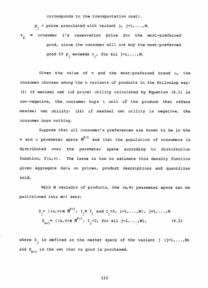
corresponds t o t h e t r a n s p o r t a t i o n c o s t ) .
P j = p r i c e a s s o c i a t e d wi th v a r i a n t j , j=1,. . . , M .
v = consumer i t s r e s e r v a t i o n p r i c e f o r t h e most-preferred i
good, s i n c e t h e consumer w i l l no t buy t h e mos t -prefer red
good if p . exceeds v f o r a l l j= l , . . . , M. 3 i r
Given t h e va lue of v and t h e most-preferred brand U, t h e
consumer chooses among t h e n v a r i a n t s of p roducts i n t h e fo l lowing way:
(i) i f maximal n e t (of p r i c e ) u t i l i t y c a l c u l a t e d by Equat ion (6.1) i s
non-negative, t h e consumer buys 1 u n i t of t h e product t h a t o f f e r s
maximal n e t u t i l i t y ; (ii) i f maximal n e t u t i l i t y i s nega t ive , t h e
consumer buys no th ing .
Suppose t h a t a l l consumer's p re fe rences a r e known t o be i n t h e
v and u parameter space and t h a t t h e popula t ion of consumers i s
d i s t r i b u t e d ove r t h e parameter space accord ing t o d i s t r i b u t i o n
func t ion , f (u ,v) . The i s s u e is how t o e s t i m a t e t h i s d e n s i t y func t ion
g iven aggrega te d a t a on p r i c e s , product d e s c r i p t i o n s and q u a n t i t i e s
s o l d .
With M v a r i a n t s of p roducts , t h e (u,v) parameter space can be
p a r t i t i o n e d i n t o m+1 sets:
S .= { (U, V ) E cl; I,? I and I , > O , i = l , . . . , M ) , j = l , . . . , M 3 3 i 3
S = { ( u , v ) E c'; I . < O I f o r a l l j=1, ..., M } , m+l 3
(6.2)
where S i s d e f i n e d a s t h e market space of t h e v a r i a n t j ( j= l , . . . ,M) j
and SM+l i s t h e set t h a t no good i s purchased.

These sets are illustrated in Figure 6.1 for some arbitrary
prices and product descriptions in the M=3 and K=l case. Given the
number of consumers who have purchased one unit of variant j, the data
provides what amounts to a histogram associated with the unknown
distribution function. The statistical problem is then to recover such
a distribution function from the histogram. Following the previous
chapters, we adopt the maximum likelihood approach to estimate f(u,v).
In order to apply the maximum likelihood estimation technique,
we need to specify a functional form for f (u,v;A), where h is a set of
unknown parameters to be estimated associated with the distribution
function. For instance, if (u,v) is multi-variant normally and
independently distributed in p1 with f (U, v) =MVN (P, Q ) , the unknown - -
parameters to be estimated are the mean vector P=(; 1' "
U V) and the K
variance matrix Q defined as
- - - Thus, A = (ul, .. .,uK, V, cl, . . . , 0. CV)-
NOW, let Q( j) be .the number of units of the jth product
purchased by a sample population. The likelihood function for such a
sample population is expressed by

S1= { ( u , v ) , ue (0, A l ) . end v-c (U-W ) 22pl ) 1
2 S = I ( u , v ) , u E ( A 1 . A 2 ) , and v - c ( u - W ) Z p l
2 2 2
2 S3= { ( u , v ) , u e ( A 2 , A ) , and v - c ( u - W ) rp 1
3 3 - 2
S = { ( U , V ) , UE (0. U) , and v-c (U-W. ) <p i=l , . . . ,4 1 4 1 i
Fig.6.1: The Market Space of Each Product

where R.(A) represents the probability that good j is purchased for 3
j=l,. . .,M, and RM+l (h) is the probability of not buying any product.
Thus,
2 9 s is the market space of product j given in (6.2). j
The maximum likelihood estimates of h is obtained by maximizing
L (h) . Therefore f (U, v) is recovered.
6.2 An Application to BC Ferries
For many years, local residents have petitioned the Government
for improved service. In an effort to meet the needs of the Powell
River community, the Government agreed to expand the sailing schedule
on a trial basis during the 1992 summer period (June 26th to September
8th). Prior to the implementation of the new schedule, there were four
trips per day from Powell River on the Sunshine coast of British
Columbia to Comox on Vancouver Island. The expanded summer schedule
added one additional trip for a total of five sailings per day.
In this particular application, we focus our analysis on this
particular route because it allows us to conduct out-of-sample testing
of the model. Specifically, we will use 1991 data to estimate the
*'Note t h a t i n most p o t e n t i a l applications, U and v are bounded. Thus
f (u,v) is a truncated distribution.
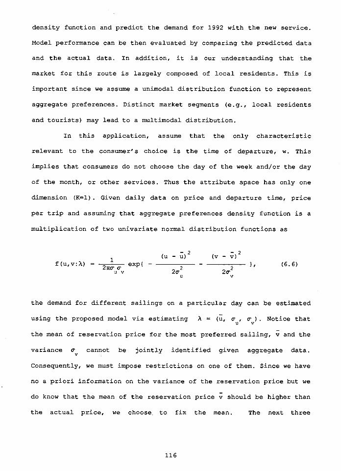
density function and predict the demand for 1992 with the new service.
Model performance can be then evaluated by comparing the predicted data
and the actual data. In addition, it is our understanding that the
market for this route is largely composed of local residents. This is
important since we assume a unimodal distribution function to represent
aggregate preferences. Distinct market segments (e.g., local residents
and tourists) may lead to a multimodal distribution.
In this application, assume that the only characteristic
relevant to the consumer's choice is the time of departure, W. This
implies that consumers do not choose the day of the week and/or the day
of the month, or other services. Thus the attribute space has only one
dimension (K=l). Given daily data on price and departure time, price
per trip and assuming that aggregate preferences density function is a
multiplication of two univariate normal distribution functions as
the demand for different sailings on a particular day can be estimated
- using the proposed model via estimating h = (U, cur 5) . Notice that
the mean of reservation price for the most preferred sailing, and the
variance cannot be jointly identified given aggregate data. v
Consequently, we must impose restrictions on one of them. Since we have
no a priori information on the variance of the reservation price but we
do know that the mean of the reservation price v should be higher than the actual price, we choose to fix the mean. The next three

sub-sections r epor t data, es t imat ion and out-of-sample t e s t i n g r e s u l t s .
6.2.1 Data
The da ta obtained from B.C. Ferry Corporation c o n s i s t s of d a i l y
veh ic le volumes depar t ing from Powell River t o Comox f o r each depar ture
time and each day of the month i n August 1991 and 1992. Since t h e d a i l y
average s i z e i s r a t h e r small and s ince we a r e i n t e r e s t e d i n
out-of-sample p red ic t ions with respect t o some represen ta t ive per iod of
time not s o much with respect t o a p a r t i c u l a r day of t h e month, we have
increased the sample s i z e by aggregating t h e da ta i n such a way t h a t
veh ic le volumes of each s a i l i n g f o r a l l Mondays, Tuesdays e t c . of
August 1991 were summed up (see Table 6 .1 ) . The same aggregation method
has been adopted f o r August 1992. Thus t h e empirical es t imat ion uses
t h e aggregate d a t a f o r August 1991 a s repor ted i n Table 6.1 but not t h e
30 d a i l y da ta . F ina l ly , t h e p r i c e pe r s a i l i n g i s f l a t a t a r a t e of $20
p e r veh ic le .
6.2.2 Monte-Carlo Study
Given t h a t t h e only c h a r a c t e r i s t i c i s t i m e of depar ture ( W ) ,
and t h e p r i c e i s f ixed a t $20, t h e preference dens i ty funct ion given i n
(6.6) can be est imated using the aggregate da ta from Mondays t o Sundays
30 T h i s a g g r e g a t i o n i s c o n s i s t e n t w i t h our assumption t h a t consumers
choose t h e t i m e o f d e p a r t u r e only. Holiday i s excluded i n t h e
aggrega t ion .
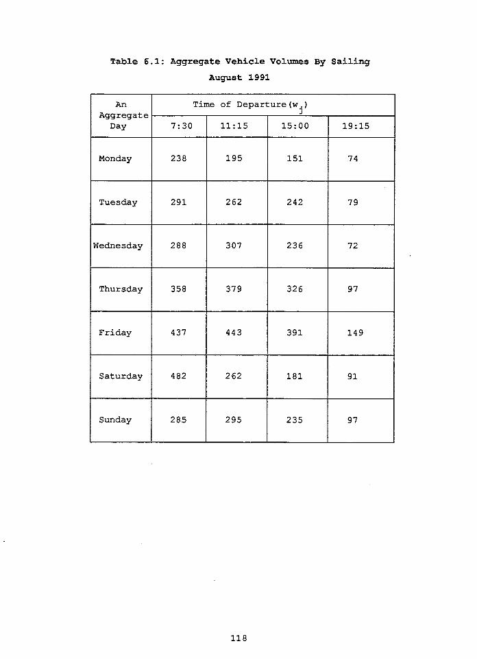
Table 6.1: Aggregate Vehicle Volumes By Sailing
August 1991
An Aggregate Day
Time of Departure (W+
Monday
Tuesday
Wednesday
Thursday
Friday
Saturday
Sunday

- of August 1991. To do so, we need to choose a value for v, the mean
reservation price. Given the actual price at $20 per trip, We fixed
arbitrarily at $25. The parameter c is also fixed at 1 for simplicity.
We also need the potential population for this service since our model
includes a no-set, that is, the number of people who were active in the
market but did not take any sailing. Based on the data summarized in
3 1 Table 6.1, we fixed the population at 1500 vehicles per aggregate day.
The maximum likelihood estimates of A are obtained using an
algorithm that contains a well-known and widely available (IMSL
routines) Quasi-Newton nonlinear optimization routine. Monte-Carlo
studies were conducted to examine the quality of the estimates. In
- - particular, we chose a set of parameters (e.g., U = 10.0, v = 25.0, c =
U
5.0, cr =10.0) as "true" parameters in f (u,v). We then used a random v
3 2 number generator to draw 1500 pairs of (u.v) from this distribution.
Putting each pair of (u.v) into (6.1) and using 1991 prices as well as
departure times, we generate 1500 utility-maximizing choices, which are
aggregated to obtain the simulated vehicle volumes per sailing. Using
this data and our estimation program, we obtain one set of parameter
estimates. By repeating the process for 100 times, we generated 100
sets of parameter estimates. Table 6.2 reports the sampling mean and
3 1 N o t e t h a t t h e a s s u m p t i o n s about the mean of reservation price, the
marginal utility parameter c and the potential population do affect
the distribution of v but not U. Monte-Carlo studies show that these
numbers are within the range that the probability predictions of each
sailing are insensitive to choices of these values.
32 This number is chosen so as t o correspond to the potential population
for each aggregate day.
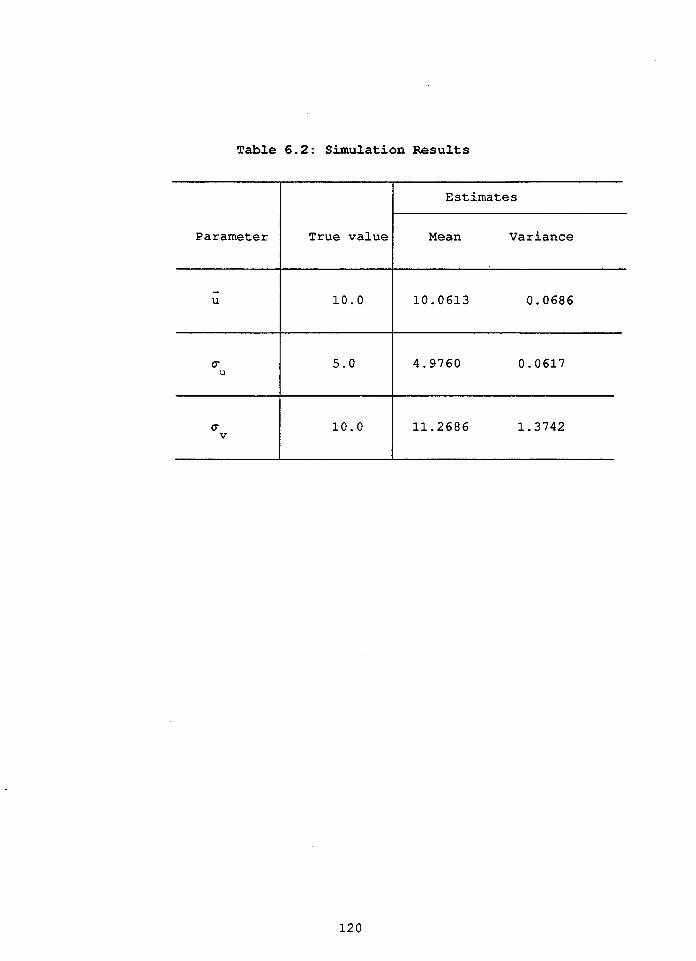
Table 6.2: Simulation Results
Parameter
Estimates
True value Mean Variance

var iance of these es t imates . The hypothesis of e q u a l i t y between t h e
mean and t h e " t rue" values was t e s t e d using a s tandard normal test. The
r e s u l t s show t h a t t h e n u l l hypothesis i s accepted f o r parameter c , but U
weakly r e j e c t e d f o r and 5 a t t h e 5% s ign i f i cance l e v e l . Given t h e
sample s i z e , w e consider t h e es t imates a s being acceptable.
The aggregate preferences dens i ty function i s es t imated using
1991 d a t a given i n Table 6.1. Table 6 . 3 p resen t s t h e es t imat ion
r e s u l t s . I t suggests t h e following: Mondays and Saturdays a r e obviously
d i f f e r e n t from t h e o the r aggregate days of t h e week. I n p a r t i c u l a r ,
they both have a much f l a t t e r d i s t r i b u t i o n of U than t h e o the r days. I n
comparison, Tuesdays, wednesdays, Thursdays and Sundays look very
s i m i l a r with a mean of t h e most p re fe r red depar ture t i m e ( 1 around
mid-day and a r e l a t i v e l y small variances.
6.2.3 Out-Of-Sample Testing
Now we have t h e underlying aggregate preferences f o r each
aggregate day of t h e week , w e can then use t h i s t o p r o j e c t t h e
corresponding veh ic le volumes f o r 1992. I n doing s o w e assume of course
t h a t consumer's preferences a r e s t a b l e over t i m e . Table 6.4 r epor t s t h e
p red ic ted and a c t u a l veh ic le volumes f o r each aggregate day of t h e week
33 i n August 1992.
The p r e d i c t i v e a b i l i t y of t h e proposed model i s examined by
3 3 T h e p o t e n t i a l p o p u l a t i o n of each aggregate day for 1992 is also set
at 1500.

Table 6.3: Parameter Estimates Using 1991 Data
Days
Mondays 7.17 9.52 8.09
Tuesdays 12.82 4.90 11.85
Wednesdays 12.91 4.44 10.74
Thursdays 12.87 4.65 3.29
Fridays 13.46 4.64 12.29
Saturdays 5.57 9.03 2.25
Sundays 12.95 4.98 8.56
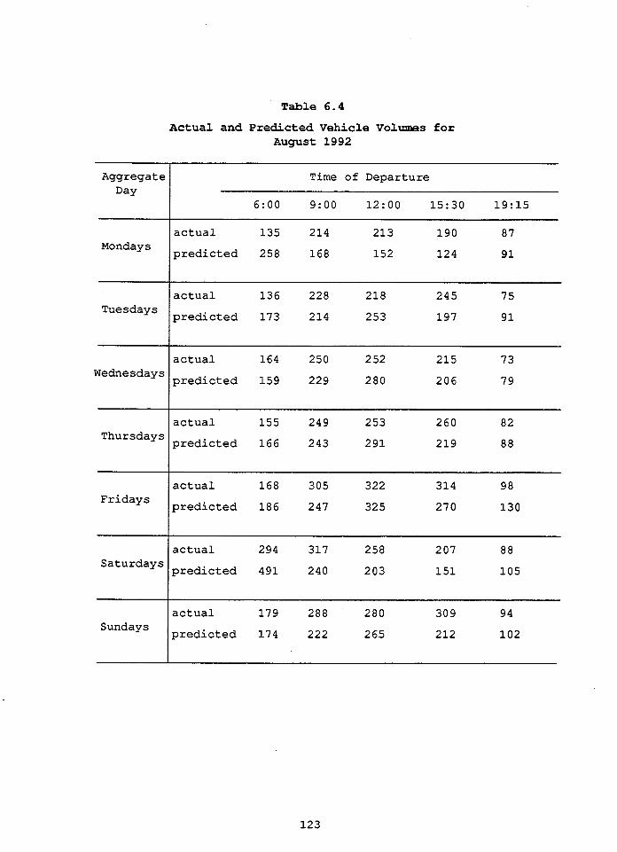
Aggregate Day
Monday S
Tuesdays
Wednesdays
Thursday S
F r idays
Sa turdays
Sundays
T a b l e 6 . 4
A c t u a l and P r e d i c t e d V e h i c l e Volumes for A u g u s t 1992
T i m e of Departure
6:OO 9:OO 12 : 00 15:30 19:15
a c t u a l 135 2 14 213 190 8 7
p r e d i c t e d 258 168 152 124 91
a c t u a l 136 228 218 245 7 5
p r e d i c t e d 173 214 253 197 91
a c t u a l 164 250 252 215 7 3
p r e d i c t e d 159 229 280 206 7 9
a c t u a l 155 249 253 260 82
p r e d i c t e d 16 6 243 291 219 8 8
a c t u a l 168 305 322 314 9 8
p r e d i c t e d 186 247 325 270 130
a c t u a l 294 317 258 207 8 8
p r e d i c t e d 491 240 203 151 105
a c t u a l 179 2 8 8 280 309 9 4
pred ic t ed 174 222 265 212 102
running simple OLS regressions of predicted volumes against actual
volumes. the regression results are reported in Table 6.5. The results
show the the slope coefficient ranging from .732 to1.175 is
insignificantly different from 1 and the intercept is insignificantly
different from 0 for the different days of the week with the exception
of Fridays. When pooling all data from Mondays to Sundays, the
prediction regression (the bottom row of Table 6.5) almost coincides
with the perfect prediction line, that is, the line with slope
coefficient of 1 and a constant term of zero as illustrated in Fig.6.2.
These results indicate that overall the proposed model predicts
surprisingly well, particularly considering the fact that these
predictions are based on estimates with only four effective data
point S.
Hence, without comparing with other models, we make the
following conjecture: the performance of the proposed model in terms of
predictive power can be attributed to the fact that it accounts for
some heterogeneity in preferences among consumers, which is the spirit
of all address models.
6.3 CONCLUSIONS AND EXTENSIONS
This chapter has presented a simple address model and its
application to a real case of product differentiation. This model has
some attractive features for researchers interested in the positioning
of new products. It starts with the intuitively appealing assumption
that consumerst preferences are heterogeneous and can be represented by
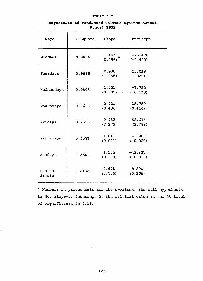
Table 6.5
Regression of P r e d i c t e d Volumes against A c t u a l A u g u s t 1992
Days
Monday S
Tuesday S
Wednesdays
Thursdays
Fridays
Saturdays
Sundays
Pooled Sample
R-Square Slope Intercept
* Numbers in parenthesis are the t-values. The null hypothesis is Ho: slope=l, intercept=O. The critical value at the 5% level
of significance is 2.13.

a The perfect prediction line
@ The model prediction line
Predicted
Actual
Fig. 6.2: The Regression Line of Predicted
Volumes against Actual Volumes

a probability distribution function to be estimated. More importantly,
it has a distinct advantage of constructing and estimating a preference
density function which can be used with any new set of prices and
products. Thus the introduction of new goods on the implication of
different price structure can easily be investigated.
The preference recovery technique presented in this chapter, in
fact in the entire thesis, is not without limitations. First, the
maximum likelihood approach employed assumes a unimodal distribution of
aggregate preferences in (U, v) parameter space. Should data give rise
to a multimodal distribution of preference (for instance, the
population is composed of distinct groups) , the proposed empirical
estimation procedure will not be appropriate. Secondly, as a limitation
to all other discrete choice models, data is a major source of
constraint. As a result, the estimation procedure inevitably involves
some ad hoc restrictions.
The thesis can be extended along the following lines: first, to
compare our method of preferences recovery with other appropriate
discrete choice models with a given data set; second, to develop other
preference recovery techniques, such as nonparametric smoothing
techniques to estimate address models of product differentiation;
finally, to relax some of the assumptions made in this thesis to test
the robustness of our results.
The main purpose of thesis was to demonstrate the feasibility
of preference recovery in address models of product differentiation.
While the preference recovery techniques were illustrated within
particular applications, they should be considered general techniques

that can be applied to other cases of product differentiation.

REFERENCES
Allais, M.(1953), "Le comportement de llhomme rationnel devant le risque: critique des postulats et axiomes de l'ecole Americaine, " Econometrica 21 (4), 503-46.
Allais, M. (1979), "The foundations of a positive theory of choice involving risk and a criticism of the postulates and axioms of the American school,1r In Allais, M. and Hagen, 0. (ed.) Expected U t i l i t y Hypothesis and the A l l a i s Paradox, Reidel, Dordrecht, Holland.
Allais, M. and Hagen, 0. (1979), Expected U t i l i t y Hypotheses and the A l la i s Paradox, ~eidel, Dordrecht, Holland.
Amemiya, T. (1 9 8l), llQualitative Response Models: A Survey. Journal o f Economic Literature 19, 1483-1536.
Anderson, S. P. and de Palma, A.(1988), "Spatial Price Discrimination with Heterogeneous ProductsIg1 Review o f Economic Studies 55, 573-592.
Anderson, S. P., de Palma, A. and Thisse, J. -F. (1989a), "Demand for Differentiated Products, Discrete Choice Models, and the Characteristics Approach," Review o f Economic Studies 56, 21-35.
Anderson, S. P., de Palma, A. and Thisse, J. -F. (l992), Discrete Choice Theory o f Product Di f f eren t ia t ion , Cambridge : MIT Press.
Archibald, G.C. and Eaton, B.C. (19891, "Two Applications of Characteristics Theory. m in G. R. Feiwel (ed. ) , The Economics o f Imperfect competition and Employment : Joan Robinson and Beyond. London: Macmillan, 387-406.
Archibald, G. C., Eaton, B.C. and Lipsey, R.G. (1986), "Address Models of Value," In J. E. Stiglitz and F. G. Mathewson (eds.), New Developments i n the Analysis o f Market Structure. Cambridge: MIT Press, 3-47.
Arrow, K. 5. (1959), "Rational Choice Functions and Orderings." Economica 26, 121-127.
Aumann, R. (1977), "The St. Petersburg Paradox: A Discussion of Some Resent Comments," Journal o f Economic Theory 14 (2), 443-45.
Battalio, R., Kagel, J., and Jiranyakul, R. (l990), "Testing

Between ~lternative Models of Choice under Uncertainty: Some Initial Results, " Journal of Risk and Uncertainty 3 (l), 25-50.
Berkson, J. (lgsl), Why I Prefer Logits to Probits. ~iometrics 7, 327-339.
Berry, S. T.(1992), "Estimating Discrete Choice Models of Product Differentiation," Working Paper, Yale University and NBER.
Brown, J.N. and Rosen, H.S. (1982), "On the Estimation of Structural Hedonic Price Models," Econometrica 46, 149-158.
Burton, Peter S. (1992), "The Use of Product Choice to Reveal the Distribution of Expenditures across Preference Types," Working Paper No. 92-05, Department of Economics, Dalhousie University.
Camerer, C.(1989), "An Experimental Test of Several Generalized Utility Theories, " Journal of Risk and Uncertainty 2 (l), 61-104.
Camerer, C. (1991) , "Resent Tests of Generalized Utility Theories, in Edwards, W. (ed. ) , Utility: Measurement, Theory and Applications, Kluwer, Nijhoff, Amsterdam, XX.
Chamberlin, E. (1933), The Theory of Monopolistic Competition. Cambridge: Harvard University Press.
Chew, S. (l983), "A Generalization of the Quasilinear Mean with Applications to the Measurement of Income Inequality and Decision Theory Resolving the Allais Paradox, Econometrica 51 (4), 1065-92.
Chew, S.
Chew, S.
Chew, S.
Chew, S.
(1985), "Implicit-Weighted Utility Theories, M-estimators, and Non-demand Revelation of Second-price Auctions for an Uncertain Auctioned Object," Johns Hopkins University Department of Political Economy working paper #155.
(1989) , "An Axiomatic Generalization of the Quasilinear Mean and Gini Mean with Application to Decision Theory," Unpublished paper, Johns Hopkins University.
and Epstein, L. (1989), "A Unifying Approach to Axiomatic Non-Expected utility Theories, Journal of Economic Theory, 46 (l), 186-193.
and MacCrimmon, K. (1979), "Alpha-nu Choice Theory: An Axiomatization of Expected Utility." University of British ~olumbia Faculty of Commerce working paper #669.

Chew, S. and Waller, W. S. (1986), "Empirical Tests of Weighted Utility Theory, " Journal o f Mathematical Psychology, 30, .SS-72.
Coombs, C. and Huang, L. (19761, "Tests of the Betweeenness Property of Expected utility, " Journal o f ~ a t h e m a t i c a l Psychology 13, 323-337.
Dekel, E. (1986), "An Axiomatic Characterization of Preferences under Uncertainty: Weakening the Independence Axiom, " Journal o f Economic Theory 40, 304-318.
Dixit, A., and Stiglitz, J. E.(1977), "Monopolistic Competition and Optimum Product Diversity, " American Economic R e v i e w 67, 297-308.
Dixit, A., and Stiglitz, J. E. (1979), "Monopolistic Competition and Optimum Product ~iversity: Reply." American Economic R e v i e w 69, 961-963.
Eaton, B. C. (1972) , "Spatial Competition Revisited. " Canadian Journal o f Economics 5 , 268-278.
Eaton, B. C., and Lipsey, R. G. (1975), "The Principle of Minimum Differentiation Reconsidered: Some New Developments in the Theory of Spatial Competition," Review o f Economic S t u d i e s 42, 27-49.
Eaton, B. C., and Lipsey, R. G. (19771, "The Introduction of Space into the Neo-classical Model of Value Theory," In M. J. Arts and A. R. Nobay (eds. ) , S t u d i e s i n Modern Economic Ana ly s i s . Oxford: ~asil Blackwell, 59-96.
Eaton, B. C., and Lipsey, R. G. (l978), "Freedom of Entry and the Existence of Pure Profits," Economic Journal 88, 455-469.
Eaton, B. C., and Lipsey, R. G. (19891, "Product Differentiation." In R. Schmalensee and R. D. Willig (eds.), Handbook o f I n d u s t r i a l Organizat ion, Vol. 1. Amsterdam: North-Holland, 723-763.
Eaton, B. C., and Wooders, M. H. (1985), "Sophisticated Entry in a Model of Spatial CompetitionItl Rand Journal o f Economics 16, 282-297.
Ellsberg, D. (1961), "Risk, Ambiguity and the Savage Axioms," Q u a r t e r l y Journal o f Economics 75 (4), 643-69.
Fishburn, P. (1978), "On Handars 'new Theory of Cardinal Utilityt and the Maximization of Expected Return," Journal o f P o l i t i c a l Economy 86 (21, 321-4.

Fishburn, P. (1982), The Foundations o f Expected U t i l i t y , Reidel, Dordrecht, Holland.
Fishburn, P. C., and Falmagne, J. -C.(1989), "Binary Choice Probabilities and Rankings," Economics Le t ters 31, 113-117.
Feenstra, R.C. and ~evinsohn, J. A. (l989), "Estimating Demand and Oligopoly Pricing for Differentiation Products with Multiple Characteristics," Working Paper, Institute for International Economic Studies, S-106, 91, Stockholm, Sweden.
Friedman, M. and Savage, L. J. (19481, "The Utility Analysis of Choices Involving Risk, " Journal o f Po l i t i ca l Economy 56 (4), 279-304.
Harless, D. W. (1987), "~redictions About Indifference Curves in the Unit Probability Triangle: A test of Some Competing Decision Theories," Mimeograph, 1ndiana University.
Harris, R. (1984), "Applied General Equilibrium Analysis of Small Open ~conomies with Scale Economies and Imperfect Competition, " The American Economic Review 74 (5 ) , 1016-1032.
Hausman, J. A., and McFadden, D. (1984), "Specification Tests for the Multinomial Logit Model, " Econometrica 52, 1219-1240.
Hausman, J., and Wise, D. A. (1978, "A Conditional Probit Model for Qualitative Choice: Discrete Decisions Recognizing Interdependence and Heterogeneous Preferences, Econometrica 46, 403-426.
Hotelling, H.(1929), "Stability in Competition", Economic Journal 39, 41-57.
Kahneman, D. and Tversky, A. (1979), "Prospect Theory: An Analysis of Decision under Risk," ~conometrica 47(2), 263-91.
Kamakura, W. A., and Srivastava, R. K. (19861, "An Ideal-Point Probabilistic Choice Model for Heterogeneous Preferences," Marketing Science 5, 199-218.
Karmarkar, U. (1978), "Subjectively weighted utility: A ~escriptive Extension of the Expected utility Model," Organizational ~ e h a v i o r and Human Performance 21 (l), 61-72.
Karmarkar, U. (1979), "Subjectively Weighted Utility and the

Allais Paradox, " Organizat ional Behavior and Human Performance 24 (l), 67-72.
Karni, E., and Saf rat Z. (1987), "Preference Reversal and the Observability of Preferences by Experimental Methods," Econometrica 55 (31, 675-85.
Knight, F. (1921) , Risk , Uncer ta in t y and P r o f i t , Houghton Mifflin, New York.
Lancaster, K. J. (1966), "A New Approach to Consumer Theory," Journal o f P o l i t i c a l Economy 74, 132-157.
Lancaster, K. J. (1971), Consumer Demand: A New Approach. New York: Columbia university Press.
Lancaster, K. J. (1979), V a r i e t y , Equ i t y and E f f i c i e n c y . New York: Columbia University Press.
Loomes, G. and Sugden, R. (1982), "Regret Theory and Measurable Utility Theory," Economics L e t t e r s 12, 19-22.
Luce, R. (1991), "Rank- and Sign-dependent Linear Utility Models for Binary Gambles," Journal o f Economic Theory 53(1), 75-100.
MacCrimmon K. (1968), "Descriptive and Normative Implications of the Decision Theory Postulates," In Borch, K.H. and Mossin, J. Risk and Uncer ta in t y : Proceedings of a Conference Held by the International Economic Association.
MacCrimmon, K. and Larsson, S. (1979), "Utility Theory: Axioms versus Paradoxes, in Allais, M. and Hagen, 0. (ed.), Expected U t i l i t y Hypotheses and the ~ l l a i s Paradox, Reidel, Dordrecht, Holland.
Machina, M. (1982), "Expected Utilityf Analysis without the Independence Axiom, ~ c o n o m e t r i c a 50 ( 2 ) , 277-323.
Machina, M. (1983a) , "The Economic Theory of Individual Behavior toward Risk: Theory, Evidence and New Directions, 'l Technical Report No.433, Centre for Research on Organizational Efficiency, Stanford.
Machina, M. (1983b), "Generalized Expected Utility Analysis and the Nature of Observed Violations of the Independence Axiom," in Stigum, B., and Wenstop, F. (ed.), Foundations o f U t i l i t y and Risk w i t h App l i ca t i ons , Reidel, Dordrecht, Holland.
Machina, M. (1987), "Choice under Uncertainty: Problems Solved and Unsolved, Journal o f Economic P e r s p e c t i v e s 1 (1) ,

Machina, M. (1 989) , "Dynamic Consistency and Non-expected Utility Models of Choice under Uncertainty," Journal o f Economic L i t e r a t u r e 27 (4), 1622-1688.
Machina, M. J. (1985), "Stochastic Choice Functions Generated from ete er minis tic Preferences over ~otteries, Economic Journal 95, 575-594.
Manski, C. F. (19771, "The Structure of Random Utility Models," Theory and Decis ion 8, 229-254.
Manski, C. F., and McFadden, D. (eds.), (1981), S t r u c t u r a l A n a l y s i s o f d i s c r e t e Data wi th Econometric A p p l i c a t i o n s . Cambridge: MIT Press.
Marschak, J. (1950), "Rational Behavior, Uncertain Prospects and Measurable utility," Econometrica 18, 111-141.
MacCrimmon, K.R. and Larsson, S. (1979), "Utility Theory: Axioms Versus Paradoxes," In Maurice Allais and Hagen, O.(eds). The Expected U t i l i t y Hypothesis and A l l a i s Paradox. Dordrecht: D. Reidel Publishing Co.
Marshall,
McFadden,
McFadden,
McFadden,
McFadden,
McFadden,
McFadden,
R.C., Richard, J. and Zarkin, G.A. (1992), "Posterior Probabilities of the Independence Axiom With Nonexperimental Data (or Buckle Up and Fan Out)," Journal o f Bus iness & Economic S t a t i s t i c s 10 (l), 31-44.
D. (1974), "Conditional Logit Analysis of Qualitative Choice Behavior," In P. Zaremka (ed.) , F r o n t i e r s i n Econometrics. New York: Academic Press, 105-142.
D. (1976), "Quantal Choice Analysis: A Survey." Annals o f Economic and Soc ia l Measurement 5/6, 363-390.
D. (1980), "Econometric Models of Probabilistic Choice among ProductsI1' Journal o f Bus iness 53, 513-529.
D. (1981), "Econometric Models of Probabilistic Choice," In C. F. Manski and D. McFadden (eds. ) , S t r u c t u r a l A n a l y s i s o f D i sc re t e Data wi th Econometric App l i ca t i ons . Cambridge: MIT Press, 198-272.
D. (1984) , "Econometric Analysis of Qualitative Response model^,'^ In Z. Griliches and M. D. Intriligator (eds . ) , Handbook o f Econometrics. Volume 2. Amsterdam: North-Holland, 1395-1457.
D. (1986), "The Choice Theory of Market Research," Marketing Sc i ence 5 , 275-297.

McFadden,
Morrison,
Neven, D.
D., and Richter, M. K. (1990), "Stochastic Rationality and Revealed Stochastic Preference," In J. S. Chiman, D. McFadden, and M. K. Richter (eds.) , Preference, uncertainty, and ~ptimality. Essays in Honor of Leonid ~urwicz. Boulder: westview Press, 161-186.
D.G (1967), "On the Consistency of Preferences in Allais Paradox", Behavioral Science 12, 373-83.
(1986), "Address' Models of Differentiation, In G. Norman (eds. 1, Spatial Pricing and Differentiated Markets. London:Pion, 5-18.
Norman, G. (1983), "Spatial pricing with Differentiated Products,"
Quarterly Journal of Economics 97, 291- 310.
oum, T. H. (1979), "A Warning of the Use of in ear Logit ~odels in Transport Mode Choice Studies," Bell Journal of Economics 10, 374-388.
Penny, K. Goldberg, (1992), "Product Differentiation and Oligopoly in International Markets: The Case of the U.S. Automobile Industry, " Working Paper, Princeton University.
Perloff, J. M., and Salop, S. C.(1985), "Equilibrium with Product Differentiation, Review of Economic Studies 52, 107-120.
Quandt, R. E. (1956), "A ~robabilistic Theory of Consumer
Behavior, " Quarterly Journal of ~conomics 70, 507-536.
Quiggin, J. (l982), "A Theory of Anticipated Utility," Journal of Economic Behavior and Organization 3 (4), 323-43.
Quiggin, J. (1985), "Anticipated Utility, Subjectively Weighted Utility and the Allais Paradox," Organizational Behavior and Human Performance 35 (1 ) , 94-101.
Quiggin, J. (1 992) , The Rank-Dependent Expected Utility Model, Unpublished book, University of Maryland and Australian National University.
Ramsey, F.P. (1931), "Truth and Probability," In Braithwaith R.B. (eds), The Foundations of Mathematics and Other Logical Essays, New York: Humanities Press, 1950.
Rosen, H.S. (19741, "Hedonic Prices and Implicit Markets: Product Differentiation in Pure Competition," Journal of

Political Economy 82, 34-55.
Rothschild, M. and Stiglitz, J. (19701, "Increasing Risk: I. A Definition, Journal of E C O ~ O ~ ~ C Theory 2 (4), 225-243,
~othschild, M. and Stiglitz, J. (l97l), "Increasing Risk: 11. Its A Economic Consequences, Journal of Economic Theory 3 (l), 66-84.
Schoemaker, P. (1982), "The Expected Utility Model: Its Variants, Purposes, Evidence and Limitations," Journal of Economic Literature 20, 529-563.
Segal, U. (1989), "Anticipated Utility: A measure Representation Approach," Annals of Operations Research 19, 359-74.
Slovic, P. and Lichtenstein, S., (1968), "The Relative Importance of Probabilities and Payoff S in Risk taking, Journal of Experimental Psycho1 ogy 78, 1-1 8.
Slovic, P. and Tversky, A. (19741, "Who Accept Savage's Axiom?", Behavioral Science 19, 368-373.
Starmer, C., and Sugden, R. (1987a), "Experimental Evidence of the Impact of Regret on Choice Under Uncertainty," Economic Research Centre discussion paper no. 23, University of East Anglia.
Starmer, C., and Sugden, R. (1987b1, "Violations of the Independence Axiom: An Experimental Test of Some Competing Hypothesis," Economic Research Centre discussion paper no. 24, University of East Anglia.
Train, K. (1986) , Qualitative Choice Analysis: Theory, Econometrics, and an Application to Automobile Demand. Cambridge: MIT Press.
Tversky, A. (1969), "Intransitivity of Review 76, 31-48.
von Neumann, J. and Morgenstern, 0.
Economic Behavior, Princeton
Preferences, " Psych01 ogical
1944 ) , Theory of Games and University Press.