preface - faculty personal homepage- kfupmfaculty.kfupm.edu.sa/math/ahasan/coursecontents/chapter...

CONTENTS

PREFACE

1. Introduction to Differential Equations

1.1 Introduction

1.2 Definitions and Terminology

1.3 Initial-Value and Boundary-Value Problems

1.4 Differential Equations as Mathematical Models

1.4.1. Population Dynamics (Logistic Model of Population Growth)

1.4.2. Radioactive Decay and Carbon Dating

1.4.3. Supply, Demand and Compounding of Interest

1.4.4 Newton's law of Cooling/Warming

1.4.5 Spread of a Disease

1.4.6 Chemical Reactions

1.4.7 Chemical Mixtures

1.4.8 Draining a Tank.

1.4.9 Series Circuit

1.4.10 Falling Body

1.4.11 Artificial Kidney

1.4.12 Survivability with AIDS( Acquired immunodeficiency )

1.5 Exercises

2. First-Order Differential Equations

2.1 Separable Variables

2.2 Exact Equations

1

2.2.1 Equations Reducible to Exact Form

2.3 Linear Equations

2.4 Solutions by Substitution

2.4.1 Homogenous Equation.

2.4.2 Bernoulli’s Equation

2.5 Exercises

3. First-Order Differential Equations of Higher Degree.

3.1 Equations of the First-order and not of First Degree

3.2 First-Order Equations of Higher Degree Solvable for Derivative

3.3 Equations Solvable for y

3.4 Equations Solvable for x

3.5 Equations of the First Degree in x and y - Lagrange and Clairant

Equations

3.6 Exercises

4. Applications of First Order Differential Equations to Real World Systems

4.1 Cooling/Warming Law

4.2 Population Growth and Decay

4.3 Radio-Active Decay and Carbon Dating

4.4 Mixture of Two Salt Solutions

4.5 Series Circuits

4.6 Survivability with AIDS

4.7 Draining a tank

4.8 Economics and Finance

2

4.9 Mathematics Police Women

4.10 Drug Distribution in Human Body

4.11 A Pursuit Problem

4.12 Harvesting of Renewable Natural Resources

4.13 Exercises

5. Higher Order Differential Equations

5.1 Initial-value and Boundary-value Problems

5.2 Homogeneous Equations

5.3 Non-homogeneous Equations

5.4 Reduction of order

5.5 Solution of Homogeneous Linear Equations with Constant Coefficients

5.6 The Method of Undetermined Coefficients

5.7 The Method of Variation of Parameters

5.8 Cauchy-Euler Equation

5.9 Non-linear Differential Equations

5.10 Exercises

6. Power Series Solutions of Linear Differential Equations

6.1 Review of Properties of Power Series

6.2 Solutions about Ordinary Points

6.3 Solutions about Regular Singular Points - The Method of Frobenius

6.4 Bessel’s Equations and Functions

6.5 Legendre’s Equations and Polynomials

6.6 Orthogonality of Functions

3

6.7 Sturm – Liouville Theory

6.8 Exercises

7. Modelling and Analysis of Real World Systems by Higher Order

Differential Equations

7.1 Series Electrical circuit

7.2 Falling Bodies

7.3 The shape of a Hanging cable. The power line problem

7.4 Diabetes and glucose Tolerance Test

7.5 Rocket Motion

7.6 Undamped and Damped motion

7.7 Exercises

8. System of Linear Differential Equations with Applications

8.1 System of linear first order Equations

8.2 Matrices and Linear Systems

8.3 Homogeneous Systems : Distinct Real Eigenvalues

8.4 Homogeneous Systems : Complex and Repeated Real Eigenvalues

8.5 Method of Variation of Parameters

8.6 Matrix Exponential

8.7 Applications

8.7.1 Electrical circuits

8.7.2 Coupled springs

8.7.3 Mixture Problems

8.7.4 Arms Race

4

8.8. Exercises

9. Laplace Transforms and Their Applications to Differential Equations

9.1 Definition and Fundamental Properties of The Laplace Transform

9.2 The Inverse Laplace Transform

9.3 Shifting Theorems and Derivative of Laplace Transform

9.4 Transforms of Derivatives, Integrals and Convolution Theorem

9.4.1 The Laplace Transform of Derivatives and Integrals

9.4.2 Convolution

9.4.3 Impulse Function and Dirac Delta Function

9.5 Applications to Differential and Integral Equations

9.6 Exercises

10. Numerical Methods for Ordinary Differential Equations.

10.1 Direction Fields

10.2 Euler Methods

10.3 Runge-Kutta Methods

10.4 Picard's Method of Successive Approximation

10.5 Exercises

11. Introduction to Partial Differential Equations

11.1 Basic concepts and Definitions

11.2 Classification of Partial Differential equations

11.2.1 Initial and Boundary Value Problems

11.2.2 Classification of second order Partial Differential Equations

11.3 Solutions of Partial Differential Equations of First Order

5

11.3.1. Solutions of Partial Differential Equations of First order with

constant coefficients.

11.3.2. Lagrange's Method for Partial Differential Equations of First-order

with Variable coefficients.

11.3.3. Charpit's Method for solving nonlinear Partial Differential

Equations of first-order.

11.3.4. Solutions of Special type of Partial Differential Equations of first

order.

11.3.5. Geometric concepts Related to Partial Differential Equations of

first-order.

11.4 Solutions of Linear Partial Differential Equations of Second order with

constant coefficients.

11.4.1 Homogeneous Equations

11.4.2 Non-homogeneous Equations

11.5 Monge's Method for a special class of nonlinear Equations (Quasi linear

Equations) of the second order.

11.6 Exercises.

12. Partial Differential Equations of Real World Systems

12.1 Partial Differential Equations as Models of Real World Systems

12.2 Elements of Trigonometric Fourier Series for Solutions of Partial

Differential Equations

12.3 Method of Separation of Variables for Solving Partial Differential

Equations

6

12.3.1 The Heat Equation

12.3.2 The Wave Equation

12.3.3 The Laplace Equation

12.4 Solutions of Partial Differential Equations with Boundary conditions

12.4.1 The Wave Equation with Initial and Boundary conditions

12.4.2 The Heat Equation with Initial and Boundary conditions

12.4.3 The Laplace Equation with Initial and Boundary conditions

12.4.4 Black-Scholes Model of Financial Engineering Mathematics

12.5 Exercises

13. Calculus of Variations with Applications.

13.1 Variational problems with fixed boundaries

13.2 Applications to concrete Problems

13.3 Variational Problems with moving boundaries

13.4 Variational Problems involving derivatives of higher order and several

independent variables

13.4.1 Functionals involving several dependent variables.

13.5 Sufficient conditions for an Extremum-Hamilton-Jacobi Equation

13.6 Exercises

Bibliography

Appendices

Solutions/Hints of Selective Exercises

Index.

7

Chapter - I

1. Introduction to Differential Equations

1.1 Introduction



1.4 Differential Equations as Mathematical Models










1.4.10 Falling Body



1.5 Exercises

1.1 Introduction

The words differential and equations clearly indicate solving some

kind of equation involving derivatives. Differential equations are interesting and

important because they express relationships involving rates of change. Such

8

relationships form the basis for developing ideas and studying phenomena in the

sciences, economics, engineering, finance, medicine and in short without any

exaggeration every aspect of human knowledge. We will see examples of

applications to real world problems in Section 1.4 and subsequent chapters.

The study of differential equations originated in the investigation of

laws that govern the physical world and were first solved by Sir Isaac Newton in

seventeenth century (1642-1727) , who referred to them as 'fluxional equations.

The term differential equation was introduced by Gottfried Leibnitz, who was

contemporary of Newton. Both are credited with inventing the calculus. Many of

the techniques for solving differential equations were known to mathematicians of

this century, but a general theory for differential equations was developed by

Augustin-Louis Cauchy (1789-1857). Applications to stock markets and problems

related to finance and legal profession, studied towards the later part of twentieth

century can be found in the work of Myron S. Scholes and Robert C. Merton who

were awarded Nobel Prize of Economics in 1997. The three aspects of the study

of differential equations - theory, methodology and application - are treated in this

book with the emphasis on methodology and application. The purpose of this

chapter is two-fold: to introduce the basic terminology of differential equations

and to examine how differential equations arise in endeavour to describe or

model physical phenomena or real world problems in mathematical terms.


Definition 1.2.1 Differential Equation

9

An equation containing the derivatives of one or more dependent

variable, with respect to one or more independent variables, is said to be a

differential equation (DE).

Definition 1.2.2 Ordinary Differential Equation

A differential equation is said to be an ordinary differential equation

(ODE) if it contains only ordinary derivatives of one or more dependent variables

with respect to a single independent variable.

Definition 1.2.3 Partial Differential Equation

An equation involving the partial derivatives of one or more

dependent variables of two or more independent variables is called a partial

differential equation (PDE).

10

Example 1.

are examples of ordinary differential equation.

Example 2.

are examples of partial differential equation.

Definition 1.2.4 Order of a Differential Equation

The order of a differential equation (ODE or PDE) is the order of the

highest derivative in the equation.

Example 3. (i) Order of the differential equation

(ii) Order of the differential equation

is 3

Definition 1.2.5 Degree of a Differential Equation

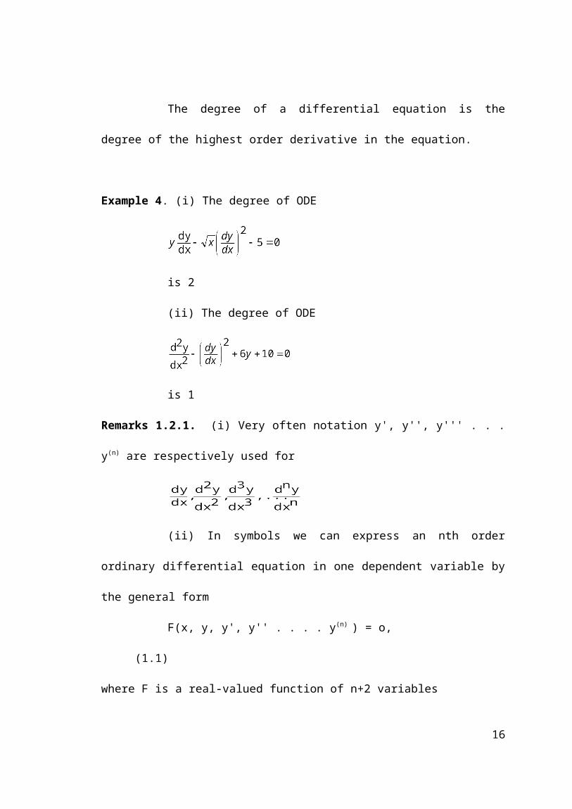
The degree of a differential equation is the degree of the highest

order derivative in the equation.

Example 4. (i) The degree of ODE

11

is 2

(ii) The degree of ODE

is 1

Remarks 1.2.1. (i) Very often notation y', y'', y''' . . . y(n) are respectively used for

(ii) In symbols we can express an nth order ordinary differential

equation in one dependent variable by the general form

F(x, y, y', y'' . . . . y(n) ) = o, (1.1)

where F is a real-valued function of n+2 variables

x, y, y’, y” y”’ ... . . . y

(n)

and where y(n)

=

Definition 1.2.6 Linear and Non-linear Differential Equations

An nth-order ordinary differential equation is said to be linear in y if

it can be written in the form

an(x)y(n)+an-1(x)y(n-1) + . . . . . + a1(x)y’+ao(x)y = f(x)

where ao, a1, a2 . . ., an and f are functions of x on some interval, and

an(x) 0 on that interval. The functions ak(x), k=0, 1, 2, . .. . , n are called the

coefficient functions. A differential equation that is not linear is called non-linear.

Example 1.5

12

(i) y''=4y'+3y=x4 and

xy''+yex+6=0 are linear differential equations.

(ii)

y’‘-4y’+y=0 are linear differential equations.

(iii)

are non-linear.

Remark. 1.2.2 An ordinary differential equation is linear if the following

conditions are satisfied.

(i) The unknown function and its derivatives occur in the first degree

only.

(ii) There are no products involving either the unknown function and

its derivatives or two or more derivates.

(iii) There are no transcendental functions involving the unknown

function or any of its derivatives.

Definition 1.2.7 Solutions:

(i) A solution or a general solution of an nth-order differential

equation of the form (1.1) on an interval I = [a,b] = {xR/a xb} is any function

possessing all the necessary derivatives, which when substituted for y, y’,

13

y’’ . . . ., y(n), reduces the differential equation to an identity. In other words an

unknown function is a solution of a differential equation if it satisfies the equation.

(ii) A solution of a differential equation of order n will have n

independent arbitrary constants. Any solution obtained by assigning particular

numerical values to some or all of the arbitrary constants is called a particular

solution.

(iii) A solution of a differential equation that is not obtainable from a

general solution by assigning particular numerical values is called a singular

solution.

(iv) A real function y = (x) is called an explicit solution of the

differential equation F(x,y, y’, . . . , y(n)) = 0 on [a, b] if

F(x, (x), ’(x), . . . , (n) (x) ) = 0 on [a, b].

(v) A relation g(x,y) = 0 is called an implicit solution of the

differential equation F(x, y, y’, . . . , y(n) ) = 0 on [a, b] if g(x, y) = 0 defines at least

one real function f on [a, b] such that y = f(x) is an explicit solution on this interval.

We now illustrate these concepts through the following examples:

Example 1.6 (i) y = c1 ex+c2 is a solution of the equation

y’’-y=0

This ODE is of order 2 and so its solution involves 2 arbitrary

constants c1 and c2. It is clear that

y’ = c1 ex+c2, y’’ = c1 ex+c

2 and so c1 ex+c2 - c1 ex+c

2 = 0.

Hence y=c1 ex+c2 is a general solution or simply a solution.

(ii) y = ce2x is a solution of ODE y’-2y = 0,

14

because y’ =2ce2x and y=ce2x satisfy the ODE. Since given

ODE is of order 1, solution contains only one constant.

(iii) y=cx+ c2 is a solution of the equation

(y’)2 + xy’ – y = 0

To verify the validity, we note that y’=c, and therefore

(c)2+cx-(cx+ c2)=0

(iv) y=c1 e2x+c2e-x is a general solution of the differential equation

y’’=y’-2y=0 of order 2.

To check the validity we compute y’ and y’’ and put values in these

equation.

y’ = 2c1e2x - c2e-x, y’’=4c1 e2x+c2e-x

L.H.S. of the given ODE is = (4c1 e2x+c2e-x)-(2c1e2x-c2e-x)

-2(c1e2x+c2e-x)

= 0

Example 1.7 (i) Choosing c=1 we get a particular solution of differential equation

considered in Example 1.6(iii).

(ii) For c1 = 1 we get a particular solution of differential equation in

Example 1.6(i) that is, y=ex+c2 is a particular solution of y''-y=0.

Example 1.8 (i) y = - x2 is a singular solution of differential equation in Example

1.6(iii) .

15

y = - x2 is not obtainable from the general solution y=cx+ c2.

However, it is a solution of the given differential equation, can be checked as

follows:

y’ =-x. By putting values of y and y ’ into the RHS of the equation we get

(-x)2+x(-x)-(- x2) = x2-x2 =0

(ii) y = 0 is a singular solution of y’ = xy1/2

Verification: The general solution of this equation is y = +c. For c=0, we do

not get the solution y=0. Therefore, the solution y=0 of the equation is not

obtainable from the general solution.

Hence y=0 is a singular solution.

Example 1.9. (i) y = sin 4x is an explicit solution of y’’+16y=0 for all real x.

Verification: y’=-4 cos 4x, y’’=-16 sin 4x. Putting the value of y and y’’ in terms of

x into the RHS of equation we get –16 sin 4x+16 sin 4x=0.

Hence equation is satisfied for y = sin 4x.

Therefore y=sin4x is an explicit solution of the given equation.

(ii) y=c1 ex+c2e-x is an explicit solution of the equation y’’-y=0

Verification: y’ = c1ex –c2e-x, y’’ = c1 ex+ c2e-x. Put values of y and y’’ in the RHS of

the given equation to get (c1ex+c2e-x) - (c1ex+c2e-x)

= 0.

Example 1.10 : (i) The relation x2+y2 = 4 is an implicit solution of the differential

equation

on the interval (-2,2).

16

Verification: By implicit differentiation of the relation x2+y2=4 we get

or

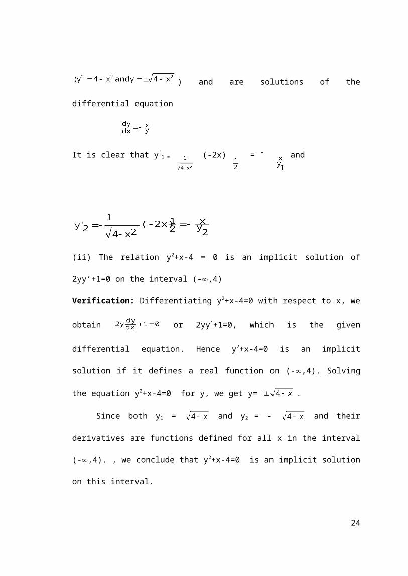
Further, y1 = satisfying the relation

) and are solutions of the differential equation

It is clear that y’1 = (-2x) = -

and

(ii) The relation y2+x-4 = 0 is an implicit solution of 2yy’+1=0 on the interval (-,4)

Verification: Differentiating y2+x-4=0 with respect to x, we obtain or

2yy’+1=0, which is the given differential equation. Hence y2+x-4=0 is an implicit

solution if it defines a real function on (-,4). Solving the equation y2+x-4=0 for y,

we get y= .

Since both y1 = and y2 = - and their derivatives are functions

defined for all x in the interval (-,4). , we conclude that y2+x-4=0 is an implicit

solution on this interval.

Remark 1.2.3 It is very pertinent to note that a relation g(x,y) = 0 can reduce a

differential to an identity without constituting an implicit solution of the differential

equation. For example x2+y2+1 = 0 satisfies yy’+x=0, but it is not an implicit

17

solution as it does not define a real-valued function. This is clear from the

solution of the equation x2+y2+1 = 0 or y=1-x2, imaginary number.

The relation x2+y2+1 = 0 is called a formal solution of yy’+x=0. That

is it appears to be a solution. Very often we look for a formal solution rather than

an implicit solution.

Differential Equation of a Family of Curves

Let us consider an equation containing n arbitrary constants. Then

by differentiating it successively n times we get n more equations containing n

arbitrary constants and derivatives. Now by eliminating n arbitrary constants from

the above (n+1) equations and obtaining an equation which involves derivatives

upto the nth order, we get a differential equation of order n. The concept of

obtaining differential equations from a family of curves is illustrated in following

examples.

Example 1.11 Find the differential equation of the family curves

y = ce2x

Solution: Given y = ce2x (1.2)

Differentiating equation (1.2) we get

y’ = 2ce2x = 2 y

or

y’ - 2y = 0 (1.3)

Thus, arbitrary constant c is eliminated and equation (1.3) is the

required equation of the family of curves given by equation (1.2).

18

Example 1.12. Find the differential equation of the family of curves

y = c1 cosx + c2 sin x (1.4)

Solution: Differentiating (1.4) twice we get

y’ = -c1 sin x + c2 cos x (1.5)

y’’ = -c1cos x - c2 sin x (1.6)

c1 and c2 can be eliminated from (1.4) and (1.6) and we obtain the

different equation

y’’ + y = 0 (1.7)

(1.7) is the differential equation of the family of curves given by (1.4).


A general solution of an nth order ordinary differential equation

contains n arbitrary constants. To obtain a particular solution, we are required to

specify n conditions on solution function and its derivatives and thereby expect to

find values of n arbitrary constants. There are two well known methods for

specifying auxiliary conditions. One is called initial conditions and other is said to

be boundary conditions.

It may be observed that an ordinary differential equation does not

have solution or unique solution. However, by imposing initial and boundary

conditions uniqueness can be ensured for certain classes of differential

equations.

19

Definition 1.3.1. initial-Value Problem

If the auxiliary conditions for a given differential equation relate to a

single x value, the conditions are called initial conditions. The differential

equation with its initial conditions is called an initial-value problem.

Definition 1.3.2. If the auxiliary conditions for a given differential equation relate

to two or more x values, the conditions are called boundary conditions or

boundary values. The differential equation with its boundary conditions is called

boundary-value problem.

Example 1.13 (i) y'+y=3, y(0) = 2 is a first-order initial value problem. Order of

initial value problem is nothing but order of the given equation. y(0)=2 is an initial

condition.

(ii) y’’+2y=0, y(1) = 2, y’(1) = -3 is a second-order initial value

problem. Initial conditions are y(1)=2 and y ’(1) =-3. Values of function y(x) and its

derivative are specified for value x=1.

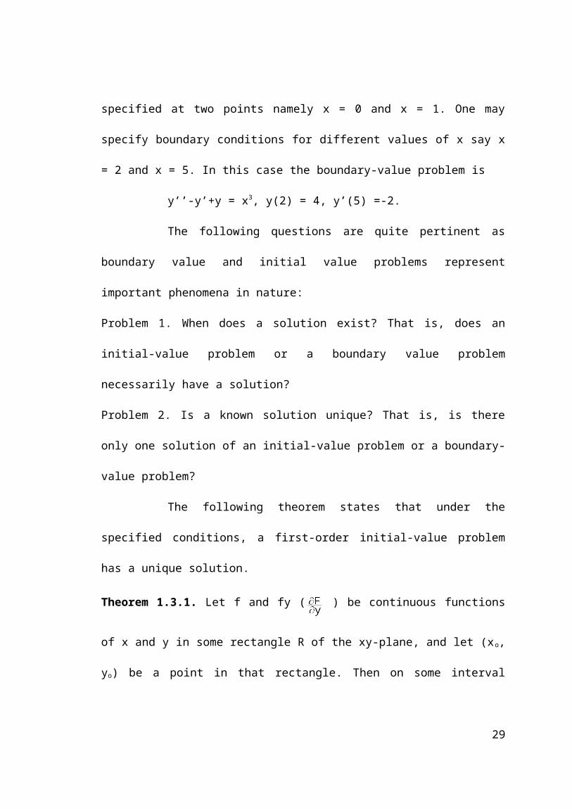
(iii) y’’-y’+y = x3, y(0) = 4, y’(1) =-2 is a second-order boundary-

value problem. Boundary conditions are specified at two points namely x = 0 and

x = 1. One may specify boundary conditions for different values of x say x = 2

and x = 5. In this case the boundary-value problem is

y’’-y’+y = x3, y(2) = 4, y’(5) =-2.

The following questions are quite pertinent as boundary value and

initial value problems represent important phenomena in nature:

Problem 1. When does a solution exist? That is, does an initial-value problem or

a boundary value problem necessarily have a solution?

20

Problem 2. Is a known solution unique? That is, is there only one solution of an

initial-value problem or a boundary-value problem?

The following theorem states that under the specified conditions, a

first-order initial-value problem has a unique solution.

Theorem 1.3.1. Let f and fy ( ) be continuous functions of x and y in some

rectangle R of the xy-plane, and let (xo, yo) be a point in that rectangle. Then on

some interval centred at xo there is a unique solution y = (x) of the initial value

problem:

Figure 1.1 Geometrical Illustration of Theorem 1.3.1.

Example 1.14. (i) y = 3 ex is a solution of the initial-value problem.

y’ = y, y(0) = 3

This means that the solution of the differential equation y ’=y passes

through the point (0,3).

Verification: Let y = cex, where c is an arbitrary constant. Then y ’ = cex = y. Thus,

y = cex is a general solution of the given equation y’=y.

21

By applying initial condition we get 3=y(0) = c eo = c or c = 3.

Therefore y=3ex is a solution of the given initial value problem.

(ii) Find a solution of the initial-value problem y’=y, y(1)=-2. That is,

find a solution of differential equation y’=y which passes through the point (1, -2).

Solution: As seen in part (i) y = cex is a solution of the given equation. By

imposing given initial condition we get

-2=y(1) = c e1 or c = -2/e. Therefore

= -2ex-1 is a solution of the initial-value problem.

Example 1.15

has at least two solutions, namely y=0 and y = x4/16.

Example 1.16 (i) Does a solution of the boundary value problem y’’+y=0, y(0)=0,

y() = 2 exist?

(ii) Show that the boundary value problem

y’’+y=0, y(0) =0, y() = 0 has

infinitely many solutions.

Solution (i) y=c1 cos x+c2 sin x is a solution of the differential equation y’’+y=0.

Using given boundary conditions in y=c1 cos x+c2 sin x, we get

0=c1 coso+c2 sin 0

and

2=c1 cos +c2sin

The first equation yields c1=0 and the second yields c1 =-2 which is absurd,

hence no solution exists.

(ii) The boundary values yield

22

0=c1 cos 0+c2 sin 0

and

0=c1 cos + c2 sin

Both of these equations lead to the fact that c1=0. The constant c2 is

not assigned a value and therefore takes arbitrary values. Thus there

are infinitely many solutions represented by y=c2 sin x.

Example 1.17. Examine existence and uniqueness of a solution of the following

initial-value problems:

(i) y'=y/x,y(2) = 1

(ii) y'=y/x,y(0) = 3

(i) y'= -x,y(0) = 2

Solution (ii) We examine whether conditions of theorem 1.3.1 are satisfied . To

check, we observe that

Both functions are continuous except at x =0.

Hence f and satisfy the conditions of the theorem in any rectangle R

that does not contain any part of the y -axis (x=0). Since the point (2,1)

is not on the y-axis, there is a unique solution. One can check that y=

x is the only solution.

(ii) In this problem neither f nor in continuous at x=0, which means

that (0,3) cannot be included in any rectangle R where f and are

continuous.

23

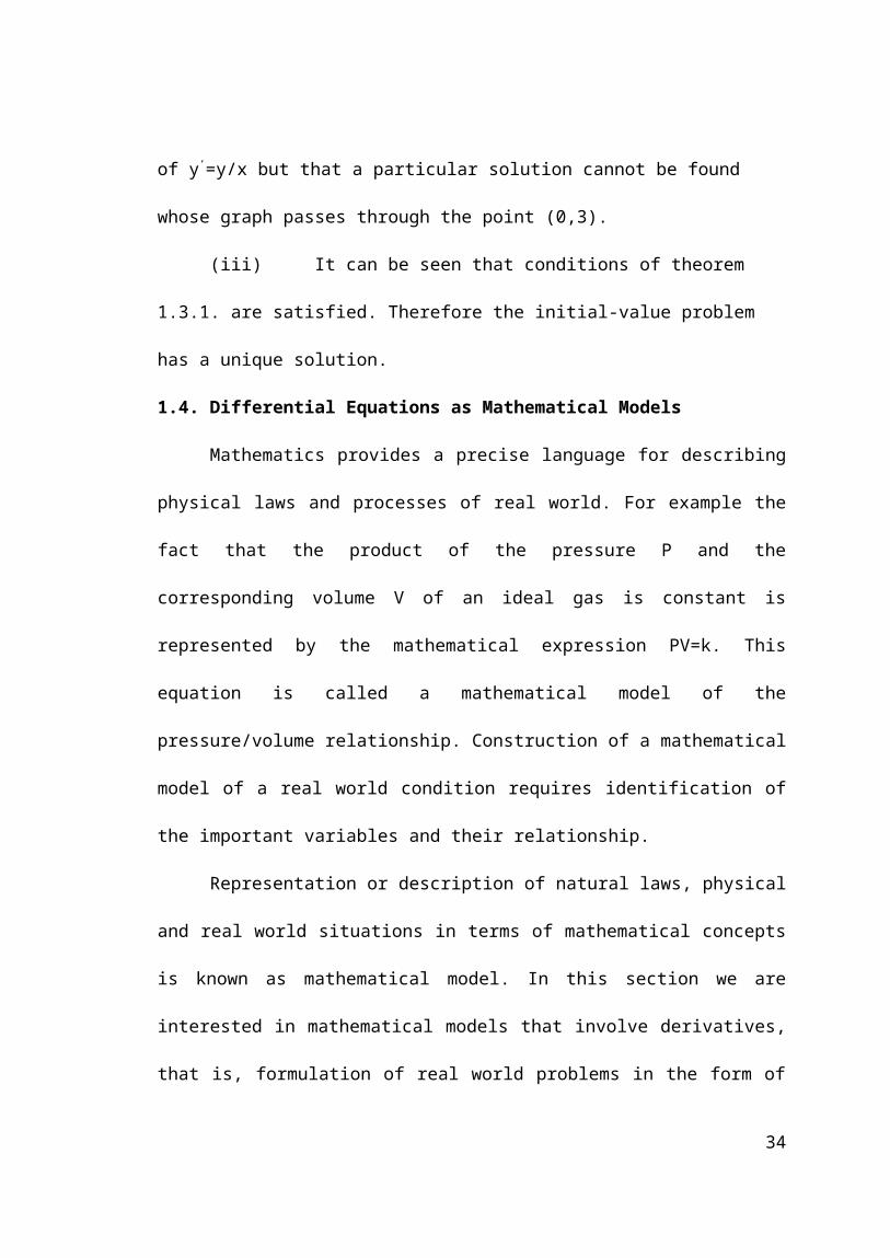
Hence we cannot conclude any thing from theorem 1.3.1. However it can

be verified that y=cx is a general solution of y’=y/x but that a particular solution

cannot be found whose graph passes through the point (0,3).

(iii) It can be seen that conditions of theorem 1.3.1. are satisfied.

Therefore the initial-value problem has a unique solution.

1.4. Differential Equations as Mathematical Models

Mathematics provides a precise language for describing physical laws and

processes of real world. For example the fact that the product of the pressure P

and the corresponding volume V of an ideal gas is constant is represented by the

mathematical expression PV=k. This equation is called a mathematical model of

the pressure/volume relationship. Construction of a mathematical model of a real

world condition requires identification of the important variables and their

relationship.

Representation or description of natural laws, physical and real world

situations in terms of mathematical concepts is known as mathematical model. In

this section we are interested in mathematical models that involve derivatives,

that is, formulation of real world problems in the form of ordinary differential

equations. Modeling of real world problems through partial differential equations

will be treated in chapter 10. We concentrate here on Growth and decay

problems (Radioactive Decay and Carbon Dating, Logistic Model of Population

Growth) Supply and Demand and compounding of interest, Newton’s Law of

Cooling/Warming, Spread of disease, Chemical Reactions, Mixtures, Draining a

Tank, Series Circuits, Falling Bodies, Artificial Kidney, and Aids. We derive

24

models under appropriate assumptions and their solutions will be discussed in

subsequent chapters.

The steps of the modeling process are described in Figure 1.2

Figure 1.2

A model is reasonable if its solution is consistent with either experimental

data or known facts about the physical phenomena or situations. if the

predictions produced by the solution are poor or vague or insufficient, appropriate

modification of the model is carried out by either increasing the level of resolution

of the model or by making alternative assumptions about the mechanisms for

change in the system. A mathematical model of a physical system or

phenomenon will often involve the variable time t. A solution of the model then

gives the state of the system; in other words, for appropriate value of t the values

of the dependent variable (or variables) describe the system in the past, present,

and future.

25


One of the earliest attempts to model human population growth by means

of mathematics was by the English economist Thomas Malthus in 1798.

Essentially, the idea of the Malthusian model is the assumption that the rate at

which a population of a country grows at a certain time is proportional to the total

population of the country at that time. In mathematical terms, if N(t) denotes the

total population at time t, then this assumption can be expressed as

where k is constant of proportionality

Solution of equation (1.8) will provide population at any future time t. This

simple model which does not take many factors into account (immigration and

emigration, for example) that can influence human populations to either grow or

decline, nevertheless turned out to be fairly accurate in predicting the population

of the United States during the years 1790-1860. Populations that grow at a rate

described by (1.8) are rare, nevertheless, (1.8) is still used to model growth of

small populations over short intervals of time, for example, bacteria growing in a

petri dish. In 1837 the Dutch biologist Verhulst improved Malthusian model while

looking at fish population in the Adriatic sea. He reasoned that the rate of change

of population N(t) with respect to t should be influenced by growth factors such

as population itself, and also factors tending to retard the population, such as

limitations on food and space. He constructed a model by assuming that growth

factors could be incorporated into a term a N(t), and retarding factors into a term

26

–bN(t)2, with a and b positive constants whose values depend on the particular

population. From this he obtained the logistic model of population growth:

If we assume initial population (at a time designated as zero) N(0)=No. This

is an initial condition), we will see in chapter .............that the solution of the initial-

value problem

N(o) = No

is

Formula (1.9a) can provide prediction of population after specified years of time.


In most cases a mathematical model is only an approximation of the

physical condition being studied. In the beginning of 20 th century E. Ruther ford,

based on experimental results, was able to formulate a model in terms of a

simple differential equation to describe radio active decay relying on the

assumption that rate at which atoms disintegrate is proportional to the number of

atoms N present in the material.

Let m(t) be the mass of a radioactive substance at time t, then for some

constant of proportionality k that depends on the substance,

(1.10)

27

The solution of (1.10) (We solve this equation in the next chapter) is

the basis for an important technique used to estimate the ages of certain

artefacts. Infact, Libby fetched Nobel prize of chemistry is 1960 for his work

related to this model.

Around 1950 the chemist Willard Libby devised a method of using

radioactive carbon as a means of determining the approximate ages of fossils.

The theory of carbon dating is based on the fact that the isotope carbon-14 is

produced in the atmosphere by the action of cosmic radiation on nitrogen. The

ratio of the amount of C-14 to ordinary carbon in the atmosphere appears to be a

constant, and as a consequence the proportionate amount of the isotope present

in all living organisms is the same as that in the atmosphere. When an organism

dies, the absorption of C-14, by either breathing or eating, ceases. Thus by

comparing the proportionate amount of C-14 present, say, in a fossil with the

constant ratio found in the atmosphere (ordinary carbon-C-12) it is possible to

obtain a reasonable estimation of its age. The method is based on the knowledge

that the half-life of the radio active C-14 is approximately 5600 years. Libby's

method has been used to date furniture in Egyptian tombs, to decide Van

Meegeren Art forgeries and to decide the dates of different civilization through

archaeological excavation.

The process of estimating the age of an artefact or fossil is called carbon

dating. See Example 3 of Chapter 4 for procedure to determine age of an

artefact. Radio active dating has also been used to estimate the age of the solar

system and of earth as 45 billion years. It may be recalled that the half-life is a

28

measure of the stability of a radio active substance. It is simply the time it takes

for one half of the atoms in an initial amount m(o)=M to disintegrate, or transmute

into the atoms of another element.


Suppose that a company is planning to launch a new product in the

market and for this it desires to develop a model to describe the behaviour of the

price of the product. A normal assumption could be that the rate of change of the

price of the product with respect to time is directly proportional to the difference in

the demand and the supply of the product. Basically it is assumed that if the

demand exceeds the supply, the price will go up and if the supply excess the

demand, the price will go down. Let P denote the price of the product at any time

t. Then if D is the demand for the product and S is the supply, the derived model

is

= k (D-S) (1.11)

Where k is the constant of proportionality.

Let s(t) be the amount of money accumulated in a saving account after t years

where r is the annual rate of interest compounded continuously.

If h>o denotes an increment in time, then interest obtained in the time

span (t+h)-t is the difference in the amounts accumulated.

s(t+h)-s(t) (1.12)

Since interest is given by (rate) x (time ) x (principal), we can approximate

the interest earned in this same time period by either

rhs(t) or rhs(t+h) (1.13)

29

Intuitively, the quantities in (1.13) are seen to be lower and upper bounds,

respectively for the actual interest given by (1.12), that is,

rhs(t) s(t+h) - s(t) rhs(t+h) (1.14)

Or rs(t) (s(t+h)-s(t))/h rs(t+h) (1.15)

Since we are interested in the case where h is very small, taking limit in

(1.15) as h o we get

or ds/dt = rs (1.16)

(1.16) is a mathematical model of compounding interest. By solving (1.16)

we get the amount s(t) of money accumulated after time t (years or months) if

initial amount s(to) at time t=to is known. That is, we are required to solve

ds/dt = rs

s(to)=so


As we know Newton's law of (empirical law of) cooling states that the rate

at which a body cools is proportional to the difference between the temperature

of the body and the temperature of the surrounding medium, the so called

ambient temperature. Let T(t) be the temperature of a body and let Tm denote the

constant temperature of the surrounding medium. Then the rate at which the

body cools denoted by is proportional to T-Tm according to Newton's law of

cooling.

This means that

30

(1.17)

where is a constant of proportionality. Since we have assumed the body

is cooling, we must have T>Tm and so must be negative, that is, <o.

Remark 1.1 Equations (1.8) and (1.10) are exactly the same, the difference is

only in the interpretation of the symbols and the constant of proportionality. For

growth we as expect in (1.8), the constant of proportionality k in (1.8) must be

positive, that is, k>o and in the case of (1.10) or (1.17) constant of proportionality

k and must be negative, that is k<o.


To understand the spread of a contagious disease, say a flu virus it is

appropriate to assume that the rate at which disease spreads is proportional not

only to the number of persons P(t) who have contracted the disease, but also to

the number of persons N(t) who have not been exposed. If the rate of spread is

then

(1.18)

where is the constant of proportionality. Let us assume that one infected

person is introduced into a fixed population of M persons, then P and N are

related as P+N=M+1 or N=M+1-P.

Putting this value of N is (1.18) we get

(1.19)

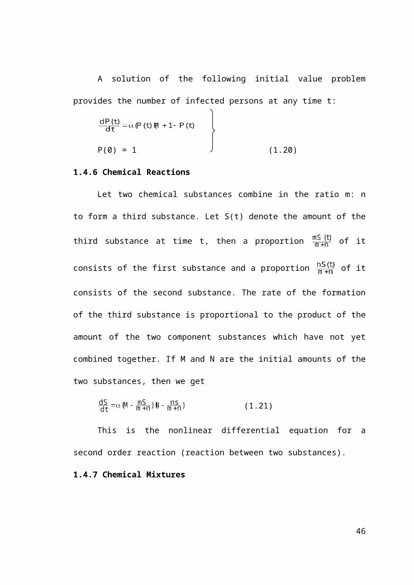
A solution of the following initial value problem provides the number of

infected persons at any time t:

31

P(0) = 1 (1.20)


Let two chemical substances combine in the ratio m: n to form a third

substance. Let S(t) denote the amount of the third substance at time t, then a

proportion of it consists of the first substance and a proportion of it

consists of the second substance. The rate of the formation of the third

substance is proportional to the product of the amount of the two component

substances which have not yet combined together. If M and N are the initial

amounts of the two substances, then we get

(1.21)

This is the nonlinear differential equation for a second order reaction

(reaction between two substances).


Let us suppose that a large mixing tank holds m gallons of water in which

salt has been dissolved. Assume that another brine solution is pumped into the

large tank at the rate of n gallons per minute, and then after proper mixing of

these ingredients it is pumped out at the same rate. Let us assume that the

concentration of the solution entering is p kilogram per gallon.

Let P(t) be the amount of salt (measured in kilograms) in the tank at any

time. Then the rate at which P(t) changes is a net rate:

=R1 - R2, say (1.22)

32

The rate R1 at which the salt enters the tank in kg/min is given by

R1 = (n gal/min).(p kg) = n.p

The rate R2 at which salt is leaving is given by

R2 = (n gal/min).(P/m kg/gal)

Then equation (1.22) becomes

The solution of (1.23) will provide the amount of salt at any time t.


Figure 1.3

Let the cylindrical container shown in Figure 1.3 have a constant cross-

section area A. The orifice at the base of the container has a constant cross-

sectional area B. If the container is filled with water to a height h, water will flow

out through the orifice.

Let h be the height of the water at time t, and let h+h be the height at

time t+t. Then volume of water lost when the level drops by an amount

h = volume of water that escapes through the orifice.

33

The volume of water lost in time t is given by -Ah, where the negative

sign indicates that the volume is a loss. The volume of water flowing through the

orifice in time t is the volume contained in a cylinder of cross section B and

length s. Thus we have

-Ah=Bs

Dividing by t and taking the limit as to, we get

(1.24)

where ds/st is the velocity of the water through the orifice. The velocity of

the water issuing from the orifice decreases as the level of the water decreases

and is given by famous Torricelli’s law of hydrodynamics to be

(1.25)

By (1.24) and (1.25) we get

(1.26)

Differential equation (1.2.6) is the model of the rate at which the water

level is dropping.

34


Figure 1.4

Let L = inductance, C = Capacitance, R = resistance be constant.

Consider the single-loop series circuit containing an inductor, resistor, and

capacitor shown in Figure 1.4. Let I(t) denote the amount of current after switch is

closed, let the charge on a capacitor at time is denoted by Q(t). Let E(t) denote

impressed voltage on a closed loop. According to Kirchhoffs' second law, the

impressed voltage E(t) on a closed loop must equal the sum of the voltage drops

in the loop. Current I(t) is related to Q(t) on the capacitor by

By adding the three voltage drops

Inductor Resistor Capacitor

and equating the sum to the impressed voltage, we obtain a second order

differential equation

35

1.4.10 Falling Body

According to Newton's first law of motion, a body will either remain at rest

or will continue to move with a constant velocity unless acted upon by an external

force. This implies that if the net force (resultant force) acting on a body is zero

then acceleration of the body is zero. According to Newton's second law of

motion, the net force on a body is proportional to its acceleration, provided the

net force acting on the body is not zero. That is if F0 is net force, m is the mass

of the body and A is the acceleration then F=mA.

Let a rock be tossed upward from the roof of a building. Let s(t) denote the

position of the rock relative to ground at time t. Then ds/dt and d 2s/dt2 are

respectively velocity and acceleration of the rock. By Newton's second law

The minus sign in (1.28) is used because the weight of the rock is a force

directed downwards which is opposite to the positive direction.

The position s(t) of the rock is the solution of the following initial-value

problem:

s(0)-s0, s'(0) = vo (1.29)

where so denotes the height of the roof of the given building and o denote

the initial velocity of the rock. We will discuss solutions of the problem of the type

(1.29)

in the subsequent chapters.

36


Persons having severe kidney disease frequently need toxic waste

products removed from their body by dialysis using an artificial kidney.

Essentially, an artificial kidney comprises two chambers separated by a

permeable membrane. The blood to be purified is passed through one chamber

while a cleaning fluid, called a dialysate, flows in the opposite direction through

the other. The pores in the membrane are small enough to prevent the passage

of blood cells but large enough to allow passage of the waste molecules. This is

shown schematically in figure 1.5 below

Figure 1.5

German physiologist Adolph Fick (1821-1901) showed that the net flow of

a substance separated by a membrane is from high concentration to low

concentration and that the amount of a substance that will pass through a

membrane in a unit time in proportional to the difference in the concentration

levels of the substance on each side of the membrane. This fact is often called

Fick's law.

In the artificial kidney, the concentration of waste in the blood is high and

that in dialysate is low, thus the waste molecules flow from the blood to the

37

dialysate. Let cb=cb(t) be the waste concentration in the blood and let cd=cd(t) be

the waste concentration in the dialysate. It is clear that cb(t)>cd(t).

Let us assume that the waste removal rate depends on the flow rate of

substance on each side of the membrane and that the following equation is valid

for the waste in the blood.

[Mass flow in] = [Mass lost through membrane]+[Mass flow out]

Lt Rb denote the blood flow rate then the mass flow rate of waste into the

machine is Rb.cb(t).

The amount of waste passing through the membrane in time t is k[cb(t)-

cd(t)]t by Ficks law and the mass flow of waste in the blood after t time is

Rb.cb(t+t). Thus we have

Rb.cb(t) = k[cb(t)-cd(t)]t+Rb.cb(t+t).

This equation can be arranged into the form

By taking the limit as to, we get

Equation (1.30) is a model of an artificial kidney whose solution will give us

concentration of waste in the blood at any time t.

38


Problem of survivability with AIDS (Acquired immunodeficiency syndrome)

after being infected with the human immunodeficiency virus (HIV) is a

challenging problem of the present time. Let t denote the elapsed time after

members of a group of HIV-infected people develop clinical AIDS. Let S(t) denote

the fraction of the group that remains alive at time t. One possible survival model

asserts that AIDS is not a fatal condition for a fraction of this group, denoted by

Si, to be called the immortal fraction here. 'For the remaining part of the group,

the probability of dying per unit time at time t will assumed to be constant k. Thus

the survival fraction S(t) for this model is a solution of the first order differential

equation.

where k must be positive.

The solution of (1.31) will be discussed in Chapter 4.

Example 1.18 Under the assumption of (1.8), find a differential equation

governing population N(t) of a country when individuals are allowed to migrate

from the country at a constant rate r.

Solution: The desired differential equation is

Example 1.19 At time t=o a technological innovation is introduced into a locality

of Delhi with fixed population of n people. Determine a mathematical model in the

39

form of a differential equation of the first order providing the number of people

x(t) who have adopted the innovation any time.

Solution. Let x(t) and y(t) denote respectively the number of people who have

adopted the innovation and those who have not adopted it. If one person who

has adopted the innovation is introduced into the population then x+y = n+1 and

x(0) = 1

We get this model following the argument of Section 1.5.

Example 1.20 The velocity of a particle in a magnetic field is found to be directly

proportional to the square root of its displacement. Determine a model in terms of

a differential equation of first-order of this situation.

Solution: Let x(t) be the displacement at time t.

Then speed = This means that

where

k is the constant of proportionality.

Example 1.21 If the time-rate of change of the demand D for a product is directly

proportional to elapsed time and inversely proportional to the square root of the

demand, then determine a differential equation describing this situation.

Solution: It is clear that the rate of change of D with respect to time t is

proportional to

. That is

40

,

where k is the constant of proportionality

Example 1.22. In the theory of learning, the rate at which a subject is memorized

is assumed to be proportional to the amount that is left to be memorized.

Suppose M denotes the total amount of a subject to be memorized and A(t) is the

amount memorized in time t. Write a differential equation for the amount A(t).

Solution: The rate of change , of the amount to be memorized is

proportional to M-A, that is

Exercises

1. Classify the given differential equation by order, and tell whether it is

linear or non linear.

(a) y’+2xy = x2 (b) y’ (y+x) = 5

(c) y sin y = y’’ (d) y cos y = y’’’

(e) cos y dy = sin x dx (f) y’’ = ey

2. State whether the given differential equation is linear or non linear.

Write the order of each equation.

(a) (1-x)y’’-6xy’+9y = sin x

(b)

(c) yy’ + 2y = 2 + x2

(d)

41

(e)

(f)

3. Verify that, in problems 3 to 8 the indicated function is a solution of the

given differential equation. In some cases assume an appropriate interval

3. 2y’+y = 0; y = e-x/2

4. y’=25+y2; y= 5 tan 5x

5. x2dy+2xy dx=0; y = -1/x2

6. y’’’-3y’’+3y’-y=0; y=x2ex

7. y’=y+1; y=ex-1

8. y’’+9y=8 sin x; y=sin x +c1 cos 3x+c2 sin 3x

In problems 9-14 determine a region of the xy plane for which the given

differential equation would have a unique solution through a point (xo,yo) in the

region

9.

10.

11.

12.

13.

14.

15. Derive a population growth model where death is taken into account.

42

16. A drug is infused into a patient's blood stream at a constant rate of r

g/s. Simultaneously the drug is removed at a rate proportional to the amount x(t)

of the drug present at any time t. Determine a differential equation governing the

amount x(t).

17. Find the relation between doubling and tripling times for a

population.

18. In an archaeological wooden specimen, only 25% of original radio

carbon 12 is present. Write a mathematical model, the solution of which will give

time of its manufacturing.

19. Write a mathematical model the solution of which will provide the rate

of interest compounded continuously if a bank's rate of interest is 10% per

annum?

20. The number of field mice in a certain pasture is given by the function

200-10t, where t is measured in years. Determine a differential equation

governing a population of owls that feed on the mice if the rate at which the owl

population grows is proportional to the difference between the number of owls at

time t and the number of field mice at time t.

21. Let a dog start running pursuing a rabbit at time to when the dog sights

the rabbit. Determine a differential equation (mathematical model) the solution of

which will give the path of pursuit assuming that the rabbit runs in a straight line

at a constant speed away from the dog and the dog runs at a constant speed so

that its line of sight is always directed at the rabbit.

43

22. To save money the manager of a manufacturing firm decides to

eliminate the advertising budget. In the absence of advertising, the sales

manager finds that sales, in rupees, decline at a rate that is directly proportional

to the volume of sales. Write a differential equation that describes the rate of

declining sales.

23. Suppose you deposited 10,000 Indian rupees in a bank account at

an interest rate of 5% compounded continuously. Write a mathematical model in

terms of differential equation, the solution of which will give the amount of money

in your account after a year and half.

24. Bacteria grown in a culture increase at a rate proportional to the

number present. If the number of bacteria doubles every 2 hours, then write a

mathematical equation describing this situation by which you can find the

population of bacteria (number of bacteria) after a given time say 10 hours, 10

days etc.

25. The schematic diagram in Figure 1.6 represents an electric circuit

in which a voltage of V volts in applied to a resistance of R Ohms and an

inductance of L henrys connected in series. When the switch is closed, a current

of I amperes will flow in the circuit. Because of the inductance in the circuit the

current will vary with time, and it can be shown that a mathematical model for this

circuit is the first order differential equation

44

Figure 1.6

Verify that the current in the circuit is given by

26. When an object at room temperature is placed in an oven whose

temperature is 400C0, the temperature of the object will increase with time,

approaching the temperature of the oven. It is known that the temperature Q of

the object is related to time through the differential equation

Verify that the temperature of the object is given by Q=400+cct, where c

and are constants.

27. Suppose that a large mixing tank initially holds 300 gallons of water

in which 50 pounds of salt has been dissolved. Pure water is pumped into the

tank at a rate of 3 gal/min, and then when solution is well stirred it is pumped out

at the same rate. Write a differential equation for the amount A(t) of salt in the

tank at any time t.

28. A spherical rain drop evaporates at a rate proportional to its surface

area. Write a differential equation which gives formula for its volume V as a

function of time.

29. A chemical A in a solution breaks down to form chemical B at a rate

proportional to the concentration of unconverted A. Half of A is converted in 20

minutes. Write down a differential equation describing this physical situation.

45

30. A fussy coffee brewer wants his water at 185oF but he often forgets

and lets it boil. Having broken his thermometer, he asks you to calculate how

long he should wait for it to cool from 212o to 185o . Can you solve his problem? If

you answer "Yes" do so. If no, then give explanation.

31. A car leaves at 11.30 am and arrives at Escort Heart Research Centre

Delhi at 3 pm. He started from rest and steadily increased his speed, as indicated

on his speedometer, to the extent that when he reached the destination he was

driving at the speed 60km per hour. Write a mathematical model in terms of

differential equation which may help to determine the location from where the car

started.

32. The growth rate of a population of bacteria is directly proportional to

the population. If the number of bacteria in a culture grow from 100 to 400 in 24

hours, write down the initial value problem which helps to determine the

population after 12 hours.

33. A man eats a diet of 2500 cal/day, 1200 of them go to basal

metabolism, that is get used up automatically. He spends approximately 16

cal/kg/day times his body weight (in kilograms) in weight-proportional exercise

Assume that storage of calories as fat is 100% efficient and that 1Kg fat contains

10,000 cal. Write down a mathematical model in terms of differential equation

giving variation of weight with time t.

34. Human skeletal fragments showing ancient Neanderthal

characteristics are found in a excavation and brought to laboratory for carbon

dating. Describe the model whose solution will provide the period during which

46

this person lived under the assumption that the proportion of C-14 to C-12 is only

6.24%.

35. Write down a mathematical model, solution of which will provide

time t during that the water flow out of an opening 0.5 cm2 at the bottom of a

conic funnel 10cm high, with the vector angle =60o.

36. Write an essay on the Van Meegeren Art Forgeries indicating role

of mathematical methods.

37. Charcoal from the occupation level of the famous Lascaux Cave in

France gave an average count in 1950 of .97 dis/min/g. Living wood gave 6.68

disintegrations. Write down a mathematical model, solution of that will give

probable date of the paintings found in the Lascaux Cave.

47

preface - faculty personal homepage- kfupmfaculty.kfupm.edu.sa/math/ahasan/coursecontents/chapter...

Documents