preface - cms.dm.uba.ar

Preface

My primary goal in writing Understanding Analysis was to create an elemen-tary one-semester book that exposes students to the rich rewards inherent intaking a mathematically rigorous approach to the study of functions of a realvariable. The aim of a course in real analysis should be to challenge and im-prove mathematical intuition rather than to verify it. There is a tendency,however, to center an introductory course too closely around the familiar the-orems of the standard calculus sequence. Producing a rigorous argument thatpolynomials are continuous is good evidence for a well-chosen definition of con-tinuity, but it is not the reason the subject was created and certainly not thereason it should be required study. By shifting the focus to topics where anuntrained intuition is severely disadvantaged (e.g., rearrangements of infiniteseries, nowhere-differentiable continuous functions, Fourier series), my intentis to restore an intellectual liveliness to this course by offering the beginningstudent access to some truly significant achievements of the subject.

The Main Objectives

In recent years, the standard undergraduate curriculum in mathematics hasbeen subjected to steady pressure from several different sources. As computersand technology become more ubiquitous, so do the areas where mathematicalthinking can be a valuable asset. Rather than preparing themselves for graduatestudy in pure mathematics, the present majority of mathematics majors lookforward to careers in banking, medicine, law, and numerous other fields whereanalytical skills are desirable. Another strong influence on college mathemat-ics is the ongoing calculus reform effort, now well over ten years old. At thecore of this movement is the justifiable goal of presenting calculus in a moreintuitive way, emphasizing geometric arguments over symbolic ones. Despitethese various trends—or perhaps because of them—nearly every undergraduatemathematics program continues to require at least one semester of real analysis.The result is that instructors today are faced with the task of teaching a diffi-cult, abstract course to a more diverse audience less familiar with the nature ofaxiomatic arguments.

The crux of the matter is that any prevailing sentiment in favor of marketingmathematics to larger groups must at some point be reconciled with the fact

v

vi Preface

that theoretical analysis is extremely challenging and even intimidating for some.One unfortunate resolution of this dilemma has been to make the course easierby making it less interesting. The omitted material is inevitably what givesanalysis its true flavor. A better solution is to find a way to make the moreadvanced topics accessible and worth the effort.

I see three essential goals that a semester of real analysis should try to meet:

1. Students, especially those emerging from a reform approach to calculus,need to be convinced of the need for a more rigorous study of functions.The necessity of precise definitions and an axiomatic approach must becarefully motivated.

2. Having seen mainly graphical, numerical, or intuitive arguments, studentsneed to learn what constitutes a rigorous mathematical proof and how towrite one.

3. There needs to be significant reward for the difficult work of firming up thelogical structure of limits. Specifically, real analysis should not be just anelaborate reworking of standard introductory calculus. Students shouldbe exposed to the tantalizing complexities of the real line, to the subtletiesof different flavors of convergence, and to the intellectual delights hiddenin the paradoxes of the infinite.

The philosophy of Understanding Analysis is to focus attention on questionsthat give analysis its inherent fascination. Does the Cantor set contain anyirrational numbers? Can the set of points where a function is discontinuousbe arbitrary? Are derivatives continuous? Are derivatives integrable? Is aninfinitely differentiable function necessarily the limit of its Taylor series? Ingiving these topics center stage, the hard work of a rigorous study is justifiedby the fact that they are inaccessible without it.

The Structure of the Book

This book is an introductory text. Although some fairly sophisticated topicsare brought in early to advertise and motivate the upcoming material, the mainbody of each chapter consists of a lean and focused treatment of the core top-ics that make up the center of most courses in analysis. Fundamental resultsabout completeness, compactness, sequential and functional limits, continuity,uniform convergence, differentiation, and integration are all incorporated. Whatis specific here is where the emphasis is placed. In the chapter on integration,for instance, the exposition revolves around deciphering the relationship be-tween continuity and the Riemann integral. Enough properties of the integralare obtained to justify a proof of the Fundamental Theorem of Calculus, butthe theme of the chapter is the pursuit of a characterization of integrable func-tions in terms of continuity. Whether or not Lebesgue’s measure-zero criterionis treated, framing the material in this way is still valuable because it is thequestions that are important. Mathematics is not a static discipline. Students

Preface vii

should be aware of the historical reasons for the creation of the mathematicsthey are learning and by extension realize that there is no last word on thesubject. In the case of integration, this point is made explicitly by includingsome relatively recent developments on the generalized Riemann integral in theadditional topics of the last chapter.

The structure of the chapters has the following distinctive features.

Discussion Sections: Each chapter begins with the discussion of some mo-tivating examples and open questions. The tone in these discussions is inten-tionally informal, and full use is made of familiar functions and results fromcalculus. The idea is to freely explore the terrain, providing context for theupcoming definitions and theorems. A recurring theme is the resolution of theparadoxes that arise when operations that work well in finite settings are naivelyextended to infinite settings (e.g., differentiating an infinite series term-by-term,reversing the order of a double summation). After these exploratory introduc-tions, the tone of the writing changes, and the treatment becomes rigorouslytight but still not overly formal. With the questions in place, the need for theensuing development of the material is well-motivated and the payoff is in sight.

Project Sections: The penultimate section of each chapter (the final section isa short epilogue) is written with the exercises incorporated into the exposition.Proofs are outlined but not completed, and additional exercises are includedto elucidate the material being discussed. The point of this is to provide someflexibility. The sections are written as self-guided tutorials, but they can alsobe the subject of lectures. I have used them in place of a final examination,and they work especially well as collaborative assignments that can culminatein a class presentation. The body of each chapter contains the necessary tools,so there is some satisfaction in letting the students use their newly acquiredskills to ferret out for themselves answers to questions that have been drivingthe exposition.

Building a Course

Teaching a satisfying class inevitably involves a race against time. Althoughthis book is designed for a 12–14 week semester, there are still a few choices tomake as to what to cover.

• The introductions can be discussed, assigned as reading, omitted, or sub-stituted with something preferable. There are no theorems proved herethat show up later in the text. I do develop some important examples inthese introductions (the Cantor set, Dirichlet’s nowhere-continuous func-tion) that probably need to find their way into discussions at some point.

• Chapter 3, Basic Topology of R, is much longer than it needs to be. Allthat is required by the ensuing chapters are fundamental results aboutopen and closed sets and a thorough understanding of sequential com-pactness. The characterization of compactness using open covers as well

viii Preface

as the section on perfect and connected sets are included for their own in-trinsic interest. They are not, however, crucial to any future proofs. Theone exception to this is a presentation of the Intermediate Value Theorem(IVT) as a special case of the preservation of connected sets by continu-ous functions. To keep connectedness truly optional, I have included twodirect proofs of IVT, one using least upper bounds and the other usingnested intervals. A similar comment can be made about perfect sets. Al-though proofs of the Baire Category Theorem are nicely motivated by theargument that perfect sets are uncountable, it is certainly possible to doone without the other.

• All the project sections (1.5, 2.8, 3.5, 4.6, 5.4, 6.6, 7.6, 8.1–8.4) are optionalin the sense that no results in later chapters depend on material in thesesections. The four topics covered in Chapter 8 are also written in thisproject-style format, where the exercises make up a significant part of thedevelopment. The only one of these sections that might require a lectureis the unit on Fourier series, which is a bit longer than the others.

The Audience

The only prerequisite for this course is a robust understanding of the resultsfrom single-variable calculus. The theorems of linear algebra are not needed,but the exposure to abstract arguments and proof writing that usually comeswith this course would be a valuable asset. Complex numbers are never used inthis book.

The proofs in Understanding Analysis are written with the introductorystudent firmly in mind. Brevity and other stylistic concerns are postponed infavor of including a significant level of detail. Most proofs come with a fairamount of discussion about the context of the argument. What should theproof entail? Which definitions are relevant? What is the overall strategy?Is one particular proof similar to something already done? Whenever there isa choice, efficiency is traded for an opportunity to reinforce some previouslylearned technique. Especially familiar or predictable arguments are usuallysketched as exercises so that students can participate directly in the developmentof the core material.

The search for recurring ideas exists at the proof-writing level and also onthe larger expository level. I have tried to give the course a narrative tone bypicking up on the unifying themes of approximation and the transition from thefinite to the infinite. To paraphrase a passage from the end of the book, realnumbers are approximated by rational ones; values of continuous functions areapproximated by values nearby; curves are approximated by straight lines; areasare approximated by sums of rectangles; continuous functions are approximatedby polynomials. In each case, the approximating objects are tangible and well-understood, and the issue is when and how well these qualities survive thelimiting process. By focusing on this recurring pattern, each successive topic

Preface ix

builds on the intuition of the previous one. The questions seem more natural,and a method to the madness emerges from what might otherwise appear as along list of theorems and proofs.

This book always emphasizes core ideas over generality, and it makes noeffort to be a complete, deductive catalog of results. It is designed to capture theintellectual imagination. Those who become interested are then exceptionallywell prepared for a second course starting from complex-valued functions onmore general spaces, while those content with a single semester come away witha strong sense of the essence and purpose of real analysis. Turning once moreto the concluding passages of Chapter 8, “By viewing the different infinities ofmathematics through pathways crafted out of finite objects, Weierstrass andthe other founders of analysis created a paradigm for how to extend the scopeof mathematical exploration deep into territory previously unattainable.”

This exploration has constituted the major thrill of my intellectual life. Iam extremely pleased to offer this guide to what I feel are some of the mostimpressive highlights of the journey. Have a wonderful trip!

Acknowledgments

The genesis of this book came from an extended series of conversations withBenjamin Lotto of Vassar College. The structure of the early chapters andthe book’s overall thesis are in large part the result of several years of sharingclassroom notes, ideas, and experiences with Ben. I am pleased with how themanuscript has turned out, and I have no doubt that it is an immeasurablybetter book because of Ben’s early contributions.

A large part of the writing was done while I was enjoying a visiting position atthe University of Virginia. Special thanks go to Nat Martin and Larry Thomasfor being so generous with their time and wisdom, and especially to LorenPitt, the scope of whose advice extends well beyond the covers of this book. Iwould also like to thank Julie Riddleberger for her help with many of the figures.Marian Robbins of Bellarmine College, Steve Kennedy of Carleton College, PaulHumke of Saint Olaf College, and Tom Kriete of the University of Virginia eachtaught from a preliminary draft of this text. I appreciate the many suggestedimprovements that this group provided, and I want to especially acknowledgePaul Humke for his contributions to the chapter on integration.

My department and the administration of Middlebury College have alsobeen very supportive of this endeavor. David Guertin came to my technologi-cal rescue on numerous occasions, Priscilla Bremser read early chapter drafts,and Rick Chartrand’s insightful opinions greatly improved some of the latersections. The list of students who have suffered through the long evolution ofthis book is now too long to present, but I would like to mention Brooke Sar-gent, whose meticulous class notes were the basis of the first draft, and JesseJohnson, who has worked tirelessly to improve the presentation of the manyexercises in the book. The production team at Springer has been absolutelyfirst-rate. My sincere thanks goes to all of them with a special nod to Sheldon

x Preface

Axler for encouragement and advice surely exceeding anything in his usual jobdescription.

In a recent rereading of the completed text, I was struck by how frequentlyI resort to historical context to motivate an idea. This was not a conscious goalI set for myself. Instead, I feel it is a reflection of a very encouraging trend inmathematical pedagogy to humanize our subject with its history. From my ownexperience, a good deal of the credit for this movement in analysis should goto two books: A Radical Approach to Real Analysis, by David Bressoud, andAnalysis by Its History, by E. Hairer and G. Wanner. Bressoud’s book wasparticularly influential to the presentation of Fourier series in the last chapter.Either of these would make an excellent supplementary resource for this course.While I do my best to cite their historical origins when it seems illuminating orespecially important, the present form of many of the theorems presented herebelongs to the common folklore of the subject, and I have not attempted carefulattribution. One exception is the material on the previously mentioned gen-eralized Riemann integral, due independently to Jaroslav Kurzweil and RalphHenstock. Section 8.1 closely follows the treatment laid out in Robert Bartle’sarticle “Return to the Riemann Integral.” In this paper, the author makes anitalicized plea for teachers of mathematics to supplant Lebesgue’s ubiquitousintegral with the generalized Riemann integral. I hope that Professor Bartlewill see its inclusion here as an inspired response to that request.

On a personal note, I welcome comments of any nature, and I will happilyshare any enlightening remarks—and any corrections—via a link on my web-page. The publication of this book comes nearly four years after the idea wasfirst hatched. The long road to this point has required the steady support ofmany people but most notably that of my incredible wife, Katy. Amid theflurry of difficult decisions and hard work that go into a project of this size, theopportunity to dedicate this book to her comes as a pure and easy pleasure.

Middlebury, Vermont Stephen AbbottAugust 2000

Contents

Preface v

1 The Real Numbers 11.1 Discussion: The Irrationality of

√2 . . . . . . . . . . . . . . . . . 1

1.2 Some Preliminaries . . . . . . . . . . . . . . . . . . . . . . . . . . 41.3 The Axiom of Completeness . . . . . . . . . . . . . . . . . . . . . 131.4 Consequences of Completeness . . . . . . . . . . . . . . . . . . . 181.5 Cantor’s Theorem . . . . . . . . . . . . . . . . . . . . . . . . . . 291.6 Epilogue . . . . . . . . . . . . . . . . . . . . . . . . . . . . . . . . 33

2 Sequences and Series 352.1 Discussion: Rearrangements of Infinite Series . . . . . . . . . . . 352.2 The Limit of a Sequence . . . . . . . . . . . . . . . . . . . . . . . 382.3 The Algebraic and Order Limit Theorems . . . . . . . . . . . . . 442.4 The Monotone Convergence Theorem and a First Look at

Infinite Series . . . . . . . . . . . . . . . . . . . . . . . . . . . . . 502.5 Subsequences and the Bolzano–Weierstrass Theorem . . . . . . . 552.6 The Cauchy Criterion . . . . . . . . . . . . . . . . . . . . . . . . 582.7 Properties of Infinite Series . . . . . . . . . . . . . . . . . . . . . 622.8 Double Summations and Products of Infinite Series . . . . . . . . 692.9 Epilogue . . . . . . . . . . . . . . . . . . . . . . . . . . . . . . . . 73

3 Basic Topology of R 753.1 Discussion: The Cantor Set . . . . . . . . . . . . . . . . . . . . . 753.2 Open and Closed Sets . . . . . . . . . . . . . . . . . . . . . . . . 783.3 Compact Sets . . . . . . . . . . . . . . . . . . . . . . . . . . . . . 843.4 Perfect Sets and Connected Sets . . . . . . . . . . . . . . . . . . 893.5 Baire’s Theorem . . . . . . . . . . . . . . . . . . . . . . . . . . . 943.6 Epilogue . . . . . . . . . . . . . . . . . . . . . . . . . . . . . . . . 96

4 Functional Limits and Continuity 994.1 Discussion: Examples of Dirichlet and Thomae . . . . . . . . . . 994.2 Functional Limits . . . . . . . . . . . . . . . . . . . . . . . . . . . 1034.3 Combinations of Continuous Functions . . . . . . . . . . . . . . . 109

xi

xii Contents

4.4 Continuous Functions on Compact Sets . . . . . . . . . . . . . . 1144.5 The Intermediate Value Theorem . . . . . . . . . . . . . . . . . . 1204.6 Sets of Discontinuity . . . . . . . . . . . . . . . . . . . . . . . . . 1254.7 Epilogue . . . . . . . . . . . . . . . . . . . . . . . . . . . . . . . . 127

5 The Derivative 1295.1 Discussion: Are Derivatives Continuous? . . . . . . . . . . . . . . 1295.2 Derivatives and the Intermediate Value Property . . . . . . . . . 1315.3 The Mean Value Theorem . . . . . . . . . . . . . . . . . . . . . . 1375.4 A Continuous Nowhere-Differentiable Function . . . . . . . . . . 1445.5 Epilogue . . . . . . . . . . . . . . . . . . . . . . . . . . . . . . . . 148

6 Sequences and Series of Functions 1516.1 Discussion: Branching Processes . . . . . . . . . . . . . . . . . . 1516.2 Uniform Convergence of a Sequence of Functions . . . . . . . . . 1546.3 Uniform Convergence and Differentiation . . . . . . . . . . . . . 1646.4 Series of Functions . . . . . . . . . . . . . . . . . . . . . . . . . . 1676.5 Power Series . . . . . . . . . . . . . . . . . . . . . . . . . . . . . . 1696.6 Taylor Series . . . . . . . . . . . . . . . . . . . . . . . . . . . . . 1766.7 Epilogue . . . . . . . . . . . . . . . . . . . . . . . . . . . . . . . . 181

7 The Riemann Integral 1837.1 Discussion: How Should Integration be Defined? . . . . . . . . . 1837.2 The Definition of the Riemann Integral . . . . . . . . . . . . . . . 1867.3 Integrating Functions with Discontinuities . . . . . . . . . . . . . 1917.4 Properties of the Integral . . . . . . . . . . . . . . . . . . . . . . 1957.5 The Fundamental Theorem of Calculus . . . . . . . . . . . . . . . 1997.6 Lebesgue’s Criterion for Riemann Integrability . . . . . . . . . . 2037.7 Epilogue . . . . . . . . . . . . . . . . . . . . . . . . . . . . . . . . 210

8 Additional Topics 2138.1 The Generalized Riemann Integral . . . . . . . . . . . . . . . . . 2138.2 Metric Spaces and the Baire Category Theorem . . . . . . . . . . 2228.3 Fourier Series . . . . . . . . . . . . . . . . . . . . . . . . . . . . . 2288.4 A Construction of R From Q . . . . . . . . . . . . . . . . . . . . 243

Bibliography 251

Index 253

Chapter 1

The Real Numbers

1.1 Discussion: The Irrationality of√

2Toward the end of his distinguished career, the renowned British mathematicianG.H. Hardy eloquently laid out a justification for a life of studying mathematicsin A Mathematician’s Apology, an essay first published in 1940. At the centerof Hardy’s defense is the thesis that mathematics is an aesthetic discipline. ForHardy, the applied mathematics of engineers and economists held little charm.“Real mathematics,” as he referred to it, “must be justified as art if it can bejustified at all.”

To help make his point, Hardy includes two theorems from classical Greekmathematics, which, in his opinion, possess an elusive kind of beauty that,although difficult to define, is easy to recognize. The first of these results isEuclid’s proof that there are an infinite number of prime numbers. The secondresult is the discovery, attributed to the school of Pythagoras from around 500B.C., that

√2 is irrational. It is this second theorem that demands our attention.

(A course in number theory would focus on the first.) The argument uses onlyarithmetic, but its depth and importance cannot be overstated. As Hardy says,“[It] is a ‘simple’ theorem, simple both in idea and execution, but there is nodoubt at all about [it being] of the highest class. [It] is as fresh and significantas when it was discovered—two thousand years have not written a wrinkle on[it].”

Theorem 1.1.1. There is no rational number whose square is 2.

Proof. A rational number is any number that can be expressed in the form p/q,where p and q are integers. Thus, what the theorem asserts is that no matterhow p and q are chosen, it is never the case that (p/q)2 = 2. The line of attackis indirect, using a type of argument referred to as a proof by contradiction.The idea is to assume that there is a rational number whose square is 2 andthen proceed along logical lines until we reach a conclusion that is unacceptable.At this point, we will be forced to retrace our steps and reject the erroneous

1

2 Chapter 1. The Real Numbers

assumption that some rational number squared is equal to 2. In short, we willprove that the theorem is true by demonstrating that it cannot be false.

And so assume, for contradiction, that there exist integers p and q satisfying

(1)(p

q

)2

= 2.

We may also assume that p and q have no common factor, because, if they hadone, we could simply cancel it out and rewrite the fraction in lowest terms. Now,equation (1) implies

(2) p2 = 2q2.

From this, we can see that the integer p2 is an even number (it is divisible by2), and hence p must be even as well because the square of an odd number isodd. This allows us to write p = 2r, where r is also an integer. If we substitute2r for p in equation (2), then a little algebra yields the relationship

2r2 = q2.

But now the absurdity is at hand. This last equation implies that q2 is even,and hence q must also be even. Thus, we have shown that p and q are botheven (i.e., divisible by 2) when they were originally assumed to have no commonfactor. From this logical impasse, we can only conclude that equation (1) cannothold for any integers p and q, and thus the theorem is proved.

A component of Hardy’s definition of beauty in a mathematical theoremis that the result have lasting and serious implications for a network of othermathematical ideas. In this case, the ideas under assault were the Greeks’ un-derstanding of the relationship between geometric length and arithmetic number.Prior to the preceding discovery, it was an assumed and commonly used factthat, given two line segments AB and CD, it would always be possible to finda third line segment whose length divides evenly into the first two. In modernterminology, this is equivalent to asserting that the length of CD is a rationalmultiple of the length of AB. Looking at the diagonal of a unit square (Fig.1.1), it now followed (using the Pythagorean Theorem) that this was not alwaysthe case. Because the Pythagoreans implicitly interpreted number to mean ra-tional number, they were forced to accept that number was a strictly weakernotion than length.

Rather than abandoning arithmetic in favor of geometry (as the Greeks seemto have done), our resolution to this limitation is to strengthen the concept ofnumber by moving from the rational numbers to a larger number system. Froma modern point of view, this should seem like a familiar and somewhat naturalphenomenon. We begin with the natural numbers

N = {1, 2, 3, 4, 5, . . . }.The influential German mathematician Leopold Kronecker (1823–1891) onceasserted that “The natural numbers are the work of God. All of the rest is

1.1. Discussion: The Irrationality of√2 3

��

CA B

D

1

1

√2

• •

•

Figure 1.1:√2 exists as a geometric length.

the work of mankind.” Debating the validity of this claim is an interestingconversation for another time. For the moment, it at least provides us witha place to start. If we restrict our attention to the natural numbers N, thenwe can perform addition perfectly well, but we must extend our system to theintegers

Z = {. . . ,−3,−2,−1, 0, 1, 2, 3, . . . }if we want to have an additive identity (zero) and the additive inverses necessaryto define subtraction. The next issue is multiplication and division. The number1 acts as the multiplicative identity, but in order to define division we need tohave multiplicative inverses. Thus, we extend our system again to the rationalnumbers

Q ={all fractions

p

qwhere p and q are integers with q �= 0

}.

Taken together, the properties of Q discussed in the previous paragraphessentially make up the definition of what is called a field. More formally stated,a field is any set where addition and multiplication are well-defined operationsthat are commutative, associative, and obey the familiar distributive propertya(b+ c) = ab+ ac. There must be an additive identity, and every element musthave an additive inverse. Finally, there must be a multiplicative identity, andmultiplicative inverses must exist for all nonzero elements of the field. NeitherZ nor N is a field. The finite set {0, 1, 2, 3, 4} is a field when addition andmultiplication are computed modulo 5. This is not immediately obvious butmakes an interesting exercise (Exercise 1.3.1).

The set Q also has a natural order defined on it. Given any two rationalnumbers r and s, exactly one of the following is true:

r < s, r = s, or r > s.

This ordering is transitive in the sense that if r < s and s < t, then r < t, sowe are conveniently led to a mental picture of the rational numbers as beinglaid out from left to right along a number line. Unlike Z, there are no intervalsof empty space. Given any two rational numbers r < s, the rational number


11.414

√2

1.5 2↑↓

Figure 1.2: Approximating√2 with rational numbers.

(r+s)/2 sits halfway in between, implying that the rational numbers are denselynestled together.

With the field properties of Q allowing us to safely carry out the algebraicoperations of addition, subtraction, multiplication, and division, let’s remindourselves just what it is that Q is lacking. By Theorem 1.1.1, it is apparentthat we cannot always take square roots. The problem, however, is actuallymore fundamental than this. Using only rational numbers, it is possible toapproximate

√2 quite well (Fig. 1.2). For instance, 1.4142 = 1.999396. By

adding more decimal places to our approximation, we can get even closer toa value for

√2, but, even so, we are now well aware that there is a “hole” in

the rational number line where√2 ought to be. Of course, there are quite a

few other holes—at√3 and

√5, for example. Returning to the dilemma of the

ancient Greek mathematicians, if we want every length along the number line tocorrespond to an actual number, then another extension to our number systemis in order. Thus, to the chain N ⊆ Z ⊆ Q we append the real numbers R.

The question of how to actually construct R from Q is rather complicatedbusiness. It is discussed in Section 1.3, and then again in more detail in Section8.4. For the moment, it is not too inaccurate to say that R is obtained byfilling in the gaps in Q. Wherever there is a hole, a new irrational number isdefined and placed into the ordering that already exists on Q. The real numbersare then the union of these irrational numbers together with the more familiarrational ones. What properties does the set of irrational numbers have? Howdo the sets of rational and irrational numbers fit together? Is there a kindof symmetry between the rationals and the irrationals, or is there some sensein which we can argue that one type of real number is more common than theother? The one method we have seen so far for generating examples of irrationalnumbers is through square roots. Not too surprisingly, other roots such as 3

√2

or 5√3 are most often irrational. Can all irrational numbers be expressed as

algebraic combinations of nth roots and rational numbers, or are there stillother irrational numbers beyond those of this form?

1.2 Some Preliminaries

The vocabulary necessary for the ensuing development comes from set theoryand the theory of functions. This should be familiar territory, but a brief review

1.2. Some Preliminaries 5

of the terminology is probably a good idea, if only to establish some agreed-uponnotation.

Sets

Intuitively speaking, a set is any collection of objects. These objects are referredto as the elements of the set. For our purposes, the sets in question will mostoften be sets of real numbers, although we will also encounter sets of functionsand, on a few rare occasions, sets whose elements are other sets.

Given a set A, we write x ∈ A if x (whatever it may be) is an element of A.If x is not an element of A, then we write x /∈ A. Given two sets A and B, theunion is written A ∪B and is defined by asserting that

x ∈ A ∪B provided that x ∈ A or x ∈ B (or potentially both).

The intersection A ∩B is the set defined by the rule

x ∈ A ∩B provided x ∈ A and x ∈ B.

Example 1.2.1. (i) There are many acceptable ways to assert the contents ofa set. In the previous section, the set of natural numbers was defined by listingthe elements: N = {1, 2, 3, . . . }.

(ii) Sets can also be described in words. For instance, we can define the setE to be the collection of even natural numbers.

(iii) Sometimes it is more efficient to provide a kind of rule or algorithm fordetermining the elements of a set. As an example, let

S = {r ∈ Q : r2 < 2}.

Read aloud, the definition of S says, “Let S be the set of all rational numberswhose squares are less than 2.” It follows that 1 ∈ S, 4/3 ∈ S, but 3/2 /∈ Sbecause 9/4 ≥ 2.

Using the previously defined sets to illustrate the operations of intersectionand union, we observe that

N ∪ E = N, N ∩ E = E, N ∩ S = {1}, and E ∩ S = ∅.

The set ∅ is called the empty set and is understood to be the set that contains noelements. An equivalent statement would be to say that E and S are disjoint.

A word about the equality of two sets is in order (since we have just usedthe notion). The inclusion relationship A ⊆ B or B ⊇ A is used to indicate thatevery element of A is also an element of B. In this case, we say A is a subset ofB, or B contains A. To assert that A = B means that A ⊆ B and B ⊆ A. Putanother way, A and B have exactly the same elements.

Quite frequently in the upcoming chapters, we will want to apply the unionand intersection operations to infinite collections of sets.


Example 1.2.2. Let

A1 = N = {1, 2, 3, . . . },A2 = {2, 3, 4, . . . },A3 = {3, 4, 5, . . . },

and, in general, for each n ∈ N, define the set

An = {n, n+ 1, n+ 2, . . . }.The result is a nested chain of sets

A1 ⊇ A2 ⊇ A3 ⊇ A4 ⊇ · · · ,where each successive set is a subset of all the previous ones. Notationally,

∞⋃n=1

An,⋃n∈N

An, or A1 ∪A2 ∪A3 ∪ · · ·

are all equivalent ways to indicate the set whose elements consist of any elementthat appears in at least one particular An. Because of the nested property ofthis particular collection of sets, it is not too hard to see that

∞⋃n=1

An = A1.

The notion of intersection has the same kind of natural extension to infinitecollections of sets. For this example, we have

∞⋂n=1

An = ∅.

Let’s be sure we understand why this is the case. Suppose we had some naturalnumber m that we thought might actually satisfy m ∈ ⋂∞

n=1 An. What thiswould mean is that m ∈ An for every An in our collection of sets. Because m isnot an element of Am+1, no such m exists and the intersection is empty.

As mentioned, most of the sets we encounter will be sets of real numbers.Given A ⊆ R, the complement of A, written Ac, refers to the set of all elementsof R not in A. Thus, for A ⊆ R,

Ac = {x ∈ R : x /∈ A}.A few times in our work to come, we will refer to De Morgan’s Laws, whichstate that

(A ∩B)c = Ac ∪Bc and (A ∪B)c = Ac ∩Bc.

Proofs of these statements are discussed in Exercise 1.2.3.


Admittedly, there is something imprecise about the definition of set pre-sented at the beginning of this discussion. The defining sentence begins withthe phrase “Intuitively speaking,” which might seem an odd way to embark on acourse of study that purportedly intends to supply a rigorous foundation for thetheory of functions of a real variable. In some sense, however, this is unavoid-able. Each repair of one level of the foundation reveals something below it inneed of attention. The theory of sets has been subjected to intense scrutiny overthe past century precisely because so much of modern mathematics rests on thisfoundation. But such a study is really only advisable once it is understood whyour naive impression about the behavior of sets is insufficient. For the directionin which we are heading, this will not happen, although an indication of somepotential pitfalls is given in Section 1.6.

Functions

Definition 1.2.3. Given two sets A and B, a function from A to B is a rule ormapping that takes each element x ∈ A and associates with it a single elementof B. In this case, we write f : A → B. Given an element x ∈ A, the expressionf(x) is used to represent the element of B associated with x by f . The set A iscalled the domain of f . The range of f is not necessarily equal to B but refersto the subset of B given by {y ∈ B : y = f(x) for some x ∈ A}.

This definition of function is more or less the one proposed by Peter LejeuneDirichlet (1805–1859) in the 1830s. Dirichlet was a German mathematician whowas one of the leaders in the development of the rigorous approach to functionsthat we are about to undertake. His main motivation was to unravel the issuessurrounding the convergence of Fourier series. Dirichlet’s contributions figureprominently in Section 8.3, where an introduction to Fourier series is presented,but we will also encounter his name in several earlier chapters along the way.What is important at the moment is that we see how Dirichlet’s definitionof function liberates the term from its interpretation as a type of “formula.”In the years leading up to Dirichlet’s time, the term “function” was generallyunderstood to refer to algebraic entities such as f(x) = x2+1 or g(x) =

√x4 + 4.

Definition 1.2.3 allows for a much broader range of possibilities.

Example 1.2.4. In 1829, Dirichlet proposed the unruly function

g(x) ={1 if x ∈ Q0 if x /∈ Q.

The domain of g is all of R, and the range is the set {0, 1}. There is no singleformula for g in the usual sense, and it is quite difficult to graph this function(see Section 4.1 for a rough attempt), but it certainly qualifies as a functionaccording to the criterion in Definition 1.2.3. As we study the theoretical natureof continuous, differentiable, or integrable functions, examples such as this onewill provide us with an invaluable testing ground for the many conjectures weencounter.


Example 1.2.5 (Triangle Inequality). The absolute value function is so im-portant that it merits the special notation |x| in place of the usual f(x) or g(x).It is defined for every real number via the piecewise definition

|x| ={

x if x ≥ 0−x if x < 0.

With respect to multiplication and division, the absolute value function satisfies

(i) |ab| = |a||b| and(ii) |a+ b| ≤ |a|+ |b|for all choices of a and b. Verifying these properties (Exercise 1.2.4) is just amatter of examining the different cases that arise when a, b, and a+b are positiveand negative. Property (ii) is called the triangle inequality. This innocuouslooking inequality turns out to be fantastically important and will be frequentlyemployed in the following way. Given three real numbers a, b, and c, we certainlyhave

|a− b| = |(a− c) + (c− b)|.By the triangle inequality,

|(a− c) + (c− b)| ≤ |a− c|+ |c− b|,

so we get

(1) |a− b| ≤ |a− c|+ |c− b|.

Now, the expression |a − b| is equal to |b − a| and is best understood as thedistance between the points a and b on the number line. With this interpretation,equation (1) makes the plausible statement that “the distance from a to b isless than or equal to the distance from a to c plus the distance from c to b.”Pretending for a moment that these are points in the plane (instead of on thereal line), it should be evident why this is referred to as the “triangle inequality.”

Logic and Proofs

Writing rigorous mathematical proofs is a skill best learned by doing, and thereis plenty of on-the-job training just ahead. As Hardy indicates, there is anartistic quality to mathematics of this type, which may or may not come easily,but that is not to say that anything especially mysterious is happening. Aproof is an essay of sorts. It is a set of carefully crafted directions, which,when followed, should leave the reader absolutely convinced of the truth ofthe proposition in question. To achieve this, the steps in a proof must followlogically from previous steps or be justified by some other agreed-upon set offacts. In addition to being valid, these steps must also fit coherently together toform a cogent argument. Mathematics has a specialized vocabulary, to be sure,


but that does not exempt a good proof from being written in grammaticallycorrect English.

The one proof we have seen at this point (to Theorem 1.1.1) uses an indirectstrategy called proof by contradiction. This powerful technique will be employeda number of times in our upcoming work. Nevertheless, most proofs are direct.(It also bears mentioning that using an indirect proof when a direct proof isavailable is generally considered bad manners.) A direct proof begins fromsome valid statement, most often taken from the theorem’s hypothesis, andthen proceeds through rigorously logical deductions to a demonstration of thetheorem’s conclusion. As we saw in Theorem 1.1.1, an indirect proof alwaysbegins by negating what it is we would like to prove. This is not always as easyto do as it may sound. The argument then proceeds until (hopefully) a logicalcontradiction with some other accepted fact is uncovered. Many times, thisaccepted fact is part of the hypothesis of the theorem. When the contradiction iswith the theorem’s hypothesis, we technically have what is called a contrapositiveproof.

The next proposition illustrates a number of the issues just discussed andintroduces a few more.

Theorem 1.2.6. Two real numbers a and b are equal if and only if for everyreal number ε > 0 it follows that |a− b| < ε.

Proof. There are two key phrases in the statement of this proposition thatwarrant special attention. One is “for every,” which will be addressed in amoment. The other is “if and only if.” To say “if and only if” in mathematicsis an economical way of stating that the proposition is true in two directions.In the forward direction, we must prove the statement:

(⇒) If a = b, then for every real number ε > 0 it follows that |a− b| < ε.We must also prove the converse statement:

(⇐) If for every real number ε > 0 it follows that |a− b| < ε, then we musthave a = b.

For the proof of the first statement, there is really not much to say. If a = b,then |a− b| = 0, and so certainly |a− b| < ε no matter what ε > 0 is chosen.

For the second statement, we give a proof by contradiction. The conclusionof the proposition in this direction states that a = b, so we assume that a �= b.Heading off in search of a contradiction brings us to a consideration of the phrase“for every ε > 0.” Some equivalent ways to state the hypothesis would be tosay that “for all possible choices of ε > 0” or “no matter how ε > 0 is selected,it is always the case that |a− b| < ε.” But assuming a �= b (as we are doing atthe moment), the choice of

ε0 = |a− b| > 0

poses a serious problem. We are assuming that |a − b| < ε is true for everyε > 0, so this must certainly be true of the particular ε0 just defined. However,the statements

|a− b| < ε0 and |a− b| = ε0


cannot both be true. This contradiction means that our initial assumption thata �= b is unacceptable. Therefore, a = b, and the indirect proof is complete.

One of the most fundamental skills required for reading and writing analysisproofs is the ability to confidently manipulate the quantifying phrases “for all”and “there exists.” Significantly more attention will be given to this issue inmany upcoming discussions.

Induction

One final trick of the trade, which will arise with some frequency, is the use ofinduction arguments. Induction is used in conjunction with the natural numbersN (or sometimes with the set N ∪ {0}). The fundamental principle behindinduction is that if S is some subset of N with the property that

(i) S contains 1 and

(ii) whenever S contains a natural number n, it also contains n+ 1,

then it must be that S = N. As the next example illustrates, this principle canbe used to define sequences of objects as well as to prove facts about them.

Example 1.2.7. Let x1 = 1, and for each n ∈ N define

xn+1 = (1/2)xn + 1.

Using this rule, we can compute x2 = (1/2)(1) + 1 = 3/2, x3 = 7/4, and it isimmediately apparent how this leads to a definition of xn for all n ∈ N.

The sequence just defined appears at the outset to be increasing. For theterms computed, we have x1 ≤ x2 ≤ x3. Let’s use induction to prove that thistrend continues; that is, let’s show

(2) xn ≤ xn+1

for all values of n ∈ N.For n = 1, x1 = 1 and x2 = 3/2, so that x1 ≤ x2 is clear. Now, we want to

show that

if we have xn ≤ xn+1, then it follows that xn+1 ≤ xn+2.

Think of S as the set of natural numbers for which the claim in equation (2)is true. We have shown that 1 ∈ S. We are now interested in showing that ifn ∈ S, then n+1 ∈ S as well. Starting from the induction hypothesis xn ≤ xn+1,we can multiply across the inequality by 1/2 and add 1 to get

12xn + 1 ≤ 1

2xn+1 + 1,

which is precisely the desired conclusion xn+1 ≤ xn+2. By induction, the claimis proved for all n ∈ N.


Any discussion about why induction is a valid argumentative technique im-mediately opens up a box of questions about how we understand the naturalnumbers. Earlier, in Section 1.1, we avoided this issue by referencing Kro-necker’s famous comment that the natural numbers are somehow divinely given.Although we will not improve on this explanation here, it should be pointed outthat a more atheistic and mathematically satisfying approach to N is possiblefrom the point of view of axiomatic set theory. This brings us back to a recurringtheme of this chapter. Pedagogically speaking, the foundations of mathematicsare best learned and appreciated in a kind of reverse order. A rigorous study ofthe natural numbers and the theory of sets is certainly recommended, but onlyafter we have an understanding of the subtleties of the real number system. Itis this latter topic that is the business of real analysis.

Exercises

Exercise 1.2.1. (a) Prove that√3 is irrational. Does a similar argument work

to show√6 is irrational?

(b) Where does the proof of Theorem 1.1.1 break down if we try to use it toprove

√4 is irrational?

Exercise 1.2.2. Decide which of the following represent true statements aboutthe nature of sets. For any that are false, provide a specific example where thestatement in question does not hold.

(a) If A1 ⊇ A2 ⊇ A3 ⊇ A4 · · · are all sets containing an infinite number ofelements, then the intersection ∩∞

n=1An is infinite as well.(b) If A1 ⊇ A2 ⊇ A3 ⊇ A4 · · · are all finite, nonempty sets of real numbers,

then the intersection ∩∞n=1An is finite and nonempty.

(c) A ∩ (B ∪ C) = (A ∩B) ∪ C.(d) A ∩ (B ∩ C) = (A ∩B) ∩ C.(e) A ∩ (B ∪ C) = (A ∩B) ∪ (A ∩ C).

Exercise 1.2.3 (De Morgan’s Laws). Let A and B be subsets of R.(a) If x ∈ (A ∩ B)c, explain why x ∈ Ac ∪ Bc. This shows that (A ∩ B)c ⊆

Ac ∪Bc.(b) Prove the reverse inclusion (A ∩ B)c ⊇ Ac ∪ Bc, and conclude that

(A ∩B)c = Ac ∪Bc.(c) Show (A ∪B)c = Ac ∩Bc by demonstrating inclusion both ways.

Exercise 1.2.4. Verify the triangle inequality in the special cases where(a) a and b have the same sign;(b) a ≥ 0, b < 0, and a+ b ≥ 0.

Exercise 1.2.5. Use the triangle inequality to establish the inequalities(a) |a− b| ≤ |a|+ |b|;(b) ||a| − |b|| ≤ |a− b|.

Exercise 1.2.6. Given a function f and a subset A of its domain, let f(A)represent the range of f over the set A; that is, f(A) = {f(x) : x ∈ A}.


(a) Let f(x) = x2. If A = [0, 2] (the closed interval {x ∈ R : 0 ≤ x ≤ 2})and B = [1, 4], find f(A) and f(B). Does f(A∩B) = f(A)∩ f(B) in this case?Does f(A ∪B) = f(A) ∪ f(B)?

(b) Find two sets A and B for which f(A ∩B) �= f(A) ∩ f(B).(c) Show that, for an arbitrary function g : R → R, it is always true that

g(A ∩B) ⊆ g(A) ∩ g(B) for all sets A,B ⊆ R.(d) Form and prove a conjecture about the relationship between g(A ∪ B)

and g(A) ∪ g(B) for an arbitrary function g.

Exercise 1.2.7. Given a function f : D → R and a subset B ⊆ R, let f−1(B)be the set of all points from the domain D that get mapped into B; that is,f−1(B) = {x ∈ D : f(x) ∈ B}. This set is called the preimage of B.

(a) Let f(x) = x2. If A is the closed interval [0, 4] and B is the closed interval[−1, 1], find f−1(A) and f−1(B). Does f−1(A ∩B) = f−1(A) ∩ f−1(B) in thiscase? Does f−1(A ∪B) = f−1(A) ∪ f−1(B)?

(b) The good behavior of preimages demonstrated in (a) is completely gen-eral. Show that for an arbitrary function g : R → R, it is always true thatg−1(A ∩B) = g−1(A) ∩ g−1(B) and g−1(A ∪B) = g−1(A) ∪ g−1(B) for all setsA,B ⊆ R.

Exercise 1.2.8. Form the logical negation of each claim. One way to do this isto simply add “It is not the case that...” in front of each assertion, but for eachstatement, try to embed the word “not” as deeply into the resulting sentenceas possible (or avoid using it altogether).

(a) For all real numbers satisfying a < b, there exists an n ∈ N such thata+ 1/n < b.

(b) Between every two distinct real numbers, there is a rational number.(c) For all natural numbers n ∈ N,

√n is either a natural number or an

irrational number.(d) Given any real number x ∈ R, there exists n ∈ N satisfying n > x.

Exercise 1.2.9. Show that the sequence (x1, x2, x3, . . . ) defined in Example1.2.7 is bounded above by 2; that is, prove that xn ≤ 2 for every n ∈ N.

Exercise 1.2.10. Let y1 = 1, and for each n ∈ N define yn+1 = (3yn + 4)/4.(a) Use induction to prove that the sequence satisfies yn < 4 for all n ∈ N.(b) Use another induction argument to show the sequence (y1, y2, y3, . . . ) is

increasing.

Exercise 1.2.11. If a set A contains n elements, prove that the number ofdifferent subsets of A is equal to 2n. (Keep in mind that the empty set ∅ isconsidered to be a subset of every set.)

Exercise 1.2.12. For this exercise, assume Exercise 1.2.3 has been successfullycompleted.

(a) Show how induction can be used to conclude that

(A1 ∪A2 ∪ · · · ∪An)c = Ac

1 ∩Ac2 ∩ · · · ∩Ac

n

1.3. The Axiom of Completeness 13

for any finite n ∈ N.(b) Explain why induction cannot be used to conclude( ∞⋃

n=1

An

)c

=∞⋂n=1

Acn.

It might be useful to consider part (a) of Exercise 1.2.2.(c) Is the statement in part (b) valid? If so, write a proof that does not use

induction.

1.3 The Axiom of Completeness

What exactly is a real number? In Section 1.1, we got as far as saying thatthe set R of real numbers is an extension of the rational numbers Q in whichthere are no holes or gaps. We want every length along the number line—suchas

√2—to correspond to a real number and vice versa.We are going to improve on this definition, but as we do so, it is important

to keep in mind our earlier acknowledgment that whatever precise statementswe formulate will necessarily rest on other unproven assumptions or undefinedterms. At some point, we must draw a line and confess that this is what we havedecided to accept as a reasonable place to start. Naturally, there is some debateabout where this line should be drawn. One way to view the mathematics ofthe 19th and 20th centuries is as a stalwart attempt to move this line furtherand further back toward some unshakable foundation. The majority of thematerial covered in this book is attributable to the mathematicians working inthe early and middle parts of the 1800s. Augustin Louis Cauchy (1789–1857),Bernhard Bolzano (1781–1848), Niels Henrik Abel (1802–1829), Peter LejeuneDirichlet, Karl Weierstrass (1815–1897), and Bernhard Riemann (1826–1866) allfigure prominently in the discovery of the theorems that follow. But here is theinteresting point. Nearly all of this work was done using intuitive assumptionsabout the nature of R quite similar to our own informal understanding at thispoint. Eventually, enough scrutiny was directed at the detailed structure of Rso that, in the 1870s, a handful of ways to rigorously construct R from Q wereproposed.

Following this historical model, our own rigorous construction of R from Qis postponed until Section 8.4. By this point, the need for such a constructionwill be more justified and easier to appreciate. In the meantime, we have manyproofs to write, so it is important to lay down, as explicitly as possible, theassumptions that we intend to make about the real numbers.

An Initial Definition for R

First, R is a set containing Q. The operations of addition and multiplicationon Q extend to all of R in such a way that every element of R has an additiveinverse and every nonzero element of R has a multiplicative inverse. Echoing


the discussion in Section 1.1, we assume R is a field, meaning that addition andmultiplication of real numbers is commutative, associative, and the distributiveproperty holds. This allows us to perform all of the standard algebraic manipu-lations that are second nature to us. We also assume that the familiar propertiesof the ordering on Q extend to all of R. Thus, for example, such deductions as“If a < b and c > 0, then ac < bc” will be carried out freely without much com-ment. To summarize the situation in the official terminology of the subject, weassume that R is an ordered field, which contains Q as a subfield. (A rigorousdefinition of “ordered field” is presented in Section 8.4.)

This brings us to the final, and most distinctive, assumption about the realnumber system. We must find some way to clearly articulate what we mean byinsisting that R does not contain the gaps that permeate Q. Because this is thedefining difference between the rational numbers and the real numbers, we willbe excessively precise about how we phrase this assumption, hereafter referredto as the Axiom of Completeness.

Axiom of Completeness. Every nonempty set of real numbers that is boundedabove has a least upper bound.

Now, what exactly does this mean?

Least Upper Bounds and Greatest Lower Bounds

Let’s first state the relevant definitions, and then look at some examples.

Definition 1.3.1. A set A ⊆ R is bounded above if there exists a number b ∈ Rsuch that a ≤ b for all a ∈ A. The number b is called an upper bound for A.

Similarly, the set A is bounded below if there exists a lower bound l ∈ Rsatisfying l ≤ a for every a ∈ A.

Definition 1.3.2. A real number s is the least upper bound for a set A ⊆ R ifit meets the following two criteria:

(i) s is an upper bound for A;

(ii) if b is any upper bound for A, then s ≤ b.

The least upper bound is also frequently called the supremum of the set A.Although the notation s = lubA is still common, we will always write s = supAfor the least upper bound.

The greatest lower bound or infimum for A is defined in a similar way (Ex-ercise 1.3.2) and is denoted by inf A (Fig. 1.3).

Although a set can have a host of upper bounds, it can have only one leastupper bound. If s1 and s2 are both least upper bounds for a set A, thenby property (ii) in Definition 1.3.2 we can assert s1 ≤ s2 and s2 ≤ s1. Theconclusion is that s1 = s2 and least upper bounds are unique.


︸︷︷︸lower bounds

︸︷︷︸upper bounds✻

❅❅�

��✒

A

•••••••inf A supA↓ ↓

Figure 1.3: Definition of supA and inf A.

Example 1.3.3. Let

A ={1n: n ∈ N

}={1,12,13, . . .

}.

The set A is bounded above and below. Successful candidates for an upperbound include 3, 2, and 3/2. For the least upper bound, we claim supA = 1.To argue this rigorously using Definition 1.3.2, we need to verify that properties(i) and (ii) hold. For (i), we just observe that 1 ≥ 1/n for all choices of n ∈ N.To verify (ii), we begin by assuming we are in possession of some other upperbound b. Because 1 ∈ A and b is an upper bound for A, we must have 1 ≤ b.This is precisely what property (ii) asks us to show.

Although we do not quite have the tools we need for a rigorous proof (seeTheorem 1.4.2), it should be somewhat apparent that inf A = 0.

An important lesson to take from Example 1.3.3 is that supA and inf A mayor may not be elements of the set A. This issue is tied to understanding thecrucial difference between the maximum and the supremum (or the minimumand the infimum) of a given set.

Definition 1.3.4. A real number a0 is a maximum of the set A if a0 is anelement of A and a0 ≥ a for all a ∈ A. Similarly, a number a1 is a minimum ofA if a1 ∈ A and a1 ≤ a for every a ∈ A.

Example 1.3.5. To belabor the point, consider the open interval

(0, 2) = {x ∈ R : 0 < x < 2},and the closed interval

[0, 2] = {x ∈ R : 0 ≤ x ≤ 2}.Both sets are bounded above (and below), and both have the same least upperbound, namely 2. It is not the case, however, that both sets have a maximum.A maximum is a specific type of upper bound that is required to be an elementof the set in question, and the open interval (0, 2) does not possess such anelement. Thus, the supremum can exist and not be a maximum, but when amaximum exists then it is also the supremum.


Let’s turn our attention back to the Axiom of Completeness. Although wecan see now that not every nonempty bounded set contains a maximum, theAxiom of Completeness asserts that every such set does have a least upperbound. We are not going to prove this. An axiom in mathematics is an ac-cepted assumption, to be used without proof. Preferably, an axiom should bean elementary statement about the system in question that is so fundamentalthat it seems to need no justification. Perhaps the Axiom of Completeness fitsthis description, and perhaps it does not. Before deciding, let’s remind ourselveswhy it is not a valid statement about Q.

Example 1.3.6. Consider again the set

S = {r ∈ Q : r2 < 2},

and pretend for the moment that our world consists only of rational numbers.The set S is certainly bounded above. Taking b = 2 works, as does b = 3/2. Butnotice what happens as we go in search of the least upper bound. (It may beuseful here to know that the decimal expansion for

√2 begins 1.4142 . . . .) We

might try b = 142/100, which is indeed an upper bound, but then we discoverthat b = 1415/1000 is an upper bound that is smaller still. Is there a smallestone?

In the rational numbers, there is not. In the real numbers, there is. Backin R, the Axiom of Completeness states that we may set α = supS and beconfident that such a number exists. In the next section, we will prove thatα2 = 2. But according to Theorem 1.1.1, this implies α is not a rationalnumber. If we are restricting our attention to only rational numbers, then αis not an allowable option for supS, and the search for a least upper boundgoes on indefinitely. Whatever rational upper bound is discovered, it is alwayspossible to find one smaller.

The tools needed to carry out the computations described in Example 1.3.6depend on some results about how Q and N fit inside of R. These are discussedin the next section.

We now give an equivalent and useful way of characterizing least upperbounds. Recall that Definition 1.3.2 of the supremum has two parts. Part (i)says that supA must be an upper bound, and part (ii) states that it must bethe smallest one. The following lemma offers an alternative way to restate part(ii).

Lemma 1.3.7. Assume s ∈ R is an upper bound for a set A ⊆ R. Then,s = supA if and only if, for every choice of ε > 0, there exists an element a ∈ Asatisfying s− ε < a.

Proof. Here is a short rephrasing of the lemma: Given that s is an upper bound,s is the least upper bound if and only if any number smaller than s is not anupper bound. Putting it this way almost qualifies as a proof, but we will expandon what exactly is being said in each direction.


(⇒) For the forward direction, we assume s = supA and consider s−ε, whereε > 0 has been arbitrarily chosen. Because s− ε < s, part (ii) of Definition 1.3.2implies that s − ε is not an upper bound for A. If this is the case, then theremust be some element a ∈ A for which s− ε < a (because otherwise s− ε wouldbe an upper bound). This proves the lemma in one direction.

(⇐) Conversely, assume s is an upper bound with the property that nomatter how ε > 0 is chosen, s − ε is no longer an upper bound for A. Noticethat what this implies is that if b is any number less than s, then b is not anupper bound. (Just let ε = s− b.) To prove that s = supA, we must verify part(ii) of Definition 1.3.2. (Read it again.) Because we have just argued that anynumber smaller than s cannot be an upper bound, it follows that if b is someother upper bound for A, then b ≥ s.

It is certainly the case that all of our conclusions to this point about leastupper bounds have analogous versions for greatest lower bounds. The Axiom ofCompleteness does not explicitly assert that a nonempty set bounded below hasan infimum, but this is because we do not need to assume this fact as part ofthe axiom. Using the Axiom of Completeness, there are several ways to provethat greatest lower bounds exist for bounded sets. One such proof is exploredin Exercise 1.3.3.

Exercises

Exercise 1.3.1. Let Z5 = {0, 1, 2, 3, 4} and define addition and multiplicationmodulo 5. In other words, compute the integer remainder when a+b and ab aredivided by 5, and use this as the value for the sum and product, respectively.

(a) Show that, given any element z ∈ Z5, there exists an element y such thatz + y = 0. The element y is called the additive inverse of z.

(b) Show that, given any z �= 0 in Z5, there exists an element x such thatzx = 1. The element x is called the multiplicative inverse of z.

(c) The existence of additive and multiplicative inverses is part of the def-inition of a field. Investigate the set Z4 = {0, 1, 2, 3} (where addition andmultiplication are defined modulo 4) for the existence of additive and multi-plicative inverses. Make a conjecture about the values of n for which additiveinverses exist in Zn, and then form another conjecture about the existence ofmultiplicative inverses.

Exercise 1.3.2. (a) Write a formal definition in the style of Definition 1.3.2for the infimum or greatest lower bound of a set.

(b) Now, state and prove a version of Lemma 1.3.7 for greatest lower bounds.

Exercise 1.3.3. (a) Let A be bounded below, and define B = {b ∈ R :b is a lower bound for A}. Show that supB = inf A.

(b) Use (a) to explain why there is no need to assert that greatest upperbounds exist as part of the Axiom of Completeness.

(c) Propose another way to use the Axiom of Completeness to prove thatsets bounded below have greatest lower bounds.


Exercise 1.3.4. Assume that A and B are nonempty, bounded above, andsatisfy B ⊆ A. Show supB ≤ supA.

Exercise 1.3.5. Let A ⊆ R be bounded above, and let c ∈ R. Define the setsc+A and cA by c+A = {c+ a : a ∈ A} and cA = {ca : a ∈ A}.

(a) Show that sup(c+A) = c+ supA.(b) If c ≥ 0, show that sup(cA) = c supA.(c) Postulate a similar type of statement for sup(cA) for the case c < 0.

Exercise 1.3.6. Compute, without proofs, the suprema and infima of the fol-lowing sets:

(a) {n ∈ N : n2 < 10}.(b) {n/(m+ n) : m,n ∈ N}.(c) {n/(2n+ 1) : n ∈ N}.(d) {n/m : m,n ∈ N with m+ n ≤ 10}.

Exercise 1.3.7. Prove that if a is an upper bound for A, and if a is also anelement of A, then it must be that a = supA.

Exercise 1.3.8. If supA < supB, then show that there exists an element b ∈ Bthat is an upper bound for A.

Exercise 1.3.9. Without worrying about formal proofs for the moment, decideif the following statements about suprema and infima are true or false. For anythat are false, supply an example where the claim in question does not appearto hold.

(a) A finite, nonempty set always contains its supremum.(b) If a < L for every element a in the set A, then supA < L.(c) If A and B are sets with the property that a < b for every a ∈ A and

every b ∈ B, then it follows that supA < inf B.(d) If supA = s and supB = t, then sup(A+B) = s+ t. The set A+B is

defined as A+B = {a+ b : a ∈ A and b ∈ B}.(e) If supA ≤ supB, then there exists an element b ∈ B that is an upper

bound for A.

1.4 Consequences of Completeness

The first application of the Axiom of Completeness is a result that may looklike a more natural way to mathematically express the sentiment that the realline contains no gaps.

Theorem 1.4.1 (Nested Interval Property). For each n ∈ N, assume weare given a closed interval In = [an, bn] = {x ∈ R : an ≤ x ≤ bn}. Assumealso that each In contains In+1. Then, the resulting nested sequence of closedintervals

I1 ⊇ I2 ⊇ I3 ⊇ I4 ⊇ · · ·has a nonempty intersection; that is,

⋂∞n=1 In �= ∅.

1.4. Consequences of Completeness 19

Proof. In order to show that⋂∞

n=1 In is not empty, we are going to use theAxiom of Completeness (AoC) to produce a single real number x satisfyingx ∈ In for every n ∈ N. Now, AoC is a statement about bounded sets, and theone we want to consider is the set

A = {an : n ∈ N}of left-hand endpoints of the intervals.

A={an: n∈N}︷︸︸︷a1 a2 a3 · · · an · · · · · · bn · · · b3 b2 b1

[ [ [ [ ] ] ] ]

Because the intervals are nested, we see that every bn serves as an upper boundfor A. Thus, we are justified in setting

x = supA.

Now, consider a particular In = [an, bn]. Because x is an upper bound for A,we have an ≤ x. The fact that each bn is an upper bound for A and that x isthe least upper bound implies x ≤ bn.

Altogether then, we have an ≤ x ≤ bn, which means x ∈ In for every choiceof n ∈ N. Hence, x ∈ ⋂∞

n=1 In, and the intersection is not empty.

The Density of Q in R

The set Q is an extension of N, and R in turn is an extension of Q. The nextfew results indicate how N and Q sit inside of R.

Theorem 1.4.2 (Archimedean Property). (i) Given any number x ∈ R,there exists an n ∈ N satisfying n > x.

(ii) Given any real number y > 0, there exists an n ∈ N satisfying 1/n < y.

Proof. Part (i) of the proposition states that N is not bounded above. Therehas never been any doubt about the truth of this, and it could be reasonablyargued that we should not have to prove it at all. This is a legitimate pointof view, especially in light of the fact that we have decided to assume otherfamiliar properties of N, Z, and Q as given.

The counterargument is that we will prove it because we can. A set can pos-sess the Archimedean property without being complete—Q is a fine example—but a demonstration of this fact requires a good deal of scrutiny into the ax-iomatic construction of the ordered field in question. In the case of R, theAxiom of Completeness furnishes us with a very short argument. A large num-ber of deep results ultimately depend on this relationship between R and N, sohaving a proof for it adds a little extra certainty to these upcoming arguments.

And so to the proof. Assume, for contradiction, that N is bounded above.By the Axiom of Completeness (AoC),N should then have a least upper bound,


and we can set α = supN. If we consider α − 1, then we no longer have anupper bound (see Lemma 1.3.7), and therefore there exists an n ∈ N satisfyingα − 1 < n. But this is equivalent to α < n + 1. Because n + 1 ∈ N, we havea contradiction to the fact that α is supposed to be an upper bound for N.(Notice that the contradiction here depends only on AoC and the fact that Nis closed under addition.)

Part (ii) follows from (i) by letting x = 1/y.

This familiar property of N is the key to an extremely important fact abouthow Q fits inside of R.

Theorem 1.4.3 (Density of Q in R). For every two real numbers a and bwith a < b, there exists a rational number r satisfying a < r < b.

Proof. To simplify matters, let’s assume 0 ≤ a < b. The case where a < 0follows quickly from this one (Exercise 1.4.1). A rational number is a quotientof integers, so we must produce m,n ∈ N so that

(1) a <m

n< b.

The first step is to choose the denominator n large enough so that consecutiveincrements of size 1/n are too close together to “step over” the interval (a, b).

• •0 a b

1n

2n

3n · · · m−1

nmn

Using Theorem 1.4.2, we may pick n ∈ N large enough so that

(2)1n

< b− a.

Multiplying inequality (1) by n gives na < m < nb. With n already chosen, theidea now is to choose m to be the smallest natural number greater than na. Inother words, pick m ∈ N so that

m− 1(3)≤ na

(4)< m.

Now, inequality (4) immediately yields a < m/n, which is half of the battle.Keeping in mind that inequality (2) is equivalent to a < b− 1/n, we can use (3)to write

m ≤ na+ 1

< n

(b− 1

n

)+ 1

= nb.

Because m < nb implies m/n < b, we have a < m/n < b, as desired.


Theorem 1.4.3 is paraphrased by saying that Q is dense in R. Withoutworking too hard, we can use this result to show that the irrational numbersare dense in R as well.

Corollary 1.4.4. Given any two real numbers a < b, there exists an irrationalnumber t satisfying a < t < b.

Proof. Exercise 1.4.3.

The Existence of Square Roots

It is time to tend to some unfinished business left over from Example 1.3.6 andthis chapter’s opening discussion.

Theorem 1.4.5. There exists a real number α ∈ R satisfying α2 = 2.

Proof. After reviewing Example 1.3.6, consider the set

T = {t ∈ R : t2 < 2}

and set α = supT . We are going to prove α2 = 2 by ruling out the possibilitiesα2 < 2 and α2 > 2. Keep in mind that there are two parts to the definition ofsupT , and they will both be important. (This always happens when a supremumis used in an argument.) The strategy is to demonstrate that α2 < 2 violatesthe fact that α is an upper bound for T , and α2 > 2 violates the fact that it isthe least upper bound.

Let’s first see what happens if we assume α2 < 2. In search of an element ofT that is larger than α, write(

α+1n

)2

= α2 +2αn+

1n2

< α2 +2αn+1n

= α2 +2α+ 1

n.

But now assuming α2 < 2 gives us a little space in which to fit the (2α+ 1)/nterm and keep the total less than 2. Specifically, choose n0 ∈ N large enoughso that

1n0

<2− α2

2α+ 1.

This implies (2α+ 1)/n0 < 2− α2, and consequently that(α+

1n0

)2

< α2 + (2− α2) = 2.

Thus, α+1/n0 ∈ T , contradicting the fact that α is an upper bound for T . Weconclude that α2 < 2 cannot happen.


Now, what about the case α2 > 2? This time, write(α− 1

n

)2

= α2 − 2αn+

1n2

> α2 − 2αn

.

The remainder of the argument is requested in Exercise 1.4.6.

A small modification of this proof can be used to show that√x exists for

any x ≥ 0. A formula for expanding (α+ 1/n)m called the binomial formulacan be used to show that m

√x exists for arbitrary values of m ∈ N.

Countable and Uncountable Sets

The applications of the Axiom of Completeness to this point have basicallyserved to restore our confidence in properties we already felt we knew about thereal number system. One final consequence of completeness that we are aboutto present is of a very different nature and, on its own, represents an astoundingintellectual discovery. The traditional way that mathematics gets done is byone mathematician modifying and expanding on the work of those who camebefore. This model does not seem to apply to Georg Cantor (1845–1918), atleast with regard to his work on the theory of infinite sets.

At the moment, we have an image ofR as consisting of rational and irrationalnumbers, continuously packed together along the real line. We have seen thatboth Q and I (the set of irrationals) are dense in R, meaning that in everyinterval (a, b) there exist rational and irrational numbers alike. Mentally, thereis a temptation to think of Q and I as being intricately mixed together in equalproportions, but this turns out not to be the case. In a way that Cantor madeprecise, the irrational numbers far outnumber the rational numbers in makingup the real line.

Cardinality

The term cardinality is used in mathematics to refer to the size of a set. Thecardinalities of finite sets can be compared simply by attaching a natural numberto each set. The set of Snow White’s dwarfs is smaller than the set of UnitedStates Supreme Court Justices because 7 is less than 9. But how might wedraw this same conclusion without referring to any numbers? Cantor’s idea wasto attempt to put the sets into a 1–1 correspondence with each other. Thereare fewer dwarfs than Justices because, if the dwarfs were all simultaneouslyappointed to the bench, there would still be two empty chairs to fill. On theother hand, the cardinality of the Supreme Court is the same as the cardinalityof the set of fielders on a baseball team. This is because, when the judges takethe field, it is possible to arrange them so that there is exactly one judge atevery position.


The advantage of this method of comparing the sizes of sets is that it worksequally well on sets that are infinite.

Definition 1.4.6. A function f : A → B is one-to-one (1–1) if a1 �= a2 in Aimplies that f(a1) �= f(a2) in B. The function f is onto if, given any b ∈ B, itis possible to find an element a ∈ A for which f(a) = b.

A function f : A → B that is both 1–1 and onto provides us with exactlywhat we mean by a 1–1 correspondence between two sets. The property ofbeing 1–1 means that no two elements of A correspond to the same element ofB (no two judges are playing the same position), and the property of being ontoensures that every element of B corresponds to something in A (there is a judgeat every position).

Definition 1.4.7. Two sets A and B have the same cardinality if there existsf : A → B that is 1–1 and onto. In this case, we write A ∼ B.

Example 1.4.8. (i) If we let E = {2, 4, 6, . . . } be the set of even natural num-bers, then we can show N ∼ E. To see why, let f : N → E be given byf(n) = 2n.

N : 1 2 3 4 · · · n · · ·� � � � · · · �

E : 2 4 6 8 · · · 2n · · ·

It is certainly true that E is a proper subset of N, and for this reason it mayseem logical to say that E is a “smaller” set than N. This is one way to look atit, but it represents a point of view that is heavily biased from an overexposureto finite sets. The definition of cardinality is quite specific, and from this pointof view E and N are equivalent.

(ii) To make this point again, note that although N is contained in Z as aproper subset, we can show N ∼ Z. This time let

f(n) ={(n− 1)/2 if n is odd−n/2 if n is even.

The important details to verify are that f does not map any two natural numbersto the same element of Z (f is 1–1) and that every element of Z gets “hit” bysomething in N (f is onto).

N : 1 2 3 4 5 6 7 · · ·� � � � � � �

Z : 0 −1 1 −2 2 −3 3 · · ·


• •−1 1

Figure 1.4: (−1, 1) ∼ R using f(x) = x/(x2 − 1).

Example 1.4.9. A little calculus (which we will not supply) shows that thefunction f(x) = x/(x2 − 1) takes the interval (−1, 1) onto R in a 1–1 fashion(Fig. 1.4). Thus (−1, 1) ∼ R. In fact, (a, b) ∼ R for any interval (a, b).

Countable Sets

Definition 1.4.10. A set A is countable if N ∼ A. An infinite set that is notcountable is called an uncountable set.

From Example 1.4.8, we see that both E and Z are countable sets. Puttinga set into a 1–1 correspondence with N, in effect, means putting all of theelements into an infinitely long list or sequence. Looking at Example 1.4.8, wecan see that this was quite easy to do for E and required only a modest bitof shuffling for the set Z. A natural question arises as to whether all infinitesets are countable. Given some infinite set such as Q or R, it might seem asthough, with enough cleverness, we should be able to fit all the elements of ourset into a single list (i.e., into a correspondence with N). After all, this list isinfinitely long so there should be plenty of room. But alas, as Hardy remarks,“[The mathematician’s] subject is the most curious of all—there is none in whichtruth plays such odd pranks.”

Theorem 1.4.11. (i) The set Q is countable. (ii) The set R is uncountable.

Proof. (i) For each n ∈ N, let An be the set given by

An ={±p

q: where p, q ∈ N are in lowest terms with p+ q = n

}.


The first few of these sets look like

A1 ={01

}, A2 =

{11,−11

}, A3 =

{12,−12

,21,−21

},

A4 ={13,−13

,31,−31

}, and A5 =

{14,−14

,23,−23

,32,−32

,41,−41

}.

The crucial observation is that each An is finite and every rational numberappears in exactly one of these sets. Our 1–1 correspondence with N is thenachieved by consecutively listing the elements in each An.

N : 1 2 3 4 5 6 7 8 9 10 11 12 · · ·� � � � � � � � � � � �

Q : 01

11 − 1

112 − 1

221 − 2

113 − 1

331 − 3

114 · · ·︸︷︷︸

A1

︸︷︷︸A2

︸︷︷︸A3

︸︷︷︸A4

Admittedly, writing an explicit formula for this correspondence would be anawkward task, and attempting to do so is not the best use of time. Whatmatters is that we see why every rational number appears in the correspondenceexactly once. Given, say, 22/7, we have that 22/7 ∈ A29. Because the set ofelements in A1, . . . , A28 is finite, we can be confident that 22/7 eventually getsincluded in the sequence. The fact that this line of reasoning applies to anyrational number p/q is our proof that the correspondence is onto. To verifythat it is 1–1, we observe that the sets An were constructed to be disjoint sothat no rational number appears twice. This completes the proof of (i).

(ii) The second statement of Theorem 1.4.11 is the truly unexpected part,and its proof is done by contradiction. Assume that there does exist a 1–1,onto function f : N → R. Again, what this suggests is that it is possible toenumerate the elements of R. If we let x1 = f(1), x2 = f(2), and so on, thenour assumption that f is onto means that we can write

(1) R = {x1, x2, x3, x4, . . . }and be confident that every real number appears somewhere on the list. Wewill now use the Nested Interval Property (Theorem 1.4.1) to produce a realnumber that is not there.

Let I1 be a closed interval that does not contain x1. Next, let I2 be a closedinterval, contained in I1, which does not contain x2. The existence of such anI2 is easy to verify. Certainly I1 contains two smaller disjoint closed intervals,and x2 can only be in one of these. In general, given an interval In, constructIn+1 to satisfy

(i) In+1 ⊆ In and

(ii) xn+1 /∈ In+1.


[ [ ] ]• •xn+1 xn︸︷︷︸

In+1

In︷︸︸︷

We now consider the intersection⋂∞

n=1 In. If xn0 is some real number from thelist in (1), then we have xn0 /∈ In0 , and it follows that

xn0 /∈∞⋂n=1

In.

Now, we are assuming that the list in (1) contains every real number, and thisleads to the conclusion that ∞⋂

n=1

In = ∅.

However, the Nested Interval Property (NIP) asserts that⋂∞

n=1 In �= ∅. ByNIP, there is at least one x ∈ ⋂∞

n=1 In that, consequently, cannot be on the listin (1). This contradiction means that such an enumeration of R is impossible,and we conclude that R is an uncountable set.

What exactly should we make of this discovery? It is an important exerciseto show that any subset of a countable set must be either countable or finite.This should not be too surprising. If a set can be arranged into a single list, thendeleting some elements from this list results in another (shorter, and potentiallyterminating) list. This means that countable sets are the smallest type of infiniteset. Anything smaller is either still countable or finite.

The force of Theorem 1.4.11 is that the cardinality of R is, informally speak-ing, a larger type of infinity. The real numbers so outnumber the natural num-bers that there is no way to map N onto R. No matter how we attempt this,there are always real numbers to spare. The set Q, on the other hand, is count-able. As far as infinite sets are concerned, this is as small as it gets. What doesthis imply about the set I of irrational numbers? By imitating the demonstra-tion that N ∼ Z, we can prove that the union of two countable sets must becountable. Because R = Q ∪ I, it follows that I cannot be countable becauseotherwise R would be. The inescapable conclusion is that, despite the fact thatwe have encountered so few of them, the irrational numbers form a far greatersubset of R than Q.

The properties of countable sets described in this discussion are useful for afew exercises in upcoming chapters. For easier reference, we state them as somefinal propositions and outline their proofs in the exercises that follow.

Theorem 1.4.12. If A ⊆ B and B is countable, then A is either countable,finite, or empty.

Theorem 1.4.13. (i) If A1, A2, . . . Am are each countable sets, then the unionA1 ∪A2 ∪ · · · ∪Am is countable.

(ii) If An is a countable set for each n ∈ N, then⋃∞

n=1 An is countable.


Exercises

Exercise 1.4.1. Without doing too much work, show how to prove Theorem1.4.3 in the case where a < 0 by converting this case into the one already proven.

Exercise 1.4.2. Recall that I stands for the set of irrational numbers.(a) Show that if a, b ∈ Q, then ab and a+ b are elements of Q as well.(b) Show that if a ∈ Q and t ∈ I, then a+ t ∈ I and at ∈ I as long as a �= 0.(c) Part (a) can be summarized by saying that Q is closed under addition

and multiplication. Is I closed under addition and multiplication? Given twoirrational numbers s and t, what can we say about s+ t and st?

Exercise 1.4.3. Using Exercise 1.4.2, supply a proof for Corollary 1.4.4 byapplying Theorem 1.4.3 to the real numbers a−√

2 and b−√2.

Exercise 1.4.4. Use the Archimedean Property of R to rigorously prove thatinf{1/n : n ∈ N} = 0.

Exercise 1.4.5. Prove that⋂∞

n=1(0, 1/n) = ∅. Notice that this demonstratesthat the intervals in the Nested Interval Property must be closed for the con-clusion of the theorem to hold.

Exercise 1.4.6. (a) Finish the proof of Theorem 1.4.5 by showing that theassumption α2 > 2 leads to a contradiction of the fact that α = supT .

(b) Modify this argument to prove the existence of√b for any real number

b ≥ 0.

Exercise 1.4.7. Finish the following proof for Theorem 1.4.12.Assume B is a countable set. Thus, there exists f : N → B, which is 1–1

and onto. Let A ⊆ B be an infinite subset of B. We must show that A iscountable.

Let n1 = min{n ∈ N : f(n) ∈ A}. As a start to a definition of g : N → A,set g(1) = f(n1). Show how to inductively continue this process to produce a1–1 function g from N onto A.

Exercise 1.4.8. Use the following outline to supply proofs for the statementsin Theorem 1.4.13.

(a) First, prove statement (i) for two countable sets, A1 and A2. Example1.4.8 (ii) may be a useful reference. Some technicalities can be avoided by firstreplacing A2 with the set B2 = A2\A1 = {x ∈ A2 : x /∈ A1}. The point ofthis is that the union A1 ∪ B2 is equal to A1 ∪ A2 and the sets A1 and B2 aredisjoint. (What happens if B2 is finite?)

Now, explain how the more general statement in (i) follows.(b) Explain why induction cannot be used to prove part (ii) of Theorem

1.4.13 from part (i).


(c) Show how arranging N into the two-dimensional array

1 3 6 10 15 · · ·2 5 9 14 · · ·4 8 13 · · ·7 12 · · ·11 · · ·...

leads to a proof of Theorem 1.4.13 (ii).

Exercise 1.4.9. (a) Given sets A and B, explain why A ∼ B is equivalent toasserting B ∼ A.

(b) For three sets A,B, and C, show that A ∼ B and B ∼ C implies A ∼ C.These two properties are what is meant by saying that ∼ is an equivalencerelation.

Exercise 1.4.10. Show that the set of all finite subsets of N is a countable set.(It turns out that the set of all subsets of N is not a countable set. This is thetopic of Section 1.5.)

Exercise 1.4.11. Consider the open interval (0,1), and let S be the set ofpoints in the open unit square; that is, S = {(x, y) : 0 < x, y < 1}.

(a) Find a 1–1 function that maps (0, 1) into, but not necessarily onto, S.(This is easy.)

(b) Use the fact that every real number has a decimal expansion to producea 1–1 function that maps S into (0, 1). Discuss whether the formulated functionis onto. (Keep in mind that any terminating decimal expansion such as .235represents the same real number as .234999 . . . .)

The Schroder–Bernstein Theorem discussed in Exercise 1.4.13 to follow cannow be applied to conclude that (0, 1) ∼ S.

Exercise 1.4.12. A real number x ∈ R is called algebraic if there exist integersa0, a1, a2, . . . , an ∈ Z, not all zero, such that

anxn + an1x

n−1 + · · ·+ a1x+ a0 = 0.

Said another way, a real number is algebraic if it is the root of a polynomial withinteger coefficients. Real numbers that are not algebraic are called transcenden-tal numbers. Reread the last paragraph of Section 1.1. The final question posedhere is closely related to the question of whether or not transcendental numbersexist.

(a) Show that√2, 3

√2, and

√3 +

√2 are algebraic.

(b) Fix n ∈ N, and let An be the algebraic numbers obtained as roots ofpolynomials with integer coefficients that have degree n. Using the fact thatevery polynomial has a finite number of roots, show that An is countable. (Foreach m ∈ N, consider polynomials anxn+ an1x

n−1+ · · ·+ a1x+ a0 that satisfy|an|+ |an−1|+ · · ·+ |a1|+ |a0| ≤ m.)

1.5. Cantor’s Theorem 29

(c) Now, argue that the set of all algebraic numbers is countable. What maywe conclude about the set of transcendental numbers?

Exercise 1.4.13 (Schroder–Bernstein Theorem). Assume there exists a 1–1 function f : X → Y and another 1–1 function g : Y → X. Follow the steps toshow that there exists a 1–1, onto function h : X → Y and hence X ∼ Y .

(a) The range of f is defined by f(X) = {y ∈ Y : y = f(x) for some x ∈ X}.Let y ∈ f(X). (Because f is not necessarily onto, the range f(X) may not beall of Y .) Explain why there exists a unique x ∈ X such that f(x) = y. Nowdefine f−1(y) = x, and show that f−1 is a 1–1 function from f(X) onto X.

In a similar way, we can also define the 1–1 function g−1 : g(X)→ Y .(b) Let x ∈ X be arbitrary. Let the chain Cx be the set consisting of all

elements of the form

(1) . . . , f−1(g−1(x)), g−1(x), x, f(x), g(f(x)), f(g(f(x))), . . . .

Explain why the number of elements to the left of x in the above chain may bezero, finite, or infinite.

(c) Show that any two chains are either identical or completely disjoint.(d) Note that the terms of the chain in (1) alternate between elements of X

and elements of Y . Given a chain Cx, we want to focus on Cx∩Y , which is justthe part of the chain that sits in Y .

Define the set A to be the union of all chains Cx satisfying Cx ∩ Y ⊆ f(X).Let B consist of the union of the remaining chains not in A. Show that anychain contained in B must be of the form

y, g(y), f(g(y)), g(f(g(y))), . . . ,

where y is an element of Y that is not in f(X).(e) Let X1 = A ∩X, X2 = B ∩X, Y1 = A ∩ Y , and Y2 = B ∩ Y . Show that

f maps X1 onto Y1 and that g maps Y2 onto X2. Use this information to proveX ∼ Y .

1.5 Cantor’s Theorem

Cantor’s work into the theory of infinite sets extends far beyond the conclusionsof Theorem 1.4.11. Although initially resisted, his creative and relentless assaultin this area eventually produced a revolution in set theory and a paradigm shiftin the way mathematicians came to understand the infinite.

Cantor’s Diagonalization Method

The proof presented for Theorem 1.4.11 (ii) is different from any of the argu-ments that Cantor gave for this result. It was chosen because of how directlyit reveals the connection between the concepts of uncountability and complete-ness, and because the technique of using nested intervals will be used severalmore times in our work ahead.


Cantor initially published his discovery thatR is uncountable in 1874, but in1891 he offered another proof of this same fact that is startling in its simplicity.It relies on decimal representations for real numbers, which we will accept anduse without any formal definitions.

Theorem 1.5.1. The open interval (0, 1) = {x ∈ R : 0 < x < 1} is uncount-able.

Exercise 1.5.1. Show that (0, 1) is uncountable if and only ifR is uncountable.This shows that Theorem 1.5.1 is equivalent to Theorem 1.4.11.

Proof. As with Theorem 1.4.11, we proceed by contradiction and assume thatthere does exist a function f : N→ (0, 1) that is 1–1 and onto. For each m ∈ N,f(m) is a real number between 0 and 1, and we represent it using the decimalnotation

f(m) = .am1am2am3am4am5 . . . .

What is meant here is that for each m,n ∈ N, amn is the digit from the set{0, 1, 2, . . . , 9} that represents the nth digit in the decimal expansion of f(m).The 1–1 correspondence between N and (0, 1) can be summarized in the doublyindexed array

N (0, 1)1 ←→ f(1) = .a11 a12 a13 a14 a15 a16 · · ·2 ←→ f(2) = .a21 a22 a23 a24 a25 a26 · · ·3 ←→ f(3) = .a31 a32 a33 a34 a35 a36 · · ·4 ←→ f(4) = .a41 a42 a43 a44 a45 a46 · · ·5 ←→ f(5) = .a51 a52 a53 a54 a55 a56 · · ·6 ←→ f(6) = .a61 a62 a63 a64 a65 a66 · · ·...

......

......

......

.... . .

The key assumption about this correspondence is that every real number in(0, 1) is assumed to appear somewhere on the list.

Now for the pearl of the argument. Define a real number x ∈ (0, 1) with thedecimal expansion x = .b1b2b3b4 . . . using the rule

bn ={2 if ann �= 23 if ann = 2.

Let’s be clear about this. To compute the digit b1, we look at the digit a11 inthe upper left-hand corner of the array. If a11 = 2, then we choose b1 = 3;otherwise, we set b1 = 2.

Exercise 1.5.2. (a) Explain why the real number x = .b1b2b3b4 . . . cannot bef(1).

(b) Now, explain why x �= f(2), and in general why x �= f(n) for any n ∈ N.

1.5. Cantor’s Theorem 31

(c) Point out the contradiction that arises from these observations and con-clude that (0, 1) is uncountable.

Exercise 1.5.3. Supply rebuttals to the following complaints about the proofof Theorem 1.5.1.

(a) Every rational numbers has a decimal expansion so we could apply thissame argument to show that the set of rational numbers between 0 and 1 is un-countable. However, because we know that any subset of Q must be countable,the proof of Theorem 1.5.1 must be flawed.

(b) A few numbers have two different decimal representations. Specifically,any decimal expansion that terminates can also be written with repeating 9’s.For instance, 1/2 can be written as .5 or as .4999 . . . . Doesn’t this cause someproblems?

Exercise 1.5.4. Let S be the set consisting of all sequences of 0’s and 1’s. Ob-serve that S is not a particular sequence, but rather a large set whose elementsare sequences; namely,

S = {(a1, a2, a3, . . . ) : an = 0 or 1}.

As an example, the sequence (1, 0, 1, 0, 1, 0, 1, 0, . . . ) is an element of S, as is thesequence (1, 1, 1, 1, 1, 1, . . . ).

Give a rigorous argument showing that S is uncountable.

Having distinguished between the countable infinity of N and the uncount-able infinity ofR, a new question that occupied Cantor was whether or not thereexisted an infinity “above” that of R. This is logically treacherous territory.The same care we gave to defining the relationship “has the same cardinalityas” needs to be given to defining relationships such as “has cardinality greaterthan” or “has cardinality less than or equal to.” Nevertheless, without gettingtoo weighed down with formal definitions, one gets a very clear sense from thenext result that there is a hierarchy of infinite sets that continues well beyondthe continuum of R.

Power Sets and Cantor’s Theorem

Given a set A, the power set P (A) refers to the collection of all subsets of A. Itis important to understand that P (A) is itself considered a set whose elementsare the different possible subsets of A.

Exercise 1.5.5. (a) Let A = {a, b, c}. List the eight elements of P (A). (Donot forget that ∅ is considered to be a subset of every set.)

(b) If A is finite with n elements, show that P (A) has 2n elements. (Con-structing a particular subset of A can be interpreted as making a series ofdecisions about whether or not to include each element of A.)


Exercise 1.5.6. (a) Using the particular set A = {a, b, c}, exhibit two different1–1 mappings from A into P (A).

(b) Letting B = {1, 2, 3, 4}, produce an example of a 1–1 map g : B → P (B).(c) Explain why, in parts (a) and (b), it is impossible to construct mappings

that are onto.

Cantor’s Theorem states that the phenomenon in Exercise 1.5.6 holds for in-finite sets as well as finite sets. Whereas mapping A into P (A) is quite effortless,finding an onto map is impossible.

Theorem 1.5.2 (Cantor’s Theorem). Given any set A, there does not exista function f : A → P (A) that is onto.

Proof. This proof, like the others of its kind, is indirect. Thus, assume, forcontradiction, that f : A → P (A) is onto. Unlike the usual situation in whichwe have sets of numbers for the domain and range, f is a correspondence betweena set and its power set. For each element a ∈ A, f(a) is a particular subset ofA. The assumption that f is onto means that every subset of A appears as f(a)for some a ∈ A. To arrive at a contradiction, we will produce a subset B ⊆ Athat is not equal to f(a) for any a ∈ A.

Construct B using the following rule. For each element a ∈ A, consider thesubset f(a). This subset of A may contain the element a or it may not. Thisdepends on the function f . If f(a) does not contain a, then we include a in ourset B. More precisely, let

B = {a ∈ A : a /∈ f(a)}.

Exercise 1.5.7. Return to the particular functions contructed in Exercise 1.5.6and construct the subset B that results using the preceding rule. In each case,note that B is not in the range of the function used.

We now focus on the general argument. Because we have assumed that ourfunction f : A → P (A) is onto, it must be that B = f(a′) for some a′ ∈ A. Thecontradiction arises when we consider whether or not a′ is an element of B.

Exercise 1.5.8. (a) First, show that the case a′ ∈ B leads to a contradiction.(b) Now, finish the argument by showing that the case a′ /∈ B is equally

unacceptable.

Exercise 1.5.9. As a final exercise, answer each of the following by establishinga 1–1 correspondence with a set of known cardinality.

(a) Is the set of all functions from {0, 1} to N countable or uncountable?(b) Is the set of all functions from N to {0, 1} countable or uncountable?(c) Given a set B, a subset A of P (B) is called an antichain if no element

of A is a subset of any other element of A. Does P (N) contain an uncountableantichain?

1.6. Epilogue 33

1.6 Epilogue

The relationship of having the same cardinality is an equivalence relation (seeExercise 1.4.9), meaning, roughly, that all of the sets in the universe can beorganized into disjoint groups according to their size. Two sets appear in thesame group, or equivalence class, if and only if they have the same cardinality.Thus, N, Z, and Q are grouped together in one class with all of the othercountable sets, whereas R is in another class that includes the interval (0, 1)among other uncountable sets. One implication of Cantor’s Theorem is thatP (R)—the set of all subsets of R—is in a different class from R, and there isno reason to stop here. The set of subsets of P (R)—namely P (P (R))—is inyet another class, and this process continues indefinitely.

Having divided the universe of sets into disjoint groups, it would be con-venient to attach a “number” to each collection which could be used the waynatural numbers are used to refer to the sizes of finite sets. Given a set X,there exists something called the cardinal number of X, denoted cardX, whichbehaves very much in this fashion. For instance, two sets X and Y satisfycardX = cardY if and only if X ∼ Y . (Rigorously defining cardX requiressome significant set theory. One way this is done is to define cardX to be avery particular set that can always be uniquely found in the same equivalenceclass as X.)

Looking back at Cantor’s Theorem, we get the strong sense that there isan order on the sizes of infinite sets that should be reflected in our new car-dinal number system. Specifically, if it is possible to map a set X into Y ina 1–1 fashion, then we want cardX ≤ cardY . Writing the strict inequalitycardX < cardY should indicate that it is possible to map X into Y but thatit is impossible to show X ∼ Y . Restated in this notation, Cantor’s Theoremstates that for every set A, cardA < cardP (A).

There are some significant details to work out. A kind of metaphysical prob-lem arises when we realize that an implication of Cantor’s Theorem is that therecan be no “largest” set. A declaration such as, “Let U be the set of all possiblethings,” is paradoxical because we immediately get that cardU < cardP (U)and thus the set U does not contain everything it was advertised to hold. Is-sues such as this one are ultimately resolved by imposing some restrictions onwhat can qualify as a set. As set theory was formalized, the axioms had tobe crafted so that objects such as U are simply not allowed. A more down-to-earth problem in need of attention is demonstrating that our definition of “≤”between cardinal numbers really is an ordering. This involves showing that car-dinal numbers possess a property analogous to real numbers, which states thatif cardX ≤ cardY and cardY ≤ cardX, then cardX = cardY . In the end, thisboils down to proving that if there exists f : X → Y that is 1–1, and if thereexists g : Y → X that is 1–1, then it is possible to find a function h : X → Ythat is both 1–1 and onto. A proof of this fact eluded Cantor but was eventu-ally supplied independently by Ernst Schroder (in 1896) and Felix Bernstein (in1898). An argument for the Schroder–Bernstein Theorem is outlined in Exercise1.4.13.


There was another deep problem stemming from the budding theory of car-dinal numbers that occupied Cantor and which was not resolved during hislifetime. Because of the importance of countable sets, the symbol ℵ0 (“alephnaught”) is frequently used for cardN. The subscript “0” is appropriate whenwe remember that countable sets are the smallest type of infinite set. In termsof cardinal numbers, if cardX < ℵ0, then X is finite. Thus, ℵ0 is the smallestinfinite cardinal number. The cardinality of R is also significant enough to de-serve the special designation c = cardR = card(0, 1). The content of Theorems1.4.11 and 1.5.1 is that ℵ0 < c. The question that plagued Cantor was whetherthere were any cardinal numbers strictly in between these two. Put anotherway, does there exist a set A ⊆ R with cardN < cardA < cardR? Cantor wasof the opinion that no such set existed. In the ordering of cardinal numbers, heconjectured, c was the immediate successor of ℵ0.

Cantor’s “continuum hypothesis,” as it came to be called, was one of themost famous mathematical challenges of the past century. Its unexpected res-olution came in two parts. In 1940, the German logician and mathematicianKurt Godel demonstrated that, using only the agreed-upon set of axioms of settheory, there was no way to disprove the continuum hypothesis. In 1963, PaulCohen successfully showed that, under the same rules, it was also impossible toprove this conjecture. Taken together, what these two discoveries imply is thatthe continuum hypothesis is undecidable. It can be accepted or rejected as astatement about the nature of infinite sets, and in neither case will any logicalcontradictions arise.

The mention of Kurt Godel brings to mind a final comment about the sig-nificance of Cantor’s work. Godel is best known for his “Incompleteness The-orems,” which pertain to the strength of axiomatic systems in general. WhatGodel showed was that any consistent axiomatic system created to study arith-metic was necessarily destined to be “incomplete” in the sense that there wouldalways be true statements that the system of axioms would be too weak toprove. At the heart of Godel’s very complicated proof is a type of manipula-tion closely related to what is happening in the proofs of Theorems 1.5.1 and1.5.2. Variations of Cantor’s proof methods can also be found in the limita-tive results of computer science. The “halting problem” asks, loosely, whethersome general algorithm exists that can look at every program and decide if thatprogram eventually terminates. The proof that no such algorithm exists uses adiagonalization-type construction at the core of the argument. The main pointto make is that not only are the implications of Cantor’s theorems profoundbut the argumentative techniques are as well. As a more immediate example ofthis phenomenon, the diagonalization method is used again in Chapter 6—in aconstructive way—as a crucial step in the proof of the Arzela–Ascoli Theorem.

Chapter 2

Sequences and Series

2.1 Discussion: Rearrangements of InfiniteSeries

Consider the infinite series∞∑n=1

(−1)n+1

n= 1− 1

2+13− 14+15− 16+17− 18+ · · · .

If we naively begin adding from the left-hand side, we get a sequence of whatare called partial sums. In other words, let sn equal the sum of the first n termsof the series, so that s1 = 1, s2 = 1/2, s3 = 5/6, s4 = 7/12, and so on. Oneimmediate observation is that the successive sums oscillate in a progressivelynarrower space. The odd sums decrease (s1 > s3 > s5 > . . . ) while the evensums increase (s2 < s4 < s6 < . . . ).

0 1• •• • ••

s1s2 s3s4 s5s6 ❄

S≈.69

s2 < s4 < s6 < · · ·S · · · < s5 < s3 < s1

It seems reasonable—and we will soon prove—that the sequence (sn) eventu-ally hones in on a value, call it S, where the odd and even partial sums “meet”.At this moment, we cannot compute S precisely, but we know it falls somewherebetween 7/12 and 5/6. Summing a few hundred terms reveals that S ≈ .69.Whatever its value, there is now an overwhelming temptation to write

(1) S = 1− 12+13− 14+15− 16+17− 18+ · · ·

meaning, perhaps, that if we could indeed add up all infinitely many of thesenumbers, then the sum would equal S. A more familiar example of an equation

35

36 Chapter 2. Sequences and Series

of this type might be

2 = 1 +12+14+18+

116+

132+

164+ · · · ,

the only difference being that in the second equation we have a more recognizablevalue for the sum.

But now for the crux of the matter. The symbols +, −, and = in the preced-ing equations are deceptively familiar notions being used in a very unfamiliarway. The crucial question is whether or not properties of addition and equalitythat are well understood for finite sums remain valid when applied to infinite ob-jects such as equation (1). The answer, as we are about to witness, is somewhatambiguous.

Treating equation (1) in a standard algebraic way, let’s multiply through by1/2 and add it back to equation (1):

(2)

12S = 1

2 − 14 + 1

6 − 18 + 1

10 − 112 + · · ·

+ S = 1 − 12 +

13 − 1

4 +15 − 1

6 +17 − 1

8 +19 − 1

10 +111 − 1

12 +113 − · · ·

32 S = 1 + 1

3 − 12 +

15 + 1

7 − 14 +

19 + 1

11 − 16 +

113 · · ·

Now, look carefully at the result. The sum in equation (2) consists preciselyof the same terms as those in the original equation (1), only in a different order.Specifically, the series in (2) is a rearrangement of (1) where we list the firsttwo positive terms (1 + 1

3 ) followed by the first negative term (− 12 ), followed

by the next two positive terms ( 15 +

17 ) and then the next negative term (− 1

4 ).Continuing this, it is apparent that every term in (2) appears in (1) and viceversa. The rub comes when we realize that equation (2) asserts that the sum ofthese rearranged, but otherwise unaltered, numbers is equal to 3/2 its originalvalue. Indeed, adding a few hundred terms of equation (2) produces partialsums in the neighborhood of 1.03. Addition, in this infinite setting, is notcommutative!

Let’s look at a similar rearrangement of the series∞∑n=0

(−1/2)n.

This series is geometric with first term 1 and common ratio r = −1/2. Usingthe formula 1/(1− r) for the sum of a geometric series (Example 2.7.5), we get

1− 12+14− 18+

116

− 132+

164

− 1128

+1256

· · · = 11− (− 1

2 )=23.

This time, some computational experimentation with the “two positives, onenegative” rearrangement

1 +14− 12+

116+

164

− 18+

1256

+1

1024− 132

· · ·

2.1. Discussion: Rearrangements of Infinite Series 37

yields partial sums quite close to 2/3. The sum of the first 30 terms, for instance,equals .666667. Infinite addition is commutative in some instances but not inothers.

Far from being a charming theoretical oddity of infinite series, this phe-nomenon can be the source of great consternation in many applied situations.How, for instance, should a double summation over two index variables be de-fined? Let’s say we are given a grid of real numbers {aij : i, j ∈ N}, whereaij = 1/2j−i if j > i, aij = −1 if j = i, and aij = 0 if j < i.

−1 12

14

18

116 · · ·

0 −1 12

14

18 · · ·

0 0 −1 12

14 · · ·

0 0 0 −1 12 · · ·

0 0 0 0 −1 · · ·...

......

....... . .

We would like to attach a mathematical meaning to the summation

∞∑i,j=1

aij

whereby we intend to include every term in the preceding array in the total.One natural idea is to temporarily fix i and sum across each row. A moment’sreflection (and a fact about geometric series) shows that each row sums to 0.Summing the sums of the rows, we get

∞∑i,j=1

aij =∞∑i=1

∞∑

j=1

aij

=

∞∑i=1

(0) = 0.

We could just as easily have decided to fix j and sum down each column first.In this case, we have

∞∑i,j=1

aij =∞∑j=1

( ∞∑i=1

aij

)=

∞∑j=1

( −12j−1

)= −2.

Changing the order of the summation changes the value of the sum. One com-mon way that double sums arise (although not this particular one) is from themultiplication of two series. There is a natural desire to write(∑

ai

)(∑bj

)=∑i,j

aibj ,


except that the expression on the right-hand side makes no sense at the moment.It is the pathologies that give rise to the need for rigor. A satisfying resolu-

tion to the questions raised will require that we be absolutely precise about whatwe mean as we manipulate these infinite objects. It may seem that progress isslow at first, but that is because we do not want to fall into the trap of lettingthe biases of our intuition corrupt our arguments. Rigorous proofs are meant tobe a check on intuition, and in the end we will see that they actually improveour mental picture of the mathematical infinite. As a final example, considersomething as intuitively fundamental as the associative property of additionapplied to the series

∑∞n=1(−1)n. Grouping the terms one way gives

(−1 + 1) + (−1 + 1) + (−1 + 1) + (−1 + 1) + · · · = 0 + 0 + 0 + 0 + · · · = 0,

whereas grouping in another yields

−1 + (1− 1) + (1− 1) + (1− 1) + (1− 1) + · · · = −1 + 0+ 0+ 0+ 0+ · · · = −1.Manipulations that are legitimate in finite settings do not always extend toinfinite settings. Deciding when they do and why they do not is one of thecentral themes of analysis.

2.2 The Limit of a Sequence

An understanding of infinite series depends heavily on a clear understanding ofthe theory of sequences. In fact, most of the concepts in analysis can be reducedto statements about the behavior of sequences. Thus, we will spend a significantamount of time investigating sequences before taking on infinite series.

Definition 2.2.1. A sequence is a function whose domain is N.

This formal definition leads immediately to the familiar depiction of a se-quence as an ordered list of real numbers. Given a function f : N→ R, f(n) isjust the nth term on the list. The notation for sequences reinforces this familiarunderstanding.

Example 2.2.2. Each of the following are common ways to describe a sequence.

(i) (1, 12 ,

13 ,

14 , · · · ),

(ii) ( 1+nn )∞n=1 = ( 2

1 ,32 ,

43 , · · · ),

(iii) (an), where an = 2n for each n ∈ N,

(iv) (xn), where x1 = 2 and xn+1 = xn+12 .

On occasion, it will be more convenient to index a sequence beginning withn = 0 or n = n0 for some natural number n0 different from 1. These minorvariations should cause no confusion. What is essential is that a sequence be aninfinite list of real numbers. What happens at the beginning of such a list is of

2.2. The Limit of a Sequence 39

little importance in most cases. The business of analysis is concerned with thebehavior of the infinite “tail” of a given sequence.

We now present what is arguably the most important definition in the book.

Definition 2.2.3 (Convergence of a Sequence). A sequence (an) convergesto a real number a if, for every positive number ε, there exists an N ∈ N suchthat whenever n ≥ N it follows that |an − a| < ε.

To indicate that (an) converges to a, we write either lim an = a or (an)→ a.

In an effort to decipher this complicated definition, it helps first to considerthe ending phrase “|an − a| < ε,” and think about the points that satisfy aninequality of this type.

Definition 2.2.4. Given a real number a ∈ R and a positive number ε > 0,the set

Vε(a) = {x ∈ R : |x− a| < ε}is called the ε-neighborhood of a.

Notice that Vε(a) consists of all of those points whose distance from a is lessthan ε. Said another way, Vε(a) is an interval, centered at a, with radius ε.

( )

Vε(a)︷︸︸︷a− ε a a+ ε

Recasting the definition of convergence in terms of ε-neighborhoods gives amore geometric impression of what is being described.

Definition 2.2.3B (Convergence of a Sequence: Topological Version).A sequence (an) converges to a if, given any ε-neighborhood Vε(a) of a, thereexists a point in the sequence after which all of the terms are in Vε(a). In otherwords, every ε-neighborhood contains all but a finite number of the terms of(an).

✲✛ ( )a−ε a a+ε

Vε(a)︷︸︸︷• ••••••••••••••

a1 a2 a3 · · · ❄

aN

Definition 2.2.3 and Definition 2.2.3B say precisely the same thing; the nat-ural number N in the original version of the definition is the point where thesequence (an) enters Vε(a), never to leave. It should be apparent that the valueof N depends on the choice of ε. The smaller the ε-neighborhood, the larger Nmay have to be.


Example 2.2.5. Consider the sequence (an), where an = 1/√n.

Our intuitive understanding of limits points confidently to the conclusionthat

lim(1√n

)= 0.

Before trying to prove this not too impressive fact, let’s first explore the rela-tionship between ε and N in the definition of convergence. For the moment, takeε to be 1/10. This defines a sort of “target zone” for the terms in the sequence.By claiming that the limit of (an) is 0, we are saying that the terms in thissequence eventually get arbitrarily close to 0. How close? What do we meanby “eventually”? We have set ε = 1/10 as our standard for closeness, whichleads to the ε-neighborhood (−1/10, 1/10) centered around the limit 0. Howfar out into the sequence must we look before the terms fall into this interval?The 100th term a100 = 1/10 puts us right on the boundary, and a little thoughtreveals that

if n > 100, then an ∈(− 110

,110

).

Thus, for ε = 1/10 we choose N = 101 (or anything larger) as our response.Now, our choice of ε = 1/10 was rather whimsical, and we can do this again,

letting ε = 1/50. In this case, our target neighborhood shrinks to (−1/50, 1/50),and it is apparent that we must travel farther out into the sequence before anfalls into this interval. How far? Essentially, we require that

1√n

<150

which occurs as long as n > 502 = 2500.

Thus, N = 2501 is a suitable response to the challenge of ε = 1/50.It may seem as though this duel could continue forever, with different ε

challenges being handed to us one after another, each one requiring a suitablevalue of N in response. In a sense, this is correct, except that the game iseffectively over the instant we recognize a rule for how to choose N given anarbitrary ε > 0. For this problem, the desired algorithm is implicit in the algebracarried out to compute the previous response of N = 2501. Whatever ε happensto be, we want

1√n

< ε which is equivalent to insisting that n >1ε2

.

With this observation, we are ready to write the formal argument.

We claim that

lim(1√n

)= 0.

Proof. Let ε > 0 be an arbitrary positive number. Choose a natural number Nsatisfying

N >1ε2

.


We now verify that this choice of N has the desired property. Let n ≥ N . Then,

n >1ε2

implies1√n

< ε and hence |an − 0| < ε.

Quantifiers

The definition of convergence given ealier is the result of hundreds of years ofrefining the intuitive notion of limit into a mathematically rigorous statement.The logic involved is complicated and is intimately tied to the use of the quan-tifiers “for all” and “there exists.” Learning to write a grammatically correctconvergence proof goes hand in hand with a deep understanding of why thequantifiers appear in the order that they do.

The definition begins with the phrase,

“For all ε, there exists N ∈ N such that ...”

Looking back at our first example, we see that our formal proof begins with, “Letε > 0 be an arbitrary positive number.” This is followed by a construction of Nand then a demonstration that this choice of N has the desired property. This,in fact, is a basic outline for how every convergence proof should be presented.

Template for a proof that (xn)→ x:

- “Let ε > 0 be arbitrary.”

- Demonstrate a choice for N ∈ N. This step usually requires the mostwork, almost all of which is done prior to actually writing the formalproof.

- Now, show that N actually works.

- “Assume n ≥ N.”

- With N well chosen, it should be possible to derive the inequality|xn − x| < ε.

Example 2.2.6. Show

lim(n+ 1n

)= 1.

As mentioned, before attempting a formal proof, we first need to do somepreliminary scratch work. In the first example, we experimented by assigningspecific values to ε (and it is not a bad idea to do this again), but let us skipstraight to the algebraic punch line. The last line of our proof should be thatfor suitably large values of n, ∣∣∣∣n+ 1n

− 1∣∣∣∣ < ε.


Because ∣∣∣∣n+ 1n− 1∣∣∣∣ = 1

n,

this is equivalent to the inequality 1/n < ε or n > 1/ε. Thus, choosing N to bean integer greater than 1/ε will suffice.

With the work of the proof done, all that remains is the formal writeup.

Proof. Let ε > 0 be arbitrary. Choose N ∈ N with N > 1/ε. To verify thatthis choice of N is appropriate, let n ∈ N satisfy n ≥ N . Then, n ≥ N impliesn > 1/ε, which is the same as saying 1/n < ε. Finally, this means∣∣∣∣n+ 1n

− 1∣∣∣∣ < ε,

as desired.

Divergence

Significant insight into the role of the quantifiers in the definition of convergencecan be gained by studying an example of a sequence that does not have a limit.

Example 2.2.7. Consider the sequence(1,−1

2,13,−14,15,−15,15,−15,15,−15,15,−15,15,−15, · · ·)

.

How can we argue that this sequence does not converge to zero? Looking at thefirst few terms, it seems the initial evidence actually supports such a conclusion.Given a challenge of ε = 1/2, a little reflection reveals that after N = 3 all theterms fall into the neighborhood (−1/2, 1/2). We could also handle ε = 1/4.(What is the smallest possible N in this case?)

But the definition of convergence says “For all ε > 0...,” and it should beapparent that there is no response to a choice of ε = 1/10, for instance. Thisleads us to an important observation about the logical negation of the definitionof convergence of a sequence. To prove that a particular number x is not thelimit of a sequence (xn), we must produce a single value of ε for which no N ∈ Nworks. More generally speaking, the negation of a statement that begins “Forall P, there exists Q...” is the statement, “For at least one P, no Q is possible...”For instance, how could we disprove the spurious claim that “At every collegein the United States, there is a student who is at least seven feet tall”?

We have argued that the preceding sequence does not converge to 0. Let’sargue against the claim that it converges to 1/5. Choosing ε = 1/10 producesthe neighborhood (1/10, 3/10). Although the sequence continually revisits thisneighborhood, there is no point at which it enters and never leaves as the defini-tion requires. Thus, no N exists for ε = 1/10, so the sequence does not convergeto 1/5.

Of course, this sequence does not converge to any other real number, and itwould be more satisfying to simply say that this sequence does not converge.


Definition 2.2.8. A sequence that does not converge is said to diverge.

Although it is not too difficult, we will postpone arguing for divergence in generaluntil we develop a more economical divergence criterion later in Section 2.5.

Exercises

Exercise 2.2.1. Verify, using the definition of convergence of a sequence, thatthe following sequences converge to the proposed limit.

(a) lim 1(6n2+1) = 0.

(b) lim 3n+1)(2n+5) =

32 .

(c) lim 2√n+3 = 0.

Exercise 2.2.2. What happens if we reverse the order of the quantifiers inDefinition 2.2.3?

Definition: A sequence (xn) verconges to x if there exists an ε > 0 such thatfor all N ∈ N it is true that n ≥ N implies |xn − x| < ε.

Give an example of a vercongent sequence. Can you give an example of avergonent sequence that is divergent? What exactly is being described in thisstrange definition?

Exercise 2.2.3. Describe what we would have to demonstrate in order to dis-prove each of the following statements.

(a) At every college in the United States, there is a student who is at leastseven feet tall.

(b) For all colleges in the United States, there exists a professor who givesevery student a grade of either A or B.

(c) There exists a college in the United States where every student is at leastsix feet tall.

Exercise 2.2.4. Argue that the sequence

1, 0, 1, 0, 0, 1, 0, 0, 0, 1, 0, 0, 0, 0, 1, (5 zeros), 1, . . .

does not converge to zero. For what values of ε > 0 does there exist a responseN . For which values of ε > 0 is there no suitable response?

Exercise 2.2.5. Let [[x]] be the greatest integer less than or equal to x. For ex-ample, [[π]] = 3 and [[3]] = 3. Find lim an and supply proofs for each conclusionif

(a) an = [[1/n]],(b) an = [[(10 + n)/2n]].

Reflecting on these examples, comment on the statement following Definition2.2.3 that “the smaller the ε-neighborhood, the larger N may have to be.”

Exercise 2.2.6. Suppose that for a particular ε > 0 we have found a suitablevalue of N that “works” for a given sequence in the sense of Definition 2.2.3.

(a) Then, any larger/smaller (pick one) N will also work for the same ε > 0.(b) Then, this same N will also work for any larger/smaller value of ε.


Exercise 2.2.7. Informally speaking, the sequence√n “converges to infinity.”

(a) Imitate the logical structure of Definition 2.2.3 to create a rigorous defi-nition for the mathematical statement limxn =∞. Use this definition to provelim

√n =∞.

(b) What does your definition in (a) say about the particular sequence(1, 0, 2, 0, 3, 0, 4, 0, 5, 0, . . . )?

Exercise 2.2.8. Here are two useful definitions:

(i) A sequence (an) is eventually in a set A ⊆ R if there exists an N ∈ Nsuch that an ∈ A for all n ≥ N .

(ii) A sequence (an) is frequently in a set A ⊆ R if, for every N ∈ N, thereexists an n ≥ N such that an ∈ A.

(a) Is the sequence (−1)n eventually or frequently in the set {1}?(b) Which definition is stronger? Does frequently imply eventually or does

eventually imply frequently?(c) Give an alternate rephrasing of Definition 2.2.3B using either frequently

or eventually. Which is the term we want?(d) Suppose an infinite number of terms of a sequence (xn) are equal to

2. Is (xn) necessarily eventually in the interval (1.9, 2.1)? Is it frequently in(1.9, 2.1)?

2.3 The Algebraic and Order Limit Theorems

The real purpose of creating a rigorous definition for convergence of a sequence isnot to have a tool to verify computational statements such as lim 2n/(n+2) = 2.Historically, a definition of the limit like Definition 2.2.3 came 150 years after thefounders of calculus began working with intuitive notions of convergence. Thepoint of having such a logically tight description of convergence is so that we canconfidently state and prove statements about convergence sequences in general.We are ultimately trying to resolve arguments about what is and is not trueregarding the behavior of limits with respect to the mathematical manipulationswe intend to inflict on them.

As a first example, let us prove that convergent sequences are bounded. Theterm“bounded” has a rather familiar connotation but, like everything else, weneed to be explicit about what it means in this context.

Definition 2.3.1. A sequence (xn) is bounded if there exists a number M > 0such that |xn| ≤ M for all n ∈ N.

Geometrically, this means that we can find an interval [−M,M ] that containsevery term in the sequence (xn).

Theorem 2.3.2. Every convergent sequence is bounded.

2.3. The Algebraic and Order Limit Theorems 45

Proof. Assume (xn) converges to a limit l. This means that given a particularvalue of ε, say ε = 1, we know there must exist an N ∈ N such that if n ≥ N ,then xn is in the interval (l − 1, l + 1). Not knowing whether l is positive ornegative, we can certainly conclude that

|xn| < |l|+ 1

for all n ≥ N .

✲✛ ( )l−1 l l+1

xn, n≥N︷︸︸︷• ••••••••••••x5 x4x2 x1 x3

0 ✻M

We still need to worry (slightly) about the the terms in the sequence thatcome before the Nth term. Because there are only a finite number of these, welet

M = max{|x1|, |x2|, |x3|, . . . , |xN−1|, |l|+ 1}.It follows that |xn| ≤ M for all n ∈ N, as desired.

This chapter began with a demonstration of how applying familiar algebraicproperties (commutativity of addition) to infinite objects (series) can lead toparadoxical results. These examples are meant to instill in us a sense of cautionand justify the extreme care we are taking in drawing our conclusions. Thefollowing theorems illustrate that sequences behave extremely well with respectto the operations of addition, multiplication, division, and order.

Theorem 2.3.3 (Algebraic Limit Theorem). Let lim an = a, and lim bn =b. Then,

(i) lim(can) = ca, for all c ∈ R;

(ii) lim(an + bn) = a+ b;

(iii) lim(anbn) = ab;

(iv) lim(an/bn) = a/b, provided b �= 0.

Proof. (i) Consider the case where c �= 0. We want to show that the sequence(can) converges to ca, so the structure of the proof follows the template wedescribed in Section 2.2. First, we let ε be some arbitrary positive number. Ourgoal is to find some point in the sequence (can) after which we have

|can − ca| < ε.

Now,|can − ca| = |c||an − a|.


We are given that (an) → a, so we know we can make |an − a| as small as welike. In particular, we can choose an N such that

|an − a| < ε

|c|whenever n ≥ N. To see that this N indeed works, observe that, for all n ≥ N ,

|can − ca| = |c||an − a| < |c| ε

|c| = ε.

The case c = 0 reduces to showing that the constant sequence (0, 0, 0, . . . )converges to 0. This is addressed in Exercise 2.3.1.

Before continuing with parts (ii), (iii), and (iv), we should point out thatthe proof of (i), while somewhat short, is extremely typical for a convergenceproof. Before embarking on a formal argument, it is a good idea to take aninventory of what we want to make less than ε, and what we are given can bemade small for suitable choices of n. For the previous proof, we wanted to make|can− ca| < ε, and we were given |an−a| < anything we like (for large values ofn). Notice that in (i), and all of the ensuing arguments, the strategy each timeis to bound the quantity we want to be less than ε, which in each case is

|(terms of sequence)− (proposed limit)|,with some algebraic combination of quantities over which we have control.

(ii) To prove this statement, we need to argue that the quantity

|(an + bn)− (a+ b)|can be made less than an arbitrary ε using the assumptions that |an − a| and|bn − b| can be made as small as we like for large n. The first step is to use thetriangle inequality (Example 1.2.5) to say

|(an + bn)− (a+ b)| = |(an − a) + (bn − b)| ≤ |an − a|+ |bn − b|.Again, we let ε > 0 be arbitrary. The technique this time is to divide the εbetween the two expressions on the right-hand side in the preceding inequality.Using the hypothesis that (an)→ a, we know there exists an N1 such that

|an − a| < ε

2whenever n ≥ N1.

Likewise, the assumption that (bn) → b means that we can choose an N2 sothat

|bn − b| < ε

2whenever n ≥ N2.

The question now arises as to which of N1 or N2 we should take to be ourchoice of N . By choosing N = max{N1, N2}, we ensure that if n ≥ N , thenn ≥ N1 and n ≥ N2. This allows us to conclude that

|(an + bn)− (a+ b)| ≤ |an − a|+ |bn − b|<

ε

2+

ε

2= ε


for all n ≥ N , as desired.

(iii) To show that (anbn)→ ab, we begin by observing that

|anbn − ab| = |anbn − abn + abn − ab|≤ |anbn − abn|+ |abn − ab|= |bn||an − a|+ |a||bn − b|.

In the initial step, we subtracted and then added abn, which created an oppor-tunity to use the triangle inequality. Essentially, we have broken up the distancefrom anbn to ab with a midway point and are using the sum of the two distancesto overestimate the original distance. This clever trick will become a familiartechnique in arguments to come.

Letting ε > 0 be arbitrary, we again proceed with the strategy of making eachpiece in the preceding inequality less than ε/2. For the piece on the right-handside (|a||bn − b|), if a �= 0 we can choose N1 so that

n ≥ N1 implies |bn − b| < 1|a|

ε

2.

(The case when a = 0 is handled in Exercise 2.3.7.) Getting the term on theleft-hand side (|bn||an − a|) to be less than ε/2 is complicated by the fact thatwe have a variable quantity |bn| to contend with as opposed to the constant |a|we encountered in the right-hand term. The idea is to replace |bn| with a worst-case estimate. Using the fact that convergent sequences are bounded (Theorem2.3.2), we know there exists a bound M > 0 satisfying |bn| ≤ M for all n ∈ N.Now, we can choose N2 so that

|an − a| < 1M

ε

2whenever n ≥ N2.

To finish the argument, pick N = max{N1, N2}, and observe that if n ≥ N ,then

|anbn − ab| ≤ |anbn − abn|+ |abn − ab|= |bn||an − a|+ |a||bn − b|≤ M |an − a|+ |a||bn − b|< M

( ε

M2

)+ |a|

(ε

|a|2)= ε.

(iv) This final statement will follow from (iii) if we can prove that

(bn)→ b implies(1bn

)→ 1

b

whenever b �= 0. We begin by observing that∣∣∣∣ 1bn − 1b

∣∣∣∣ = |b− bn||b||bn| .


Because (bn)→ b, we can make the preceding numerator as small as we like bychoosing n large. The problem comes in that we need a worst-case estimate onthe size of 1/(|b||bn|). Because the bn terms are in the denominator, we are nolonger interested in an upper bound on |bn| but rather in an inequality of theform |bn| ≥ δ > 0. This will then lead to a bound on the size of 1/(|b||bn|).

The trick is to look far enough out into the sequence (bn) so that the termsare closer to b than they are to 0. Consider the particular value ε0 = |b|/2.Because (bn) → b, there exists an N1 such that |bn − b| < |b|/2 for all n ≥ N1.This implies |bn| > |b|/2.

Next, choose N2 so that n ≥ N2 implies

|bn − b| < ε|b|22

.

Finally, if we let N = max{N1, N2}, then n ≥ N implies∣∣∣∣ 1bn − 1b

∣∣∣∣ = |b− bn| 1|b||bn| <

ε|b|22

1

|b| |b|2= ε.

Limits and Order

Although there are a few dangers to avoid (see Exercise 2.3.8), the AlgebraicLimit Theorem verifies that the relationship between algebraic combinations ofsequences and the limiting process is as trouble-free as we could hope for. Limitscan be computed from the individual component sequences provided that eachcomponent limit exists. The limiting process is also well-behaved with respectto the order operation.

Theorem 2.3.4 (Order Limit Theorem). Assume lim an = a and lim bn =b.

(i) If an ≥ 0 for all n ∈ N, then a ≥ 0.

(ii) If an ≤ bn for all n ∈ N, then a ≤ b.

(iii) If there exists c ∈ R for which c ≤ bn for all n ∈ N, then c ≤ b. Similarly,if an ≤ c for all n ∈ N, then a ≤ c.

Proof. (i) We will prove this by contradiction; thus, let’s assume a < 0. Theidea is to produce a term in the sequence (an) that is also less than zero. Todo this, we consider the particular value ε0 = |a|. The definition of convergenceguarantees that we can find an N such that |an − a| < |a| for all n ≥ N . Inparticular, this would mean that |aN − a| < |a|, which implies aN < 0. Thiscontradicts our hypothesis that aN ≥ 0. We therefore conclude that a ≥ 0.

( )a−ε0 a 0=a+ε0

•••• • • • • • •· · · a2 a1❄aN


(ii) The Algebraic Limit Theorem ensures that the sequence (bn − an) con-verges to b−a. Because bn−an ≥ 0, we can apply part (i) to get that b−a ≥ 0.

(iii) Take an = c (or bn = c) for all n ∈ N, and apply (ii).

A word about the idea of “tails” is in order. Loosely speaking, limits andtheir properties do not depend at all on what happens at the beginning ofthe sequence but are strictly determined by what happens when n gets large.Changing the value of the first ten—or ten thousand—terms in a particularsequence has no effect on the limit. Theorem 2.3.4, part (i), for instance, assumesthat an ≥ 0 for all n ∈ N. However, the hypothesis could be weakened byassuming only that there exists some point N1 where an ≥ 0 for all n ≥ N1.The theorem remains true, and in fact the same proof is valid with the provisionthat when N is chosen it be at least as large as N1.

In the language of analysis, when a property (such as non-negativity) is notnecessarily true about some finite number of initial terms but is true for allterms in the sequence after some point N , we say that the sequence eventu-ally has this property. (See Exercise 2.2.8.) Theorem 2.3.4, part (i), could berestated, “Convergent sequences that are eventually nonnegative converge tononnegative limits.” Parts (ii) and (iii) have similar modifications, as will manyother upcoming results.

Exercises

Exercise 2.3.1. Show that the constant sequence (a, a, a, a, . . . ) converges toa.

Exercise 2.3.2. Let xn ≥ 0 for all n ∈ N.(a) If (xn)→ 0, show that (

√xn)→ 0.

(b) If (xn)→ x, show that (√xn)→

√x.

Exercise 2.3.3 (Squeeze Theorem). Show that if xn ≤ yn ≤ zn for all n ∈N, and if limxn = lim zn = l, then lim yn = l as well.

Exercise 2.3.4. Show that limits, if they exist, must be unique. In other words,assume lim an = l1 and lim an = l2, and prove that l1 = l2.

Exercise 2.3.5. Let (xn) and (yn) be given, and define (zn) to be the “shuffled”sequence (x1, y1, x2, y2, x3, y3, . . . , xn, yn, . . . ). Prove that (zn) is convergent ifand only if (xn) and (yn) are both convergent with limxn = lim yn.

Exercise 2.3.6. (a) Show that if (bn)→ b, then the sequence of absolute values|bn| converges to |b|.

(b) Is the converse of part (a) true? If we know that |bn| → |b|, can wededuce that (bn)→ b?

Exercise 2.3.7. (a) Let (an) be a bounded (not necessarily convergent) se-quence, and assume lim bn = 0. Show that lim(anbn) = 0. Why are we notallowed to use the Algebraic Limit Theorem to prove this?


(b) Can we conclude anything about the convergence of (anbn) if we assumethat (bn) converges to some nonzero limit b?

(c) Use (a) to prove Theorem 2.3.3, part (iii), for the case when a = 0.

Exercise 2.3.8. Give an example of each of the following, or state that such arequest is impossible by referencing the proper theorem(s):

(a) sequences (xn) and (yn), which both diverge, but whose sum (xn + yn)converges;

(b) sequences (xn) and (yn), where (xn) converges, (yn) diverges, and (xn+yn) converges;

(c) a convergent sequence (bn) with bn �= 0 for all n such that (1/bn) diverges;(d) an unbounded sequence (an) and a convergent sequence (bn) with (an −

bn) bounded;(e) two sequences (an) and (bn), where (anbn) and (an) converge but (bn)

does not.

Exercise 2.3.9. Does Theorem 2.3.4 remain true if all of the inequalities areassumed to be strict? If we assume, for instance, that a convergent sequence(xn) satisfies xn > 0 for all n ∈ N, what may we conclude about the limit?

Exercise 2.3.10. If (an)→ 0 and |bn − b| ≤ an, then show that (bn)→ b.

Exercise 2.3.11 (Cesaro Means). Show that if (xn) is a convergent sequence,then the sequence given by the averages

yn =x1 + x2 + · · ·+ xn

n

also converges to the same limit.Give an example to show that it is possible for the sequence (yn) of averages

to converge even if (xn) does not.

Exercise 2.3.12. Consider the doubly indexed array am,n = m/(m+ n).(a) Intuitively speaking, what should limm,n→∞ am,n represent? Compute

the “iterated” limits

limn→∞ lim

m→∞ am,n and limm→∞ lim

n→∞ am,n.

(b) Formulate a rigorous definition in the style of Definition 2.2.3 for thestatement

limm,n→∞ am,n = l.

2.4 The Monotone Convergence Theorem and aFirst Look at Infinite Series

We showed in Theorem 2.3.2 that convergent sequences are bounded. Theconverse statement is certainly not true. It is not too difficult to produce anexample of a bounded sequence that does not converge. On the other hand, ifa bounded sequence is monotone, then in fact it does converge.

2.4. The Monotone Convergence Theorem and Infinite Series 51

Definition 2.4.1. A sequence (an) is increasing if an ≤ an+1 for all n ∈ N anddecreasing if an ≥ an+1 for all n ∈ N. A sequence is monotone if it is eitherincreasing or decreasing.

Theorem 2.4.2 (Monotone Convergence Theorem). If a sequence is mono-tone and bounded, then it converges.

Proof. Let (an) be monotone and bounded. To prove (an) converges using thedefinition of convergence, we are going to need a candidate for the limit. Let’sassume the sequence is increasing (the decreasing case is handled similarly), andconsider the set of points {an : n ∈ N}. By assumption, this set is bounded, sowe can let

s = sup{an : n ∈ N}.It seems reasonable to claim that lim(an) = s.

✲✛ • • • • • • ••••••••···a2a1 an≤an+1... ❄s=sup{an;n∈N}

To prove this, let ε > 0. Because s is the least upper bound of {an : n ∈ N},s − ε is not an upper bound, so there exists a point in the sequence aN suchthat s − ε < aN . Now, the fact that (an) is increasing implies that if n ≥ N ,then aN ≤ an. Hence,

s− ε < aN ≤ an ≤ s < s+ ε,

which implies |an − s| < ε, as desired.

The Monotone Convergence Theorem is extremely useful for the study ofinfinite series, largely because it asserts the convergence of a sequence withoutexplicit mention of the actual limit. This is a good moment to do some prelimi-nary investigations, so it is time to formalize the relationship between sequencesand series.

Definition 2.4.3. Let (bn) be a sequence. An infinite series is a formal expres-sion of the form ∞∑

n=1

bn = b1 + b2 + b3 + b4 + b5 + · · · .

We define the corresponding sequence of partial sums (sm) by

sm = b1 + b2 + b3 + · · ·+ bm,

and say that the series∑∞

n=1 bn converges to B if the sequence (sm) convergesto B. In this case, we write

∑∞n=1 bn = B.


Example 2.4.4. Consider

∞∑n=1

1n2 .

Because the terms in the sum are all positive, the sequence of partial sums givenby

sm = 1 +14+19+ · · ·+ 1

m2

is increasing. The question is whether or not we can find some upper bound on(sm). To this end, observe

sm = 1 +12 · 2 +

13 · 3 +

14 · 4 + · · ·+ 1

m2

< 1 +12 · 1 +

13 · 2 +

14 · 3 + · · ·+ 1

m(m− 1)

= 1 +(1− 1

2

)+(12− 13

)+(13− 14

)+ · · ·+

(1

(m− 1)− 1

m

)= 1 + 1− 1

m< 2.

Thus, 2 is an upper bound for the sequence of partial sums, so by the MonotoneConvergence Theorem,

∑∞n=1 1/n

2 converges to some (presently unknown) limitless than 2.

Example 2.4.5 (Harmonic Series). This time, consider the so-called har-monic series

∞∑n=1

1n.

Again, we have an increasing sequence of partial sums,

sm = 1 +12+13+ · · ·+ 1

m,

that upon naive inspection appears as though it may be bounded. However, 2is no longer an upper bound because

s4 = 1 +12+(13+14

)> 1 +

12+(14+14

)= 2.

2.4. The Monotone Convergence Theorem and Infinite Series 53

A similar calculation shows that s8 > 2 12 , and we can see that in general

s2k = 1 +12+(13+14

)+(15+ · · ·+ 1

8

)+ · · ·+

(1

2k−1 + 1+ · · ·+ 1

2k

)

> 1 +12+(14+14

)+(18+ · · ·+ 1

8

)+ · · ·+

(12k+ · · ·+ 1

2k

)

= 1 +12+ 2(14

)+ 4(18

)+ · · ·+ 2k−1

(12k

)= 1 +

12+12+12+ · · ·+ 1

2

= 1 + k

(12

),

which is unbounded. Thus, despite the incredibly slow pace, the sequence ofpartial sums of

∑∞n=1 1/n eventually surpasses every number on the positive real

line. Because convergent sequences are bounded, the harmonic series diverges.

The previous example is a special case of a general argument that can beused to determine the convergence or divergence of a large class of infinite series.

Theorem 2.4.6 (Cauchy Condensation Test). Suppose (bn) is decreasingand satisfies bn ≥ 0 for all n ∈ N. Then, the series

∑∞n=1 bn converges if and

only if the series

∞∑n=0

2nb2n = b1 + 2b2 + 4b4 + 8b8 + 16b16 + · · ·

converges.

Proof. First, assume that∑∞

n=0 2nb2n converges. Theorem 2.3.2 guarantees

that the partial sums

tk = b1 + 2b2 + 4b4 + · · ·+ 2kb2k

are bounded; that is, there exists an M > 0 such that tk ≤ M for all k ∈ N.We want to prove that

∑∞n=1 bn converges. Because bn ≥ 0, we know that the

partial sums are increasing, so we only need to show that

sm = b1 + b2 + b3 + · · ·+ bm

is bounded.Fixm and let k be large enough to ensurem ≤ 2k+1−1. Then, sm ≤ s2k+1−1

and

s2k+1−1 = b1 + (b2 + b3) + (b4 + b5 + b6 + b7) + · · ·+ (b2k + · · ·+ b2k+1−1)≤ b1 + (b2 + b2) + (b4 + b4 + b4 + b4) + · · ·+ (b2k + · · ·+ b2k)= b1 + 2b2 + 4b4 + · · ·+ 2kb2k = tk.


Thus, sm ≤ tk ≤ M , and the sequence (sm) is bounded. By the MonotoneConvergence Theorem, we can conclude that

∑∞n=1 bn converges.

The proof that∑∞

n=0 2nb2n diverges implies

∑∞n=1 bn diverges is similar to

Example 2.4.5. The details are requested in Exercise 2.4.1.

Corollary 2.4.7. The series∑∞

n=1 1/np converges if and only if p > 1.

A rigorous argument for this corollary requires a few basic facts about geo-metric series. The proof is requested in Exercise 2.7.7 at the end of Section 2.7where geometric series are discussed.

Exercises

Exercise 2.4.1. Complete the proof of Theorem 2.4.6 by showing that if theseries

∑∞n=0 2

nb2n diverges, then so does∑∞

n=1 bn. Example 2.4.5 may be auseful reference.

Exercise 2.4.2. (a) Prove that the sequence defined by x1 = 3 and

xn+1 =1

4− xn

converges.(b) Now that we know limxn exists, explain why limxn+1 must also exist

and equal the same value.(c) Take the limit of each side of the recursive equation in part (a) of this

exercise to explicitly compute limxn.

Exercise 2.4.3. Following the model of Exercise 2.4.2, show that the sequencedefined by y1 = 1 and yn+1 = 4− 1/yn converges and find the limit.

Exercise 2.4.4. Show that

√2,√2√2,

√2√2√2, . . .

converges and find the limit.

Exercise 2.4.5 (Calculating Square Roots). Let x1 = 2, and define

xn+1 =12

(xn +

2xn

).

(a) Show that x2n is always greater than 2, and then use this to prove that

xn − xn+1 ≥ 0. Conclude that limxn =√2.

(b) Modify the sequence (xn) so that it converges to√c.

Exercise 2.4.6 (Limit Superior). Let (an) be a bounded sequence.(a) Prove that the sequence defined by yn = sup{ak : k ≥ n} converges.

2.5. Subsequences and the Bolzano–Weierstrass Theorem 55

(b) The limit superior of (an), or lim sup an, is defined by

lim sup an = lim yn,

where yn is the sequence from part (a) of this exercise. Provide a reasonabledefinition for lim inf an and briefly explain why it always exists for any boundedsequence.

(c) Prove that lim inf an ≤ lim sup an for every bounded sequence, and givean example of a sequence for which the inequality is strict.

(d) Show that lim inf an = lim sup an if and only if lim an exists. In thiscase, all three share the same value.

2.5 Subsequences and the Bolzano–WeierstrassTheorem

In Example 2.4.5, we showed that the sequence of partial sums (sm) of theharmonic series does not converge by focusing our attention on a particularsubsequence (s2k) of the original sequence. For the moment, we will put thetopic of infinite series aside and more fully develop the important concept ofsubsequences.

Definition 2.5.1. Let (an) be a sequence of real numbers, and let n1 < n2 <n3 < n4 < n5 < · · · be an increasing sequence of natural numbers. Then thesequence

an1 , an2 , an3 , an4 , an5 , · · ·is called a subsequence of (an) and is denoted by (anj

), where j ∈ N indexesthe subsequence.

Notice that the order of the terms in a subsequence is the same as in theoriginal sequence, and repetitions are not allowed. Thus if

(an) =(1,12,13,14,15,16, · · ·)

,

then (12,14,16,18, · · ·)

and(110

,1100

,1

1000,

110000

, · · ·)

are examples of legitimate subsequences, whereas(110

,15,1100

,150

,1

1000,1500

, · · ·)

and(1, 1,

13,15,17,19, · · ·)

are not.

Theorem 2.5.2. Subsequences of a convergent sequence converge to the samelimit as the original sequence.


Proof. Exercise 2.5.1

This not too surprising result has several somewhat surprising applications.It is the key ingredient for understanding when infinite sums are associative(Exercise 2.5.2). We can also use it in the following clever way to computevalues of some familiar limits.

Example 2.5.3. Let 0 < b < 1. Because

b > b2 > b3 > b4 > · · · > 0,

the sequence (bn) is decreasing and bounded below. The Monotone ConvergenceTheorem allows us to conclude that (bn) converges to some l satisfying b > l ≥ 0.To compute l, notice that (b2n) is a subsequence, so (b2n)→ l by Theorem 2.5.2.But (b2n) = (bn)(bn), so by the Algebraic Limit Theorem, (b2n) → l · l = l2.Because limits are unique, l2 = l, and thus l = 0.

Without much trouble (Exercise 2.5.5), we can generalize this example toconclude (bn)→ 0 whenever −1 < b < 1.

Example 2.5.4 (Divergence Criterion). Theorem 2.5.2 is also useful for pro-viding economical proofs for divergence. In Example 2.2.7, we were quite surethat (

1,−12,13,−14,15,−15,15,−15,15,−15,15,−15,15,−15, · · ·)

did not converge to any proposed limit. Notice that(15,15,15,15,15, · · ·)

is a subsequence that converges to 1/5. Also,(−15,−15,−15,−15,−15, · · ·)

is a different subsequence of the original sequence that converges to −1/5. Be-cause we have two subsequences converging to two different limits, we can rig-orously conclude that the original sequence diverges.

The Bolzano–Weierstrass Theorem

In the previous example, it was rather easy to spot a convergent subsequence(or two) hiding in the original sequence. For bounded sequences, it turns outthat it is always possible to find at least one such convergent subsequence.

Theorem 2.5.5 (Bolzano–Weierstrass Theorem). Every bounded sequencecontains a convergent subsequence.

2.5. Subsequences and the Bolzano–Weierstrass Theorem 57

Proof. Let (an) be a bounded sequence so that there exists M > 0 satisfying|an| ≤ M for all n ∈ N. Bisect the closed interval [−M,M ] into the two closedintervals [−M, 0] and [0,M ]. (The midpoint is included in both halves.) Now, itmust be that at least one of these closed intervals contains an infinite number ofthe points in the sequence (an). Select a half for which this is the case and labelthat interval as I1. Then, let an1 be some point in the sequence (an) satisfyingan1 ∈ I1.

−M 0 M✻

an1

❄

an2I1︷︸︸︷

︸︷︷︸I2

• • • • • • •••••••• • • • • • •

Next, we bisect I1 into closed intervals of equal length, and let I2 be ahalf that again contains an infinite number of points of the original sequence.Because there are an infinite number of points from (an) to choose from, wecan select an an2 from the original sequence with n2 > n1 and an2 ∈ I2. Ingeneral, we construct the closed interval Ik by taking a half of Ik−1 containingan infinite number of points of (an) and then select nk > nk−1 > · · · > n2 > n1so that ank

∈ Ik.We want to argue that (ank

) is a convergent subsequence, but we need acandidate for the limit. The sets

I1 ⊇ I2 ⊇ I3 ⊇ · · ·

form a nested sequence of closed intervals, and by the Nested Interval Propertythere exists at least one point x ∈ R contained in every Ik. This provides uswith the candidate we were looking for. It just remains to show that (ank

)→ x.Let ε > 0. By construction, the length of Ik is M(1/2)k−1 which converges

to zero. (This follows from Example 2.5.3 and the Algebraic Limit Theorem.)Choose N so that k ≥ N implies that the length of Ik is less than ε. Because xand ank

are both in Ik, it follows that |ank− x| < ε.

Exercises

Exercise 2.5.1. Prove Theorem 2.5.2.

Exercise 2.5.2. (a) Prove that if an infinite series converges, then the associa-tive property holds. Assume a1 + a2 + a3 + a4 + a5 + · · · converges to a limit L(i.e., the sequence of partial sums (sn)→ L). Show that any regrouping of theterms

(a1 + a2 + · · ·+ an1) + (an1+1 + · · ·+ an2) + (an2+1 + · · ·+ an3) + · · ·


leads to a series that also converges to L.(b) Compare this result to the example discussed at the end of Section 2.1

where infinite addition was shown not to be associative. Why doesn’t our proofin (a) apply to this example?

Exercise 2.5.3. Give an example of each of the following, or argue that sucha request is impossible.

(a) A sequence that does not contain 0 or 1 as a term but contains subse-quences converging to each of these values.

(b) A monotone sequence that diverges but has a convergent subsequence.(c) A sequence that contains subsequences converging to every point in the

infinite set {1, 1/2, 1/3, 1/4, 1/5, . . . }.(d) An unbounded sequence with a convergent subsequence.(e) A sequence that has a subsequence that is bounded but contains no

subsequence that converges.

Exercise 2.5.4. Assume (an) is a bounded sequence with the property thatevery convergent subsequence of (an) converges to the same limit a ∈ R. Showthat (an) must converge to a.

Exercise 2.5.5. Extend the result proved in Example 2.5.3 to the case |b| < 1.Show lim(bn) = 0 whenever −1 < b < 1.

Exercise 2.5.6. Let (an) be a bounded sequence, and define the set

S = {x ∈ R : x < an for infinitely many terms an}.Show that there exists a subsequence (ank

) converging to s = supS. (This isa direct proof of the Bolzano–Weierstrass Theorem using the Axiom of Com-pleteness.)

2.6 The Cauchy Criterion

The following definition bears a striking resemblance to the definition of con-vergence for a sequence.

Definition 2.6.1. A sequence (an) is called a Cauchy sequence if, for everyε > 0, there exists an N ∈ N such that whenever m,n ≥ N it follows that|an − am| < ε.

To make the comparison easier, let’s restate the definition of convergence.

Definition 2.2.3 (Convergence of a Sequence). A sequence (an) convergesto a real number a if, for every ε > 0, there exists an N ∈ N such that whenevern ≥ N it follows that |an − a| < ε.

As we have discussed, the definition of convergence asserts that, given anarbitrary positive ε, it is possible to find a point in the sequence after whichthe terms of the sequence are all closer to the limit a than the given ε. On

2.6. The Cauchy Criterion 59

the other hand, a sequence is a Cauchy sequence if, for every ε, there is apoint in the sequence after which the terms are all closer to each other than thegiven ε. To spoil the surprise, we will argue in this section that in fact thesetwo definitions are equivalent: Convergent sequences are Cauchy sequences,and Cauchy sequences converge. The significance of the definition of a Cauchysequence is that there is no mention of a limit. This is somewhat like thesituation with the Monotone Convergence Theorem in that we will have anotherway of proving that sequences converge without having any explicit knowledgeof what the limit might be.

Theorem 2.6.2. Every convergent sequence is a Cauchy sequence.

Proof. Assume (xn) converges to x. To prove that (xn) is Cauchy, we mustfind a point in the sequence after which we have |xn − xm| < ε. This can bedone using an application of the triangle inequality. The details are requestedin Exercise 2.6.2.

The converse is a bit more difficult to prove, mainly because, in order to provethat a sequence converges, we must have a proposed limit for the sequence toapproach. We have been in this situation before in the proofs of the MonotoneConvergence Theorem and the Bolzano–Weierstrass Theorem. Our strategyhere will be to use the Bolzano–Weierstrass Theorem. This is the reason for thenext lemma. (Compare this with Theorem 2.3.2.)

Lemma 2.6.3. Cauchy sequences are bounded.

Proof. Given ε = 1, there exists an N such that |xm−xn| < 1 for all m,n ≥ N.Thus, we must have |xn| < |xN |+ 1 for all n ≥ N . It follows that

M = max{|x1|, |x2|, |x3|, . . . , |xN−1|, |xN |+ 1}is a bound for the sequence (xn).

Theorem 2.6.4 (Cauchy Criterion). A sequence converges if and only if itis a Cauchy sequence.

Proof. (⇒) This direction is Theorem 2.6.2.(⇐) For this direction, we start with a Cauchy sequence (xn). Lemma

2.6.3 guarantees that (xn) is bounded, so we may use the Bolzano–WeierstrassTheorem to produce a convergent subsequence (xnk

). Set

x = limxnk.

The idea is to show that the original sequence (xn) converges to this same limit.Once again, we will use a triangle inequality argument. We know the terms inthe subsequence are getting close to the limit x, and the assumption that (xn)is Cauchy implies the terms in the “tail” of the sequence are close to each other.Thus, we want to make each of these distances less than half of the prescribedε.


Let ε > 0. Because (xn) is Cauchy, there exists N such that

|xn − xm| < ε

2

whenever m,n ≥ N . Now, we also know that (xnk) → x, so choose a term in

this subsequence, call it xnK, with nK ≥ N and

|xnK− x| < ε

2.

To see that nK has the desired property (for the original sequence (xn)), observethat if n ≥ nK , then

|xn − x| = |xn − xnK+ xnK

− x|≤ |xn − xnK

|+ |xnK− x|

<ε

2+

ε

2= ε.

The Cauchy Criterion is named after the French mathematician AugustinLouis Cauchy. Cauchy is a major figure in the history of many branches ofmathematics—number theory and the theory of finite groups, to name a few—but he is most widely recognized for his enormous contributions in analysis,especially complex analysis. He is deservedly credited with inventing the ε-based definition of limits we use today, although it is probably better to viewhim as a pioneer of analysis in the sense that his work did not attain the levelof refinement that modern mathematicians have come to expect. The CauchyCriterion, for instance, was devised and used by Cauchy to study infinite series,but he never actually proved it in both directions. The fact that there weregaps in Cauchy’s work should not diminish his brilliance in any way. The issuesof the day were both difficult and subtle, and Cauchy was far and away themost influential in laying the groundwork for modern standards of rigor. KarlWeierstrass played a major role in sharpening Cauchy’s arguments. We willhear a good deal more from Weierstrass, most notably in Chapter 6 when wetake up uniform convergence. Bernhard Bolzano was working in Prague andwas writing and thinking about many of these same issues surrounding limitsand continuity. For whatever reason, his historical reputation does not seem todo justice to the impressive level of his insights.

Completeness Revisited

In the first chapter, we established the Axiom of Completeness (AoC) to be theassertion that “sets bounded above have least upper bounds.” We then used thisaxiom as the crucial step in the proof of the Nested Interval Property (NIP).In this chapter, AoC was the central step in the Monotone Convergence Theo-rem (MCT), and NIP was central to proving the Bolzano–Weierstrass Theorem

2.6. The Cauchy Criterion 61

(BW). Finally, we needed BW in our proof of the Cauchy Criterion (CC) forconvergent sequences. The list of implications then looks like

AoC⇒{NIP ⇒ BW ⇒ CC.MCT.

But this list is not the whole story. Recall that in our original discussionsabout completeness, the fundamental problem was that the rational numberscontained “gaps.” The reason for moving from the rational numbers to the realnumbers to do analysis is so that when we encounter a sequence of numbersthat looks as if it is converging to some number—say

√2—then we can be

assured that there is indeed a number there that we can call the limit. Theassertion that “sets bounded above have least upper bounds” is simply oneway to mathematically articulate our insistence that there be no “holes” in ournumber field, but it is not the only way. Instead, we could have taken NIP to bean axiom and used it to prove that least upper bounds exist, or we could haveassumed MCT and used it to prove NIP and the rest of the results. In fact,any of these results could have served as our starting point. The situation isreminiscent of the adage, “Which came first, the chicken or the egg?” All of thepreceding statements are equivalent in the sense that once we have assumed anyone of them to be true, it is possible to derive the rest. (These implications areexplored in Exercise 2.6.6.) However, because we have an example of an orderedfield that is not complete—namely, the set of rational numbers—we know it isimpossible to prove any of them using only the field and order properties. Justhow we decide which should be the axiom and which then become theoremsdepends on preference and context and in the end does not matter all thatmuch. What is important is that we understand all of these results—AoC,NIP, MCT, BW, and CC—as belonging to the same family, each asserting thecompleteness of R in its own particular language.

Exercises

Exercise 2.6.1. Give an example of each of the following, or argue that sucha request is impossible.

(a) A Cauchy sequence that is not monotone.(b) A monotone sequence that is not Cauchy.(c) A Cauchy sequence with a divergent subsequence.(d) An unbounded sequence containing a subsequence that is Cauchy.

Exercise 2.6.2. Supply a proof for Theorem 2.6.2.

Exercise 2.6.3. (a) Explain how the following pseudo-Cauchy property differsfrom the proper definition of a Cauchy sequence: A sequence (sn) is pseudo-Cauchy if, for all ε > 0, there exists anN such that if n ≥ N , then |sn+1−sn| < ε.

(b) If possible, give an example of a divergent sequence (sn) that is pseudo-Cauchy.


Exercise 2.6.4. Assume (an) and (bn) are Cauchy sequences. Use a triangleinequality argument to prove cn = |an − bn| is Cauchy.Exercise 2.6.5. If (xn) and (yn) are Cauchy sequences, then one easy way toprove that (xn + yn) is Cauchy is to use the Cauchy Criterion. By Theorem2.6.4, (xn) and (yn) must be convergent, and the Algebraic Limit Theorem thenimplies (xn + yn) is convergent and hence Cauchy.

(a) Give a direct argument that (xn + yn) is a Cauchy sequence that doesnot use the Cauchy Criterion or the Algebraic Limit Theorem.

(b) Do the same for the product (xnyn).

Exercise 2.6.6. (a) Assume the Nested Interval Property (Theorem 1.4.1) istrue and use a technique similar to the one employed in the proof of the Bolzano–Weierstrass Theorem to give a proof for the Axiom of Completeness. (Thereverse implication was given in Chapter 1. This shows that AoC is equivalentto NIP.)

(b) Use the Monotone Convergence Theorem to give a proof of the NestedInterval Property. (This establishes the equivalence of AoC, NIP, and MCT.)

(c) This time, start with the Bolzano–Weierstrass Theorem and use it toconstruct a proof of the Nested Interval Property. (Thus, BW is equivalent toNIP, and hence to AoC and MCT as well.)

(d) Finally, use the Cauchy Criterion to prove the Bolzano–Weierstrass The-orem. This is the final link in the equivalence of the five characterizations ofcompleteness discussed at the end of Section 2.6.

2.7 Properties of Infinite Series

Given an infinite series∑∞

k=1 ak, it is important to keep a clear distinctionbetween

(i) the sequence of terms: (a1, a2, a3, . . . ) and

(ii) the sequence of partial sums: (s1, s2, s3, . . . ), where sn = a1+a2+ · · ·+an.

The convergence of the series∑∞

k=1 ak is defined in terms of the sequence (sn).Specifically, the statement

∞∑k=1

ak = A means that lim sn = A.

It is for this reason that we can immediately translate many of our results fromthe study of sequences into statements about the behavior of infinite series.

Theorem 2.7.1 (Algebraic Limit Theorem for Series). If∑∞

k=1 ak = Aand

∑∞k=1 bk = B, then

(i)∑∞

k=1 cak = cA for all c ∈ R and

2.7. Properties of Infinite Series 63

(ii)∑∞

k=1(ak + bk) = A+B.

Proof. (i) In order to show that∑∞

k=1 cak = cA, we must argue that the se-quence of partial sums

tm = ca1 + ca2 + ca3 + · · ·+ cam

converges to cA. But we are given that∑∞

k=1 ak converges to A, meaning thatthe partial sums

sm = a1 + a2 + a3 + · · ·+ am

converge to A. Because tm = csm, applying the Algebraic Limit Theorem forsequences (Theorem 2.3.3) yields (tm)→ cA, as desired.

(ii) Exercise 2.7.8.

One way to summarize Theorem 2.7.1 (i) is to say that infinite addition stillsatisfies the distributive property. Part (ii) verifies that series can be added inthe usual way. Missing from this theorem is any statement about the product oftwo infinite series. At the heart of this question is the issue of commutativity,which requires a more delicate analysis and so is postponed until Section 2.8.

Theorem 2.7.2 (Cauchy Criterion for Series). The series∑∞

k=1 ak con-verges if and only if, given ε > 0, there exists an N ∈ N such that whenevern > m ≥ N it follows that

|am+1 + am+2 + · · ·+ an| < ε.

Proof. Observe that

|sn − sm| = |am+1 + am+2 + · · ·+ an|

and apply the Cauchy Criterion for sequences.

The Cauchy Criterion leads to economical proofs of several basic facts aboutseries.

Theorem 2.7.3. If the series∑∞

k=1 ak converges, then (ak)→ 0.

Proof. Consider the special case n = m+1 in the Cauchy Criterion for Conver-gent Series.

Every statement of this result should be accompanied with a reminder to lookat the harmonic series (Example 2.4.5) to erase any misconception that theconverse statement is true. Knowing (ak) tends to 0 does not imply that theseries converges.

Theorem 2.7.4 (Comparison Test). Assume (ak) and (bk) are sequencessatisfying 0 ≤ ak ≤ bk for all k ∈ N.

(i) If∑∞

k=1 bk converges, then∑∞

k=1 ak converges.


(ii) If∑∞

k=1 ak diverges, then∑∞

k=1 bk diverges.

Proof. Both statements follow immediately from the Cauchy Criterion for Seriesand the observation that

|am+1 + am+2 + · · ·+ an| ≤ |bm+1 + bm+2 + · · ·+ bn|.

Alternate proofs using the Monotone Convergence Theorem are requested inthe exercises.

This is a good point to remind ourselves again that statements about con-vergence of sequences and series are immune to changes in some finite numberof initial terms. In the Comparison Test, the requirement that ak ≤ bk doesnot really need to hold for all k ∈ N but just needs to be eventually true. Aweaker, but sufficient, hypothesis would be to assume that there exists somepoint M ∈ N such that the inequality ak ≤ bk is true for all k ≥ M .

The Comparison Test is used to deduce the convergence or divergence of oneseries based on the behavior of another. Thus, for this test to be of any greatuse, we need a catalog of series we can use as measuring sticks. In Section 2.4,we proved the Cauchy Condensation Test, which led to the general statementthat the series

∑∞n=1 1/n

p converges if and only if p > 1.The next example summarizes the situation for another important class of

series.

Example 2.7.5 (Geometric Series). A series is called geometric if it is ofthe form ∞∑

k=0

ark = a+ ar + ar2 + ar3 + · · · .

If r = 1 and a �= 0, the series evidently diverges. For r �= 1, the algebraicidentity

(1− r)(1 + r + r2 + r3 + · · ·+ rm−1) = 1− rm

enables us to rewrite the partial sum

sm = a+ ar + ar2 + ar3 + · · ·+ arm−1 =a(1− rm)1− r

.

Now the Algebraic Limit Theorem (for sequences) and Example 2.5.3 justifythe conclusion ∞∑

k=0

ark =a

1− r

if and only if |r| < 1.

Although the Comparison Test requires that the terms of the series be posi-tive, it is often used in conjunction with the next theorem to handle series thatcontain some negative terms.


Theorem 2.7.6 (Absolute Convergence Test). If the series∑∞

n=1 |an| con-verges, then

∑∞n=1 an converges as well.

Proof. This proof makes use of both the necessity (the “if” direction) and thesufficiency (the “only if” direction) of the Cauchy Criterion for Series. Because∑∞

n=1 |an| converges, we know that, given an ε > 0, there exists an N ∈ N suchthat

|am+1|+ |am+2|+ · · ·+ |an| < ε

for all n > m ≥ N . By the triangle inequality,

|am+1 + am+2 + · · ·+ an| ≤ |am+1|+ |am+2|+ · · ·+ |an|,so the sufficiency of the Cauchy Criterion guarantees that

∑∞n=1 an also con-

verges.

The converse of this theorem is false. In the opening discussion of thischapter, we considered the alternating harmonic series

1− 12+13− 14+15− 16+ · · · .

Taking absolute values of the terms gives us the harmonic series∑∞

n=1 1/n,which we have seen diverges. However, it is not too difficult to prove that withthe alternating negative signs the series indeed converges. This is a special caseof the Alternating Series Test, whose proof is outlined in Exercise 2.7.1.

Theorem 2.7.7 (Alternating Series Test). Let (an) be a sequence satisfy-ing,

(i) a1 ≥ a2 ≥ a3 ≥ · · · ≥ an ≥ an+1 ≥ · · · and

(ii) (an)→ 0.

Then, the alternating series∑∞

n=1(−1)n+1an converges.


Definition 2.7.8. If∑∞

n=1 |an| converges, then we say that the original series∑∞n=1 an converges absolutely. If, on the other hand, the series

∑∞n=1 an con-

verges but the series of absolute values∑∞

n=1 |an| does not converge, then wesay that the original series

∑∞n=1 an converges conditionally.

In terms of this newly defined jargon, we have shown that

∞∑n=1

(−1)n+1

n

converges conditionally, whereas

∞∑n=1

(−1)n+1

n2 ,

∞∑n=1

12n

and∞∑n=1

(−1)n+1

2n


converge absolutely. In particular, any convergent series with (all but finitelymany) positive terms must converge absolutely.

The Alternating Series Test is the most accessible test for conditional con-vergence, but several others are explored in the exercises. In particular, Abel’sTest, outlined in Exercise 2.7.14, will prove useful in our investigations of powerseries in Chapter 6.

Rearrangements

Informally speaking, a rearrangement of a series is obtained by permuting theterms in the sum into some other order. It is important that all of the originalterms eventually appear in the new ordering and that no term gets repeated.In an earlier discussion, we formed a rearrangement of the alternating harmonicseries by taking two positive terms for each negative term:

1 +13− 12+15+17− 14+ · · · .

There are clearly an infinite number of rearrangements of any sum; however, itis helpful to see why neither

1 +12− 13+14+15− 16+ · · ·

nor1 +

13− 14+15+17− 18+19+

111

− 112+ · · ·

is considered a rearrangement of the original alternating harmonic series.

Definition 2.7.9. Let∑∞

k=1 ak be a series. A series∑∞

k=1 bk is called a rear-rangement of

∑∞k=1 ak if there exists a one-to-one, onto function f : N → N

such that bf(k) = ak for all k ∈ N.

We now have all the tools and notation in place to resolve an issue raisedat the beginning of the chapter. In Section 2.1, we constructed a particularrearrangement of the alternating harmonic series that converges to a limit dif-ferent from that of the original series. This happens because the convergence isconditional.

Theorem 2.7.10. If∑∞

k=1 ak converges absolutely, then any rearrangement ofthis series converges to the same limit.

Proof. Assume∑∞

k=1 ak converges absolutely to A, and let∑∞

k=1 bk be a rear-rangement of

∑∞k=1 ak. Let’s use

sn =n∑

k=1

ak = a1 + a2 + · · ·+ an

for the partial sums of the original series and use

tm =m∑k=1

bk = b1 + b2 + · · ·+ bm


for the partial sums of the rearranged series. Thus we want to show that (tm)→A.

Let ε > 0. By hypothesis, (sn)→ A, so choose N1 such that

|sn −A| < ε

2for all n ≥ N1. Because the convergence is absolute, we can choose N2 so that

n∑k=m+1

|ak| < ε

2

for all n > m ≥ N2. Now, take N = max{N1, N2}. We know that the finite setof terms {a1, a2, a3, . . . , aN} must all appear in the rearranged series, and wewant to move far enough out in the series

∑∞n=1 bn so that we have included all

of these terms. Thus, choose

M = max{f(k) : 1 ≤ k ≤ N}.It should now be evident that if m ≥ M , then (tm − sN ) consists of a finiteset of terms, the absolute values of which appear in the tail

∑∞k=N+1 |ak|. Our

choice of N2 earlier then guarantees |tm − sN | < ε/2, and so

|tm −A| = |tm − sN + sN −A|≤ |tm − sN |+ |sN −A|<

ε

2+

ε

2= ε

whenever m ≥ M .

Exercises

Exercise 2.7.1. Proving the Alternating Series Test (Theorem 2.7.7) amountsto showing that the sequence of partial sums

sn = a1 − a2 + a3 − · · · ± an

converges. (The opening example in Section 2.1 includes a typical illustrationof (sn).) Different characterizations of completeness lead to different proofs.

(a) Prove the Alternating Series Test by showing that (sn) is a Cauchysequence.

(b) Supply another proof for this result using the Nested Interval Property(Theorem 1.4.1).

(c) Consider the subsequences (s2n) and (s2n+1), and show how the Mono-tone Convergence Theorem leads to a third proof for the Alternating SeriesTest.

Exercise 2.7.2. (a) Provide the details for the proof of the Comparison Test(Theorem 2.7.4) using the Cauchy Criterion for series.

(b) Give another proof for the Comparison Test, this time using the Mono-tone Convergence Theorem.


Exercise 2.7.3. Let∑

an be given. For each n ∈ N, let pn = an if an ispositive and assign pn = 0 if an is negative. In a similar manner, let qn = an ifan is negative and qn = 0 if an is positive.

(a) Argue that if∑

an diverges, then at least one of∑

pn or∑

qn diverges.(b) Show that if

∑an converges conditionally, then both

∑pn and

∑qn

diverge.

Exercise 2.7.4. Give an example to show that it is possible for both∑

xn and∑yn to diverge but for

∑xnyn to converge.

Exercise 2.7.5. (a) Show that if∑

an converges absolutely, then∑

a2n also

converges absolutely. Does this proposition hold without absolute convergence?(b) If

∑an converges and an ≥ 0, can we conclude anything about

∑√an?

Exercise 2.7.6. (a) Show that if∑

xn converges absolutely, and the sequence(yn) is bounded, then the sum

∑xnyn converges.

(b) Find a counterexample that demonstrates that part (a) does not alwayshold if the convergence of

∑xn is conditional.

Exercise 2.7.7. Now that we have proved the basic facts about geometric se-ries, supply a proof for Corollary 2.4.7.

Exercise 2.7.8. Prove Theorem 2.7.1 part (ii).

Exercise 2.7.9 (Ratio Test). Given a series∑∞

n=1 an with an �= 0, the RatioTest states that if (an) satisfies

lim∣∣∣∣an+1

an

∣∣∣∣ = r < 1,

then the series converges absolutely.(a) Let r′ satisfy r < r′ < 1. (Why must such an r′ exist?) Explain why

there exists an N such that n ≥ N implies |an+1| ≤ |an|r′.(b) Why does |aN |∑(r′)n necessarily converge?(c) Now, show that

∑ |an| converges.Exercise 2.7.10. (a) Show that if an > 0 and lim(nan) = l with l �= 0, thenthe series

∑an diverges.

(b) Assume an > 0 and lim(n2an) exists. Show that∑

an converges.

Exercise 2.7.11. Find examples of two series∑

an and∑

bn both of whichdiverge but for which

∑min{an, bn} converges. To make it more challenging,

produce examples where (an) and (bn) are positive and decreasing.

Exercise 2.7.12 (Summation by Parts). Let (xn) and (yn) be sequences,and let sn = x1 + x2 + · · · + xn. Use the observation that xj = sj − sj−1 toverify the formula

n∑j=m+1

xjyj = snyn+1 − smym+1 +n∑

j=m+1

sj(yj − yj+1).

2.8. Double Summations and Products of Infinite Series 69

Exercise 2.7.13 (Dirichlet’s Test). Dirichlet’s Test for convergence statesthat if the partial sums of

∑∞n=1 xn are bounded (but not necessarily conver-

gent), and if (yn) is a sequence satisfying y1 ≥ y2 ≥ y3 ≥ · · · ≥ 0 with lim yn = 0,then the series

∑∞n=1 xnyn converges.

(a) Let M > 0 be an upper bound for the partial sums of∑∞

n=1 xn. UseExercise 2.7.12 to show that∣∣∣∣∣∣

n∑j=m+1

xjyj

∣∣∣∣∣∣ ≤ 2M |ym+1|.

(b) Prove Dirichlet’s Test just stated.(c) Show how the Alternating Series Test (Theorem 2.7.7) can be derived as

a special case of Dirichlet’s Test.

Exercise 2.7.14 (Abel’s Test). Abel’s Test for convergence states that if theseries

∑∞n=1 xn converges, and if (yn) is a sequence satisfying

y1 ≥ y2 ≥ y3 ≥ · · · ≥ 0,

then the series∑∞

n=1 xnyn converges.(a) Carefully point out how the hypothesis of Abel’s Test differs from that

of Dirichlet’s Test in Exercise 2.7.13.(b) Assume that

∑∞n=1 an has partial sums that are bounded by a constant

A > 0, and assume b1 ≥ b2 ≥ b3 ≥ · · · ≥ 0. Use Exercise 2.7.12 to show that∣∣∣∣∣∣n∑

j=1

ajbj

∣∣∣∣∣∣ ≤ 2Ab1.

(c) Prove Abel’s Test via the following strategy. For a fixed m ∈ N , applypart (b) to

∑nj=m+1 xjyj by setting an = xm+n and bn = ym+n. (Argue that

an upper bound on the partial sums of∑∞

n=1 an can be made arbitrarily smallby taking m to be large.)

2.8 Double Summations and Productsof Infinite Series

Given a doubly indexed array of real numbers {aij : i, y ∈ N}, we discoveredin Section 2.1 that there is a dangerous ambiguity in how we might define∑∞

i,j=1 aij . Performing the sum over first one of the variables and then theother is referred to as an iterated summation. In our specific example, summingthe rows first and then taking the sum of these totals produced a different resultthan first computing the sum of each column and adding these sums together.In short,

∞∑j=1

∞∑i=1

aij �=∞∑i=1

∞∑j=1

aij .


There are still other ways to reasonably define∑∞

i,j=1 aij . One natural ideais to calculate a kind of partial sum by adding together finite numbers of termsin larger and larger “rectangles” in the array; that is, for m,n ∈ N, set

(1) smn =m∑i=1

n∑j=1

aij .

The order of the sum here is irrelevant because the sum is finite. Of particularinterest to our discussion are the sums snn (sums over “squares”), which forma legitimate sequence indexed by n and thus can be subjected to our arsenalof theorems and definitions. If the sequence (snn) converges, for instance, wemight wish to define

∞∑i,j=1

aij = limn→∞ snn.

Exercise 2.8.1. Using the particular array (aij) from Section 2.1, computelimn→∞ snn. How does this value compare to the two iterated values for thesum already computed?

There is a deep similarity between the issue of how to define a double summa-tion and the topic of rearrangements discussed at the end of Section 2.7. Bothrelate to the commutativity of addition in an infinite setting. For rearrange-ments, the resolution came with the added hypothesis of absolute convergence,and it is not surprising that the same remedy applies for double summations.Under the assumption of absolute convergence, each of the methods discussedfor computing the value of a double sum yields the same result.

Exercise 2.8.2. Show that if the iterated series∞∑i=1

∞∑j=1

|aij |

converges (meaning that for each fixed i ∈ N the series∑∞

j=1 |aij | converges tosome real number bi, and the series

∑∞i=1 bi converges as well), then the iterated

series ∞∑i=1

∞∑j=1

aij

converges.

Theorem 2.8.1. Let {aij : i, j ∈ N} be a doubly indexed array of real numbers.If

∞∑i=1

∞∑j=1

|aij |

converges, then both∑∞

i=1∑∞

j=1 aij and∑∞

j=1∑∞

i=1 aij converge to the samevalue. Moreover,

limn→∞ snn =

∞∑i=1

∞∑j=1

aij =∞∑j=1

∞∑i=1

aij ,

2.8. Double Summations and Products of Infinite Series 71

where snn =∑n

i=1∑n

j=1 aij.

Proof. In the same way that we defined the “rectangular partial sums” smn

above in equation (1), define

tmn =m∑i=1

n∑j=1

|aij |.

Exercise 2.8.3. (a) Prove that the set {tmn : m,n ∈ N} is bounded above,and use this fact to conclude that the sequence (tnn) converges.

(b) Now, use the fact that (tnn) is a Cauchy sequence to argue that (snn) isa Cauchy sequence and hence converges.

We can now setS = lim

n→∞ snn.

In order to prove the theorem, we must show that the two iterated sums convergeto this same limit. We will first show that

S =∞∑i=1

∞∑j=1

aij .

Because {tmn : m,n ∈ N} is bounded above, we can let

B = sup{tmn : m,n ∈ N}.

Let ε > 0 be arbitrary. Because B is the least upper bound for this set, we knowthere exists a particular tm0n0 that satisfies

B − ε

2< tm0n0 ≤ B.

Exercise 2.8.4. (a) Argue that there exists an N1 ∈ N such that m,n ≥ N1implies B − ε

2 < tmn ≤ B.(b) Now, show that there exists an N such that

|smn − S| < ε

for all m,n ≥ N .

For the moment, consider m ∈ N to be fixed and write smn as

smn =n∑

j=1

a1j +n∑

j=1

a2j + · · ·+n∑

j=1

amj .

Our hypothesis guarantees that for each fixed row i, the series∑∞

j=1 aij con-verges absolutely to some real number ri.


Exercise 2.8.5. (a) Use the Algebraic Limit Theorem (Theorem 2.3.3) and theOrder Limit Theorem (Theorem 2.3.4) to show that for all m ≥ N

|(r1 + r2 + · · ·+ rm)− S| ≤ ε.

Conclude that the iterated sum∑∞

i=1∑∞

j=1 aij converges to S.

Exercise 2.8.6. Finish the proof by showing that the other iterated sum,∑∞j=1∑∞

i=1 aij , converges to S as well. Notice that the same argument canbe used once it is established that, for each fixed column j, the sum

∑∞i=1 aij

converges to some real number ci.

One final common way of computing a double summation is to sum alongdiagonals where i + j equals a constant. Given a doubly indexed array {aij :i, j ∈ N}, let

d2 = a11, d3 = a12 + a21, d4 = a13 + a22 + a31,

and in general set

dk = a1,k−1 + a2,k−2 + · · ·+ ak−1,1.

Then,∑∞

k=2 dk represents another reasonable way of summing over every aij inthe array.

Exercise 2.8.7. (a) Assuming the hypothsis—and hence the conclusion—ofTheorem 2.8.1, show that

∑∞k=2 dk converges absolutely.

(b) Imitate the strategy in the proof of Theorem 2.8.1 to show that∑∞

k=2 dkconverges to S = limn→∞ snn.

Products of Series

Conspicuously missing from the Algebraic Limit Theorem for Series (Theorem2.7.1) is any statement about the product of two convergent series. One way toformally carry out the algebra on such a product is to write

( ∞∑i=1

ai

) ∞∑j=1

bj

= (a1 + a2 + a3 + · · · )(b1 + b2 + b3 + · · · )

= a1b1 + (a1b2 + a2b1) + (a3b1 + a2b2 + a1b3) + · · ·

=∞∑k=2

dk,

wheredk = a1bk−1 + a2bk−2 + · · ·+ ak−1b1.

2.9. Epilogue 73

This particular form of the product, examined earlier in Exercise 2.8.7, is calledthe Cauchy product of two series. Although there is something algebraicallynatural about writing the product in this form, it may very well be that com-puting the value of the sum is more easily done via one or the other iteratedsummation. The question remains, then, as to how the value of the Cauchyproduct—if it exists—is related to these other values of the double sum. If thetwo series being multiplied converge absolutely, it is not too difficult to provethat the sum may be computed in whatever way is most convenient.

Exercise 2.8.8. Assume that∑∞

i=1 ai converges absolutely to A, and∑∞

j=1 bjconverges absolutely to B.

(a) Show that the set

m∑i=1

n∑j=1

|aibj | : m,n ∈ N

is bounded. Use this to show that the iterated sum∑∞

i=1∑∞

j=1 |aibj | convergesso that we may apply Theorem 2.8.1.

(b) Let snn =∑n

i=1∑n

j=1 aibj , and use the Algebraic Limit Theorem toshow that limn→∞ snn = AB. Conclude that

∞∑i=1

∞∑j=1

aibj =∞∑j=1

∞∑i=1

aibj =∞∑k=2

dk = AB,

where, as before, dk = a1bk−1 + a2bk−2 + · · ·+ ak−1b1.

2.9 Epilogue

Theorems 2.7.10 and 2.8.1 make it clear that absolute convergence is an ex-tremely desirable quality to have when manipulating series. On the other hand,the situation for conditionally convergent series is delightfully pathological. Inthe case of rearrangements, not only are they no longer guaranteed to convergeto the same limit, but in fact if

∑∞n=1 an converges conditionally, then for any

r ∈ R there exists a rearrangement of∑∞

n=1 an that converges to r. To see why,let’s look again at the alternating harmonic series

∞∑n=1

(−1)n+1

n.

The negative terms taken alone form the series∑∞

n=1(−1)/2n. The partialsums of this series are precisely −1/2 the partial sums of the harmonic series,and so march off (at half speed) to negative infinity. A similar argument showsthat the sum of positive terms

∑∞n=1 1/(2n − 1) also diverges to infinity. It is

not too difficult to argue that this situation is always the case for conditionallyconvergent series (Exercise 2.7.3). Now, let r be some proposed limit, which, for


the sake of this argument, we take to be positive. The idea is to take as manypositive terms as necessary to form the first partial sum greater than r. We thenadd negative terms until the partial sum falls below r, at which point we switchback to positive terms. The fact that there is no bound on the sums of either thepositive terms or the negative terms allows this process to continue indefinitely.The fact that the terms themselves tend to zero is enough to guarantee that thepartial sums, when constructed in this manner, indeed converge to r as theyoscillate around this target value.

Perhaps the best way to summarize the situation is to say that the hypothe-sis of absolute convergence essentially allows us to treat infinite sums as thoughthey were finite sums. This assessment extends to double sums as well, althoughthere are a few subtleties to address. In the case of products, we showed in Ex-ercise 2.8.8 that the Cauchy product of two absolutely convergent infinite seriesconverges to the product of the two factors, but in fact the same conclusionfollows if we only have absolute convergence in one of the two original series. Inthe notation of Exercise 2.8.8, if

∑an converges absolutely to A, and if

∑bn

converges (perhaps conditionally) to B, then the Cauchy product∑

dk = AB.On the other hand, if both

∑an and

∑bn converge conditionally, then it is

possible for the Cauchy product to diverge. Squaring∑(−1)n/√n provides an

example of this phenomenon. Of course, it is also possible to find∑

an = Aconditionally and

∑bn = B conditionally whose Cauchy product

∑dk con-

verges. If this is the case, then the convergence is to the right value, namely∑dk = AB. A proof of this last fact will be offered in Chapter 6, where we

undertake the study of power series. Here is the connection. A power serieshas the form a0 + a1x+ a2x

2 + · · · . If we multiply two power series together asthough they were polynomials, then when we collect common powers of x theresult is

(a0 + a1x+ a2x2 + · · · )(b0 + b1x+ b2x

2 + · · · )= a0b0 + (a0b1 + a1b0)x+ (a0b2 + a1b1 + a2b0)x2 + · · ·= d0 + d1x+ d2x

2 + · · · ,

which is the Cauchy product of∑

anxn and

∑bnx

n. (The index starts withn = 0 rather than n = 1.) Upcoming results about the good behavior of powerseries will lead to a proof that convergent Cauchy products sum to the propervalue. In the other direction, Exercise 2.8.8 will be useful in establishing atheorem about the product of two power series.

Chapter 3

Basic Topology of R

3.1 Discussion: The Cantor Set

What follows is a fascinating mathematical construction, due to Georg Cantor,which is extremely useful for extending the horizons of our intuition about thenature of subsets of the real line. Cantor’s name has already appeared in thefirst chapter in our discussion of uncountable sets. Indeed, Cantor’s proof thatR is uncountable occupies another spot on the short list of the most significantcontributions toward understanding the mathematical infinite. In the words ofthe mathematician David Hilbert, “No one shall expel us from the paradise thatCantor has created for us.”

Let C0 be the closed interval [0, 1], and define C1 to be the set that resultswhen the open middle third is removed; that is,

C1 = C0\(13,23

)=[0,13

]∪[23, 1].

Now, construct C2 in a similar way by removing the open middle third of eachof the two components of C1:

C2 =([0,19

]∪[29,13

])∪([

23,79

]∪[89, 1])

.

If we continue this process inductively, then for each n = 0, 1, 2, . . . we get a setCn consisting of 2n closed intervals each having length 1/3n. Finally, we definethe Cantor set C (Fig. 3.1) to be the intersection

C =∞⋂n=0

Cn.

It may be useful to understand C as the remainder of the interval [0, 1] afterthe iterative process of removing open middle thirds is taken to infinity:

C = [0, 1]\[(

13,23

)∪(19,29

)∪(79,89

)∪ · · ·

].

75

76 Chapter 3. Basic Topology of R

C3

C2

C1

C0 • •• • • •• • • • • • • •• • • • • • • • • • • • • • • •

......

......

......

......

...

0

0

0

1

1

1

1/3 2/3

1/9 2/9 1/3 2/3 7/9 8/9

Figure 3.1: Defining the Cantor set; C =⋂∞

n=0 Cn.

There is some initial doubt whether anything remains at all, but notice thatbecause we are always removing open middle thirds, then for every n ∈ N,0 ∈ Cn and hence 0 ∈ C. The same argument shows 1 ∈ C. In fact, if y is theendpoint of some closed interval of some particular set Cn, then it is also anendpoint of one of the intervals of Cn+1. Because, at each stage, endpoints arenever removed, it follows that y ∈ Cn for all n. Thus, C at least contains theendpoints of all of the intervals that make up each of the sets Cn.

Is there anything else? Is C countable? Does C contain any intervals? Anyirrational numbers? These are difficult questions at the moment. All of theendpoints mentioned earlier are rational numbers (they have the form m/3n),which means that if it is true that C consists of only these endpoints, then Cwould be a subset of Q and hence countable. We shall see about this. There issome strong evidence that not much is left in C if we consider the total length ofthe intervals removed. To form C1, an open interval of length 1/3 was taken out.In the second step, we removed two intervals of length 1/9, and to constructCn we removed 2n−1 middle thirds of length 1/3n. There is some logic, then,to defining the “length” of C to be 1 minus the total

13+ 2(19

)+ 4(127

)+ · · ·+ 2n−1

(13n

)+ · · · =

13

1− 23

= 1.

The Cantor set has zero length.To this point, the information we have collected suggests a mental picture

of C as a relatively small, thin set. For these reasons, the set C is often referredto as Cantor “dust.” But there are some strong counterarguments that implya very different picture. First, C is actually uncountable, with cardinality equalto the cardinality of R. One slightly intuitive but convincing way to see this isto create a 1–1 correspondence between C and sequences of the form (an)∞n=1,where an = 0 or 1. For each c ∈ C, set a1 = 0 if c falls in the left-hand componentof C1 and set a1 = 1 if c falls in the right-hand component. Having establishedwhere in C1 the point c is located, there are now two possible components ofC2 that might contain c. This time, we set a2 = 0 or 1 depending on whether cfalls in the left or right half of these two components of C2. Continuing in this

3.1. Discussion: The Cantor Set 77

• −→ • • • −→ • • • •

−→ �

��

−→ ��

��

��

��

��

��

Figure 3.2: Magnifying sets by a factor of 3.

way, we come to see that every element c ∈ C yields a sequence (a1, a2, a3, . . . )of zeros and ones that acts as a set of directions for how to locate c within C.Likewise, every such sequence corresponds to a point in the Cantor set. Becausethe set of sequences of zeros and ones is uncountable (Exercise 1.5.4), we mustconclude that C is uncountable as well.

What does this imply? In the first place, because the endpoints of theapproximating sets Cn form a countable set, we are forced to accept the factthat not only are there other points in C but there are uncountably many ofthem. From the point of view of cardinality, C is quite large—as large as R,in fact. This should be contrasted with the fact that from the point of view oflength, C measures the same size as a single point. We conclude this discussionwith a demonstration that from the point of view of dimension, C strangelyfalls somewhere in between.

There is a sensible agreement that a point has dimension zero, a line segmenthas dimension one, a square has dimension two, and a cube has dimension three.Without attempting a formal definition of dimension (of which there are several),we can nevertheless get a sense of how one might be defined by observing howthe dimension affects the result of magnifying each particular set by a factorof 3 (Fig. 3.2). (The reason for the choice of 3 will become clear when weturn our attention back to the Cantor set). A single point undergoes no changeat all, whereas a line segment triples in length. For the square, magnifyingeach length by a factor of 3 results in a larger square that contains 9 copiesof the original square. Finally, the magnified cube yields a cube that contains27 copies of the original cube within its volume. Notice that, in each case, tocompute the “size” of the new set, the dimension appears as the exponent ofthe magnification factor.

Now, apply this transformation to the Cantor set. The set C0 = [0, 1]becomes the interval [0, 3]. Deleting the middle third leaves [0, 1] ∪ [2, 3], whichis where we started in the original construction except that we now stand toproduce an additional copy of C in the interval [2, 3]. Magnifying the Cantor setby a factor of 3 yields two copies of the original set. Thus, if x is the dimensionof C, then x should satisfy 2 = 3x, or x = ln 2/ ln 3 ≈ .631 (Fig. 3.3).


dim ×3 new copiespoint 0 → 1 = 30

segment 1 → 3 = 31

square 2 → 9 = 32

cube 3 → 27 = 33

C x → 2 = 3x

Figure 3.3: Dimension of C; 2 = 3x ⇒ x = ln 2/ ln 3.

The notion of a noninteger or fractional dimension is the impetus behindthe term “fractal,” coined in 1975 by Benoit Mandlebrot to describe a classof sets whose intricate structures have much in common with the Cantor set.Cantor’s construction, however, is over a hundred years old and for us representsan invaluable testing ground for the upcoming theorems and conjectures aboutthe often elusive nature of subsets of the real line.

3.2 Open and Closed Sets

Given a ∈ R and ε > 0, recall that the ε-neighborhood of a is the set

Vε(a) = {x ∈ R : |x− a| < ε}.

In other words, Vε(a) is the open interval (a−ε, a+ε), centered at a with radiusε.

Definition 3.2.1. A set O ⊆ R is open if for all points a ∈ O there exists anε-neighborhood Vε(a) ⊆ O.

Example 3.2.2. (i) Perhaps the simplest example of an open set is R itself.Given an arbitrary element a ∈ R, we are free to pick any ε-neighborhood welike and it will always be true that Vε(a) ⊆ R. It is also the case that the logicalstructure of Definition 3.2.1 requires us to classify the empty set ∅ as an opensubset of the real line.

(ii) For a more useful collection of examples, consider the open interval

(c, d) = {x ∈ R : c < x < d}.

To see that (c, d) is open in the sense just defined, let x ∈ (c, d) be arbitrary. Ifwe take ε = min{x−c, d−x}, then it follows that Vε(x) ⊆ (c, d). It is importantto see where this argument breaks down if the interval includes either one of itsendpoints.

The union of open intervals is another example of an open set. This obser-vation leads to the next result.

3.2. Open and Closed Sets 79

Theorem 3.2.3. (i) The union of an arbitrary collection of open sets is open.(ii) The intersection of a finite collection of open sets is open.

Proof. To prove (i), we let {Oλ : λ ∈ Λ} be a collection of open sets and letO =

⋃λ∈Λ Oλ. Let a be an arbitrary element of O. In order to show that O is

open, Definition 3.2.1 insists that we produce an ε-neighborhood of a completelycontained in O. But a ∈ O implies that a is an element of at least one particularOλ′ . Because we are assuming Oλ′ is open, we can use Definition 3.2.1 to assertthat there exists Vε(a) ⊆ Oλ′ . The fact that Oλ′ ⊆ O allows us to conclude thatVε(a) ⊆ O. This completes the proof of (i).

For (ii), let {O1, O2, . . . , ON} be a finite collection of open sets. Now, ifa ∈ ⋂N

k=1 Ok, then a is an element of each of the open sets. By the definition ofan open set, we know that, for each 1 ≤ k ≤ N , there exists Vεk(a) ⊆ Ok. Weare in search of a single ε-neighborhood of a that is contained in every Ok, sothe trick is to take the smallest one. Letting ε = min{ε1, ε2, . . . , εN}, it followsthat Vε(a) ⊆ Vεk(a) for all k, and hence Vε(a) ⊆

⋂Nk=1 Ok, as desired.

Closed Sets

Definition 3.2.4. A point x is a limit point of a set A if every ε-neighborhoodVε(x) of x intersects the set A in some point other than x.

Limit points are also often referred to as “cluster points” or “accumulationpoints,” but the phrase “x is a limit point of A” has the advantage of explicitlyreminding us that x is quite literally the limit of a sequence in A.

Theorem 3.2.5. A point x is a limit point of a set A if and only if x = lim anfor some sequence (an) contained in A satisfying an �= x for all n ∈ N.

Proof. (⇒) Assume x is a limit point of A. In order to produce a sequence(an) converging to x, we are going to consider the particular ε-neighborhoodsobtained using ε = 1/n. By Definition 3.2.4, every neighborhood of x intersectsA in some point other than x. This means that, for each n ∈ N, we are justifiedin picking a point

an ∈ V1/n(x) ∩A

with the stipulation that an �= x. It should not be too difficult to see why(an) → x. Given an arbitrary ε > 0, choose N such that 1/N < ε. It followsthat |an − x| < ε for all n ≥ N .

The reverse implication is requested as Exercise 3.2.4.

The restriction that an �= x in Theorem 3.2.5 deserves a comment. Givena point a ∈ A, it is always the case that a is the limit of a sequence in A ifwe are allowed to consider the constant sequence (a, a, a, . . . ). There will beoccasions where we will want to avoid this somewhat uninteresting situation, soit is important to have a vocabulary that can distinguish limit points of a setfrom isolated points.


Definition 3.2.6. A point a ∈ A is an isolated point of A if it is not a limitpoint of A.

As a word of caution, we need to be a little careful about how we understandthe relationship between these concepts. Whereas an isolated point is alwaysan element of the relevant set A, it is quite possible for a limit point of A notto belong to A. As an example, consider the endpoint of an open interval. Thissituation is the subject of the next important definition.

Definition 3.2.7. A set F ⊆ R is closed if it contains its limit points.

The adjective “closed” appears in several other mathematical contexts andis usually employed to mean that an operation on the elements of a given setdoes not take us out of the set. In linear algebra, for example, a vector spaceis a set that is “closed” under addition and scalar multiplication. In analysis,the operation we are concerned with is the limiting operation. Topologicallyspeaking, a closed set is one where convergent sequences within the set havelimits that are also in the set.

Theorem 3.2.8. A set F ⊆ R is closed if and only if every Cauchy sequencecontained in F has a limit that is also an element of F .


Example 3.2.9. (i) Consider

A ={1n: n ∈ N

}.

Let’s show that each point of A is isolated. Given 1/n ∈ A, choose ε = 1/n −1/(n+ 1). Then,

Vε(1/n) ∩A ={1n

}.

It follows from Definition 3.2.4 that 1/n is not a limit point and so is isolated.Although all of the points of A are isolated, the set does have one limit point,namely 0. This is because every neighborhood centered at zero, no matter howsmall, is going to contain points of A. Because 0 /∈ A, A is not closed. The setF = A ∪ {0} is an example of a closed set and is called the closure of A. (Theclosure of a set is discussed in a moment.)

(ii) Let’s prove that a closed interval

[c, d] = {x ∈ R : c ≤ x ≤ d}is a closed set using Definition 3.2.7. If x is a limit point of [c, d], then byTheorem 3.2.5 there exists (xn) ⊆ [c, d] with (xn) → x. We need to prove thatx ∈ [c, d].

The key to this argument is contained in the Order Limit Theorem (Theorem2.3.4), which summarizes the relationship between inequalities and the limiting


process. Because c ≤ xn ≤ d, it follows from Theorem 2.3.4 (iii) that c ≤ x ≤ das well. Thus, [c, d] is closed.

(iii) Consider the set Q ⊆ R of rational numbers. An extremely importantproperty of Q is that its set of limit points is actually all of R. To see why thisis so, recall Theorem 1.4.3 from Chapter 1, which is referred to as the densityproperty of Q in R.

Let y ∈ R be arbitrary, and consider any neighborhood Vε(y) = (y−ε, y+ε).Theorem 1.4.3 allows us to conclude that there exists a rational number r �= ythat falls in this neighborhood. Thus, y is a limit point of Q. The densityproperty of Q can now be reformulated in the following way.

Theorem 3.2.10 (Density of Q in R). Given any y ∈ R, there exists a se-quence of rational numbers that converges to y.

Proof. Combine the preceding discussion with Theorem 3.2.5.

The same argument can also be used to show that every real number is thelimit of a sequence of irrational numbers. Although interesting, part of theallure of the rational numbers is that, in addition to being dense in R, they arecountable. As we will see, this tangible aspect of Q makes it an extremely usefulset, both for proving theorems and for producing interesting counterexamples.

Closure

Definition 3.2.11. Given a set A ⊆ R, let L be the set of all limit points ofA. The closure of A is defined to be A = A ∪ L.

In Example 3.2.9 (i), we saw that if A = {1/n : n ∈ N}, then the closureof A is A = A ∪ {0}. Example 3.2.9 (iii) verifies that Q = R. If A is an openinterval (a, b), then A = [a, b]. If A is a closed interval, then A = A. It is notfor lack of imagination that in each of these examples A is always a closed set.

Theorem 3.2.12. For any A ⊆ R, the closure A is a closed set and is thesmallest closed set containing A.

Proof. If L is the set of limit points of A, then it is immediately clear that Acontains the limit points of A. There is still something more to prove, however,because taking the union of L with A could potentially produce some new limitpoints of A. In Exercise 3.2.8, we outline the argument that this does nothappen.

Now, any closed set containing A must contain L as well. This shows thatA = A ∪ L is the smallest closed set containing A.

Complements

The mathematical notions of open and closed are not antonyms the way they arein standard English. If a set is not open, that does not imply it must be closed.Many sets such as the half-open interval (c, d] = {x ∈ R : c < x ≤ d} are neither


open nor closed. The sets R and ∅ are both simultaneously open and closedalthough, thankfully, these are the only ones with this unsightly property. Thereis, however, an important relationship between open and closed sets. Recall thatthe complement of a set A ⊆ R is defined to be the set

Ac = {x ∈ R : x /∈ A}.

Theorem 3.2.13. A set O is open if and only if Oc is closed. Likewise, a setF is closed if and only if F c is open.

Proof. Given an open set O ⊆ R, let’s first prove that Oc is a closed set. Toprove Oc is closed, we need to show that it contains all of its limit points. Ifx is a limit point of Oc, then every neighborhood of x contains some point ofOc. But that is enough to conclude that x cannot be in the open set O becausex ∈ O would imply that there exists a neighborhood Vε(x) ⊆ O. Thus, x ∈ Oc,as desired.

For the converse statement, we assume Oc is closed and argue that O is open.Thus, given an arbitrary point x ∈ O, we must produce an ε-neighborhoodVε(x) ⊆ O. Because Oc is closed, we can be sure that x is not a limit point ofOc. Looking at the definition of limit point, we see that this implies that theremust be some neighborhood Vε(x) of x that does not intersect the set Oc. Butthis means Vε(x) ⊆ O, which is precisely what we needed to show.

The second statement in Theorem 3.2.13 follows quickly from the first usingthe observation that (Ec)c = E for any set E ⊆ R.

The last theorem of this section should be compared to Theorem 3.2.3.

Theorem 3.2.14. (i) The union of a finite collection of closed sets is closed.(ii) The intersection of an arbitrary collection of closed sets is closed.

Proof. De Morgan’s Laws state that for any collection of sets {Eλ : λ ∈ Λ} it istrue that (⋃

λ∈Λ

Eλ

)c

=⋂λ∈Λ

Ecλ and

(⋂λ∈Λ

Eλ

)c

=⋃λ∈Λ

Ecλ.

The result follows directly from these statements and Theorem 3.2.3. Thedetails are requested in Exercise 3.2.10.

Exercises

Exercise 3.2.1. (a) Where in the proof of Theorem 3.2.3 part (ii) does theassumption that the collection of open sets be finite get used?

(b) Give an example of an infinite collection of nested open sets

O1 ⊇ O2 ⊇ O3 ⊇ O4 ⊇ · · ·

whose intersection⋂∞

n=1 On is closed and nonempty.


Exercise 3.2.2. Let

B ={(−1)nnn+ 1

: n = 1, 2, 3, . . .}

.

(a) Find the limit points of B.(b) Is B a closed set?(c) Is B an open set?(d) Does B contain any isolated points?(e) Find B.

Exercise 3.2.3. Decide whether the following sets are open, closed, or neither.If a set is not open, find a point in the set for which there is no ε-neighborhoodcontained in the set. If a set is not closed, find a limit point that is not containedin the set.

(a) Q.(b) N.(c) {x ∈ R : x > 0}.(d) (0, 1] = {x ∈ R : 0 < x ≤ 1}.(e) {1 + 1/4 + 1/9 + · · ·+ 1/n2 : n ∈ N}.

Exercise 3.2.4. Prove the converse of Theorem 3.2.5 by showing that if x =lim an for some sequence (an) contained in A satisfying an �= x, then x is a limitpoint of A.

Exercise 3.2.5. Let a ∈ A. Prove that a is an isolated point of A if and onlyif there exists an ε-neighborhood Vε(a) such that Vε(x) ∩A = {a}.Exercise 3.2.6. Prove Theorem 3.2.8.

Exercise 3.2.7. Let x ∈ O, where O is an open set. If (xn) is a sequenceconverging to x, prove that all but a finite number of the terms of (xn) must becontained in O.

Exercise 3.2.8. Given A ⊆ R, let L be the set of all limit points of A.(a) Show that the set L is closed.(b) Argue that if x is a limit point of A ∪ L, then x is a limit point of A.

Use this observation to furnish a proof for Theorem 3.2.12.

Exercise 3.2.9. (a) If y is a limit point of A ∪B, show that y is either a limitpoint of A or a limit point of B (or both).

(b) Prove that A ∪B = A ∪B.(c) Does the result about closures in (b) extend to infinite unions of sets?

Exercise 3.2.10 (De Morgan’s Laws). A proof for De Morgan’s Laws in thecase of two sets is outlined in Exercise 1.2.3. The general argument is similar.

(a) Given a collection of sets {Eλ : λ ∈ Λ}, show that(⋃λ∈Λ

Eλ

)c

=⋂λ∈Λ

Ecλ and

(⋂λ∈Λ

Eλ

)c

=⋃λ∈Λ

Ecλ.

(b) Now, provide the details for the proof of Theorem 3.2.14.


Exercise 3.2.11. Let A be bounded above so that s = supA exists. Show thats ∈ A.

Exercise 3.2.12. Decide whether the following statements are true or false.Provide counterexamples for those that are false, and supply proofs for thosethat are true.

(a) For any set A ⊆ R, Acis open.

(b) If a set A has an isolated point, it cannot be an open set.(c) A set A is closed if and only if A = A.(d) If A is a bounded set, then s = supA is a limit point of A.(e) Every finite set is closed.(f) An open set that contains every rational number must necessarily be all

of R.

Exercise 3.2.13. Prove that the only sets that are both open and closed areR and the empty set ∅.Exercise 3.2.14. A set A is called an Fσ set if it can be written as the countableunion of closed sets. A set B is called a Gδ set if it can be written as thecountable intersection of open sets.

(a) Show that a closed interval [a, b] is a Gδ set.(b) Show that the half-open interval (a, b] is both a Gδ and an Fσ set.(c) Show that Q is an Fσ set, and the set of irrationals I forms a Gδ set.

(We will see in Section 3.5 that Q is not a Gδ set, nor is I an Fσ set.)

3.3 Compact Sets

Definition 3.3.1. A set K ⊆ R is compact if every sequence in K has a sub-sequence that converges to a limit that is also in K.

Example 3.3.2. The most basic example of a compact set is a closed interval.To see this, notice that if (an) is contained in an interval [c, d], then the Bolzano–Weierstrass Theorem guarantees that we can find a convergent subsequence(ank

). Because a closed interval is a closed set (Example 3.2.9, (ii)), we knowthat the limit of this subsequence is also in [c, d].

What are the properties of closed intervals that we used in the precedingargument? The Bolzano–Weierstrass Theorem requires boundedness, and weused the fact that closed sets contain their limit points. As we are about tosee, these two properties completely characterize compact sets in R. The term“bounded” has thus far only been used to describe sequences (Definition 2.3.1),but an analogous statement can easily be made about sets.

Definition 3.3.3. A set A ⊆ R is bounded if there exists M > 0 such that|a| ≤ M for all a ∈ A.

Theorem 3.3.4 (Heine–Borel Theorem). A set K ⊆ R is compact if andonly if it is closed and bounded.

3.3. Compact Sets 85

Proof. Let K be compact. We will first prove that K must be bounded, soassume, for contradiction, that K is not a bounded set. The idea is to producea sequence in K that marches off to infinity in such a way that it cannot have aconvergent subsequence as the definition of compact requires. To do this, noticethat because K is not bounded there must exist an element x1 ∈ K satisfying|x1| > 1. Likewise, there must exist x2 ∈ K with |x2| > 2, and in general, givenany n ∈ N, we can produce xn ∈ K such that |xn| > n.

Now, because K is assumed to be compact, (xn) should have a convergentsubsequence (xnk

). But the elements of the subsequence must necessarily satisfy|xnk

| > nk, and consequently (xnk) is unbounded. Because convergent sequences

are bounded (Theorem 2.3.2), we have a contradiction. Thus, K must at leastbe a bounded set.

Next, we will show that K is also closed. To see that K contains its limitpoints, we let x = limxn, where (xn) is contained in K and argue that xmust be in K as well. By Definition 3.3.1, the sequence (xn) has a convergentsubsequence (xnk

), and by Theorem 2.5.2, we know (xnk) converges to the same

limit x. Finally, Definition 3.3.1 requires that x ∈ K. This proves that K isclosed.

The proof of the converse statement is requested in Exercise 3.3.2.

There may be a temptation to consider closed intervals as being a kind ofstandard archetype for compact sets, but this is misleading. The structure ofcompact sets can be much more intricate and interesting. For instance, oneimplication of the Heine–Borel Theorem (Theorem 3.3.4) is that the Cantorset is compact (Exercise 3.3.3). It is more useful to think of compact sets asgeneralizations of closed intervals. Whenever a fact involving closed intervalsis true, it is often the case that the same result holds when we replace “closedinterval” with “compact set.” As an example, let’s experiment with the NestedInterval Property proved in the first chapter.

Theorem 3.3.5. If K1 ⊇ K2 ⊇ K3 ⊇ K4 ⊇ · · · is a nested sequence ofnonempty compact sets, then the intersection

⋂∞n=1 Kn is not empty.

Proof. In order to take advantage of the compactness of each Kn, we are goingto produce a sequence that is eventually in each of these sets. Thus, for eachn ∈ N, pick a point xn ∈ Kn. Because the compact sets are nested, it followsthat the sequence (xn) is contained in K1. By Definition 3.3.1, (xn) has aconvergent subsequence (xnk

) whose limit x = limxnkis an element of K1.

In fact, x is an element of every Kn for essentially the same reason. Givena particular n0 ∈ N, the terms in the sequence (xn) are contained in Kn0 aslong as n ≥ n0. Ignoring the finite number of terms for which nk < n0, thesame subsequence (xnk

) is then also contained in Kn0 . The conclusion is thatx = limxnk

is an element of Kn0 . Because n0 was arbitrary, x ∈ ⋂∞n=1 Kn and

the proof is complete.


Open Covers

Defining compactness for sets inR is reminiscent of the situation we encounteredwith completeness in that there are a number of equivalent ways to describe thisphenomenon. We demonstrated the equivalence of two such characterizationsin Theorem 3.3.4. What this theorem implies is that we could have decided todefine compact sets to be sets that are closed and bounded, and then proved thatsequences contained in compact sets have convergent subsequences with limitsin the set. There are some larger issues involved in deciding what the definitionshould be, but what is important at this moment is that we be versatile enoughto use whatever description of compactness is most appropriate for a givensituation.

To add to the delight, there is a third useful characterization of compactness,equivalent to the two others, which is described in terms of open covers and finitesubcovers.

Definition 3.3.6. Let A ⊆ R. An open cover for A is a (possibly infinite)collection of open sets {Oλ : λ ∈ Λ} whose union contains the set A; that is,A ⊆ ⋃

λ∈Λ Oλ. Given an open cover for A, a finite subcover is a finite sub-collection of open sets from the original open cover whose union still managesto completely contain A.

Example 3.3.7. Consider the open interval (0, 1). For each point x ∈ (0, 1),let Ox be the open interval (x/2, 1). Taken together, the infinite collection{Ox : x ∈ (0, 1)} forms an open cover for the open interval (0, 1). Notice,however, that it is impossible to find a finite subcover. Given any proposedfinite subcollection

{Ox1 , Ox2 , . . . , Oxn},

set x′ = min{x1, x2, . . . , xn} and observe that any real number y satisfying0 < y ≤ x′/2 is not contained in the union

⋃ni=1 Oxi .

( )0 1x2

2x12 x1x2

Ox1︷︸︸︷

︸︷︷︸Ox2

• • • •

Now, consider a similar cover for the closed interval [0, 1]. For x ∈ (0, 1),the sets Ox = (x/2, 1) do a fine job covering (0, 1), but in order to have an opencover of the closed interval [0, 1], we must also cover the endpoints. To remedythis, we could fix ε > 0, and let O0 = (−ε, ε) and O1 = (1− ε, 1 + ε). Then, thecollection

{O0, O1, Ox : x ∈ (0, 1)}

3.3. Compact Sets 87

is an open cover for [0, 1]. But this time, notice there is a finite subcover.Because of the addition of the set O0, we can choose x′ so that x′/2 < ε. Itfollows that {O0, Ox′ , O1} is a finite subcover for the closed interval [0, 1].Theorem 3.3.8. Let K be a subset of R. All of the following statements areequivalent in the sense that any one of them implies the two others:

(i) K is compact.

(ii) K is closed and bounded.

(iii) Any open cover for K has a finite subcover.

Proof. The equivalence of (i) and (ii) is the content of Theorem 3.3.4. Whatremains is to show that (iii) is equivalent to (i) and (ii). Let’s first assume (iii),and prove that it implies (ii) (and thus (i) as well).

To show that K is bounded, we construct an open cover for K by definingOx to be an open interval of radius 1 around each point x ∈ K. In the languageof neighborhoods, Ox = V1(x). The open cover {Ox : x ∈ K} then must havea finite subcover {Ox1 , Ox2 , . . . , Oxn}. Because K is contained in a finite unionof bounded sets, K must itself be bounded.

The proof that K is closed is more delicate, and we argue it by contradiction.Let (yn) be a Cauchy sequence contained in K with lim yn = y. To show thatK is closed, we must demonstrate that y ∈ K, so assume for contradiction thatthis is not the case. If y /∈ K, then every x ∈ K is some positive distance awayfrom y. We now construct an open cover by taking Ox to be an interval of radius|x−y|/2 around each point x in K. Because we are assuming (iii), the resultingopen cover {Ox : x ∈ K} must have a finite subcover {Ox1 , Ox2 , . . . , Oxn}. Thecontradiction arises when we realize that, in the spirit of Example 3.3.7, thisfinite subcover cannot contain all of the elements of the sequence (yn). To makethis explicit, set

ε0 = min{ |xi − y|

2: 1 ≤ i ≤ n

}.

Because (yn)→ y, we can certainly find a term yN satisfying |yN −y| < ε0. Butsuch a yN must necessarily be excluded from each Oxi

, meaning that

yN /∈n⋃

i=1

Oxi .

Thus our supposed subcover does not actually cover all of K. This contradictionimplies that y ∈ K, and hence K is closed and bounded.

The proof that (ii) implies (iii) is outlined in Exercise 3.3.8.

Exercises

Exercise 3.3.1. Show that if K is compact, then supK and infK both existand are elements of K.


Exercise 3.3.2. Prove the converse of Theorem 3.3.4 by showing that if a setK ⊆ R is closed and bounded, then it is compact.

Exercise 3.3.3. Show that the Cantor set defined in Section 3.1 is a compactset.

Exercise 3.3.4. Show that if K is compact and F is closed, then K ∩ F iscompact.

Exercise 3.3.5. Decide which of the following sets are compact. For those thatare not compact, show how Definition 3.3.1 breaks down. In other words, givean example of a sequence contained in the given set that does not possess asubsequence converging to a limit in the set.

(a) Q.(b) Q ∩ [0, 1].(c) R.(d) R ∩ [0, 1].(e) {1, 1/2, 1/3, 1/4, 1/5, . . . }.(f) {1, 1/2, 2/3, 3/4, 4/5, . . . }.

Exercise 3.3.6. As some more evidence of the surprising nature of the Cantorset, follow these steps to show that the sum C +C = {x+ y : x, y ∈ C} is equalto the closed interval [0, 2]. (Keep in mind that C has zero length and containsno intervals.)

The observation that {x + y : x, y ∈ C} ⊆ [0, 2] passes for obvious, so weonly need to prove the reverse inclusion [0, 2] ⊆ {x+ y : x, y ∈ C}. Thus, givens ∈ [0, 2], we must find two elements x, y ∈ C satisfying x+ y = s.

(a) Show that there exist x1, y1 ∈ C1 for which x1 + y1 = s. Show ingeneral that, for an arbitrary n ∈ N, we can always find xn, yn ∈ Cn for whichxn + yn = s.

(b) Keeping in mind that the sequences (xn) and (yn) do not necessarilyconverge, show how they can nevertheless be used to produce the desired x andy in C satisfying x+ y = s.

Exercise 3.3.7. Decide whether the following propositions are true or false.If the claim is valid, supply a short proof, and if the claim is false, provide acounterexample.

(a) An arbitrary intersection of compact sets is compact.(b) Let A ⊆ R be arbitrary, and let K ⊆ R be compact. Then, the inter-

section A ∩K is compact.(c) If F1 ⊇ F2 ⊇ F3 ⊇ F4 ⊇ · · · is a nested sequence of nonempty closed

sets, then the intersection⋂∞

n=1 Fn �= ∅.(d) A finite set is always compact.(e) A countable set is always compact.

Exercise 3.3.8. Follow these steps to prove the final implication in Theorem3.3.8.

3.4. Perfect Sets and Connected Sets 89

Assume K satisfies (i) and (ii), and let {Oλ : λ ∈ Λ} be an open cover forK. For contradiction, let’s assume that no finite subcover exists. Let I0 be aclosed interval containing K, and bisect I0 into two closed intervals A1 and B1.

(a) Why must either A1 ∩ K or B1 ∩ K (or both) have no finite subcoverconsisting of sets from {Oλ : λ ∈ Λ}.

(b) Show that there exists a nested sequence of closed intervals I0 ⊇ I1 ⊇I2 ⊇ · · · with the property that, for each n, In ∩ K cannot be finitely coveredand lim |In| = 0.

(c) Show that there exists an x ∈ K such that x ∈ In for all n.(d) Because x ∈ K, there must exist an open set Oλ0 from the original

collection that contains x as an element. Argue that there must be an n0 largeenough to guarantee that In0 ⊆ Oλ0 . Explain why this furnishes us with thedesired contradiction.

Exercise 3.3.9. Consider each of the sets listed in Exercise 3.3.5. For each onethat is not compact, find an open cover for which there is no finite subcover.

Exercise 3.3.10. Let’s call a set clompact if it has the property that everyclosed cover (i.e., a cover consisting of closed sets) admits a finite subcover.Describe all of the clompact subsets of R.

3.4 Perfect Sets and Connected Sets

One of the underlying goals of topology is to strip away all of the extraneousinformation that comes with our intuitive picture of the real numbers and isolatejust those properties that are responsible for the phenomenon we are studying.For example, we were quick to observe that any closed interval is a compactset. The content of Theorem 3.3.4, however, is that the compactness of a closedinterval has nothing to do with the fact that the set is an interval but is aconsequence of the set being bounded and closed. In Chapter 1, we argued thatthe set of real numbers between 0 and 1 is an uncountable set. This turns out tobe the case for any nonempty closed set that does not contain isolated points.

Perfect Sets

Definition 3.4.1. A set P ⊆ R is perfect if it is closed and contains no isolatedpoints.

Closed intervals (other than the singleton sets [a, a]) serve as the most ob-vious class of examples of perfect sets, but in fact it is not too difficult to provethat the Cantor set from Section 3.1 is another example.

Theorem 3.4.2. The Cantor set is perfect.

Proof. The Cantor set is defined as the intersection C =⋂∞

n=0 Cn, where eachCn is a finite union of closed intervals. By Theorem 3.2.14, each Cn is closed,and by the same theorem, C is closed as well. It remains to show that no pointin C is isolated.


Let x ∈ C be arbitrary. To convince ourselves that x is not isolated, we mustconstruct a sequence (xn) of points in C, different from x, that converges to x.From our earlier discussion, we know that C at least contains the endpoints ofthe intervals that make up each Cn. In Exercise 3.4.3, we sketch the argumentthat these are all that is needed to construct (xn).

One argument for the uncountability of the Cantor set was presented inSection 3.1. Another, perhaps more satisfying, argument for the same conclusioncan be obtained from the next theorem.

Theorem 3.4.3. A nonempty perfect set is uncountable.

Proof. If P is perfect and nonempty, then it must be infinite because otherwiseit would consist only of isolated points. Let’s assume, for contradiction, that Pis countable. Thus, we can write

P = {x1, x2, x3, . . . },

where every element of P appears on this list. The idea is to construct a sequenceof nested compact sets Kn, all contained in P , with the property that x1 /∈ K2,x2 /∈ K3, x3 /∈ K4, . . . . Some care must be taken to ensure that each Kn isnonempty, for then we can use Theorem 3.3.5 to produce an

x ∈∞⋂n=1

Kn ⊆ P

that cannot be on the list {x1, x2, x3, . . . }.Let I1 be a closed interval that contains x1 in its interior (i.e., x1 is not an

endpoint of I1). Now, x1 is not isolated, so there exists some other point y2 ∈ Pthat is also in the interior of I1. Construct a closed interval I2, centered on y2,so that I2 ⊆ I1 but x1 /∈ I2. More explicitly, if I1 = [a, b], let

ε = min{y2 − a, b− y2, |x1 − y2|}.

Then, the interval I2 = [y − ε/2, y + ε/2] has the desired properties.

[ ]•x1

[ ]•y2

I1︷︸︸︷︸︷︷︸

I2

This process can be continued. Because y2 ∈ P is not isolated, there must existanother point y3 ∈ P in the interior of I2, and we may insist that y3 �= x2.Now, construct I3 centered on y3 and small enough so that x2 /∈ I3 and I3 ⊆ I2.Observe that I3 ∩ P �= ∅ because this intersection contains at least y3.

If we carry out this construction inductively, the result is a sequence of closedintervals In satisfying


(i) In+1 ⊆ In,

(ii) xn �∈ In+1, and

(iii) In ∩ P �= ∅.To finish the proof, we let Kn = In ∩ P. For each n ∈ N, we have that Kn isclosed because it is the intersection of closed sets, and bounded because it iscontained in the bounded set In. Hence, Kn is compact. By construction, Kn

is not empty and Kn+1 ⊆ Kn. Thus, we can employ Theorem 3.3.5 to concludethat the intersection ∞⋂

n=1

Kn �= ∅.

But eachKn is a subset of P , and the fact that xn �∈ In+1 leads to the conclusionthat

⋂∞n=1 Kn = ∅, which is the sought-after contradiction.

Connected Sets

Although the two open intervals (1, 2) and (2, 5) have the limit point x = 2 incommon, there is still some space between them in the sense that no limit pointof one of these intervals is actually contained in the other. Said another way,the closure of (1, 2) (see Definition 3.2.11) is disjoint from (2, 5), and the closureof (2, 5) does not intersect (1, 2). Notice that this same observation cannot bemade about (1, 2] and (2, 5), even though these latter sets are disjoint.

Definition 3.4.4. Two nonempty sets A,B ⊆ R are separated if A ∩ B andA ∩ B are both empty. A set E ⊆ R is disconnected if it can be written asE = A ∪B, where A and B are nonempty separated sets.

A set that is not disconnected is called a connected set.

Example 3.4.5. (i) If we let A = (1, 2) and B = (2, 5), then it is not difficultto verify that E = (1, 2)∪ (2, 5) is disconnected. Notice that the sets C = (1, 2]and D = (2, 5) are not separated because C∩D = {2} is not empty. This shouldbe comforting. The union C ∪D is equal to the interval (1, 5), which better notqualify as a disconnected set. We will prove in a moment that every interval isa connected subset of R and vice versa.

(ii) Let’s show that the set of rational numbers is disconnected. If we let

A = Q ∩ (−∞,√2) and B = Q ∩ (

√2,∞),

then we certainly have Q = A ∪ B. The fact that A ⊆ (−∞,√2) implies

(by the Order Limit Theorem) that any limit point of A will necessarily fall in(−∞,

√2]. Because this is disjoint from B, we get A∩B = ∅. We can similarly

show that A ∩B = ∅, which implies that A and B are separated.

The definition of connected is stated as the negation of disconnected, but alittle care with the logical negation of the quantifiers in Definition 3.4.4 resultsin a positive characterization of connectedness. Essentially, a set E is connected


if, no matter how it is partitioned into two nonempty disjoint sets, it is alwayspossible to show that at least one of the sets contains a limit point of the other.

Theorem 3.4.6. A set E ⊆ R is connected if and only if, for all nonemptydisjoint sets A and B satisfying E = A ∪ B, there always exists a convergentsequence (xn)→ x with (xn) contained in one of A or B, and x an element ofthe other.


The concept of connectedness is more relevant when working with subsetsof the plane and other higher-dimensional spaces. This is because, in R, theconnected sets coincide precisely with the collection of intervals (with the un-derstanding that unbounded intervals such as (−∞, 3) and [0,∞) are included).

Theorem 3.4.7. A set E ⊆ R is connected if and only if whenever a < c < bwith a, b ∈ E, it follows that c ∈ E as well.

Proof. Assume E is connected, and let a, b ∈ E and a < c < b. Set

A = (−∞, c) ∩ E and B = (c,∞) ∩ E.

Because a ∈ A and b ∈ B, neither set is empty and, just as in Example 3.4.5(ii), neither set contains a limit point of the other. If E = A∪B, then we wouldhave that E is disconnected, which it is not. It must then be that A ∪ B ismissing some element of E, and c is the only possibility. Thus, c ∈ E.

Conversely, assume that E is an interval in the sense that whenever a, b ∈ Esatisfy a < c < b for some c, then c ∈ E. Our intent is to use the characterizationof connected sets in Theorem 3.4.6, so let E = A ∪ B, where A and B arenonempty and disjoint. We need to show that one of these sets contains a limitpoint of the other. Pick a0 ∈ A and b0 ∈ B, and, for the sake of the argument,assume a0 < b0. Because E is itself an interval, the interval I0 = [a0, b0] iscontained in E. Now, bisect I0 into two equal halves. The midpoint of I0 musteither be in A or B, and so choose I1 = [a1, b1] to be the half that allows us tohave a1 ∈ A and b1 ∈ B. Continuing this process yields a sequence of nestedintervals In = [an, bn], where an ∈ A, bn ∈ B, and the length (bn − an) → 0.The remainder of this argument should feel familiar. By the Nested IntervalProperty, there exists an

x ∈∞⋂n=0

In,

and it is straightforward to show that the sequences of endpoints each satisfylim an = x and lim bn = x. But now x ∈ E must belong to either A or B, thusmaking it a limit point of the other. This completes the argument.

Exercises

Exercise 3.4.1. If P is a perfect set andK is compact, is the intersection P∩Kalways compact? Always perfect?


Exercise 3.4.2. Does there exist a perfect set consisting of only rational num-bers?

Exercise 3.4.3. Review the portion of the proof given for Theorem 3.4.2 andfollow these steps to complete the argument.

(a) Because x ∈ C1, argue that there exists an x1 ∈ C ∩ C1 with x1 �= xsatisfying |x− x1| ≤ 1/3.

(b) Finish the proof by showing that for each n ∈ N, there exists xn ∈ C∩Cn,different from x, satisfying |x− xn| ≤ 1/3n.

Exercise 3.4.4. Repeat the Cantor construction from Section 3.1 starting withthe open interval [0, 1]. This time, however, remove the open middle fourth fromeach component.

(a) Is the resulting set compact? Perfect?(b) Using the algorithms from Section 3.1, compute the length and dimension

of this Cantor-like set.

Exercise 3.4.5. Let A and B be subsets of R. Show that if there exist disjointopen sets U and V with A ⊆ U and B ⊆ V , then A and B are separated.

Exercise 3.4.6. Prove Theorem 3.4.6.

Exercise 3.4.7. (a) Find an example of a disconnected set whose closure isconnected.

(b) If A is connected, is A necessarily connected? If A is perfect, is Anecessarily perfect?

Exercise 3.4.8. A set E is totally disconnected if, given any two points x, y ∈E, there exist separated sets A and B with x ∈ A, y ∈ B, and E = A ∪B.

(a) Show that Q is totally disconnected.(b) Is the set of irrational numbers totally disconnected?

Exercise 3.4.9. Follow these steps to show that the Cantor set C =⋂∞

n=0 Cn

described in Section 3.1 is totally disconnected in the sense described in Exercise3.4.8.

(a) Given x, y ∈ C, with x < y, set ε = y − x. For each n = 0, 1, 2, . . . , theset Cn consists of a finite number of closed intervals. Explain why there mustexist an N large enough so that it is impossible for x and y both to belong tothe same closed interval of CN .

(b) Argue that there exists a point z /∈ C such that x < z < y. Explain howthis proves that there can be no interval of the form (a, b) with a < b containedin C.

(c) Show that C is totally disconnected.

Exercise 3.4.10. Let {r1, r2, r3, . . . } be an enumeration of the rational num-bers, and for each n ∈ N set εn = 1/2n. Define O =

⋃∞n=1 Vεn(rn), and let

F = Oc.(a) Argue that F is a closed, nonempty set consisting only of irrational

numbers.


(b) Does F contain any nonempty open intervals? Is F totally disconnected?(See Exercise 3.4.8 for the definition.)

(c) Is it possible to know whether F is perfect? If not, can we modify thisconstruction to produce a nonempty perfect set of irrational numbers?

3.5 Baire’s Theorem

The nature of the real line can be deceptively elusive. The closer we look, themore intricate and enigmatic R becomes, and the more we are reminded to pro-ceed carefully (i.e., axiomatically) with all of our conclusions about propertiesof subsets of R. The structure of open sets is fairly straightforward. Every openset is either a finite or countable union of open intervals. Standing in oppositionto this tidy description of all open sets is the Cantor set. The Cantor set is aclosed, uncountable set that contains no intervals of any kind. Thus, no suchcharacterization of closed sets should be anticipated.

Recall that the arbitrary union of open sets is always an open set. Likewise,the arbitrary intersection of closed sets is closed. By taking unions of closedsets or intersections of open sets, however, it is possible to obtain a fairly broadselection of subsets of R. In Exercises 3.2.14, we introduced the following twoclasses of sets.

Definition 3.5.1. A set A ⊆ R is called an Fσ set if it can be written as thecountable union of closed sets. A set B ⊆ R is called a Gδ set if it can bewritten as the countable intersection of open sets.

Exercise 3.5.1. Argue that a set A is a Gδ set if and only if its complementis an Fσ set.

Exercise 3.5.2. Replace each with the word finite or countable, depend-ing on which is more appropriate.

(a) The union of Fσ sets an in Fσ set.(b) The intersection of Fσ sets is an Fσ set.(c) The union of Gδ sets is a Gδ set.(d) The intersection of Gδ sets is a Gδ set.

Exercise 3.5.3. (This exercise has already appeared as Exercise 3.2.14.)(a) Show that a closed interval [a, b] is a Gδ set.(b) Show that the half-open interval (a, b] is both a Gδ and an Fσ set.(c) Show that Q is an Fσ set, and the set of irrationals I forms a Gδ set.

It is not readily obvious that the class Fσ does not include every subset ofR, but we are now ready to argue that I is not an Fσ set (and consequentlyQ is not a Gδ set). This will follow from a theorem due to Rene Louis Baire(1874–1932).

Recall that a set G ⊆ R is dense in R if, given any two real numbers a < b,it is possible to find a point x ∈ G with a < x < b.

3.5. Baire’s Theorem 95

Theorem 3.5.2. If {G1, G2, G3, . . . } is a countable collection of dense, opensets, then the intersection

⋂∞n=1 Gn is not empty.

Proof. Before embarking on the proof, notice that we have seen a conclusionlike this before. Theorem 3.3.5 asserts that a nested sequence of compact setshas a nontrivial intersection. In this theorem, we are dealing with dense, opensets, but as it turns out, we are going to use Theorem 3.3.5—and actually, justthe Nested Interval Property—as the crucial step in the argument.

Exercise 3.5.4. (a) Starting with n = 1, inductively construct a nested se-quence of closed intervals I1 ⊇ I2 ⊇ I3 ⊇ · · · satisfying In ⊆ Gn. Give specialattention to the issue of the endpoints of each In.

(b) Now, use Theorem 3.3.5 or the Nested Interval Property to finish theproof.

Exercise 3.5.5. Show that it is impossible to write

R =∞⋃n=1

Fn,

where for each n ∈ N, Fn is a closed set containing no nonempty open intervals.

Exercise 3.5.6. Show how the previous exercise implies that the set I of irra-tionals cannot be an Fσ set, and Q cannot be a Gδ set.

Exercise 3.5.7. Using Exercise 3.5.6 and versions of the statements in Exercise3.5.2, construct a set that is neither in Fσ nor in Gδ.

Nowhere-Dense Sets

We have encountered several equivalent ways to assert that a particular set Gis dense in R. In Section 3.2, we observed that G is dense in R if and only ifevery point of R is a limit point of G. Because the closure of any set is obtainedby taking the union of the set and its limit points, we have that

G is dense in R if and only if G = R.

The set Q is dense in R; the set Z is clearly not. In fact, in the jargon ofanalysis, Z is “nowhere-dense” in R.

Definition 3.5.3. A set E is nowhere-dense if E contains no nonempty openintervals.

Exercise 3.5.8. Show that a set E is nowhere-dense in R if and only if thecomplement of E is dense in R.


Exercise 3.5.9. Decide whether the following sets are dense in R, nowhere-dense in R, or somewhere in between.

(a) A = Q ∩ [0, 5].(b) B = {1/n : n ∈ N}.(c) the set of irrationals.(d) the Cantor set.

We can now restate Theorem 3.5.2 in a slightly more general form.

Theorem 3.5.4 (Baire’s Theorem). The set of real numbers R cannot bewritten as the countable union of nowhere-dense sets.

Proof. For contradiction, assume that E1, E2, E3, . . . are each nowhere-denseand satisfy R =

⋃∞n=1 En.

Exercise 3.5.10. Finish the proof by finding a contradiction to the results inthis section.

3.6 Epilogue

Baire’s Theorem is yet another statement about the size of R. We have al-ready encountered several ways to describe the sizes of infinite sets. In termsof cardinality, countable sets are relatively small whereas uncountable sets arelarge. We also briefly discussed the concept of “length,” or “measure,” in Sec-tion 3.1. Baire’s Theorem offers a third perspective. From this point of view,nowhere-dense sets are considered to be “thin” sets. Any set that is the count-able union—i.e., a not very large union—of these small sets is called a “meager”set or a set of “first category.” A set that is not of first category is of “sec-ond category.” Intuitively, sets of the second category are the “fat” subsets.The Baire Category Theorem, as it is often called, states that R is of secondcategory.

There is a significance to the Baire Category Theorem that is difficult toappreciate at the moment because we are only seeing a special case of this result.The real numbers are an example of a complete metric space. Metric spaces arediscussed in some detail in Section 8.2, but here is the basic idea. Given a setof mathematical objects such as real numbers, points in the plane or continuousfunctions defined on [0,1], a “metric” is a rule that assigns a “distance” betweentwo elements in the set. InR, we have been using |x−y| as the distance betweenthe real numbers x and y. The point is that if we can create a satisfactory notionof “distance” on these other spaces (we will need the triangle inequality to hold,for instance), then the concepts of convergence, Cauchy sequences, and opensets, for example, can be naturally transferred over. A complete metric space isany set with a suitably defined metric in which Cauchy sequences have limits.We have spent a good deal of time discussing the fact that R is a completemetric space whereas Q is not.

3.6. Epilogue 97

The Baire Category Theorem in its more general form states that any com-plete metric space must be too large to be the countable union of nowhere-densesubsets. One particularly interesting example of a complete metric space is theset of continuous functions defined on the interval [0, 1]. (The distance betweentwo functions f and g in this space is defined to be sup |f(x) − g(x)|, wherex ∈ [0, 1].) Now, in this space we will see that the collection of continuous func-tions that are differentiable at even one point can be written as the countableunion of nowhere-dense sets. Thus, a fascinating consequence of Baire’s Theo-rem in this setting is that most continuous functions do not have derivatives atany point. Chapter 5 concludes with a construction of one such function. Thisodd situation mirrors the roles of Q and I as subsets of R. Just as the familiarrational numbers constitute a minute proportion of the real line, the differen-tiable functions of calculus are exceedingly atypical of continuous functions ingeneral.

Chapter 4

Functional Limits andContinuity

4.1 Discussion: Examples of Dirichletand Thomae

Although it is common practice in calculus courses to discuss continuity beforedifferentiation, historically mathematicians’ attention to the concept of continu-ity came long after the derivative was in wide use. Pierre de Fermat (1601–1665)was using tangent lines to solve optimization problems as early as 1629. On theother hand, it was not until around 1820 that Cauchy, Bolzano, Weierstrass,and others began to characterize continuity in terms more rigorous than pre-vailing intuitive notions such as “unbroken curves” or “functions which haveno jumps or gaps.” The basic reason for this two-hundred year waiting periodlies in the fact that, for most of this time, the very notion of function did notreally permit discontinuities. Functions were entities such as polynomials, sines,and cosines, always smooth and continuous over their relevant domains. Thegradual liberation of the term function to its modern understanding—a ruleassociating a unique output to a given input—was simultaneous with 19th cen-tury investigations into the behavior of infinite series. Extensions of the powerof calculus were intimately tied to the ability to represent a function f(x) as alimit of polynomials (called a power series) or as a limit of sums of sines andcosines (called a trigonometric or Fourier series). A typical question for Cauchyand his contemporaries was whether the continuity of the limiting polynomialsor trigonometric functions necessarily implied that the limit f would also becontinuous.

Sequences and series of functions are the topics of Chapter 6. What isrelevant at this moment is that we realize why the issue of finding a rigorousdefinition for continuity finally made its way to the fore. Any significant progresson the question of whether the limit of continuous functions is continuous (for

99

100 Chapter 4. Functional Limits and Continuity

••••••••••••••••••••••••••••••••••••••••••••••••••••••••••••••••••••••••••••••••

••••••••••••••••••••••••••••••••••••••••••••••••••••••••••••••••••••••••••••••••

Figure 4.1: Dirichlet’s Function, g(x).

Cauchy and for us) necessarily depends on a definition of continuity that doesnot rely on imprecise notions such as “no holes” or “gaps.” With a mathemati-cally unambiguous definition for the limit of a sequence in hand, we are well onour way toward a rigorous understanding of continuity.

Given a function f with domain A ⊆ R, we want to define continuity at apoint c ∈ A to mean that if x ∈ A is chosen near c, then f(x) will be near f(c).Symbolically, we will say f is continuous at c if

limx→c

f(x) = f(c).

The problem is that, at present, we only have a definition for the limit of a se-quence, and it is not entirely clear what is meant by limx→c f(x). The subtletiesthat arise as we try to fashion such a definition are well-illustrated via a familyof examples, all based on an idea of the prominent German mathematician, Pe-ter Lejeune Dirichlet. Dirichlet’s idea was to define a function g in a piecewisemanner based on whether or not the input variable x is rational or irrational.Specifically, let

g(x) ={1 if x ∈ Q0 if x /∈ Q.

The intricate way that Q and I fit inside of R makes an accurate graph of gtechnically impossible to draw, but Figure 4.1 illustrates the basic idea.

Does it make sense to attach a value to the expression limx→1/2 g(x)? Oneidea is to consider a sequence (xn) → 1/2. Using our notion of the limit ofa sequence, we might try to define limx→1/2 g(x) as simply the limit of thesequence g(xn). But notice that this limit depends on how the sequence (xn) ischosen. If each xn is rational, then

limn→∞ g(xn) = 1.

On the other hand, if xn is irrational for each n, then

limn→∞ g(xn) = 0.

4.1. Discussion: Examples of Dirichlet and Thomae 101

••••••••••••••••••••••••••••••••••••••••••••••••••••••••••••••••••••••••••••••••

••••••

••••••

••••••

••••••

••••••

••••••

••••••

••••••

••••••

••••••

Figure 4.2: Modified Dirichlet Function, h(x).

This unacceptable situation demands that we work harder on our definition offunctional limits. Generally speaking, we want the value of limx→c g(x) to beindependent of how we approach c. In this particular case, the definition of afunctional limit that we agree on should lead to the conclusion that

limx→1/2

g(x) does not exist.

Postponing the search for formal definitions for the moment, we shouldnonetheless realize that Dirichlet’s function is not continuous at c = 1/2. Infact, the real significance of this function is that there is nothing unique aboutthe point c = 1/2. Because both Q and I (the set of irrationals) are dense inthe real line, it follows that for any z ∈ R we can find sequences (xn) ⊆ Q and(yn) ⊆ I such that

limxn = lim yn = z.

(See Example 3.2.9 (iii).) Because

lim g(xn) �= lim g(yn),

the same line of reasoning reveals that g(x) is not continuous at z. In the jargonof analysis, Dirichlet’s function is a nowhere-continuous function on R.

What happens if we adjust the definition of g(x) in the following way? Definea new function h (Fig. 4.2) on R by setting

h(x) ={

x if x ∈ Q0 if x /∈ Q.

If we take c different from zero, then just as before we can construct sequences(xn)→ c of rationals and (yn)→ c of irrationals so that

limh(xn) = c and limh(yn) = 0.

Thus, h is not continuous at every point c �= 0.


••••••••••••••••••••••••••••••••••••••••••••

• • •

− 12

12 1 3

2 2

12

1

•

•••••••••• ••••

••••••

•

•••••••••• ••••

••••••

•

••••••••••

Figure 4.3: Thomae’s Function, t(x).

If c = 0, however, then these two limits are both equal to h(0) = 0. In fact,it appears as though no matter how we construct a sequence (zn) converging tozero, it will always be the case that limh(zn) = 0. This observation goes to theheart of what we want functional limits to entail. To assert that

limx→c

h(x) = L

should imply that

h(zn)→ L for all sequences (zn)→ c.

For reasons not yet apparent, it is beneficial to fashion the definition for func-tional limits in terms of neighborhoods constructed around c and L. We willquickly see, however, that this topological formulation is equivalent to the se-quential characterization we have arrived at here.

To this point, we have been discussing continuity of a function at a particularpoint in its domain. This is a significant departure from thinking of continuousfunctions as curves that can be drawn without lifting the pen from the paper,and it leads to some fascinating questions. In 1875, K.J. Thomae discovered thefunction

t(x) =

1 if x = 01/n if x = m/n ∈ Q\{0} is in lowest terms with n > 00 if x /∈ Q.

If c ∈ Q, then t(c) > 0. Because the set of irrationals is dense in R, we can finda sequence (yn) in I converging to c. The result is that

lim t(yn) = 0 �= t(c),

and Thomae’s function (Fig. 4.3) fails to be continuous at any rational point.The twist comes when we try this argument on some irrational point in

the domain such as c =√2. All irrational values get mapped to zero by t,

so the natural thing would be to consider a sequence (xn) of rational numbersthat converges to

√2. Now,

√2 ≈ 1.414213 . . . so a good start on a particular

4.2. Functional Limits 103

sequence of rational approximations for√2 might be(

1,1410

,141100

,14141000

,1414210000

,141421100000

, . . .

).

But notice that the denominators of these fractions are getting larger. In thiscase, the sequence t(xn) begins,(

1,15,1100

,1500

,1

5000,

1100000

, . . .

)

and is fast approaching 0 = t(√2). We will see that this always happens. The

closer a rational number is chosen to a fixed irrational number, the larger itsdenominator must necessarily be. As a consequence, Thomae’s function hasthe bizarre property of being continuous at every irrational point on R anddiscontinuous at every rational point.

Is there an example of a function with the opposite property? In otherwords, does there exist a function defined on all of R that is continuous on Qbut fails to be continuous on I? Can the set of discontinuities of a particularfunction be arbitrary? If we are given some set A ⊆ R, is it always possible tofind a function that is continuous only on the set Ac? In each of the examples inthis section, the functions were defined to have erratic oscillations around pointsin the domain. What conclusions can we draw if we restrict our attention tofunctions that are somewhat less volatile? One such class is the set of so-calledmonotone functions, which are either increasing or decreasing on a given domain.What might we be able to say about the set of discontinuities of a monotonefunction on R?

4.2 Functional Limits

Consider a function f : A → R. Recall that a limit point c of A is a point withthe property that every ε-neighborhood Vε(c) intersects A in some point otherthan c. Equivalently, c is a limit point of A if and only if c = limxn for somesequence (xn) ⊆ A with xn �= c. It is important to remember that limit pointsof A do not necessarily belong to the set A unless A is closed.

If c is a limit point of the domain of f , then, intuitively, the statement

limx→c

f(x) = L

is intended to convey that values of f(x) get arbitrarily close to L as x is chosencloser and closer to c. The issue of what happens when x = c is irrelevant fromthe point of view of functional limits. In fact, c need not even be in the domainof f .

The structure of the definition of functional limits follows the “challenge–response” pattern established in the definition for the limit of a sequence. Recall


c−δ c c+δ

L−ε

L

L+ε

Vε(L)

{

︸︷︷︸Vδ(c)

Figure 4.4: Definition of Functional Limit.

that given a sequence (an), the assertion lim an = L implies that for every ε-neighborhood Vε(L) centered at L, there is a point in the sequence—call it aN—after which all of the terms an fall in Vε(L). Each ε-neighborhood representsa particular challenge, and each N is the respective response. For functionallimit statements such as limx→c f(x) = L, the challenges are still made in theform of an arbitrary ε-neighborhood around L, but the response this time is aδ-neighborhood centered at c.

Definition 4.2.1. Let f : A → R, and let c be a limit point of the domain A.We say that limx→c f(x) = L provided that, for all ε > 0, there exists a δ > 0such that whenever 0 < |x− c| < δ (and x ∈ A) it follows that |f(x)− L| < ε.

This is often referred to as the “ε–δ version” of the definition for functionallimits. Recall that the statement

|f(x)− L| < ε is equivalent to f(x) ∈ Vε(L).

Likewise, the statement

|x− c| < δ is satisfied if and only if x ∈ Vδ(c).

The additional restriction 0 < |x− c| is just an economical way of saying x �= c.Recasting Definition 4.2.1 in terms of neighborhoods—just as we did for thedefinition of convergence of a sequence in Section 2.2—amounts to little morethan a change of notation, but it does help emphasize the geometrical nature ofwhat is happening (Fig. 4.4).

Definition 4.2.1B (Topological Version). Let c be a limit point of thedomain of f : A → R. We say limx→c f(x) = L provided that, for every ε-neighborhood Vε(L) of L, there exists a δ-neighborhood Vδ(c) around c withthe property that for all x ∈ Vδ(c) different from c (with x ∈ A) it follows thatf(x) ∈ Vε(L).


The parenthetical reminder “(x ∈ A)” present in both versions of the def-inition is included to ensure that x is an allowable input for the function inquestion. When no confusion is likely, we may omit this reminder, leaving it tothe reader to understand that the appearance of f(x) carries with it the implicitassumption that x is in the domain of f . On a similar note, there is no reasonto discuss functional limits at isolated points of the domain. Thus, functionallimits will only be considered as x tends toward a limit point of the function’sdomain.

Example 4.2.2. (i) To familiarize ourselves with Definition 4.2.1, let’s provethat if f(x) = 3x+ 1, then

limx→2

f(x) = 7.

Let ε > 0. Definition 4.2.1 requires that we produce a δ > 0 so that 0 <|x− 2| < δ leads to the conclusion |f(x)− 7| < ε. Notice that

|f(x)− 7| = |(3x+ 1)− 7| = |3x− 6| = 3|x− 2|.

Thus, if we choose δ = ε/3, then 0 < |x−2| < δ implies |f(x)−7| < 3 (ε/3) = ε.

(ii) Let’s showlimx→2

g(x) = 4,

where g(x) = x2. Given an arbitrary ε > 0, our goal this time is to make|g(x)− 4| < ε by restricting |x− 2| to be smaller than some carefully chosen δ.As in the previous problem, a little algebra reveals

|g(x)− 4| = |x2 − 4| = |x+ 2||x− 2|.

We can make |x− 2| as small as we like, but we need an upper bound on |x+2|in order to know how small to choose δ. The presence of the variable x causessome initial confusion, but keep in mind that we are discussing the limit as xapproaches 2. If we agree that our δ-neighborhood around c = 2 must haveradius no bigger than δ = 1, then we get the upper bound |x+ 2| ≤ |3 + 2| = 5for all x ∈ Vδ(c).

Now, choose δ = min{1, ε/5}. If 0 < |x− 2| < δ, then it follows that

|x2 − 4| = |x+ 2||x− 2| < (5)ε

5= ε,

and the limit is proved.

Sequential Criterion for Functional Limits

We worked very hard in Chapter 2 to derive an impressive list of propertiesenjoyed by sequential limits. In particular, the Algebraic Limit Theorem (The-orem 2.3.3) and the Order Limit Theorem (Theorem 2.3.4) proved invaluable ina large number of the arguments that followed. Not surprisingly, we are going toneed analogous statements for functional limits. Although it is not difficult to


generate independent proofs for these statements, all of them will follow quitenaturally from their sequential analogs once we derive the sequential criterionfor functional limits motivated in the opening discussion of this chapter.

Theorem 4.2.3 (Sequential Criterion for Functional Limits). Given afunction f : A → R and a limit point c of A, the following two statements areequivalent:

(i) limx→c

f(x) = L.

(ii) For all sequences (xn) ⊆ A satisfying xn �= c and (xn)→ c, it follows thatf(xn)→ L.

Proof. (⇒) Let’s first assume that limx→c f(x) = L. To prove (ii), we consideran arbitrary sequence (xn), which converges to c and satisfies xn �= c. Our goalis to show that the image sequence f(xn) converges to L. This is most easilyseen using the topological formulations of the definition.

Let ε > 0. Because we are assuming (i), Definition 4.2.1B implies thatthere exists Vδ(c) with the property that all x ∈ Vδ(c) different from c satisfyf(x) ∈ Vε(L). All we need to do then is argue that our particular sequence (xn)is eventually in Vδ(c). But we are assuming that (xn) → c. This implies thatthere exists a point xN after which xn ∈ Vδ(c). It follows that n ≥ N impliesf(xn) ∈ Vε(L), as desired.

(⇐) For this implication, we intend to argue by contradiction. Thus, weassume that statement (ii) is true, and (carefully) negate statement (i). To saythat

limx→c

f(x) �= L

means that there exists at least one particular ε0 > 0 for which no δ is a suitableresponse. In other words, no matter what δ > 0 we try, there will always be atleast one point

x ∈ Vδ(c) with x �= c for which f(x) /∈ Vε0(L).

For each n ∈ N, let δn = 1/n. From the preceding discussion, it follows that foreach n ∈ N we may pick an xn ∈ Vδn(c) with xn �= c and f(xn) /∈ Vε0(L). Butnow notice that the result of this is a sequence (xn)→ c with xn �= c, where theimage sequence f(xn) certainly does not converge to L.

Because this contradicts (ii), which we are assuming is true for this argument,we may conclude that (i) must also hold.

Theorem 4.2.3 has several useful corollaries. In addition to the previouslyadvertised benefit of granting us some short proofs of statements about howfunctional limits interact with algebraic combinations of functions, we also getan economical way of establishing that certain limits do not exist.

Corollary 4.2.4 (Algebraic Limit Theorem for Functional Limits). Letf and g be functions defined on a domain A ⊆ R, and assume limx→c f(x) = Land limx→c g(x) =M for some limit point c of A. Then,


(i) limx→c

kf(x) = kL for all k ∈ R,

(ii) limx→c

[f(x) + g(x)] = L+M ,

(iii) limx→c

[f(x)g(x)] = LM , and

(iv) limx→c

f(x)/g(x) = L/M , provided M �= 0.

Proof. These follow from Theorem 4.2.3 and the Algebraic Limit Theorem forsequences. The details are requested in Exercise 4.2.5.

Corollary 4.2.5 (Divergence Criterion for Functional Limits). Let Let fbe a function defined on A, and let c be a limit point of A. If there exist twosequences (xn) and (yn) in A with xn �= c and yn �= c and

limxn = lim yn = c but lim f(xn) �= lim f(yn),

then we can conclude that the functional limit limx→c f(c) does not exist.

Example 4.2.6. Assuming the familiar properties of the sine function, let’sshow that limx→0 sin(1/x) does not exist (Fig. 4.5).

If xn = 1/2nπ and yn = 1/(2nπ + π/2), then lim(xn) = lim(yn) = 0.However, sin(1/xn) = 0 for all n ∈ N while sin(1/yn) = 1. Thus,

lim sin(1/xn) �= lim sin(1/yn),

so by Corollary 4.2.5, limx→0 sin(1/x) does not exist.

Figure 4.5: The function sin(1/x) near zero.


Exercises

Exercise 4.2.1. Use Definition 4.2.1 to supply a proof for the following limitstatements.

(a) limx→2(2x+ 4) = 8.(b) limx→0 x

3 = 0.(c) limx→2 x

3 = 8.(d) limx→π[[x]] = 3, where [[x]] denotes the greatest integer less than or

equal to x.

Exercise 4.2.2. Assume a particular δ > 0 has been constructed as a suitableresponse to a particular ε challenge. Then, any larger/smaller (pick one) δ willalso suffice.

Exercise 4.2.3. Use Corollary 4.2.5 to show that each of the following limitsdoes not exist.

(a) limx→0 |x|/x(b) limx→1 g(x) where g is Dirichlet’s function from Section 4.1.

Exercise 4.2.4. Review the definition of Thomae’s function t(x) from Section4.1.

(a) Construct three different sequences (xn), (yn), and (zn), each of whichconverges to 1 without using the number 1 as a term in the sequence.

(b) Now, compute lim t(xn), lim t(yn), and lim t(zn).(c) Make an educated conjecture for limx→1 t(x), and use Definition 4.2.1B

to verify the claim. (Given ε > 0, consider the set of points {x ∈ R : t(x) ≥ ε}.Argue that all the points in this set are isolated.)

Exercise 4.2.5. (a) Supply the details for how Corollary 4.2.4 part (ii) followsfrom the sequential criterion for functional limits in Theorem 4.2.3 and theAlgebraic Limit Theorem for sequences proved in Chapter 2.

(b) Now, write another proof of Corollary 4.2.4 part (ii) directly from Defi-nition 4.2.1 without using the sequential criterion in Theorem 4.2.3.

(c) Repeat (a) and (b) for Corollary 4.2.4 part (iii).

Exercise 4.2.6. Let g : A → R and assume that f is a bounded function onA ⊆ R (i.e., there exists M > 0 satisfying |f(x)| ≤ M for all x ∈ A). Show thatif limx→c g(x) = 0, then limx→c g(x)f(x) = 0 as well.

Exercise 4.2.7. (a) The statement limx→0 1/x2 =∞ certainly makes intuitivesense. Construct a rigorous definition in the “challenge–response” style of Def-inition 4.2.1 for a limit statement of the form limx→c f(x) = ∞ and use it toprove the previous statement.

(b) Now, construct a definition for the statement limx→∞ f(x) = L. Showlimx→∞ 1/x = 0.

(c) What would a rigorous definition for limx→∞ f(x) = ∞ look like? Givean example of such a limit.

4.3. Combinations of Continuous Functions 109

Exercise 4.2.8. Assume f(x) ≥ g(x) for all x in some set A on which f and gare defined. Show that for any limit point c of A we must have

limx→c

f(x) ≥ limx→c

g(x).

Exercise 4.2.9 (Squeeze Theorem). Let f, g, and h satisfy f(x) ≤ g(x) ≤h(x) for all x in some common domain A. If limx→c f(x) = L and limx→c h(x) =L at some limit point c of A, show limx→c g(x) = L as well.

4.3 Combinations of Continuous Functions

Definition 4.3.1. A function f : A → R is continuous at a point c ∈ A if, forall ε > 0, there exists a δ > 0 such that whenever |x − c| < δ (and x ∈ A) itfollows that |f(x)− f(c)| < ε.

If f is continuous at every point in the domain A, then we say that f iscontinuous on A.

The definition of continuity looks much like the definition for functionallimits, with a few subtle differences. The most important is that we require thepoint c to be in the domain of f . The value f(c) then becomes the value oflimx→c f(x). With this observation in mind, it is tempting to shorten Definition4.3.1 to say that f is continuous at c ∈ A if

limx→c

f(x) = f(c).

This is fine except for the very minor fact that the definition of functional limitsrequires the point c to be a limit point of A, and this is not technically assumedin Definition 4.3.1. Now one consequence of Definition 4.3.1 is that any functionis continuous at isolated points of its domain (Exercise 4.3.4), but this is hardlyprofound. As the name suggests, isolated points are too far from other pointsof the domain to contribute to any interesting phenomena.

With our attention firmly focused on limit points of the domain, we sum-marize several equivalent ways to characterize continuity.

Theorem 4.3.2 (Characterizations of Continuity). Let f : A → R, andlet c ∈ A be a limit point of A. The function f is continuous at c if and only ifany one of the following conditions is met:

(i) For all ε > 0, there exists a δ > 0 such that |x−c| < δ (and x ∈ A) implies|f(x)− f(c)| < ε;

(ii) limx→c

f(x) = f(c);

(iii) For all Vε(f(c)), there exists a Vδ(c) with the property that x ∈ Vδ(c) (andx ∈ A) implies f(x) ∈ Vε(f(c));

(iv) If (xn)→ c (with xn ∈ A), then f(xn)→ f(c).


Proof. Statement (i) is just Definition 4.3.1. Statement (ii) is seen to be equiv-alent to (i) by applying Definition 4.2.1 and observing that the case x = c(which is excluded in the definition of functional limits) leads to the require-ment f(c) ∈ Vε(f(c)), which is trivially true. Statement (iii) is the standardrewording of (i) using topological neighborhoods in place of the absolute valuenotation. Finally, statement (iv) follows using an argument nearly identical tothat of Theorem 4.2.3 with some slight modifications for when xn = c.

The length of this list is somewhat deceiving. Statements (i), (ii), and (iii)are closely related and essentially remind us that functional limits have an ε–δformulation as well as a topological description. Statement (iv), however, isqualitatively different from the first three. As a general rule, the sequentialcharacterization of continuity is usually the most useful for demonstrating thata function is not continuous at some point.

Corollary 4.3.3 (Criterion for Discontinuity). Let f : A → R, and letc ∈ A be a limit point of A. If there exists a sequence (xn) ⊆ A where (xn)→ cbut such that f(xn) does not converge to f(c), we may conclude that f is notcontinuous at c.

The sequential characterization of continuity is also important for the otherreasons that it was important for functional limits. In particular, it allowsus to bring our catalog of results about the behavior of sequences to bear onthe study of continuous functions. The next theorem should be compared toCorollary 4.2.3 as well as to Theorem 2.3.3.

Theorem 4.3.4 (Algebraic Continuity Theorem). Assume f : A → Rand g : A → R are continuous at a point c ∈ A. Then,

(i) kf(x) is continuous at c for all k ∈ R;

(ii) f(x) + g(x) is continuous at c;

(iii) f(x)g(x) is continuous at c; and

(iv) f(x)/g(x) is continuous at c, provided the quotient is defined.

Proof. All of these statments can be quickly derived from Corollary 4.2.4 andTheorem 4.3.2.

These results provide us with the tools we need to firm up our argumentsin the opening section of this chapter about the behavior of Dirichlet’s functionand Thomae’s function. The details are requested in Exercise 4.3.6. Later, weprovide some more examples of arguments for and against continuity of somefamiliar functions.

Example 4.3.5. All polynomials are continuous on R. In fact, rational func-tions (i.e., quotients of polynomials) are continuous wherever they are defined.


Figure 4.6: The function x sin(1/x) near zero.

To see why this is so, we begin with the elementary claim that g(x) = xand f(x) = k, where k ∈ R, are continuous on R (Exercise 4.3.3). Because anarbitrary polynomial

p(x) = a0 + a1x+ a2x2 + · · ·+ anx

n

consists of sums and products of g(x) with different constant functions, we mayconclude from Theorem 4.3.4 that p(x) is continuous.

Likewise, Theorem 4.3.4 implies that quotients of polynomials are continuousas long as the denominator is not zero.

Example 4.3.6. In Example 4.2.6, we saw that the oscillations of sin(1/x) areso rapid near the origin that limx→0 sin(1/x) does not exist. Now, consider thefunction

g(x) ={

x sin(1/x) if x �= 00 if x = 0.

To investigate the continuity of g at c = 0 (Fig. 4.6), we can estimate

|g(x)− g(0)| = |x sin(1/x)− 0| ≤ |x|.Given ε > 0, set δ = ε, so that whenever |x − 0| = |x| < δ it follows that|g(x)− g(0)| < ε. Thus, g is continuous at the origin.

Example 4.3.7. The greatest integer function [[x]] is defined for all x ∈ Rby letting [[x]] equal the largest integer n ∈ Z satisfying n ≤ x. This familiarstep function certainly has discontinuous “jumps” at each integer value of itsdomain, but it is a good exercise to try and articulate this observation in thelanguage of analysis.

Given m ∈ Z, define the sequence (xn) by xn = m − 1/n. It follows that(xn)→ m, but

h(xn)→ (m− 1),


which does not equal m = h(m). By Corollary 4.3.3, we see that h fails to becontinuous at each m ∈ Z.

Now let’s see why h is continuous at a point c /∈ Z. Given ε > 0, we mustfind a δ-neighborhood Vδ(c) such that x ∈ Vδ(c) implies h(x) ∈ Vε(h(c)). Weknow that c ∈ R falls between consecutive integers n < c < n + 1 for somen ∈ Z. If we take δ = min{c−n, (n+1)− c}, then it follows from the definitionof h that h(x) = h(c) for all x ∈ Vδ(c). Thus, we certainly have

h(x) ∈ Vε(h(c))

whenever x ∈ Vδ(c).This latter proof is quite different from the typical situation in that the value

of δ does not actually depend on the choice of ε. Usually, smaller ε’s requiresmaller δ’s in response, but here the same value of δ works no matter how smallε is chosen.

Example 4.3.8. Consider f(x) =√x defined on A = {x ∈ R : x ≥ 0}.

Exercise 2.3.2 outlines a sequential proof that f is continuous on A. Here, wegive an ε–δ proof of the same fact.

Let ε > 0. We need to argue that |f(x)− f(c)| can be made less than ε forall values of x in some δ neighborhood around c. If c = 0, this reduces to thestatement

√x < ε, which happens as long as x < ε2. Thus, if we choose δ = ε2,

we see that |x− 0| < δ implies |f(x)− 0| < ε.For a point c ∈ A different from zero, we need to estimate |√x−√

c|. Thistime, write

|√x−√c| = |√x−√

c|(√

x+√c√

x+√c

)=

|x− c|√x+

√c≤ |x− c|√

c.

In order to make this quantity less than ε, it suffices to pick δ = ε√c. Then,

|x− c| < δ implies

|√x−√c| < ε

√c√c= ε,

as desired.

Although we have now shown that both polynomials and the square rootfunction are continuous, the Algebraic Continuity Theorem does not providethe justification needed to conclude that a function such as h(x) =

√3x2 + 5 is

continuous. For this, we must prove that compositions of continuous functionsare continuous.

Theorem 4.3.9 (Composition of Continuous Functions). Given f : A →R and g : B → R, assume that the range f(A) = {f(x) : x ∈ A} is containedin the domain B so that the composition g ◦ f(x) = g(f(x)) is well-defined onA.

If f is continuous at c ∈ A, and if g is continuous at f(c) ∈ B, then g ◦ f iscontinuous at c.



Exercises

Exercise 4.3.1. Let g(x) = 3√x.

(a) Prove that g is continuous at c = 0.(b) Prove that g is continuous at a point c �= 0. (The identity a3 − b3 =

(a− b)(a2 + ab+ b2) will be helpful.)

Exercise 4.3.2. (a) Supply a proof for Theorem 4.3.9 using the ε–δ character-ization of continuity.

(b) Give another proof of this theorem using the sequential characterizationof continuity (from Theorem 4.3.2 (iv)).

Exercise 4.3.3. Using the ε–δ characterization of continuity (and thus usingno previous results about sequences), show that the linear function f(x) = ax+bis continuous at every point of R.

Exercise 4.3.4. (a) Show using Definition 4.3.1 that any function f with do-main Z will necessarily be continuous at every point in its domain.

(b) Show in general that if c is an isolated point of A ⊆ R, then f : A → Ris continuous at c.

Exercise 4.3.5. In Theorem 4.3.4, statement (iv) says that f(x)/g(x) is con-tinuous at c if both f and g are, provided that the quotient is defined. Showthat if g is continuous at c and g(c) �= 0, then there exists an open intervalcontaining c on which f(x)/g(x) is always defined.

Exercise 4.3.6. (a) Referring to the proper theorems, give a formal argumentthat Dirichlet’s function from Section 4.1 is nowhere-continuous on R.

(b) Review the definition of Thomae’s function in Section 4.1 and demon-strate that it fails to be continuous at every rational point.

(c) Use the characterization of continuity in Theorem 4.3.2 (iii) to show thatThomae’s function is continuous at every irrational point in R. (Given ε > 0,consider the set of points {x ∈ R : t(x) ≥ ε}. Argue that all the points in thisset are isolated.)

Exercise 4.3.7. Assume h : R → R is continuous on R and let K = {x :h(x) = 0}. Show that K is a closed set.

Exercise 4.3.8. (a) Show that if a function is continuous on all of R and equalto 0 at every rational point, then it must be identically 0 on all of R.

(b) If f and g are defined on all of R and f(r) = g(r) at every rational point,must f and g be the same function?

Exercise 4.3.9 (Contraction Mapping Theorem). Let f be a function de-fined on all of R, and assume there is a constant c such that 0 < c < 1 and

|f(x)− f(y)| ≤ c|x− y|for all x, y ∈ R.

(a) Show that f is continuous on R.


(b) Pick some point y1 ∈ R and construct the sequence

(y1, f(y1), f(f(y1)), . . . ).

In general, if yn+1 = f(yn), show that the resulting sequence (yn) is a Cauchysequence. Hence we may let y = lim yn.

(c) Prove that y is a fixed point of f (i.e., f(y) = y) and that it is unique inthis regard.

(d) Finally, prove that if x is any arbitrary point in R then the sequence(x, f(x), f(f(x)), . . . ) converges to y defined in (b).

Exercise 4.3.10. Let f be a function defined on all of R that satisfies theadditive condition f(x+ y) = f(x) + f(y) for all x, y ∈ R.

(a) Show that f(0) = 0 and that f(−x) = −f(x) for all x ∈ R.(b) Show that if f is continuous at x = 0, then f is continuous at every point

in R.(c) Let k = f(1). Show that f(n) = kn for all n ∈ N, and then prove that

f(z) = kz for all z ∈ Z. Now, prove that f(r) = kr for any rational number r.(d) Use (b) and (c) to conclude that f(x) = kx for all x ∈ R. Thus,

any additive function that is continuous at x = 0 must necessarily be a linearfunction through the origin.

Exercise 4.3.11. For each of the following choices of A, construct a functionf : R → R that has discontinuities at every point x in A and is continuous onAc.

(a) A = Z.(b) A = {x : 0 < x < 1}.(c) A = {x : 0 ≤ x ≤ 1}.(d) A = { 1

n : n ∈ N}.Exercise 4.3.12. Let C be the Cantor set constructed in Section 3.1. Defineg : [0, 1]→ R by

g(x) ={1 if x ∈ C0 if x /∈ C.

(a) Show that g fails to be continuous at any point c ∈ C.(b) Prove that g is continuous at every point c /∈ C.

4.4 Continuous Functions on Compact Sets

Definition 4.4.1. Given a function f : A → R and a subset B ⊆ A, let f(B)represent the range of f over the set B; that is, f(B) = {f(x) : x ∈ B}. Wesay f is bounded if f(A) is bounded in the sense of Definition 2.3.1. For a givensubset B ⊆ A, we say f is bounded on B if f(B) is bounded.

The adjectives open, closed, bounded, compact, perfect, and connected areall used to describe subsets of the real line. An interesting question is to sortout which, if any, of these properties are preserved when a particular set A ⊆ R

4.4. Continuous Functions on Compact Sets 115

is mapped to f(A) via a continuous function. For instance, if A is open and fis continuous, is f(A) necessarily open? The answer to this question is no. Iff(x) = x2 and A is the open interval (−1, 1), then f(A) is the interval [0, 1),which is not open.

The corresponding conjecture for closed sets also turns out to be false, al-though constructing a counterexample requires a little more thought. Considerthe function

g(x) =1

1 + x2

and the closed set A = [0,∞) = {x : x ≥ 0}. Because g(A) = (0, 1] is notclosed, we must conclude that continuous functions do not, in general, mapclosed sets to closed sets. Notice, however, that our particular counterexamplerequired using an unbounded closed set A. This is not incidental. Sets that areclosed and bounded—that is, compact sets—always get mapped to closed andbounded subsets by continuous functions.

Theorem 4.4.2 (Preservation of Compact Sets). Let f : A → R be con-tinuous on A. If K ⊆ A is compact, then f(K) is compact as well.

Proof. Let (yn) be an arbitrary sequence contained in the range set f(K). Toprove this result, we must find a subsequence (ynk

), which converges to a limitalso in f(K). The strategy is to take advantage of the assumption that thedomain set K is compact by translating the sequence (yn)—which is in therange of f—back to a sequence in the domain K.

To assert that (yn) ⊆ f(K) means that, for each n ∈ N, we can find (at leastone) xn ∈ K with f(xn) = yn. This yields a sequence (xn) ⊆ K. Because K iscompact, there exists a convergent subsequence (xnk

) whose limit x = limxnk

is also in K. Finally, we make use of the fact that f is assumed to be continuouson A and so is continuous at x in particular. Given that (xnk

)→ x, we concludethat (ynk

)→ f(x). Because x ∈ K, we have that f(x) ∈ f(K), and hence f(K)is compact.

An extremely important corollary is obtained by combining this result withthe observation that compact sets are bounded and contain their supremumsand infimums (Exercise 3.3.1).

Theorem 4.4.3 (Extreme Value Theorem). If f : K → R is continuouson a compact set K ⊆ R, then f attains a maximum and minimum value. Inother words, there exists x0, x1 ∈ K such that f(x0) ≤ f(x) ≤ f(x1) for allx ∈ K.


Uniform Continuity

Although we have proved that polynomials are always continuous on R, thereis an important lesson to be learned by constructing direct proofs that thefunctions f(x) = 3x + 1 and g(x) = x2 (previously studied in Example 4.2.2)are everywhere continuous.


Example 4.4.4. (i) To show directly that f(x) = 3x + 1 is continuous at anarbitrary point c ∈ R, we must argue that |f(x)− f(c)| can be made arbitrarilysmall for values of x near c. Now,

|f(x)− f(c)| = |(3x+ 1)− (3c+ 1)| = 3|x− c|,

so, given ε > 0, we choose δ = ε/3. Then, |x− c| < δ implies

|f(x)− f(c)| = 3|x− c| < 3( ε3

)= ε.

Of particular importance for this discussion is the fact that the choice of δ isthe same regardless of which point c ∈ R we are considering.

(ii) Let’s contrast this with what happens when we prove g(x) = x2 iscontinuous on R. Given c ∈ R, we have

|g(x)− g(c)| = |x2 − c2| = |x− c||x+ c|.

As discussed in Example 4.2.2, we need an upper bound on |x + c|, which isobtained by insisting that our choice of δ not exceed 1. This guarantees that allvalues of x under consideration will necessarily fall in the interval (c− 1, c+1).It follows that

|x+ c| ≤ |x|+ |c| ≤ (|c|+ 1) + |c| = 2|c|+ 1.

Now, let ε > 0. If we choose δ = min{1, ε/(2|c|+ 1)}, then |x− c| < δ implies

|f(x)− f(c)| = |x− c||x+ c| <(

ε

2|c|+ 1)(2|c|+ 1) = ε.

Now, there is nothing deficient about this argument, but it is importantto notice that, in the second proof, the algorithm for choosing the response δdepends on the value of c. The statement

δ =ε

2|c|+ 1

means that larger values of c are going to require smaller values of δ, a factthat should be evident from a consideration of the graph of g(x) = x2 (Fig.4.7). Given, say, ε = 1, a response of δ = 1/3 is sufficient for c = 1 because2/3 < x < 4/3 certainly implies 0 < x2 < 2. However, if c = 10, then thesteepness of the graph of g(x) means that a much smaller δ is required—δ = 1/21by our rule—to force 99 < x2 < 101.

The next definition is meant to distinguish between these two examples.

Definition 4.4.5. A function f : A → R is uniformly continuous on A if forevery ε > 0 there exists a δ > 0 such that |x− y| < δ implies |f(x)− f(y)| < ε.


5

5

5

6

6

6

Vε(f(c1))

{

Vε(f(c2))

{

Vε(f(c3))

{

c1︸︷︷︸Vδ1 (c1)

c2︸︷︷︸Vδ2 (c2)

c3︸︷︷︸Vδ3 (c3)

Figure 4.7: g(x) = x2; A larger c requires a smaller δ.

Recall that to say that “f is continuous on A” means that f is continuous ateach individual point c ∈ A. In other words, given ε > 0 and c ∈ A, we can finda δ > 0 perhaps depending on c such that if |x − c| < δ then |f(x) − f(c)| < ε.Uniform continuity is a strictly stronger property. The key distinction betweenasserting that f is “uniformly continuous on A” versus simply “continuous on A”is that, given an ε > 0, a single δ > 0 can be chosen that works simultaneouslyfor all points c in A. To say that a function is not uniformly continuous on a setA, then, does not necessarily mean it is not continuous at some point. Rather, itmeans that there is some ε0 > 0 for which no single δ > 0 is a suitable responsefor all c ∈ A.

Theorem 4.4.6 (Sequential Criterion for Nonuniform Continuity). Afunction f : A → R fails to be uniformly continuous on A if there exists aparticular ε0 > 0 and two sequences (xn) and (yn) in A satisfying

|xn − yn| → 0 but |f(xn)− f(yn)| ≥ ε0.

Proof. Take the logical negation of Definition 4.4.5, and consider the particularvalues δn = 1/n. The details are requested in Exercise 4.4.5.

Example 4.4.7. The function h(x) = sin(1/x) (Fig. 4.5) is continuous atevery point in the open interval (0, 1) but is not uniformly continuous on thisinterval. The problem arises near zero, where the increasingly rapid oscillationstake domain values that are quite close together to range values a distance 2


apart. To illustrate Theorem 4.4.6, take ε0 = 2 and set

xn =1

π/2 + 2nπand yn =

13π/2 + 2nπ

.

Because each of these sequences tends to zero, we have |xn − yn| → 0, and ashort calculation reveals |h(xn)− h(yn)| = 2 for all n ∈ N.

Whereas continuity is defined at a single point, uniform continuity is alwaysdiscussed in reference to a particular domain. In Example 4.4.4, we were notable to prove that g(x) = x2 is uniformly continuous on R because larger valuesof x require smaller and smaller values of δ. (As another illustration of Theorem4.4.6, take xn = n and yn = n+1/n.) It is true, however, that g(x) is uniformlycontinuous on the bounded set [−10, 10]. Returning to the argument set forthin Example 4.4.4 (ii), notice that if we restrict our attention to the domain[−10, 10] then |x + y| ≤ 20 for all x and y. Given ε > 0, we can now chooseδ = ε/20, and verify that if x, y ∈ [−10, 10] satisfy |x− y| < δ, then

|f(x)− f(y)| = |x2 − y2| = |x− y||x+ y| <( ε

20

)20 = ε.

In fact, it is not difficult to see how to modify this argument to show that g(x)is uniformly continuous on any bounded set A in R.

Now, Example 4.4.7 is included to keep us from jumping to the erroneousconclusion that functions that are continuous on bounded domains are neces-sarily uniformly continuous. A general result does follow, however, if we assumethat the domain is compact.

Theorem 4.4.8. A function that is continuous on a compact set K is uniformlycontinuous on K.

Proof. Assume f : K → R is continuous at every point of a compact set K ⊆ R.To prove that f is uniformly continuous on K we argue by contradiction.

By the criterion in Theorem 4.4.6, if f is not uniformly continuous on K,then there exist two sequences (xn) and (yn) in K such that

lim |xn − yn| = 0 while |f(xn)− f(yn)| ≥ ε0

for some particular ε0 > 0. Because K is compact, the sequence (xn) has aconvergent subsequence (xnk

) with x = limxnkalso in K.

We could use the compactness of K again to produce a convergent subse-quence of (yn), but notice what happens when we consider the particular sub-sequence (ynk

) consisting of those terms in (yn) that correspond to the termsin the convergent subsequence (xnk

). By the Algebraic Limit Theorem,

lim(ynk) = lim((ynk

− xnk) + xnk

) = 0 + x.

The conclusion is that both (xnk) and (ynk

) converge to x ∈ K. Because f isassumed to be continuous at x, we have lim f(xnk

) = f(x) and lim f(ynk) =

f(x), which implieslim(f(xnk

)− f(ynk)) = 0.


A contradiction arises when we recall that (xn) and (yn) were chosen to satisfy

|f(xn)− f(yn)| ≥ ε0

for all n ∈ N. We conclude, then, that f is indeed uniformly continuous onK.

Exercises

Exercise 4.4.1. (a) Show that f(x) = x3 is continuous on all of R.(b) Argue, using Theorem 4.4.6, that f is not uniformly continuous on R.(c) Show that f is uniformly continuous on any bounded subset of R.

Exercise 4.4.2. Show that f(x) = 1/x2 is uniformly continuous on the set[1,∞) but not on the set (0, 1].

Exercise 4.4.3. Furnish the details (including an argument for Exercise 3.3.1if it is not already done) for the proof of the Extreme Value Theorem (Theorem4.4.3).

Exercise 4.4.4. Show that if f is continuous on [a, b] with f(x) > 0 for alla ≤ x ≤ b, then 1/f is bounded on [a, b].

Exercise 4.4.5. Using the advice that follows Theorem 4.4.6, provide a com-plete proof for this criterion for nonuniform continuity.

Exercise 4.4.6. Give an example of each of the following, or state that such arequest is impossible. For any that are impossible, supply a short explanation(perhaps referencing the appropriate theorem(s)) for why this is the case.

(a) a continuous function f : (0, 1) → R and a Cauchy sequence (xn) suchthat f(xn) is not a Cauchy sequence;

(b) a continuous function f : [0, 1] → R and a Cauchy sequence (xn) suchthat f(xn) is not a Cauchy sequence;

(c) a continuous function f : [0,∞) → R and a Cauchy sequence (xn) suchthat f(xn) is not a Cauchy sequence;

(d) a continuous bounded function f on (0, 1) that attains a maximum valueon this open interval but not a minimum value.

Exercise 4.4.7. Assume that g is defined on an open interval (a, c) and it isknown to be uniformly continuous on (a, b] and [b, c), where a < b < c. Provethat g is uniformly continuous on (a, c).

Exercise 4.4.8. (a) Assume that f : [0,∞) → R is continuous at every pointin its domain. Show that if there exists b > 0 such that f is uniformly continuouson the set [b,∞), then f is uniformly continuous on [0,∞).

(b) Prove that f(x) =√x is uniformly continuous on [0,∞).


Exercise 4.4.9. A function f : A → R is called Lipschitz if there exists abound M > 0 such that ∣∣∣∣f(x)− f(y)

x− y

∣∣∣∣ ≤ M

for all x, y ∈ A. Geometrically speaking, a function f is Lipschitz if there is auniform bound on the magnitude of the slopes of lines drawn through any twopoints on the graph of f .

(a) Show that if f : A → R is Lipschitz, then it is uniformly continuous onA.

(b) Is the converse statement true? Are all uniformly continuous functionsnecessarily Lipschitz?

Exercise 4.4.10. Do uniformly continuous functions preserve boundedness? Iff is uniformly continuous on a bounded set A, is f(A) necessarily bounded?

Exercise 4.4.11 (Topological Characterization of Continuity). Let g bedefined on all of R. If A is a subset of R, define the set g−1(A) by

g−1(A) = {x ∈ R : g(x) ∈ A}.

Show that g is continuous if and only if g−1(O) is open whenever O ⊆ R is anopen set.

Exercise 4.4.12. Construct an alternate proof of Theorem 4.4.8 using the opencover characterization of compactness from Theorem 3.3.8 (iii).

Exercise 4.4.13 (Continuous Extension Theorem). (a) Show that a uni-formly continuous function preserves Cauchy sequences; that is, if f : A → R isuniformly continuous and (xn) ⊆ A is a Cauchy sequence, then show f(xn) is aCauchy sequence.

(b) Let g be a continuous function on the open interval (a, b). Prove thatg is uniformly continuous on (a, b) if and only if it is possible to define valuesg(a) and g(b) at the endpoints so that the extended function g is continuous on[a, b]. (In the forward direction, first produce candidates for g(a) and g(b), andthen show the extended g is continuous.)

4.5 The Intermediate Value Theorem

The Intermediate Value Theorem (IVT) is the name given to the very intuitiveobservation that a continuous function f on a closed interval [a, b] attains everyvalue that falls between the range values f(a) and f(b) (Fig. 4.8).

Here is this observation in the language of analysis.

Theorem 4.5.1 (Intermediate Value Theorem). If f : [a, b] → R is con-tinuous, and if L is a real number satisfying f(a) < L < f(b) or f(a) > L >f(b), then there exists a point c ∈ (a, b) where f(c) = L.

4.5. The Intermediate Value Theorem 121

•

•

a c b

f(a)

L

f(b)

Figure 4.8: Intermediate Value Theorem.

This theorem was freely used by mathematicians of the 18th century (includ-ing Euler and Gauss) without any consideration of its validity. In fact, the firstanalytical proof was not offered until 1817 by Bolzano in a paper that also con-tains the first appearance of a somewhat modern definition of continuity. Thisemphasizes the significance of this result. As discussed in Section 4.1, Bolzanoand his contemporaries had arrived at a point in the evolution of mathematicswhere it was becoming increasingly important to firm up the foundations of thesubject. Doing so, however, was not simply a matter of going back and sup-plying the missing proofs. The real battle lay in first obtaining a thorough andmutually agreed-upon understanding of the relevant concepts. The importanceof the Intermediate Value Theorem for us is similar in that our understandingof continuity and the nature of the real line is now mature enough for a proof tobe possible. Indeed, there are several satisfying arguments for this simple result,each one isolating, in a slightly different way, the interplay between continuityand completeness.

Preservation of Connected Sets

The most potentially useful way to understand the Intermediate Value Theorem(IVT) is as a special case of the fact that continuous functions map connectedsets to connected sets. In Theorem 4.4.2, we saw that if f is a continuousfunction on a compact set K, then the range set f(K) is also compact. Theanalogous observation holds for connected sets.

Theorem 4.5.2 (Preservation of Connectedness). Let f : A → R be con-tinuous. If E ⊆ A is connected, then f(E) is connected as well.

Proof. Intending to use the characterization of connected sets in Theorem 3.4.6,


let f(E) = A ∪ B where A and B are disjoint and nonempty. Our goal is toproduce a sequence contained in one of these sets that converges to a limit inthe other.

Let

C = {x ∈ E : f(x) ∈ A} and D = {x ∈ E : f(x) ∈ B}.

The sets C and D are called the preimages of A and B, respectively. Using theproperties of A and B, it is straightforward to check that C and D are nonemptyand disjoint and satisfy E = C ∪ D. Now, we are assuming E is a connectedset, so by Theorem 3.4.6, there exists a sequence (xn) contained in one of C orD with x = limxn contained in the other. Finally, because f is continuous at x,we get f(x) = lim f(xn). Thus, it follows that f(xn) is a convergent sequencecontained in either A or B while the limit f(x) is an element of the other. Withanother nod to Theorem 3.4.6, the proof is complete.

In R, a set is connected if and only if it is a (possibly unbounded) interval.This fact, together with Theorem 4.5.2, leads to a short proof of the IntermediateValue Theorem (Exercise 4.5.1). We should point out that the proof of Theorem4.5.2 does not make use of the equivalence between connected sets and intervalsin R but relies only on the general definitions. The previous comment that thisis the most useful way to approach IVT stems from the fact that, although it isnot discussed here, the definitions of continuity and connectedness can be easilyadapted to higher-dimensional settings. Theorem 4.5.2, then, remains a validconclusion in higher dimensions, whereas the Intermediate Value Theorem isessentially a one-dimensional result.

Completeness

A typical way the Intermediate Value Theorem is applied is to prove the exis-tence of roots. Given f(x) = x2 − 2, for instance, we see that f(1) = −1 andf(2) = 2. Therefore, there exists a point c ∈ (0, 1) where f(c) = 0.

In this case, we can easily compute c =√2, meaning that we really did not

need IVT to show that f has a root. We spent a good deal of time in Chapter 1proving that

√2 exists, which was only possible once we insisted on the Axiom of

Completeness as part of our assumptions about the real numbers. The fact thatthe Intermediate Value Theorem has just asserted that

√2 exists suggests that

another way to understand this result is in terms of the relationship betweenthe continuity of f and the completeness of R.

The Axiom of Completeness (AoC) from the first chapter states that “Setswhich are bounded above have least upper bounds.” Later, we saw that theNested Interval Property (NIP) is an equivalent way to assert that the realnumbers have no “gaps.” Either of these characterizations of completeness canbe used as the cornerstone for an alternate proof of Theorem 4.5.1.

Proof. I. (First approach using AoC.) To simplify matters a bit, let’s considerthe special case where f is a continuous function satisfying f(a) < 0 < f(b) and

4.5. The Intermediate Value Theorem 123

show that f(c) = 0 for some c ∈ (a, b). First let

K = {x ∈ [a, b] : f(x) ≤ 0}.

•a

K

b

f(a)

f(b)

✻

c=supK

❅❅�

��✒✻

Notice that K is bounded above by b, and a ∈ K so K is not empty. Thus wemay appeal to the Axiom of Completeness to assert that c = supK exists.

There are three cases to consider:

f(c) > 0, f(c) < 0, and f(c) = 0.

The fact that c is the least upper bound of K can be used to rule out the firsttwo cases, resulting in the desired conclusion that f(c) = 0. The details arerequested in Exercise 4.5.5.

II. (Second approach using NIP.) Again, consider the special case whereL = 0 and f(a) < 0 < f(b). Let I0 = [a, b], and consider the midpoint

z = (a+ b)/2.

If f(z) ≥ 0, then set a1 = a and b1 = z. If f(z) < 0, then set a1 = z and b1 = b.In either case, the interval I1 = [a1, b1] has the property that f is negative atthe left endpoint and nonnegative at the right.

•

•

a z b

f(z)>0

I0

I1

I2

This procedure can be inductively repeated, setting the stage for an applica-tion of the Nested Interval Property. The remainder of the argument is left asExercise 4.5.6.


The Intermediate Value Property

Does the Intermediate Value Theorem have a converse?

Definition 4.5.3. A function f has the intermediate value property on an in-terval [a, b] if for all x < y in [a, b] and all L between f(x) and f(y), it is alwayspossible to find a point c ∈ (x, y) where f(c) = L.

Another way to summarize the Intermediate Value Theorem is to say thatevery continuous function on [a, b] has the intermediate value property. Thereis an understandable temptation to suspect that any function that has the in-termediate value property must necessarily be continuous, but that is not thecase. We have seen that

g(x) ={sin(1/x) if x �= 00 if x = 0

is not continuous at zero (Example 4.2.6), but it does have the intermediatevalue property on [0, 1].

The intermediate value property does imply continuity if we insist that ourfunction is monotone (Exercise 4.5.4).

Exercises

Exercise 4.5.1. Show how the Intermediate Value Theorem follows as a corol-lary to Theorem 4.5.2.

Exercise 4.5.2. Decide on the validity of the following conjectures.(a) Continuous functions take bounded open intervals to bounded open in-

tervals.(b) Continuous functions take bounded open intervals to open sets.(c) Continuous functions take bounded closed intervals to bounded closed

intervals.

Exercise 4.5.3. Is there a continuous function on all of R with range f(R)equal to Q?

Exercise 4.5.4. A function f is increasing on A if f(x) ≤ f(y) for all x < yin A. Show that the Intermediate Value Theorem does have a converse if weassume f is increasing on [a, b].

Exercise 4.5.5. Finish the proof of the Intermediate Value Theorem using theAxiom of Completeness started previously.

Exercise 4.5.6. Finish the proof of the Intermediate Value Theorem using theNested Interval Property started previously.

Exercise 4.5.7. Let f be a continuous function on the closed interval [0, 1]with range also contained in [0, 1]. Prove that f must have a fixed point; thatis, show f(x) = x for at least one value of x ∈ [0, 1].

4.6. Sets of Discontinuity 125

Exercise 4.5.8. Imagine a clock where the hour hand and the minute handare indistinguishable from each other. Assuming the hands move continuouslyaround the face of the clock, and assuming their positions can be measured withperfect accuracy, is it always possible to determine the time?

4.6 Sets of Discontinuity

Given a function f : R → R, define Df ⊆ R to be the set of points wherethe function f fails to be continuous. In Section 4.1, we saw that Dirichlet’sfunction g(x) had Dg = R. The modification h(x) of Dirichlet’s function hadDh = R\{0}, zero being the only point of continuity. Finally, for Thomae’sfunction t(x), we saw that Dt = Q.

Exercise 4.6.1. Using modifications of these functions, construct a functionf : R→ R so that

(a) Df = Z.(b) Df = {x : 0 < x ≤ 1}.We concluded the introduction with a question about whether Df could take

the form of any arbitrary subset of the real line. As it turns out, this is notthe case. The set of discontinuities of a real-valued function on R has a specifictopological structure that is not possessed by every subset of R. Specifically,Df , no matter how f is chosen, can always be written as the countable unionof closed sets. In the case where f is monotone, these closed sets can be takento be single points.

Monotone Functions

Classifying Df for an arbitrary f is somewhat involved, so it is interesting thatdescribing Df is fairly straightforward for the class of monotone functions.

Definition 4.6.1. A function f : A → R is increasing on A if f(x) ≤ f(y)whenever x < y and decreasing if f(x) ≥ f(y) whenever x < y in A. Amonotonefunction is one that is either increasing or decreasing.

Continuity of f at a point c means that limx→c f(x) = f(c). One particularway for a discontinuity to occur is if the limit from the right at c is differentfrom the limit from the left at c. As always with new terminology, we need tobe precise about what we mean by “from the left” and “from the right.”

Definition 4.6.2 (Right-hand limit). Given a limit point c of a set A and afunction f : A → R, we write

limx→c+

f(x) = L

if for all ε > 0 there exists a δ > 0 such that |f(x)−L| < ε whenever 0 < x−c < δ.Equivalently, in terms of sequences, limx→c+ f(x) = L if lim f(xn) = L for

all sequences (xn) satisfying xn > c and lim(xn) = c.


Exercise 4.6.2. State a similar definition for the left-hand limit

limx→c−

f(x) = L.

Theorem 4.6.3. Given f : A → R and a limit point c of A, limx→c f(x) = Lif and only if

limx→c+

f(x) = L and limx→c+

f(x) = L.

Exercise 4.6.3. Supply a proof for this proposition.

Generally speaking, discontinuities can be divided into three categories:

(i) If limx→c f(x) exists but has a value different from f(c), the discontinuityat c is called removable.

(ii) If limx→c+ f(x) �= limx→c− f(x), then f has a jump discontinuity at c.

(iii) If limx→c f(x) does not exist for some other reason, then the discontinuityat c is called an essential discontinuity.

We are now equipped to characterize the set Df for an arbitrary monotonefunction f .

Exercise 4.6.4. Let f : R → R be increasing. Prove that limx→c+ f(x) andlimx→c− f(x) must each exist at every point c ∈ R. Argue that the only typeof discontinuity a monotone function can have is a jump discontinuity.

Exercise 4.6.5. Construct a bijection between the set of jump discontinuitiesof a monotone function f and a subset of Q. Conclude that Df for a monotonefunction f must either be finite or countable, but not uncountable.

Df for an Arbitrary Function

Recall that the intersection of an infinite collection of closed sets is closed, butfor unions we must restrict ourselves to finite collections of closed sets in orderto ensure the union is closed. For open sets the situation is reversed. Thearbitrary union of open sets is open, but only finite intersections of open setsare necessarily open.

Definition 4.6.4. A set that can be written as the countable union of closedsets is in the class Fσ. (This definition also appeared in Section 3.5.)

To this point, we have constructed functions where the set of discontinu-ity has been R (Dirichlet’s function), R\{0} (modified Dirichlet function), Q(Thomae’s function), Z, and (0, 1] (Exercise 4.6.1).

Exercise 4.6.6. Show that in each case we get an Fσ set as the set where eachfunction is discontinuous.

The upcoming argument depends on a concept called α-continuity.

4.7. Epilogue 127

Definition 4.6.5. Let f be defined on R, and let α > 0. The function f isα-continuous at x ∈ R if there exists a δ > 0 such that for all y, z ∈ (x−δ, x+δ)it follows that |f(y)− f(z)| < α.

The most important thing to note about this definition is that there is no“for all” in front of the α > 0. As we will investigate, adding this quantifierwould make this definition equivalent to our definition of continuity. In a sense,α-continuity is a measure of the variation of the function in the neighborhoodof a particular point. A function is α-continuous at a point c if there is someinterval centered at c in which the variation of the function never exceeds thevalue α > 0.

Given a function f onR, define Dα to be the set of points where the functionf fails to be α-continuous. In other words,

Dα = {x ∈ R : f is not α-continuous at x}.Exercise 4.6.7. Prove that, for a fixed α > 0, the set Dα is closed.

The stage is set. It is time to characterize the set of discontinuity for anarbitrary function f on R.

Theorem 4.6.6. Let f : R → R be an arbitary function. Then, Df is an Fσ

set.

Proof. Recall that

Df = {x ∈ R : f is not continuous at x}.Exercise 4.6.8. If α1 < α2, show that Dα2 ⊆ Dα1 .

Exercise 4.6.9. Let α > 0 be given. Show that if f is continuous at x, then itis α-continuous at x as well. Explain how it follows that Dα ⊆ Df .

Exercise 4.6.10. Show that if f is not continuous at x, then f is not α-continuous for some α > 0. Now explain why this guarantees that

Df =∞⋃n=1

D 1n.

Because each D 1nis closed, the proof is complete.

4.7 Epilogue

Theorem 4.6.6 is only interesting if we can demonstrate that not every subsetof R is in an Fσ set. This takes some effort and was included as an exercise inSection 3.5 on the Baire Category Theorem. Baire’s Theorem states that if R iswritten as the countable union of closed sets, then at least one of these sets mustcontain a nonempty open interval. Now Q is the countable union of singletonpoints, and we can view each point as a closed set that obviously contains no


intervals. If the set of irrationals I were a countable union of closed sets, it wouldhave to be that none of these closed sets contained any open intervals or else theywould then contain some rational numbers. But this leads to a contradictionto Baire’s Theorem. Thus, I is not the countable union of closed sets, andconsequently it is not an Fσ set. We may therefore conclude that there is nofunction f that is continuous at every rational point and discontinuous at everyirrational point. This should be compared with Thomae’s function discussedearlier.

The converse question is interesting as well. Given an arbitrary Fσ set,W.H. Young showed in 1903 that it is always possible to construct a functionthat has discontinuities precisely on this set. His construction involves the sameDirichlet-type definitions we have seen but is understandably more intricate. Bycontrast, a function demonstrating the converse for the monotone case is nottoo difficult to describe. Let

D = {x1, x2, x3, x4, . . . }

be an arbitrary countable set of real numbers. In order to construct a monotonefunction that has discontinuities precisely on D, intuitively attach a “weight”of 1/2n to each point xn ∈ D. Now, define

f(x) =∑

n:xn<x

12n

where for each x ∈ R the sum is intended to be taken over all of those weightscorresponding to points to the left of x. (If there are no points in D to theleft of x, then set f(x) = 0.) Any worries about the order of the sum can bealleviated by observing that the convergence is absolute. It is not too hard toshow that the resulting function f is monotone and has jump discontinuities ofsize 1/2n at each point xn in D, as desired (Exercise 6.4.8).

Chapter 5

The Derivative

5.1 Discussion: Are Derivatives Continuous?

The geometric motivation for the derivative is most likely familiar territory.Given a function g(x), the derivative g′(x) is understood to be the slope of thegraph of g at each point x in the domain. A graphical picture (Fig. 5.1) revealsthe impetus behind the mathematical definition

g′(c) = limx→c

g(x)− g(c)x− c

.

The difference quotient (g(x) − g(c))/(x − c) represents the slope of the linethrough the two points (x, g(x)) and (c, g(c)). By taking the limit as x ap-proaches c, we arrive at a well-defined mathematical meaning for the slope ofthe tangent line at x = c.

The myriad applications of the derivative function are the topic of muchof the calculus sequence, as well as several other upper-level courses in mathe-matics. None of these applied questions are pursued here in any length, but itshould be pointed out that the rigorous underpinnings for differentiation worked

✲

••

��✒

��✠✮

✶

✏✏✏✏✏✏✏(c,g(c))

(x,g(x))m=g′(c)

m= g(x)−g(c)x−c

c x

Figure 5.1: Definition of g′(c).

129

130 Chapter 5. The Derivative

out in this chapter are an essential foundation for any applied study. Eventu-ally, as the derivative is subjected to more and more complex manipulations,it becomes crucial to know precisely how differentiation is defined and how itinteracts with other mathematical operations.

Although physical applications are not explicitly discussed, we will encounterseveral questions of a more abstract quality as we develop the theory. Most ofthese are concerned with the relationship between differentiation and continuity.Are continuous functions always differentiable? If not, how nondifferentiable cana continuous function be? Are differentiable functions continuous? Given thata function f has a derivative at every point in its domain, what can we sayabout the function f ′? Is f ′ continuous? How accurately can we describe theset of all possible derivatives, or are there no restrictions? Put another way, ifwe are given an arbitrary function g, is it always possible to find a differentiablefunction f such that f ′ = g, or are there some properties that g must possess forthis to occur? In our study of continuity, we saw that restricting our attentionto monotone functions had a significant impact on the answers to questionsabout sets of discontinuity. What effect, if any, does this same restriction haveon our questions about potential sets of nondifferentiable points? Some of theseissues are harder to resolve than others, and some remain unanswered in anysatisfactory way.

A particularly useful class of examples for this discussion are functions ofthe form

gn(x) ={

xn sin(1/x) if x �= 00 if x = 0.

When n = 0, we have seen (Example 4.2.6) that the oscillations of sin(1/x)prevent g0(x) from being continuous at x = 0. When n = 1, these oscillationsare squeezed between |x| and −|x|, the result being that g1 is continuous atx = 0 (Example 4.3.6). Is g′1(0) defined? Using the preceding definition, we get

g′1(0) = limx→0

g1(x)x

= limx→0

sin(1/x),

which, as we now know, does not exist. Thus, g1 is not differentiable at x = 0.On the other hand, the same calculation shows that g2 is differentiable at zero.In fact, we have

g′2(0) = limx→0

x sin(1/x) = 0.

At points different from zero, we can use the familiar rules of differentiation(soon to be justified) to conclude that g2 is differentiable everywhere in R with

g′2(x) ={ − cos(1/x) + 2x sin(1/x) if x �= 00 if x = 0.

But now considerlimx→0

g′2(x).

Because the cos(1/x) term is not preceded by a factor of x, we must concludethat this limit does not exist and that, consequently, the derivative function is

5.2. Derivatives and the Intermediate Value Property 131

Figure 5.2: The function g2(x) = x2 sin(1/x) near zero.

not continuous. To summarize, the function g2(x) is continuous and differen-tiable everywhere on R (Fig. 5.2), the derivative function g′2 is thus definedeverywhere on R, but g′2 has a discontinuity at zero. The conclusion is thatderivatives need not, in general, be continuous!

The discontinuity in g′2 is essential, meaning limx→0 g′(x) does not exist as a

one-sided limit. But, what about a function with a simple jump discontinuity?For example, does there exist a function h such that

h′(x) ={ −1 if x ≤ 01 if x > 0.

A first impression may bring to mind the absolute value function, which hasslopes of −1 at points to the left of zero and slopes of 1 to the right. However, theabsolute value function is not differentiable at zero. We are seeking a functionthat is differentiable everywhere, including the point zero, where we are insistingthat the slope of the graph be −1. The degree of difficulty of this request shouldstart to become apparent. Without sacrificing differentiability at any point, weare demanding that the slopes jump from −1 to 1 and not attain any value inbetween.

Although we have seen that continuity is not a required property of deriva-tives, the intermediate value property will prove a more stubborn quality toignore.

5.2 Derivatives and the IntermediateValue Property

Although the definition would technically make sense for more complicated do-mains, all of the interesting results about the relationship between a functionand its derivative require that the domain of the given function be an interval.


Thinking geometrically of the derivative as a rate of change, it should not betoo surprising that we would want to confine the independent variable to moveabout a connected domain.

The theory of functional limits from Section 4.2 is all that is needed to supplya rigorous definition for the derivative.

Definition 5.2.1. Let g : A → R be a function defined on an interval A. Givenc ∈ A, the derivative of g at c is defined by

g′(c) = limx→c

g(x)− g(c)x− c

,

provided this limit exists. If g′ exists for all points c ∈ A, we say that g isdifferentiable on A.

Example 5.2.2. (a) Consider f(x) = xn, where n ∈ N, and let c be anyarbitrary point in R. Using the algebraic identity

xn − cn = (x− c)(xn−1 + cxn−2 + c2xn−3 + · · ·+ cn−1),

we can calculate the familiar formula

f ′(c) = limx→c

xn − cn

x− c= lim

x→c(xn−1 + cxn−2 + c2xn−3 + · · ·+ cn−1)

= cn−1 + cn−1 + · · ·+ cn−1 = ncn−1.

(b) If g(x) = |x|, then attempting to compute the derivative at c = 0 pro-duces the limit

g′(0) = limx→0

|x|x

,

which is +1 or −1 depending on whether x approaches zero from the right orleft. Consequently, this limit does not exist, and we conclude that g is notdifferentiable at zero.

Example 5.2.2 (b) is a reminder that continuity of g does not imply that gis necessarily differentiable. On the other hand, if g is differentiable at a point,then it is true that g must be continuous at this point.

Theorem 5.2.3. If g : A → R is differentiable at a point c ∈ A, then g iscontinuous at c as well.

Proof. We are assuming that

g′(c) = limx→c

g(x)− g(c)x− c

exists, and we want to prove that limx→c g(x) = g(c). But notice that theAlgebraic Limit Theorem for functional limits allows us to write

limx→c

(g(x)− g(c)) = limx→c

(g(x)− g(c)

x− c

)(x− c) = g′(c) · 0 = 0.

It follows that limx→c g(x) = g(c).


Combinations of Differentiable Functions

The Algebraic Limit Theorem (Theorem 2.3.3) led easily to the conclusionthat algebraic combinations of continuous functions are continuous. With onlyslightly more work, we arrive at a similar conclusion for sums, products, andquotients of differentiable functions.

Theorem 5.2.4. Let f and g be functions defined on an interval A, and assumeboth are differentiable at some point c ∈ A. Then,

(i) (f + g)′(c) = f ′(c) + g′(c),

(ii) (kf)′(c) = kf ′(c), for all k ∈ R,

(iii) (fg)′(c) = f ′(c)g(c) + f(c)g′(c), and

(iv) (f/g)′ (c) = g(c)f ′(c)−f(c)g′(c)[g(c)]2 , provided that g(c) �= 0.

Proof. Statements (i) and (ii) are left as exercises. To prove (iii), we rewrite thedifference quotient as

(fg)(x)− (fg)(c)x− c

=f(x)g(x)− f(x)g(c) + f(x)g(c)− f(c)g(c)

x− c

= f(x)[g(x)− g(c)

x− c

]+ g(c)

[f(x)− f(c)

x− c

].

Because f is differentiable at c, it is continuous there and thus limx→c f(x) =f(c). This fact, together with the functional-limit version of the Algebraic LimitTheorem (Theorem 4.2.4) justifies the conclusion

limx→c

(fg)(x)− (fg)(c)x− c

= f(c)g′(c) + f ′(c)g(c).

A similar proof of (iv) is possible, or we can use an argument based on thenext result. Each of these options is each discussed in Exercise 5.2.2.

The composition of two differentiable functions also fortunately results inanother differentiable function. This fact is referred to as the chain rule. Todiscover the proper formula for the derivative of the composition g ◦ f , we canwrite

(g ◦ f)′(c) = limx→c

g(f(x))− g(f(c))x− c

= limx→c

g(f(x))− g(f(c))f(x)− f(c)

· f(x)− f(c)x− c

= g′(f(c)) · f ′(c).

With a little polish, this string of equations could qualify as a proof except forthe pesky fact that the f(x) − f(c) expression causes problems in the denomi-nator if f(x) = f(c) for x values in arbitrarily small neighborhoods of c. (Thefunction g2(x) discussed in Section 5.1 exhibits this behavior near c = 0.) Theupcoming proof of the chain rule manages to finesse this problem but in contentis essentially the argument just given.


Theorem 5.2.5 (Chain Rule). Let f : A → R and g : B → R satisfy f(A) ⊆B so that the composition g ◦ f is well-defined. If f is differentiable at c ∈ Aand if g is differentiable at f(c) ∈ B, then g ◦ f is differentiable at c with(g ◦ f)′(c) = g′(f(c)) · f ′(c).

Proof. Because g is differentiable at f(c), we know that

g′(f(c)) = limy→f(c)

g(y)− g(f(c))y − f(c)

.

Another way to assert this same fact is to let d(y) be the difference

(1) d(y) =g(y)− g(f(c))

y − f(c)− g′(f(c)),

and observe that limy→f(c) d(y) = 0. At the moment, d(y) is not defined wheny = f(c), but it should seem natural to declare that d(f(c)) = 0, so that d iscontinuous at f(c).

Now, we come to the finesse. Equation (1) can be rewritten as

(2) g(y)− g(f(c)) = [g′(f(c)) + d(y)](y − f(c)).

Observe that this equation holds for all y ∈ B including y = f(c). Thus, weare free to substitute y = f(t) for any arbitrary t ∈ A. If t �= c, we can divideequation (2) by (t− c) to get

g(f(t))− g(f(c))t− c

= [g′(f(c)) + d(f(t))](f(t)− f(c))

t− c

for all t �= c. Finally, taking the limit as t → c and applying the Algebraic LimitTheorem yields the desired formula.

Darboux’s Theorem

One conclusion from this chapter’s introduction is that although continuity isnecessary for the derivative to exist, it is not the case that the derivative functionitself will always be continuous. Our specific example was g2(x) = x2 sin(1/x),where we set g2(0) = 0. By tinkering with the exponent of the leading x2 factor,it is possible to construct examples of differentiable functions with derivativesthat are unbounded, or twice-differentiable functions that have discontinuoussecond derivatives (Exercise 5.2.5). The underlying principle in all of theseexamples is that by controlling the size of the oscillations of the original function,we can make the corresponding oscillations of the slopes volatile enough toprevent the existence of the relevant limits.

It is significant that for this class of examples, the discontinuities that ariseare never simple jump discontinuities. (A precise definition of “jump discon-tinuity” is presented in Section 4.6.) We are now ready to confirm our earliersuspicions that, although derivatives do not in general have to be continuous,


✲

✲✛ f ′(c)=0

a c b

Figure 5.3: The Interior Extremum Theorem.

they do possess the intermediate value property. (See Definition 4.5.3.) Thissurprising observation is a fairly straightforward corollary to the more obviousobservation that differentiable functions attain maximums and minimums atpoints where the derivative is equal to zero (Fig. 5.3).

Theorem 5.2.6 (Interior Extremum Theorem). Let f be differentiable onan open interval (a, b). If f attains a maximum value at some point c ∈ (a, b)(i.e., f(c) ≥ f(x) for all x ∈ (a, b)), then f ′(c) = 0. The same is true if f(c) isa minimum value.

Proof. Because c is in the open interval (a, b), we can construct two sequences(xn) and (yn), which converge to c and satisfy xn < c < yn for all n ∈ N. Thefact that f(c) is a maximum implies that f(yn)− f(c) ≤ 0 for all n, and thus

f ′(c) = limn→∞

f(yn)− f(c)yn − c

≤ 0

by the Order Limit Theorem (Theorem 2.3.4). In a similar way,

f(xn)− f(c)xn − c

≥ 0

for each xn because both numerator and denominator are negative. This impliesthat

f ′(c) = limn→∞

f(xn)− f(c)xn − c

≥ 0,

and therefore f ′(c) = 0, as desired.

The Interior Extremem Theorem is the fundamental fact behind the use ofthe derivative as a tool for solving applied optimization problems. This idea,discovered and exploited by Pierre de Fermat, is as old as the derivative itself.In a sense, finding maximums and minimums is arguably why Fermat inventedhis method of finding slopes of tangent lines. It was 200 years later that theFrench mathematician Gaston Darboux (1842–1917) pointed out that Fermat’smethod of finding maximums and minimums carries with it the implication that


if a derivative function attains two distinct values f ′(a) and f ′(b), then it mustalso attain every value in between. The noticeably long delay between thesediscoveries is indicative of the difference between the kinds of mathematicalquestions that were relevant during these two eras. Whereas Fermat was cre-ating a tool for solving a computational problem, by the middle of the 19thcentury mathematics had become more introspective. Mathematicians were di-recting their energies toward understanding their subject for its own sake.

Theorem 5.2.7 (Darboux’s Theorem). If f is differentiable on an interval[a, b], and if α satisfies f ′(a) < α < f ′(b) (or f ′(a) > α > f ′(b)), then thereexists a point c ∈ (a, b) where f ′(c) = α.

Proof. We first simplify matters by defining a new function g(x) = f(x) − αxon [a, b]. Notice that g is differentiable on [a, b] with g′(x) = f ′(x)−α. In termsof g, our hypothesis states that g′(a) < 0 < g′(b), and we hope to show thatg′(c) = 0 for some c ∈ (a, b).

The remainder of the argument is outlined in Exercise 5.2.6.

Exercises

Exercise 5.2.1. Supply proofs for parts (i) and (ii) of Theorem 5.2.4.

Exercise 5.2.2. (a) Use Definition 5.2.1 to produce the proper formula for thederivative of f(x) = 1/x.

(b) Combine the result in part (a) with the chain rule (Theorem 5.2.5) tosupply a proof for part (iv) of Theorem 5.2.4.

(c) Supply a direct proof of Theorem 5.2.4 (iv) by algebraically manipulatingthe difference quotient for (f/g) in a style similar to the proof of Theorem 5.2.4(iii).

Exercise 5.2.3. By imitating the Dirichlet constructions in Section 4.1, con-struct a function on R that is differentiable at a single point.

Exercise 5.2.4. Let fa(x) ={

xa if x ≥ 00 if x < 0.

(a) For which values of a is f continuous at zero?(b) For which values of a is f differentiable at zero? In this case, is the

derivative function continuous?(c) For which values of a is f twice-differentiable?

Exercise 5.2.5. Let

ga(x) ={

xa sin(1/x) if x �= 00 if x = 0.

Find a particular (potentially noninteger) value for a so that(a) ga is differentiable on R but such that g′a is unbounded on [0, 1].(b) ga is differentiable on R with g′a continuous but not differentiable at

zero.(c) ga is differentiable on R and g′a is differentiable on R, but such that g′′a

is not continuous at zero.

5.3. The Mean Value Theorem 137

Exercise 5.2.6. (a) Assume that g is differentiable on [a, b] and satisfies g′(a) <0 < g′(b). Show that there exists a point x ∈ (a, b) where g(a) > g(x), and apoint y ∈ (a, b) where g(y) < g(b).

(b) Now complete the proof of Darboux’s Theorem started earlier.

Exercise 5.2.7. Review the definition of uniform continuity (Definition 4.4.5)and also the content of Theorem 4.4.8, which states that continuous functionson compact sets are uniformly continuous.

(a) Propose a definition for what it should mean to say that f : A → R isuniformly differentiable on A.

(b) Give an example of a uniformly differentiable function on [0, 1].(c) Is there a theorem analogous to Theorem 4.4.8 for differentiation? Are

functions that are differentiable on a closed interval [a, b] necessarily uniformlydifferentiable? The class of examples discussed in Section 5.1 may be useful.

Exercise 5.2.8. Decide whether each conjecture is true or false. Provide anargument for those that are true and a counterexample for each one that is false.

(a) If a derivative function is not constant, then the derivative must take onsome irrational values.

(b) If f ′ exists on an open interval, and there is some point c where f ′(c) > 0,then there exists a δ-neighborhood Vδ(c) around c in which f ′(x) > 0 for allx ∈ Vδ(c).

(c) If f is differentiable on an interval containing zero and if limx→0 f′(x) =

L, then it must be that L = f ′(0).(d) Repeat conjecture (c) but drop the assumption that f ′(0) necessarily

exists. If f ′(x) exists for all x �= 0 and if limx→0 f′(x) = L, then f ′(0) exists

and equals L.

5.3 The Mean Value Theorem

The Mean Value Theorem (Fig. 5.4) makes the geometrically plausible assertionthat a differentiable function f on an interval [a, b] will, at some point, attain aslope equal to the slope of the line through the endpoints (a, f(a)) and (b, f(b)).More tersely put,

f ′(c) =f(b)− f(a)

b− a

for at least one point c ∈ (a, b).On the surface, there does not appear to be anything especially remarkable

about this observation. Its validity appears undeniable—much like the Inter-mediate Value Theorem for continuous functions—and its proof is rather short.The ease of the proof, however, is misleading, as it is built on top of some hard-fought accomplishments from the study of limits and continuity. In this regard,the Mean Value Theorem is a kind of reward for a job well done. As we willsee, it is a prize of exceptional value. Although the result itself is geometricallyobvious, the Mean Value Theorem is the cornerstone for almost every majortheorem pertaining to differentiation. We will use it to prove L’Hospital’s rules


✲

✯

✟✟✯

✟✟✙

✟✟

✟✟

✟✟

✟✟

✟

•

•

f ′(c)= f(b)−f(a)b−a

(a,f(a))

(b,f(b))

a c b

Figure 5.4: The Mean Value Theorem.

regarding limits of quotients of differentiable functions. A rigorous analysis ofhow infinite series of functions behave when differentiated requires the MeanValue Theorem (Theorem 6.4.3), and it is the crucial step in the proof of theFundamental Theorem of Calculus (Theorem 7.5.1). It is also the fundamen-tal concept underlying Lagrange’s Remainder Theorem (Theorem 6.6.1) whichapproximates the error between a Taylor polynomial and the function that gen-erates it.

The Mean Value Theorem can be stated in various degrees of generality,each one important enough to be given its own special designation. Recall thatthe Extreme Value Theorem (Theorem 4.4.3) states that continuous functionson compact sets always attain maximum and minimum values. Combining thisobservation with the Interior Extremum Theorem for differentiable functions(Theorem 5.2.6) yields a special case of the Mean Value Theorem first noted bythe mathematician Michel Rolle (1652–1719) (Fig. 5.5).

Theorem 5.3.1 (Rolle’s Theorem). Let f : [a, b] → R be continuous on[a, b] and differentiable on (a, b). If f(a) = f(b), then there exists a point c ∈(a, b) where f ′(c) = 0.

Proof. Because f is continuous on a compact set, f attains a maximum and aminimum. If both the maximum and minimum occur at the endpoints, then fis necessarily a constant function and f ′(x) = 0 on all of (a, b). In this case, wecan choose c to be any point we like. On the other hand, if either the maximumor minimum occurs at some point c in the interior (a, b), then it follows fromthe Interior Extremum Theorem (Theorem 5.2.6) that f ′(c) = 0.

Theorem 5.3.2 (Mean Value Theorem). If f : [a, b]→ R is continuous on[a, b] and differentiable on (a, b), then there exists a point c ∈ (a, b) where

f ′(c) =f(b)− f(a)

b− a.


✲✛

• •

f ′(c)=0

f(a)=f(b)

a c b

Figure 5.5: Rolle’s Theorem.

Proof. Notice that the Mean Value Theorem reduces to Rolle’s Theorem in thecase where f(a) = f(b). The strategy of the proof is to reduce the more generalstatement to this special case.

The equation of the line through (a, f(a)) and (b, f(b)) is

y =(f(b)− f(a)

b− a

)(x− a) + f(a).

✟✟

✟✟

✟✟

✟✟

✟

•

•d(x)

{

(a,f(a))

(b,f(b))

a x b

We want to consider the difference between this line and the function f(x). Tothis end, let

d(x) = f(x)−[(

f(b)− f(a)b− a

)(x− a) + f(a)

],

and observe that d is continuous on [a, b], differentiable on (a, b), and satisfiesd(a) = 0 = d(b). Thus, by Rolle’s Theorem, there exists a point c ∈ (a, b) whered′(c) = 0. Because

d′(x) = f ′(x)− f(b)− f(a)b− a

,

we get

0 = f ′(c)− f(b)− f(a)b− a

,

which completes the proof.


The point has been made that the Mean Value Theorem manages to find itsway into nearly every proof of any statement related to the geometrical natureof the derivative. As a simple example, if f is a constant function f(x) = k onsome interval A, then a straightforward calculation of f ′ using Definition 5.2.1shows that f ′(x) = 0 for all x ∈ A. But how do we prove the converse statement?If we know that a differentiable function g satisfies g′(x) = 0 everywhere on A,our intuition suggests that we should be able to prove g(x) is constant. It is theMean Value Theorem that provides us with a way to articulate rigorously whatseems geometrically valid.

Corollary 5.3.3. If g : A → R is differentiable on an interval A and satisfiesg′(x) = 0 for all x ∈ A, then g(x) = k for some constant k ∈ R.

Proof. Take x, y ∈ A and assume x < y. Applying the Mean Value Theorem tog on the interval [x, y], we see that

g′(c) =g(y)− g(x)

y − x

for some c ∈ A. Now, g′(c) = 0, so we conclude that g(y) = g(x). Set k equalto this common value. Because x and y are arbitrary, it follows that g(x) = kfor all x ∈ A.

Corollary 5.3.4. If f and g are differentiable functions on an interval A andsatisfy f ′(x) = g′(x) for all x ∈ A, then f(x) = g(x) + k for some constantk ∈ R.

Proof. Let h(x) = f(x) − g(x) and apply Corollary 5.3.3 to the differentiablefunction h.

The Mean Value Theorem has a more general form due to Cauchy. It is thisgeneralized version of the theorem that is needed to analyze L’Hospital’s rulesand Lagrange’s Remainder Theorem.

Theorem 5.3.5 (Generalized Mean Value Theorem). If f and g are con-tinuous on the closed interval [a, b] and differentiable on the open interval (a, b),then there exists a point c ∈ (a, b) where

[f(b)− f(a)]g′(c) = [g(b)− g(a)]f ′(c).

If g′ is never zero on (a, b), then the conclusion can be stated as

f ′(c)g′(c)

=f(b)− f(a)g(b)− g(a)

.

Proof. This result follows by applying the Mean Value Theorem to the functionh(x) = [f(b)−f(a)]g(x)−[g(b)−g(a)]f(x). The details are requested in Exercise5.3.4.


L’Hospital’s Rules

The Algebraic Limit Theorem asserts that when taking a limit of a quotient offunctions we can write

limx→c

f(x)g(x)

=limx→c

f(x)

limx→c

g(x),

provided that each individual limit exists and limx→c g(x) is not zero. If thedenominator does converge to zero and the numerator does not, then it is notdifficult to argue that the quotient f(x)/g(x) grows in absolute value withoutbound as x approaches c (Exercise 5.3.9). L’Hospital’s rules are named forthe Marquis de L’Hospital (1661–1704), who learned the results from his tutor,Johann Bernoulli (1667–1748), and published them in 1696 in what is regardedas the first calculus text. Stated in different levels of generality, they are afavorite tool for handling the indeterminant cases when either numerator anddenominator both tend to zero or both tend simultaneously to infinity.

Theorem 5.3.6 (L’Hospital’s Rule: 0/0 case). Assume f and g are con-tinuous functions defined on an interval containing a, and assume that f and gare differentiable on this interval, with the possible exception of the point a. Iff(a) = 0 and g(a) = 0, then

limx→a

f ′(x)g′(x)

= L implies limx→a

f(x)g(x)

= L.

Proof. This argument follows from a straightforward application of the Gener-alized Mean Value Theorem. It is requested as Exercise 5.3.11.

L’Hospital’s rule remains true if we replace the assumption that f(a) =g(a) = 0 with the hypothesis that limx→a g(x) =∞. To this point we have notbeen explicit about what it means to say that a limit equals ∞. The logicalstructure of such a definition is precisely the same as it is for finite functionallimits. The difference is that rather than trying to force the function to takeon values in some small ε-neighborhood around a proposed limit, we must showthat g(x) eventually exceeds any proposed upper bound. The arbitrarily smallε > 0 is replaced by an arbitrarily large M > 0.

Definition 5.3.7. Given g : A → R and a limit point c of A, we say thatlimx→c g(x) = ∞ if, for every M > 0, there exists a δ > 0 such that whenever0 < |x− c| < δ it follows that g(x) ≥ M .

We can define limx→c g(x) = −∞ in a similar way.

The following version of L’Hospital’s rule is referred to as the ∞/∞ case,although the hypothesis only requires that the function in the denominator tendto infinity. If the numerator is bounded, then it is a straightforward exercise toprove that the resulting quotient tends to zero (Exercise 5.3.10). The argumentfor the general case is relatively involved when compared to the 0/0 case. Tosimplify the notation of the proof, we state the result using a one-sided limit.


Theorem 5.3.8 (L’Hospital’s Rule: ∞/∞ case). Assume f and g are dif-ferentiable on (a, b), and that limx→a g(x) =∞ (or −∞). Then

limx→a

f ′(x)g′(x)

= L implies limx→a

f(x)g(x)

= L.

Proof. Because limx→af ′(x)g′(x) = L, there exists a δ1 > 0 such that∣∣∣∣f ′(x)

g′(x)− L

∣∣∣∣ < ε

2

for all a < x < a+ δ1. For convenience of notation, let t = a+ δ1 and mentallynote that t is fixed for the remainder of the argument.

Our functions are not defined at a, but for any a < x < t we can apply theGeneralized Mean Value Theorem on the interval [x, t] to get

f(x)− f(t)g(x)− g(t)

=f ′(c)g′(c)

for some c ∈ (x, t). Our choice of t then implies

(1) L− ε

2<

f(x)− f(t)g(x)− g(t)

< L+ε

2

for all x in (a, t).In an effort to isolate the fraction f(x)

g(x) , the strategy is to multiply equation(1) by (g(x) − g(t))/g(x). We need to be sure, however, that this quantity ispositive, which amounts to insisting that 1 ≥ g(t)/g(x). Because t is fixed andlimx→a g(x) =∞, we can choose δ2 > 0 so that g(x) ≥ g(t) for all a < x < a+δ2.Carrying out the desired multiplication results in(

L− ε

2

)(1− g(t)

g(x)

)<

f(x)− f(t)g(x)

<(L+

ε

2

)(1− g(t)

g(x)

),

which after some algebraic manipulations yields

L− ε

2+

−Lg(t) + ε2g(t) + f(t)

g(x)<

f(x)g(x)

< L+ε

2+

Lg(t)− ε2g(t) + f(t)g(x)

.

Again, let’s remind ourselves that t is fixed and that limx→a g(x) = ∞. Thus,we can choose a δ3 such that a < x < a + δ3 implies that g(x) is large enoughto ensure that both

−Lg(t) + ε2g(t) + f(t)

g(x)and

Lg(t)− ε2g(t) + f(t)g(x)

are less than ε/2. Putting this all together and choosing δ = min{δ1, δ2, δ3}guarantees that ∣∣∣∣f(x)g(x)

− L

∣∣∣∣ < ε

for all a < x < a+ δ.


Exercises

Exercise 5.3.1. Recall from Exercise 4.4.9 that a function f : A → R is “Lip-schitz on A” if there exists an M > 0 such that∣∣∣∣f(x)− f(y)

x− y

∣∣∣∣ ≤ M

for all x, y ∈ A. Show that if f is differentiable on a closed interval [a, b] and iff ′ is continuous on [a, b], then f is Lipschitz on [a, b].

Exercise 5.3.2. Recall from Exercise 4.3.9 that a function f is contractive ona set A if there exists a constant 0 < s < 1 such that

|f(x)− f(y)| ≤ s|x− y|for all x, y ∈ A. Show that if f is differentiable and f ′ is continuous and satisfies|f ′(x)| < 1 on a closed interval, then f is contractive on this set.

Exercise 5.3.3. Let h be a differentiable function defined on the interval [0, 3],and assume that h(0) = 1, h(1) = 2, and h(3) = 2.

(a) Argue that there exists a point d ∈ [0, 3] where h(d) = d.(b) Argue that at some point c we have h′(c) = 1/3.(c) Argue that h′(x) = 1/4 at some point in the domain.

Exercise 5.3.4. (a) Supply the details for the proof of Cauchy’s GeneralizedMean Value Theorem (Theorem 5.3.5).

(b) Give a graphical interpretation of the Generalized Mean Value Theoremanalogous to the one given for the Mean Value Theorem at the beginning ofSection 5.3. (Consider f and g as parametric equations for a curve.)

Exercise 5.3.5. A fixed point of a function f is a value x where f(x) = x.Show that if f is differentiable on an interval with f ′(x) �= 1, then f can haveat most one fixed point.

Exercise 5.3.6. Let g : [0, 1] → R be twice-differentiable (i.e., both g and g′

are differentiable functions) with g′′(x) > 0 for all x ∈ [0, 1]. If g(0) > 0 andg(1) = 1, show that g(d) = d for some point d ∈ (0, 1) if and only if g′(1) >1. (This geometrically plausible fact is used in the introductory discussion toChapter 6.)

Exercise 5.3.7. (a) Recall that a function f : (a, b)→ R is increasing on (a, b)if f(x) ≤ f(y) whenever x < y in (a, b). Assume f is differentiable on (a, b).Show that f is increasing on (a, b) if and only if f ′(x) ≥ 0 for all x ∈ (a, b).

(b) Show that the function

g(x) ={

x/2 + x2 sin(1/x) if x �= 00 if x = 0

is differentiable on R and satisfies g′(0) > 0. Now, prove that g is not increasingover any open interval containing 0.


Exercise 5.3.8. Assume g : (a, b)→ R is differentiable at some point c ∈ (a, b).If g′(c) �= 0, show that there exists a δ-neighborhood Vδ(c) ⊆ (a, b) for whichg(x) �= g(c) for all x ∈ Vδ(c). Compare this result with Exercise 5.3.7.

Exercise 5.3.9. Assume that limx→c f(x) = L, where L �= 0, and assumelimx→c g(x) = 0. Show that limx→c |f(x)/g(x)| =∞.

Exercise 5.3.10. Let f be a bounded function and assume limx→c g(x) = ∞.Show that limx→c f(x)/g(x) = 0.

Exercise 5.3.11. Use the Generalized Mean Value Theorem to furnish a proofof the 0/0 case of L’Hospital’s rule (Theorem 5.3.6).

Exercise 5.3.12. Assume f and g are as described in Theorem 5.3.6, but nowadd the assumption that f and g are differentiable at a and f ′ and g′ arecontinuous at a. Find a short proof for the 0/0 case of L’Hospital’s rule underthis stronger hypothesis.

Exercise 5.3.13. Review the hypothesis of Theorem 5.3.6. What happens if wedo not assume that f(a) = g(a) = 0, but assume only that limx→a f(x) = 0 andlimx→a g(x) = 0? Assuming we have a proof for Theorem 5.3.6 as it is written,explain how to construct a valid proof under this slightly weaker hypothesis.

5.4 A Continuous Nowhere-DifferentiableFunction

Exploring the relationship between continuity and differentiability has led toboth fruitful results and pathological counterexamples. The bulk of discussionto this point has focused on the continuity of derivatives, but historically a sig-nificant amount of debate revolved around the question of whether continuousfunctions were necessarily differentiable. Early in the chapter, we saw that con-tinuity was a requirement for differentiability, but, as the absolute value functiondemonstrates, the converse of this proposition is not true. A function can becontinuous but not differentiable at some point. But just how nondifferentiablecan a continuous function be? Given a finite set of points, it is not difficult toimagine how to construct a graph with corners at each of these points, so thatthe corresponding function fails to be differentiable on this finite set. The trickgets more difficult, however, when the set becomes infinite. For instance, is itpossible to construct a function that is continuous on all of R but fails to bedifferentiable at every rational point? Not only is this possible, but the situa-tion is even more delightful. In 1872, Karl Weierstrass presented an exampleof a continuous function that was not differentiable at any point. (It seems tobe the case that Bernhard Bolzano had his own example of such a beast asearly as 1830, but it was not published until much later.) Weierstrass actuallydiscovered a class of nowhere-differentiable functions of the form

f(x) =∞∑n=0

an cos(bnx)

5.4. A Continuous Nowhere-Differentiable Function 145

��❅

❅❅❅❅❅�

��❅

❅❅❅❅❅�

��

1

−2 −1 1 2 3

Figure 5.6: The function h(x).

where the values of a and b are carefully chosen. Such functions are specificexamples of Fourier series discussed in Section 8.3. The details of Weierstrass’argument are simplified if we replace the cosine function with a piecewise linearfunction that has oscillations qualitatively like cos(x).

Defineh(x) = |x|

on the interval [−1, 1] and extend the definition of h to all of R by requiringthat h(x+ 2) = h(x). The result is a periodic “sawtooth” function (Fig. 5.6).

Exercise 5.4.1. Sketch a graph of (1/2)h(2x) on [−2, 3]. Give a qualitativedescription of the functions

hn(x) =12n

h(2nx)

as n gets larger.

Now, define

g(x) =∞∑n=0

hn(x) =∞∑n=0

12n

h(2nx).

The claim is that g(x) is continuous on all of R but fails to be differentiable atany point.

Infinite Series of Functions and Continuity

The definition of g(x) is a significant departure from the way we usually definefunctions. For each x ∈ R, g(x) is defined to be the value of an infinite series.

Exercise 5.4.2. Fix x ∈ R. Argue that the series

∞∑n=0

12n

h(2nx)

converges absolutely and thus g(x) is properly defined.


–1 1 2

Figure 5.7: A sketch of g(x) =∑∞

n=0(1/2n)h(2nx).

Exercise 5.4.3. Taking the continuity of h(x) as given, reference the propertheorems from Chapter 4 that imply that the finite sum

gm(x) =m∑

n=0

12n

h(2nx)

is continuous on R.

This brings us to an archetypical question in analysis: When do conclusionsthat are valid in finite settings extend to infinite ones? A finite sum of continuousfunctions is certainly continuous, but does this necessarily hold for an infinitesum of continuous functions? In general, we will see that this is not always thecase. For this particular sum, however, the continuity of the limit function g(x)can be proved. Deciphering when results about finite sums of functions extendto infinite sums is one of the fundamental themes of Chapter 6. Although aself-contained argument for the continuity of g is not beyond our means at thispoint, we will nevertheless postpone the proof (Exercise 6.4.4), leaving it as anenticement for the upcoming study of uniform convergence (or as an exercisefor those who have already covered it).

Nondifferentiability

With the proper tools in place, the proof that g is continuous is quite straight-forward. The more difficult task is to show that g is not differentiable at anypoint in R.

Let’s first look at the point x = 0. Our function g does not appear to bedifferentiable here (Fig. 5.7), and a rigorous proof is not too difficult. Considerthe sequence xm = 1/2m, where m = 0, 1, 2, . . . .

5.4. A Continuous Nowhere-Differentiable Function 147


g(xm)− g(0)xm − 0

= m+ 1,

and use this to prove that g′(0) does not exist.

Any temptation to say something like g′(0) =∞ should be resisted. Settingxm = −(1/2m) in the previous argument produces difference quotients headingtoward −∞. The geometric manifestation of this is the “cusp” that appears atx = 0 in the graph of g.

Exercise 5.4.5. (a) Modify the previous argument to show that g′(1) does notexist. Show that g′(1/2) does not exist.

(b) Show that g′(x) does not exist for any rational number of the formx = p/2k where p ∈ Z and k ∈ N ∪ {0}.

The points described in Exercise 5.4.5 (b) are called “dyadic” points. Ifx = p/2k is a dyadic rational number, then the function hn has a corner atx as long as n ≥ k. Thus, it should not be too surprising that g fails to bedifferentiable at points of this form. The argument is more intricate at pointsbetween the dyadic points.

Assume x is not a dyadic number. For a fixed value of m ∈ N ∪ {0}, x fallsbetween two adjacent dyadic points,

p

2m< x <

p+ 12m

.

Set xm = p/2m and y = (p + 1)/2m. Repeating this for each m yields twosequences (xm) and (ym) satisfying

limxm = lim ym = x and xm < x < ym.

Exercise 5.4.6. (a) Without working too hard, explain why the partial sumgm = h0 + h1 + · · ·+ hm is differentiable at x. Now, prove that, for every valueof m, we have

|g′m+1(x)− g′m(x)| = 1.

(b) Prove the two inequalities

g(ym)− g(x)ym − x

< g′m(x) <g(xm)− g(x)

xm − x.

(c) Use parts (a) and (b) to show that g′(x) does not exist.

Weierstrass’ original 1872 paper contained a demonstration that the infinitesum

f(x) =∞∑n=0

an cos(bnx)


defined a continuous nowhere-differentiable function provided 0 < a < 1 andb was an odd integer satisfying ab > 1 + 3π/2. The condition on a is easy tounderstand. If 0 < a < 1, then

∑∞n=0 a

n is a convergent geometric series, andthe forthcoming Weierstrass M-Test (Theorem 6.4.5) can be used to concludethat f is continuous. The restriction on b is more mysterious. In 1916, G.H.Hardy extended Weierstrass’ result to include any value of b for which ab ≥ 1.Without looking at the details of either of these arguments, we nevertheless geta sense that the lack of a derivative is intricately tied to the relationship betweenthe compression factor (the parameter a) and the rate at which the frequencyof the oscillations increases (the parameter b).

Exercise 5.4.7. Review the argument for the nondifferentiability of g(x) atnondyadic points. Does the argument still work if we replace g(x) with thesummation

∑∞n=0(1/2

n)h(3nx)? Does the argument work for the function∑∞n=0(1/3

n)h(2nx)?

5.5 Epilogue

Far from being an anomaly to be relegated to the margins of our understandingof continuous functions, Weierstrass’ example and those like it should actu-ally serve as a guide to our intuition. The image of continuity as a smoothcurve in our mind’s eye severely misrepresents the situation and is the resultof a bias stemming from an overexposure to the much smaller class of differen-tiable functions. The lesson here is that continuity is a strictly weaker notionthan differentiability. In Section 3.6, we alluded to a corollary of the BaireCategory Theorem, which asserts that Weierstrass’ construction is actually typ-ical of continuous functions. We will see that most continuous functions arenowhere-differentiable, so that it is really the differentiable functions that arethe exceptions rather than the rule. The details of how to phrase this observa-tion more rigorously are spelled out in Section 8.2.

To say that the nowhere-differentiable function g constructed in the previ-ous section has “corners” at every point of its domain slightly misses the mark.Weierstrass’ original class of nowhere-differentiable functions was constructedfrom infinite sums of smooth trigonometric functions. It is the densely nestedoscillating structure that makes the definition of a tangent line impossible. Sowhat happens when we restrict our attention to monotone functions? How non-differentiable can an increasing function be? Given a finite set of points, it isnot difficult to piece together a monotone function which has actual corners—and thus is not differentiable—at each point in the given set. A natural ques-tion is whether there exists a continuous, monotone function that is nowhere-differentiable. Weierstrass suspected that such a function existed but only man-aged to produce an example of a continuous, increasing function which failedto be differentiable on a countable dense set (Exercise 7.5.11). In 1903, theFrench mathematician Henri Lebesgue (1875–1941) demonstrated that Weier-strass’ intuition had failed on this account. Lebesgue proved that a continuous,monotone function would have to be differentiable at “almost” every point in

5.5. Epilogue 149

its domain. To be specific, Lebesgue showed that, for every ε > 0, the setof points where such a function fails to be differentiable can be covered by acountable union of intervals whose lengths sum to a quantity less than ε. Thisnotion of “zero length,” or “measure zero” as it is called, was encountered inour discussion of the Cantor set and is explored more fully in Section 7.6, whereLebesgue’s substantial contribution to the theory of integration is discussed.

With the relationship between the continuity of f and the existence of f ′

somewhat in hand, we once more return to the question of characterizing the setof all derivatives. Not every function is a derivative. Darboux’s Theorem forcesus to conclude that there are some functions—those with jump discontinuitiesin particular—that cannot appear as the derivative of some other function.Another way to phrase Darboux’s Theorem is to say that all derivatives mustsatisfy the intermediate value property. Continuous functions do possess theintermediate value property, and it is natural to ask whether every continuousfunction is necessarily a derivative. For this smaller class of functions, theanswer is yes. The Fundamental Theorem of Calculus, treated in Chapter 7,states that, given a continuous function f , the function F (x) =

∫ xaf satisfies

F ′ = f . This does the trick. The collection of derivatives at least contains thecontinuous functions. The search for a concise characterization of all possiblederivatives, however, remains largely unsuccessful.

As a final remark, we will see that by cleverly choosing f , this techniqueof defining F via F (x) =

∫ xaf can be used to produce examples of continuous

functions which fail to be differentiable on interesting sets, provided we can showthat

∫ xaf is defined. The question of just how to define integration became a

central theme in analysis in the latter half of the 19th century and has continuedon to the present. Much of this story is discussed in detail in Chapter 7 andSection 8.1.

Chapter 6

Sequences and Series ofFunctions

6.1 Discussion: Branching Processes

The fact that polynomial functions are so ubiquitous in both pure and appliedanalysis can be attributed to any number of reasons. They are continuous, in-finitely differentiable, and defined on all of R. They are easy to evaluate andeasy to manipulate, both from the points of view of algebra (adding, multi-plying, factoring) and calculus (integrating, differentiating). It should be nosurprise, then, that even in the earliest stages of the development of calculus,mathematicians experimented with the idea of extending the notion of poly-nomials to functions that are essentially polynomials of infinite degree. Suchobjects are called power series, and are formally denoted by

∞∑n=0

anxn = a0 + a1x+ a2x

2 + a3x4 + · · · .

The basic dilemma from the point of view of analysis is deciphering when thedesirable qualities of the limiting functions (the polynomials in this case) arepassed on to the limit (the power series). To put the discussion in a more con-crete context, let’s look at a particular problem from the theory of probability.

In 1873, Francis Galton asked the London Mathematical Society to considerthe problem of the survival of surnames (which at that time were passed tosucceeding generations exclusively by adult male children). “Assume,” Galtonsaid, “that the law of population is such that, in each generation, p0 percentof the adult males have no male children who reach adult life; p1 have onesuch male child; p2 percent have two; and so on... Find [the probability that]the surname will become extinct after r generations.” We should add (or makeexplicit) the assumption that the lives of each offspring, and the descendantsthereof, proceed independently of the fortunes of the rest of the family.

151

152 Chapter 6. Sequences and Series of Functions

Galton asks for the probability of extinction after r generations, which wewill call dr. If we begin with one parent, then d1 = p0. If p0 = 0, then drwill clearly equal 0 for all generations r. To keep the problem interesting, wewill insist that from here on p0 > 0. Now, d2, whatever it equals, will certainlysatisfy d1 ≤ d2 because if the population is extinct after one generation it willremain so after two. By this reasoning, we have a monotone sequence

d1 ≤ d2 ≤ d3 ≤ d4 · · · ,which, because we are dealing with probabilities, is bounded above by 1. Bythe Monotone Convergence Theorem, the sequence converges, and we can let

d = limr→∞ dr

be the probability that the surname eventually goes extinct at any time in thefuture. Knowing it exists, our task is to find d.

The truly clever step in the solution is to define the function

G(x) = p0 + p1x+ p2x2 + p3x

3 + · · · .In the case of producing male offspring, it seems safe to assume that this sumterminates after five or six terms, because nature would have it that pn = 0 for allvalues of n beyond this point. However, if we were studying neutrons in a nuclearreactor, or heterozygotes carrying a mutant gene (as is often the case with thetheory of branching processes), then the notion of an infinite sum becomes amore attractive model. The point is this: We will proceed with reckless abandonand treat the function G(x) as though it were a familiar polynomial of finitedegree. At the end of the computations, however, we will have to again becomewell-trained analysts and be prepared to justify the manipulations we have madeunder the hypothesis that G(x) represents an infinite sum for each value of x.

The critical observation is that

G(dr) = dr+1.

The way to understand this is to view the expression

G(dr) = p0 + p1dr + p2d2r + p3d

3r + · · ·

as a sum of the probabilities for different distinct ways extinction could occurin r + 1 generations based on what happens after the first generational step.Specifically, p0 is the probability that the initial parent has no offspring andso still has none after r + 1 generations. The term p1dr is the probabilitythat the initial parent has one male child times the probability that this child’sown lineage dies out after r generations. Thus, the probability p1dr is anothercontribution toward the probability of extinction in r+1 steps. The third termrepresents the probability that the initial parent has two children and that thesurnames of each of these two children die out within r generations. Continuingin this way, we see that every possible scenario for extinction in r + 1 steps is

6.1. Discussion: Branching Processes 153

accounted for exactly once within the sum G(dr). By the definition of dr+1, weget G(dr) = dr+1.

Now for some analysis. If we take the limit as r → ∞ on each side ofthe equation G(dr) = dr+1, then on the right-hand side we get lim dr+1 = d.Assuming G is continuous, we have

d = limr→∞ dr+1 = lim

r→∞G(dr) = G(d).

The conclusion that d = G(d) means that the point d is a fixed point of G. Itcan be located graphically by finding where the graph of G intersects the liney = x.

1

p0

1�

��

��

•

• 1

p0

1d

��

��

�

•

•

(i) G′(1) ≤ 1 (ii) G′(1) > 1

It is always the case that

G(1) = p0 + p1 + p2 + p3 + · · · = 1

because the probabilities (pk) form a complete distribution. But d = 1 is notnecessarily the only candidate for a solution to G(d) = d. Graph (ii) illustratesa scenario in which G has another fixed point in the interval (0, 1) in additionto x = 1.

Treating G as though it were a polynomial, we differentiate term-by-term toget

G′(x) = p1 + 2p2x+ 3p3x2 + 4p4x

3 + · · ·and

G′′(x) = 2p2 + 6p3x+ 12p4x2 + · · · .

On the interval [0, 1], every term in G′ and G′′ is nonnegative which means Gis an increasing, convex function from G(0) = p0 > 0 up to G(1) = 1. Thissuggests that the two preceding graphs form a rather complete picture of thepossibilities for the behavior of G with regard to fixed points. Of particularinterest is graph (ii), where the graph of y = x intersects G twice in [0, 1]. Usingthe Mean Value Theorem, we can prove (Exercise 5.3.6) that G(d) = d for someother point d ∈ (0, 1) if and only if G′(1) > 1.

Now,G′(1) = p1 + 2p2 + 3p3 + 4p4 + · · ·


has a very interesting interpretation within the language of probability. The sumis a weighted average, where in each term we have multiplied the number of malechildren by the probability of actually producing this particular number. Theresult is a value for the expected number of male offspring from a given parent.Said another way, G′(1) is the average number of male children produced bythe parents in this particular family tree.

It is not difficult to argue that (dr) will converge to the smallest solution toG(d) = d on [0, 1] (Exercise 6.5.12), and so we arrive at the following conclusion.If each parent produces, on average, more than one male child, then there is apositive probability that the surname will survive. The equation G(d) = d willhave a unique solution in (0, 1), and 1 − d represents the probability that thesurname does not become extinct. On the other hand, if the expected numberof male offspring per parent is one or less than one, then extinction occurs withprobability one.

The implications of these results on nuclear reactions and the spread ofcancer are fascinating topics for another time. What is of concern to us here iswhether our manipulations ofG(x) are justified. The assumption that

∑∞n=0 pn =

1 guarantees that G is at least defined at x = 1. The point x = 0 poses no prob-lem, but is G necessarily well-defined for 0 < x < 1? If so, how might we provethat G is continuous on this set? Differentiable? Twice-differentiable? If Gis differentiable, can we compute the derivative by naively differentiating eachterm of the series? Our initial attack on these questions will require us to focusattention on the interval [0, 1). Some interesting subtleties arise when we try toextend our results to include the endpoint x = 1.

6.2 Uniform Convergence of a Sequenceof Functions

Just as in chapter two, we will initially concern ourselves with the behavior andproperties of converging sequences of functions. Because convergence of infinitesums is defined in terms of the associated sequence of partial sums, the resultsfrom our study of sequences will be immediately applicable to the questions wehave raised about power series and about infinite series of functions in general.

Pointwise Convergence

Definition 6.2.1. For each n ∈ N, let fn be a function defined on a set A ⊆ R.The sequence (fn) of functions converges pointwise on A to a function f : A → Rif, for all x ∈ A, the sequence of real numbers fn(x) converges to f(x).

In this case, we write fn → f , lim fn = f , or limn→∞ fn(x) = f(x). Thislast expression is helpful if there is any confusion as to whether x or n is thelimiting variable.

Example 6.2.2. (i) Consider

fn(x) = (x2 + nx)/n

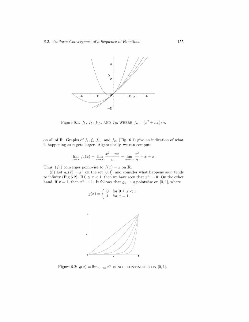
6.2. Uniform Convergence of a Sequence of Functions 155

–2

0

2

4

y

–4 –2 2 4x

Figure 6.1: f1, f5, f10, and f20 where fn = (x2 + nx)/n.

on all of R. Graphs of f1, f5, f10, and f20 (Fig. 6.1) give an indication of whatis happening as n gets larger. Algebraically, we can compute

limn→∞ fn(x) = lim

n→∞x2 + nx

n= lim

n→∞x2

n+ x = x.

Thus, (fn) converges pointwise to f(x) = x on R.(ii) Let gn(x) = xn on the set [0, 1], and consider what happens as n tends

to infinity (Fig 6.2). If 0 ≤ x < 1, then we have seen that xn → 0. On the otherhand, if x = 1, then xn → 1. It follows that gn → g pointwise on [0, 1], where

g(x) ={0 for 0 ≤ x < 11 for x = 1.

0

1

y

1x

Figure 6.2: g(x) = limn→∞ xn is not continuous on [0, 1].


–1 1x

Figure 6.3: hn → |x| on [−1, 1]; limit is not differentiable.

(iii) Consider hn(x) = x1+ 12n−1 on the set [−1, 1] (Fig. 6.3). For a fixed

x ∈ [−1, 1] we have

limn→∞hn(x) = x lim

n→∞x1

2n−1 = |x|.

Examples 6.2.2 (ii) and (iii) are our first indication that there is some difficultwork ahead of us. The central theme of this chapter is analyzing which prop-erties the limit function inherits from the approximating sequence. In Example6.2.2 (iii) we have a sequence of differentiable functions converging pointwiseto a limit that is not differentiable at the origin. In Example 6.2.2 (ii), wesee an even more fundamental problem of a sequence of continuous functionsconverging to a limit that is not continuous.

Continuity of the Limit Function

With Example 6.2.2 (ii) firmly in mind, we begin this discussion with a doomedattempt to prove that the pointwise limit of continuous functions is continuous.Upon discovering the problem in the argument, we will be in a better positionto understand the need for a stronger notion of convergence for sequences offunctions.

Assume (fn) is a sequence of continuous functions on a set A ⊆ R, andassume (fn) converges pointwise to a limit f . To argue that f is continuous, fixa point c ∈ A, and let ε > 0. We need to find a δ > 0 such that

|x− c| < δ implies |f(x)− f(c)| < δ.

By the triangle inequality,

|f(x)− f(c)| = |f(x)− fn(x) + fn(x)− fn(c) + fn(c)− f(c)|≤ |f(x)− fn(x)|+ |fn(x)− fn(c)|+ |fn(c)− f(c)|.


(We should really call this the “quadralateral inequality” because we are usingthree joined “sides” as an overestimate for the length of the fourth.) Our first,optimistic impression is that each term in the sum on the right-hand side canbe made small—the first and third by the fact that fn → f , and the middleterm by the continuity of fn. In order to use the continuity of fn, we mustfirst establish which particular fn we are talking about. Because c ∈ A is fixed,choose N ∈ N so that

|fN (c)− f(c)| < ε

3.

Now that N is chosen, the continuity of fN implies that there exists a δ > 0such that

|fN (x)− fN (c)| < ε

3

for all x satisfying |x− c| < δ.But here is the problem. We also need

|fN (x)− f(x)| < ε

3for all |x− c| < δ.

The values of x depend on δ, which depends on the choice of N . Thus, we cannotgo back and simply choose a different N . More to the point, the variable x isnot fixed the way c is in this discussion but represents any point in the interval(c−δ, c+δ). Pointwise convergence implies that we can make |fn(x)−f(x)| < ε/3for large enough values of n, but the value of n depends on the point x. It ispossible that different values for x will result in the need for different—larger—choices for n. This phenomenon is apparent in Example 6.2.2 (ii). To achievethe inequality

|gn(1/2)− g(1/2)| < 13,

we need n ≥ 2, whereas

|gn(9/10)− g(9/10)| < 13

is true only after n ≥ 11.

Uniform Convergence

To resolve this dilemma, we define a new, stronger notion of convergence offunctions.

Definition 6.2.3. Let fn be a sequence of functions defined on a set A ⊆ R.Then, (fn) converges uniformly on A to a limit function f defined on A if, forevery ε > 0, there exists an N ∈ N such that |fn(x)−f(x)| < ε whenever n ≥ Nand x ∈ A.

To emphasize the difference between uniform convergence and pointwise con-vergence, we restate Definition 6.2.1, being more explicit about the relationship


between ε,N , and x. In particular, notice where the domain point x is refer-enced in each definition and consequently how the choice of N then does or doesnot depend on this value.

Definition 6.2.1B. Let fn be a sequence of functions defined on a set A ⊆ R.Then, (fn) converges pointwise on A to a limit f defined on A if, for everyε > 0 and x ∈ A, there exists an N ∈ N (perhaps dependent on x) such that|fn(x)− f(x)| < ε whenever n ≥ N .

The use of the adverb uniformly here should be reminiscent of its use inthe phrase “uniformly continuous” from Chapter 4. In both cases, the term“uniformly” is employed to express the fact that the response (δ or N) to aprescribed ε can be chosen to work simultaneously for all values of x in therelevant domain.

Example 6.2.4. (i) Let

gn(x) =1

n(1 + x2).

For any fixed x ∈ R, we can see that lim gn(x) = 0 so that g(x) = 0 is thepointwise limit of the sequence (gn) on R. Is this convergence uniform? Theobservation that 1/(1 + x2) ≤ 1 for all x ∈ R implies that

|gn(x)− g(x)| =∣∣∣∣ 1n(1 + x2)

− 0∣∣∣∣ ≤ 1

n.

Thus, given ε > 0, we can choose N > 1/ε (which does not depend on x), andit follows that

n ≥ N implies |gn(x)− g(x)| < ε

for all x ∈ R. By Definition 6.2.3, gn → 0 uniformly on R.

(ii) Look back at Example 6.2.2 (i), where we saw that fn(x) = (x2+nx)/nconverges pointwise on R to f(x) = x. On R, the convergence is not uniform.To see this write

|fn(x)− f(x)| =∣∣∣∣x2 + nx

n− x

∣∣∣∣ = x2

n,

and notice that in order to force |fn(x) − f(x)| < ε, we are going to have tochoose

N >x2

ε.

Although this is possible to do for each x ∈ R, there is no way to choose a singlevalue of N that will work for all values of x at the same time.

On the other hand, we can show that fn → f uniformly on the set [−b, b].By restricting our attention to a bounded interval, we may now assert that

x2

n≤ b2

n.


✲︸︷︷︸A

�✠

fn,n≥Nf+ε

f

f−ε

Figure 6.4: fn → f uniformly on A.

︸︷︷︸A

g1g2g3g4

g+ε

g

g−ε

Figure 6.5: gn → g pointwise, but not uniformly.

Given ε > 0, then, we can choose

N >b2

ε

independently of x ∈ [−b, b].

Graphically speaking, the uniform convergence of fn to a limit f on a set Acan be visualized by constructing a band of radius ±ε around the limit functionf . If fn → f uniformly, then there exists a point in the sequence after whicheach fn is completely contained in this ε-strip (Fig. 6.4). This image should becompared with the graphs in Figures 6.1–6.2 from Example 6.2.2 and the onein Figure 6.5.

Cauchy Criterion

Recall that the Cauchy Criterion for convergent sequences of real numbers wasan equivalent characterization of convergence which, unlike the definition, didnot make explicit mention of the limit. The usefulness of the Cauchy Criterionsuggests the need for an analogous characterization of uniformly convergentsequences of functions. As with all statements about uniformity, pay attentionto where the quantifying phrase “for all x ∈ A” appears in the statement.


Theorem 6.2.5 (Cauchy Criterion for Uniform Convergence). A sequenceof functions (fn) defined on a set A ⊆ R converges uniformly on A if and onlyif for every ε > 0 there exists an N ∈ N such that |fn(x) − fm(x)| < ε for allm,n ≥ N and all x ∈ A.


Continuity Revisited

The stronger assumption of uniform convergence is precisely what is required toremove the flaws from our attempted proof that the limit of continuous functionsis continuous.

Theorem 6.2.6. Let (fn) be a sequence of functions defined on A ⊆ R thatconverges uniformly on A to a function f . If each fn is continuous at c ∈ A,then f is continuous at c.

Proof. Fix c ∈ A and let ε > 0. Choose N so that

|fN (x)− f(x)| < ε

3

for all x ∈ A. Because fN is continuous, there exists a δ > 0 for which

|fN (x)− fN (c)| < ε

3

is true whenever |x− c| < δ. But this implies

|f(x)− f(c)| = |f(x)− fN (x) + fN (x)− fN (c) + fN (c)− f(c)|≤ |f(x)− fN (x)|+ |fN (x)− fN (c)|+ |fN (c)− f(c)|<

ε

3+

ε

3+

ε

3= ε.

Thus, f is continuous at c ∈ A.

Exercises

Exercise 6.2.1. Letfn(x) =

nx

1 + nx2 .

(a) Find the pointwise limit of (fn) for all x ∈ (0,∞).(b) Is the convergence uniform on (0,∞)?(c) Is the convergence uniform on (0, 1)?(d) Is the convergence uniform on (1,∞)?

Exercise 6.2.2. Let

gn(x) =nx+ sin(nx)

2n.

Find the pointwise limit of (gn) on R. Is the convergence uniform on [−10, 10]?Is the convergence uniform on all of R?


Exercise 6.2.3. Consider the sequence of functions

hn(x) =x

1 + xn

over the domain [0,∞).(a) Find the pointwise limit of (hn) on [0,∞).(b) Explain how we know that the convergence cannot be uniform on [0,∞).(c) Choose a smaller set over which the convergence is uniform and supply

an argument to show that this is indeed the case.

Exercise 6.2.4. For each n ∈ N, find the points on R where the functionfn(x) = x/(1 + nx2) attains its maximum and minimum values. Use this toprove (fn) converges uniformly on R. What is the limit function?

Exercise 6.2.5. For each n ∈ N, define fn on R by

fn(x) ={1 if |x| ≥ 1/nn|x| if |x| < 1/n.

(a) Find the pointwise limit of (fn) on R and decide whether or not theconvergence is uniform.

(b) Construct an example of a pointwise limit of continuous functions thatconverges everywhere on the compact set [−5, 5] to a limit function that isunbounded on this set.

Exercise 6.2.6. Using the Cauchy Criterion for convergent sequences of realnumbers (Theorem 2.6.4), supply a proof for Theorem 6.2.5. (First, define acandidate for f(x), and then argue that fn → f uniformly.)

Exercise 6.2.7. Assume that (fn) converges uniformly to f on A and that eachfn is uniformly continuous on A. Prove that f is uniformly continuous on A.

Exercise 6.2.8. Decide which of the following conjectures are true and whichare false. Supply a proof for those that are valid and a counterexample for eachone that is not.

(a) If fn → f pointwise on a compact set K, then fn → f uniformly on K.(b) If fn → f uniformly on A and g is a bounded function on A, then

fng → fg uniformly on A.(c) If fn → f uniformly on A, and if each fn is bounded on A, then f must

also be bounded.(d) If fn → f uniformly on a set A, and if fn → f uniformly on a set B,

then fn → f uniformly on A ∪B.(e) If fn → f uniformly on an interval, and if each fn is increasing, then f

is also increasing.(f) Repeat conjecture (e) assuming only pointwise convergence.

Exercise 6.2.9. Assume (fn) converges uniformly to f on a compact set K,and let g be a continuous function on K satisfying g(x) �= 0. Show (fn/g)converges uniformly on K to f/g.


Exercise 6.2.10. Let f be uniformly continuous on all of R, and define asequence of functions by fn(x) = f(x + 1

n ). Show that fn → f uniformly.Give an example to show that this proposition fails if f is only assumed to becontinuous and not uniformly continuous on R.

Exercise 6.2.11. Assume (fn) and (gn) are uniformly convergent sequences offunctions.

(a) Show that (fn + gn) is a uniformly convergent sequence of functions.(b) Give an example to show that the product (fngn) may not converge

uniformly.(c) Prove that if there exists an M > 0 such that |fn| ≤ M and |gn| ≤ M

for all n ∈ N, then (fngn) does converge uniformly.

Exercise 6.2.12. Theorem 6.2.6 has a partial converse. Assume fn → f point-wise on a compact set K and assume that for each x ∈ K the sequence fn(x)is increasing. Follow these steps to show that if fn and f are continuous on K,then the convergence is uniform.

(a) Set gn = f − fn and translate the preceding hypothesis into statementsabout the sequence (gn).

(b) Let ε > 0 be arbitrary, and define Kn = {x ∈ K : gn(x) ≥ ε}. Arguethat K1 ⊇ K2 ⊇ K3 ⊇ · · · is a nested sequence of compact sets, and use thisobservation to finish the argument.

Exercise 6.2.13 (Cantor Function). Review the construction of the Cantorset C ⊆ [0, 1] from Section 3.1. This exercise makes use of results and notationfrom this discussion.

(a) Define f0(x) = x for all x ∈ [0, 1]. Now, let

f1(x) =

(3/2)x for 0 ≤ x ≤ 1/31/2 for 1/3 < x < 2/3(3/2)x− 1/2 for 2/3 ≤ x ≤ 1.

Sketch f0 and f1 over [0, 1] and observe that f1 is continuous, increasing, andconstant on the middle third (1/3, 2/3) = [0, 1]\C1.

(b) Construct f2 by imitating this process of flattening out the middle thirdof each nonconstant segment of f1. Specifically, let

f2(x) =

(1/2)f1(3x) for 0 ≤ x ≤ 1/3f1(x) for 1/3 < x < 2/3(1/2)f1(3x− 2) + 1/2 for 2/3 ≤ x ≤ 1.

If we continue this process, show that the resulting sequence (fn) convergesuniformly on [0, 1].

(c) Let f = lim fn. Prove that f is a continuous, increasing function on[0, 1] with f(0) = 0 and f(1) = 1 that satisfies f ′(x) = 0 for all x in the openset [0, 1]\C. Recall that the “length” of the Cantor set C is 0. Somehow, fmanages to increase from 0 to 1 while remaining constant on a set of “length1.”


Exercise 6.2.14. Recall that the Bolzano–Weierstrass Theorem (Theorem 2.5.5)states that every bounded sequence of real numbers has a convergent subse-quence. An analogous statement for bounded sequences of functions is not truein general, but under stronger hypotheses several different conclusions are pos-sible. One avenue is to assume the common domain for all of the functions inthe sequence is countable. (Another is explored in the next two exercises.)

Let A = {x1, x2, x3, . . . } be a countable set. For each n ∈ N, let fn be defineon A and assume there exists an M > 0 such that |fn(x)| ≤ M for all n ∈ Nand x ∈ A. Follow these steps to show that there exists a subsequence of (fn)that converges pointwise on A.

(a) Why does the sequence of real numbers fn(x1) necessarily contain aconvergent subsequence (fnk

)? To indicate that the subsequence of functions(fnk

) is generated by considering the values of the functions at x1, we will usethe notation fnk

= f1,k.(b) Now, explain why the sequence f1,k(x2) contains a bounded subsequence.(c) Carefully construct a nested family of subsequences (fm,k), and use Can-

tor’s diagonalization technique (from Theorem 1.5.1) to produce a single subse-quence of (fn) that converges at every point of A.

Exercise 6.2.15. A sequence of functions (fn) defined on a set E ⊆ R is calledequicontinuous if for every ε > 0 there exists a δ > 0 such that |fn(x)−fn(y)| < εfor all n ∈ N and |x− y| < δ in E.

(a) What is the difference between saying that a sequence of functions (fn)is equicontinuous and just asserting that each fn in the sequence is individuallyuniformly continuous?

(b) Give a qualitative explanation for why the sequence gn(x) = xn is notequicontinuous on [0, 1]. Is each gn uniformly continuous on [0, 1]?

Exercise 6.2.16 (Arzela–Ascoli Theorem). For each n ∈ N, let fn be afunction defined on [0, 1]. If (fn) is bounded on [0, 1]—that is, there exists anM > 0 such that |fn(x)| ≤ M for all n ∈ N and x ∈ [0, 1]—and if the collectionof functions (fn) is equicontinuous (Exercise 6.2.15), follow these steps to showthat (fn) contains a uniformly convergent subsequence.

(a) Use Exercise 6.2.14 to produce a subsequence (fnk) that converges at

every rational point in [0, 1]. To simplify the notation, set gk = fnk. It remains

to show that (gk) converges uniformly on all of [0, 1].(b) Let ε > 0. By equicontinuity, there exists a δ > 0 such that

|gk(x)− gk(y)| < ε

3

for all |x−y| < δ and k ∈ N. Using this δ, let r1, r2, . . . , rm be a finite collectionof rational points with the property that the union of the neighborhoods Vδ(ri)contains [0,1].

Explain why there must exist an N ∈ N such that

|gs(ri)− gt(ri)| < ε

3


for all s, t ≥ N and ri in the finite subset of [0, 1] just described. Why doeshaving the set {r1, r2, . . . , rm} be finite matter?

(c) Finish the argument by showing that, for an arbitrary x ∈ [0, 1],|gs(x)− gt(x)| < ε

for all s, t ≥ N .

6.3 Uniform Convergence and Differentiation

Example 6.2.2 (iii) imposes some significant restrictions on what we might hopeto be true regarding differentiation and uniform convergence. If hn → h uni-formly and each hn is differentiable, we should not anticipate that h′

n → h′

because in this example h′(x) does not even exist at x = 0.The key assumption necessary to be able to prove any facts about the deriva-

tive of the limit function is that the sequence of derivatives be uniformly con-vergent. This may sound as though we are assuming what it is we would liketo prove, and there is some validity to this complaint. The more hypothesesa proposition has, the more difficult it is to apply. The content of the nexttheorem is that if we are given a pointwise convergent sequence of differentiablefunctions, and if we know that the sequence of derivatives converges uniformlyto something, then the limit of the derivatives is indeed the derivative of thelimit.

Theorem 6.3.1. Let fn → f pointwise on the closed interval [a, b], and assumethat each fn is differentiable. If (f ′

n) converges uniformly on [a, b] to a functiong, then the function f is differentiable and f ′ = g.

Proof. Let ε > 0 and fix c ∈ [a, b]. We want to argue that f ′(c) exists and equalsg(c). Because f ′ is defined by the limit

f ′(c) = limx→c

f(x)− f(c)x− c

,

our task is to produce a δ > 0 so that∣∣∣∣f(x)− f(c)x− c

− g(c)∣∣∣∣ < ε

whenever 0 < |x− c| < δ. Using the triangle inequality, we can estimate

∣∣∣∣f(x)− f(c)x− c

− g(c)∣∣∣∣ ≤

∣∣∣∣f(x)− f(c)x− c

− fn(x)− fn(c)x− c

∣∣∣∣+∣∣∣∣fn(x)− fn(c)

x− c− f ′

n(c)∣∣∣∣+ |f ′

n(c)− g(c)| .

Our intent is to force each of the three terms on the right-hand side to be lessthan ε/3. This will not be too difficult in the case of the third term (because

6.3. Uniform Convergence and Differentiation 165

f ′n → g uniformly) nor in the case of the second (because f ′

n is differentiable).Handling the first term requires the most delicate touch, and we tend to thistask first.

Apply the Mean Value Theorem to the function fm−fn on the interval [c, x].(If x < c, the argument is the same.) By MVT, there exists an α ∈ (c, x) suchthat

f ′m(α)− f ′

n(α) =(fm(x)− fn(x))− (fm(c)− fn(c))

x− c.

Now, by the Cauchy Criterion for Uniform Convergence (Theorem 6.2.5), thereexists an N1 ∈ N such that m,n ≥ N1 implies

|f ′m(α)− f ′

n(α)| <ε

3.

We should point out that α depends on the choice of m and n, so it is crucial tohave uniform convergence of (f ′

n) at this point in the argument. Putting theselast two statements together leads to the conclusion that∣∣∣∣fm(x)− fm(c)

x− c− fn(x)− fn(c)

x− c

∣∣∣∣ < ε

3

for all m,n ≥ N1 and all x ∈ [a, b]. Because fm → f , we can take the limit asm → ∞ and use the Order Limit Theorem (Theorem 2.3.4) to assert that∣∣∣∣f(x)− f(c)

x− c− fn(x)− fn(c)

x− c

∣∣∣∣ ≤ ε

3

for all n ≥ N1.To complete the proof, choose N2 large enough so that

|f ′m(c)− g(c)| < ε

3

for all m ≥ N2, and then let N = max{N1, N2}. Having settled on a choice ofN , we use the fact that fN is differentiable to produce a δ > 0 for which∣∣∣∣fN (x)− fN (c)

x− c− f ′

N (c)∣∣∣∣ < ε

3

whenever 0 < |x− c| < δ. Finally, we observe that for these values of x,∣∣∣∣f(x)− f(c)x− c

− g(c)∣∣∣∣ ≤

∣∣∣∣f(x)− f(c)x− c

− fN (x)− fN (c)x− c

∣∣∣∣+∣∣∣∣fN (x)− fN (c)

x− c− f ′

N (c)∣∣∣∣+ |f ′

N (c)− g(c)|

<ε

3+

ε

3+

ε

3= ε


The hypothesis in Theorem 6.3.1 is unnecessarily strong. We actually donot need to assume that fn(x)→ f(x) at each point in the domain because theassumption that the sequence of derivatives (f ′

n) converges uniformly is nearlystrong enough to prove that (fn) converges, uniformly in fact. Two functionswith the same derivative may differ by a constant, so we must assume that thereis at least one point x0 where fn(x0)→ f(x0).

Theorem 6.3.2. Let (fn) be a sequence of differentiable functions defined onthe closed interval [a, b], and assume (f ′

n) converges uniformly on [a, b]. If thereexists a point x0 ∈ [a, b] where fn(x0) is convergent, then (fn) converges uni-formly on [a, b].


Combining the last two results produces a stronger version of Theorem 6.3.1.

Theorem 6.3.3. Let (fn) be a sequence of differentiable functions defined onthe closed interval [a, b], and assume (f ′

n) converges uniformly to a function g on[a, b]. If there exists a point x0 ∈ [a, b] for which fn(x0) is convergent, then (fn)converges uniformly. Moreover, the limit function f = lim fn is differentiableand satisfies f ′ = g.

Exercises

Exercise 6.3.1. (a) Let

hn(x) =sin(nx)

n.

Show that hn → 0 uniformly on R. At what points does the sequence ofderivatives h′

n converge?(b) Modify this example to show that it is possible for a sequence (fn) to

converge uniformly but for (f ′n) to be unbounded.

Exercise 6.3.2. Consider the sequence of functions defined by

gn(x) =xn

n.

(a) Show (gn) converges uniformly on [0, 1] and find g = lim gn. Show thatg is differentiable and compute g′(x) for all x ∈ [0, 1].

(b) Now, show that (g′n) converges on [0, 1]. Is the convergence uniform?Set h = lim g′n and compare h and g′. Are they the same?

Exercise 6.3.3. Consider the sequence of functions

fn(x) =x

1 + nx2 .

Exercise 6.2.4 contains some advice for how to show that (fn) converges uni-formly on R. Review or complete this exercise.

Now, let f = lim fn. Compute f ′n(x) and find all the values of x for which

f ′(x) = lim f ′n(x).

6.4. Series of Functions 167

Exercise 6.3.4. Let

gn(x) =nx+ x2

2n,

and set g(x) = lim gn(x). Show that g is differentiable in two ways:(a) Compute g(x) by algebraically taking the limit as n → ∞ and then find

g′(x).(b) Compute g′n(x) for each n ∈ N and show that the sequence of derivatives

(g′n) converges uniformly on every interval [−M,M ]. Use Theorem 6.3.3 toconclude g′(x) = lim g′n(x).

(c) Repeat parts (a) and (b) for the sequence fn(x) = (nx2 + 1)/(2n+ x).

Exercise 6.3.5. Use the following advice to supply a proof for Theorem 6.3.2.To get started, observe that the triangle inequality implies that, for any x ∈[a, b],

|fn(x)− fm(x)| ≤ |(fn(x)− fm(x))− (fn(x0)− fm(x0))|+ |fn(x0)− fm(x0)|.Now, apply the Mean Value Theorem to fn − fm.

6.4 Series of Functions

Definition 6.4.1. For each n ∈ N, let fn and f be functions defined on a setA ⊆ R. The infinite series

∞∑n=1

fn(x) = f1(x) + f2(x) + f3(x) + · · ·

converges pointwise on A to f(x) if the sequence sk(x) of partial sums definedby

sk(x) = f1(x) + f2(x) + · · ·+ fk(x)

converges pointwise to f(x). The series converges uniformly on A to f if thesequence sk(x) converges uniformly on A to f(x).

In either case, we write f =∑∞

n=1 fn or f(x) =∑∞

n=1 fn(x), always beingexplicit about the type of convergence involved.

If we have a series∑∞

n=1 fn where the functions fn are continuous, thenthe Algebraic Continuity Theorem (Theorem 4.3.4) guarantees that the partialsums—because they are finite sums—will be continuous as well. A correspond-ing observation is true if we are dealing with differentiable functions. As aconsequence, we can immediately translate the results for sequences in the pre-vious sections into statements about the behavior of infinite series of functions.

Theorem 6.4.2. Let fn be continuous functions defined on a set A ⊆ R, andassume

∑∞n=1 fn converges uniformly on A to a function f . Then, f is contin-

uous on A.

Proof. Apply Theorem 6.2.6 to the partial sums sk = f1 + f2 + · · ·+ fk.


Theorem 6.4.3. Let fn be differentiable functions defined on an interval [a, b],and assume

∑∞n=1 f

′n(x) converges uniformly to a limit g(x) on A. If there exists

a point x0 ∈ [a, b] where∑∞

n=1 fn(x0) converges, then the series∑∞

n=1 fn(x)converges uniformly to a differentiable function f(x) satisfying f ′(x) = g(x) on[a, b]. In other words,

f(x) =∞∑n=1

fn(x) and f ′(x) =∞∑n=1

f ′n(x).

Proof. Apply Theorem 6.3.3 to the partial sums sk = f1+f2+ · · ·+fk. Observethat Theorem 5.2.4 implies that s′k = f ′

1 + f ′2 + · · ·+ f ′

k.

In the vocabulary of infinite series, the Cauchy Criterion takes the followingform.

Theorem 6.4.4 (Cauchy Criterion for Uniform Convergence of Series).A series

∑∞n=1 fn converges uniformly on A ⊆ R if and only if for every ε > 0

there exists an N ∈ N such that for all n > m ≥ N ,

|fm+1(x) + fm+2(x) + fm+3(x) + · · ·+ fn(x)| < ε

for all x ∈ A.

The benefits of uniform convergence over pointwise convergence suggest theneed for some ways of determining when a series converges uniformly. Thefollowing corollary to the Cauchy Criterion is the most common such tool. Inparticular, it will be quite useful in our upcoming investigations of power series.

Corollary 6.4.5 (Weierstrass M-Test). For each n ∈ N, let fn be a func-tion defined on a set A ⊆ R, and let Mn > 0 be a real number satisfying

|fn(x)| ≤ Mn

for all x ∈ A. If∑∞

n=1 Mn converges, then∑∞

n=1 fn converges uniformly on A.


Exercises

Exercise 6.4.1. Prove that if∑∞

n=1 gn converges uniformly, then (gn) con-verges uniformly to zero.

Exercise 6.4.2. Supply the details for the proof of the Weierstrass M-Test(Corollary 6.4.5).

Exercise 6.4.3. (a) Show that g(x) =∑∞

n=1 cos(2nx)/2n is continuous on all

of R.(b) Prove that h(x) =

∑∞n=1 x

n/n2 is continuous on [−1, 1].

6.5. Power Series 169

Exercise 6.4.4. In Section 5.4, we postponed the argument that the nowhere-differentiable function

g(x) =∞∑n=0

12n

h(2nx)

is continuous on R. Use the Weierstrass M-Test to supply the missing proof.

Exercise 6.4.5. Let

f(x) =∞∑k=1

sin(kx)k3 .

(a) Show that f(x) is differentiable and that the derivative f ′(x) is contin-uous.

(b) Can we determine if f is twice-differentiable?

Exercise 6.4.6. Observe that the series

f(x) =∞∑n=1

xn

n= x+

x2

2+

x3

3+

x4

4+ · · ·

converges for every x in the half-open interval [0, 1) but does not converge whenx = 1. For a fixed x0 ∈ (0, 1), explain how we can still use the WeierstrassM-Test to prove that f is continuous at x0.

Exercise 6.4.7. Let

h(x) =∞∑n=1

1x2 + n2 .

(a) Show that h is a continuous function defined on all of R.(b) Is h differentiable? If so, is the derivative function h′ continuous?

Exercise 6.4.8. Let {r1, r2, r3, . . . } be an enumeration of the set of rationalnumbers. For each rn ∈ Q, define

un(x) ={1/2n for x > rn0 for x ≤ rn.

Now, let h(x) =∑∞

n=1 un(x). Prove that h is a monotone function defined onall of R that is continuous at every irrational point.

6.5 Power Series

It is time to put some mathematical teeth into our understanding of functionsexpressed in the form of a power series; that is, functions of the form

f(x) =∞∑n=0


2 + a3x3 + · · · .

The first order of business is to determine the points x ∈ R for which theresulting series on the right-hand side converges. This set certainly containsx = 0, and, as the next result demonstrates, it takes a very predictable form.


Theorem 6.5.1. If a power series∑∞

n=0 anxn converges at some point x0 ∈ R,

then it converges absolutely for any x satisfying |x| < |x0|.Proof. If

∑∞n=0 anx

n0 converges, then the sequence of terms (anx

n0 ) is bounded.

(In fact, it converges to 0.) Let M > 0 satisfy |anxn0 | ≤ M for all n ∈ N. Ifx ∈ R satisfies |x| < |x0|, then

|anxn| = |anx0|n∣∣∣∣ xx0

∣∣∣∣n ≤ M

∣∣∣∣ xx0

∣∣∣∣n .

But notice that ∞∑n=0

M

∣∣∣∣ xx0

∣∣∣∣nis a geometric series with ratio |x/x0| < 1 and so converges. By the ComparisonTest,

∑∞n=0 anx

n converges absolutely.

The main implication of Theorem 6.5.1 is that the set of points for which agiven power series converges must necessarily be {0}, R, or a bounded intervalcentered around x = 0. Because of the strict inequality in Theorem 6.5.1, thereis some ambiguity about the endpoints of the interval, and it is possible thatthe set of convergent points may be of the form (−R,R), [−R,R), (−R,R], or[−R,R].

The value of R is referred to as the radius of convergence of a power series,and it is customary to assign R the value 0 or ∞ to represent the set {0}or R, respectively. Some of the standard devices for computing the radius ofconvergence for a power series are explored in the exercises. Of more interestto us here is the investigation of the properties of functions defined in this way.Are they continuous? Are they differentiable? If so, can we differentiate theseries term-by-term? What happens at the endpoints?

Establishing Uniform Convergence

The positive answers to the preceding questions, and the usefulness of powerseries in general, are largely due to the fact that they converge uniformly oncompact sets contained in their domain of convergent points. As we are about tosee, a complete proof of this fact requires a fairly delicate argument attributedto the Norwegian mathematician Niels Abel. A significant amount of progress,however, can be made with the Weierstrass M-Test (Corollary 6.4.5).

Theorem 6.5.2. If a power series∑∞

n=0 anxn converges absolutely at a point

x0, then it converges uniformly on the closed interval [−c, c], where c = |x0|.Proof. This proof requires a straightforward application of the Weierstrass M-Test. The details are requested in Exercise 6.5.5.

For many applications, Theorem 6.5.2 is good enough. For instance, com-bining our results about uniform convergence and power series to this point, we


can now argue that a power series that converges on an open interval (−R,R)is necessarily continuous on this interval (Exercise 6.5.4).

But what happens if we know that a series converges at an endpoint ofits interval of convergence? Does the good behavior of the series on (−R,R)necessarily extend to the endpoint x = R? If the convergence of the series atx = R is absolute convergence, then we can again rely on Theorem 6.5.2 toconclude that the series converges uniformly on the set [−R,R]. The remaininginteresting open question is what happens if a series converges conditionallyat a point x = R. We may still use Theorem 6.5.1 to conclude that we havepointwise convergence on the interval (−R,R], but more work is needed toestablish uniform convergence on compact sets containing x = R.

Abel’s Theorem

We should remark that if the power series g(x) =∑∞

n=0 anxn converges con-

ditionally at x = R, then it is possible for it to diverge when x = −R. Theseries ∞∑

n=1

(−1)nxnn

with R = 1 is an example. To keep our attention fixed on the convergentendpoint, we will prove uniform convergence on the set [0, R].

The argument we need is very similar to the proof of Abel’s Test, which isincluded in the exercises of Section 2.7. The first step in the proof of Abel’sTest is an estimate, sometimes called Abel’s Lemma, which we will presentlyneed again.

Lemma 6.5.3 (Abel’s Lemma). Let bn satisfy b1 ≥ b2 ≥ b3 ≥ · · · ≥ 0, andlet∑∞

n=1 an be a series for which the partial sums are bounded. In other words,assume there exists A > 0 such that

|a1 + a2 + · · ·+ an| ≤ A

for all n ∈ N . Then, for all n ∈ N,

|a1b1 + a2b2 + a3b3 + · · ·+ anbn| ≤ 2Ab1.

Proof. This inequality follows from the so-called summation-by-parts formula.Exercises 2.7.12 and 2.7.14(b) from Section 2.7 contain the relevant definitionsand advice required to complete the argument.

It is worth observing that if A were an upper bound on the partial sumsof∑ |an| (note the absolute value bars), then the proof of Lemma 6.5.3 would

be a simple exercise in the triangle inequality. (Also, we would not need thefactor of 2, and, actually, it is not needed in general except that our particularmethod of proof requires it.) The point of the matter is that because we areonly assuming conditional convergence, the triangle inequality is not going tobe of any use in proving Abel’s Theorem, but we are now in possession of aninequality that we can use in its place.


Theorem 6.5.4 (Abel’s Theorem). Let g(x) =∑∞

n=0 anxn be a power se-

ries that converges at the point x = R > 0. Then the series converges uniformlyon the interval [0, R]. A similar result holds if the series converges at x = −R.

Proof. To set the stage for an application of Lemma 6.5.3, we first write

g(x) =∞∑n=0

anxn =

∞∑n=0

(anRn)( x

R

)n.

Let ε > 0. By the Cauchy Criterion for Uniform Convergence of Series (Theo-rem 6.4.4), we will be done if we can produce an N such that n > m ≥ N implies

(1)∣∣∣∣(am+1R

m+1)( x

R

)m+1+ (am+2R

m+2)( x

R

)m+2+ · · ·

+(anRn)( x

R

)n∣∣∣ < ε.

Because we are assuming that∑∞

n=1 anRn converges, the Cauchy Criterion for

convergent series of real numbers guarantees that there exists an N such that

|am+1Rm+1 + am+2R

m+2 + · · ·+ anRn| < ε

2

whenever n > m ≥ N . But now, for any fixed m ∈ N , we can apply Lemma6.5.3 to the sequences obtained by omitting the first m terms. Using ε/2 as abound on the partial sums of

∑∞j=1 am+jR

m+j and observing that (x/R)m+j ismonotone decreasing, an application of Lemma 6.5.3 to equation (1) yields

∣∣∣∣(am+1Rm+1)

( x

R

)m+1+ (am+2R

m+2)( x

R

)m+2+ · · ·

+ (anRn)( x

R

)n∣∣∣ ≤ 2( ε2

)( x

R

)m+1≤ ε.

The fact that the inequality is not strict (as the Cauchy Criterion technicallyrequires) is a distraction but not a real deficiency. We leave it as a point fordiscussion.

The Success of Power Series

An economical way to summarize the conclusions of Theorem 6.5.2 and Abel’sTheorem is with the following statement.

Theorem 6.5.5. If a power series converges pointwise on the set A ⊆ R, thenit converges uniformly on any compact set K ⊆ A.



This fact leads to the desirable conclusion that a power series is continuousat every point at which it converges. To make an argument for differentia-bility, we would like to appeal to Theorem 6.4.3; however, this result has aslightly more involved set of hypotheses. In order to conclude that a powerseries

∑∞n=0 anx

n is differentiable, and that term-by-term differentiation is al-lowed, we need to know beforehand that the differentiated series

∑∞n=1 nanx

n−1

converges uniformly.

Theorem 6.5.6. If∑∞

n=0 anxn converges for all x ∈ (−R,R), then the differ-

entiated series∑∞

n=1 nanxn−1 converges at each x ∈ (−R,R) as well. Conse-

quently, the convergence is uniform on compact sets contained in (−R,R).


We should point out that it is possible for a series to converge at an end-point x = R but for the differentiated series to diverge at this point. The series∑∞

n=1(−x)n/n has this property when x = 1. On the other hand, if the differ-entiated series does converge at the point x = R, then Abel’s Theorem appliesand the convergence of the differentiated series is uniform on compact sets thatcontain R.

With all the pieces in place, we summarize the impressive conclusions of thissection.

Theorem 6.5.7. Assume

g(x) =∞∑n=0

anxn

converges on an interval A ⊆ R. The function g is continuous on A and differ-entiable on any open interval (−R,R) ⊆ A. The derivative is given by

g′(x) =∞∑n=1

nanxn−1.

Moreover, g is infinitely differentiable on (−R,R), and the successive derivativescan be obtained via term-by-term differentiation of the appropriate series.

Proof. The details for why g is continuous are requested in the exercises. The-orem 6.5.6 justifies the application of Theorem 6.4.3, which verifies the formulafor g′.

A differentiated power series is a power series in its own right, and Theorem6.5.6 implies that, although the series may no longer converge at a particularendpoint, the radius of convergence does not change. By induction, then, powerseries are differentiable an infinite number of times.


Exercises

Exercise 6.5.1. Consider the function g defined by the power series

g(x) = x− x2

2+

x3

3− x4

4+

x5

5− · · · .

(a) Is g defined on (−1, 1)? Is it continuous on this set? Is g defined on(−1, 1]? Is it continuous on this set? What happens on [−1, 1]? Can the powerseries for g(x) possibly converge for any other points |x| > 1? Explain.

(b) For what values of x is g′(x) defined? Find a formula for g′.

Exercise 6.5.2. Find suitable coefficients (an) so that the resulting power se-ries

∑anx

n

(a) converges absolutely for all x ∈ [−1, 1] and diverges off of this set;(b) converges conditionally at x = −1 and diverges at x = 1;(c) converges conditionally at both x = −1 and x = 1.(d) Is it possible to find an example of a power series that converges condi-

tionally at x = −1 and converges absolutely at x = 1?

Exercise 6.5.3. Explain why a power series can converge conditionally for atmost two points.

Exercise 6.5.4. (a) By referencing the proper theorems, produce a detailedargument that a power series that converges on the interval (−R,R) necessarilyrepresents a continuous function at each point x ∈ (−R,R).

(b) If the series converges at an endpoint x = R, point out how we knowcontinuity extends to the set (R,R].

Exercise 6.5.5. Use the Weierstrass M-Test to prove Theorem 6.5.2.

Exercise 6.5.6. Show how Theorem 6.5.1, Theorem 6.5.2, and Abel’s Theoremtogether imply that if a power series converges pointwise on a compact set, thenthe convergence is actually uniform on this set.

Exercise 6.5.7. (a) The Ratio Test (from Exercise 2.7.9) states that if (bn) isa sequence of nonzero terms satisfying lim |bn+1/bn| = r < 1, then the series∑

bn converges. Use this to argue that if s satisfies 0 < s < 1, then nsn−1 isbounded for all n ≥ 1.

(b) Given an arbitrary x ∈ (−R,R), pick t to satisfy |x| < t < R. Use theobservation

|nanxn−1| = 1t

(n

∣∣∣∣xn−1

tn−1

∣∣∣∣)|antn|

to construct a proof for Theorem 6.5.6.

Exercise 6.5.8. Let∑

anxn be a power series with an �= 0, and assume

L = limn→∞

∣∣∣∣an+1

an

∣∣∣∣


exists.(a) Show that if L �= 0, then the series converges for all x in (−1/L, 1/L).

(The advice in Exercise 2.7.9 may be helpful.)(b) Show that if L = 0, then the series converges for all x ∈ R.(c) Show that (a) and (b) continue to hold if L is replaced by the limit

L′ = limn→∞ sn where sn = sup

{∣∣∣∣ak+1

ak

∣∣∣∣ : k ≥ n

}.

The value L′ is called the “limit superior” or “lim sup” of the sequence |an+1/an|.It exists if and only if the sequence is bounded (Exercise 2.4.6).

(d) Show that if |an+1/an| is unbounded, then the original series∑

anxn

converges only when x = 0.

Exercise 6.5.9. Use Theorem 6.5.7 to argue that power series are unique. Ifwe have ∞∑

n=0

anxn =

∞∑n=0

bnxn

for all x in an interval (−R,R), prove that an = bn for all n = 0, 1, 2, . . . . (Startby showing that a0 = b0.)

Exercise 6.5.10. Review the definitions and results from Section 2.8 concern-ing products of series and Cauchy products in particular. At the end of Section2.9, we mentioned the following result: If both

∑an and

∑bn converge condi-

tionally to A and B respectively, then it is possible for the Cauchy product,∑dn where dn = a0bn + a1bn−1 + · · ·+ anb0,

to diverge. However, if∑

dn does converge, then it must converge to AB. Toprove this, set

f(x) =∑

anxn, g(x) =

∑bnx

n, and h(x) =∑

dnxn.

Use Abel’s Theorem and the result in Exercise 2.8.8 to establish this result.

Exercise 6.5.11. A series∑∞

n=0 an is said to be Abel-summable to L if thepower series

f(x) =∞∑n=0

anxn

converges for all x ∈ [0, 1) and L = limx→1− f(x).(a) Show that any series that converges to a limit L is also Abel-summable

to L.(b) Show that

∑∞n=0(−1)n is Abel-summable and find the sum.

Exercise 6.5.12. Consider the function G from the opening discussion onbranching processes, and recall that the increasing monotone sequence of prob-abilities (dr) has a limit d = lim dr that satisfies G(d) = d. Assume we are inthe situation where there are two fixed points: G(1) = 1 and some other value0 < d0 < 1 satisfying G(d0) = d0. Formulate an argument for why the sequence(dr) necessarily converges to the value d = d0 and not to d = 1.


6.6 Taylor Series

Our study of power series has led to some enthusiastic conclusions about thenature of functions of the form

f(x) = a0 + a1x+ a2x2 + a3x

3 + a4x4 + · · · .

Despite their infinite character, power series can be manipulated more or lessas though they are polynomials. On its interval of convergence, a power se-ries is continuous and infinitely differentiable, and successive derivatives can becomputed by performing the desired operation on each individual term in theseries—just as it is done for polynomials. As we will see in the next chapter,the situation regarding integrals of power series is just as pleasant. As studentsof introductory calculus know well, the processes of integration and differentia-tion, as well as basic algebraic manipulations, are rather straightforward whenapplied only to polynomials. It is the introduction of functions such as sin(x),ln(x), and arctan(x) that necessitates much of the symbolic acrobatics taughtin first and second semester calculus courses. This phenomenon leads us to askwhether functions such as arctan(x) and the rest have representations as powerseries.

In the examples in this section, we will assume all of the familiar properties ofthe trigonometric, inverse trigonometric, exponential, and logarithmic functions.Rigorously defining these functions is an interesting exercise in analysis. In fact,one of the most common methods for providing definitions is through powerseries. The point of this discussion, however, is to come at this question fromthe other direction. Assuming we are in possession of an infinitely differentiablefunction such as arctan(x), can we find suitable coefficients an so that

arctan(x) = a0 + a1x+ a2x2 + a3x

3 + a4x4 + · · ·

for at least some nonzero values of x?

Manipulating Series

We already have one example of a power series expansion of a familiar function.In the material on infinite series in Example 2.7.5 from Chapter 2, we provedthat

(1)1

1− t= 1 + t+ t2 + t3 + t4 + · · ·

for all t ∈ (−1, 1). Substituting −t2 for t yields

11 + t2

= 1− t2 + t4 − t6 + t8 − · · · .

But now we can use the fact that

arctan(x) =∫ x

0

11 + t2

dt.

6.6. Taylor Series 177

Although integration has not been rigorously studied at this point, we will seein Chapter 7 that if fn → f uniformly on an interval [a, b], then

∫ bafn → ∫ b

af .

This observation, together with the Fundamental Theorem of Calculus, leads tothe formula

arctan(x) = x− 13x3 +

15x5 − 1

7x7 + · · · .

Exercise 6.6.1. Upcoming results in Chapter 7 will justify this equation for allx ∈ (−1, 1), but notice that this series actually converges when x = 1. Assumingthat arctan(x) is continuous, explain why the value of the series at x = 1 mustnecessarily be arctan(1). What interesting identity do we get in this case?

Exercise 6.6.2. Starting from the identity in equation (1) of this section, find apower series representation for ln(1+x). For which values of x is this expressionvalid?

Taylor’s Formula for the Coefficients

Manipulating old series to produce new ones was a well-honed craft in the 17thand 18th centuries when the usefulness of infinite series was first being realized.But there also emerged a formula for producing the coefficients from “scratch”—a recipe for generating a power series representation using only the function inquestion and its derivatives. The technique is named after the mathematicianBrook Taylor (1685–1731) who published it in 1715, although it was certainlyknown previous to this date.

Given an infinitely differentiable function f defined on some interval centeredat zero, the idea is to assume that f has a power series expansion and deducewhat the coefficients must be; that is, write

(2) f(x) = a0 + a1x+ a2x2 + a3x

3 + a4x4 + a5x

5 + · · · .

Setting x = 0 in this expression gives f(0) = a0.

Exercise 6.6.3. (a) Take derivatives of each side of equation (2), and deducethat f ′(0) = a1. In general, prove that if f has a power series expansion, thenthe coefficients must be given by the formula

an =f (n)(0)

n!.

Supply references to the theorem(s) that justify the manipulations carried outon the series in equation (2).

Exercise 6.6.4. Use Taylor’s formula for an from the preceding exercise toproduce/verify the so-called Taylor series for sin(x) given by

sin(x) ∼ x− x3

3!+

x5

5!− x7

7!+ · · · .


Lagrange’s Remainder Theorem

We need to be very clear about what we have proved to this point. To deriveTaylor’s formula, we assumed that f actually had a power series representation.The conclusion is that if f is infinitely differentiable on an interval centered atzero, and if f can be expressed in the form

f(x) =∞∑n=0

anxn,

then it must be that

an =f (n)(0)

n!.

But what about the converse question? Assume f is infinitely differentiablein a neighborhood of zero. If we let

an =f (n)(0)

n!,

does the resulting series∞∑n=0

anxn

converge to f(x) on some nontrivial set of points? Does it converge at all? Ifit does converge, we know that the limit function is a well-behaved, infinitelydifferentiable function whose derivatives at zero are exactly the same as thederivatives of f . Is it possible for this limit to be different from f? In otherwords, might the Taylor series of a function f converge to the wrong thing?

LetSN (x) = a0 + a1x+ a2x

2 + · · ·+ aNxN .

The polynomial SN (x) is a partial sum of the Taylor series expansion for thefunction f(x). Thus, we are interested in whether or not

limN→∞

SN (x) = f(x)

for some values of x besides zero. A powerful tool for analyzing this questionwas provided by Joseph Louis Lagrange (1736–1813). The idea is to considerthe difference

EN (x) = f(x)− SN (x),

which represents the error between f and the partial sum SN .

Theorem 6.6.1 (Lagrange’s Remainder Theorem). Let f be infinitely dif-ferentiable on (−R,R), define an = f (n)(0)/n!, and let

SN = a0 + a1x+ a2x2 + · · ·+ aNxN .

6.6. Taylor Series 179

Given x �= 0, there exists a point c satisfying |c| < |x| where the error functionEN (x) = f(x)− SN (x) satisfies

EN (x) =f (N+1)(c)(N + 1)!

xN+1.

Before embarking on a proof, let’s examine the significance of this result.Proving SN (x) → f(x) is equivalent to showing EN (x) → 0. There are threecomponents to the expression for EN (x). In the denominator, we have (N+1)!,which helps to make EN small as N tends to infinity. In the numerator, wehave xN+1, which potentially grows depending on the size of x. Thus, we shouldexpect that a Taylor series is less likely to converge the farther x is chosen fromthe origin. Finally, we have f (N+1)(c), which is a bit of a mystery. For functionswith straightforward derivatives, this term can often be handled using a suitableupper bound.

Example 6.6.2. Consider the Taylor series for sin(x) generated earlier. Howwell does

S5(x) = x− 13!

x3 +15!

x5

approximate sin(x) on the interval [−2, 2]? Lagrange’s Remainder Theoremasserts that the difference between these two functions is

E5(x) = sin(x)− S5(x) =− cos(c)6!

x6

for some c in the interval (−|x|, |x|). Without knowing the value of c, we canbe quite certain that | cos(c)| ≤ 1. Because x ∈ [−2, 2], we have that

|E5(x)| ≤ 26

6!≈ .089.

Exercise 6.6.5. Prove that SN (x) converges uniformly to sin(x) on [−2, 2].Generalize this proof to show that the convergence is uniform on any intervalof the form [−R,R].

Exercise 6.6.6. (a) Generate the Taylor coefficients for the exponential func-tion f(x) = ex, and then prove that the corresponding Taylor series convergesuniformly to ex on any interval of the form [−R,R].

(b) Verify the formula f ′(x) = ex.(c) Use a substitution to generate the series for e−x, and then calculate

ex · e−x by multiplying together the two series and collecting common powersof x.

Proof of Lagrange’s Remainder Theorem: Review the Generalized MeanValue Theorem (Theorem 5.3.5) from Chapter 5.

Exercise 6.6.7. Explain why the error function EN (x) = fN (x)− SN (x) sat-isfies

E(n)N (0) = 0 for all n = 0, 1, 2, . . . , N .


To simplify notation, let’s assume x > 0 and apply the Generalized MeanValue Theorem to the functions EN (x) and xN+1 on the interval [0, x]. Thus,there exists a point x1 ∈ (0, x) such that

EN (x)xN+1 =

E′N (x1)

(N + 1)xN1.

Exercise 6.6.8. Finish the proof of Lagrange’s Remainder Theorem.

A Counterexample

Lagrange’s Remainder Theorem is extremely useful for determining how well thepartial sums of the Taylor series approximate the original function, but it leavesunresolved the central question of whether or not the Taylor series necessarilyconverges to the function that generated it. The appearance of the nth derivativef (n)(c) in the error formula makes any general statement impossible. There are,in fact, several other ways to represent the error between the partial sum SN (x)and the function f(x), but none lend themselves to a proof that SN → f . Thisis because no such proof exists! Let

g(x) ={

e−1/x2for x �= 0,

0 for x = 0.

In the exercises that follow we will need the familiar formula ddxe

x = ex andthe property that e−x = 1/ex. (Note that we could use the series generated inExercise 6.6.6 as the definition of the exponential function ex. Parts (b) and (c)of this exercise verify that this series possesses these properties.) Although wehave proved all of the standard rules of differentiation, none of these rules canbe used to directly compute the derivatives of g at x = 0.

Exercise 6.6.9. Use the ∞/∞ version of L’Hospital’s rule (Theorem 5.3.8) toprove that g′(0) = 0.

Exercise 6.6.10. Compute g′(x) for x �= 0. Compute g′′(x) and g′′′(x) forx �= 0. Use these observations and invent whatever notation is needed to give ageneral description for the nth derivative g(n)(x) at points different from zero.

Now,

g′′(0) = limx→0

g′(x)− g′(0)x− 0

= limx→0

g′(x)x

.

Exercise 6.6.11. Compute g′′(0). From this example, produce a general argu-ment for how to compute g(n)(0).

Exercise 6.6.12. Discuss the consequences of this example. Is g infinitely dif-ferentiable? What does its Taylor series look like? At what points does thisseries converge? To what? What are the implications of this example on theconjecture that every infinitely differentiable function can be represented by itsTaylor series expansion?

6.7. Epilogue 181

6.7 Epilogue

The fact that power series behave so impeccably well under the operationsof calculus makes the search for Taylor series expansions a worthwhile enter-prise. As it turns out, the traditional list of functions from calculus—sin(x),ln(x), arccos(x),

√1 + x—all have Taylor series representations that converge

on some nontrivial interval to the function from which they were derived. Thisfact played a major role in the expanding achievements of calculus in the 17thand 18th centuries and understandably led to speculation that every functioncould be represented in such a fashion. (The term “function” at this time im-plicitly referred to functions that were infinitely differentiable.) This point ofview effectively ended with Cauchy’s discovery in 1821 of the counterexamplepresented at the end of the previous section. So under what conditions doesthe Taylor series necessarily converge to the generating function? Lagrange’sRemainder Theorem states that the difference between the Taylor polynomialSN (x) and the function f(x) is given by

EN (x) =f (N+1)(c)(N + 1)!

xN+1.

The Ratio Test shows that the (N + 1)! term in the denominator grows morerapidly than the xN+1 term in the numerator. Thus, if we knew for instancethat

|f (N+1)(c)| ≤ M

for all c ∈ (−R,R) and N ∈ N, we could be sure that EN (x) → 0 and hencethat SN (x)→ f(x). This is the case for sin(x), cos(x), and ex, whose derivativesdo not grow at all as N → ∞. It is also possible to formulate weaker conditionson the rate of growth of f (N+1) that guarantee convergence.

It is not altogether clear whether Cauchy’s counterexample should come asa surprise. The fact that every previous search for a Taylor series ended insuccess certainly gives the impression that a power series representation is anintrinsic property of infinitely differentiable functions. But notice what we aresaying here. A Taylor series for a function f is constructed from the valuesof f and its derivatives at the origin. If the Taylor series converges to f onsome interval (−R,R), then the behavior of f near zero completely determinesits behavior at every point in (−R,R). One implication of this would be thatif two functions with Taylor series agree on some small neighborhood (−ε, ε),then these two functions would have to be the same everywhere. When it isput this way, we probably should not expect a Taylor series to always convergeback to the function from which it was derived. As we have seen, this is notthe case for real-valued functions. What is fascinating, however, is that resultsof this nature do hold for functions of a complex variable. The definition of thederivative looks symbolically the same when the real numbers are replaced bycomplex numbers, but the implications are profoundly different. In this setting,a function that is differentiable at every point in some open disc must necessarilybe infinitely differentiable on this set. This supplies the ingredients to construct


the Taylor series that in every instance converges uniformly on compact sets tothe function that generated it.

Chapter 7

The Riemann Integral

7.1 Discussion: How Should Integrationbe Defined?

The Fundamental Theorem of Calculus is a statement about the inverse relation-ship between differentiation and integration. It comes in two parts, dependingon whether we are differentiating an integral or integrating a derivative. Undersuitable hypotheses on the functions f and F , the Fundamental Theorem ofCalculus states that

(i)∫ b

a

F ′(x) dx = F (b)− F (a) and

(ii) if G(x) =∫ x

a

f(t) dt, then G′(x) = f(x).

Before we can undertake any type of rigorous investigation of these statements,we need to settle on a definition for

∫ baf . Historically, the concept of integration

was defined as the inverse process of differentiation. In other words, the integralof a function f was understood to be a function F that satisfied F ′ = f . Newton,Leibniz, Fermat, and the other founders of calculus then went on to explore therelationship between antiderivatives and the problem of computing areas. Thisapproach is ultimately unsatisfying from the point of view of analysis because itresults in a very limited number of functions that can be integrated. Recall thatevery derivative satisfies the intermediate value property (Darboux’s Theorem,Theorem 5.2.7). This means that any function with a jump discontinuity cannotbe a derivative. If we want to define integration via antidifferentiation, then wemust accept the consequence that a function as simple as

h(x) ={1 for 0 ≤ x < 12 for 1 ≤ x ≤ 2

is not integrable on the interval [0, 2].

183

184 Chapter 7. The Riemann Integral

x0=a x1 x2 x3... xn−1 xn=bc1 c2 c3 cn• • • •

Figure 7.1: A Riemann Sum.

A very interesting shift in emphasis occurred around 1850 in the work ofCauchy, and soon after in the work of Bernhard Riemann. The idea was tocompletely divorce integration from the derivative and instead use the notionof “area under the curve” as a starting point for building a rigorous definitionof the integral. The reasons for this were complicated. As we have mentionedearlier (Section 1.2), the concept of function was undergoing a transformation.The traditional understanding of a function as a holistic formula such as f(x) =x2 was being replaced with a more liberal interpretation, which included suchbizarre constructions as Dirichlet’s function discussed in Section 4.1. Serving asa catalyst to this evolution was the budding theory of Fourier series (discussedin Section 8.3), which required, among other things, the need to be able tointegrate these more unruly objects.

The Riemann integral, as it is called today, is the one usually discussed inintroductory calculus. Starting with a function f on [a, b], we partition thedomain into small subintervals. On each subinterval [xk−1, xk], we pick somepoint ck ∈ [xk−1, xk] and use the y-value f(ck) as an approximation for f on[xk−1, xk]. Graphically speaking, the result is a row of thin rectangles con-structed to approximate the area between f and the x-axis. The area of eachrectangle is f(ck)(xk − xk−1), and so the total area of all of the rectangles isgiven by the Riemann sum (Fig. 7.1)

n∑k=1

f(ck)(xk − xk−1).

Note that “area” here comes with the understanding that areas below the x-axisare assigned a negative value.

What should be evident from the graph is that the accuracy of the Riemann-sum approximation seems to improve as the rectangles get thinner. In some

7.1. Discussion: How Should Integration be Defined? 185

sense, we take the limit of these approximating Riemann sums as the width ofthe individual subintervals of the partitions tends to zero. This limit, if it exists,is Riemann’s definition of

∫ baf .

This brings us to a handful of questions. Creating a rigorous meaning forthe limit just referred to is not too difficult. What will be of most interestto us—and was also to Riemann—is deciding what types of functions can beintegrated using this procedure. Specifically, what conditions on f guaranteethat this limit exists?

The theory of the Riemann integral turns on the observation that smallersubintervals produce better approximations to the function f . On each subin-terval [xk−1, xk], the function f is approximated by its value at some pointck ∈ [xk−1, xk]. The quality of the approximation is directly related to thedifference

|f(x)− f(ck)|

as x ranges over the subinterval. Because the subintervals can be chosen tohave arbitrarily small width, this means that we want f(x) to be close to f(ck)whenever x is close to ck. But this sounds like a discussion of continuity! Wewill soon see that the continuity of f is intimately related to the existence ofthe Riemann integral

∫ baf .

Is continuity sufficient to prove that the Riemann sums converge to a well-defined limit? Is it necessary, or can the Riemann integral handle a discontin-uous function such as h(x) mentioned earlier? Relying on the intuitive notionof area, it would seem that

∫ 20 h = 3, but does the Riemann integral reach this

conclusion? If so, how discontinuous can a function be before it fails to be inte-grable? Can the Riemann integral make sense out of something as pathologicalas Dirichlet’s function on the interval [0, 1]?

A function such as

g(x) ={

x2 sin( 1x ) for x �= 0

0 for x = 0

raises another interesting question. Here is an example of a differentiable func-tion, studied in Section 5.1, where the derivative g′(x) is not continuous. As weexplore the class of integrable functions, some attempt must be made to reunitethe integral with the derivative. Having defined integration independently ofdifferentiation, we would like to come back and investigate the conditions underwhich equations (i) and (ii) from the Fundamental Theorem of Calculus statedearlier hold. If we are making a wish list for the types of functions that wewant to be integrable, then in light of equation (i) it seems desirable to expectthis set to at least contain the set of derivatives. The fact that derivatives arenot always continuous is further motivation not to content ourselves with anintegral that cannot handle some discontinuities.


Mk

mk✻

❄

a=x0 xk−1 xk b=xn

Figure 7.2: Upper and Lower Sums.

7.2 The Definition of the Riemann Integral

Although it has the benefit of some modern polish, the development of the inte-gral presented in this chapter is closely related to the procedure just discussed.In place of Riemann sums, we will construct upper sums and lower sums (Fig.7.2), and in place of a limit we will use a supremum and an infimum.

Throughout this section, it is assumed that we are working with a boundedfunction f on a closed interval [a, b], meaning that there exists an M > 0 suchthat |f(x)| ≤ M for all x ∈ [a, b].

Partitions, Upper Sums, and Lower Sums

Definition 7.2.1. A partition P of [a, b] is a finite, ordered set

P = {a = x0 < x1 < x2 < · · · < xn = b}.

For each subinterval [xk−1, xk] of P , let

mk = inf{f(x) : x ∈ [xk−1, xk]} and Mk = sup{f(x) : x ∈ [xk−1, xk]}.

The lower sum of f with respect to P is given by

L(f, P ) =n∑

k=1

mk(xk − xk−1).

Likewise, we define the upper sum of f with respect to P by

U(f, P ) =n∑

k=1

Mk(xk − xk−1).

7.2. The Definition of the Riemann Integral 187

For a particular partition P , it is clear that U(f, P ) ≥ L(f, P ). The factthat this same inequality holds if the upper and lower sums are computed withrespect to different partitions is the content of the next two lemmas.

Definition 7.2.2. A partition Q is a refinement of a partition P if Q containsall of the points of P . In this case, we write P ⊆ Q.

Lemma 7.2.3. If P ⊆ Q, then L(f, P ) ≤ L(f,Q), and U(f, P ) ≥ U(f,Q).

Proof. Consider what happens when we refine P by adding a single point z tosome subinterval [xk−1, xk] of P .

m′′k

m′k=mk

xk−1 z xk

Focusing on the lower sum for a moment, we have

mk(xx − xk−1) = mk(xk − z) +mk(z − xk−1)≤ m′

k(xk − z) +m′′k(z − xk−1),

where

m′k = inf {f(x) : x ∈ [z, xk]} and m′′

k = inf {f(x) : x ∈ [xk−1, z]}

are each necessarily as large or larger than mk.By induction, we have L(f, P ) ≤ L(f,Q), and an analogous argument holds

for the upper sums.

Lemma 7.2.4. If P1 and P2 are any two partitions of [a, b], then L(f, P1) ≤U(f, P2).

Proof. Let Q = P1 ∪ P2 be the so-called common refinement of P1 and P2.Because Q ⊆ P1 and Q ⊆ P2, it follows that

L(f, P1) ≤ L(f,Q) ≤ U(f,Q) ≤ U(f, P2).


Integrability

Intuitively, it helps to visualize a particular upper sum as an overestimate forthe value of the integral and a lower sum as an underestimate. As the partitionsget more refined, the upper sums get potentially smaller while the lower sumsget potentially larger. A function is integrable if the upper and lower sums“meet” at some common value in the middle.

Rather than taking a limit of these sums, we will instead make use of theAxiom of Completeness and consider the infimum of the upper sums and thesupremum of the lower sums.

Definition 7.2.5. Let P be the collection of all possible partitions of the in-terval [a, b]. The upper integral of f is defined to be

U(f) = inf{U(f, P ) : P ∈ P}.In a similar way, define the lower integral of f by

L(f) = sup{U(f, P ) : P ∈ P}.The following fact is not surprising.

Lemma 7.2.6. For any bounded function f on [a, b], it is always the case thatU(f) ≥ L(f).


Definition 7.2.7 (Riemann Integrability). A bounded function f definedon the interval [a, b] is Riemann-integrable if U(f) = L(f). In this case, wedefine

∫ baf or

∫ baf(x) dx to be this common value; namely,∫ b

a

f = U(f) = L(f).

The modifier “Riemann” in front of “integrable” accurately suggests thatthere are other ways to define the integral. In fact, our work in this chapter willexpose the need for a different approach, one of which is discussed in Section 8.1.In this chapter, the Riemann integral is the only method under consideration,so it will usually be convenient to drop the modifier “Riemann” and simply referto a function as being “integrable.”

Criteria for Integrability

To summarize the situation thus far, it is always the case for a bounded functionf on [a, b] that

sup{L(f, P ) : P ∈ P} = L(f) ≤ U(f) = inf{U(f, P ) : P ∈ P}.The function f is integrable if the inequality is an equality. The major thrustof our investigation of the integral is to describe, as best we can, the class

7.2. The Definition of the Riemann Integral 189

of integrable functions. The preceding inequality reveals that integrability isreally equivalent to the existence of partitions whose upper and lower sums arearbitrarily close together.

Theorem 7.2.8. A bounded function f is integrable on [a, b] if and only if, forevery ε > 0, there exists a partition Pε of [a, b] such that

U(f, Pε)− L(f, Pε) < ε.

Proof. Let ε > 0. If such a partition Pε exists, then

U(f)− L(f) ≤ U(f, Pε)− L(f, Pε) < ε.

Because ε is arbitrary, it must be that U(f) = L(f), so f is integrable. (To beabsolutely precise here, we could throw in a reference to Theorem 1.2.6.)

The proof of the converse statement is a familiar triangle inequality argumentwith parentheses in place of absolute value bars because, in each case, we knowwhich quantity is larger. Because U(f) is the greatest lower bound of the uppersums, we know that, given some ε > 0, there must exist a partition P1 such that

U(f, P1) < U(f) +ε

2.

Likewise, there exists a partition P2 satisfying

L(f, P2) > L(f)− ε

2.

Now, let Pε = P1 ∪ P2 be the common refinement. Keeping in mind that theintegrability of f means U(f) = L(f), we can write

U(f, Pε)− L(f, Pε) ≤ U(f, P1)− L(f, P2)= (U(f, P1)− U(f)) + (L(f)− L(f, P2))

<ε

2+

ε

2= ε.

In the discussion at the beginning of this chapter, it became clear that inte-grability is closely tied to the concept of continuity. To make this observationmore precise, let P = {a = x0 < x1 < x2 < · · · < xn = b} be an arbitrarypartition of [a, b], and define ∆xk = xk − xk−1. Then,

U(f, P )− L(f, P ) =n∑

k=1

(Mk −mk)∆xk,

whereMk andmk are the supremum and infimum of the function on the interval[xk−1, xk] respectively. Our ability to control the size of U(f, P )−L(f, P ) hingeson the differences Mk−mk, which we can interpret as the variation in the rangeof the function over the interval [xk−1, xk]. Restricting the variation of f overarbitrarily small intervals in [a, b] is precisely what it means to say that f isuniformly continuous on this set.


Theorem 7.2.9. If f is continuous on [a, b], then it is integrable.

Proof. The first crucial observation is that because f is continuous on a compactset, it is uniformly continuous. This means that, given ε > 0, there exists a δ > 0so that |x− y| < δ guarantees

|f(x)− f(y)| < ε

b− a.

Now, let P be a partition of [a, b] where ∆xk = xk − xk−1 is less than δ forevery subinterval of P .

Mk=f(zk)

mk=f(yk)

xk−1 zk yk xk︸︷︷︸xk−xk−1<δ

Given a particular subinterval [xk−1, xk] of P , we know from the ExtremeValue Theorem (Theorem 4.4.3) that the supremum Mk = f(zk) for some zk ∈[xk−1, xk]. In addition, the infimum mk is attained at some point yk also in theinterval [xk−1, xk]. But this means |zk − yk| < δ, so

Mk −mk = f(zk)− f(yk) <ε

b− a.

Finally,

U(f, P )− L(f, P ) =n∑

k=1

(Mk −mk)∆xk <ε

b− a

n∑k=1

∆xk = ε,

and f is integrable by the criterion given in Theorem 7.2.8.

Exercises

Exercise 7.2.1. Let f be a bounded function on [a, b], and let P be an arbitrarypartition of [a, b]. First, explain why U(f) ≥ L(f, P ). Now, prove Lemma 7.2.6.

Exercise 7.2.2. Consider f(x) = 2x + 1 over the interval [1, 3]. Let P be thepartition consisting of the points {1, 3/2, 2, 3}.

(a) Compute L(f, P ), U(f, P ), and U(f, P )− L(f, P ).(b) What happens to the value of U(f, P )−L(f, P ) when we add the point

5/2 to the partition?(c) Find a partition P ′ of [1, 3] for which U(f, P ′)− L(f, P ′) < 2.

7.3. Integrating Functions with Discontinuities 191

Exercise 7.2.3. Show directly (without appealing to Theorem 7.2) that theconstant function f(x) = k is integrable over any closed interval [a, b]. What is∫ baf?

Exercise 7.2.4. (a) Prove that a bounded function f is integrable on [a, b] ifand only if there exists a sequence of partitions (Pn)∞n=1 satisfying

limn→∞ [U(f, Pn)− L(f, Pn)] = 0.

(b) For each n, let Pn be the partition of [0, 1] into n equal subintervals. Findformulas for U(f, Pn) and L(f, Pn) if f(x) = x. The formula 1+2+3+ · · ·+n =n(n+ 1)/2 will be useful.

(c) Use the sequential criterion for integrability from (a) to show directlythat f(x) = x is integrable on [0, 1].

Exercise 7.2.5. Assume that, for each n, fn is an integrable function on [a, b].If (fn)→ f uniformly on [a, b], prove that f is also integrable on this set. (Wewill see that this conclusion does not necessarily follow if the convergence ispointwise.)

Exercise 7.2.6. Let f : [a, b] → R be increasing on the set [a, b] (i.e., f(x) ≤f(y) whenever x < y). Show that f is integrable on [a, b].

7.3 Integrating Functions with Discontinuities

The fact that continuous functions are integrable is not so much a fortunatediscovery as it is evidence for a well-designed integral. Riemann’s integral is amodification of Cauchy’s definition of the integral, which was crafted specificallyto work on continuous functions. The interesting issue is discovering just howdependent the Riemann integral is on the continuity of the integrand.

Example 7.3.1. Consider the function

f(x) ={1 for x �= 10 for x = 1

on the interval [0, 2]. If P is any partition of [0, 2], a quick calculation revealsthat U(f, P ) = 2. The lower sum L(f, P ) will be less than 2 because anysubinterval of P that contains x = 1 will contribute zero to the value of thelower sum. The way to show that f is integrable is to construct a partition thatminimizes the effect of the discontinuity by embedding x = 1 into a very smallsubinterval.

Let ε > 0, and consider the partition Pε = {0, 1− ε/3, 1 + ε/3, 2}. Then,

L(f, Pε) = 1(1− ε

3

)+ 0(ε) + 1

(1− ε

3

)= 2− 2

3ε.


Because U(f, Pε) = 2, we have

U(f, Pε)− L(f, Pε) =23ε < ε.

We can now use Theorem 7.2.8 to conclude that f is integrable.

Although the function in Example 7.3.1 is extremely simple, the methodused to show it is integrable is really the same one used to prove that anybounded function with a single discontinuity is integrable. The notation in thefollowing proof is more cumbersome, but the essence of the argument is that themisbehavior of the function at its discontinuity is isolated inside a particularlysmall subinterval of the partition.

Theorem 7.3.2. If f : [a, b] → R is bounded, and f is integrable on [c, b] forall c ∈ (a, b), then f is integrable on [a, b]. An analogous result holds at theother endpoint.

Proof. Let M be a bound for f so that |f(x)| ≤ M for all x ∈ [a, b]. IfP = {a = x0 < x1 < x2 < · · ·xn = b}

is a partition of [a, b], then

U(f, P )− L(f, P ) =n∑

k=1

(Mk −mk)∆xk

= (M1 −m1)(x1 − a) +n∑

k=2

(Mk −mk)∆xk

= (M1 −m1)(x1 − a) + (U(f, P[x1,b])− L(f, P[x1,b])),

where P[x1,b] = {x1 < x2 < · · · < xn = b} is the partition of [x1, b] obtained bydeleting a from P .

Given ε > 0, the first step is to choose x1 close enough to a so that

(M1 −m1)(x1 − a) <ε

2.

This is not too difficult. Because M1 −m1 ≤ 2M , we can pick x1 so that

x1 − a ≤ ε

4M.

Now, by hypothesis, f is integrable on [x1, b] so there exists a partition P1 of[x1, b] for which

U(f, P1)− L(f, P1) <ε

2.

Finally, we let P2 = {a} ∪ P1 be a partition of [a, b], from which it follows that

U(f, P2)− L(f, P2) ≤ (2M)(x1 − a) + (U(f, P1)− L(f, P1))

<ε

2+

ε

2= ε.

7.3. Integrating Functions with Discontinuities 193

Theorem 7.3.2 only allows for a discontinuity at the endpoint of an interval,but that is easily remedied. In the next section, we will prove that integrabilityon the intervals [a, b] and [b, d] is equivalent to integrability on [a, d]. Thisproperty, together with an induction argument, leads to the conclusion thatany function with a finite number of discontinuities is still integrable. What ifthe number of discontinuities is infinite?

Example 7.3.3. Recall Dirichlet’s function

g(x) ={1 for x rational0 for x irrational

from Section 4.1. If P is some partition of [0, 1], then the density of the rationalsin R implies that every subinterval of P will contain a point where g(x) = 1. Itfollows that U(g, P ) = 1. On the other hand, L(g, P ) = 0 because the irrationalsare also dense in R. Because this is the case for every partition P , we see thatthe upper integral U(f) = 1 and the lower integral L(f) = 0. The two are notequal, so we conclude that Dirichlet’s function is not integrable.

How discontinuous can a function be before it fails to be integrable? Beforejumping to the hasty (and incorrect) conclusion that the Riemann integral failsfor functions with more than a finite number of discontinuities, we should realizethat Dirichlet’s function is discontinuous at every point in [0, 1]. It would beuseful to investigate a function where the discontinuities are infinite in numberbut do not necessarily make up all of [0, 1]. Thomae’s function, also definedin Section 4.1, is one such example. The discontinuous points of this functionare precisely the rational numbers in [0, 1]. In Section 7.6, we will see thatThomae’s function is Riemann-integrable, raising the bar for allowable discon-tinuous points to include potentially infinite sets.

The conclusion of this story is contained in the doctoral dissertation of HenriLebesgue, who presented his work in 1901. Lebesgue’s elegant criterion forRiemann integrability is explored in great detail in Section 7.6. For the moment,though, we will take a short detour from questions of integrability and constructa proof of the celebrated Fundamental Theorem of Calculus.

Exercises

Exercise 7.3.1. Consider the function

h(x) ={1 for 0 ≤ x < 12 for x = 1

over the interval [0, 1].(a) Show that L(f, P ) = 1 for every partition P of [0, 1].(b) Construct a partition P for which U(f, P ) < 1 + 1/10.(c) Given ε > 0, construct a partition Pε for which U(f, Pε) < 1 + ε.


Exercise 7.3.2. In Example 7.3.3, we learned that Dirichlet’s function g(x)is not Riemann-integrable. Construct a sequence gn(x) of integrable functionswith gn → g pointwise on [0, 1]. This demonstrates that the pointwise limit ofintegrable functions need not be integrable. Compare this example to the resultrequested in Exercise 7.2.5.

Exercise 7.3.3. Here is an alternate explanation for why a function f on [a, b]with a finite number of discontinuities is integrable. Supply the missing details.

Embed each discontinuity in a sufficiently small open interval and let O bethe union of these intervals. Explain why f is uniformly continuous on [a, b]\O,and use this to finish the argument.

Exercise 7.3.4. Assume f : [a, b]→ R is integrable.(a) Show that if one value of f(x) is changed at some point x ∈ [a, b], then

f is still integrable and integrates to the same value as before.(b) Show that the observation in (a) holds if a finite number of values of f

are changed.(c) Find an example to show that by altering a countable number of values,

f may fail to be integrable.

Exercise 7.3.5. Let

f(x) ={1 if x = 1/n for some n ∈ N0 otherwise.

Show that f is integrable on [0, 1] and compute∫ 10 f .

Exercise 7.3.6. A set A ⊆ [a, b] has content zero if for every ε > 0 there existsa finite collection of open intervals {O1, O2, . . . , ON} that contain A in theirunion and whose lengths sum to ε or less. Using |On| to refer to the length ofeach interval, we have

A ⊆N⋃

n=1

On andN∑k=1

|On| ≤ ε.

(a) Let f be bounded on [a, b]. Show that if the set of discontinuous pointsof f has content zero, then f is integrable.

(b) Show that any finite set has content zero.(c) Content zero sets do not have to be finite. They do not have to be

countable. Show that the Cantor set C defined in Section 3.1 has content zero.(d) Prove that

h(x) ={1 if x ∈ C0 if x /∈ C.

is integrable, and find the value of the integral.

7.4. Properties of the Integral 195

7.4 Properties of the Integral

Before embarking on the proof of the Fundamental Theorem of Calculus, weneed to verify what are probably some very familiar properties of the integral.The discussion in the previous section has already made use of the followingfact.

Theorem 7.4.1. Assume f : [a, b] → R is bounded, and let c ∈ (a, b). Then,f is integrable on [a, b] if and only if f is integrable on [a, c] and [c, b]. In thiscase, we have ∫ b

a

f =∫ c

a

f +∫ b

c

f.

Proof. If f is integrable on [a, b], then for ε > 0 there exists a partition P suchthat U(f, P ) − L(f, P ) < ε. Because refining a partition can only potentiallybring the upper and lower sums closer together, we can simply add c to P ifit is not already there. Then, let P1 = P ∩ [a, c] be a partition of [a, c], andP2 = P ∩ [c, b] be a partition of [c, b]. It follows that

U(f, P1)− L(f, P1) < ε and U(f, P2)− L(f, P2) < ε,

implying that f is integrable on [a, c] and [c, b].Conversely, if we are given that f is integrable on the two smaller intervals

[a, c] and [c, b], then given an ε > 0 we can produce partitions P1 and P2 of [a, c]and [c, b], respectively, such that

U(f, P1)− L(f, P1) <ε

2and U(f, P )− L(f, P ) <

ε

2.

Letting P = P1 ∪ P2 produces a partition of [a, b] for which

U(f, P )− L(f, P ) < ε.

Thus, f is integrable on [a, b].Continuing to let P = P1 ∪ P2 as earlier, we have∫ b

a

f ≤ U(f, P ) < L(f, P ) + ε

= L(f, P1) + L(f, P2) + ε

≤∫ c

a

f +∫ b

c

f + ε,

which implies∫ baf ≤ ∫ c

af +

∫ bcf . To get the other inequality, observe that∫ c

a

f +∫ b

c

f ≤ U(f, P1) + U(f, P2)

< L(f, P1) + L(f, P2) + ε

= L(f, P ) + ε

≤∫ b

a

f + ε.


Because ε > 0 is arbitrary, we must have∫ caf +

∫ bcf ≤ ∫ b

af , so

∫ c

a

f +∫ b

c

f =∫ b

a

f,

as desired.

The proof of Theorem 7.4.1 demonstrates some of the standard techniquesinvolved for proving facts about the Riemann integral. Admittedly, manipulat-ing partitions does not lend itself to a great deal of elegance. The next resultcatalogs the remainder of the basic properties of the integral that we will needin our upcoming arguments.

Theorem 7.4.2. Assume f and g are integrable functions on the interval [a, b].

(i) The function f + g is integrable on [a, b] with∫ ba(f + g) =

∫ baf +

∫ bag.

(ii) For k ∈ R, the function kf is integrable with∫ bakf = k

∫ baf.

(iii) If m ≤ f ≤ M , then m(b− a) ≤ ∫ baf ≤ M(b− a).

(iv) If f ≤ g, then∫ baf ≤ ∫ b

ag.

(v) The function |f | is integrable and | ∫ baf | ≤ ∫ b

a|f |.

Proof. Properties (i) and (ii) are reminiscent of the Algebraic Limit Theoremand its many descendants (Theorems 2.3.3, 2.7.1, 4.2.4, and 5.2.4). In fact,there is a way to use the Algebraic Limit Theorem for this argument as well.An immediate corollary to Theorem 7.2.8 is that a function f is integrable on[a, b] if and only if there exists a sequence of partitions (Pn) satisfying

(1) limn→∞ [U(f, Pn)− L(f, Pn)] = 0,

and in this case∫ baf = limU(f, Pn) = limL(f, Pn). (A proof for this was

requested as Exercise 7.2.4.)To prove (ii) for the case k ≥ 0, first verify that for any partition P we have

U(kf, P ) = kU(f, P ) and L(kf, P ) = kL(f, P ).

Exercise 1.3.5 is used here. Because f is integrable, there exist partitions (Pn)satisfying (1). Turning our attention to the function (kf), we see that

limn→∞ [U(kf, Pn)− L(kf, Pn)] = lim

n→∞ k [U(f, Pn)− L(f, Pn)] = 0,

and the formula in (ii) follows. The case where k < 0 is similar except that wehave

U(kf, Pn) = kL(f, Pn) and L(kf, Pn) = kU(f, Pn).

7.4. Properties of the Integral 197

A proof for (i) can be constructed using similar methods and is requested inExercise 7.4.5.

To prove (iii), observe that

U(f, P ) ≥∫ b

a

f ≥ L(f, P )

for any partition P . Statement (iii) follows if we take P to be the trivial partitionconsisting of only the endpoints a and b.

For (iv), let h = g − f ≥ 0 and use (i) and (iii).

Because −|f | ≤ f ≤ |f |, statement (v) will follow from (iv) provided thatwe can show that |f | is actually integrable. The proof of this fact is outlined inExercise 7.4.1.

To this point, the quantity∫ baf is only defined in the case where a < b.

Definition 7.4.3. If f is integrable on the interval [a, b], define∫ a

b

f = −∫ b

a

f.

Also, define ∫ c

c

f = 0.

Definition 7.4.3 is a natural convention to simplify the algebra of integrals.If f is an integrable function on some interval I, then it is straightforward toverify that the equation ∫ b

a

f =∫ c

a

f +∫ b

c

f

from Theorem 7.4.1 remains valid for any three points a, b, and c chosen in anyorder from I.

Uniform Convergence and Integration

If (fn) is a sequence of integrable functions on [a, b], and if fn → f , then we areinevitably going to want to know whether

(2)∫ b

a

fn →∫ b

a

f.

This is an archetypical instance of one of the major themes of analysis: Whendoes a mathematical manipulation such as integration respect the limiting pro-cess?

If the convergence is pointwise, then any number of things can go wrong. Itis possible for each fn to be integrable but for the limit f not to be integrable


(Exercise 7.3.2). Even if the limit function f is integrable, equation (2) may failto hold. As an example of this, let

fn(x) ={

n if 0 < x < 1/n0 if x = 0 or x ≥ 1/n.

Each fn has two discontinuities on [0, 1] and so is integrable with∫ 10 fn = 1.

For each x ∈ [0, 1], we have lim fn(x) = 0 so that fn → 0 pointwise on [0, 1].But now observe that the limit function f = 0 certainly integrates to 0, and

0 �= limn→∞

∫ 1

0fn.

As a final remark on what can go wrong in (2), we should point out that it ispossible to modify this example to produce a situation where lim

∫ 10 fn does not

even exist.One way to resolve all of these problems is to add the assumption of uniform

convergence.

Theorem 7.4.4. Assume that fn → f uniformly on [a, b] and that each fn isintegrable. Then, f is integrable and

limn→∞

∫ b

a

fn =∫ b

a

f.

Proof. The proof that f is integrable was requested as Exercise 7.2.5. Theremainder of this argument is asked for in Exercise 7.4.3.

Exercises

Exercise 7.4.1. (a) Let f be a bounded function on a set A, and set

M = sup{f(x) : x ∈ A}, m = inf{f(x) : x ∈ A},

M ′ = sup{|f(x)| : x ∈ A}, and m′ = inf{|f(x)| : x ∈ A}.Show that M −m ≥ M ′ −m′.

(b) Show that if f is integrable on the interval [a, b], then |f | is also integrableon this interval.

(c) Provide the details for the argument that in this case we have | ∫ baf | ≤∫ b

a|f |.

Exercise 7.4.2. Review Definition 7.4.3. Show that if c ≤ a ≤ b and f isintegrable on the interval [c, b], then it is still the case that

∫ baf =

∫ caf +

∫ bcf .

Exercise 7.4.3. Prove Theorem 7.4.4 including an argument for Exercise 7.2.5if it is not already done.

7.5. The Fundamental Theorem of Calculus 199

Exercise 7.4.4. Decide which of the following conjectures is true and supplya short proof. For those that are not true, give a counterexample.

(a) If |f | is integrable on [a, b] then f is also integrable on this set.(b) Assume g is integrable and g ≥ 0 on [a, b]. If g(x) > 0 for an infinite

number of points x ∈ [a, b], then ∫ g > 0.(c) If g is continuous on [a, b] and g ≥ 0 with g(x0) > 0 for at least one point

x0 ∈ [a, b], then ∫ bag > 0.

(d) If∫ baf > 0, there is an interval [c, d] ⊆ [a, b] and a δ > 0 such that

f(x) ≥ δ for all x ∈ [c, d].Exercise 7.4.5. Let f and g be integrable functions on [a, b].

(a) Show that if P is any partition of [a, b], then

U(f + g, P ) ≤ U(f, P ) + U(g, P ).

Provide a specific example where the inequality is strict. What does the corre-sponding inequality for lower sums look like?

(b) Review the proof of Theorem 7.4.2 (ii), and provide an argument forpart (i) of this theorem.

Exercise 7.4.6. Review the discussion immediately preceding Theorem 7.4.4.(a) Produce an example of a sequence fn → 0 pointwise on [0, 1] where

limn→∞∫ 10 fn does not exist.

(b) Produce another example (if necessary) where fn → 0 and the sequence∫ 10 fn is unbounded.(c) Is it possible to construct each fn to be continuous in the examples of

parts (a) and (b)?(d) Does it seem possible to construct the sequence (fn) to be uniformly

bounded? (Uniformly bounded means that there exists a singleM > 0 satisfying|fn| ≤ M for all n ∈ N.

Exercise 7.4.7. Assume that gn and g are bounded integrable functions withgn → g on [0, 1]. The convergence is not uniform; however, the convergence isuniform on any set of the form [δ, 1] where 0 < δ < 1. Show that limn→∞

∫ 10 gn =∫ 1

0 g.

7.5 The Fundamental Theorem of Calculus

The derivative and the integral have been independently defined, each in its ownrigorous mathematical terms. The definition of the derivative is motivated bythe problem of finding tangent lines and is given in terms of functional limitsof difference quotients. The definition of the integral grows out of the desire todescribe areas under nonconstant functions and is given in terms of supremumsand infimums of finite sums. The Fundamental Theorem of Calculus reveals theremarkable inverse relationship between the two processes.


The result is stated in two parts. The first is a computational statementthat describes how an antiderivative can be used to evaluate an integral overa particular interval. The second statement is more theoretical in nature, ex-pressing the fact that every continuous function is the derivative of its indefiniteintegral.

Theorem 7.5.1 (Fundamental Theorem of Calculus). (i) If f : [a, b] →R is integrable, and F : [a, b]→ R satisfies F ′(x) = f(x) for all x ∈ [a, b], then∫ b

a

f = F (b)− F (a).

(ii) Let g : [a, b]→ R be integrable, and define

G(x) =∫ x

a

g

for all x ∈ [a, b]. Then, G is continuous on [a, b]. If g is continuous at somepoint c ∈ [a, b], then G is differentiable at c and G′(c) = g(c).

Proof. (i) Let P be a partition of [a, b] and apply the Mean Value Theorem toF on a typical subinterval [xk−1, xk] of P . This yields a point tk ∈ (xk−1, xk)where

F (xk)− F (xk−1) = F ′(tk)(xk − xk−1)= f(tk)(xk − xk−1).

Now, consider the upper and lower sums U(f, P ) and L(f, P ). Because mk ≤f(tk) ≤ Mk (where mk is the infimum on [xk−1, xk] and Mk is the supremum),it follows that

L(f, P ) ≤n∑

k=1

[F (xk)− F (xk−1)] ≤ U(f, P ).

But notice that the sum in the middle telescopes so thatn∑

k=1

[F (xk)− F (xk−1)] = F (b)− F (a),

which is independent of the partition P . Thus we have

L(f) ≤ F (b)− F (a) ≤ U(f).

Because L(f) = U(f) =∫ baf , we conclude that

∫ baf = F (b)− F (a).

(ii) To prove the second statement, take x, y ∈ [a, b] and observe that

|G(x)−G(y)| =∣∣∣∣∫ x

a

g −∫ y

a

g

∣∣∣∣ =∣∣∣∣∫ x

y

g

∣∣∣∣≤∫ x

y

|g|

≤ M |x− y|,

7.5. The Fundamental Theorem of Calculus 201

where M > 0 is a bound on |g|. This shows that G is Lipschitz and so isuniformly continuous on [a, b] (Exercise 4.4.9).

Now, let’s assume that g is continuous at c ∈ [a, b]. In order to show thatG′(c) = g(c), we rewrite the limit for G′(c) as

limx→c

G(x)−G(c)x− c

= limx→c

1x− c

(∫ x

a

g(t) dt−∫ c

a

g(t) dt

)

= limx→c

1x− c

(∫ x

c

g(t) dt

).

We would like to show that this limit equals g(c). Thus, given an ε > 0, wemust produce a δ > 0 such that if |x− c| < δ then

(1)∣∣∣∣ 1x− c

(∫ x

c

g(t) dt)− g(c)

∣∣∣∣ < ε.

The assumption of continuity of g gives us control over the difference |g(t)−g(c)|.In particular, we know that there exists a δ > 0 such that

|t− c| < δ implies |g(t)− g(c)| < ε.

To take advantage of this, we cleverly write the constant g(c) as

g(c) =1

x− c

∫ x

c

g(c) dt

and combine the two terms in equation (1) into a single integral. Keeping inmind that |x− c| ≥ |t− c|, we have that for all |x− c| < δ,∣∣∣∣ 1

x− c

(∫ x

c

g(t) dt)− g(c)

∣∣∣∣ =∣∣∣∣ 1x− c

∫ x

c

[g(t)− g(c)] dt∣∣∣∣

≤ 1(x− c)

∫ x

c

|g(t)− g(c)| dt

<1

(x− c)

∫ x

c

ε dt = ε.

Exercises

Exercise 7.5.1. We have seen that not every derivative is continuous, but ex-plain how we at least know that every continuous function is a derivative.

Exercise 7.5.2. (a) Let f(x) = |x| and define F (x) =∫ x−1 f . Find a formula

for F (x) for all x. Where is F continuous? Where is F differentiable? Wheredoes F ′(x) = f(x)?

(b) Repeat part (a) for the function

f(x) ={1 if x < 02 if x ≥ 0.


Exercise 7.5.3. The hypothesis in Theorem 7.5.1 (i) that F ′(x) = f(x) for allx ∈ [a, b] is slightly stronger than it needs to be. Carefully read the proof andstate exactly what needs to be assumed with regard to the relationship betweenf and F for the proof to be valid.

Exercise 7.5.4 (Natural Logarithm). Let

H(x) =∫ x

1

1tdt,

where we consider only x > 0.(a) What is H(1)? Find H ′(x).(b) Show that H is strictly increasing; that is, show that if 0 < x < y, then

H(x) < H(y).(c) Show that H(cx) = H(c) +H(x). (Think of c as a constant and differ-

entiate g(x) = H(cx).)

Exercise 7.5.5. The Fundamental Theorem of Calculus can be used to supplya shorter argument for Theorem 6.3.1 under the additional assumption that thesequence of derivatives is continuous.

Assume fn → f pointwise and f ′n → g uniformly on [a, b]. Assuming each

f ′n is continuous, we can apply Theorem 7.5.1 (i) to get∫ x

a

f ′n = fn(x)− fn(a)

for all x ∈ [a, b]. Show that g(x) = f ′(x).

Exercise 7.5.6. Use part (ii) of Theorem 7.5.1 to construct another proof ofpart (i) of Theorem 7.5.1 using the following strategy. Given f and F as in part(i), set G(x) =

∫ xaf . What is the relationship between F and G?

Exercise 7.5.7 (Average Value). If g is continuous on [a, b], show that thereexists a point c ∈ (a, b) where

g(c) =1

b− a

∫ b

a

g.

Exercise 7.5.8. Given a function f on [a, b], define the total variation of f tobe

V f = sup

{n∑

k=1

|f(xk)− f(xk−1)|}

,

where the supremum is taken over all partitions P of [a, b].(a) If f is continuously differentiable (f ′ exists as a continuous function),

use the Fundamental Theorem of Calculus to show V f ≤ ∫ ba|f ′|.

(b) Use the Mean Value Theorem to establish the reverse inequality andconclude that V f =

∫ ba|f ′|.

7.6. Lebesgue’s Criterion for Riemann Integrability 203

Exercise 7.5.9. Let

h(x) ={1 if x < 1 or x > 10 if x = 1,

and define H(x) =∫ x0 h. Show that even though h is not continuous at x = 1,

H(x) is still differentiable at x = 1.

Exercise 7.5.10. Assume f is integrable on [a, b] and has a “jump discontinu-ity” at c ∈ (a, b). This means that both one-sided limits exist as x approachesc from the left and from the right, but that

limx→c−

f(x) �= limx→c+

f(x).

(This phenomenon is discussed in more detail in Section 4.6.)Show that F (x) =

∫ xaf is not differentiable at x = c.

Exercise 7.5.11. The Epilogue to Chapter 5 mentions the existence of a con-tinuous monotone function that fails to be differentiable on a dense subset ofR. Combine the results of Exercise 7.5.10 and Exercise 6.4.8 to show how toconstruct such a function.

7.6 Lebesgue’s Criterion for RiemannIntegrability

We now return to our investigation of the relationship between continuity andthe Riemann integral. We have proved that continuous functions are integrableand that the integral also exists for functions with only a finite number of discon-tinuities. At the opposite end of the spectrum, we saw that Dirichlet’s function,which is discontinuous at every point on [0, 1], fails to be Riemann-integrable.The next examples show that the set of discontinuities of an integrable functioncan be infinite and even uncountable.

Riemann-integrable Functions with Infinite Discontinuities

Recall from Section 4.1 that Thomae’s function

t(x) =

1 if x = 01/n if x = m/n ∈ Q\{0} is in lowest terms with n > 00 if x /∈ Q

is continuous on the set of irrationals and has discontinuities at every rationalpoint. Let’s prove that Thomae’s function is integrable on [0, 1] with

∫ 10 t = 0.

Let ε > 0. The strategy, as usual, is to construct a partition Pε of [0, 1] forwhich U(t, Pε)− L(t, Pε) < ε.


Exercise 7.6.1. a) First, argue that L(t, P ) = 0 for any partition P of [0, 1].b) Consider the set of points Dε/2 = {x : t(x) ≥ ε/2}. How big is Dε/2?c) To complete the argument, explain how to construct a partition Pε of

[0, 1] so that U(t, Pε) < ε.

We first met the Cantor set C in Section 3.1. We have since learned that Cis a compact, uncountable subset of the interval [0, 1]. The request of Exercise4.3.12 is to prove that the function

g(x) ={1 if x ∈ C0 if x /∈ C

is continuous at every point of the complement of C and has discontinuities ateach point of C. Thus, g is not continuous on an uncountably infinite set.

Exercise 7.6.2. Using the fact that C =⋂∞

n=0 Cn, where each Cn consists ofa finite union of closed intervals, argue that g is Riemann-integrable on [0, 1].

Sets of Measure Zero

Thomae’s function fails to be continuous at each rational number in [0, 1]. Al-though this set is infinite, we have seen that any subset of Q is countable.Countably infinite sets are the smallest type of infinite set. The Cantor setis uncountable, but it is also small in a sense that we are now ready to makeprecise. In the introduction to Chapter 3, we presented an argument that theCantor set has zero “length.” The term “length” is awkward here because itreally should only be applied to intervals or unions of intervals, which the Can-tor set is not. There is a generalization of the concept of length to more generalsets called the measure of a set. Of interest to our discussion are subsets thathave measure zero.

Definition 7.6.1. A set A ⊆ R has measure zero if, for all ε > 0, there exists acountable collection of open intervals On with the property that A is containedin the union of all of the intervals On and the sum of the lengths of all of theintervals is less than or equal to ε. More precisely, if |On| refers to the length ofthe interval On, then we have

A ⊆∞⋃n=1

On and∞∑n=1

|On| ≤ ε.

Example 7.6.2. Consider a finite set A = {a1, a2, . . . , aN}. To show that Ahas measure zero, let ε > 0 be arbitrary. For each 1 ≤ n ≤ N , construct theinterval

Gn =(an − ε

2N, an +

ε

2N

).

Clearly, A is contained in the union of these intervals, and

N∑n=1

|Gn| =N∑

n=1

ε

N= ε.


Exercise 7.6.3. Show that any countable set has measure zero.

Exercise 7.6.4. Prove that the Cantor set (which is uncountable) has measurezero.

Exercise 7.6.5. Show that if two sets A and B each have measure zero, thenA ∪ B has measure zero as well. In addition, discuss the proof of the strongerstatement that the countable union of sets of measure zero also has measurezero. (This second statement is true, but a completely rigorous proof requiresa result about double summations discussed in Section 2.8.)

α-Continuity

Definition 7.6.3. Let f be defined on [a, b], and let α > 0. The function f isα-continuous at x ∈ [a, b] if there exists δ > 0 such that for all y, z ∈ (x−δ, x+δ)it follows that |f(y)− f(z)| < α.

Let f be a bounded function on [a, b]. For each α > 0, define Dα to be theset of points in [a, b] where the function f fails to be α-continuous; that is,

(1) Dα = {x ∈ [a, b] : f is not α-continuous at x.}.

The concept of α-continuity was previously introduced in Section 4.6. Severalof the ensuing exercises appeared as exercises in this section as well.

Exercise 7.6.6. If α1 < α2, show that Dα2 ⊆ Dα1 .

Now, let

(2) D = {x ∈ [a, b] : f is not continuous at x }.

Exercise 7.6.7. (a) Let α > 0 be given. Show that if f is continuous atx ∈ [a, b], then it is α-continuous at x as well. Explain how it follows thatDα ⊆ D.

(b) Show that if f is not continuous at x, then f is not α-continuous forsome α > 0. Now, explain why this guarantees that

D =∞⋃n=1

D1/n.

Exercise 7.6.8. Prove that for a fixed α > 0, the set Dα is closed.

Exercise 7.6.9. By imitating the proof of Theorem 4.4.8, show that if, forsome fixed α > 0, f is α-continuous at every point on some compact set K,then f is uniformly α-continuous on K. By uniformly α-continuous, we meanthat there exists a δ > 0 such that whenever x and y are points in K satisfying|x− y| < δ, it follows that |f(x)− f(y)| < α.


Compactness Revisited

Compactness of subsets of the real line can be described in three equivalentways. The following theorem appears toward the end of Section 3.3.

Theorem 7.6.4. Let K ⊆ R. The following three statements are all equivalent,in the sense that if any one is true, then so are the two others.

(i) Every sequence contained in K has a convergent subsequence that con-verges to a limit in K.

(ii) K is closed and bounded.

(iii) Given a collection of open intervals {Gα : α ∈ Λ} that covers K; that is,K ⊆ ⋃α∈Λ Gα, there exists a finite subcollection {Gα1 , Gα2 , Gα3 , . . . , GαN

}of the original set that also covers K.

The equivalence of (i) and (ii) has been used throughout the core materialin the text. Characterization (iii) has been less central but is essential to theupcoming argument. So that the material in this section is self-contained, wequickly outline a proof that (i) and (ii) imply (iii). (This also appears as Exercise3.3.8.)

Proof. Assume K satisfies (i) and (ii), and let {Gα : α ∈ Λ} be an open coverof K. For contradiction, let’s assume that no finite subcover exists.

Let I0 be a closed interval containing K, and then bisect I0 into two closedintervals A1 and B1. It must be that either A1 ∩ K or B1 ∩ K (or both) hasno finite subcover consisting of sets from {Gα : α ∈ Λ}. Let I1 be a halfof I0 containing a part of K that cannot be finitely covered. Repeating thisconstruction results in a nested sequence of closed intervals I0 ⊇ I1 ⊇ I2 ⊇· · · with the property that, for any n, In ∩ K cannot be finitely covered andlimn |In| = 0.

Exercise 7.6.10. (a) Show that there exists an x ∈ K such that x ∈ In for alln.

(b) Because x ∈ K, there must exist an open set Gα0 from the originalcollection that contains x as an element. Explain why this furnishes us with thedesired contradiction.

Lebesgue’s Theorem

We are now prepared to completely categorize the collection of Riemann-integrablefunctions in terms of continuity.

Theorem 7.6.5 (Lebesgue’s Theorem). Let f be a bounded function de-fined on the interval [a, b]. Then, f is Riemann-integrable if and only if theset of points where f is not continuous has measure zero.


Proof. Let M > 0 satisfy |f(x)| ≤ M for all x ∈ [a, b], and let D and Dα bedefined as in the preceding equations (1) and (2). Let’s first assume that D hasmeasure zero and prove that our function is integrable.

(⇐) Setα =

ε

2(b− a).

Exercise 7.6.11. Show that there exists a finite collection of disjoint openintervals {G1, G2, . . . , GN} whose union contains Dα and that satisfies

N∑n=1

|Gn| < ε

4M.

Exercise 7.6.12. Let K be what remains of the interval [a, b] after the openintervals Gn are all removed; that is, K = [a, b]\⋃N

n=1 Gn. Argue that f isuniformly α-continuous on K.

Exercise 7.6.13. Finish the proof in this direction by explaining how to con-struct a partition Pε of [a, b] such that U(f, Pε)−L(f, Pε) ≤ ε. It will be helpfulto break the sum

U(f, Pε)− L(f, Pε) =n∑

k=1

(Mk −mk)∆xk

into two parts, one over those subintervals that contain points of Dα and theother over subintervals that do not.

(⇒) For the other direction, assume f is Riemann-integrable. We must arguethat the set D of discontinuities of f has measure zero.

Fix α > 0, and let ε > 0 be arbitrary. Because f is Riemann-integrable,there exists a partition Pε of [a, b] such that U(f, Pε)− L(f, Pε) < αε.

Exercise 7.6.14. (a) Use the subintervals of the partition Pε to prove that Dα

has measure zero. Point out that it is possible to choose a cover for Dα thatconsists of a finite number of open intervals. (Sets for which this is possible aresometimes called content zero. See Exercise 7.3.6.)

(b) Show how this implies that D has measure zero.

A Nonintegrable Derivative

To this point, our one example of a nonintegrable function is Dirichlet’s nowhere-continuous function. We close this section with another example that has specialsignificance. The content of the Fundamental Theorem of Calculus is that in-tegration and differentiation are inverse processes of each other. This led us toask (in the final paragraph of the discussion in Section 7.1) whether we couldintegrate every derivative. For the Riemann integral, the answer is a resounding


1

Figure 7.3: A preliminary sketch of f1(x).

no. What follows is the construction of a differentiable function whose derivativecannot be integrated with the Riemann integral.

We will once again be interested in the Cantor set

C =∞⋂n=0

Cn,

defined in Section 3.1. As an initial step, let’s create a function f(x) that isdifferentiable on [0, 1] and whose derivative f ′(x) has discontinuities at everypoint of C. The key ingredient for this construction is the function

g(x) ={

x2 sin(1/x) if x > 00 if x ≤ 0.

Exercise 7.6.15. (a) Find g′(0).(b) Use the standard rules of differentiation to compute g′(x) for x �= 0.(c) Explain why, for every δ > 0, g′(x) attains every value between 1 and −1

as x ranges over the set (−δ, δ). Conclude that g′ is not continuous at x = 0.

Now, we want to transport the behavior of g around zero to each of the end-points of the closed intervals that make up the sets Cn used in the definition ofthe Cantor set. The formulas are awkward but the basic idea is straightforward.Start by setting

f0(x) = 0 on C0 = [0, 1].

To define f1 on [0, 1], first assign

f1(x) = 0 for all x ∈ C1 =[0,13

]∪[23, 1].


1

Figure 7.4: A graph of f2(x).

In the remaining open middle third, put translated “copies” of g oscillatingtoward the two endpoints (Fig. 7.3). In terms of a formula, we have

f1(x) =

0 if x ∈ [0, 1/3]g(x− 1/3) if x is just to the right of 1/3g(−x+ 1/3) if x is just to the left of 2/30 if x ∈ [2/3, 1] .

Finally, we splice the two oscillating pieces of f1 together in such a way thatmakes f1 differentiable. This is no great feat, and we will skip the details so asto keep our attention focused on the two endpoints 1/3 and 2/3. These are thepoints where f ′

1(x) fails to be continuous.To define f2(x), we start with f1(x) and do the same trick as before, this

time in the two open intervals (1/9, 2/9) and (7/9, 8/9). The result (Fig. 7.4)is a differentiable function that is zero on C2 and has a derivative that is notcontinuous on the set

{1/9, 2/9, 1/3, 2/3, 7/9, 8/9}.

Continuing in this fashion yields a sequence of functions f0, f1, f2, . . . definedon [0, 1].

Exercise 7.6.16. (a) If c ∈ C, what is limn→∞ fn(c)?(b) Why does limn→∞ fn(x) exist for x /∈ C?

Now, setf(x) = lim

n→∞ fn(x).

Exercise 7.6.17. (a) Explain why f ′(x) exists for all x /∈ C.(b) If c ∈ C, argue that |f(x)| ≤ (x − c)2 for all x ∈ [0, 1]. Show how this

implies f ′(c) = 0.


(c) Give a careful argument for why f ′(x) fails to be continuous on C. Re-member that C contains many points besides the endpoints of the intervals thatmake up C1, C2, C3, . . . .

Let’s take inventory of the situation. Our goal is to create a nonintegrablederivative. Our function f(x) is differentiable, and f ′ fails to be continuous onC. We are not quite done.

Exercise 7.6.18. Why is f ′(x) Riemann-integrable on [0, 1]?

The reason the Cantor set has measure zero is that, at each stage, 2n−1 openintervals of length 1/3n are removed from Cn−1. The resulting sum

∞∑n=1

2n−1(13n

)

converges to one, which means that the approximating sets C1, C2, C3, . . . havetotal lengths tending to zero. Instead of removing open intervals of length 1/3n

at each stage, let’s see what happens when we remove intervals of length 1/3n+1.

Exercise 7.6.19. Show that, under these circumstances, the sum of the lengthsof the intervals making up each Cn no longer tends to zero as n → ∞. What isthis limit?

If we again take the intersection⋂∞

n=0 Cn, the result is a Cantor-type setwith the same topological properties—it is closed, compact and perfect. But aconsequence of the previous exercise is that it no longer has measure zero. Thisis just what we need to define our desired function. By repeating the precedingconstruction of f(x) on this new Cantor-type set of positive measure, we geta differentiable function whose derivative has too many points of discontinuity.By Lebesgue’s Theorem, this derivative cannot be integrated using the Riemannintegral.

7.7 Epilogue

Riemann’s definition of the integral was a modification of Cauchy’s integral,which was originally designed for the purpose of integrating continuous func-tions. In this goal, the Riemann integral was a complete success. For continuousfunctions at least, the process of integration now stood on its own rigorous foot-ing, defined independently of differentiation. As analysis progressed, however,the dependence of integrability on continuity became problematic. The last ex-ample of Section 7.6 highlights one type of weakness: not every derivative canbe integrated. Another limitation of the Riemann integral arises in associationwith limits of sequences of functions. To get a sense of this, let’s once again con-sider Dirichlet’s function g(x) introduced in Section 4.1. Recall that g(x) = 1whenever x is rational, and g(x) = 0 at every irrational point. Focusing on theinterval [0, 1] for a moment, let

{r1, r2, r3, r4 . . . }

7.7. Epilogue 211

be an enumeration of the countable number of rational points in this interval.Now, let g1(x) = 1 if x = r1 and define g1(x) = 0 otherwise. Next, defineg2(x) = 1 if x is either r1 or r2, and let g2(x) = 0 at all other points. In general,for each n ∈ N, define

gn(x) ={1 if x ∈ {r1, r2, . . . , rn}0 otherwise.

Notice that each gn has only a finite number of discontinuities and so is Riemann-integrable with

∫ 10 gn = 0. But we also have gn → g pointwise on the inter-

val [0, 1]. The problem arises when we remember that Dirichlet’s nowhere-continuous function is not Riemann-integrable. Thus, the equation

(1) limn→∞

∫ 1

0gn =

∫ 1

0g

fails to hold, not because the values on each side of the equal sign are differentbut because the value on the right-hand side does not exist. The content of The-orem 7.4.4 is that this equation does hold whenever we have gn → g uniformly.This is a reasonable way to resolve the situation, but it is a bit unsatisfyingbecause the deficiency in this case is not entirely with the type of convergencebut lies in the strength of the Riemann integral. If we could make sense of theright-hand side via some other definition of integration, then maybe equation(1) would actually be true.

Such a definition was introduced by Henri Lebesque in 1901. Generallyspeaking, Lebesgue’s integral is constructed using a generalization of lengthcalled the measure of a set. In the previous section, we studied sets of measurezero. In particular, we showed that the rational numbers in [0,1] (because theyare countable) have measure zero. The irrational numbers in [0,1] have measureone. This should not be too surprising because we now have that the measuresof these two disjoint sets add up to the length of the interval [0, 1]. Ratherthan chopping up the x-axis to approximate the area under the curve, Lebesguesuggested partitioning the y-axis. In the case of Dirichlet’s function g, thereare only two range values—zero and one. The integral, according to Lebesgue,could be defined via∫ 1

0g = 1 · [measure of set where g = 1] + 0 · [measure of set where g = 0]

= 1 · 0 + 0 · 1 = 0.

With this interpretation of∫ 10 g, equation (1) is now valid!

The Lebesgue integral is presently the standard integral in advanced math-ematics. The theory is taught to all graduate students, as well as to manyadvanced undergraduates, and it is the integral used in most research paperswhere integration is required. The Lebesgue integral generalizes the Riemannintegral in the sense that any function that is Riemann-integrable is Lebesgue-integrable and integrates to the same value. The real strength of the Lebesgue


integral is that the class of integrable functions is much larger. Most impor-tantly, this class includes the limits of different types of Cauchy sequences ofintegrable functions. This leads to a group of extremely important convergencetheorems related to equation (1) with hypotheses much weaker than the uniformconvergence assumed in Theorem 7.4.4.

Despite its prevalence, the Lebesgue integral does have a few drawbacks.There are functions whose improper Riemann integrals exist but that are notLebesgue-integrable. Another disappointment arises from the relationship be-tween integration and differentiation. Even with the Lebesgue integral, it is stillnot possible to prove ∫ b

a

f ′ = f(b)− f(a)

without some additional assumptions on f . Around 1960, a new integral wasproposed that can integrate a larger class of functions than either the Rie-mann integral or the Lebesgue integral and suffers from neither of the precedingweaknesses. Remarkably, this integral is actually a return to Riemann’s orig-inal technique for defining integration, with some small modifications in howwe describe the “fineness” of the partitions. An introduction to the generalizedRiemann integral is the topic of Section 8.1.

Chapter 8

Additional Topics

The foundation in analysis provided by the first seven chapters is sufficientbackground for the exploration of some advanced and historically importanttopics. The writing in this chapter is similar to that in the concluding projectsections of each individual chapter. Exercises are included within the expositionand are designed to make each section a narrative investigation into a significantachievement in the field of analysis.

8.1 The Generalized Riemann Integral

Chapter 7 concluded with Henri Lebesgue’s elegant result that a bounded func-tion is Riemann-integrable if and only if its points of discontinuity form a setof measure zero. To eliminate the dependence of integrability on continuity,Lebesgue proposed a new method of integration that has become the standardintegral in mathematics. In the Epilogue to Chapter 7, we briefly outlined someof the strengths and weaknesses of the Lebesgue integral, concluding with a lookback to the Fundamental Theorem of Calculus (Theorem 7.5.1). (Lebesgue’smeasure-zero criterion is not a prerequisite for understanding the material inthis section, but the discussion in Section 7.7 provides some useful context forwhat follows.)

If F is a differentiable function on [a, b], then in a perfect world we mighthope to prove that

(1)∫ b

a

F ′ = F (b)− F (a).

Notice that although this is the conclusion of part (i) of Theorem 7.5.1, therewe needed the additional requirement that F ′ be Riemann-integrable. To drivethis point home, Section 7.6 concluded with an example of a function that hasa derivative that the Riemann integral cannot handle. The Lebesgue integralalluded to earlier is a significant improvement. It can integrate our example

213

214 Chapter 8. Additional Topics

from Section 7.6, but ultimately it too suffers from the same setback. Not everyderivative is integrable, no matter which integral is used.

What follows is a short introduction to the generalized Riemann integral, dis-covered independently around 1960 by Jaroslav Kurzweil and Ralph Henstock.As mentioned in Section 7.7, this lesser-known modification of the Riemannintegral can actually integrate a larger class of functions than Lebesgue’s ubiq-uitous integral and yields a surprisingly simple proof of equation (1) above withno additional hypotheses.

The Riemann Integral as a Limit

LetP = {a = x0 < x1 < x2 < · · · < xn = b}

be a partition of [a, b]. A tagged partition is one where in addition to P we havechosen points ck in each of the subintervals [xk−1, xk]. This sets the stage forthe concept of a Riemann sum. Given a function f : [a, b] → R, and a taggedpartition (P, {ck}nk=1), the Riemann sum generated by this partition is given by

R(f, P ) =n∑

k=1

f(ck)(xk − xk−1).

Looking back at the definition of the upper sum

U(f, P ) =n∑

k=1

Mk(xk − xk−1) where Mk = sup{f(x) : x ∈ [xk−1, xk]},

and the lower sum

L(f, P ) =n∑

k=1

mk(xk − xk−1) where mk = inf{f(x) : x ∈ [xk−1, xk]},

it should be clear that

L(f, P ) ≤ R(f, P ) ≤ U(f, P )

for any bounded function f . In Definition 7.2.7, we characterized integrabilityby insisting that the infimum of the upper sums equal the supremum of thelower sums. Any Riemann sum is going to fall between a particular upper andlower sum. If the upper and lower sums are converging on some common value,then the Riemann sums are also eventually close to this value as well. The nexttheorem shows that it is possible to characterize Riemann integrability in a wayequivalent to Definition 7.2.7 using an ε–δ-type definition applied to Riemannsums.

Definition 8.1.1. Let δ > 0. A partition P is δ-fine if every subinterval[xk−1, xk] satisfies xk − xk−1 < δ. In other words, every subinterval has widthless than δ.

8.1. The Generalized Riemann Integral 215

Theorem 8.1.2. A bounded function f : [a, b]→ R is Riemann-integrable with∫ b

a

f = A

if and only if, for every ε > 0, there exists a δ > 0 such that, for any taggedpartition (P, {ck}) that is δ-fine, it follows that

|R(f, P )−A| < ε.

Before attempting the proof, we should point out that, in some treatments,the criterion in Theorem 8.1.2 is actually taken as the definition of Riemann inte-grability. In fact, this is how Riemann originally defined the concept. The spiritof this theorem is close to what is taught in most introductory calculus courses.To approximate the area under the curve, Riemann sums are constructed. Thehope is that as the partitions become finer, the corresponding approximationsget closer to the value of the integral. The content of Theorem 8.1.2 is that ifthe function is integrable, then these approximations do indeed converge to thevalue of the integral, regardless of how the tags are chosen. Conversely, if theapproximating Riemann sums for finer and finer partitions collect around somevalue A, then the function is integrable and integrates to A.

Proof. (⇒) For the forward direction, we begin with the assumption that f isintegrable on [a, b]. Given an ε > 0, we must produce a δ > 0 such that if(P, {ck}) is any tagged partition that is δ-fine, then |R(f, P )− ∫ b

af | < ε.

Because f is integrable, we know there exists a partition Pε such that

U(f, Pε)− L(f, Pε) <ε

3.

Let M > 0 be a bound on |f |, and let n be the number of subintervals of Pε (sothat Pε really consists of n+ 1 points in [a, b]). We will argue that choosing

δ = ε/9nM

has the desired property.Here is the idea. Let (P, {ck}) be an arbitrary tagged partition of [a, b] that

is δ-fine, and let P ′ = P ∪ Pε. The key is to establish the string of inequalities

L(f, P ′)− ε

3< L(f, P ) ≤ U(f, P ) < U(f, P ′) +

ε

3.

Exercise 8.1.1. (a) Explain why both the Riemann sum R(f, P ) and∫ baf fall

between L(f, P ) and U(f, P ).(b) Explain why U(f, P ′)− L(f, P ′) < ε/3.

By the previous exercise, if we can show U(f, P ) < U(f, P ′) + ε/3 (andsimilarly L(f, P ′)− ε/3 < L(f, P )), then it will follow that∣∣∣∣∣R(f, P )−

∫ b

a

f

∣∣∣∣∣ < ε


and the proof will be done. Thus, we turn our attention toward estimating thedistance between U(f, P ) and U(f, P ′).

Exercise 8.1.2. Explain why U(f, P )− U(f, P ′) ≥ 0.

A typical term in either U(f, P ) or U(f, P ′) has the form Mk(xk − xk−1),where Mk is the supremum of f over [xk−1, xk]. A good number of these termsappear in both upper sums and so cancel out.

Exercise 8.1.3. (a) In terms of n, what is the largest number of terms of theform Mk(xk − xk−1) that could appear in one of U(f, P ) or U(f, P ′) but notthe other?

(b) Finish the proof in this direction by arguing that

U(f, P )− U(f, P ′) < ε/3.

(⇐) For this direction, we assume that the ε–δ criterion in Theorem 8.1.2holds and argue that f is integrable. Integrability, as we have defined it, dependson our ability to choose partitions for which the upper sums are close to thelower sums. We have remarked that given any partition P , it is always the casethat

L(f, P ) ≤ R(f, P ) ≤ U(f, P )

no matter which tags are chosen to compute R(f, P ).

Exercise 8.1.4. (a) Show that if f is continuous, then it is possible to picktags {ck}nk=1 so that

R(f, P ) = U(f, P ).

Similarly, there are tags for which R(f, P ) = L(f, P ) as well.(b) If f is not continuous, it may not be possible to find tags for which

R(f, P ) = U(f, P ). Show, however, that given an arbitrary ε > 0, it is possibleto pick tags for P so that

U(f, P )−R(f, P ) < ε.

The analogous statement holds for lower sums.

Exercise 8.1.5. Use the results of the previous exercise to finish the proof ofTheorem 8.1.2. It may be easier to first argue that f is integrable using thecriterion in Theorem 7.2.8 and then argue that

∫ baf = A.

Gauges and δ(x)-fine Partitions

The key to the generalized Riemann integral is to allow the δ in Theorem 8.1.2to be a function of x.

Definition 8.1.3. A function δ : [a, b]→ R is called a gauge on [a, b] if δ(x) > 0for all x ∈ [a, b].


Definition 8.1.4. Given a particular gauge δ(x), a tagged partition (P, {ck}nk=1)is δ(x)-fine if every subinterval [xk−1, xk] satisfies xk − xk−1 < δ(ck). In otherwords, each subinterval [xk−1, xk] has width less than δ(ck).

It is important to see that if δ(x) is a constant function, then Definition8.1.4 says precisely the same thing as Definition 8.1.1. In the case where δ(x)is not a constant, Definition 8.1.4 describes a way of measuring the fineness ofpartitions that is quite different.

Exercise 8.1.6. Consider the interval [0, 1].(a) If δ(x) = 1/9, find a δ(x)-fine tagged partition of [0, 1]. Does the choice

of tags matter in this case?(b) Let

δ(x) ={1/4 if x = 0x/3 if 0 < x ≤ 1.

Construct a δ(x)-fine tagged partition of [0,1].

The tinkering required in Exercise 8.1.6 (b) may cast doubt on whetheran arbitrary gauge always admits a δ(x)-fine partition. However, it is not toodifficult to show that this is indeed the case.

Theorem 8.1.5. Given a gauge δ(x) on an interval [a, b], there exists a taggedpartition (P, {ck}nk=1) that is δ(x)-fine.

Proof. Let I0 = [a, b]. It may be possible to find a tag such that the trivialpartition P = {a = x0 < x1 = b} works. Specifically, if b − a < δ(x) for somex ∈ [a, b], then we can set c1 equal to such an x and notice that (P, {c1}) isδ(x)-fine. If no such x exists, then bisect [a, b] into two equal halves.

Exercise 8.1.7. Apply the previous algorithm to each half and then explainwhy this procedure must eventually terminate after some finite number of steps.

Generalized Riemann Integrability

Keeping in mind that Theorem 8.1.2 offers an equivalent way to define Riemannintegrability, we now propose a new method for defining the value of the integral.

Definition 8.1.6 (Generalized Riemann Integrability). A function f on[a, b] has generalized Riemann integral A if, for every ε > 0, there exists a gaugeδ(x) on [a, b] such that for each tagged partition (P, {ck}nk=1) that is δ(x)-fine,it is true that

|R(f, P )−A| < ε.

In this case, we write A =∫ baf .

Theorem 8.1.7. If a function has a generalized Riemann integral, then thevalue of the integral is unique.


Proof. Assume that a function f has generalized Riemann integral A1 and thatit also has generalized Riemann integral A2. We must prove A1 = A2.

Let ε > 0. Definition 8.1.6 assures us that there exists a gauge δ1(x) suchthat

|R(f, P )−A1| < ε

2for all tagged partitions that are δ1(x)-fine. Likewise, there exists another gaugeδ2(x) such that

|R(f, P )−A2| < ε

2for all δ2(x)-fine tagged partitions.

Exercise 8.1.8. Finish the argument.

The implications of Definition 8.1.6 on the resulting class of integrable func-tions are far reaching. This is somewhat surprising given that the criteria forintegrability in Definition 8.1.6 and Theorem 8.1.2 differ in such a small way.One observation that should be immediately evident is the following.

Exercise 8.1.9. Explain why every function that is Riemann-integrable with∫ baf = A must also have generalized Riemann integral A.

The converse statement is not true, and that is the important point. Oneexample that we have of a non-Riemann-integrable function is Dirichlet’s func-tion

g(x) ={1 if x ∈ Q0 if x /∈ Q

which has discontinuities at every point of R.

Theorem 8.1.8. Dirichlet’s function g(x) is generalized Riemann-integrable on[0, 1] with

∫ 10 g = 0.

Proof. Let ε > 0. By Definition 8.1.6, we must construct a gauge δ(x) on [0, 1]such that whenever (P, {ck}nk=1) is a δ(x)-fine tagged partition, it follows that

0 ≤n∑

k=1

g(ck)(xk − xk−1) < ε.

The gauge represents a restriction on the size of ∆xk = xk − xk−1 in the sensethat ∆xk < δ(ck). The Riemann sum consists of products of the form g(ck)∆xk.Thus, for irrational tags, there is nothing to worry about because g(ck) = 0 inthis case. Our task is to make sure that any time a tag ck is rational, it comesfrom a suitably thin subinterval.

Let {r1, r2, r3, . . . } be an enumeration of the countable set of rational num-bers contained in [0, 1]. For each rk, set δ(rk) = ε/2k+1. For x irrational, setδ(x) = 1.


Exercise 8.1.10. Show that if (P, {ck}nk=1) is a δ(x)-fine tagged partition, thenR(f, P ) < ε. Keep in mind that each rational number rk can show up as a tagin at most two subintervals of P .

Dirichlet’s function fails to be Riemann-integrable because, given any (un-tagged) partition, it is possible to make R(f, P ) = 1 or R(f, P ) = 0 by choosingthe tags to be either all rational or all irrational. For the generalized Rie-mann integral, choosing all rational tags results in a tagged partition that isnot δ(x)-fine (when δ(x) is small on rational points) and so does not have to beconsidered. In general, allowing for nonconstant gauges allows us to be morediscriminating about which tagged partitions qualify as δ(x)-fine. The result,as we have just seen, is that it may be easier to achieve the inequality

|R(f, P )−A| < ε

for the often smaller and more carefully selected set of tagged partitions thatremain.

The Fundamental Theorem of Calculus

We conclude this brief introduction to the generalized Riemann integral with aproof of the Fundamental Theorem of Calculus. As was alluded to earlier, themost notable distinction between the following theorem and part (i) of Theorem7.5.1 is that here we do not need to assume that the derivative function is inte-grable. Using the generalized Riemann integral, every derivative is integrable,and the integral can be evaluated using the antiderivative in the familiar way.It is also interesting to note that in Theorem 7.5.1 the Mean Value Theoremplayed the crucial role in the argument, but it is not needed here.

Theorem 8.1.9. Assume F : [a, b]→ R is differentiable at each point in [a, b]and set f(x) = F ′(x). Then, f has the generalized Riemann integral

∫ b

a

f = F (b)− F (a).

Proof. Let P = {a = x0 < x1 < x2 < · · · < xn = b} be a partition of [a, b].Both this proof and the proof of Theorem 7.5.1 make use of the following fact.


F (b)− F (a) =n∑

k=1

[F (xk)− F (xk−1)] .


If {ck}nk=1 is a set of tags for P , then we can estimate the difference betweenthe Riemann sum R(f, P ) and F (b)− F (a) by

|F (b)− F (a)−R(f, P )| =

∣∣∣∣∣n∑

k=1

[F (xk)− F (xk−1)− f(ck)(xx − xk−1)]

∣∣∣∣∣≤

n∑k=1

|F (xk)− F (xk−1)− f(ck)(xx − xk−1)| .

Let ε > 0. To prove the theorem, we must construct a gauge δ(c) such that

(2) |F (b)− F (a)−R(f, P )| < ε

for all (P, {ck}) that are δ(c)-fine. (Using the variable c in the gauge functionis more convenient than x in this case.)

Exercise 8.1.12. For each c ∈ [a, b], explain why there exists a δ(c) > 0 (aδ > 0 depending on c) such that∣∣∣∣F (x)− F (c)

x− c− f(c)

∣∣∣∣ < ε

for all 0 < |x− c| < δ(c).

This δ(c) is the desired gauge on [a, b]. Let (P, {ck}nk=1) be a δ(c)-fine parti-tion of [a, b]. It just remains to show that equation (2) is satisfied for this taggedpartition.

Exercise 8.1.13. (a) For a particular ck ∈ [xk−1, xk] of P , show that

|F (xk)− F (ck)− f(ck)(xk − ck)| < ε(xk − ck)

and|F (ck)− F (xk−1)− f(ck)(ck − xk−1)| < ε(c− xk−1).

(b) Now, argue that

|F (xk)− F (xk−1)− f(ck)(xk − xk−1)| < ε(xk − xk−1),

and use this fact to complete the proof of the theorem.

If we consider the function

F (x) ={

x(3/2) sin(1/x) if x �= 00 if x = 0

then it is not too difficult to show that F is differentiable everywhere, includingx = 0, with

F ′(x) ={(3/2)

√x sin(1/x)− (1/

√x) cos(1/x) if x �= 0

0 if x = 0.


What is notable here is that the derivative is unbounded near the origin. Thetheory of the ordinary Riemann integral begins with the assumption that weonly consider bounded functions on closed intervals, but there is no such re-striction for the generalized Riemann integral. Theorem 8.1.9 proves that F ′

has a generalized integral. Now, improper Riemann integrals have been createdto extend Riemann integration to some unbounded functions, but it is anotherinteresting fact about the generalized Riemann integral that any function hav-ing an improper integral must already be integrable in the sense described inDefinition 8.1.6.

As a parting gesture, let’s show how Theorem 8.1.9 yields a short verificationof the change-of-variables technique from calculus.

Theorem 8.1.10 (Substitution Formula). Let g : [a, b] → R be differen-tiable at each point of [a, b], and assume F is differentiable on the set g([a, b]).If f(x) = F ′(x) for all x ∈ g([a, b]), then

∫ b

a

(f ◦ g) · g′ =∫ g(b)

g(a)f.

Proof. The hypothesis of the theorem guarantees that the function (F ◦ g)(x)is differentiable for all x ∈ [a, b].

Exercise 8.1.14. (a) Why are we sure that (F ◦ g)′(x) has a generalized Rie-mann integral?

(b) Use the chain rule (Theorem 5.2.5) and Theorem 8.1.9 to prove that

∫ b

a

(f ◦ g) · g′ = F (g(b))− F (g(a)).

(c) Finish the proof by showing that

∫ g(b)

g(a)f = F (g(b))− F (g(a)).

The impressive properties of the generalized Riemann integral do not endhere. The central source for the material in this section is Robert Bartle’s excel-lent article “Return to the Riemann Integral,” which appeared in the AmericanMathematical Monthly, October, 1996. This article goes on to outline con-vergence theorems in the spirit of Theorem 7.4.4 for the generalized Riemannintegral as well as its relationship to the theory of the Lebesgue integral. A moredetailed development can be found in the recently published book Integral: AnEasy Approach after Kurzweil and Henstock by Rudolph Vyborny and Lee PengYee or in a forthcoming book by Robert Bartle to be published by the AmericanMathematical Society.


8.2 Metric Spaces and the Baire CategoryTheorem

A natural question to ask is whether the theorems we have proved about se-quences, series, and functions inR have analogs in the planeR2 or in even higherdimensions. Looking back over the proofs, one crucial observation is that mostof the arguments depend on just a few basic properties of the absolute valuefunction. Interpreting the statement “|x− y|” to mean the “distance from x toy in R,” our aim is to experiment with other ways of measuring “distance” onother sets such as R2 and C[0, 1], the space of continuous functions on [0, 1].

Definition 8.2.1. Given a set X, a function d : X ×X → R is a metric on Xif for all x, y ∈ X:

(i) d(x, y) ≥ 0 with d(x, y) = 0 if and only if x = y,

(ii) d(x, y) = d(y, x), and

(iii) for all z ∈ X, d(x, y) ≤ d(x, z) + d(z, y).

A metric space is a set X together with a metric d.

Property (iii) in the previous definition is the “triangle inequality.” The nexttwo exercises illustrate the point that the same set X can be home to severaldifferent metrics. When referring to a metric space, we must specify the set andthe particular distance function d.

Exercise 8.2.1. Decide which of the following are metrics on X = R2. Foreach, we let x = (x1, x2) and y = (y1, y2) be points in the plane.

(a) d(x, y) =√(x1 − y1)2 + (x2 − y2)2.

(b) d(x, y) = 1 if x �= y; and d(x, x) = 0.(c) d(x, y) = max{|x1 − y1|, |x2 − y2|}.(d) d(x, y) = |x1x2 + y1y2|.

Exercise 8.2.2. Let C[0, 1] be the collection of continuous functions on theclosed interval [0, 1]. Decide which of the following are metrics on C[0, 1].

(a) d(f, g) = sup{|f(x)− g(x)| : x ∈ [0, 1]}.(b) d(f, g) = |f(1)− g(1)|.(c) d(f, g) =

∫ 10 |f − g|.

The following distance function is called the discrete metric and can bedefined on any set X. For any x, y ∈ X, let

ρ(x, y) ={1 if x �= y0 if x = y.

Exercise 8.2.3. Verify that the discrete metric is actually a metric.

8.2. Metric Spaces and the Baire Category Theorem 223

Basic Definitions

Definition 8.2.2. Let (X, d) be a metric space. A sequence (xn) ⊆ X con-verges to an element x ∈ X if for all ε > 0 there exists an N ∈ N such thatd(xn, x) < ε whenever n ≥ N .

Definition 8.2.3. A sequence (xn) in a metric space (X, d) is a Cauchy se-quence if for all ε > 0 there exists an N ∈ N such that d(xm, xn) < ε wheneverm,n ≥ N .

Exercise 8.2.4. Show that a convergent sequence is Cauchy.

The Cauchy Criterion, as it is called in R, was an “if and only if” statement.In the general metric space setting, however, the converse statement does notalways hold. Recall that, in R, the assertion that “Cauchy sequences converge”was shown to be equivalent to the Axiom of Completeness. In order to transportthe Axiom of Completeness into a metric space, we would need to have anordering on our space so that we could discuss such things as upper bounds. Itis an interesting observation that not every set can be ordered in a satisfyingway (the points in R2 for example). Even without an ordering, we are still goingto want completeness. For metric spaces, the convergence of Cauchy sequencesis taken to be the definition of completeness.

Definition 8.2.4. A metric space (X, d) is complete if every Cauchy sequencein X converges to an element of X.

Exercise 8.2.5. (a) Consider R2 with the metric defined in Exercise 8.2.1 (b).What do Cauchy sequences look like in this space? Is R2 complete with respectto this metric?

(b) Show that C[0, 1] is complete with respect to the metric in Exercise 8.2.2(a).

(c) Define C1[0, 1] to be the collection of differentiable functions on [0,1]whose derivatives are also continuous. Is C1[0, 1] complete with respect to themetric defined in Exercise 8.2.2 (a)?

(d) What does a convergent sequence in R look like when we consider thediscrete metric ρ(x, y) examined in Exercise 8.2.3?

The metric on C[0, 1] in Exercise 8.2.2 (a) is important enough to haveearned the nickname “sup norm” and is denoted by

d(f, g) = ‖f − g‖∞ = sup{|f(x)− g(x)| : x ∈ [0, 1]}.

In all upcoming discussions, it is assumed that the space C[0, 1] is endowed withthis metric unless otherwise specified.

Definition 8.2.5. Let (X, d) be a metric space. A function f : X → R iscontinuous at a point x ∈ X if for all ε > 0 there exists a δ > 0 such that|f(x)− f(y)| < ε whenever d(x, y) < δ.


Exercise 8.2.6. Which of these functions on C[0, 1] are continuous?(a) g(f) =

∫ 10 fk, where k is some fixed function in C[0, 1].

(b) g(f) = f(1/2).(c) g(f) = f(1/2), but this time with respect to the metric in Exercise 8.2.2

(c).

Topology on Metric Spaces

Definition 8.2.6. Given ε > 0 and an element x in the metric space (X, d),the ε-neighborhood of x is the set Vε(x) = {y ∈ X : d(x, y) < ε}.Exercise 8.2.7. (a) Describe the ε-neighborhoods in R2 for each of the differ-ent metrics described in Exercise 8.2.1. How about for the discrete metric?

(b) What do ε-neighborhoods inR look like using the discrete metric ρ(x, y)?

With the definition of an ε-neighborhood, we can now define open sets, limitpoints, and closed sets exactly as we did before. A set O ⊆ X is open if for everyx ∈ O we can find a neighborhood Vε(x) ⊆ O. A point x is a limit point of aset A if every Vε(x) intersects A in some point other than x. A set C is closedif it contains its limit points.

Exercise 8.2.8. (a) Let (X, d) be a metric space, and pick x ∈ X. Verify thatan ε-neighborhood Vε(x) is an open set. Is the set

Cε(x) = {y ∈ X : d(x, y) ≤ ε}a closed set?

(b) Show that the set Y = {f ∈ C[0, 1] : ‖f‖∞ ≤ 1} is closed in C[0, 1].(c) Is the set T = {f ∈ C[0, 1] : f(0) = 0} open, closed, or neither in C[0, 1]?

We define compactness in metric spaces just as we did for R.

Definition 8.2.7. A subset K of a metric space (X, d) is compact if everysequence in K has a convergent subsequence that converges to a limit in K.

An extremely useful characterization of compactness in R is the propositionthat a set is compact if and only if it is closed and bounded. For abstract metricspaces, this proposition only holds in the forward direction.

Exercise 8.2.9. (a) Supply a definition for bounded subsets of a metric space(X, d).

(b) Show that if K is a compact subset of the metric space (X, d), then Kis closed and bounded.

(c) Show that Y ⊆ C[0, 1] from Exercise 8.2.8 (b) is closed and bounded butnot compact.

A good hint for part (c) of the previous exercise can be found in Exercise6.2.15 from Chapter 6. This exercise defines the concept of an equicontinu-ous family of functions, which is a key ingredient in the Arzela–Ascoli Theo-rem (Exercise 6.2.16). The Arzela–Ascoli Theorem states that any bounded,


equicontinuous collection of functions in C[0, 1] must have a uniformly conver-gent subsequence. One way to summarize this famous result—which we did nothave the language for in Chapter 6—is as a statement describing a particularclass of compact subsets in C[0, 1]. Looking at the definition of compactness,and remembering that the uniform limit of continuous functions is continuous,the Arzela–Ascoli Theorem states that any closed, bounded, equicontinuouscollection of functions is a compact subset of C[0, 1].

Definition 8.2.8. Given a subset E of a metric space (X, d), the closure E isthe union of E together with its limit points. The interior of E is denoted byE◦ and is defined as

E◦ = {x ∈ E : there exists Vε(x) ⊆ E}.

Closure and interior are dual concepts. Results about these concepts comein pairs and exhibit an elegant and useful symmetry.

Exercise 8.2.10. (a) Show that E is closed if and only if E = E. Show thatE is open if and only if E◦ = E.

(b) Show that Ec= (Ec)◦, and similarly that (E◦)c = Ec.

A good hint for the previous exercise is to review the proofs from Chapter3, where closure at least is discussed. Thinking of all of these concepts as theyrelate to R or R2 with the usual metric is not a bad idea. However, it isimportant to remember also that rigorous proofs must be constructed purelyfrom the relevant definitions.

Exercise 8.2.11. To keep things from sounding too familiar, find an exampleof a metric space (from somewhere in the preceding discussion) where

Vε(x) �= {y ∈ X : d(x, y) ≤ ε}

for some ε-neighborhood in a metric space (X, d).

We are on our way toward the Baire Category Theorem. The next definitionsprovide the final bit of vocabulary needed to state the result.

Definition 8.2.9. A set A ⊆ X is dense in the metric space (X, d) if A = X.A subset E of a metric space (X, d) is nowhere-dense in X if E

◦is empty.

Exercise 8.2.12. If E is a subspace of a metric space (X, d), show that E isnowhere-dense in X if and only if E

cis dense in X.

The Baire Category Theorem

In Section 3.5, we proved Baire’s Theorem, which states that it is impossible towrite the real numbersR as the countable union of nowhere-dense sets. Previousto this, we knew thatR was too big to be written as the countable union of singlepoints (R is uncountable), but Baire’s Theorem improves on this by asserting


that the only way to make R from a countable union of arbitrary sets is for theclosure of at least one of these sets to contain an interval. The keystone to theproof of Baire’s Theorem is the completeness of R. The idea now is to replaceR with an arbitrary complete metric space and prove the theorem in this moregeneral setting. This leads to a statement that can be used to discuss the sizeand structure of other spaces such as R2 and C[0, 1]. At the end of Chapter 3,we mentioned one particularly fascinating implication of this result for C[0, 1],which is that—despite the substantial difficulty required to produce an exampleof one—most continuous functions are nowhere-differentiable. It would be agood idea at this point to reread Sections 3.6 and 5.5. We are now equipped tocarry out the details promised in these discussions.

Theorem 8.2.10. Let (X, d) be a complete metric space, and let {On} be acountable collection of dense, open subsets of X. Then,

⋂∞n=1 On is not empty.

Proof. When we proved this theorem on R, completeness manifested itself inthe form of the Nested Interval Property. We could derive something akinto NIP in the metric space setting, but instead let’s take an approach thatuses the convergence of Cauchy sequences (because this is how we have definedcompleteness).

Pick x1 ∈ O1. Because O1 is open, there exists an ε1 > 0 such that Vε1(x1) ⊆O1.

Exercise 8.2.13. (a) Give the details for why we know there exists a pointx2 ∈ Vε1(x1) ∩O2 and an ε2 > 0 satisfying ε2 < ε1/2 with Vε2(x2) contained inO2 and

Vε2(x2) ⊆ Vε1(x1).

(b) Proceed along this line and use the completeness of (X, d) to produce asingle point x ∈ On for every n ∈ N.

Theorem 8.2.11 (Baire Category Theorem). A complete metric space isnot the union of a countable collection of nowhere-dense sets.

Proof. Let (X, d) be a complete metric space.

Exercise 8.2.14. If E is nowhere-dense in X, then what can we say about(E)c? Now, complete the proof of the theorem.

This result is called the Baire Category Theorem because it creates twocategories of size for subsets in a metric space. A set of “first category” is onethat can be written as a countable union of nowhere-dense sets. These are thesmall, intuitively thin subsets of a metric space. We now see that if our metricspace is complete, then it is necessarily of “second category,” meaning it cannotbe written as a countable union of nowhere-dense sets. Given a subset A of acomplete metric space X, showing that A is of first category is a mathematically


precise way of proving that A constitutes a very minor portion of the set X.The term “meager” is often used to mean a set of first category.

With the stage set, we now outline the argument that continuous functionsthat are differentiable at even one point of [0,1] form a meager subset of themetric space C[0, 1].

Theorem 8.2.12. The set

D = {f ∈ C[0, 1] : f ′(x) exists for some x ∈ [0, 1]}is a set of first category in C[0, 1].

Proof. For each pair of natural numbers m,n, define

Am,n = {f ∈ C[0, 1] : there exists x ∈ [0, 1] where∣∣∣∣f(x)− f(t)x− t

∣∣∣∣ ≤ n whenever 0 < |x− t| < 1m

}.

This definition takes some time to digest. Think of 1/m as defining a δ-neighborhood around the point x, and view n as an upper bound on the mag-nitude of the slopes of lines through the two points (x, f(x)) and (t, f(t)). Theset Am,n contains any function in C[0, 1] for which it is possible to find atleast one point x where the slopes through (x, f(x)) and points on the functionnearby—within 1/m to be precise—are bounded by n.

Exercise 8.2.15. Show that if f ∈ C[0, 1] is differentiable at a point x ∈ [0, 1],then f ∈ Am,n for some pair m,n ∈ N.

The collection of subsets {Am,n : m,n ∈ N} is countable, and we have justseen that the union of these sets contains our set D. Because it is not difficultto see that a subset of a set of first category is first category, the final hurdle inthe argument is to prove that each Am,n is nowhere-dense in C[0, 1].

Fix m and n. The first order of business is to prove that Am,n is a closedset. To this end, let (fk) be a sequence in Am,n and assume fk → f in C[0, 1].We need to show f ∈ Am,n.

Because fk ∈ Am,n, then for each k ∈ N there exists a point xk ∈ [0, 1]where ∣∣∣∣fk(xk)− fk(t)

xk − t

∣∣∣∣ ≤ n

for all 0 < |x− t| < 1/m.

Exercise 8.2.16. (a) The sequence (xk) does not necessarily converge, but ex-plain why there exists a subsequence (xkl

) that is convergent. Let x = lim(xkl).

(b) Prove that fkl(xkl

)→ f(x).(c) Let t ∈ [0, 1] satisfy 0 < |x− t| < 1/m. Show that∣∣∣∣f(x)− f(t)

x− t

∣∣∣∣ ≤ n

and conclude that Am,n is closed.


Because Am,n is closed, Am,n = Am,n. In order to prove that Am,n isnowhere-dense, we just have to show that it contains no ε-neighborhoods, sopick an arbitrary f ∈ Am,n, let ε > 0, and consider the ε-neighborhood Vε(f)in C[0, 1]. To show that this set is not contained in Am,n, we must produce afunction g ∈ C[0, 1] that satisfies ‖f − g‖∞ < ε and has the property that thereis no point x ∈ [0, 1] where∣∣∣∣g(x)− g(t)

x− t

∣∣∣∣ ≤ n for all 0 < |x− t| < 1/m.

Exercise 8.2.17. A function is called piecewise linear if its graph consists of afinite number of line segments.

(a) Show that there exists a piecewise linear function p ∈ C[0, 1] satisfying‖f − p‖∞ < ε/2.

(b) Show that if h is any function in C[0, 1] that is bounded by 1, then thefunction

g(x) = p(x) +ε

2h(x)

satisfies g ∈ Vε(f).(c) Construct a piecewise linear function h(x) in C[0, 1] that is bounded by

1 and leads to the conclusion g /∈ Am,n, where g is defined as in (b). Explainhow this completes the argument for Theorem 8.2.12.

8.3 Fourier Series

In his famous treatise, Theorie Analytique de la Chaleur (The Analytical The-ory of Heat), 1822, Joseph Fourier (1768–1830) boldly asserts, “Thus there isno function f(x), or part of a function, which cannot be expressed by a trigono-metric series.”1

It is difficult to exaggerate the mathematical richness of this idea. It has beenconvincingly argued by mathematical historians that the ensuing investigationinto the validity of Fourier’s conjecture was the fundamental catalyst for thepursuit of rigor that characterizes 19th century mathematics. Power series hadbeen in wide use in the 150 years leading up to Fourier’s work, largely becausethey behaved so well under the operations of calculus. A function expressedas a power series is continuous, differentiable an infinite number of times, andcan be integrated and differentiated as though it were a polynomial. In thepresence of such agreeable behavior, there was no compelling reason for mathe-maticians to formulate a more precise understanding of “limit” or “convergence”because there were no arguments to resolve. Fourier’s successful implementationof trigonometric series to the study of heat flow changed all of this. To under-stand what the fuss was really about, we need to look more closely at what

1Quotes in this section are taken from the article by W.A. Coppel, “J.B. Fourier—On theOccasion of his Two Hundredth Birthday,” American Mathematical Monthly, 76, 1969.

8.3. Fourier Series 229

Fourier was asserting, focusing individually on the terms “function,” “express,”and “trigonometric series.”

Trigonometric Series

The basic principle behind any series representations is to express a given func-tion f(x) as a sum of simpler functions. For power series, the component func-tions are {1, x, x2, x3, . . . }, so that the series takes the form

f(x) =∞∑n=0


2 + a3x3 + · · · .

A trigonometric series is a very different type of infinite series where the func-tions

{1, cos(x), sin(x), cos(2x), sin(2x), cos(3x), sin(3x), . . . }serve as the components. Thus, a trigonometric series has the form

f(x) = a0 + a1 cos(x) + b1 sin(x) + a2 cos(2x) + b2 sin(2x) + a3 cos(3x) + · · ·

= a0 +∞∑n=1

an cos(nx) + bn sin(nx).

The idea of representing a function in this way was not completely new whenFourier first publicly proposed it in 1807. About 50 years earlier, Jean Le Rondd’Alembert (1717–1783) published the partial differential equation

(1)∂2u

∂x2 =∂2u

∂t2

as a means of describing the motion of a vibrating string. In this model, thefunction u(x, t) represents the displacement of the string at time t ≥ 0 and atsome point x, which we will take to be in the interval [0, π]. Because the stringis understood to be attached at each end of this interval, we have

(2) u(0, t) = 0 and u(π, t) = 0

for all values of t ≥ 0. Now, at t = 0, the string is displaced some initial amount,and at the moment it is released we assume

(3)∂u

∂t(x, 0) = 0,

meaning that, although the string immediately starts to move, it is given noinitial velocity at any point. Finding a function u(x, t) that satisfies equations(1), (2), and (3) is not too difficult.

Exercise 8.3.1. (a) Verify that

u(x, t) = bn sin(nx) cos(nt)


satisfies equations (1), (2), and (3) for any choice of n ∈ N and bn ∈ R . Whatgoes wrong if n /∈ N?

(b) Explain why any finite sum of functions of the form given in part (a)would also satisfy (1), (2), and (3). (Incidentally, it is possible to hear thedifferent solutions in (a) for values of n up to 4 or 5 by isolating the harmonicson a well-made stringed instrument.)

Now, we come to the truly interesting issue. We have just seen that anyfunction of the form

(4) u(x, t) =N∑

n=1

bn sin(nx) cos(nt)

solves d’Alembert’s wave equation, as it is called, but the particular solution wewant depends on how the string is originally “plucked.” At time t = 0, we willassume that the string is given some initial displacement f(x) = u(x, 0). Settingt = 0 in our family of solutions in (4), the hope is that the initial displacementfunction f(x) can be expressed as

(5) f(x) =N∑

n=1

bn sin(nx).

What this means is that if there exist suitable coefficients b1, b2, . . . , bN so thatf(x) can be written as a sum of sine functions as in (5), then the vibrating-stringproblem is completely solved by the function u(x, t) given in (4). The obviousquestion to ask, then, is just what types of functions can be constructed aslinear combinations of the functions {sin(x), sin(2x), sin(3x), . . . }. How generalcan f(x) be? Daniel Bernoulli (1700–1782) is usually credited with proposingthe idea that by taking an infinite sum in equation (5), it may be possible torepresent any initial position f(x) over the interval [0, π].

Fourier was studying the propagation of heat when trigonometric seriesresurfaced in his work in a very similar way. For Fourier, f(x) representedan initial temperature applied to the boundary of some heat-conducting mate-rial. The differential equations describing heat flow are slightly different fromd’Alembert’s wave equation, but they still involve the second derivatives thatmake expressing f(x) as a sum of trigonometric functions the crucial step infinding a solution.

Periodic Functions

In the early stages of his work, Fourier focused his attention on even functions(i.e., functions satisfying f(x) = f(−x)) and sought out ways to represent themas series of the form

∑an cos(nx). Eventually, he arrived at the more general

formulation of the problem, which is to find suitable coefficients (an) and (bn)to express a function f(x) as

(6) f(x) = a0 +∞∑n=1



Figure 8.1: f(x) = x2 over (−π, π], extended to be 2π periodic.

As we begin to explore how arbitrary f(x) can be, it is important to noticethat every component of the series in equation (6) is periodic with period 2π.Turning our attention to the term “function,” it now follows that any functionwe hope to represent by a trigonometric series will necessarily be periodic aswell. We will give primary attention to the interval (−π, π]. What this meansis that, given a function such as f(x) = x2, we will restrict our attention to fover the domain (−π, π] and then extend f periodically to all of R via the rulef(x) = f(x+ 2kπ) for all k ∈ Z (Fig. 8.1).

This convention of focusing on just the part of f(x) over the interval (−π, π]hardly seems controversial, but it did generate some confusion in Fourier’s time.In Sections 1.2 and 4.1, we alluded to the fact that in the early 1800s the term“function” was used to mean something more like “formula.” It was generallybelieved that a function’s behavior over the interval (−π, π] determined its be-havior everywhere else, a point of view that follows naturally from an overlyzealous faith in Taylor series. The modern definition of function given in Def-inition 1.2.3 is attributed to Dirichlet from the 1830s, although the idea hadbeen suggested earlier by others. In Theorie Analytique de la Chaleur, Fourierclarifies his own use of the term by stating that a “function f(x) represents asuccession of values or ordinates, each of which is arbitrary...We do not supposethese ordinates to be subject to a common law; they succeed each other in anymatter whatever, and each of them is given as if it were a single quantity.”

In the end, we will need to make a few assumptions about the nature of ourfunctions, but the requirements we will need are quite mild, especially when com-pared with restrictions such as “infinitely differentiable,” which are necessary—but not sufficient—for the existence of a Taylor series representation.

Types of Convergence

This brings us to a discussion of the word “expressed.” The assumptions wemust ultimately place on our function depend on the kind of convergence weaim to demonstrate. How are we to understand the equal sign in equation (6)?


Our usual course of action with infinite series is first to define the partial sum

(7) SN (x) = a0 +N∑

n=1


To “express f(x) as a trigonometric series” then means finding coefficients(an)∞n=0 and (bn)

∞n=1 so that

(8) f(x) = limN→∞

SN (x).

The question remains as to what kind of limit this is. Fourier probably imaginedsomething akin to a pointwise limit because the concept of uniform convergencehad not yet been formulated. In addition to pointwise convergence and uniformconvergence, there are still other ways to interpret the limit in equation (8).Although it won’t be discussed here, it turns out that proving∫ π

−π

|SN (x)− f(x)|2 dx → 0

is a natural way to understand equation (8) for a particular class of functions.This is referred to as L2 convergence. An alternate type of convergence that wewill discuss, called Cesaro mean convergence, relies on demonstrating that theaverages of the partial sums converge, in our case uniformly, to f(x).

Fourier Coefficients

In the discussion that follows, we are going to need a few calculus facts.

Exercise 8.3.2. Using trigonometric identities when necessary, verify the fol-lowing integrals.

(a) For all n ∈ N,∫ π

−π

cos(nx)dx = 0 and∫ π

−π

sin(nx)dx = 0.

(b) For all n ∈ N,∫ π

−π

cos2(nx)dx = π and∫ π

−π

sin2(nx)dx = π.

(c) For all m,n ∈ N, ∫ π

−π

cos(mx) sin(nx)dx = 0.

For m �= n,∫ π

−π

cos(mx) cos(nx)dx = 0 and∫ π

−π

sin(nx) sin(nx)dx = 0.


The consequences of these results are much more interesting than theirproofs. The intuition from inner-product spaces is useful. Interpreting theintegral as a kind of dot product, this exercise can be summarized by sayingthat the functions

{1, cos(x), sin(x), cos(2x), sin(2x), cos(3x), . . . }

are all orthogonal to each other. The content of what follows is that they in factform a basis for a large class of functions.

The first order of business is to deduce some reasonable candidates for thecoefficients (an) and (bn) in equation (6). Given a function f(x), the trick isto assume we are in possession of a representation described in (6) and thenmanipulate this equation in a way that leads to formulas for (an) and (bn).This is exactly how we proceeded with Taylor series expansions in Section 6.6.Taylor’s formula for the coefficients was produced by repeatedly differentiatingeach side of the desired representation equation. Here, we integrate.

To compute a0, integrate each side of equation (6) from −π to π, brazenlytake the integral inside the infinite sum, and use Exercise 8.3.2 to get

∫ π

−π

f(x)dx =∫ π

−π

[a0 +

∞∑n=1

an cos(nx) + bn sin(nx)

]dx

=∫ π

−π

a0dx+∞∑n=1

∫ π

−π

[an cos(nx) + bn sin(nx)] dx

= a0(2π) +∞∑n=1

an0 + bn0 = a0(2π).

Thus,

(9) a0 =12π

∫ π

−π

f(x)dx.

The switching of the sum and the integral sign in the second step of the previouscalculation should rightly raise some eyebrows, but keep in mind that we arereally working backward from a hypothetical representation for f(x) to get aproposal for what a0 should be. The point is not to justify the derivation of theformula but rather to show that using this value for a0 ultimately gives us therepresentation we want. That hard work lies ahead.

Now, consider a fixed m ≥ 1. To compute am, we first multiply each side ofequation (6) by cos(mx) and again integrate over the interval [−π, π].

Exercise 8.3.3. Derive the formulas

(10) am =1π

∫ π

−π

f(x) cos(mx)dx and bm =1π

∫ π

−π

f(x) sin(mx)dx

for all m ≥ 1.


Let’s take a short break and empirically test our recipes for (am) and (bm)on a few simple functions.

Example 8.3.1. Let

f(x) =

1 if 0 < x < π0 if x = 0 or x = π−1 if −π < x < 0.

The fact that f is an odd function (i.e., f(−x) = −f(x)) means we can avoiddoing any integrals for the moment and just appeal to a symmetry argument toconclude

a0 =12π

∫ π

−π

f(x)dx = 0 and an =1π

∫ π

−π

f(x) cos(nx) = 0

for all n ≥ 1. We can also simplify the integral for bn by writing

bn =1π

∫ π

−π

f(x) sin(nx) =2π

∫ π

0sin(nx)dx

=2π

(−1ncos(nx)|π0

)

={4/nπ if n is odd0 if n is even.

Proceeding on blind faith, we plug these results into equation (6) to get therepresentation

f(x) =4π

∞∑n=0

12n+ 1

sin((2n+ 1)x).

A graph of a few of the partial sums of this series (Fig. 8.2) should generatesome optimism about the legitimacy of what is happening.

Exercise 8.3.4. (a) Referring to the previous example, explain why we can besure that the convergence of the partial sums to f(x) is not uniform on anyinterval containing 0. (b) Repeat the computations of Example 8.3.1 for thefunction g(x) = |x| and examine graphs for some partial sums. This time, makeuse of the fact that g is even (g(x) = g(−x)) to simplify the calculations. Byjust looking at the coefficients, how do we know this series converges uniformlyto something?

(c) Use graphs to collect some empirical evidence regarding the question ofterm-by-term differentiation in our two examples to this point. Is it possible toconclude convergence or divergence of either differentiated series by looking atthe resulting coefficients? In Chapter 6, we have a theorem about the legitimacyof term-by-term differentiation. Can it be applied to either of these examples?


–3 –2 –1 1 2 3

Figure 8.2: f , S4, and S20 on [−π, π].

The Riemann–Lebesgue Lemma

In the examples we have seen to this point, the sequences of Fourier coefficients(an) and (bn) all tend to 0 as n → ∞. This is always the case. Understandingwhy this happens is crucial to our upcoming convergence proof.

We start with a simple observation. The reason∫ π

−π

sin(x)dx = 0

is that the positive and negative portions of the sine curve cancel each otherout. The same is true of ∫ π

−π

sin(nx)dx = 0.

Now, when n is large, the period of the oscillations of sin(nx) becomes veryshort—2π/n to be precise. If h(x) is a continuous function, then the values ofh do not vary too much as sin(nx) ranges over each short period. The result isthat the successive positive and negative oscillations of the product h(x) sin(nx)(Fig. 8.3) are nearly the same size so that the cancellation leads to a small valuefor ∫ π

−π

h(x) sin(nx)dx.

Theorem 8.3.2 (Riemann–Lebesgue Lemma). Assume h(x) is continuouson (−π, π]. Then,∫ π

−π

h(x) sin(nx)dx → 0 and∫ π

−π

h(x) cos(nx)dx → 0

as n → ∞.


Figure 8.3: h(x) and h(x) sin(nx) for large n.

Proof. Remember that, like all of our functions from here on, we are mentallyextending h to be 2π-periodic. Thus, while our attention is generally focusedon the interval (−π, π], the assumption of continuity is intended to mean thatthe periodically extended h is continuous on all of R. Note that in addition tocontinuity on (−π, π], this amounts to insisting that limx→−π+ h(x) = h(π).

Exercise 8.3.5. Explain why h is uniformly continuous on R.

Given ε > 0, choose δ > 0 such that |x−y| < δ implies |h(x)−h(y)| < ε/2. Theperiod of sin(nx) is 2π/n, so choose N large enough so that 2π/n < δ whenevern ≥ N . Now, consider a particular interval [a, b] of length 2π/n over whichsin(nx) moves through one complete oscillation.

Exercise 8.3.6. Show that∫ bah(x) sin(nx)dx < ε/n, and use this fact to com-

plete the proof.

Applications of Fourier series are not restricted to continuous functions (Ex-ample 8.3.1). Even though our particular proof makes use of continuity, theRiemann–Lebesgue lemma holds under much weaker hypotheses. It is true,however, that any proof of this fact ultimately takes advantage of the cancella-tion of positive and negative components. Recall from Chapter 2 that this typeof cancellation is the mechanism that distinguishes conditional convergence fromabsolute convergence. In the end, what we discover is that, unlike power series,Fourier series can converge conditionally. This makes them less robust, perhaps,but more versatile and capable of more interesting behavior.


A Pointwise Convergence Proof

Let’s return once more to Fourier’s claim that every “function” can be “ex-pressed” as a trigonometric series. Our recipe for the Fourier coefficients inequations (9) and (10) implicitly requires that our function be integrable. Thisis the major motivation for Riemann’s modification of Cauchy’s definition ofthe integral. Because integrability is a prerequisite for producing a Fourier se-ries, we would like the class of integrable functions to be as large as possible.The natural question to ask now is whether Riemann integrability is enoughor whether we need to make some additional assumptions about f in order toguarantee that the Fourier series converges back to f . The answer depends onthe type of convergence we hope to establish.

f(x) = a0 +∞∑n=1


f ′ continuousdifferentiablecontinuousintegrablebounded

Cesaro mean convergenceL2 convergenceuniform convergencepointwise convergence

There is no tidy way to summarize the situation. For pointwise convergence,integrability is not enough. At present, “integrable” for us means Riemann-integrable, which we have only rigorously defined for bounded functions. In1966, Lennart Carleson proved (via an extremely complicated argument) thatthe Fourier series for such a function converges pointwise at every point in thedomain excluding possibly a set of measure zero. This term surfaced in ourdiscussion of the Cantor set (Section 3.1) and is defined rigorously in Section7.6. Sets of measure zero are small in one sense, but they can be uncountable,and there are examples of continuous functions with Fourier series that divergeat uncountably many points. Lebesgue’s modification of Riemann’s integral in1901 proved to be a much more natural setting for Fourier analysis. Carleson’sproof is really about Lebesgue-integrable functions which are allowed to beunbounded but for which

∫ π−π

|f |2 is finite. One of the cleanest theorems inthis area states that, for this class of square Lebesgue-integrable functions, theFourier series always converges to the function from which it was derived ifwe interpret convergence in the L2 sense described earlier. As a final warningabout how fragile the situation is, there is an example due to A. Kolmogorov(1903–1987) of a Lebesgue-integrable function where the Fourier series fails toconverge at any point.

Although all of these results require significantly more background to pursuein any rigorous way, we are in a position to prove some important theorems that


require a few extra assumptions about the function in question. We will contentourselves with two interesting results in this area.

Theorem 8.3.3. Let f(x) be continuous on (−π, π], and let SN (x) be the N thpartial sum of the Fourier series described in equation (7), where the coefficients(an) and (bn) are given by equations (9) and (10). It follows that

limN→∞

SN (x) = f(x)

pointwise at any x ∈ (−π, π] where f ′(x) exists.

Proof. Cataloging a few preliminary facts makes for a smoother argument.

Fact 1: (a) cos(α− θ) = cos(α) cos(θ) + sin(α) sin(θ).

(b) sin(α+ θ) = sin(α) cos(θ) + cos(α) sin(θ).

Fact 2: 12 + cos(θ) + cos(2θ) + cos(3θ) + · · · + cos(Nθ) =

sin((N + 1/2)θ)2 sin(θ/2)

for

any θ �= 2nπ.

Facts 1(a) and 1(b) are familiar trigonometric identities. Fact 2 is not asfamiliar. Its proof (which we omit) is most easily derived by taking the real partof a geometric sum of complex exponentials. The function in Fact 2 is called theDirichlet kernel in honor of the mathematician responsible for the first rigorousconvergence proof of this kind. Integrating both sides of this identity leads toour next important fact.

Fact 3: Setting

DN (θ) =

{sin((N+1/2)θ)

2 sin(θ/2) , if θ �= 2nπ1/2 +N, if θ = 2nπ

from Fact 2, we see that ∫ π

−π

DN (θ)dθ = π.

Although we will not restate it, the last fact we will use is the Riemann–Lebesgue lemma.

Fix a point x ∈ (−π, π]. The first step is to simplify the expression forSN (x). Now x is a fixed constant at the moment, so we will write the integralsin equations (9) and (10) using t as the variable of integration. Keeping an eye


on Facts 1(a) and (2), we get that

SN (x) = a0 +N∑

n=1


=[12π

∫ π

−π

f(t)dt]+

N∑n=1

[1π

∫ π

−π

f(t) cos(nt)dt]cos(nx)

+N∑

n=1

[1π

∫ π

−π

f(t) sin(nt)dt]sin(nx)

=1π

∫ π

−π

f(t)

[12+

N∑n=1

cos(nt) cos(nx) + sin(nt) sin(nx)

]dt

=1π

∫ π

−π

f(t)

[12+

N∑n=1

cos(nt− nx)

]dt

=1π

∫ π

−π

f(t)DN (t− x)dt.

As one final simplification, let u = t− x. Then,

SN (x) =1π

∫ π−x

−π−x

f(u+ x)DN (u)du =1π

∫ π

−π

f(u+ x)DN (u)du.

The last equality is a result of our agreement to extend f to be 2π-periodic.Because DN is also periodic (it is the sum of cosine functions), it does notmatter over what interval we compute the integral as long as we cover exactlyone full period.

To prove SN (x)→ f(x), we must show that |SN (x)− f(x)| gets arbitrarilysmall when N gets large. Having expressed SN (x) as an integral involvingDN (u), we are motivated to do a similar thing for f(x). By Fact 3,

f(x) = f(x)1π

∫ π

−π

DN (u)du =1π

∫ π

−π

f(x)DN (u)du,

and it follows that

(11) SN (x)− f(x) =1π

∫ π

−π

(f(u+ x)− f(x))DN (u)du.

Our goal is to show this quantity tends to zero as N → ∞. A sketch ofDN (u) (Fig. 8.4) for a few values of N reveals why this might happen. Forlarge N , the Dirichlet kernel DN (u) has a tall, thin spike around u = 0, but thisis precisely where f(u+x)−f(x) is small (because f is continuous). Away fromzero, DN (u) exhibits the fast oscillations that hearken back to the Riemann–Lebesgue lemma (Theorem 8.3.2). Let’s see how to use this theorem to finishthe argument.


Figure 8.4: D6(u) and D16(u).

Using Fact 1(b), we can rewrite the Dirichlet kernel as

DN (u) =sin((N + 1/2)u)

2 sin(u/2)=12

[sin(Nu) cos(u/2)

sin(u/2)+ cos(Nu)

].

Then, equation (11) becomes

SN (x)− f(x) =12π

∫ π

−π

(f(u+ x)− f(x))[sin(Nu) cos(u/2)

sin(u/2)+ cos(Nu)

]du

=12π

∫ π

−π

(f(u+ x)− f(x))(sin(Nu) cos(u/2)

sin(u/2)

)+(f(u+ x)− f(x)) cos(Nu)du

=12π

∫ π

−π

px(u) sin(Nu)du+12π

∫ π

−π

qx(u) cos(Nu)du,

where in the last step we have set

px(u) =(f(u+ x)− f(x)) cos(u/2)

sin(u/2)and qx(u) = f(u+ x)− f(x).

Exercise 8.3.7. (a) First, argue why the integral involving qx(u) tends to zeroas N → ∞.

(b) The first integral is a little more subtle because the function px(u) hasthe sin(u/2) term in the denominator. Use the fact that f is differentiable at x(and a familiar limit from calculus) to prove that the first integral goes to zeroas well.

This completes the argument that SN (x) → f(x) at any point x wheref is differentiable. If the derivative exists everywhere, then we obviously get


SN → f pointwise. If we add the assumption that f ′ is continuous, then it isnot too difficult to show that the convergence is uniform. In fact, there is a verystrong relationship between the speed of convergence of the Fourier series andthe smoothness of f . The more derivatives f possesses, the faster the partialsums SN converge to f .

Cesaro Mean Convergence

Rather than pursue the proofs in this interesting direction, we will finish thisvery brief introduction to Fourier series with a look at a different type of con-vergence called Cesaro mean convergence.

Exercise 8.3.8. Prove that if a sequence of real numbers (xn) converges, thenthe arithmetic means

yn =x1 + x2 + x3 + · · ·+ xn

n

also converge to the same limit. Give an example to show that it is possible forthe sequence of means (yn) to converge even if the original sequence (xn) doesnot.

The discussion preceding Theorem 8.3.3 is intended to create a kind of rev-erence for the difficulties inherent in deciphering the behavior of Fourier series,especially in the case where the function in question is not differentiable. It isfrom this humble frame of mind that the following elegant result due to L. Fejerin 1904 can best be appreciated.

Theorem 8.3.4 (Fejer’s Theorem). Let SN (x) be the N th partial sum of theFourier series for a function f on (−π, π]. Define

σN (x) =1

N + 1

N∑n=0

SN (x).

If f is continuous on (−π, π], then σN (x)→ f(x) uniformly.

Proof. This argument is patterned after the proof of Theorem 8.3.3 but is ac-tually much simpler. In addition to the trigonometric formulas listed in Facts1 and 2, we are going to need a version of Fact 2 for the sine function, whichlooks like

sin(θ) + sin(2θ) + sin(3θ) + · · ·+ sin(Nθ) =sin(Nθ2

)sin((N + 1) θ2

)sin(θ2

) .

Exercise 8.3.9. Use the previous identity to show that

1/2 +D1(θ) +D2(θ) + · · ·+DN (θ)N + 1

=1

2(N + 1)

[sin((N + 1) θ2

)sin(θ2

)]2

.


The expression in Exercise 8.3.9 is called the Fejer kernel and will be denotedby FN (θ). Analogous to the Dirichlet kernel DN (θ) from the proof of Theorem8.3.3, FN is used to greatly simplify the formula for σN (x).

Exercise 8.3.10. (a) Show that

σN (x) =1π

∫ π

−π

f(u+ x)FN (u) du.

(b) Graph the function FN (u) for several values ofN . Where is FN large, andwhere is it close to zero? Compare this function to the Dirichlet kernel DN (u).Now, prove that FN → 0 uniformly on any set of the form {u : |u| ≥ δ}, whereδ > 0 is fixed (and u is restricted to the interval (−π, π]).

(c) Prove that∫ π−π

FN (u) du = π.(d) To finish the proof of Fejer’s theorem, first choose a δ > 0 so that

|u| < δ implies |f(x+ u)− f(x)| < ε.

Set up a single integral that represents the difference σNf(x)− f(x) and dividethis integral into sets where |u| ≤ δ and |u| ≥ δ. Explain why it is possible tomake each of these integrals sufficiently small, independently of the choice of x.

Weierstrass Approximation Theorem

The hard work of proving Fejer’s theorem has many rewards, one of whichis access to a relatively short argument for a profoundly important theoremdiscovered by Weierstrass in 1885.

Theorem 8.3.5 (Weierstrass Approximation Theorem). If f is a con-tinuous function on a closed interval [a, b], then there exists a sequence of poly-nomials that converges uniformly to f(x) on [a, b].

Proof. We have actually seen a special case of this result once before in Section6.6 on Taylor series. Even if this material has not been covered, the formula

(12) sin(x) = x− x3

3!+

x5

5!− x7

7!+

x9

9!− · · ·

is probably familiar from a course in calculus. The content of Section 6.6 is that,by using Lagrange’s Remainder Theorem, we can prove that the Taylor seriesin (12) converges uniformly to sin(x) on any bounded subset of R. Uniformconvergence of a series means the partial sums converge uniformly, and thepartial sums in this case are polynomials. Notice that this is precisely whatTheorem 8.3.5 asks us to prove, only we must do it for an arbitrary, continuousfunction in place of sin(x).

Using Taylor series will not work in general. The major problem is that toconstruct a Taylor series we need the function to be infinitely differentiable, and

8.4. A Construction of R From Q 243

even in this case we might get a series that either does not converge or convergesto the wrong thing. We do plan to use Taylor series, however. The importantpoint about them for this conversation is that the Taylor series for sin(x) andcos(x) do converge uniformly to the proper limit on any bounded set.

Exercise 8.3.11. (a) Make use of the previous comments and use Fejer’s The-orem to complete the proof of Theorem 8.3.5 under the added assumption thatthe interval [a, b] is [0, π].

(b) Show how the case for an arbitrary interval [a, b] follows from this one.

It is interesting to juxtapose this result of Weierstrass with his demonstrationof a continuous nowhere-differentiable function. Although there exist continuousfunctions that oscillate so wildly that they fail to have a derivative at anypoint, these unruly functions are always uniformly within ε of an infinitelydifferentiable polynomial.

Approximation as a Unifying Theme

Viewing the last section of this chapter as a kind of appendix (included toclear up some loose ends from Chapter 1 regarding the definition of the realnumbers), Weierstrass’ Approximation Theorem makes for a fitting close to ourintroductory survey of some of the gems of analysis.

The idea of approximation permeates the entire subject. Every real num-ber can be approximated with rational ones. The value of an infinite sum isapproximated with partial sums, and the value of a continuous function canbe approximated with its values nearby. A function is differentiable when astraight line is a good approximation to the curve, and it is integrable whenfinite sums of rectangles are a good approximation to the area under the curve.Now, we learn that every continuous function can be approximated arbitrarilywell with a polynomial. In every case, the approximating objects are tangi-ble and well-understood, and the issue is how well these properties survive thelimiting process. By viewing the different infinities of mathematics throughpathways crafted out of finite objects, Weierstrass and the other founders ofanalysis created a paradigm for how to extend the scope of mathematical explo-ration deep into territory previously unattainable. Although our journey endshere, the road is long and continues to be written.

8.4 A Construction of R From Q

This entire section is devoted to constructing a proof for the following theorem:

Theorem 8.4.1. There exists an ordered field in which every nonempty set thatis bounded above has a least upper bound. In addition, this field contains Q asa subfield.


There are a few terms to define before this statement can be properly under-stood and proved, but it can essentially be paraphrased as “the real numbersexist.” In Section 1.1, we encountered a major failing of the rational numbersystem as a place to do analysis. Without the square root of 2 (and uncount-ably many other irrational numbers) we cannot confidently move from a Cauchysequence to its limit because in Q there is no guarantee that such a number ex-ists. (A review of Sections 1.1 and 1.3 is highly recommended at this point.)The resolution we proposed in Chapter 1 came in the form of the Axiom ofCompleteness, which we restate.

Axiom of Completeness. Every nonempty set of real numbers that is boundedabove has a least upper bound.

Now let’s be clear about how we actually proceeded in Chapter 1. This isthe property that distinguishes Q from R, but by referring to this property asan axiom we were making the point that it was not something to be proved.The real numbers were defined simply as an extension of the rational numbersin which bounded sets have least upper bounds, but no attempt was made todemonstrate that such an extension is actually possible. Now, the time hasfinally come. By explicitly building the real numbers from the rational ones, wewill be able to demonstrate that the Axiom of Completeness does not need tobe an axiom at all; it is a theorem!

There is something ironic about having the final section of this book bea construction of the number system that has been the underlying subject ofevery preceding page, but there is something perfectly apt about it as well.Through eight chapters stretching from Cantor’s Theorem to the Baire CategoryTheorem, we have come to see how profoundly the addition of completenesschanges the landscape. We all grow up believing in the existence of real numbers,but it is only through a study of classical analysis that we become aware of theirelusive and enigmatic nature. It is because completeness matters so much, andbecause it is responsible for such perplexing phenomena, that we should nowfeel obliged—compelled really—to go back to the beginning and verify that sucha thing really exists.

As we mentioned in Chapter 1, proceeding in this order puts us in goodhistorical company. The pioneering work of Cauchy, Bolzano, Abel, Dirichlet,Weiestrass, and Riemann preceded—and in a very real sense led to—the host ofrigorous definitions forR that were proposed in 1872. Georg Cantor is a familiarname responsible for one of these definitions, but alternate constructions of thereal number system also came from Charles Meray (1835–1911), Heinrich Heine(1821–1881), and Richard Dedekind (1831–1916). The formulation that followsis the one due to Dedekind. In a sense it is the most abstract of the approaches,but it is the most appropriate for us because the verification of completeness isdone in terms of least upper bounds.


Dedekind Cuts

We begin this discussion by assuming that the rational numbers and all of thefamiliar properties of addition, multiplication, and order are available to us. Atthe moment, there is no such thing as a real number.

Definition 8.4.2. A subset A of the rational numbers is called a cut if it pos-sesses the following three properties:

(c1) A �= ∅ and A �= Q.

(c2) If r ∈ A, then A also contains every rational q < r.

(c3) A does not have a maximum; that is, if r ∈ A, then there exists s ∈ Awith r < s.

Exercise 8.4.1. (a) Fix r ∈ Q. Show that the set Cr = {t ∈ Q : t < r} is acut.

The temptation to think of all cuts as being of this form should be avoided.Which of the following subsets of Q are cuts?

(b) S = {t ∈ Q : t ≤ 2}(c) T = {t ∈ Q : t2 < 2 or t < 0}(d) U = {t ∈ Q : t2 ≤ 2 or t < 0}

Exercise 8.4.2. Let A be a cut. Show that if r ∈ A and s /∈ A, then r < s.

To dispel any suspense, let’s get right to the point.

Definition 8.4.3. Define the real numbers R to be the set of all cuts in Q.

This may feel awkward at first—real numbers should be numbers, not setsof rational numbers. The counterargument here is that when working on thefoundations of mathematics, sets are about the most basic building blocks wehave. We have defined a set R whose elements are subsets of Q. We now mustset about the task of imposing some algebraic structure on R that behaves ina way familiar to us. What exactly does this entail? If we are serious aboutconstructing a proof for Theorem 8.4.1, we need to be more specific about whatwe mean by an “ordered field.”

Field and Order Properties

Given a set F and two elements x, y ∈ F , an operation on F is a function thattakes the ordered pair (x, y) to a third element z ∈ F . Writing x + y or xyto represent different operations reminds us of the two operations that we aretrying to emulate.

Definition 8.4.4. A set F is a field if there exist two operations—addition(x+ y) and multiplication (xy)—that satisfy the following list of conditions:

(f1) (commutativity) x+ y = y + x and xy = yx for all x, y ∈ F .


(f2) (associativity) (x+y)+z = x+(y+z) and (xy)z = x(yz) for all x, y, z ∈ F .

(f3) (identities exist) There exist two special elements 0 and 1 with 0 �= 1 suchthat x+ 0 = 0 and x1 = x for all x ∈ F .

(f4) (inverses exist) Given x ∈ F , there exists an element −x ∈ F such thatx+ (−x) = 0. If x �= 0, there exists an element x−1 such that xx−1 = 1.

(f5) (distributive property) x(y + z) = xy + xz for all x, y, z ∈ F .

Exercise 8.4.3. Using the usual definitions of addition and multiplication, de-termine which of these properties are possessed by N, Z, and Q, respectively.

Although we will not pursue this here in any depth, all of the familiar al-gebraic manipulations in Q (e.g., x + y = x + z implies y = z) can be derivedfrom this short list of properties.

Definition 8.4.5. An ordering on a set F is a relation, represented by ≤, withthe following three properties:

(o1) For arbitrary x, y ∈ F , at least one of the statements x ≤ y or y ≤ x istrue.

(o2) If x ≤ y and y ≤ x, then x = y.

(o3) If x ≤ y and y ≤ z, then x ≤ z.

We will sometimes write y ≥ x in place of x ≤ y. The strict inequality x < yis used to mean x ≤ y but x �= y.

A field F is called an ordered field if F is endowed with an ordering ≤ thatsatisfies

(o4) If y ≤ z, then x+ y ≤ x+ z.

(o5) If x ≥ 0 and y ≥ 0, then xy ≥ 0.

Let’s take stock of where we are. To prove Theorem 8.4.1, we are acceptingas given that the rational numbers are an ordered field. We have defined the realnumbers R to be the collection of cuts in Q, and the challenge now is to inventaddition, multiplication, and an ordering so that each possesses the propertiesoutlined in the preceding two definitions. The easiest of these is the ordering.Let A and B be two arbitrary elements of R.

Define A ≤ B to mean A ⊆ B.

Exercise 8.4.4. Show that this defines an ordering onR by verifying properties(o1), (o2), and (o3) from Definition 8.4.5.


Algebra in R

Given A and B in R, define

A+B = {a+ b : a ∈ A and b ∈ B}.

Before checking properties (f1)–(f4) for addition, we must first verify that ourdefinition really defines an operation. Is A+B actually a cut? To get the flavorof how these arguments look, let’s verify property (c2) of Definition 8.4.2 forthe set A+B.

Let a + b ∈ A + B be arbitrary and let s ∈ Q satisfy s < a + b. Then,s− b < a, which implies that s− b ∈ A because A is a cut. But then

s = (s− b) + b ∈ A+B,

and (c2) is proved.

Exercise 8.4.5. (a) Show that (c1) and (c3) also hold for A + B. Concludethat A+B is a cut.

(b) Check that addition in R is commutative (f1) and associative (f2).(c) Show that the cut

O = {p ∈ Q : p < 0}

successfully plays the role of the additive identity (f3). (Showing A + O = Oamounts to proving that these two sets are the same. The standard way toprove such a thing is to show two inclusions: A+O ⊆ O and O ⊆ A+O.)

What about additive inverses? Given A ∈ R, we must produce a cut −Awith the property that A + (−A) = O. This is a bit more difficult than itsounds. Conceptually, the cut −A consists of all rational numbers less than− supA. The problem is how to define this set without using suprema, whichare strictly off limits at the moment. (We are building the field in which theyexist!)

Given A ∈ R, define

−A = {r ∈ Q : there exists t /∈ A with t < −r}.

• •r −r) )

0︸︷︷︸−A

A︷︸︸︷❄

t

Exercise 8.4.6. (a) Prove that −A defines a cut.(b) What goes wrong if we set −A = {r ∈ Q : −r /∈ A}?(c) If a ∈ A and r ∈ −A, show a+ r ∈ O. This shows A+ (−A) ⊆ O. Now,

finish the proof of property (f4) for addition in Definition 8.4.4.(d) Show that property (o3) holds.


Although the ideas are similar, the technical difficulties increase when wetry to create a definition for multiplication in R. This is largely due to the factthat the product of two negative numbers is positive. The standard method ofattack is first to define multiplication on the positive cuts.

Given A ≥ O and B ≥ O in R, define the product

AB = {ab : a ∈ A, b ∈ B with a, b ≥ 0} ∪ {q ∈ Q : q < 0}.Exercise 8.4.7. (a) Show that AB is a cut.

(b) Prove property (o4) from Definition 8.4.5.(c) Propose a good candidate for the multiplicative identity (1) on R and

show that this works for all cuts A ≥ O.(d) Show that AO = O for all cuts A ≥ O.

Products involving at least one negative factor can be defined in terms of theproduct of two positive cuts by observing that −A ≥ 0 whenever A ≤ O. (GivenA ≤ O, property (c4) implies A+ (−A) ≤ O + (−A), which yields O ≤ −A.)

For any A and B in R, define

AB =

as given if A ≥ O and B ≥ O−[A(−B)] if A ≥ O and B < O−[(−A)B] if A < O and B ≥ O(−A)(−B) if A < O and B < O.

Verifying that multiplication defined in this way satisfies all the required fieldproperties is important but uneventful. The proofs generally fall into cases forwhen terms are positive or negative and follow a pattern similar to those foraddition. We will leave them as an unofficial exercise and move on to the punchline.

Least Upper Bounds

Having proved that R is an ordered field, we now set our sights on showingthat this field is complete. We defined completeness in Chapter 1 in terms ofleast upper bounds. Here is a summary of the relevant definitions from thatdiscussion.

Definition 8.4.6. A set A ⊆ R is bounded above if there exists a B ∈ R suchthat A ≤ B for all A ∈ A. The number B is called an upper bound for A.

A real number S ∈ R is the least upper bound for a set A ⊆ R if it meetsthe following two criteria:

(i) S is an upper bound for A and

(ii) if B is any upper bound for A, then S ≤ B.

Exercise 8.4.8. Let A ⊆ R be nonempty and bounded above, and let S bethe union of all A ∈ A.

(a) First, prove that S ∈ R by showing that it is a cut.(b) Now, show that S is the least upper bound for A.


This finishes the proof that R is complete. Notice that we could have provedthat least upper bounds exist immediately after defining the ordering on R, butsaving it for last gives it the privileged place in the argument it deserves. Thereis, however, still one loose end to sew up. The statement of Theorem 8.4.1mentions that our complete ordered field contains Q as a subfield. This is aslight abuse of language. What it should say is that R contains a subfield thatlooks and acts exactly like Q.

Exercise 8.4.9. Consider the collection of so-called “rational” cuts of the form

Cr = {t ∈ Q : t < r}

where r ∈ Q. (See Exercise 8.4.1.)(a) Show that Cr + Cs = Cr+s for all r, s ∈ Q. Verify CrCs = Crs for the

case when r, s ≥ 0.(b) Show that Cr ≤ Cs if and only if r ≤ s in Q.

Cantor’s Approach

As a way of giving Georg Cantor the last word, let’s briefly look at his verydifferent approach to constructing R out of Q. One of the many equivalentways to characterize completeness is with the assertion that “Cauchy sequencesconverge.” Given a Cauchy sequence of rational numbers, we are now well awarethat this sequence may converge to a value not in Q. Just as before, the goal isto create something, which we will call a real number, that can serve as the limitof this sequence. Cantor’s idea was essentially to define a real number to be theentire Cauchy sequence. The first problem one encounters with this approachis the realization that two different Cauchy sequences can converge to the samereal number. For this reason, the elements in R are more appropriately definedas equivalence classes of Cauchy sequences where two sequences (xn) and (yn)are in the same equivalence class if and only if (xn − yn)→ 0.

As with Dedekind’s approach, it can be momentarily disorienting to sup-plant our relatively simple notion of a real number as a decimal expansion withsomething as unruly as an equivalence class of Cauchy sequences. But whatexactly do we mean by a decimal expansion? And how are we to understandthe number 1/2 as both .5000... and .4999...? We leave it as an exercise.

Bibliography

[1] Robert G. Bartle, The Elements of Real Analysis. Second Edition. JohnWiley and Sons, New York, 1964.

[2] Robert G. Bartle, “Return to the Riemann Integral,” American Mathemat-ical Monthly, October, 1996.

[3] E. T. Bell, Men of Mathematics. Simon and Schuster, New York, 1937.

[4] Carl B. Boyer, A History of Mathematics. Princeton University Press,Princeton, New Jersey, 1969.

[5] David Bressoud, A Radical Approach to Real Analysis. The MathematicalAssociation of America, Washington D.C., 1994.

[6] Soo Bong Chae, Lebesgue Integration. Monographs and Textbooks in Pureand Applied Mathematics, Marcel Dekker, New York, 1980.

[7] W.A. Coppel, “J.B. Fourier—On the Occasion of his Two Hundredth Birth-day,” American Mathematical Monthly, 76, 1969, pp. 468–483.

[8] Roger Cooke, “Uniqueness of Trigonometric Series and Descriptive Set The-ory,” Offprint from Archive for History of Exact Sciences, Volume 45, number4, Springer–Verlag, New York, 1993, pp. 281–334.

[9] William Dunham, Journey Through Genius. John Wiley and Sons, NewYork, 1990.

[10] H, Dym and H.P. McKean, Fourier Series and Integrals. Academic Press,Inc., New York, 1972.

[11] E. Hairer and G. Wanner, Analysis by Its History. Undergraduate Texts inMathematics, Springer–Verlag, New York, 1996.

[12] Paul R. Halmos, Naive Set Theory. Undergraduate Texts in Mathematics,Springer–Verlag, New York, 1974.

[13] G.H. Hardy, A Mathematician’s Apology. Cambridge University Press(Canto Edition), Cambridge, 1992.

251

252 Bibliography

[14] E.W. Hobson, The Theory of Functions of a Real Variable and the Theoryof Fourier’s Series. Volume 1, Third Edition. Harren Press, Washington D.C.,1950.

[15] Cameron Parks, Branching Processes. Senior thesis, Middlebury College,1998.

[16] Walter Rudin, Principles of Mathematical Analysis. International Series inPure and Applied Mathematics, McGraw–Hill, New York, 1964.

[17] George Simmons, Calculus Gems: Brief Lives and Memorable Mathemat-ics. McGraw–Hill, New York, 1992.

[18] Rudolph Vyborny and Lee Peng Yee, Integral: An Easy Approach afterKurzweil and Henstock. Cambridge University Press, Cambridge, 2000.

Index

Abel, Niels Henrik, 13, 170Abel’s Lemma, 171Abel’s Test, 69, 171Abel’s Theorem, 172Abel-summable, 175absolute convergence, 65

of power series, 170Absolute Convergence Test, 65accumulation point, 79additive inverse, 17, 246Algebraic Limit Theorem

for continuous functions, 110for derivatives, 133for functional limits, 106for sequences, 45for series, 62

algebraic number, 28Alternating Series Test, 65antichain, 32Archimedean property, 19Arzela–Ascoli Theorem, 34, 163, 224average value, 202Axiom of Completeness, 14, 16, 17, 60,

62, 122, 244

Baire, Rene Louis, 94Baire Category Theorem, 96, 127, 148,

226Baire’s Theorem, 96, 127Bernoulli, Daniel, 230Bernoulli, Johann, 141Bernstein, Felix, 33Bolzano, Bernhard, 13, 60, 99, 121, 144Bolzano–Weierstrass Theorem, 56, 60,

62bounded

function, 114sequence, 44set, 84, 224

branching processes, 151

Cantor, Georg, 22, 75, 244, 249Cantor diagonalization method, 29, 34Cantor function, 162Cantor set, 75, 89, 149, 204, 205, 208Cantor’s Theorem, 32cardinal number, 33cardinality, 22, 33Carleson, Lennart, 237category, first or second, 96, 226Cauchy, Augustin Louis, 13, 60, 99,

181Cauchy Condensation Test, 53Cauchy Criterion, 59, 61, 62

for series, 63for uniform convergence, 160for uniform convergence of series,

168in a metric space, 223

Cauchy product, 73, 74, 175Cauchy sequence, 58

as a real number, 249converges, 59in a metric space, 223

Cesaro means, 50, 241chain rule, 134closed set, 80

in a metric space, 224closure, 80, 81

in a metric space, 225cluster point, 79Cohen, Paul, 34compact, 84

in a metric space, 224subsets of C[0, 1], 225

Comparison Test, 63complement, 6, 82complete metric space, 223, 226conditional convergence, 65connected set, 91, 121continuity, 109

253

254 Index

α, 127, 205and integrability, 190and Riemann integrability, 185and uniform convergence, 160characterizations of, 109in a metric space, 223nowhere, 101of compositions, 112on a set, 109on compact sets, 115uniform, 116

Continuous Extension Theorem, 120continuum hypothesis, 34Contraction Mapping Theorem, 113convergence

L2, 232, 237absolute, 65, 70Cesaro mean, 232, 241conditional, 65metric space, 223of a Cauchy sequence, 59of a sequence, 39, 58of a subsequence, 55of p–series, 54of series, 51, 62pointwise, 154, 158pointwise for series, 167to infinity, 44uniform, 157uniform for series, 167

countable, 24Q is, 24R is not, 24Cantor set is not, 77, 90subsets, 26unions, 26

cut, 245

d’Alembert, Jean Le Rond, 229Darboux, Gaston, 135Darboux’s Theorem, 136, 149, 183De Morgan’s Laws, 6, 11, 83decimal expansion, 30, 249decreasing

function, 125sequence, 51

Dedekind, Richard, 244Dedekind cut, 245density

in a metric space, 225

nowhere, 95, 225of Q, 20, 81

derivative, 129, 132, 199dimension, of Cantor set, 77Dirichlet, Peter Lejeune, 7, 13, 100Dirichlet kernel, 238, 239, 242Dirichlet’s function, 7, 100, 125, 184,

193, 210, 218Dirichlet’s Test, 69disconnected

set, 91totally, 93

discontinuityall types, 126essential, 131

divergenceof a sequence, 42, 56of functional limits, 107

domain, 7double summation, 37, 69

empty set, 5equivalence classes

of Cauchy sequences, 249of sets, 33

equivalence relation, 28, 33eventually, 44, 49, 64Extreme Value Theorem, 115

Fejer, Lipot, 241Fejer kernel, 242Fejer’s Theorem, 241Fermat, Pierre de, 99, 135field, 3, 14, 17, 245fixed point, 143, 153Fourier, Joseph, 228Fourier coefficients, 232

converge to zero, 235Fourier series, 99, 145, 184, 228

Cesaro mean convergence of, 241pointwise convergence of, 238

fractal, 78frequently, 44function, 7functional limit, 104Fundamental Theorem of Calculus, 138,

149, 177, 183, 200, 202, 213,219

Galton, Francis, 151

Index 255

gauge, 216Generalized Mean Value Theorem, 140generalized Riemann integral, 217Godel, Kurt, 34greatest lower bound, 14, 17

halting problem, 34Hardy, Godfrey Harold, 1, 148harmonic series, 52

alternating, 73Heine, Heinrich, 244Heine–Borel Theorem, 84

increasingfunction, 125sequence, 51

infimum, 14, 17infinite series, 51, 62

associative property, 57comparison test, 63converges, 62double summations, 69of functions, 167partial sum, 62products, 63, 72ratio test, 68

integer, 3countable, 24

integralgeneralized Riemann, 212, 213, 217improper, 221Lebesgue, 211, 213, 237lower, 188Riemann, 188substitution formula, 221upper, 188

interior, 225Interior Extremum Theorem, 135intermediate value property, 124, 131

of derivatives, 136Intermediate Value Theorem, 120irrational number, 1, 4isolated point, 80

Kolmogorov, Andrey, 237Kronecker, Leopold, 2, 11

Lagrange, Joseph Louis, 178Lagrange’s Remainder Theorem, 178least upper bound, 14, 16, 243, 248

Lebesgue, Henri, 148, 193, 213Lebesgue integral, 211Lebesgue’s Theorem, 206length, of Cantor set, 76, 204L’Hospital, Guillaume Francois Antoine

de, 141L’Hospital’s rule, 141lim inf, 55lim sup, 55, 175limit

of a function, 104of a sequence, 39of Riemann sums, 185, 215right-hand, 125superior, 55, 175

limit point, 79in metric space, 224

Lipschitz function, 120lower integral, 188lower sum, 186

Mandlebrot, Benoit, 78maximum, 15

attained on compact sets, 115Mean Value Theorem, 137, 138, 219

generalized, 140measure zero, 204, 213, 237Meray, Charles, 244metric, 222

discrete, 222metric space, 96, 222

complete, 223minimum, 15monotone

function, 103, 125, 128, 148sequence, 51

Monotone Convergence Theorem, 51,60, 62

multiplicative inverse, 17, 246

natural logarithm, 202natural number, 2neighborhood, 39, 78

in a metric space, 224Nested Interval Property, 18, 60, 122nowhere

continuous, 101dense, 95, 225, 226differentiable, 144, 226, 227

256 Index

one-to-one, 23onto, 23open cover, 86, 206open set, 78

in a metric space, 224Order Limit Theorem, 48ordered field, 3, 14, 246ordering, 246

partial sum, 51partition, 186

δ-fine, 214δ(x)-fine, 217refinement, 187tagged, 214

perfect set, 89piecewise linear, 228pointwise convergence, 154

for series, 167of Fourier series, 237, 238

power series, 74, 99, 151, 169, 229differentiation of, 173uniform convergence of, 172

power set, 31preimage, 12, 122proof

by contradiction, 9by induction, 10contrapositive, 9of convergence, 41

quantifiers, 41

radius of convergence, 170range, 7Ratio Test, 68rational number, 1, 3, 249

countable, 24real number, 4, 13

as a Cauchy sequence, 249as a cut, 245uncountable, 24

rearrangement, 36, 66refinement, 187

common, 187Riemann, Bernhard, 13, 184Riemann integral, 184, 188

and continuity, 190, 210and discontinuity, 192, 193, 203,

206

criterion for existence, 189improper, 212properties of, 195

Riemann sum, 184, 214Riemann–Lebesgue lemma, 235Rolle, Michel, 138Rolle’s Theorem, 138

Schroder, Ernst, 33Schroder–Bernstein Theorem, 29, 33separated sets, 91sequence, 38sequential criterion

for continuity, 102, 109for functional limits, 106

set, 5Fσ, 94, 126Gδ, 94closed, 80compact, 84complement of, 6connected, 91disjoint, 5empty, 5fat, 96first or second category, 96, 226inclusion, 5meager, 96, 227of measure zero, 204open, 78perfect, 89subset, 5

square roots, 1, 54Squeeze Theorem, 49, 109subsequence, 55substitution formula, 221summation by parts, 68sup norm, 223supremum, 14

Taylor, Brook, 177Taylor series, 176, 231, 242

formula for coefficients, 177remainder formula, 178

Thomae, K.J., 102Thomae’s function, 102, 125, 203total variation, 202transcendental number, 28triangle inequality, 8, 11, 47, 222trigonometric series, 229

Index 257

uniform convergence, 157and continuity, 160, 167and differentiation, 164, 166, 168and integration, 197, 212of power series, 170, 172of series, 167

uniformlyα-continuous, 205continuous, 116

uniquenessof generalized Riemann integral,

217

of limits, 49upper bound, 14, 248upper integral, 188upper sum, 186

wave equation, 230Weierstrass, Karl, 13, 60, 99, 144, 148Weierstrass Approximation Theorem,

242Weierstrass M-Test, 168

preface - cms.dm.uba.ar

Documents