predictive tools for the isothermal hardening of strip … tools for the isothermal hardening of...

Proceedings of the Estonian Academy of Sciences, 2015, 64, 3, 1–9


doi: 10.3176/proc.2016.2.04 Available online at www.eap.ee/proceedings

Predictive tools for the isothermal hardening of strip steel parts in molten salt

Karli Jaasona*, Priidu Peetsalua, Priit Kulua, Mart Saarnaa, and Jüri Beilmannb

a Department of Materials Engineering, Tallinn University of Technology, Ehitajate tee 5, 19086 Tallinn, Estonia b AS Norma, Laki 14, 10621 Tallinn, Estonia Received 30 June 2015, revised 19 October 2015, accepted 22 October 2015, available online 15 March 2016 Abstract. The current study focuses on an industrial hardening process where the steel parts are austempered in a molten salt bath. The aim of the study was to compose a predictive tool for more qualified process adjustment and control in a hardening plant. The process approach considers specific 3.0 to 4.0 mm thick strip steel products and steel grades with carbon content in the range from 0.27 to 0.62 wt%.

Austempering in salt produces high hardness and ductility of steel as the final microstructure is bainitic. Salt bath cooling is not so severe as cooling in oil, polymers, or water and has an advantage of a uniform cooling rate. There are several approaches to determining hardenability of steels and interrelating it to the quenching process to predict the final hardness of the parts. The best known are the Jominy hardenability test and the Grossman hardenability number where hardness is presented as the function of the specimen geometry. To determine the quenchant properties the Grossman number, nickel ball, hot wire, cooling curve, and quench factor methods are used. These methods are guiding tools to the engineer for choosing the steel grade and the hardening process. The latest approach is quench factor analysis, which interrelates the cooling curve of the quenchant and material hardenability data with a single number and allows prediction of the properties of the hardened material. The imperfection of the quench factor is limited availability of mathematical constants for different steel grades to make calculations. As the cooling process and phase transformations are nonlinear, the computation accuracy does not seem to satisfy the heat treaters to utilize it in the hardening plant. The types of heat treatment equipment in use have different characteristics, which are related to the technological process used and the design of the machine. The available engineering diagrams for steels and processes are useful to have a general view of the process but still each workshop has to specify the approach to be used in its particular case. Key words: austempering, salt bath, process adjustment, cooling curve, transformation diagrams.

1. INTRODUCTION

* Austempering is the isothermal transformation process where the obtained steel structure is bainite. The bainitic structure has a better combination of strength and ductility compared to the equivalent hardness of tempered martensite [1,2]. For that reason, on dynamically and/or impact-loaded products the bainitic structure is preferred. There are two types of bainite: lower bainite and upper bainite [2–4]. Lower bainite is formed in the temperature * Corresponding author, [email protected]

range from 250 to 400 °C and upper bainite in the temperature range 400–550 °C [5]. Upper bainite is considered to be less ductile than lower bainite. Bainite transformation is expected in plain carbon steel with carbon content higher than 0.30 wt% [5].

The austempering process contains steel austenitizing, cooling to transformation temperature, and isothermal holding at the transformation temperature. Austenite decomposition is described by continuous cooling (CCT) and isothermal (IT) transformation diagrams. The CCT diagrams are constructed based on continuous and near linear cooling of a steel specimen under controlled

K. Jaason et al.: Predictive tools for austempering strip steel parts

153

conditions [6–8]. The imperfection of the CCT diagrams in practice is the discrepancy between actual cooling curves in the hardening process [9].

The CCT diagrams developed from several institutes are markedly different as the experimental determination depends on the used method [6–8]. Alternative approaches to the description of austenite decomposition are the use of the time to cool from 800 to 500 °C based on Jominy hardenability [7,8,10,11] and the semi-empirical approach using Scheil’s additive rule [1,6,9]. Kirkaldy was the first to start calculating the transformation diagrams based on empirical data [12–14]. Studies have been conducted by simulating the transformation diagrams using thermo-dynamics [14–16]. The latest and most reliable is the use of the neural networks method, which calculates the curves from chemical composition, austenitizing tempe-ratures, and grain size and uses thermodynamics in the model [6,9,14,17,18]. These models are useful for the steel grades whose transformation diagram has not been determined and published. The transformation diagrams of the studied steel grades were available and are used to explain austempering.

Another subject is the determination of the charac-teristics of quenching media. The Grossman harden-ability number has been in use for a long time [19]. The shortcoming of the Grossman number is that it does not fully describe the complete cooling process [19]. Therefore other approaches have been provided. The quench factor (QF) was analysed by Evancho and Staley [20]. The QF method applies a cooling curve and interrelates it with a phase transformation diagram by giving a single number to describe the process. The shortcoming of the QF method is the lack of mathematical constants to calculate the transformation diagrams for steel grades. Moreover, detailed data on liquid quenchant characteristics are also needed. For this reason a global heat treatment (HT) workshop was initiated by Felde to compose a heat treatment database based on the results obtained from industry and research institutes [21,22].

The present study focuses on the industrial aus-tempering process to compose a predictive tool for more precise process adjustment. The quenchant cooling properties of the austempering process were measured using reference specimens of different size. The materials tested are the main steel grades the involved industry uses in austempering products. The transformation diagrams of commercial steels are put into practice to visualize and study the actual austempering process. The cooling parameter and the cooling speed in the cooling curve range 800–500 °C are provided. An equation was developed to predict the maximum hardness of austempered steel with a cross section of 3.0 mm 5.5 mm based on the isothermal transformation temperature in the salt bath and steel carbon content.

2. MATERIALS AND METHODS

Four steel grades with different carbon content (Table 1) were selected to study the effect of carbon content and quenchant cooling characteristics on final hardness. The cooling curves were measured using reference specimens of different size (Fig. 1). After determining the cooling curves, the four different steel grade specimens were hardened as one set at various salt bath tem-peratures. The achieved hardness was linked with the used salt bath temperature. The cooling curves were plotted on the time–temperature diagrams to better explain and understand the reached hardness.

Three specimens of different dimensions were prepared from 3.0 mm and 4.0 mm thick steel to measure the cooling curves. The 3 mm thick specimens TMP1 (5.5 mm 12.0 mm) and TMP2 (26.0 mm 24.0 mm) were prepared of material I (MAT I). The 4 mm thick specimen TMP3 (26.0 mm 24.0 mm) was prepared of material II (MAT II). These dimensions represent the general variety of the products’ cross-sectional size and material thickness of the heat treatment shop. The aim of the specimen size selection was to find out good and poor cooling. Cooling curves TMP1–3 obtained with specimens of MAT I and MAT II were used as reference to describe the cooling of materials MAT I to MAT IV.

Table 1. Chemical composition of the tested steels (wt%)

MAT I MAT II MAT III MAT IV

C 0.62 0.47 0.37 0.27 Si 0.05 0.26 0.26 0.24 Mn 0.63 0.69 1.28 1.17 P 0.008 0.014 0.006 0.011 S 0.002 0.001 0.004 0.001 Al 0.02 0.005 0.036 0.028 Cr 0.23 0.26 0.71 0.32 Ni 0.06 0.06 0.05 0.03 B 0 0 0.0012 0.0023

Fig. 1. Design and thermocouple placement of specimens TMP1–3.


154

The specimens were cut in size from strip steel. For the thermocouple placement a 1.15 mm diameter hole was drilled into the geometric centre of the specimen. A thermocouple of type K was inserted in the hole and the insertion opening was tightened with fibreglass insulation material. The fibreglass insulation avoids the thermocouple measurement being influenced by the quenchant. The specimens design and thermocouple placement are illustrated in Fig. 1.

The specimens were heated in a 2 kW batch furnace to the temperature of 880 10 °C. The soaking time of the specimens in the furnace at the selected temperature was 5 min. The temperature drive was followed with the thermocouple inserted into the specimen. After austenitizing the specimen was quenched into an AS135 molten salt bath. The quenching salt AS135 is a eutectic mixture of nitrate salts NaNO3 and KNO3. The experimental salt bath used is a cylindrical vessel. The vessel is heated outside with electrical heating elements. The temperature was monitored with a thermocouple inserted in the molten salt. The volume of the salt bath was about 3.9 L.

The cooling curves were recorded with a data acquisition system with temperature logging interval of 0.1 s. Different quench bath temperatures were used considering the austempering equipment salt bath operational range of 200–400 °C. The cooling curves in the salt at temperatures 245, 315, 340, 380, and 410 °C were recorded. The cooling parameter and the cooling speed coolingv in the temperature range from 800 to 500 °C were calculated according to Eqs (1) and (2):

800 500,

100

t (1)

cooling800 500

,T

vt

(2)

where 800 500t – time to cool from 800 to 500 °C (s), T – temperature decrease from 800 to 500 °C (°C).

The maximum reachable hardness in austempering for the tested steel grades was determined for specimen TMP1 as it obtained superior cooling. The carbon content of the steel is the first factor considered in evaluating the maximum reachable hardness as it exerts the greatest influence on the quenched steel hardness. The martensite transformation start (Ms) temperature also depends on the carbon content.

For determining the maximum hardness the specimens were heated for 15 min in a furnace at a temperature of 880 10 °C. The specimens were hooked to a copper wire for quick transportation from the furnace to the quench tank. After austenitizing, cooling in the salt bath was carried out at temperatures of 190, 250, 310, 350, 380, and 410 °C. For the first 30 s the specimen was agitated manually inside the salt bath to imitate salt

Table 2. Chemical composition (wt%) of commercial steels [23]

Ck60 Ck45 Ck35 30MnB5

C 0.61 0.44 0.37 0.30 Si 0.28 0.22 0.16 0.26 Mn 0.75 0.66 0.60 1.26 P 0.028 0.022 0.027 0.010 S 0.025 0.029 0.020 0.004 Al n/a n/a 0.005 0.036 Cr 0.40 0.15 n/a 0.20 Ni n/a n/a 0.05 n/a B 0 0 0 0.0038

———————— n/a – not analysed.

circulation. After 30 s the specimen was left to isothermal transformation to bainite for 8 min. After the isothermal holding in salt the specimen was cooled in water to room temperature.

The Rockwell C-scale hardness was measured on the smallest specimen core at the location of TMP1 (Fig. 1), and the results were plotted on a graph. A mathematical equation was developed to calculate the hardness based on the carbon content and the salt bath temperature. The formula allows predicting maximum hardness related to the steel carbon content for a small cross section of 3.0 mm 5.5 mm (TMP1).

To better understand austempering, the measured cooling curves were plotted on the existing CCT diagrams of commercial steels. This visualizes the process and the effect of parts of different cross-sectional size. The CCT diagrams were used to explain the phase transfor-mations. The chemical compositions of the steels on the CCT and IT diagram slightly differ from those of the tested materials as the exact diagrams were not available. The chemical compositions of the selected steels are given in Table 2.

3. RESULTS AND DISCUSSION

3.1. Cooling parameters of molten salt

Figure 2 depicts the measured cooling curves of 4.0 mm 26.0 mm 24.0 mm specimen. The specimen temperature continuously decreases towards the salt bath temperature. The smooth cooling curve represents conventional heat transformation specific for the molten salt bath. Analogous cooling curves were obtained with the 3.0 mm thick specimens TMP1 and TMP2.

On the basis of the cooling curves the parameter and cooling speed were calculated in the temperature range 800–500 °C. The parameter can be used with the steel CCT diagram to predict hardness and micro-structures. The CCT diagram expects that the cooling is continuous and linear. However, the actual cooling is not always linear and this discrepancy hinders the use


155

Fig. 2. Cooling curves of specimen TMP3 in AS135 salt.

Table 3. Parameter λ and cooling speed in salt AS135

TMP3 (4 mm) TMP2 (3 mm) TMP1 Salt

temp., °C

λ °C/s λ °C/s λ °C/s

245 0.027 111 0.016 188 0.013 231 315 0.029 103 0.020 150 0.015 200 340 0.033 91 0.022 136 0.016 188 380 0.041 73 0.030 100 0.017 176 410 0.047 64 0.037 81 0.020 150

of the CCT diagrams. As long as the cooling curve is close to linear cooling the CCT diagram enables to give an accurate result. The cross-sectional effect is visible from the results in Table 3 as the smallest specimen has the highest cooling speed and the lowest -values. These parameters can be used in practice to consider the cross-sectional size of the austempered product.

3.2. Steel hardness related to the alloy carbon

content and salt bath temperature

The maximum hardness with the smallest specimen TMP1 was tested on four steel grades. The results for hardness are in correlation with the steel carbon content (Fig. 3). The results show that the higher the carbon content, the more dependent the steel hardness is on the used salt bath temperature.

The hardness drive has linear attributes in the salt temperature range 190–380 °C and should be well predictable. Based on these results an equation was developed that uses carbon content and salt bath tem-perature as inputs to calculate the austempered steel hardness:

3salt[(532 1.2 )10 ]

HRC salt(96 0.135 ) ,TA T C (3)

where HRCA is austempered steel hardness (HRC), saltT is salt temperature (°C), and C is carbon content (wt%).

The calculation results vary in the range of 1.4 HRC compared to the actual measured hardness values on test parts. Equation (3) is valid for salt bath temperature

Fig. 3. Steel hardness of TMP1 versus salt temperature and carbon content.

range from 190 to 380 °C and only for specimens with small cross sections of 3.0 mm 5.5 mm (TMP1). Above 380 °C the softer phase pearlite will form in the microstructure, which results in a noteworthy hardness decrease. The equation does not consider the effect of cross-sectional size and alloying elements on hardness.

The calculated hardness values are used as reference in a heat treatment plant for predicting the hardness of austempered steel. Hardness is the primary feedback from the austempering process in practice. If the obtained hardness is not in accordance with reference, process drive or material should be suspected. The microstructure of the suspicious parts should also be investigated for greater certainty.

3.3. Cooling curves and transformation diagrams

When CCT and IT diagrams are used in the austempering process, analysis should be performed in two stages. First the continuous fall in the salt bath temperature is followed. Here the CCT diagram shows if any phase transformations may occur before the austempering temperature is reached. Next the IT diagram gives information on the necessary isothermal holding time. If the purposeful steel structure has formed, the aus-tempering process can be finished.

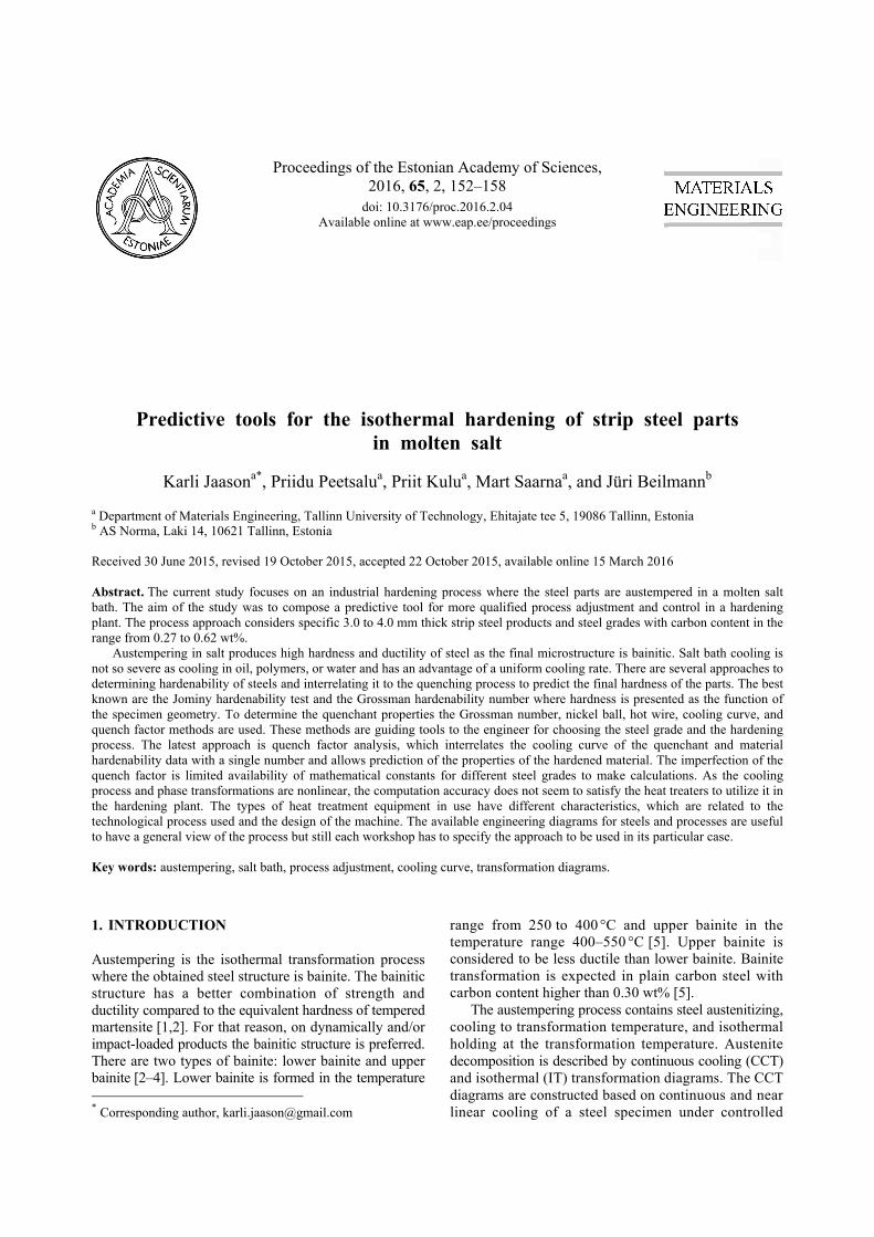
It has to be considered that the alloying elements, as well austenitizing temperature and holding time, influence the shape of the transformation diagram (Fig. 4). If the chemical composition slightly deviates from the commercial CCT diagram, Fig. 4 can be used to estimate the progress of the process.

3.4. Application of the CCT diagrams in real HT

processes

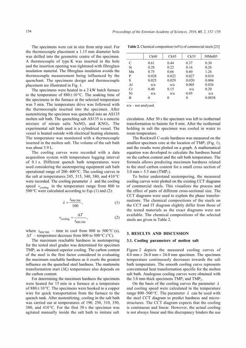
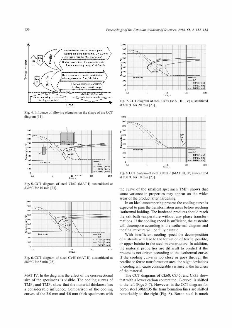
The cooling curves of the three reference specimens TMP1–3 were plotted on CCT diagrams (Figs 5–8). The CCT diagrams were chosen as reference for MAT I to


156

Fig. 4. Influence of alloying elements on the shape of the CCT diagram [11].

Fig. 5. CCT diagram of steel Ck60 (MAT I) austenitized at 830 °C for 10 min [23].

Fig. 6. CCT diagram of steel Ck45 (MAT II) austenitized at 880 °C for 5 min [23].

MAT IV. In the diagrams the effect of the cross-sectional size of the specimens is visible. The cooling curves of TMP2 and TMP3 show that the material thickness has a considerable influence. Comparison of the cooling curves of the 3.0 mm and 4.0 mm thick specimens with

Fig. 7. CCT diagram of steel Ck35 (MAT III, IV) austenitized at 880 °C for 20 min [23].

Fig. 8. CCT diagram of steel 30MnB5 (MAT III, IV) austenitized at 900 °C for 10 min [23].

the curve of the smallest specimen TMP1 shows that some variance in properties may appear on the wider areas of the product after hardening.

In an ideal austempering process the cooling curve is expected to pass the transformation areas before reaching isothermal holding. The hardened products should reach the salt bath temperature without any phase transfor-mations. If the cooling speed is sufficient, the austenite will decompose according to the isothermal diagram and the final mixture will be fully bainitic.

With insufficient cooling speed the decomposition of austenite will lead to the formation of ferrite, pearlite, or upper bainite in the steel microstructure. In addition, the material properties are difficult to predict if the process is not driven according to the isothermal curve. If the cooling curve is too close or goes through the pearlite or ferrite transformation area, the slight deviations in cooling will cause considerable variance in the hardness of the material.

The CCT diagrams of Ck60, Ck45, and Ck35 show that with a lower carbon content the ‘C-curve’ is shifted to the left (Figs 5–7). However, in the CCT diagram for boron steel 30MnB5 the transformation lines are shifted remarkably to the right (Fig. 8). Boron steel is much


157

more reliable in austempering as the process window for cooling is wider. Hence the carbon content has to be considered carefully as it directly influences the Ms-transformation temperature. For example, to obtain a bainitic microstructure with the boron steel with the carbon content of 0.30 wt% the isothermal holding above 350 °C has to be used. According to Fig. 3, the maximum hardness of 43 HRC is achieved with 0.30 wt% carbon steel at 350 °C salt bath temperature.

The process windows for deviations with Ck60 (MAT I) and Ck45 (MAT II) are narrow (Figs 5–8). It becomes even more crucial if the product’s cross-section size varies and the carbon content is lower. The steel MAT II, equal to grade Ck45 steel, should not be preferred on the products with wide cross sections. The alloying elements that affect steel hardenability should be monitored with great care, especially on the steels MAT I and MAT II.

4. CONCLUSIONS

The cooling curves were measured for the industrial austempering process in AS135 molten salt. The parameters and cooling speeds at various salt bath temperatures and for different cross sections of specimens were calculated. These parameters can be used to predict the process drive in the specific HT plant.

An equation is proposed to calculate the hardness of steels with the carbon content from 0.27 to 0.62 wt%. The equation is valid for the salt bath temperature range from 190 to 380 °C and only for small specimen cross sections of 3.0 mm 5.5 mm (TMP1). The equation was targeted for the industrial austempering process and is strongly related to the steel grades used in the study.

The CCT diagrams with plotted cooling curves from specimens with different cross sections show that MAT I (Ck60) and MAT II (Ck45) have very narrow process windows for variations in cooling. Our results suggest that MAT II should not be considered on the products thicker than 3 mm and with wide cross sections. The boron steel with a carbon content greater than 0.30 wt% is recommended for the products with thickness greater than 3.0 mm. The Ms-temperature of boron steel has to be considered carefully in austempering.

ACKNOWLEDGEMENTS

This research was supported by the European Social Fund of Doctoral Studies and the Internationalization Programme DoRa. Support by the Estonian applied research project ‘Advanced thin hard coatings in tooling’ (ESF No. 3.2.1101.12-0013) is acknowledged. The authors would like to express their gratitude to the involved company AS Norma for support and cooperation.

REFERENCES

1. Totten, G. E. Steel Heat Treatment Handbook, 2nd ed. CRC Press, Boca Raton, 2006.

2. Bhadeshia, H. K. D. H. Martensite and bainite in steels: transformation mechanism & mechanical properties. J. Phys. IV, 1997, 07(5), 367–376.

3. Abbaszadeh, K., Saghafian, H., and Kheirandish, S. Effect of bainite morphology on mechanical properties of the mixed bainite-martensite microstructure in D6AC steel. J. Mater. Sci. Technol., 2012, 28, 336–342.

4. Fuchs, A. Application of Microstructural Texture Parameters to Diffusional and Displacive Transformation Products. PhD Thesis. University of Birmingham, 2005.

5. Fielding, L. C. D. The bainite controversy. Mater. Sci. Technol., 2013, 29, 383–399.

6. Trzaska, J., Jagiełło, A., and Dobrzański, L. A. The calculation of CCT diagrams for engineering steels. Arch. Mater. Sci. Eng., 2009, 39, 13–20.

7. Wever, F. and Rose, A. Atlas zur Wärmebehandlung der Stähle. Part I. Verlag Stahleisen, Düsseldorf, 1961.

8. Atkins, M. and Met, B. Atlas of Continuous Transformation Diagrams for Engineering Steels. ASM, Ohio, 1980.

9. Smoljan, B., Smokvina Hanza, S., Tomašić, N., and Iljkić, D. Computer simulation of microstructure transformation in heat treatment processes. Journal of Achievements in Materials and Manufacturing Engineering, 2007, 24, 275–282.

10. EVS EN ISO 642. Hardenability Test by End Quenching, 1999.

11. Liedtke, D. Wärmebehandlung von Stahl - Härten, Anlassen, Vergüten, Bainitisieren. Stahl-Zentrum, Düsseldorf, 2005.

12. Kirkaldy, J. S., Thomson, B. A., and Baganis, E. A. Hardenability Concepts with Applications to Steel (Kirkaldy, J. S. and Doane, D. V., eds). AIME, Warrendale, PA, 1978, p. 82.

13. Kirkaldy, J. S. and Venugopolan, D. Phase Transformations in Ferrous Alloys (Marder, A. R. and Goldstein, J. I., eds). AIME, Warrendale, PA, 1984, p. 125.

14. Saunders, N., Guo, Z., Li, X., Midownik, A. P., and Schille, J. P. The calculation of TTT and CCT diagrams for general steels. Internal Report. Sente Software Ltd., U.K., 2004.

15. Pacheco, P. M. C. L., de Souza, L. F. G., Savi, M. A., de Oliveira, W. P., and Silva, E. D. Modeling of quenching process in steel cylinders. Mechanics of Solids in Brazil, 2007, 445–458.

16. Kobasko, N. I., Aronov, M. A., Kobessho, M., Hasegawa, M., Ichitani, K., and Dobryvechir, V. V. Critical heat flux densities and Grossmann factor as characteristics of cooling capacity of quenchants. In Recent Advances in Fluid Mechanics, Heat & Mass Transfer and Biology. WSEAS Press, 2012, 94–99.

17. Trzaska, J., Sitek, W., and Dobrzański, L. A. Selection method of steel grade with required hardenability. Journal of Achievements in Materials and Manufacturing Engineering, 2006, 17(1–2), 289–292.

18. Trzaska, J. and Dobrzański, L. A. Application of neural networks for selection of steel with the assumed hardness after cooling from the austenitising tem-perature. Journal of Achievements in Materials and Manufacturing Engineering, 2006, 16(2), 145–150.


158

19. Totten, G. E., Webster, G. M., Bates, C. E., Han, S. W., and Kang, S. H. Limitations of the use of Grossman quench severity factors. In Heat Treat: Proceedings of the 17th Heat Treating Society Conference Including the 1st International Induction Heat Treating Symposium (Milam, D., Poteet, D. A., Pfaffmann, G. D., Rudnev, V., Muehlbauer, A., and Albert, W. B., eds). ASM International, Materials Park, OH, 1998, 411–422.

20. Evancho, J. W. and Staley, J. T. Kinetics of precipitation in aluminum alloys during continuous cooling. Metall. Trans., 1974, 5, 43–47.

21. Felde, I. Report on IFHTSE liquid quenchant database project. International Heat Treatment and Surface Engineering, 2014, 8(1), 2–7.

22. Liščić, B. and Filetin, T. Measurement of quenching intensity, calculation of heat transfer coefficient and global database of liquid quenchants. Mater. Eng., 2012, 19(2), 52–63.

23. Rose, A., Peter, W., Strassburg, W., and Rademacher, L. Atlas zur Wärmebehandlung der Stähle. Part 2. Verlag Stahleisen, Düsseldorf, 1961.

Protsessi modelleerimine tööstuslikul isotermkarastamisel sulasoolavannis

Karli Jaason, Priidu Peetsalu, Priit Kulu, Mart Saarna ja Jüri Beilmann

On käsitletud erineva süsinikusisaldusega terase isotermkarastamist sulasoolavannis. Eesmärgiks on luua abivahend protsessiparameetrite täpsemaks valimiseks tööstuslikus isotermkarastusprotsessis. Käsiraamatud ja publikatsioonid pakuvad termotöötlusprotsessi seadistamiseks erinevaid lähenemisi. Sellest infost olenemata tuleb igal termotöötle-misega tegeleval ettevõttel leida protsessi usaldusväärseks seadistamiseks sobiv lähenemisviis. Töö katselises osas määrati erineva suurusega lehtmetallist katsekehade jahtumiskiirus ja terasemarkide saavutatav kõvadus erinevatel soolavanni temperatuuridel. Erinevad jahtumiskiirused saadi erineva suurusega katsekehadega, mille mõõtmed valiti lähtuvalt reaalsete toodetavate detailide ristlõigetest. Erineva süsinikusisaldusega terase margid valiti kaasatud ette-võtte karastatavaid tooteid arvestades. Antud töös leiti isotermkarastamisel kasutatava sulasoola jahtumisparameetrid (λ) ja jahtumiskiirused erinevatel soolavanni temperatuuridel. Arvutatud parameetrid on kasutatavad pidevjahtumis- (CCT) ja isotermjahtumisdiagrammidel (IT) protsessi paremaks mõtestamiseks. Töös on esitatud ka valem, mis või-maldab välja arvutada tööstuslikus isotermprotsessis saavutatava materjali kõvaduse lähtuvalt terase süsinikusisaldusest ja soolavanni temperatuurist. Tööst tuleb välja, et ettevõtte protsessis kasutatavad terasemargid C45 ja C60 on kriitilise karastatavusega, kuna detaili jahtumiskõverad on terase faasimuutuse aladele väga lähedal. Detaili ristlõike suure-nedes on ebaühtlase kõvaduse jaotuse oht üle detaili pinna, mis võib toote ekspluatatsioonis kriitiliseks osutuda. Seetõttu tuleb tähelepanelikult jälgida terase karastatust parandavate lisandite Cr, Mn ja Mo sisalduse kõikumist erinevate terasepartiide vahel. Töös on käsitletud ka boorteraseid, mille läbikarastatavus on parem kui praegu kasuta-tavatel eeleutektoidsetel madallegeerterastel. Sellest tulenevalt on otstarbekas kasutada boorterast üle 0,3% süsiniku-sisaldusega, eelkõige suuremate ristlõigete olemasolul ja üle 3 mm paksusest materjalist detailide korral. Boorteraste kasutamiseks isotermkarastusprotsessis tuleb kriitiliselt jälgida süsinikusisaldust, kuna see mõjutab kõige enam martensiidi tekke temperatuuri. Kui boorterase süsinikusisaldus on madal, saavutatakse isotermkarastamisel sitke beiniidi asemel hapra iseloomuga martensiitstruktuur.

predictive tools for the isothermal hardening of strip … tools for the isothermal hardening of...

Documents