predictive methods for end of life prognosis in composites
TRANSCRIPT

University of South CarolinaScholar Commons
Theses and Dissertations
2015
Predictive Methods for End of Life Prognosis inCompositesVamsee VadlamudiUniversity of South Carolina - Columbia
Follow this and additional works at: https://scholarcommons.sc.edu/etd
Part of the Mechanical Engineering Commons
This Open Access Thesis is brought to you by Scholar Commons. It has been accepted for inclusion in Theses and Dissertations by an authorizedadministrator of Scholar Commons. For more information, please contact [email protected].
Recommended CitationVadlamudi, V.(2015). Predictive Methods for End of Life Prognosis in Composites. (Master's thesis). Retrieved fromhttps://scholarcommons.sc.edu/etd/3145

Predictive Methods for End of Life Prognosis in Composites
by
Vamsee Vadlamudi
Bachelor of Engineering
Osmania University, 2010
Submitted in Partial Fulfillment of the Requirements
For the Degree of Master of Science in
Mechanical Engineering
College of Engineering and Computing
University of South Carolina
2015
Accepted by:
Kenneth L. Reifsnider, Director of Thesis
Prasun K. Majumdar, Reader
Lacy Ford, Vice Provost and Dean of Graduate Studies

ii
© Copyright by Vamsee Vadlamudi, 2015
All Rights Reserved.

iii
ACKNOWLEDGEMENTS
I would like to thank Dr. Kenneth Reifsnider, my research advisor, for his
invaluable advice, guidance, and support that made this work possible. His encouraging
words and positive way of thinking motivated me throughout my master’s program. It has
been enjoyable, challenging and above all an educational experience working with him.
I would also like to thank the other members of my advisory committee. I am
grateful to Dr. Majumdar for his help and support in academic activities. His enthusiasm
and dedication towards the scientific research has been an inspiration to my research.
I really appreciate the help of my colleagues, Jon-Michael Adkins, Jeffrey Baker,
Fazle Rabbi, Rassel Raihan and Faisal Haider during my research work.

iv
ABSTRACT
The long-term properties of continuous fiber reinforced composite materials are
increasingly important as applications in airplanes, cars, and other safety critical structures
are growing rapidly. The mechanical, electrical, and thermal properties of composite
materials are altered by the initiation and accumulation of discrete fracture events whose
distribution and eventual interaction defines the limits of design, such as strength and life.
There is a correlation that exists between the long term behavior of those materials under
combined mechanical, thermal, and electrical fields, and the functional properties and
characteristics of the composite materials that requires a fundamental understanding of the
material state changes caused by deformation and damage accumulation. While a strong
foundation of understanding has been established for damage initiation and accumulation
during the life of composite materials and structures, an understanding of the nature and
details that define fracture path development at the end of life has not been established.
This present research reports a multiphysics study of that progression, which is focused on
measured and predicted changes in through-thickness electric/dielectric response of
polymer based composites. Experimental data are compared to simulations of micro-defect
interactions and changes in electrical and mechanical properties. Applications of the
concepts to prognosis of behavior are discussed.

v
Also, we model a composite microstructure and analyze the material behavior using
Finite Element Analysis (FEA) and subsequently perform conformal dielectric studies on
the deformed microstructure by multiphysics simulation to relate this study to experimental
data and simulations done using the electrical analogue method. We discuss two different
models related to this, discuss results and postulate future work

vi
TABLE OF CONTENTS
ACKNOWLEDGEMENTS ................................................................................................ iii
ABSTRACT ................................................................................................................................. iv
LIST OF TABLES ............................................................................................. vii
LIST OF FIGURES .................................................................................................................. viii
CHAPTER 1 INTRODUCTION ............................................................................ 1
CHAPTER 2 LITERATURE REVIEW .................................................................................. 5
CHAPTER 3 END OF LIFE PREDICTION BY ELECTRICAL ANALOGUE
METHOD .................................................................................................................................... 10
CHAPTER 4 2D MODELING AND ANALYSIS OF COMPOSITE
MICROSTRUCTURE USING FEA ...................................................................................... 30
CHAPTER 5 DIELECTRIC STUDY OF THE COMPOSITE MICROSTRUCTURE BY
MULTIPHYSICS SIMULATION ........................................................................ 44
CHAPTER 6 THREE-PHASE MICROMECHANICS MODELING AND ANALYSIS
USING FEA ............................................................................................................................... 65
CHAPTER 7 DIELECTRIC STUDY OF THREE-PHASE MICROMECHANICS
MODEL BY MULTIPHYSICS SIMULATION .................................................................... 75
CHAPTER 8 CONCLUSION AND CONTINUING WORK .................................... 87
REFERENCES .................................................................................................. 90

vii
LIST OF TABLES
Table 3.1 Values of current at different elements in the circuit before and after shorting 13
Table 3.2: Tabulated values of current readings through elements that are a path of least
resistance. ...........................................................................................................................14
Table 3.3 Table showing variation of effective Resistance ‘R’ with No of cracks ‘N’ ...16
Table 3.4: Tabulated values of Real and Imaginary part of Impedance at different
frequencies for different stages of life ...............................................................................24
Table 3.5: Table showing variation of reactance peak frequency with % of life ............26
Table 3.6: Table showing variation of effective Resistance ‘R’ with No of cracks ‘N’....28
viii
LIST OF FIGURES
Figure 1.1 Framework created in previous work that connects material state change to
dielectric response ................................................................................................................3
Figure 1.2 Through-thickness crack pattern development (white lines) in a multiaxial
laminate subjected to fatigue loading ................................................................................. 3
Figure 1.3 Surface crack initiation (top center) in a laminate under quasi-static tensile
loading..................................................................................................................................3
Figure 2.1 Matrix crack initiation from fiber/matrix debonding ........................................ 5
Figure 2.2 Interlaminar delamination crack formed due to joining of two adjacent matrix
cracks in a fiber reinforced composite laminate ................................................................. 6
Figure 2.3 Fiber fractures in carbon-epoxy composite ........................................................7
Figure 2.4 Crack development in off-axis plies and corresponding change in secant
stiffness as a function of cyclic load cycles ........................................................................ 8
Figure 3.1 Analogue model comprising of constituent elements (Matrix and Fiber) for
simplicity............................................................................................................................10
Figure 3.2 Analogue model with highlighted fracture path and showing the presence of
damage accumulation.........................................................................................................15
Figure 3.3 Plot to show the variation of electrical compliance (Eff. Resistance ‘R’) with
No. of Cracks ‘N’ for simulated (analogue) and monotonic model ................................. 17
Figure 3.4 Expected Path of Fracture ............................................................................... 18
Figure 3.5 Predicted Fracture Path .................................................................................... 18
Figure 3.6 Anisotropic model in initial state with all of the elements intact .................... 19
Figure 3.7 Dielectric Response of the model in the initial state similar to an Insulator ....20
Figure 3.8 Model with randle’s circuit elements along fractured path ..............................21

ix
Figure 3.9 Response of the fractured model similar to a conductor ................................. 21
Figure 3.10 Observed Variation of Impedance with Frequency (left) and Nyquist Plots
(right) showing variation of impedance with life in Fazzino’s work ................................ 22
Figure 3.11 Variation of dielectric response with frequency at different stages of life .....22
Figure 3.12 Nyquist plot showing the variation of impedance with % of life ...................23
Figure 3.13 Variation of Reactance peak frequency with % of life ...................................26
Figure 3.14 Model with heterogeneous elements with fracture path highlighted ..............27
Figure 3.15 Frequency response of the heterogeneous model at Initial stage ...................27
Figure 3.16 Frequency response of the heterogeneous model at Initial stage ...................28
Figure 3.17 Plot showing variation of Effective Resistance ‘R’ and no. of cracks ‘N’ for
heterogeneous model .........................................................................................................29
Figure 4.1 Silicone Rubber matrix with steel reinforced fibers .........................................33
Figure 4.2 Plane stress quadrilateral element with four nodes ..........................................33
Figure 4.3 Final 2D Mesh of assembly generated by FEM ...............................................34
Figure 4.4 Displacement continuity between silicone rubber matrix and steel reinforced
fibers ................................................................................................................................. 34
Figure 4.5 Model with prescribed boundary conditions ....................................................35
Figure 4.6 Model showing boundary conditions and tensile loading direction ................ 36
Figure 4.7 Von Mises Stress plot on deformed contour for 25% Strain ........................... 36
Figure 4.8 Von Mises Stress plot on deformed contour for 50% Strain ............................37
Figure 4.9 Von Mises Stress plot on deformed contour for 75% Strain ............................37
Figure 4.10 Von Mises Stress plot on deformed contour for 100% Strain ....................... 38
Figure 4.11 Von Mises Stress plot on deformed contour for 125% Strain ....................... 38
Figure 4.12 Von Mises Stress plot on deformed contour for 133% Strain ....................... 39
Figure 4.13 Model showing boundary conditions and compressive loading direction .... 39

x
Figure 4.14 Von Mises Stress plot on deformed contour for 5% Strain ........................... 40
Figure 4.15 Von Mises Stress plot on deformed contour for 10% Strain ..........................40
Figure 4.16 Von Mises Stress plot on deformed contour for 15% Strain ......................... 41
Figure 4.17 Von Mises Stress plot on deformed contour for 20% Strain ......................... 41
Figure 4.18 Von Mises Stress plot on deformed contour for 25% Strain ......................... 42
Figure 4.19 Von Mises Stress plot on deformed contour for 30% Strain ......................... 42
Figure 4.20 Von Mises Stress plot on deformed contour for 35% Strain ......................... 43
Figure 5.1 Model with the top edge acting as the Terminal 1 Volt .................................. 46
Figure 5.2 Variation of Electric Field in Undeformed model ............................................47
Figure 5.3 Model under 25% tension imported for dielectric study ..................................48
Figure 5.4 Electric Field variation in model under 25% Tension ..................................... 48
Figure 5.5 Model under 50% tension imported for dielectric study ................................. 49
Figure 5.6 Electric Field variation in model under 50% Tension ..................................... 49
Figure 5.7 Model under 75% tension imported for dielectric study ................................. 50
Figure 5.8 Electric Field variation in model under 75% Tension ..................................... 50
Figure 5.9 Model under 100% tension imported for dielectric study ............................... 51
Figure 5.10 Electric Field variation in model under 100% Tension ................................. 51
Figure 5.11 Model under 125% tension imported for dielectric study ..............................52
Figure 5.12 Electric Field variation in model under 125% Tension ................................. 52
Figure 5.13 Model under 133% tension imported for dielectric study ..............................53
Figure 5.14 Electric Field variation in model under 133% Tension ................................. 53
Figure 5.15 Normalized Re (Z) vs Frequency at different stages of life .......................... 54
Figure 5.16 Change in Capacitance (∆C) vs % tensile strain ............................................55

xi
Figure 5.17 Model under 5% compression imported for dielectric study ........................ 56
Figure 5.18 Electric Field variation in model under 5% Compression............................. 56
Figure 5.19 Model under 10% compression imported for dielectric study ...................... 57
Figure 5.20 Electric Field variation in model under 10% Compression........................... 57
Figure 5.21 Model under 15% compression imported for dielectric study .......................58
Figure 5.22 Electric Field variation in model under 15% Compression............................58
Figure 5.23 Model under 20% compression imported for dielectric study .......................59
Figure 5.24 Electric Field variation in model under 20% Compression........................... 59
Figure 5.25 Model under 25% compression imported for dielectric study .......................60
Figure 5.26 Electric Field variation in model under 25% Compression............................60
Figure 5.27 Model under 30% compression imported for dielectric study .......................61
Figure 5.28 Electric Field variation in model under 30% Compression........................... 61
Figure 5.29 Model under 35% compression imported for dielectric study .......................62
Figure 5.30 Electric Field variation in model under 35% Compression........................... 62
Figure 5.31 Normalized Re (Z) vs Frequency at different stages of life under
compression .......................................................................................................................63
Figure 5.32 Change in Capacitance (∆C) vs % Compressive strain ................................. 64
Figure 6.1 Three-phase model with ring of moisture surrounding steel reinforced fiber ..66
Figure 6.2 Final mesh of three-phase model with ring of moisture surrounding steel
reinforced fibers .................................................................................................................67
Figure 6.3 Von Mises Stress plot on deformed contour for 25% Strain ............................68
Figure 6.4 Von Mises Stress plot on deformed contour for 50% Strain ........................... 68
Figure 6.5 Von Mises Stress plot on deformed contour for 75% Strain ........................... 69
Figure 6.6 Von Mises Stress plot on deformed contour for 100% Strain ......................... 69

xii
Figure 6.7 Von Mises Stress plot on deformed contour for 125% Strain ......................... 70
Figure 6.8 Von Mises Stress plot on deformed contour for 133% Strain ......................... 70
Figure 6.9 Von Mises Stress plot on deformed contour for 5% Compressive Strain ....... 71
Figure 6.10 Von Mises Stress plot on deformed contour for 10% Compressive Strain ....71
Figure 6.11 Von Mises Stress plot on deformed contour for 15% Compressive Strain ....72
Figure 6.12 Von Mises Stress plot on deformed contour for 20% Compressive Strain ....72
Figure 6.13 Von Mises Stress plot on deformed contour for 25% Compressive Strain ....73
Figure 6.14 Von Mises Stress plot on deformed contour for 30% Compressive Strain ....73
Figure 6.15 Von Mises Stress plot on deformed contour for 35% Compressive Strain ....74
Figure 7.1 Undeformed Model imported for dielectric study ............................................75
Figure 7.2 Variation of Electric Field in Undeformed model ............................................76
Figure 7.3 Variation of Electric Field in 25% tensile model ............................................ 76
Figure 7.4 Variation of Electric Field in 50% tensile model ............................................ 77
Figure 7.5 Variation of Electric Field in 75% tensile model ............................................ 77
Figure 7.6 Variation of Electric Field in 100% tensile model ...........................................78
Figure 7.7 Variation of Electric Field in 125% tensile model ...........................................78
Figure 7.8 Variation of Electric Field in 133% tensile model .......................................... 79
Figure 7.9 Variation of Normalized Impedance with % tensile strain for three-phase
model................................................................................................................................. 80
Figure 7.10 Change in capacitance ∆C vs % tensile strain for three phase-model ............80
Figure 7.11 Variation of Electric Field in 5% Compression model ..................................81
Figure 7.12 Variation of Electric Field in 10% Compression model ................................82
Figure 7.13 Variation of Electric Field in 15% Compression model ............................... 82
Figure 7.14 Variation of Electric Field in 20% Compression model ............................... 83

xiii
Figure 7.15 Variation of Electric Field in 25% Compression model ............................... 83
Figure 7.16 Variation of Electric Field in 30% Compression model ............................... 84
Figure 7.17 Variation of Electric Field in 35% Compression model ............................... 84
Figure 7.18 Variation of Normalized Impedance with % compressive strain for three phase
model..................................................................................................................................85
Figure 7.19 Change in capacitance ∆C vs % compressive strain for three phase model ..86

1
CHAPTER 1 INTRODUCTION
The long-term properties of continuous fiber reinforced composite materials are
increasingly important as applications in airplanes, cars, and other safety critical structures
are growing rapidly. Aerospace industries are more inclined to use these multifunctional
composites to reduce the weight to achieve fuel efficiency, and also for energy storage and
structural stability.
The mechanical, electrical, and thermal properties of composite materials are
altered by the initiation and accumulation of discrete fracture events whose distribution
and eventual interaction defines the limits of design, such as strength and life. Unlike
metallic materials, engineered materials (e.g. composites) are designed to develop
distributed damage consisting of various types of defects and even multiple breaks in the
same reinforcing fiber. Generally, creation of a single microscopic crack does not
individually affect the strength or life of composite materials. Therefore, the primary
interest is not in single local events but in the evolution process of multiple events that have
a collective global effect. A recent review article has emphasized the need for
understanding such nonlinearity due to damage accumulation, stating that “any analysis of
fatigue damage evolution that accounts for the irreversibility driving the damage
progression has the potential to predict fatigue life with minimum resort to empiricism.”[1]

2
In the present work, we use the calculated response of an analogue material to a
vector electric field that passes through the thickness of the composite to study defect
development, growth, coalescence, and fracture path development in a heterogeneous
material to represent material degradation (progressive damage and fracture path
development) under repeated or long-term continuous loading during the life of that
material. We simulate the dielectric response to an alternating current (AC) excitation of a
test element of the material, for the undamaged and fracture-path case, which are then
compared to laboratory experiments. As shown in Figure 1.1, for the undamaged case, for
a material such as a glass-reinforced epoxy composite, the AC response is purely capacitive
(no DC conduction), and (for linear materials, over a wide range of the response) the
absolute value of the impedance (the square root of the sum of the squares of the real and
imaginary components) is an essentially linear function of frequency with downward slope,
i.e., inversely proportional to the AC frequency (like a parallel plate capacitor). When a
fracture path has developed in the element, by definition, there will be a continuous voided
path from one physical face to the other. Let us postulate that air with some hydration or
simply diffused moisture (or other gas or fluid with some ionic content) enters that voided
space. If that diffused material is conductive, and the path is continuous, then the idealized
response (magnitude of the impedance) will not depend on the frequency of excitation (at
least to first order) as shown in Figure 1.1.
Our physical observations will focus on continuous fiber reinforced structural
composite materials, typically laminated with multiaxial ply orientations or with woven
fiber architectures, subjected to quasi-static or cyclic loading until fracture. The literature
is replete with discussions of the micro-cracking, debonding, delamination, and fiber

3
fracture events that develop during such loadings.[2-4] Examples of the damage patterns
that are observed are shown in Figures 1.2 and 1.3 which show matrix cracks and some
fiber fractures, transverse to the principal load axis, through the laminate thickness.
Figure 1.1 Framework created in previous work [1] that connects material state change to
dielectric response
Figure 1.2 Through-thickness crack pattern development (white lines) in a multiaxial
laminate subjected to fatigue loading [2-4].
Figure 1.3 Surface crack initiation (top center) in a laminate under quasi-static tensile
loading [2-4].

4
The literature says that “if a group of physical concepts or quantities are related to
each other in a certain matter, as by equations of a certain form, and another group of
concepts or quantities are interrelated in a similar manner, then an analogy may be said to
exist between the concepts of the one group and those of other group.”[5]Under combined
applied field conditions, materials degrade progressively. To evaluate such material state
changes there are many tools and methods but most of them do not give a direct and
quantitative assessment of the damage state.
Composite materials by nature are heterogeneous dielectric material systems.
When degradation happens in the material system, it develops a combination of material
state and morphology changes. Broadband Dielectric Spectroscopy (BbDS) is a robust tool
to extract the material-level information, including the morphology changes caused by
micro-detect generation and the orientation of those defects. Composite materials should
be designed in such a way that they can cope with their applied environments; to achieve
this, it is necessary to engineer the material system from the nano- and micro- scale by
controlling the shape, size, properties and interfaces of those systems. The local material
states of high performance composite structures change during their service period. In order
to achieve a prognosis of the composite durability, structural integrity, damage tolerance,
and fracture toughness, we must take into consideration the appropriate balance equations,
defect growth relationships, and constitutive equations with specified material property
variations. Local changes in the material state also have significant effects on the prognosis
of the future behavior of a composite material system.

5
CHAPTER 2 LITERATURE REVIEW
2.1 Progressive Failure in Composite Materials
Damage in composite materials under various loading conditions have been studied
and published in engineering journals since the late 1970s [6]. Various stages of
degradation from micro cracking to fiber fracture are described below
2.1.1 Microcracking
Microcracking is the basic damage mode in composite materials which initiates
changes to the material mechanical properties [7-14]. Fiber matrix debonding and initiation
of matrix microcracks is shown in Figure 2.1 [8]. After the initial development microcracks
grow through the ply thickness and width parallel to the fiber direction. Distributed
amounts of microcracks have small or no effect, rather their local stress fields typically
interact and can change the global stiffness considerably causing local stress
redistributions. Experimental data shows that changes in stiffness are not uniform
throughout the life of a material element; initially and near the onset of fracture, the change
is substantial [8-13].
Figure 2.1 Matrix crack initiation from fiber/matrix debonding. [8]

6
2.1.2 Delamination
Difference in deformation patterns in response to the local loads and stiffness
changes at local regions of composites may initiate delamination as shown in Figure 2.2.
Most delamination is initiated by microcracking [14]. This delamination can influence
changes in the laminate strength, which is not seen in the case of microcracking, and the
end result of stress redistribution associated with delamination may lead to fracture [15].
Figure 2.2 Interlaminar delamination crack formed due to joining of two adjacent matrix
cracks in a fiber reinforced composite laminate [8]
2.1.3 Fiber Fracture:
Fiber fracture is a failure mode difficult to detect and studied less completely than
any of the other damage modes in structural composites. Fiber fracture is highly coupled
to damage in fiber and matrix materials as shown in Figure 2.3 [8].

7
Figure 2.3 Fiber fractures in carbon-epoxy composite [8].
2.2 Fracture Path Development
Damage initiation in plies with different orientations occurs at different load levels
for quasi-static loading and at different rates for cyclic loading, according to well-
understood ply-level strength concepts [16]. A defining feature of this early degradation is
a decelerating damage rate; in the case of fatigue loading at a constant load level, the
microcracking of the individual plies that develop damage reaches a steady state with a
characteristic crack spacing. A sample of such behavior is shown in Figure 2.4. Matrix
cracks develop early in the plies that form cracks at the given load level, and reach a stable
number and spacing that depends on their relative stiffness in the laminate and on their
position through the thickness. The registration of those cracks along the length of the
specimen is nominally random, but in the later stages of life (or highest load levels in a
tensile test), the cracks in different plies “seek each other” to try to complete their path
through the thickness (as shown in Figure 1.2). Fiber fractures align with matrix cracks in
some cases, as is shown in the center of Figure 1.2. When this coupling creates a

8
continuous crack through the thickness, a potential “fracture plane” is formed, although it
should be remembered that since the matrix cracks run parallel to the fiber directions in
each ply, a coincident plane of cracking (through the thickness) in one position (like the
edge of the specimen shown in Figure 1.2) will not be coincident (in the same way) at some
other position across the section width.
Figure 2.4. Crack development in off-axis plies and corresponding change in secant
stiffness as a function of cyclic load cycles.
When a fracture plane forms through the thickness and across the width of the
specimen, specimen rupture occurs at the global level. That is a crack coupling process,
not represented by the data in Figure 2.4.
We know remarkably little about that end-of-life coupling process or how it forms
the fracture plane. The first question is how to measure something that is sensitive to the
damage details in that phase of the life, and how to interpret such measurements in such a
way that we can use those interpretive models to extract a “warning” of impending failure.
Fazzino et al. have suggested that dielectric response (measured through the
thickness of a laminate, and interpreted with standard dielectric spectroscopy methods) can

9
provide a multi-physics method of relating the changes in material state (reflected in
changes in AC impedance) to the micro details of damage development, and further, found
that such a method was particularly sensitive to the coupling events at the end of life [17]
and Figure 1.1. However, how the specific changes they observed were related to the details
of the coupling of microcracks and the formation of a fracture plane were not determined.
The present thesis is an attempt to contribute to that interpretation.
Various models have been established to simulate dielectric response of
heterogeneous materials such as effective medium theories, bounding methods, percolation
theory, random walks, hopping model, Fourier expansion, finite difference time domain
methods (FDTD), Monte Carlo techniques, RC network methods, and so on [18]. In the
present work we use an RC network analogue model as an approximation to a composite
material (e.g. Matrix capacitive nature modeled as capacitors, fibers as conductors or
insulators modeled as resistors).

10
CHAPTER 3 END OF LIFE PREDICTION BY ELECTRICAL ANALOGUE
METHOD 3.1 Methodology
In the present case we draw an analogy between how a fracture pattern is generated
because of a series of local stress interactions that result in a global fracture path, and local
electric current changes when resistive elements are shorted in the analogue network shown
below. We consider a Representative Volume Element (RVE) of a laminate section
(through the thickness) in which we assume that vertical elements represent constituent
material of one type (e.g., fibers) and the horizontal elements represent a second constituent
type (e.g. the matrix) as shown in Figure 3.1.
Figure 3.1 Analogue model comprising of constituent elements (Matrix and Fiber) for
Simplicity

11
For simplicity in the current discussion, we initially start with equal electrical
resistance values for fiber and matrix segments. The scope of this methodology is not
limited to constituents of the laminate; the elements in the circuit could represent different
layers of a laminate, or combinations of different materials (ex. metal and composite), or
different orientations in a laminate, etc. By varying the magnitude of the electrical
properties of the elements in the circuit we can simulate similar local mechanical or
electrical property variations.
A current equal to 1 Ampere is chosen as the power source, applied across two
opposing surface points. Distribution of that current source was selected as an analog of
how a composite material behaves locally, i.e., during loading when matrix cracking starts
and local material elements are no longer able to bear the load, the local material micro-
damage will redistribute the load to the adjacent elements. Similar behavior can be
observed in the case of a current source circuit; when we short any element (to simulate
the local failure of a matrix or fiber element), in order to maintain equilibrium the current
is redistributed in a manner that is similar to the mechanical phenomenon of local stress
redistribution in composites. It also suggests the subsequent direction of “micro-crack”
formation. We assess those indications to study the path of simulated crack growth through
the thickness of our analytical “sample”.
After shorting an element to simulate local crack formation, we re-analyze the
circuit and determine the current at each element in the circuit; we then consider the
element that has the highest subsequent difference in current to be the next micro-crack
location, which is an analogy to a local stress increase in a composite. The subsequent
crack may or may not be adjacent to the last crack location. This cycle is repeated until

12
fracture occurs i.e., to the condition where all the fractured/shorted elements create a
continuous path of least resistance through which current flows. That path simulates the
fracture path in the mechanical specimen, and changes in material state variables such as
compliance to the global applied field can be predicted and observed during the process.
3.2 Demonstration of the Method
We start with an initial random shorting of an element and then carry on,
determining how the circuit behaves as discussed above. Ideally in a “real” composite
under mechanical loading, first ply failure (or an equivalent statistical concept) can be
applied to determine which element fails first. The initial current readings of all the
elements in the present model have been tabulated under the “Before shorting” column in
Table 3.1. In this case R22 is randomly selected and initially shorted. After shorting R22,
the analysis is repeated and the current readings in all remaining elements are noted and
tabulated in the “After shorting” column in Table 3.1. Then the difference in the current at
each local ‘ammeter’ is noted and the element with the highest increase in current during
the last step is identified for shorting next. That particular element is highlighted in Table
3.1. The Value highlighted in red had the greatest increase in current, which illustrates that
the current flows through the path of least resistance, and since R22 has already been
shorted, R23 is the element that has the next highest increase in current ( R23 has been
highlighted in green in Table 3.1). This cycle of local shorting to simulate sequential
microcracking is repeated until a fracture path is formed, i.e., current passes only through
the continuous shorted path of least resistance, as shown in Table 3.2.

13
Table 3.1: Values of current at different elements in the circuit before and after shorting
Element Ammeter
Associated Value(|I| amps)
Difference
(amps)
Before
Shorting
After
Shorting
R2 TPi35 0.06818 0.05532 -0.01286
R3 TPi1 0.18182 0.17755 -0.00427
R4 TPi10 0.40909 0.40857 -0.00052
R5 TPi33 0.29545 0.28634 -0.00911
R6 TPi3 0.20454 0.19284 -0.0117
R7 TPi19 0 0.016608 0.016608
R8 TPi13 0.27272 0.26477 -0.00795
R9 TPi36 0.29545 0.30508 0.00963
R10 TPi11 0.18182 0.19197 0.01015
R11 TPi25 0.068181 0.08848 0.020299
R12 TPi14 0.20454 0.24618 0.04164
R13 TPi20 0 0.069892 0.069892
R14 TPi6 0.11363 0.11312 -0.00051
R15 TPi12 0.11363 0.11312 -0.00051
R16 TPi9 0.045454 0.034267 -0.01119
R17 TPi15 0.15909 0.14738 -0.01171
R18 TPi21 0 0.064529 0.064529
R19 TPi4 0.20454 0.18021 -0.02433
R20 TPi22 0.068181 0.047882 -0.0203
R21 TPi16 0.27272 0.21148 -0.06124
R22 TPi17 0.20454 0.3806 0.17606
R23 TPi23 0.06818 0.14159 0.073409
R24 TPi18 0.15909 0.082854 -0.07624
R25 TPi24 0.04545 0.18325 -0.02713
R26 TPi27 0.04545 0.039341 0.00611
R27 TPi26 0.15909 0.14485 -0.01424
R28 TPi28 0 0.003979 0.003979
R29 TPi29 0.15909 0.14882 -0.01027
R30 TPi34 0.04545 0.04003 -0.00542
R31 TPi31 0.11363 0.10879 -0.00484
R32 TPi32 0.11363 0.10879 -0.00484
R33 TPi38 0.11363 0.1055 -0.00813
R34 TPi37 0.11363 0.1055 -0.00813
R35 TPi39 0.18182 0.17167 -0.01015
R36 TPi40 0.40909 0.40095 -0.00814
R37 TPi41 0.18182 0.22068 0.03886
R38 TPi42 0.11363 0.10118 -0.01245
R39 TPi43 0.29545 0.27717 -0.01828
R40 TPi44 0.29545 0.32186 0.02641
R41 TPi45 0.11363 0.10118 -0.01245

14
Table 3.2: Tabulated values of current readings through elements that are a path of least
resistance.
Element Ammeter Associated Value(|I| amps)
R2 TPi35 0
R3 TPi1 0
R4 TPi10 1
R5 TPi33 0
R6 TPi3 0
R7 TPi19 0
R8 TPi13 0
R9 TPi36 0
R10 TPi11 0
R11 TPi25 1
R12 TPi14 0
R13 TPi20 0
R14 TPi6 0
R15 TPi12 0
R16 TPi9 1
R17 TPi15 1
R18 TPi21 0
R19 TPi4 0
R20 TPi22 1
R21 TPi16 0
R22 TPi17 0
R23 TPi23 1
R24 TPi18 1
R25 TPi24 1
R26 TPi27 0
R27 TPi26 0
R28 TPi28 0
R29 TPi29 0
R30 TPi34 0
R31 TPi31 0
R32 TPi32 0
R33 TPi38 0
R34 TPi37 0
R35 TPi39 1
R36 TPi40 0
R37 TPi41 0
R38 TPi42 0
R39 TPi43 1
R40 TPi44 0
R41 TPi45 0

15
The predicted fracture path is highlighted in Figure 3.2. It was observed that some
elements although shorted at some step of the path development, are not a part of the final
contiguous ‘fracture path.’ Those elements are highlighted in Figure 3.2. This is an
analogue of the physical behavior in composites in which a local failure is due to local
crack interaction and accumulation, and not due to individual crack initiation, propagation,
or growth. The staggered final fracture path in Figure 3.2 has a similar character to the
through-thickness patterns in Figure’s 1.2 and 1.3.
Figure 3.2 Analogue model with highlighted fracture path and showing the
presence of damage accumulation

16
3.3 Compliance Concepts
During the simulation analysis, after shorting of each element, the effective
resistance of the circuit is calculated and a comparison between Effective Resistance ‘R’
and No. of Cracks ‘N’ is obtained; values for one set of simulations are tabulated in Table
3.3. From the plot of such data shown in Figure 3.3, it is observed that as the
circuit/material accumulation proceeds towards failure its effective resistance reduces
(compliance increases) and at the fracture point it reaches 0 (or infinite compliance). In the
above plot the highlighted parts of the curve mark a significantly larger change in the
effective resistance of the model. This change is brought about when two local ‘cracks’
interact and a tertiary bridging crack or a “fracture plane growth” has occurred. In terms of
the physical phenomenon, this change could be attributed to fiber failure, or crack opening,
or delamination as observed in Chou’s work [19] and a similar behavior was observed in a
multiphysics model, constructed by Dr. Rassel Raihan [20].
Table 3.3 Table showing variation of effective Resistance ‘R’ with No of cracks ‘N’
No. of Cracks
‘N’
Effective Resistance ‘R’
Ohms(Homogeneous)
0 13636
1 12858
2 12430
3 11885
4 11723
5 11580
6 10299
7 7071.1
8 7049.1
9 6941.3
10 6457.5
11 5862.6
12 4792.1
13 0.01
17
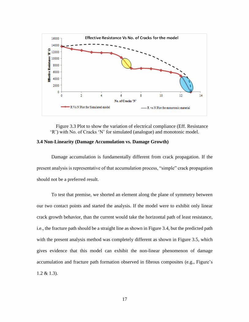
Figure 3.3 Plot to show the variation of electrical compliance (Eff. Resistance
‘R’) with No. of Cracks ‘N’ for simulated (analogue) and monotonic model.
3.4 Non-Linearity (Damage Accumulation vs. Damage Growth)
Damage accumulation is fundamentally different from crack propagation. If the
present analysis is representative of that accumulation process, “simple” crack propagation
should not be a preferred result.
To test that premise, we shorted an element along the plane of symmetry between
our two contact points and started the analysis. If the model were to exhibit only linear
crack growth behavior, than the current would take the horizontal path of least resistance,
i.e., the fracture path should be a straight line as shown in Figure 3.4, but the predicted path
with the present analysis method was completely different as shown in Figure 3.5, which
gives evidence that this model can exhibit the non-linear phenomenon of damage
accumulation and fracture path formation observed in fibrous composites (e.g., Figure’s
1.2 & 1.3).

18
Figure 3.4 Expected Path of Fracture
Figure 3.5 Predicted fracture path
3.5 Dielectric Response
3.5.1 Introduction of Anisotropy into the model
Up to this point the present model was constituted with horizontal and vertical
elements with equal initial magnitudes of resistance. In order to introduce anisotropy, a
capacitance in parallel with the resistive element is added to the horizontal elements (in
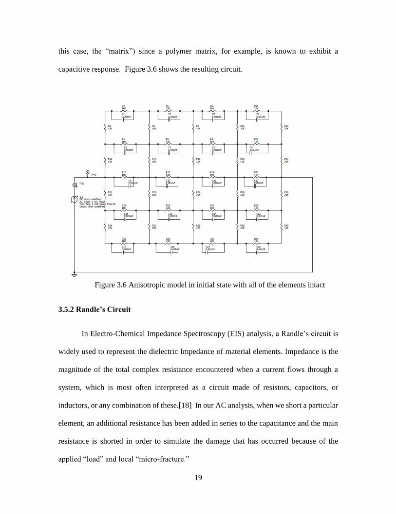
19
this case, the “matrix”) since a polymer matrix, for example, is known to exhibit a
capacitive response. Figure 3.6 shows the resulting circuit.
Figure 3.6 Anisotropic model in initial state with all of the elements intact
3.5.2 Randle’s Circuit
In Electro-Chemical Impedance Spectroscopy (EIS) analysis, a Randle’s circuit is
widely used to represent the dielectric Impedance of material elements. Impedance is the
magnitude of the total complex resistance encountered when a current flows through a
system, which is most often interpreted as a circuit made of resistors, capacitors, or
inductors, or any combination of these.[18] In our AC analysis, when we short a particular
element, an additional resistance has been added in series to the capacitance and the main
resistance is shorted in order to simulate the damage that has occurred because of the
applied “load” and local “micro-fracture.”

20
3.5.3 Initial Stage
In the initial stage under a no-load condition in the composite, i.e., without shorting
any elements as shown in Figure 3.6, the dielectric response of the anisotropic model to an
AC current was analyzed and the response was found to be equivalent to an insulator
between two plates, as shown in Figure 3.7 and observed in Figure 1.1.
Figure 3.7 Dielectric Response of the model in the initial state similar to an Insulator.
3.5.4 Final Stage
During analysis of the fracture path development, the fractured elements were
replaced by a Randle’s circuit as shown in Figure 3.8 and the dielectric response was
analyzed. It was observed that the response becomes more similar to a conductor as shown
in Figure 3.9, and observed in Figure 1.1.

21
Figure 3.8 Model with randle’s circuit elements along fractured path.
Figure 3.9 Response of the fractured model similar to a conductor.
22
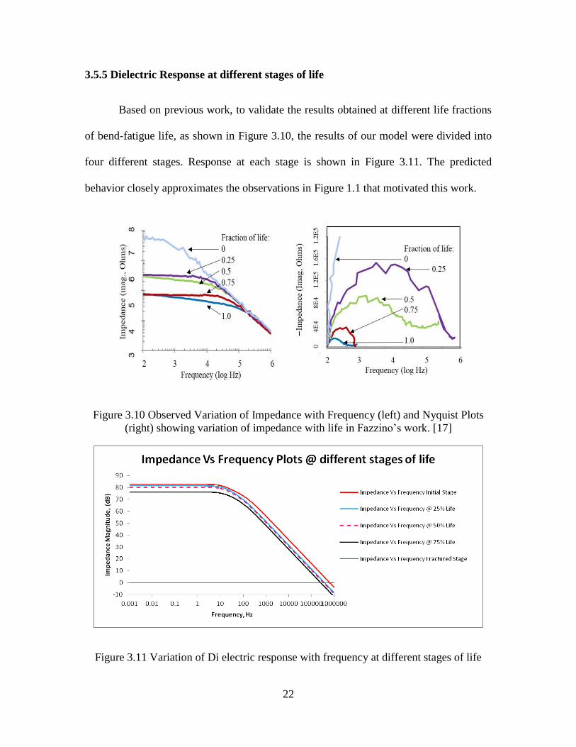
3.5.5 Dielectric Response at different stages of life
Based on previous work, to validate the results obtained at different life fractions
of bend-fatigue life, as shown in Figure 3.10, the results of our model were divided into
four different stages. Response at each stage is shown in Figure 3.11. The predicted
behavior closely approximates the observations in Figure 1.1 that motivated this work.
Figure 3.10 Observed Variation of Impedance with Frequency (left) and Nyquist Plots
(right) showing variation of impedance with life in Fazzino’s work. [17]
Figure 3.11 Variation of Di electric response with frequency at different stages of life

23
3.5.6 Nyquist Plot
By tabulating the real part of impedance, and imaginary part of impedance at
different stages of life as shown in Table 3.4 , one can create a new representation of the
change in electrical properties with increasing damage in the material. Creating a plot of
tabulated values, one can observe that as damage increases the plot shifts to the left which
indicates decreasing resistance as seen in Figure 3.12. Closely observing the plot at each
stage of life the reactance increases at low frequency values, but as the frequency increases
towards 1MHz the reactance approaches zero. These simulations are consistent with the
previous observations of Fazzino, et al.[17] We will see that changes in the shape of these
curves and the location of the intercepts are strong indicators of material state and sensitive
to the final formation of a conductive (“fracture”) path.
Figure 3.12 Nyquist plot showing the variation of impedance with % of life

24
Table 3.4: Tabulated values of Real and Imaginary part of Impedance at different frequencies for different stages of life
Frequency,
Hz
% of life
1 20 100 1E3 1E4 1E5 1E6
Re - Im Re - Im Re - Im Re - Im Re - Im Re - Im Re - Im
Initial 1.36E+4 5.86E+2 8.1E+3 5.3E+3 2.5E+3 3.7E+3 5.96E+1 6.2E+2 6.1E-1 63.65 5.9E-3 6.27 6.1E-5 0.64
25 1.19E+4 5.62E+2 6.49E+3 5.16E+3 1.27E+3 2.86E+3 2.04E+1 3.69E+2 2.12E-1 38 2.06E-3 3.76 2.12E-5 0.38
50 1.03E+4 4.74E+2 5.76E+3 4.40E+3 1.20E+3 2.57E+3 1.84E+1 3.34E+2 1.90E-1 34 1.86E-3 3.4 1.90E-5 0.34
75 6.44E+3 2.64E+2 3.99E+3 2.61E+3 9.67E+2 1.81E+3 1.59E+1 2.49E+2 1.65E-1 25.5 1.60E-3 2.55 1.65E-5 0.26
Fractured 0 0 0 0 0 0 0 0 0 0 0 0 0 0
25
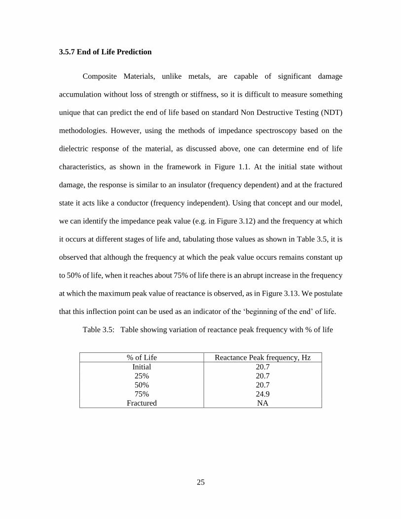
3.5.7 End of Life Prediction
Composite Materials, unlike metals, are capable of significant damage
accumulation without loss of strength or stiffness, so it is difficult to measure something
unique that can predict the end of life based on standard Non Destructive Testing (NDT)
methodologies. However, using the methods of impedance spectroscopy based on the
dielectric response of the material, as discussed above, one can determine end of life
characteristics, as shown in the framework in Figure 1.1. At the initial state without
damage, the response is similar to an insulator (frequency dependent) and at the fractured
state it acts like a conductor (frequency independent). Using that concept and our model,
we can identify the impedance peak value (e.g. in Figure 3.12) and the frequency at which
it occurs at different stages of life and, tabulating those values as shown in Table 3.5, it is
observed that although the frequency at which the peak value occurs remains constant up
to 50% of life, when it reaches about 75% of life there is an abrupt increase in the frequency
at which the maximum peak value of reactance is observed, as in Figure 3.13. We postulate
that this inflection point can be used as an indicator of the ‘beginning of the end’ of life.
Table 3.5: Table showing variation of reactance peak frequency with % of life
% of Life Reactance Peak frequency, Hz
Initial 20.7
25% 20.7
50% 20.7
75% 24.9
Fractured NA
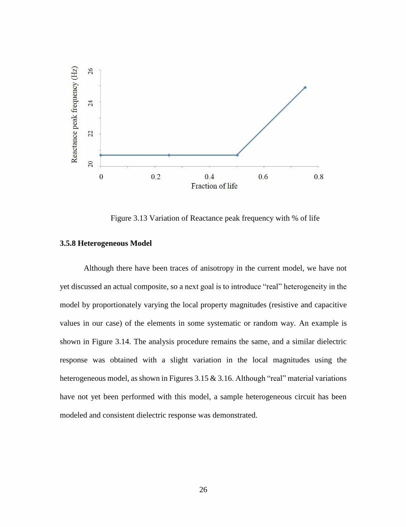
26
Figure 3.13 Variation of Reactance peak frequency with % of life
3.5.8 Heterogeneous Model
Although there have been traces of anisotropy in the current model, we have not
yet discussed an actual composite, so a next goal is to introduce “real” heterogeneity in the
model by proportionately varying the local property magnitudes (resistive and capacitive
values in our case) of the elements in some systematic or random way. An example is
shown in Figure 3.14. The analysis procedure remains the same, and a similar dielectric
response was obtained with a slight variation in the local magnitudes using the
heterogeneous model, as shown in Figures 3.15 & 3.16. Although “real” material variations
have not yet been performed with this model, a sample heterogeneous circuit has been
modeled and consistent dielectric response was demonstrated.

27
Figure 3.14 Model with heterogeneous elements with fracture path highlighted
Figure 3.15 Frequency response of the heterogeneous model at Initial stage

28
Figure 3.16 Frequency response of the heterogeneous model at Final stage
Similar to the prior anisotropic model, a plot between Effective Resistance and
Number of Cracks was created using the tabulated values shown in Table 3.6. A similar
significant change in the effective resistance was observed wherever a local interaction
created a tertiary crack or fracture, as shown in Figure 3.17.
Table 3.6: Table showing variation of effective Resistance ‘R’ with No of cracks ‘N’
No. of Cracks
‘N’
Effective Resistance ‘R’
Ohms(Heterogeneous)
0 15578
1 14883
2 14303
3 13543
4 11125
5 5607.7
6 5510.5
7 5315.8
8 4745.5
9 0

29
Figure 3.17 Plot showing variation of electrical compliance (Effective Resistance ‘R’)
and no. of cracks ‘N’ for heterogeneous model
30
CHAPTER 4 2D MODELING AND ANALYSIS OF COMPOSITE
MICROSTRUCTURE USING FEA4.1 Hyper Elastic Material
We have seen that an analogue model can predict the onset of end of life, but this
doesn’t represent a true composite material model. To simulate a ‘Real’ composite we
define a microstructure of the ‘Real’ material model and perform structural analysis using
FEA. In this process we load the structure with large strains to better understand the
material behavior under these extreme conditions. To accomplish this we chose
‘Hyperelastic’ materials that have the capability to withstand these extreme loading
conditions. Hyperelastic materials have properties of an ideal elastic material that cannot
be defined by a linear elastic material, for these materials Stress Strain relationships are
derived from Non-Linear elastic Strain Energy models such as Arruda-Boyce model,
YEOH model, Mooney-Rivlin model etc,
4.2 YEOH Model
Non-Linear elastic material models are very useful for modeling elastomers (rubber
like materials). These materials can undergo large reversible elastic deformations up to
500% strain. These materials can be characterized by stretch ratio (λ),
𝜆 = 𝐿/𝐿0

31
Where L is the deformed length and L0 is the undeformed length of the sample.
Strain energy models are based on strain invariants which are functions of the stretch ratios
in three directions, defined as
𝐼1 = 𝜆12 + 𝜆2
2 + 𝜆32
𝐼2 = 𝜆12𝜆2
2 + 𝜆22𝜆3
2 + 𝜆32𝜆1
2
𝐼3 = 𝜆12𝜆2
2𝜆32
YEOH model has proved to satisfactorily model various deformation modes
involving large strains and also has the added advantage of reduced requirements for
material testing because of its dependence only on the first strain invariant I1 [21] as defined
in the equation below.
𝑊 = ∑ 𝐶𝑖0(𝐼1 − 3)𝑖
𝑛
𝑖=1
+ ∑1
𝑑𝑘(𝐽 − 1)2𝑘
𝑛
𝑘=1
Where W is the strain energy density function, Ci0 and dk are material constants
obtained by curve fitting stress strain data, and for incompressible materials I3 = 1, J = 1
and hence strain energy density function takes the form
𝑊 = ∑ 𝐶𝑖0(𝐼1 − 3)𝑖
𝑛
𝑖=1
Silicone rubber is an elastomer that belong to this group of materials which serve
our purpose for this research
32
4.3 Material Properties of Silicone Rubber
Silicone Rubber which is one of the most commonly used hyperelastic material has
the capability to sustain larger strains up to 400%. YEOH strain energy model is used in
this simulation using a commercial FEA package (ABAQUS). To analyze Hyperelastic
materials using FEA, we need material constants of silicone rubber, which are C10 = 0.235
MPa, C20 = -0.007 MPa, C30 = 0.0008MPa, d1 = d2 = d3= 0[22]
4.4 2D Non-Linear Analysis using FEA
4. 4.1 Modeling
In the present model, we have Silicone Rubber (matrix) modeled as a sheet with
Conductors inside it uniformly spaced from each other (for simplicity). In the model
silicon rubber acts as the insulator (“matrix”) whereas steel (reinforcement) “fibers” act as
the conductors within the insulator (like a 2-D model through the thickness of a fiber
reinforced composite). Material properties of steel are E = 200 GPa, Poisson’s ratio = 0.33.
ABAQUS supports only 2D non-linear analysis for Hyperelastic materials and hence we
start with a 2D model of conductors inside an insulator as shown in Figure 4.1. The silicone
rubber sheet is 20*20 cm in size and radius of steel fiber is 1.25 cm uniformly distributed
with 4 cm from each other.

33
Figure 4.1 Silicone Rubber matrix with steel reinforced fibers
4.4.2 Meshing
The generated mesh consists of quadrilateral elements, CPS4R: A 4-node bilinear
plane stress quadrilateral, reduced integration, hourglass control as shown in Figure 4.2.
The total number of elements in the model = 2926, the total number of nodes = 3280.
CPS4R is a plane stress quadrilateral element with 4 nodes as shown in Figure 4.2. Each
node has three degrees of freedom two translation and one rotation degree of freedom.
Figure 4.2 Plane stress quadrilateral element with four nodes

34
4.4.3 Displacement Continuity
Since rubber matrix and steel fibers are two different entities we need to create a
constraint between them so that steel fibers remain connected throughout the analysis and
also to ensure that forces and displacements are transmitted from one entity to other, for
this purpose we create a displacement continuity with ‘tie’ constraint between the nodes of
these two entities as shown in Figure 4.3.
Figure 4.3 Final Mesh of the assembly with quadrilateral elements
Figure 4.4 Displacement continuity between silicone rubber matrix and steel reinforced
fibers

35
4.4.4 Boundary Conditions
The most important part of an analysis is to prescribe proper boundary conditions
for the model so that solution converges without errors. Boundary conditions for the model
are
1. Along the line passing through (0,0) and (0,20) U1 = 0, constraint in X-
direction
2. At X= 0, Y= 0 U2 = 0, constraint in Y-direction as shown in Figure 4.4
Figure 4.5 Model with prescribed boundary conditions
4.4.5 Tensile Loading
We load the model with a uniaxial displacement as shown in Figure 4.6 up
to 133% Strain (Fracture) and the Von-Mises Stress plots are shown in Figures 4.7 to
4.12

36
.
Figure 4.6 Model showing boundary conditions and tensile loading direction
Figure 4.7 Von Mises Stress plot on deformed contour for 25% Strain

37
Figure 4.8 Von Mises Stress plot on deformed contour for 50% Strain
Figure 4.9 Von Mises Stress plot on deformed contour for 75% Strain

38
Figure 4.10 Von Mises Stress plot on deformed contour for 100% Strain
Figure 4.11 Von Mises Stress plot on deformed contour for 125% Strain

39
Figure 4.12 Von Mises Stress plot on deformed contour for 133% Strain
4.4.6 Compressive Loading
For this contrasting situation, we load the model with axial displacement as shown
in Figure 4.13 up to 35% Strain (buckled) and the Von-Mises Stress plots are shown in
Figures 4.14 to 4.20.
Figure 4.13 Model showing boundary conditions and compressive loading direction
40
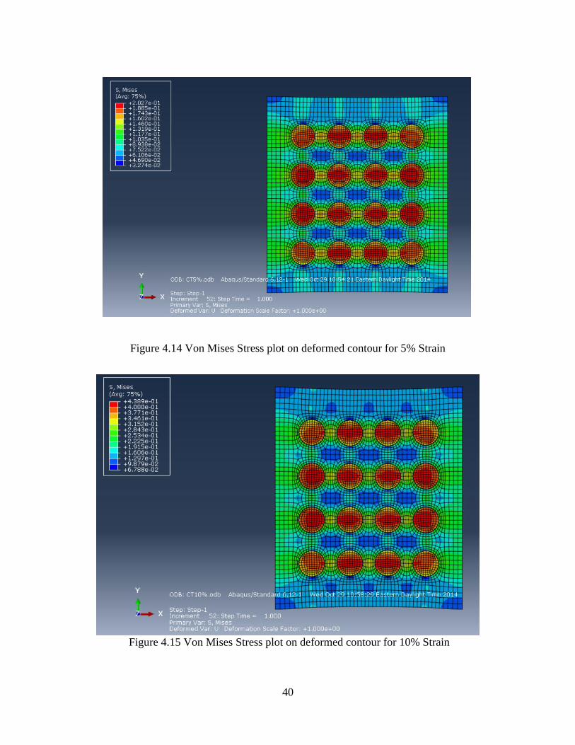
Figure 4.14 Von Mises Stress plot on deformed contour for 5% Strain
Figure 4.15 Von Mises Stress plot on deformed contour for 10% Strain

41
Figure 4.16 Von Mises Stress plot on deformed contour for 15% Strain
Figure 4.17 Von Mises Stress plot on deformed contour for 20% Strain

42
Figure 4.18 Von Mises Stress plot on deformed contour for 25% Strain
Figure 4.19 Von Mises Stress plot on deformed contour for 30% Strain

43
Figure 4.20 Von Mises Stress plot on deformed contour for 35% Strain

44
CHAPTER 5 DIELECTRIC STUDY OF THE COMPOSITE MICROSTRUCTURE BY
MULTIPHYSICS SIMULATION
5.1 Dielectric Study using Maxwell’s equations
We perform dielectric analysis of these deformed configurations using
multiphysics simulation. To help us understand the material behavior, we solve for the
Impedance and capacitance by application of Maxwell’s equations. In the dielectric study
we apply an AC signal (voltage or current) through which we can solve for Electric Field
(E) by the relation
𝐸 = −∇𝑉
The Electric field can then be subsequently related to current density J by
𝐽 = (𝜎 + 𝑗𝜔𝜀0𝜀𝑟)𝐸
Where σ is the electrical conductivity, ε0 is the permittivity of air, εr is the
permittivity or dielectric constant of the material. Current density J, helps us understand
the charge distribution throughout the configuration with the help of continuity equation
defined by
∇. (𝑑𝑠𝐽) = (𝑑𝑠𝑄)
Where ds is the shell element thickness. Charge displacement under the influence
of electric field can be studied using the relation
45
𝐷 = 𝜀0𝜀𝑟𝐸
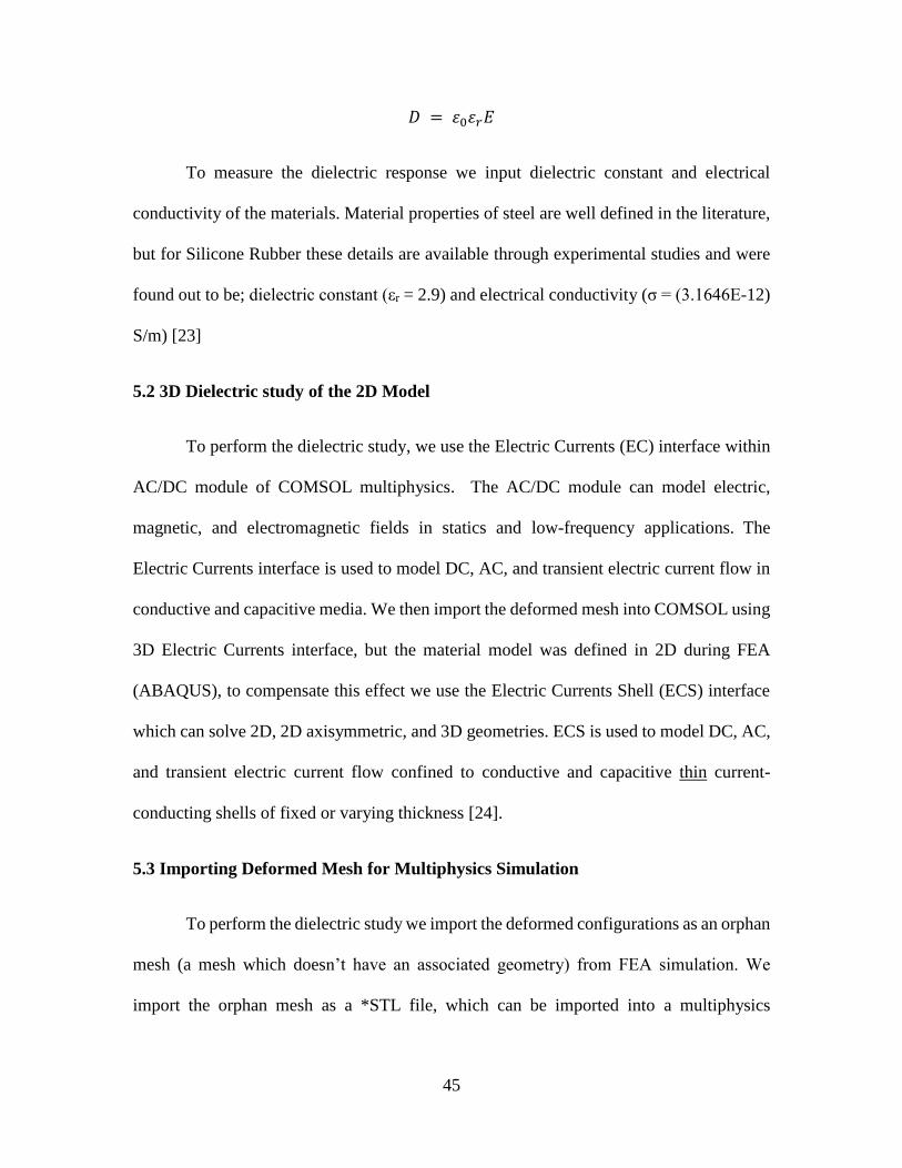
To measure the dielectric response we input dielectric constant and electrical
conductivity of the materials. Material properties of steel are well defined in the literature,
but for Silicone Rubber these details are available through experimental studies and were
found out to be; dielectric constant (εr = 2.9) and electrical conductivity (σ = (3.1646E-12)
S/m) [23]
5.2 3D Dielectric study of the 2D Model
To perform the dielectric study, we use the Electric Currents (EC) interface within
AC/DC module of COMSOL multiphysics. The AC/DC module can model electric,
magnetic, and electromagnetic fields in statics and low-frequency applications. The
Electric Currents interface is used to model DC, AC, and transient electric current flow in
conductive and capacitive media. We then import the deformed mesh into COMSOL using
3D Electric Currents interface, but the material model was defined in 2D during FEA
(ABAQUS), to compensate this effect we use the Electric Currents Shell (ECS) interface
which can solve 2D, 2D axisymmetric, and 3D geometries. ECS is used to model DC, AC,
and transient electric current flow confined to conductive and capacitive thin current-
conducting shells of fixed or varying thickness [24].
5.3 Importing Deformed Mesh for Multiphysics Simulation
To perform the dielectric study we import the deformed configurations as an orphan
mesh (a mesh which doesn’t have an associated geometry) from FEA simulation. We
import the orphan mesh as a *STL file, which can be imported into a multiphysics

46
simulation software such as COMSOL. Through the imported mesh we assign the material
properties and define boundary conditions for the analysis
5.3.1 Defining Boundary Conditions
After importing the mesh we assign material properties to entities in the model, and
define BC’s. We apply a 1 Volt AC signal across the edge perpendicular to loading
direction as shown in Figure 5.1, so the top edge would be the source with 1 Volt and
bottom would be connected to ground. Next we insulate the remaining two edges on the
sides which is represented mathematically by the equation
𝑛. 𝐽 = 0
Where n is the vector normal to the surface, also since the matrix and fibers are two
different entities, we assign a continuity boundary condition at the interface of these two
constituent elements to make sure these two entities are connected and is defined by the
equation
𝑛. (𝐽1 − 𝐽2) = 0
Figure 5.1 Model with 1 Volt signal applied perpendicular to loading direction

47
5.3.2 Dielectric study of the undeformed configuration
The undeformed configuration was imported and dielectric response was studied to
determine the variation of the Electric Fields throughout the microstructure as shown in
Figure 5.2.
Figure 5.2 Variation of Electric Field in Undeformed model
5.3.3 Dielectric study of the model loaded in Tension
In Chapter 3, we have seen that as degradation (damage) of the material increases,
we observed a variation in the dielectric response of the material. To verify this, the models
loaded in tension during FEA simulation in chapter 4 are imported and variations in the
dielectric response is studied for different mechanical load/strain cases as shown in Figures
5.3 to 5.14

48
Figure 5.3 Model under 25% tension imported for dielectric study
Figure 5.4 Electric Field variation in model under 25% Tension

49
Figure 5.5 Model under 50% tension imported for dielectric study
Figure 5.6 Electric Field variation in model under 50% Tension
50
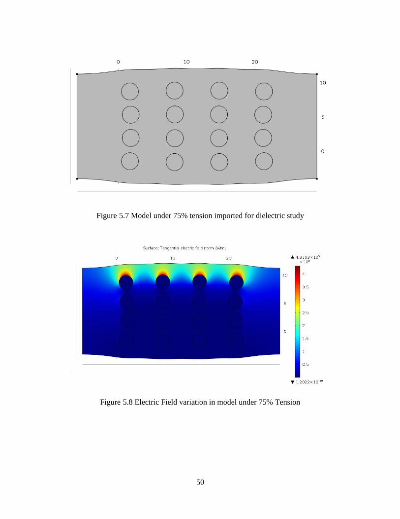
Figure 5.7 Model under 75% tension imported for dielectric study
Figure 5.8 Electric Field variation in model under 75% Tension

51
Figure 5.9 Model under 100% tension imported for dielectric study
Figure 5.10 Electric Field variation in model under 100% Tension

52
Figure 5.11 Model under 125% tension imported for dielectric study
Figure 5.12 Electric Field variation in model under 125% Tension

53
Figure 5.13 Model under 133% tension imported for dielectric study
Figure 5.14 Electric Field variation in model under 133% Tension
5.3.4 Comparison of Dielectric response at various Tensile loads
As damage in the material increases, we observed a substantial variation in the
dielectric response of the material in chapter 3, we observe a similar variation in the
response during this multiphysics simulation. We see a net decrease of 60% in Normalized
Impedance, Re (Z) of the model as shown in Figure 5.15. Normalized impedance in the
model is calculated as
54
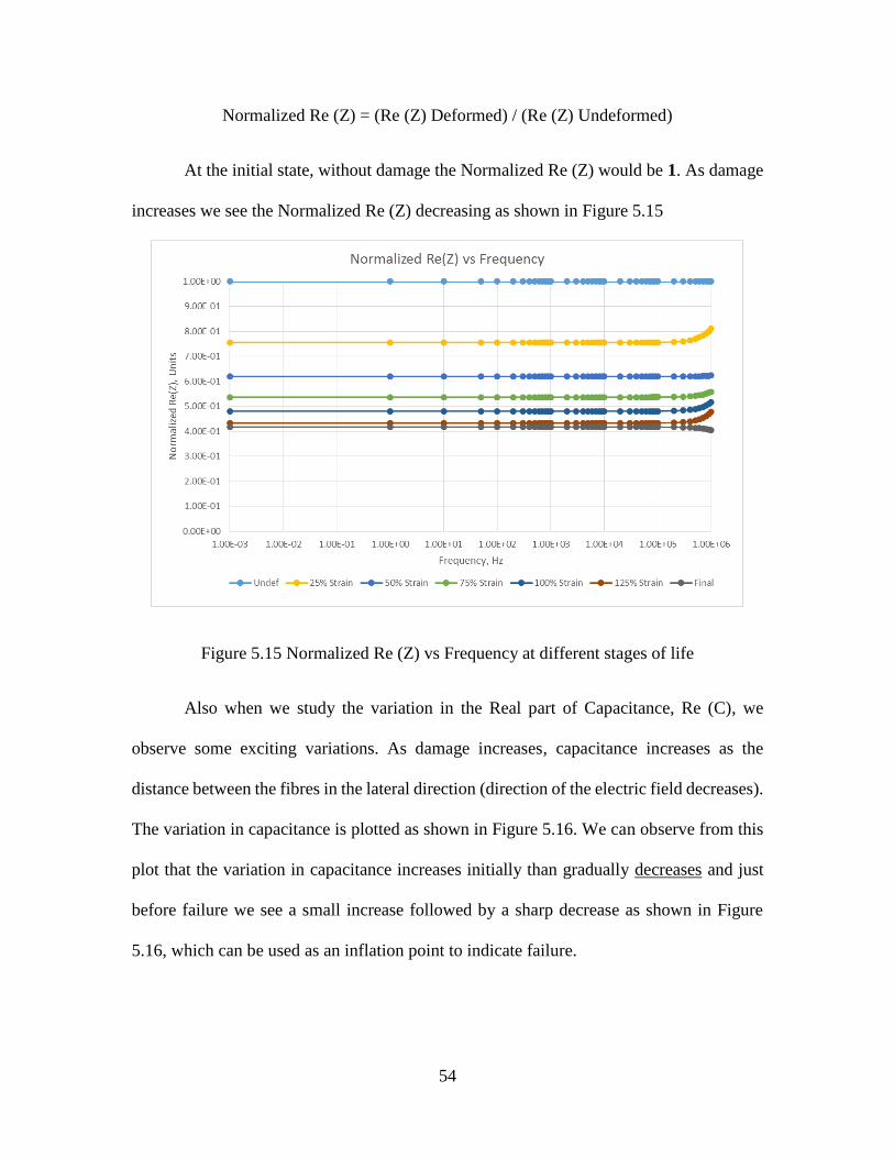
Normalized Re (Z) = (Re (Z) Deformed) / (Re (Z) Undeformed)
At the initial state, without damage the Normalized Re (Z) would be 1. As damage
increases we see the Normalized Re (Z) decreasing as shown in Figure 5.15
Figure 5.15 Normalized Re (Z) vs Frequency at different stages of life
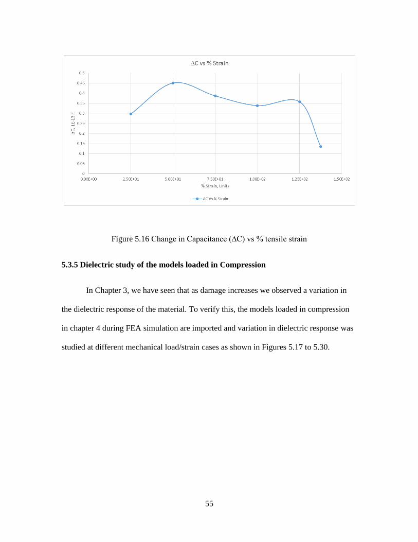
Also when we study the variation in the Real part of Capacitance, Re (C), we
observe some exciting variations. As damage increases, capacitance increases as the
distance between the fibres in the lateral direction (direction of the electric field decreases).
The variation in capacitance is plotted as shown in Figure 5.16. We can observe from this
plot that the variation in capacitance increases initially than gradually decreases and just
before failure we see a small increase followed by a sharp decrease as shown in Figure
5.16, which can be used as an inflation point to indicate failure.
55
Figure 5.16 Change in Capacitance (∆C) vs % tensile strain
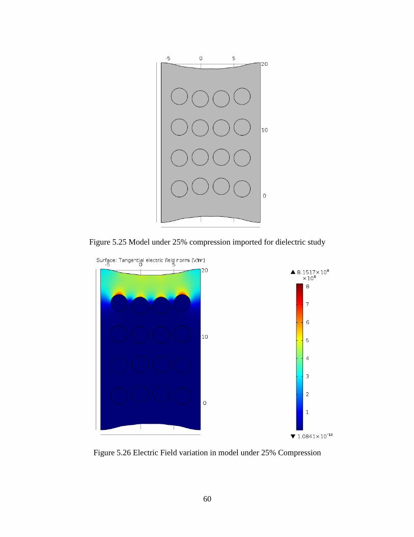
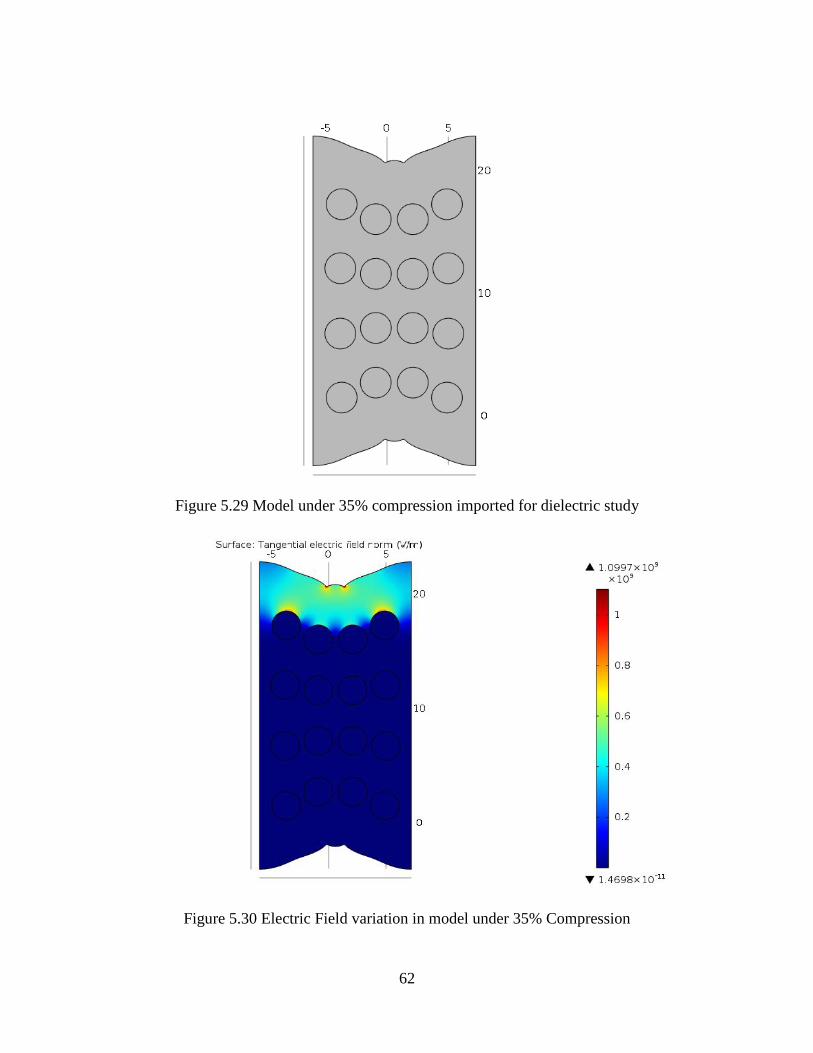
5.3.5 Dielectric study of the models loaded in Compression
In Chapter 3, we have seen that as damage increases we observed a variation in
the dielectric response of the material. To verify this, the models loaded in compression
in chapter 4 during FEA simulation are imported and variation in dielectric response was
studied at different mechanical load/strain cases as shown in Figures 5.17 to 5.30.

56
Figure 5.17 Model under 5% compression imported for dielectric study
Figure 5.18 Electric Field variation in model under 5% Compression

57
Figure 5.19 Model under 10% compression imported for dielectric study
Figure 5.20 Electric Field variation in model under 10% Compression

58
Figure 5.21 Model under 15% compression imported for dielectric study
Figure 5.22 Electric Field variation in model under 15% Compression

59
Figure 5.23 Model under 20% compression imported for dielectric study
Figure 5.24 Electric Field variation in model under 20% Compression
60
Figure 5.25 Model under 25% compression imported for dielectric study
Figure 5.26 Electric Field variation in model under 25% Compression

61
Figure 5.27 Model under 30% compression imported for dielectric study
Figure 5.28 Electric Field variation in model under 30% Compression
62
Figure 5.29 Model under 35% compression imported for dielectric study
Figure 5.30 Electric Field variation in model under 35% Compression

63
5.3.6 Comparison of Dielectric study at various Compression loads
As damage in the material increases, we observed that impedance decreases during
tensile loading, but in case of compression we observe that Impedance increases. We
observed a net increase of 73% in Normalized Impedance, Re (Z) of the model as shown
in Figure 5.31.
At the initial state, without damage the Normalized Re (Z) would be 1. As damage
increases we see the Normalized Re (Z) decreasing as shown in Figure 5.31.
Figure 5.31 Normalized Re (Z) vs Frequency at different stages of life under compression

64
Also when we study the variation in Real part of Capacitance, Re (C) we observe a
steady plot. As damage increases Capacitance decreases as the distance between the fibres
in the lateral direction (direction of electric field increases). The variation in capacitance is
plotted as shown in Figure 5.32. We can observe from this plot variation in capacitance
decreases steadily.
Figure 5.32 Change in Capacitance (∆C) vs % Compressive strain

65
CHAPTER 6 THREE-PHASE MICROMECHANICS MODELING AND ANALYSIS
USING FEA
6.1 Introducing third phase in to the model
In the above chapters we have noticed a variation in dielectric response as damage
increases in the material. In real-time conditions, as material degrades we see moisture or
other impurities settling in these cracks that can influence the response and performance of
the material. In order to simulate this effect we introduced a third phase which represents
moisture in this model.
6.2 Material Properties of the third phase
To analyze the three-phase model using FEA, we define moisture as a linear elastic
material with Poisson’s ratio ν = 0.5, since moisture (water) can be assumed as a liquid,
where forces act equally in all directions. Taking ν = 0.5 would lead to singularity in the
computation so we approximate it to 0.48. For an elastic material we need to define
Young’s Modulus (E) of the material. For moisture, we derive this value from the relation
𝑬 = 𝟑 × 𝑲 × (𝟏 − 𝟐𝝂)
Where E is the Young’s Modulus, K is the Bulk modulus and ν is the poisson’s
ratio. For moisture (water) K= 2.2E9 Pa, Hence from the relation we get E = 2.64E8 Pa.

66
6.3 2D nonlinear analysis of the three-phase model
6.3.1 Modeling Moisture as third phase
To model third phase, we create a ring of 1.25 cm radius around 1.23 cm fiber as
shown in Figure 6.1. Then we assemble the model, mesh and assign displacement
continuity as done in chapter 4. The final mesh assembly is shown in Figure 6.2.
Figure 6.1 Three-phase model with ring of moisture surrounding steel reinforced fiber
The mesh consists of quadrilateral elements, CPS4R: A 4-node bilinear plane stress
quadrilateral, reduced integration, hourglass control as shown in Figure 6.2. The total
number of elements in the model = 5088, the total number of nodes = 6209.

67
Figure 6.2 Final mesh of three-phase model with ring of moisture surrounding steel
reinforced fibers
6.3.2 Model loaded in Tension
The Boundary conditions for the three-phase model remains the same as discussed
in chapter 4. We deform the model by uni-axial displacement up to 133% Strain (Fracture)
and the Von-Mises Stress plots are shown in Figures 6.3 to 6.8. It is observed that
deformation patterns almost remain the same even with the inclusion of third phase

68
Figure 6.3 Von Mises Stress plot on deformed contour for 25% Strain
Figure 6.4 Von Mises Stress plot on deformed contour for 50% Strain

69
Figure 6.5 Von Mises Stress plot on deformed contour for 75% Strain
Figure 6.6 Von Mises Stress plot on deformed contour for 100% Strain

70
Figure 6.7 Von Mises Stress plot on deformed contour for 125% Strain
Figure 6.8 Von Mises Stress plot on deformed contour for 133% Strain

71
6.3.3 Model loaded in Compression
We deform the model by uni-axial displacement up to 35% Strain (buckling) and
the Von-Mises Stress plots are shown in Figures 6.9 to 6.15. It is observed that deformation
patterns almost remain the same even with the inclusion of third phase.
Figure 6.9 Von Mises Stress plot on deformed contour for 5% Compressive Strain
Figure 6.10 Von Mises Stress plot on deformed contour for 10% Compressive Strain

72
Figure 6.11 Von Mises Stress plot on deformed contour for 15% Compressive Strain
Figure 6.12 Von Mises Stress plot on deformed contour for 20% Compressive Strain

73
Figure 6.13 Von Mises Stress plot on deformed contour for 25% Compressive Strain
Figure 6.14 Von Mises Stress plot on deformed contour for 30% Compressive Strain

74
Figure 6.15 Von Mises Stress plot on deformed contour for 35% Compressive Strain

75
CHAPTER 7 DIELECTRIC STUDY OF THREE-PHASE MICROMECHANICS
MODEL BY MULTIPHYSICS SIMULATION
7.1 Dielectric study of three-phase Micromechanics model loaded in tension
After importing the deformed mesh we assign material properties to entities in the
model and define BC’s. For the third phase, moisture dielectric constant (ε) = 1 and
electrical conductivity (σ) = 5E-4 S/m. Undeformed model is imported as shown in Figure
7.1 to understand variation of Electric Field throughout the model as shown in Figures 7.2
to 7.8.
Figure 7.1 Undeformed Model imported for dielectric study

76
Figure 7.2 Variation of Electric Field in Undeformed model
Figure 7.3 Variation of Electric Field in 25% tensile model

77
Figure 7.4 Variation of Electric Field in 50% tensile model
Figure 7.5 Variation of Electric Field in 75% tensile model

78
Figure 7.6 Variation of Electric Field in 100% tensile model
Figure 7.7 Variation of Electric Field in 125% tensile model

79
Figure 7.8 Variation of Electric Field in 133% tensile model
7.2 Comparison of Dielectric response at various Tensile loads
As damage in the material increases, we observed a change in the dielectric
response of the material in chapter 5, and we observe a similar change in the response for
this three-phase model. We see a net decrease of 60% in Normalized Impedance, Re (Z) of
the model as shown in Figure 7.9.
At Initial state, without damage the Normalized Re (Z) would be 1. As damage
increases we see the Normalized Re (Z) decreasing as shown in Figure 7.9

80
Figure 7.9 Variation of Normalized Impedance with % tensile strain for three-phase
model
Also when we study the variation in Real part of Capacitance, Re (C) we observe
similar variation as seen in two-phase model. As damage increases Capacitance increases
as the distance between the fibres in the direction of electric field decreases. The variation
in capacitance with damage is plotted as shown in Figure 7.10.
Figure 7.10 Change in capacitance ∆C vs % tensile strain for three-phase model
81
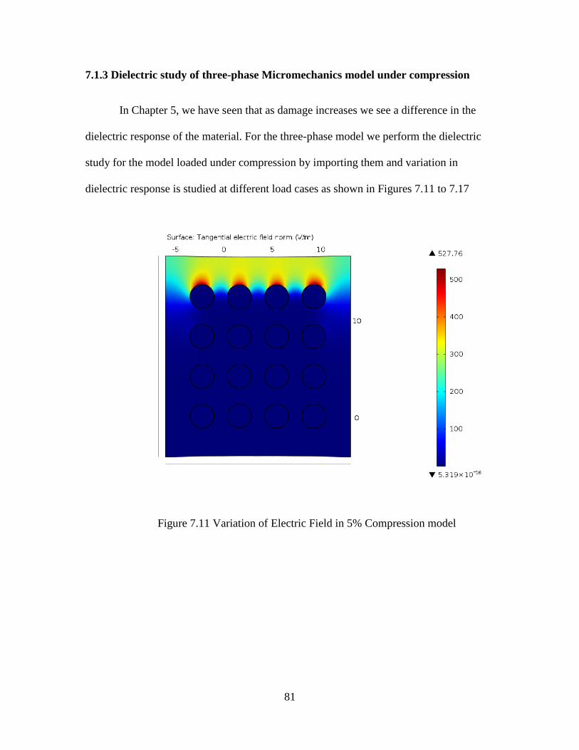
7.1.3 Dielectric study of three-phase Micromechanics model under compression
In Chapter 5, we have seen that as damage increases we see a difference in the
dielectric response of the material. For the three-phase model we perform the dielectric
study for the model loaded under compression by importing them and variation in
dielectric response is studied at different load cases as shown in Figures 7.11 to 7.17
Figure 7.11 Variation of Electric Field in 5% Compression model

82
Figure 7.12 Variation of Electric Field in 10% Compression model
Figure 7.13 Variation of Electric Field in 15% Compression model

83
Figure 7.14 Variation of Electric Field in 20% Compression model
Figure 7.15 Variation of Electric Field in 25% Compression model
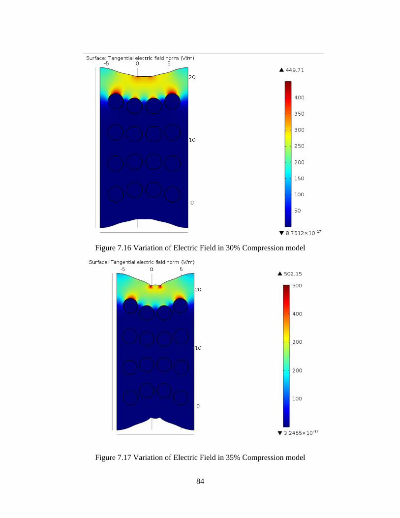
84
Figure 7.16 Variation of Electric Field in 30% Compression model
Figure 7.17 Variation of Electric Field in 35% Compression model

85
7.1.4 Comparison of Dielectric response at various compressive loads
As damage in the material increases, we observed a change in the dielectric
response of the material in chapter 5, we observe a similar change in the response in this
three-phase model. We see a net increase of 73% in Normalized Impedance, Re (Z) of the
model as shown in Figure 7.18.
At the initial state, without damage the Normalized Re (Z) would be 1. As damage
increases we see the Normalized Re (Z) decreasing as shown in Figure 7.18
Figure 7.18 Variation of Normalized Impedance with % compressive strain for three
phase model

86
Also when we study the variation in Real part of Capacitance, Re (C) we observe
similar variation as seen in two phase model. As damage increases Capacitance decreases
as the distance between the fibres in the direction of electric field increases. The variation
in capacitance is plotted as shown in Figure 7.19.
Figure 7.19 Change in capacitance ∆C vs % compressive strain for three phase model

87
CHAPTER 8 CONCLUSION AND CONTINUING WORK
We have shown that an alternating current analogue simulation of microcrack
interaction and through-thickness fracture path development correctly predicts many of the
features of the broadband dielectric spectroscopy (BBDS) measured response of
continuous fiber composites loaded to failure in quasi-static and fatigue conditions. This
multiphysics approach provides useful new insights into the nature of through-thickness
damage and fracture plane development, while providing physical associations that are part
of a foundation for the interpretation of broadband dielectric spectroscopy data for
subsequent predictive theories.
We have also observed that the global compliance to applied AC electrical fields is
closely related to the material compliance to mechanical stress fields during fracture path
development. A key feature of that response was the observation of abrupt changes in
multiphysics compliance (mechanical and electrical) that were identified with the onset of
discrete fracture path instability and rupture. We also identified an inflection point in the
frequency dependence of AC impedance that was an indicator of the ‘beginning of the end
of life.’
We have provided only a few first steps in simulating the multiphysics response
associated with the development of discrete fracture paths in fibrous composites; much is
yet to be done. However, on the basis of the present work, it would appear that the dielectric
response through the thickness of continuous fiber reinforced composite materials seems

88
to be uniquely sensitive to the details of microdamage accumulation and especially to “end
of life” events such as the formation of contiguous incipient fracture paths, local micro-
buckling and highly nonlinear deformation associated with shape change.
We have modeled composite specimens loaded with various tensile and
compressive loads and observed various failure patterns, and studied dielectric response of
the materials under those conditions. We have shown that in the two phase model, when
loaded in tension we see a 60% decrease in the impedance and found some excitement in
the change in capacitance, which if properly studied could be used to identify an inflection
point that predicts onset of failure. When loaded in compression we have shown a 73%
increase in impedance but the change in capacitance was rather in a steady rate. However
in the three-phase micromechanics model we didn’t observe much difference from the two
phase model, which is logical as the ring of moisture surrounding the conductor is not
significant enough to effect the results in the simulation.
Next we wish to perform two phase and three-phase micromechanics model studies
of a matrix material having higher conductivity than the fiber, which could respond
differently under these loads and see if we could find variation in the dielectric response.
As of now we have studied dielectric response with a field acting perpendicular to the
loading direction, we also wish to perform the study with a field parallel to the loading
direction to help us understand the material behavior under these variations.
However, the current study has clearly established that the dielectric response of a
material through the thickness of a heterogeneous material is substantially and distinctly
related to the development of deformations and defect development that are to be expected

89
during the development of a fracture path. This is a step in the direction of understanding
this essential but neglected element of the “end of life” events in fibrous composite
materials.

90
REFERENCES
[1]. Majumdar P., Reifsnider K, “Study of Fracture Path Development and Remaining
Life Utilizing Low-Frequency Electrical Response,” Grant #NNX13AD43A-USC.
[2]. Gudmumdson P., and Zhang, W., Thermoelastic properties of microcracked
composite laminates, Mechanics of Composite Materials, 29 #2, (1993) 107-114.
[3]. Damage in Composite Materials, ASTM STP 775, K. L. Reifsnider, Ed., American
Society for Testing and Materials (1982) DOI: 10.1520/STP775-EB
[4]. Jamison, R.D., Schulte, K., Reifsnider, K., Stinchcomb, W., Characterization and
Analysis of Damage Mechanisms in Tension-Tension Fatigue of Graphite/Epoxy
Laminates, in Effects of Defects in Composite Materials, ASTM STP 836, ASTM
(1984) 21-55
[5]. F.A.Firestone, A New analogy between Mechanical and Electrical Systems,
Journal of the Acoustical Society , (Jan 1933) 250-267
[6]. Qian, H., Kucernak, A. R., Greenhalgh, E. S., Bismarck, A., & Shaffer, M. S..
Multifunctional structural supercapacitor composites based on carbon aerogel
modified high performance carbon fiber fabric. ACS applied materials &
interfaces, 5(13), 6113-6122 (2013).
[7]. Reifsnider, K. L.; Ed. Damage in Composite Materials. ASTM 775, American
Society for Testing and Materials, Philadelphia 1982

91
[8]. Reifsnider, K.L., and Case, S. W., Damage Tolerance and Durability of Material
Systems. New York: John Wiley and Sons (2002).
[9]. Highsmith, A. L., & Reifsnider, K. L. Stiffness-reduction mechanisms in
composite laminates. Damage in composite materials, ASTM STP, 775, 103-
117(1982).
[10]. Nairn, J. A. Matrix microcracking in composites. Polymer matrix composites, 2,
403-432 (2000).
[11]. Talreja, R. Transverse cracking and stiffness reduction in composite
laminates. Journal of composite materials, 19(4), 355-375 (1985).
[12]. Talreja, R., & Singh, C. V. Damage and failure of composite materials.
Cambridge University Press (2012).
[13]. Varna, J., & Krasnikovs, A. Transverse cracks in cross-ply laminates 2. Stiffness
degradation. Mechanics of composite materials, 34(2), 153-170 (1998).
[14]. O'brien, T. K. Characterization of delamination onset and growth in a composite
laminate. Damage in composite materials, ASTM STP, 775(2), 140-167 (1982).
[15]. Stinchcomb, W. W., & Bakis, C. E. Fatigue behavior of composite
laminates. Fatigue of composite materials, 4, 105-180 (1990).
[16]. Reifsnider, K., and Case, S.W., Durability and Damage Tolerance of Material
Systems, John Wiley & Sons (2002)
[17]. Fazzino, P., Reifsnider, K., Majumdar, P., “Impedance spectroscopy for
progressive damage analysis in woven composites,” Composites Science and
Technology 169 (2009) 2008-2014
92
[18]. Huang, M, Yang, J, Xiao, Z., Sun, J., and Peng, J., “Modeling the Dielectric
Response in Heterogeneous Materials using 3D RC Networks,” Modern Physics
Letters B, 23, No. 25 (2009) 3023–3033
[19]. Chou, T-W., “Multifunctional Carbon Nanotube–Based Sensors for Damage
Detection and Self Healing in Structural Composites,” contractors report, Grant
No: FA9550-09-1-0218 (2009)
[20]. Reifsnider, K., Raihan, R. and Liu, Q., “Rational Durability Design of
Heterogeneous Functional Materials: Some First Principles,” Mechanics of
Composite Materials, 49#1 (2013) 31-54
[21]. A Comparative Study of Several Material Models for Prediction of Hyperelastic
Properties: Application to Silicone-Rubber and Soft Tissues, P. A. L. S. Martins,
R. M. Natal Jorge and A. J. M. Ferreira, Strain (2006) 42, 135–147
[22]. The Yeoh model applied to the modeling of large deformation contact/impact
problems Christine Renaud, Jean-Michel Cros, Zhi-Qiang Feng, Bintang Yang,
International Journal of Impact Engineering 36 (2009) 659–666
[23]. Electrical properties of Silicone Rubber Retrieved from:
http://www.azom.com/properties.aspx?ArticleID=920
[24]. COMSOL Multiphysics© Reference Guide, Version 4.3a (2012).