Submitted 10 March 2014Accepted 28 May 2014Published 17 June 2014

Corresponding authorSimon van Mourik,simon.vanmourik@wur.nl

Academic editorClaus Wilke

Additional Information andDeclarations can be found onpage 13

DOI 10.7717/peerj.433

Copyright2014 van Mourik et al.

Distributed underCreative Commons CC-BY 4.0

OPEN ACCESS

Prediction uncertainty assessment of asystems biology model requires a sampleof the full probability distribution of itsparametersSimon van Mourik1,2, Cajo ter Braak1, Hans Stigter1 andJaap Molenaar1,2

1 Biometris, Wageningen University and Research Center, Wageningen, The Netherlands2 Netherlands Consortium for Systems Biology, Amsterdam, The Netherlands

ABSTRACTMulti-parameter models in systems biology are typically ‘sloppy’: some parame-ters or combinations of parameters may be hard to estimate from data, whereasothers are not. One might expect that parameter uncertainty automatically leadsto uncertain predictions, but this is not the case. We illustrate this by showing thatthe prediction uncertainty of each of six sloppy models varies enormously amongdifferent predictions. Statistical approximations of parameter uncertainty may leadto dramatic errors in prediction uncertainty estimation. We argue that predictionuncertainty assessment must therefore be performed on a per-prediction basis usinga full computational uncertainty analysis. In practice this is feasible by providing amodel with a sample or ensemble representing the distribution of its parameters.Within a Bayesian framework, such a sample may be generated by a Markov ChainMonte Carlo (MCMC) algorithm that infers the parameter distribution based onexperimental data. Matlab code for generating the sample (with the DifferentialEvolution Markov Chain sampler) and the subsequent uncertainty analysis usingsuch a sample, is supplied as Supplemental Information.

Subjects Bioinformatics, Computational Biology, Mathematical Biology, StatisticsKeywords Parameter uncertainty, Prediction uncertainty, Bayesian statistics, MCMC

INTRODUCTIONBy combining experiments and mathematical model analysis, systems biology tries to

unravel the key mechanisms behind biological phenomena. This has led to a steadily

growing number of experiment-driven modeling techniques (Klipp et al., 2008; Stumpf,

Balding & Girolami, 2011). Useful models provide insight and falsifiable predictions and

the dynamic models used in systems biology are no exception. A complicating factor

in multi-parameter models is that often many parameters are largely unknown. Even

among similar processes parameter values may vary multiple orders of magnitude, and

experimentally they are often hard to infer accurately (Maerkl & Quake, 2007; Buchler &

Louis, 2008; Teusink et al., 2000).

How to cite this article van Mourik et al. (2014), Prediction uncertainty assessment of a systems biology model requires a sample of thefull probability distribution of its parameters. PeerJ 2:e433; DOI 10.7717/peerj.433

A standard procedure for parameter estimation is via a collective fit, i.e., estimating

the values of the unknown parameters simultaneously by fitting the model to time series

data, resulting in a calibrated model. This approach has to cope with several obstacles,

such as measurement errors, biological variation, and limited amounts of data. Another

often met problem is that different parameters may have correlated effects on the measured

dynamics leading to highly uncertain or even unidentifiable parameter estimates (Zak et

al., 2003a; Zak et al., 2003b; Raue et al., 2009). Systems biology models are typically ‘sloppy’

in that some parameters or combinations of parameters are well defined, whereas many

others are not (Brown & Sethna, 2003; Gutenkunst et al., 2007b). It was argued on the basis

of this sloppiness that collective fits are more promising for obtaining useful predictions

than direct parameter measurements, and that “modelers should focus on predictions

rather than on parameters” (Gutenkunst et al., 2007b). One might expect that sloppiness

and the associated parameter uncertainty automatically lead to uncertain predictions, but

that is not necessarily so. For example, in the literature a model has been reported with 48

parameters calibrated to only 68 data points and with highly uncertain parameter values,

but the predictions were quite accurate (Brown et al., 2004).

In this paper we fit an illustrative model and a diverse set of six systems biology

models from the BioModels database (Li et al., 2010) to different amounts of (simulated)

time series data. For each model, we study the prediction uncertainty of a number of

predictions by a full computational uncertainty analysis. We measure the uncertainty in the

predicted time course by the dimensionless quantifier Q0.95 which has the nice property

that Q0.95 < 1 indicates tight predictions, whereas Q0.95 ≥ 1 implies uncertainty in the

dynamics that is likely to obscure biological interpretation. Using this quantifier, we show

that some models allow more accurate predictions than others, but, more importantly,

that the uncertainty of the predictions may greatly vary within one model. We argue that

prediction uncertainty assessment must therefore be performed on a per-prediction basis

using a full computational uncertainty analysis (Savage, 2012). We indicate how such an

analysis can be performed in a relatively easy way. It requires a sample representing (strictly

speaking, approximating) the distribution of the parameters of the model. The importance

of such a sample (an ensemble of parameter sets) for uncertainty analysis has been pointed

out earlier (Brown & Sethna, 2003; Gutenkunst et al., 2007a), but we go one step further and

recommend modellers to make available not only the mathematical model and its typical

parameter values and operating conditions, but also a sample representing the distribution

of its parameters (Fig. 1). For other reasons, such as verification and reproducibility of the

research, data and software to obtain such a sample should also be made available.

Within the Bayesian framework (Jaynes, 2003; MacKay, 2003) this is a sample as

generated by an MCMC algorithm (Robert, Marin & Rousseau, 2011) that collectively

fits the parameters of the model to experimental data. We advocate the Bayesian framework

as it allows inclusion of prior information (based on prior parameter knowledge, general

biological considerations (Grandison & Morris, 2008) and direct parameter measurements)

to be combined with the information contained in time series data. If no prior information

van Mourik et al. (2014), PeerJ, DOI 10.7717/peerj.433 2/17

Figure 1 Flowchart of parameter estimation and uncertainty analysis. The model dynamics are fittedto noisy time series data, typically by an MCMC algorithm, resulting in a sample of parameter valuesrepresenting their posterior distribution. Typical applications of this distribution are the computationof a credible region of parameters (showing parameter uncertainty) and full computational uncertaintyanalysis of predictions.

is available, a noninformative prior can be constructed. For a discussion on prior selection,

see Robert, Marin & Rousseau (2011).

It is useful at this point to compare the Bayesian approach with the frequentist approach

of prediction profile likelihood (PPL) (Kreutz et al., 2013) which is another approach

to uncertainty analysis. PPL requires heavy computation for uncertainty analysis of

each prediction. In particular, it requires the solution of a large number of nonlinear

optimization problems, each under a different nonlinear constraint. By contrast, the

Bayesian approach requires (perhaps very) heavy computation to obtain a sample

representing the distribution of the parameters. But once this sample has been obtained,

the uncertainty analysis is easy, namely by calculating the prediction for each parameter

vector in the sample and summarizing the so obtained set of predictions. For this reason,

the Bayesian framework has strong appeal when uncertainty analysis is required for

van Mourik et al. (2014), PeerJ, DOI 10.7717/peerj.433 3/17

many predictions from a single model, as in the current paper. For other aspects in the

comparison between the Bayesian and frequentist approaches see Raue et al. (2013).

Parameter uncertainty and prediction uncertainty play an important role also in

hydrology (Beck, 1987; Beven & Binley, 1992), ecology (Omlin & Reichert, 1999), and

meteorology (Hawkins & Sutton, 2009). What we contribute here is a quantifier for the

uncertainty in predicted systems dynamics that expresses the uncertainty in a concise way,

and the focus on what is needed to carry out a full computational uncertainty analysis,

namely samples representing all sources of uncertainty. In the internet age, such samples

can easily be made available for prospective users of the model.

MATERIALS AND METHODSIn this section we present the methodology to sample the probability distribution of the

parameters, and to define the uncertainty of predicted dynamics. To illustrate how this

works in practice, we have implemented the used sampling algorithm together with

a prediction uncertainty computation algorithm in Matlab® software, together with a

sample of the parameters (see the Supplemental Information).

Model classWe consider models that are formulated in terms of differential equations and have the

following form:

x(t) = f (x(t),θ,u(t))

y(t) = g(x(t),θ)

x(0) = h(θ). (1)

The dynamics of the internal state vector x is a function f of parameter vector θ ∈ Rp,

with initial condition x(0), and external input vector u(t). The output y ∈ Rm is a positive

function g of the internal state and θ . To obtain the output time series y(t), we have to

numerically integrate x(t) = f (x(t),θ,u(t)), which is the time consuming part of the

solution.

Estimation of the posterior distribution of the parametersWe adopt the Bayesian framework, in which a prior distribution of the parameters is

combined with data to form the posterior distribution π(θ) of the parameters, according

to Bayes’ theorem

π(θ) = p(θ |yd) =p(θ)p(yd|θ)

p(yd). (2)

Here p(θ) denotes the density of the prior distribution of the parameters based on prior

knowledge and p(yd|θ) the likelihood of the measured data yd given θ . The denominator,

p(yd), is the marginal likelihood of the data yd and acts as a θ-independent normalization

constant which is not relevant in MCMC algorithms. We assume that the output y(ti),

i = 1,...,n contains uncorrelated Gaussian noise, with variance σ 2i per time point i, so the

van Mourik et al. (2014), PeerJ, DOI 10.7717/peerj.433 4/17

likelihood of the measured data yd, given θ , is

p(yd|θ) =

ni=1

12πσ 2

i

exp

−

(yi(θ) − yd,i)2

2σ 2i

, (3)

with yi(θ) the model output at time ti given θ . Inserting (3) into (2) and taking the

logarithm gives the log-posterior

log(π(θ)) = c −1

2χ2(θ) + log(p(θ)), (4)

with c a constant independent of θ , and χ2 a measure of the fitting error:

χ2(θ) =

ni=1

(yi(θ) − yd,i)2

σ 2i

. (5)

The penalized maximum likelihood parameter θPML maximizes (4). Draws from the

posterior π(θ) are obtained by an MCMC algorithm, which, starting from a user-defined

initial value of θ , generates a stochastic walk through the parameter space. In iteration k

of the walk, a new candidate solution θ is proposed based on the current solution θk. We

use symmetric proposal distributions centered at θk. In this case the proposed θ is accepted

or rejected using the Metropolis acceptance probability min(1,r), where r =π(θ)π(θk)

. So, the

more probable a parameter vector is with respect to the data, the more probable it is to be

accepted. In this paper the proposals for the walk are generated by the DE-MCz algorithm,

which is an adaptive MCMC algorithm that uses multiple chains in parallel and exploits

information from the past to generate proposals (ter Braak & Vrugt, 2008). As consecutive

draws are dependent, it may be practical to reduce the dependence by thinning, that is, by

storing every Kth draw (with K > 1). After a number of iterations (the burn-in period) the

chain of points {θk} will be stationary distributed with a local density that represents the

posterior π(θ). The burn-in iterations are discarded.

A quantifier of uncertainty in predicted systems dynamicsSince we want to compare the uncertainty in predictions of time courses over different

time intervals and for different models, we need a quantifier that is independent from

model specific issues, such as the number, and the dimensions of the variables. Also,

biologists are generally interested in percentage difference rather than absolute difference,

so the quantifier should be independent of the typical order of magnitude. To that end we

introduce a measure for prediction uncertainty that satisfies these requirements, but we

do not claim that this quantifier is unique. However, our present choice has the advantage

that it allows a nice interpretation as will be explained below. We first define a measure for

the prediction uncertainty of one component of the output and then average the outcomes

over the components.

van Mourik et al. (2014), PeerJ, DOI 10.7717/peerj.433 5/17

For a predicted output yp(t,θ) on time interval [0,T], the quantifier Q represents the rel-

ative deviation of yp(t,θ) from the penalized maximum likelihood prediction yp(t,θPML),

integrated over time:

Qi(θ) =1

T

T

0

logb

yp,i(t,θ)

yp,i(t,θPML)

2

dt, (6)

with yp,i the ith component of yp, with i = 1,...,m, and Q =1m

iQi. Q integrates

differences over time on a logarithmic scale with base b, and is therefore symmetric with

respect to relative over- and underestimations (as opposed to, e.g., a sum of squared

errors). The underlying assumption is that y is always positive, which holds true for

all models describing concentration dynamics. When only a few time points are of

biological interest, the integrand in (6) may be approximated by a summation. The base

b characterizes the order of magnitude of the discrepancies that Q is sensitive to. For

example, if 1b <

yp,i

yMLp,i

< b holds for all time points, this will result in Q < 1, while a few

points outside this range will quickly result in Q > 1. In this paper we use b = 2, so only

differences of a factor two or higher can result in Q > 1. The choice of b represents the

maximum magnitude of deviations that a prediction is allowed to have, so it should in

general be selected based on biological grounds.

If {θ} is the collection of sampled θ ’s reliably representing density π(θ), then the density

π(Q(θ)) is reliably represented by Q(θ) with θ ∈ {θ} (Robert, Marin & Rousseau, 2011). We

denote the level α prediction uncertainty with Qα , the α quantile of the distribution of Q.

Qα is therefore the deviation of a prediction relative to the penalized maximum likelihood

prediction, at confidence level α (α-level deviation). We use α = 0.95 throughout.

Algorithm to estimate prediction uncertaintyThe algorithm for estimating prediction uncertainty naturally falls apart in two sub-

algorithms. Part I deals with estimating parameters by exploiting the prior knowledge, the

model, and the data. This first part yields the sample of parameter values representing

their posterior distribution. Part II is the focus of this paper, and performs the full

computational uncertainty analysis by taking as input the sample of parameter values

from the first part and by calculating the prediction for each member of this sample. Part

I is computationally more intensive than Part II. Because prospective users of the model

need to carry out only Part II, it is essential that the sample of parameter values obtained in

Part I is stored and made available. In full:

Part I: Estimation of the posterior parameter distribution

1. To calculate the posterior π(θ) in Eq. (2), we use Eq. (3) for the likelihood, together

with a log-uniform prior for the parameters, that is, a uniform prior for the logarithm

of the parameters.

2. A collection of solutions {θ} is generated by MCMC sampling; in this paper we

use DE-MCz (ter Braak & Vrugt, 2008). This collection constitutes the sample

approximating π(θ).

van Mourik et al. (2014), PeerJ, DOI 10.7717/peerj.433 6/17

Part II: Computational uncertainty analysis

1. Q(θ) is computed for each θ ∈ {θ}. The α level prediction uncertainty Qα is

approximated by taking the largest Q after discarding the 100α% largest Q(θ) values.

2. For visualization of the uncertainty in the predicted systems dynamics, for each

θ ∈ {θ} the output y(t) is calculated. For each time point the 12(1 − α)100% largest

and smallest predicted values of y(t) are discarded, whereafter the minimum and

maximum values are plotted, creating an envelope of predicted dynamics.

A structural difference between Q and the visualization is that Q integrates the deviation

over the total function y(t), while the visualization displays prediction uncertainty per

time point and per component of y(t). An alternative to definition (6) is to define Q as the

deviation of logb(yp(t,θ)) from the average log-prediction, thus replacing logb(yp(θPML))

with logb(yp,i(θ)).

RESULTSIllustrative exampleTo demonstrate what kind of effects can be expected when studying prediction uncertainty

of models with parameter uncertainty, we use a model example that represents a highly

simplified case of self-regulation of gene transcription:

y(t) =10y(t)2

θ1 + y(t)2− θ2y(t) + y(t)u(t). (7)

Here, y(t) represents protein concentration and y(t) its rate of change. Changes in y(t)

stem from self-regulation (the first term in the equation, which is a Hill function Alon,

2006), decay (the second term), and an input function (the third term) given by

u(t) = sin(t). The input represents some external signal, e.g., a triggering mechanism

(van Mourik et al., 2010). The unknown parameters involved in self-regulation and decay

are θ1 and θ2, respectively. They are to be estimated from time series data, for which we

used simulated data at ten time points (Fig. 2A). We assumed independent Gaussian

noise on each measurement, with a mean of 10% of the y value, and a log-uniform prior

for the parameter distribution. We estimated θ1 and θ2 by generating 1000 draws from

their distribution using MCMC sampling. This yielded a sample of 1000 draws. From

this sample we derived a 95% credible region of θ1 and θ2 (Fig. 2B) and also point-wise

95% credible intervals (envelopes) for three sets of predictions (Fig. 2C). The prediction

sets differ in starting value y(0) or the input function u(t). The envelopes for prediction

(Fig. 2C) are obtained by inserting each of the 1000 draws into the (perturbed) system,

calculating the prediction on a fine grid of time points by evaluating the (modified)

differential equation (7) and summarizing the 2.5 and 97.5 percentiles of the predictions at

each time point. Details are given in the Methods section.

The data give much more information about θ2 than about θ1 (Fig. 2B, note the different

scales on the axes), that is, the dynamics of the time series is sensitive to changes in θ2, but

not sensitive to changes in θ1; the model thus shows sloppiness. The reason is not hard to

van Mourik et al. (2014), PeerJ, DOI 10.7717/peerj.433 7/17

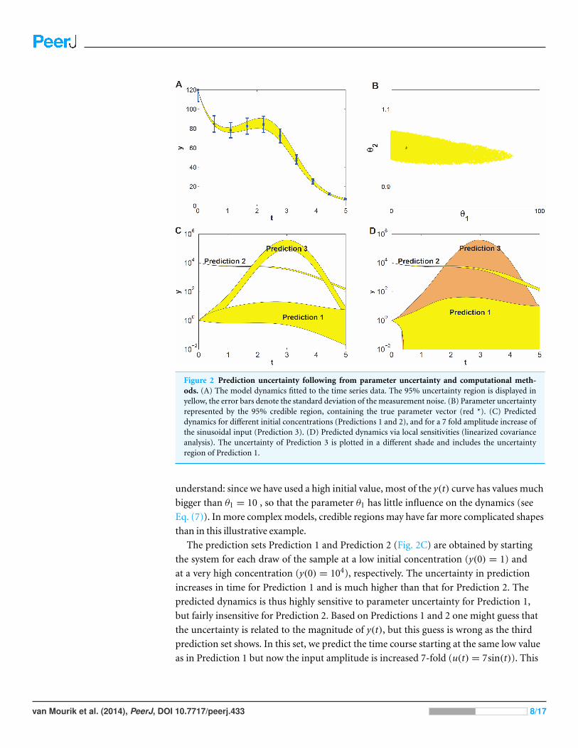
Figure 2 Prediction uncertainty following from parameter uncertainty and computational meth-ods. (A) The model dynamics fitted to the time series data. The 95% uncertainty region is displayed inyellow, the error bars denote the standard deviation of the measurement noise. (B) Parameter uncertaintyrepresented by the 95% credible region, containing the true parameter vector (red *). (C) Predicteddynamics for different initial concentrations (Predictions 1 and 2), and for a 7 fold amplitude increase ofthe sinusoidal input (Prediction 3). (D) Predicted dynamics via local sensitivities (linearized covarianceanalysis). The uncertainty of Prediction 3 is plotted in a different shade and includes the uncertaintyregion of Prediction 1.

understand: since we have used a high initial value, most of the y(t) curve has values much

bigger than θ1 = 10 , so that the parameter θ1 has little influence on the dynamics (see

Eq. (7)). In more complex models, credible regions may have far more complicated shapes

than in this illustrative example.

The prediction sets Prediction 1 and Prediction 2 (Fig. 2C) are obtained by starting

the system for each draw of the sample at a low initial concentration (y(0) = 1) and

at a very high concentration (y(0) = 104), respectively. The uncertainty in prediction

increases in time for Prediction 1 and is much higher than that for Prediction 2. The

predicted dynamics is thus highly sensitive to parameter uncertainty for Prediction 1,

but fairly insensitive for Prediction 2. Based on Predictions 1 and 2 one might guess that

the uncertainty is related to the magnitude of y(t), but this guess is wrong as the third

prediction set shows. In this set, we predict the time course starting at the same low value

as in Prediction 1 but now the input amplitude is increased 7-fold (u(t) = 7sin(t)). This

van Mourik et al. (2014), PeerJ, DOI 10.7717/peerj.433 8/17

drives the concentration dynamics into an oscillating motion which can be predicted

rather precisely (Fig. 2C), since now the input u(t) dominates the dynamics.

We also estimated prediction uncertainty via a local sensitivity analysis, namely

linearized covariance analysis (LCA, see the Supplemental Information for details). LCA

extrapolates parameter- and prediction uncertainty from a second- and first order Taylor

expansion, respectively, and does not take into account the higher order terms that in

this case constrain the credible region and the predictions, but note that linearization can

also lead to predictions that appear more precise than they really are. Consequently, LCA

dramatically overestimates the uncertainties of Predictions 1 and 3 (Fig. 2D).

This simple example illustrates that prediction uncertainty depends on the type of

prediction and is hard to foresee intuitively. We cannot evaluate the prediction uncertainty

on the basis of some simple guidelines after only inspecting the credible region of the

parameters. Because of the nonlinearities in the system, the credible region is untruthful

for evaluating predictions and their uncertainty (Savage, 2012). These results suggest that a

full computational uncertainty analysis, as performed here (Fig. 2C), has always to be done

in order to estimate the consequences of parameter uncertainty for prediction uncertainty.

The key element in this analysis is the sample representing the probability distribution of

the parameters.

It is convenient to quantify prediction uncertainty, that is, the variability among

predicted time courses. We do so on the basis of the quantity Q defined in Eq. (7) in the

Methods section, which expresses the deviation between two time courses, one being

calculated for an arbitrary set of parameter values and the other using the penalized

maximum likelihood estimator of the parameters. In our simulation studies, the latter

is replaced by the true parameter values. The quantity Q is calculated for each draw of the

parameters. The higher the Q value of a prediction, the higher its prediction uncertainty is.

Each prediction set yields 1000 values of Q, which are summarized by their 95% percentile,

indicated by Q0.95. Q0.95 values smaller than 1 indicate tight predictions. For example, the

Q0.95 values for Predictions 1, 2 and 3 in Fig. 2C are 18, 0.02 and 1.5, respectively. Even for

this simple model the uncertainty among different predictions thus varies by a factor 900

which is an order of 2.9 on logarithmic scale.

Scanning a variety of systems biology modelsNext, we study prediction uncertainty for six models from the BioModels database (Li et

al., 2010). We selected these models to represent some cross section of systems biology

models; The systems they represent greatly differ in numbers of variables, parameters, and

the types of equations. The parameters in these models represent process rates. The models

include circadian rhythm, metabolism, and signalling (Laub & Loomis, 1998; Levchenko,

Bruck & Sternberg, 2000; Tyson, 1991; Goldbeter, 1991; Vilar et al., 2002; Leloup & Goldbeter,

1999), see the Supplemental Information for details. For each model, a data set is created

in the same manner as described for the simple model above, with parameter values and

initial conditions as provided in the database. Each data set was analyzed using an MCMC

sampling algorithm yielding a sample of 1000 draws representing the distribution of the

van Mourik et al. (2014), PeerJ, DOI 10.7717/peerj.433 9/17

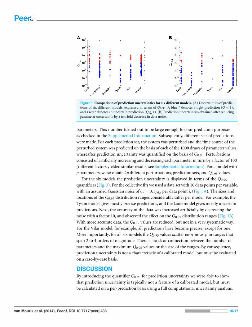
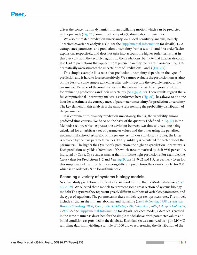
Figure 3 Comparison of prediction uncertainties for six different models. (A) Uncertainties of predic-tions of six different models, expressed in terms of Q0.95. A blue * denotes a tight prediction (Q < 1),and a red * denotes an uncertain prediction (Q ≥ 1). (B) Prediction uncertainties obtained after reducingparameter uncertainty by a ten-fold decrease in data noise.

parameters. This number turned out to be large enough for our prediction purposes

as checked in the Supplemental Information. Subsequently, different sets of predictions

were made. For each prediction set, the system was perturbed and the time course of the

perturbed system was predicted on the basis of each of the 1000 draws of parameter values,

whereafter prediction uncertainty was quantified on the basis of Q0.95. Perturbations

consisted of artificially increasing and decreasing each parameter in turn by a factor of 100

(different factors yielded similar results, see Supplemental Information). For a model with

p parameters, we so obtain 2p different perturbations, prediction sets, and Q0.95 values.

For the six models the prediction uncertainty is displayed in terms of the Q0.95

quantifiers (Fig. 3). For the collective fits we used a data set with 10 data points per variable,

with an assumed Gaussian noise of σi = 0.1yd,i per data point i. (Fig. 3A). The sizes and

locations of the Q0.95 distribution ranges considerably differ per model. For example, the

Tyson model gives mostly precise predictions, and the Laub model gives mostly uncertain

predictions. Next, the accuracy of the data was increased artificially by decreasing the

noise with a factor 10, and observed the effect on the Q0.95 distribution ranges (Fig. 3B).

With more accurate data, the Q0.95 values are reduced, but not in a very systematic way.

For the Vilar model, for example, all predictions have become precise, except for one.

More importantly, for all six models the Q0.95 values scatter enormously, in ranges that

span 2 to 4 orders of magnitude. There is no clear connection between the number of

parameters and the maximum Q0.95 values or the size of the ranges. By consequence,

prediction uncertainty is not a characteristic of a calibrated model, but must be evaluated

on a case-by-case basis.

DISCUSSIONBy introducing the quantifier Q0.95 for prediction uncertainty we were able to show

that prediction uncertainty is typically not a feature of a calibrated model, but must

be calculated on a per-prediction basis using a full computational uncertainty analysis.

van Mourik et al. (2014), PeerJ, DOI 10.7717/peerj.433 10/17

The adjective full stresses that the analysis must use (a representative sample of) the

distribution of the parameters and not only the 95% confidence region or credible

region of the parameters. The reason is that the parameter values inside the confidence

region may be outliers in terms of the prediction, just because of the nonlinearities of the

model (Savage, 2012). The key element is thus a faithful representation of the remaining

uncertainty in the parameters after fitting the model, in practical terms represented

by a sample of parameter values. This sample looks like a dataset with parameters as

columns and draws from the distribution as rows (Fig. 1). We used a sample of 1000

nearly independent draws obtained by thinning the MCMC chain. The sample is an

approximation of the full posterior distribution of the parameter values. The reliability

of this approximation is a point that deserves attention. We checked this by varying the

size of the sample and observing whether the results for the quantifier Q showed good

convergence. For the models studied in this paper, we found that this convergence was

indeed reached if we used a sample size of 1000 points, but for other cases it could happen

that this number must be larger.

The value of Q0.95 is interpretable. If Q0.95 ≥ 1, the uncertainty is so high that it

may obscure biological interpretation of a model prediction, whereas this is unlikely if

Q0.95 < 1. When the uncertainty indeed causes predictions to be biologically ambiguous,

Q0.95 could be incorporated as a design criterion in experimental design, i.e., additional

experiments can be designed or selected to minimize Q0.95 (Vanlier et al., 2012a; Vanlier et

al., 2012b; Apgar et al., 2010).

We adopted the Bayesian framework in our analysis. This framework has the advantage

that in the collective fits prior information on the parameters can be incorporated, such as

from general biological knowledge (Grandison & Morris, 2008) and previous experiments.

The prior in a Bayesian analysis is also a means to ensure that a parameter attains no

physically unrealistic values, when fitting the model to data. Current Bayesian MCMC

algorithms naturally lead to a sample of the posterior distribution that represents the

remaining uncertainty in the parameters. Alternatively, bootstrap sampling (Efron &

Tibshirani, 1993) could perhaps be used to create such a sample. MCMC can also be

applied to stochastic models. At each iteration the stochastic model has to be run again, so

that averaging/summarizing over the chain averages/integrates over the stochastic elements

in the model. As this simple approach often leads to very low MCMC acceptance rates,

it is advantageous to treat the stochastic elements as additional unknowns in the MCMC

with a Metropolis-within-Gibbs approach (ter Braak & Vrugt, 2008). Particle MCMC is a

promising method in this area in which proposals for the additional unknowns are made

via a particle filter (Andrieu, Doucet & Holenstein, 2010; Vrugt et al., 2013). Intersubject

variability is a simple form of a stochastic model in which only the parameters of the model

vary among subjects. The populations of models approach (Britton et al., 2013), which is

related to the Generalized Likelihood Uncertainty Estimation (GLUE) approach (Beven

& Binley, 1992) that is popular in hydrology, is a way to deal with such variability. The

formal Bayes approach (and thus MCMC) can also be used. Moreover, it can disentangle

van Mourik et al. (2014), PeerJ, DOI 10.7717/peerj.433 11/17

inter-subject variability (which cannot be reduced) and uncertainty (which can in

principle be reduced by collecting more data) as demonstrated for a pharmacokinetic

model in ter Braak & Vrugt (2008). A comparison of formal Bayes and GLUE can be found

in Vrugt et al. (2009).

Of course there are computational issues in the Bayesian approach which increase

with the number of the parameters and the complexity of the model. Gutenkunst et al.

(2007a) speeded up their Monte Carlo analysis (a random walk Metropolis algorithm) by

periodically updating the step size based on the current Fisher Information Matrix, but

such an updating scheme is generally not recommended as it may change the stationary

distribution of the chain (Roberts & Rosenthal, 2007). We used the adaptive MCMC

algorithm DE-MCz (ter Braak & Vrugt, 2008), that automatically adapts to the size and

shape of the posterior distribution. DE-MCz allows parallel computation when the chains

have access to a common store of past-sampled parameter values, and is designed to

quickly find and explore very elongated subspaces in the posterior distribution of the

parameters, which are due to sloppiness. Such subspaces point to problems with parameter

identifiability. An alternative approach to explore these problems is via profile likelihood

methods (Raue et al., 2009; Raue et al., 2010).

Systems biology models may be computationally expensive to evaluate, making

standard MCMC algorithms impractical as they require many evaluations. For our class

of dynamic computational models the likelihood of each sample is based on the time

integration of the model, which can be very demanding for large or stiff models. To confine

sampling and integration costs, model order reduction techniques may be of help to

speed up analysis (see Supplemental Information). However, the reduction errors affect

prediction uncertainty differs per model and per prediction.

An alternative approach is to locally approximate the likelihood function using param-

eter sensitivities. Applications in systems biology of the latter idea include a gene network

model in a Drosophila embryo (Ashyraliyev, Jaeger & Blom, 2008), a microbial growth

model (Schittkowski, 2007), and an in-silico gene regulatory network (Zak et al., 2003a).

This method is simple and has a very low computational demand since it avoids sampling,

but may lead to a highly erroneous estimation of prediction uncertainty (Gutenkunst et

al., 2007a), as we demonstrated (Fig. 2D). A better alternative is to use emulators and use

adaptive error modelling within the MCMC algorithm (Cui, Fox & O’Sullivan, 2011).

In this paper the analysis is carried out with noiseless data. The Hessian matrix

has full rank for each model, so all models are theoretically locally identifiable in the

neighbourhood of the penalized maximum likelihood parameter. However, in practice the

PML parameter might be hard to find or be non-unique due to noisy data. An alternative is

to define Q with respect to the average time course of the log-predictions (that is, averaging

across the sample of parameter values), as is mentioned in the end of the Methods section.

With noisy data, the uncertainty will increase compared to noiseless data, but the range of

uncertainties across different predictions, as expressed by quantifiers such as Q, is likely to

be similar to that in Fig. 3.

van Mourik et al. (2014), PeerJ, DOI 10.7717/peerj.433 12/17

For biologists it is not always essential to obtain quantitative predictions and a reviewer

asked about the uncertainty analysis of qualitative predictions. For this, the first step is

to convert any quantitative predicted time course into a qualitative prediction, such as

the statement that a certain metabolite or flux is going up, when a gene is over-expressed.

Once this step has been decided upon, the prediction for any particular set of parameter

values in the posterior sample is then either a simple yes (1) or no (0) or a value between 0

and 1 that measures the degree to which a single predicted time course corresponds with

the statement. The second step is then to determine the mean and variance of the values

obtained across the parameter sets in the posterior sample, which measure the extent to

which the model predicts what is stated, and the prediction uncertainty, respectively. Note

that for crisp (0/1) outcomes the mean is simply the fraction f of the parameter sets that

yields a yes, and the variance is f (1 − f ).

CONCLUSIONSOur survey of a variety of models shows that prediction uncertainty is hard to predict.

It turns out that it is practically impossible to establish the predictive power of a model

without a full computational uncertainty analysis of each individual prediction. In practice

this has strong consequences for the way models are transferred via the literature and

databases. We conclude that publication of a model in the open literature or a database

should not only involve the listing of the model equations, the parameter values with or

without confidence intervals or parameter sensitivities, but should also include a sample of,

say, 1000 draws representing the full (posterior) distribution of the parameters. Only

then prospective users are able to reliably perform a full computational uncertainty

analysis if they intend to use the model for prediction purposes. To this end, a software

package is made available online, including an exemplary parameter sample. In addition

we encourage to include experimental conditions, model assumptions, and used prior

knowledge in order to make the sample reproducible. This will decrease the chances of

error propagation, for example due to programming errors.

ACKNOWLEDGEMENTSThe authors would like to thank the reviewers for their comments and W Kruijer, H van

der Voet, S Schnabel, and E Boer for useful discussions.

ADDITIONAL INFORMATION AND DECLARATIONS

FundingThis work was supported by the Netherlands Consortium for Systems Biology (NCSB)

which is part of the Netherlands Genomics Initiative/Netherlands Organisation for

Scientific Research. The funders had no role in study design, data collection and analysis,

decision to publish, or preparation of the manuscript.

van Mourik et al. (2014), PeerJ, DOI 10.7717/peerj.433 13/17

Grant DisclosuresThe following grant information was disclosed by the authors:

The Netherlands Consortium for Systems Biology (NCSB).

Competing InterestsCajo ter Braak is an Academic Editor for PeerJ. Simon van Mourik and Jaap Molenaar are

co-financed by the Netherlands Consortium for Systems Biology.

Author Contributions• Simon van Mourik contributed reagents/materials/analysis tools, wrote the paper,

prepared figures and/or tables, reviewed drafts of the paper, software and literature

study.

• Cajo ter Braak contributed reagents/materials/analysis tools, wrote the paper, reviewed

drafts of the paper, software and literature study.

• Hans Stigter and Jaap Molenaar contributed reagents/materials/analysis tools, wrote the

paper, reviewed drafts of the paper, literature study.

Supplemental InformationSupplemental information for this article can be found online at http://dx.doi.org/

10.7717/peerj.433.

REFERENCESAlon U. 2006. An introduction to systems biology. Design principles of biological circuits. Boca Raton,

Florida: Chapman & Hall/CRC, 1–320.

Andrieu C, Doucet A, Holenstein R. 2010. Particle Markov chain Monte Carlo methods.Journal of the Royal Statistical Society: Series B (Statistical Methodology) 72(3):269–342DOI 10.1111/j.1467-9868.2009.00736.x.

Apgar JF, Witmer DK, White FM, Tidor B. 2010. Sloppy models, parameter uncertainty, and therole of experimental design. Molecular BioSystems 6(10):1890–1900 DOI 10.1039/b918098b.

Ashyraliyev M, Jaeger J, Blom JG. 2008. Parameter estimation and determinability analysis ap-plied to Drosophila gap gene circuits. BMC Systems Biology 2:83 DOI 10.1186/1752-0509-2-83.

Beck MB. 1987. Water quality modeling: a review of the analysis of uncertainty. Water ResourcesResearch 23(8):1393–1442 DOI 10.1029/WR023i008p01393.

Beven K, Binley A. 1992. The future of distributed models: model calibration and uncertaintyprediction. Hydrological Processes 6(3):279–298 DOI 10.1002/hyp.3360060305.

Britton OJ, Bueno-Orovio A, Van Ammel K, Lu HR, Towart R, Gallacher DJ, Rodriguez B. 2013.Experimentally calibrated population of models predicts and explains intersubject variability incardiac cellular electrophysiology. Proceedings of the National Academy of Sciences of the UnitedStates 110(23):E2098–E2105 DOI 10.1073/pnas.1304382110.

Brown KS, Hill CC, Calero GA, Myers CR, Lee KH, Sethna JP, Cerione RA. 2004. The statisticalmechanics of complex signaling networks: nerve growth factor signaling. Physical Biology1(3):184–195 DOI 10.1088/1478-3967/1/3/006.

Brown KS, Sethna JP. 2003. Statistical mechanical approaches to models with many poorly knownparameters. Physical Review E 68(2):1–9 DOI 10.1103/PhysRevE.68.021904.

van Mourik et al. (2014), PeerJ, DOI 10.7717/peerj.433 14/17

Buchler NE, Louis M. 2008. Molecular titration and ultrasensitivity in regulatory networks.Journal of Molecular Biology 384(5):1106–1119 DOI 10.1016/j.jmb.2008.09.079.

Cui T, Fox C, O’Sullivan MJ. 2011. Bayesian calibration of a large-scale geothermal reservoirmodel by a new adaptive delayed acceptance Metropolis Hastings algorithm. Water ResourcesResearch 47(10) DOI 10.1029/2010WR010352.

Efron B, Tibshirani R. 1993. An introduction to the bootstrap. Vol. 57. Boca Raton, Florida:Chapman & Hall/CRC, 1–456.

Goldbeter A. 1991. A minimal cascade model for the mitotic oscillator involving cyclin and cdc2kinase. Proceedings of the National Academy of Sciences of the United States 88(20):9107–9111DOI 10.1073/pnas.88.20.9107.

Grandison S, Morris RJ. 2008. Biological pathway kinetic rate constants are scale-invariant.Bioinformatics 24(6):741–743 DOI 10.1093/bioinformatics/btn041.

Gutenkunst RN, Casey FP, Waterfall JJ, Myers CR, Sethna JP. 2007a. Extracting falsifiablepredictions from sloppy models. Annals of the New York Academy of Sciences 1115(1):203–211DOI 10.1196/annals.1407.003.

Gutenkunst RN, Waterfall JJ, Casey FP, Brown KS, Myers CR, Sethna JP. 2007b. Universallysloppy parameter sensitivities in systems biology models. PLoS Computational Biology3(10):e189 DOI 10.1371/journal.pcbi.0030189.

Hawkins E, Sutton R. 2009. The potential to narrow uncertainty in regional climate predictions.Bulletin of the American Meteorological Society 90(8):1095–1107DOI 10.1175/2009BAMS2607.1.

Jaynes ET. 2003. Probability theory: the logic of science. Vol. 1. Cambridge: Cambridge UniversityPress, 1–727.

Klipp E, Herwig R, Kowald A, Wierling C, Lehrach H. 2008. Systems biology in practice: concepts,implementation and application. Vol. 1. Weinheim: John Wiley & Sons, 486.

Kreutz C, Raue A, Kaschek D, Timmer J. 2013. Profile likelihood in systems biology. FEBS Journal280(11):2564–2571 DOI 10.1111/febs.12276.

Laub MT, Loomis WF. 1998. A molecular network that produces spontaneous oscillations inexcitable cells of Dictyostelium. Molecular Biology of the Cell 9(12):3521–3532DOI 10.1091/mbc.9.12.3521.

Leloup JC, Goldbeter A. 1999. Chaos and birhythmicity in a model for circadian oscillations ofthe PER and TIM proteins in Drosophila. Journal of Theoretical Biology 198(3):445–459DOI 10.1006/jtbi.1999.0924.

Levchenko A, Bruck J, Sternberg PW. 2000. Scaffold proteins may biphasically affect the levels ofmitogen-activated protein kinase signaling and reduce its threshold properties. Proceedings ofthe National Academy of Sciences of the United States 97(11):5818–5823DOI 10.1073/pnas.97.11.5818.

Li C, Donizelli M, Rodriguez N, Dharuri H, Endler L, Chelliah V, Li L, He E, Henry A,Stefan MI, Snoep JL, Hucka M, Le Novere N, Laibe C. 2010. Biomodels database: an enhanced,curated and annotated resource for published quantitative kinetic models. BMC Systems Biology4(1):92 DOI 10.1186/1752-0509-4-92.

MacKay DJC. 2003. Information theory, inference and learning algorithms. Vol. 1. Cambridge:Cambridge University Press, 1–628.

Maerkl SJ, Quake SR. 2007. A systems approach to measuring the binding energy landscapes oftranscription factors. Science 315:233–237 DOI 10.1126/science.1131007.

van Mourik et al. (2014), PeerJ, DOI 10.7717/peerj.433 15/17

Omlin M, Reichert P. 1999. A comparison of techniques for the estimation of model predictionuncertainty. Ecological Modelling 115(1):45–59 DOI 10.1016/S0304-3800(98)00174-4.

Raue A, Becker V, Klingmuller U, Timmer J. 2010. Identifiability and observability analysis forexperimental design in nonlinear dynamical models. Chaos 20(4):1–8 DOI 10.1063/1.3528102.

Raue A, Kreutz C, Maiwald T, Bachmann J, Schilling M, Klingmuller U, Timmer J. 2009.Structural and practical identifiability analysis of partially observed dynamical models byexploiting the profile likelihood. Bioinformatics 25(15):1923–1929DOI 10.1093/bioinformatics/btp358.

Raue A, Kreutz C, Theis FJ, Timmer J. 2013. Joining forces of Bayesian and frequentistmethodology: a study for inference in the presence of non-identifiability. PhilosophicalTransactions of the Royal Society A: Mathematical, Physical and Engineering Sciences371(1984):1–10.

Robert CP, Marin J, Rousseau J. 2011. Bayesian inference and computation. In: Stumpf MPH,Balding DJ, Girolami M, eds. Handbook of statistical systems biology. West Sussex: John Wiley &Sons, Ltd., 39–65

Roberts GO, Rosenthal JS. 2007. Coupling and ergodicity of adaptive Markov chain Monte Carloalgorithms. Journal of Applied Probability 44(2):458–475 DOI 10.1239/jap/1183667414.

Savage SL. 2012. The flaw of averages: why we underestimate risk in the face of uncertainty.Hoboken, New Jersey: Wiley, 1–288.

Schittkowski K. 2007. Experimental design tools for ordinary and algebraic differential equations.Industrial & Engineering Chemistry Research 46(26):9137–9147 DOI 10.1021/ie0703742.

Stumpf MPH, Balding DJ, Girolami M. 2011. Handbook of statistical systems biology. West Sussex:Wiley Online Library, 1–530.

ter Braak CJF, Vrugt JA. 2008. Differential Evolution Markov Chain with snooker updater andfewer chains. Statistics and Computing 18:435–446 DOI 10.1007/s11222-008-9104-9.

Teusink B, Passarge J, Reijenga CA, Esgalhado E, van der Weijden CC, Schepper M, Walsh MC,Bakker BM, van Dam K, Westerhoff HV, Snoep JL. 2000. Can yeast glycolysis be understood interms of in vitro kinetics of the constituent enzymes? Testing biochemistry. European Journal ofBiochemistry 267(17):5313–5329 DOI 10.1046/j.1432-1327.2000.01527.x.

Tyson JJ. 1991. Modeling the cell division cycle: cdc2 and cyclin interactions. Proceedings of the Na-tional Academy of Sciences of the United States 88(16):7328–7332 DOI 10.1073/pnas.88.16.7328.

van Mourik S, van Dijk AD, deGee M, Immink RG, Kaufmann K, Angenent GC, van Ham RC,Molenaar J. 2010. Continuous-time modeling of cell fate determination in Arabidopsis flowers.BMC Systems Biology 4(1):101 DOI 10.1186/1752-0509-4-101.

Vanlier J, Tiemann CA, Hilbers PAJ, van Riel NAW. 2012a. An integrated strategy for predictionuncertainty analysis. Bioinformatics 28(8):1130–1135 DOI 10.1093/bioinformatics/bts088.

Vanlier J, Tiemann CA, Hilbers PAJ, van Riel NAW. 2012b. A Bayesian approach to targetedexperiment design. Bioinformatics 28(8):1136–1142 DOI 10.1093/bioinformatics/bts092.

Vilar JM, Kueh HY, Barkai N, Leibler S. 2002. Mechanisms of noise-resistance in geneticoscillators. Proceedings of the National Academy of Sciences of the United States 99(9):5988–5992DOI 10.1073/pnas.092133899.

Vrugt JA, ter Braak CJ, Diks CG, Schoups G. 2013. Hydrologic data assimilation using particleMarkov chain Monte Carlo simulation: theory, concepts and applications. Advances in WaterResources 51:457–478 DOI 10.1016/j.advwatres.2012.04.002.

van Mourik et al. (2014), PeerJ, DOI 10.7717/peerj.433 16/17

Vrugt JA, Ter Braak CJ, Gupta HV, Robinson BA. 2009. Equifinality of formal (DREAM) andinformal (GLUE) Bayesian approaches in hydrologic modeling? Stochastic EnvironmentalResearch and Risk Assessment 23(7):1011–1026 DOI 10.1007/s00477-008-0274-y.

Zak DE, Gonye GE, Schwaber JS, Doyle FJ. 2003a. Importance of input perturbations andstochastic gene expression in the reverse engineering of genetic regulatory networks: insightsfrom an identifiability analysis of an in silico network. Genome Research 13(11):2396–2405DOI 10.1101/gr.1198103.

Zak DE, Pearson RK, Vadigepalli R, Gonye GE, Schwaber JS, Doyle Iii FJ. 2003b.Continuous-time identification of gene expression models. OMICS: A Journal of IntegrativeBiology 7(4):373–386 DOI 10.1089/153623103322637689.

van Mourik et al. (2014), PeerJ, DOI 10.7717/peerj.433 17/17